Embed Size (px)
Citation preview

TR-EE 89-49
August 1989
MODELING, SIMULATION, ANDANALYSIS OF OPTICAL REMOTE
SENSING SYSTEMS
J. P. Kerekes
D. A. Landgrebe
School of Electrical Engineering
Purdue University
West Lafayette, Indiana 47907
This research was supported in part by the National ScienceFoundation under Grant ECS 8507405 and National Aeronautics and
Space Administration Grant NAGW-925.
https://ntrs.nasa.gov/search.jsp?R=19900017060 2018-07-08T16:18:53+00:00Z


ii
TABLE OF CONTENTS
Page
LIST OF TABLES ............................................................................................................. iv
LIST OF FIGURES ........................................................................................................... vi
LIST OF NOTATIONS .................................................................................................... xii
ABSTRACT .................................................................................................................... xvii
CHAPTER 1 - INTRODUCTION .................................................................................... 1
1.1 Background and Objective of the Investigation ..................................... 11.2 Remote Sensing System Description ..................................................... 21.3 Related Work ............................................................................................... 8
1.4 Report Organization ................................................................................. 10
CHAPTER 2 - REMOTE SENSING SYSTEM MODELING ANDSIMULATION ......................................................................................... 11
2.1 Overview of System Model ..................................................................... 112.2 Scene Models ........................................................................................... 13
2.2.1 Surface Reflectance Modeling ..................................................... 142.2.2 Solar and Atmospheric Modeling ................................................ 25
2.3 Sensor Modeling ...................................................................................... 472.3.1 Sampling Effects ............................................................................. 482.3.2 Electrical Noise Modeling ............................................................. 522.3.3 HIRIS Model ..................................................................................... 542.3.4 Radiometric Performance Measures ........................................... 61
2.4 Processing ................................................................................................. 632.4.1 Radiometric Processing ................................................................. 652.4.2 Geometric Processing .................................................................... 652.4.3 Data Reduction ................................................................................ 66
2.4.4 Class Separability Measures ....................................................... 672.4.5 Classification Algorithms ............................................................... 68
2.5 Summary and Discussion ....................................................................... 69


iii
Page
CHAPTER 3- ANALYTICAL SYSTEM MODEL ....................................................... 71
3.1 Model Overview ........................................................................................ 71
3.2 Analytical Expressions ............................................................................. 733.2.1 Reflectance Statistics ..................................................................... 73
3.2.2 Atmospheric Effects ........................................................................ 743.2.3 Spatial Effects .................................................................................. 753.2.4 Spectral Effects ............................................................................... 773.2.5 Noise Model ..................................................................................... 783.2.6 Feature Selection ........................................................................... 793.2.7 Error Estimation ............................................................................... 79
3.3 Comparison Between the Analytical and Simulation Models .......... 80
CHAPTER 4 - APPLICATION TO IMAGING SPECTROMETER SYSTEMANALYSIS .............................................................................................. 83
4.1 Introduction ................................................................................................ 834.2 Radiometric Performance ........................................................................ 84
4.3 Comparison of Simulation and Analytic Model Performance .......... 994.4 System Parameter Studies ................................................................... 1074.5 Interrelated Parameter Effects .............................................................. 123
4.6 Feature Selection Experiments ............................................................ 1344.7 Summary and Conclusions .................................................................. 140
CHAPTER 5 - CONCLUSIONS AND SUGGESTIONS FOR FUTHER WORK.143
LIST OF REFERENCES ............................................................................................. 147
APPENDICES
Appendix A
Appendix BAppendix CAppendix DAppendix E
Expected Variance of a Two DimensionalAutoregressive Process ....................................................... 155Interpolation Algorithm ......................................................... 160LOWTRAN 7 Input File ......................................................... 162Sensor Descriptions ............................................................. 167Analytical System Model Program Listing ....................... 173

iv
Table
1.1
2.1
2.2
2.3
2.4
2.5
2.6
2.7
2.8
2.9
2.10
2.11
2.12
2.13
2.14
2.15
2.16
2.17
LIST OF TABLES
Page
Simulation Studies .............................................................................................. 9
Typical Spatial Model Parameters ................................................................. 20
Spatial Correlation Coefficients for Hand County, South Dakota ............ 21
Sequence in Generating a Simulated Surface Reflectance Array ........... 24
Example LOW'IRAN 7 Parameters ................................................................. 31
Diffuse Irradiance Constant Values ................................................................ 34
Default Values of Atmospheric Parameters .................................................. 35
Data Set for Hand County, South Dakota, July 26, 1978 ........................... 42
Description of Test Fields ................................................................................. 43
Conversion Constants Between Radiance and Digital Counts ................ 43
Scene Conditions at Time of Observations .................................................. 44
LOWTRAN Settings for Experiment ................................................................ 44
Atmospheric Components for the Hand County Test Site ......................... 45
Comparison of Actual and Simulated Radiances (in mW/(cm2-sr)) forTest Site in Hand County, SD ......................................................................... 45
Sources and Types of Radiometric Errors .................................................... 53
HIRIS Functional Parameters .......................................................................... 54
Parameters of Detector Arrays in Terms of Electrons (e) .......................... 59
Example Processing Functions ....................................................................... 64

V
Table
2.18
3.1
4.1
4.2
4.3
4.4
4.5
4.6
4.7
4.8
4.9
4.10
4.11
4.12
4.13
4.14
Page
Summary of System Parameters Implemented in Simulation .................. 70
System Factors Not Included In Analytical Model ....................................... 80
Kansas Winter Wheat Data Set ....................................................................... 84
Radiometdc Study Baseline System Configuration .................................... 85
Radiometric Performance Parameters Studied and Their Variations ...... 88
System Configuration for Comparison Test ................................................ 100
Optimal Feature Set for Kansas Winter Wheat Data Set .......................... 102
Classification Accuracy of Base System Configuration ............................ 102
Increments Used in Ground Size Experiment ............................................ 104
Classification Accuracies of Gaussian vs. Measured PSF ...................... 106
System Configuration for Parameter Studies ............................................. 108
Parameters and Their Variation in Section 4.4 .......................................... 108
Summary Results for System Parameter Experiments ............................. 121
Parameter Interrelationship Studies ............................................................ 123
Wavelength Bands Combined fQr the Various Feature Sets ................... 134
Classes and Fields Used to Compute Statistics for the Spring WheatTest Scene ........................................................................................................ 138
AppendixTable
D.1
D.2
D.3
D.4
D.5
D.6
MMS General Parameters ............................................................................. 167
MMS Band and Noise Parameters ............................................................... 167
MSS General Parameters .............................................................................. 169
MSS Band and Noise Parameters ............................................................... 169
TM General Parameters ................................................................................. 171
TM Band and Noise Parameters ................................................................... 171

vi
LIST OF FIGURES
Figure
1.1
1.2
1.3
2.1
2.2
2.3
2.4
2.5
2.6
2.7
2.8
2.9
2.10
2.11
2.12
2.13
2.14
Page
Remote Sensing System Pictorial Description .............................................. 3
Noise Sources ...................................................................................................... 6
Signal Sources .................................................................................................... 7
Remote Sensing System Model ..................................................................... 12
Scene Model Block Diagram ........................................................................... 13
Scene Geometry ................................................................................................ 15
Correlation Coefficients of Winter Wheat Field ............................................ 22
Atmospheric Effects on Spectral Radiance Received by Sensor ............. 27
Optical Thickness '_ vs. Visibility ...................................................................... 30
Optical Thickness vs. Wavelength .................................................................. 30
Ratio of Direct Irradiance to Total Irradiance vs. Total Optical PathLength .................................................................................................................. 33
Effect of Meteorological Range on Direct Solar Spectral Irradiance ....... 36
Effect of Solar Zenith Angle on Direct Solar Spectral Irradiance ............. 36
Effect of Meteorological Range on Total Solar Spectral Irradiance ......... 37
Effect of Solar Zenith Angle on Total Solar Spectral Irradiance ............... 37
Effect of Meteorological Range on Diffuse Solar Spectral Irradiance ..... 38
Effect of Solar Zenith Angle on Diffuse Solar Spectral Irradiance ........... 38

vii
Figure
2.15
2.16
2.17
2.18
2.19
2.20
2.21
2.22
2.23
2.24
2.25
2.26
2.27
2.28
3.1
4.1
4.2
4.3
4.4
4.5
4.6
4.7
4.8
Page
Effect of Meteorological Range on Spectral Transmittance ....................... 39
Effect of Sensor Zenith Angle on Spectral Transmittance ......................... 39
Effect of Meteorological Range on Path Spectral Radiance ...................... 40
Effect of Solar Zenith Angle on Path Spectral Radiance ............................ 40
Effect of Sensor Zenith Angle on Path Spectral Radiance ........................ 41
Effect of Surface Albedo on Path Spectral Radiance ................................. 41
Plot of Landsat vs. Simulated Radiances ...................................................... 46
Sensor System Components .......................................................................... 47
Noise Model of Sensor ..................................................................................... 52
HIRIS Model Block Diagram ............................................................................ 55
Spectral Transmittance of Optics .................................................................... 56
Normalized Spatial Response ........................................................................ 57
Spectral Quantum Efficiency ........................................................................... 58
Shot Noise vs. Signal Level ............................................................................ 60
Analytical System Model Block Diagram ...................................................... 71
Mean and Variation of the Surface Reflectance of the Kansas WinterWheat Data Set of Table 4.1 ............................................................................ 85
Mean and Variation of Image Vector as Received by HIRIS ..................... 86
Voltage and Power SNR for Typical Reflectance ........................................ 87
NEAp for Typical Reflectance .......................................................................... 87
SNR for Varying Meteorological Ranges ...................................................... 89
NEAp for Varying Meteorological Ranges .................................................... 89
SNR for Varying Solar Angles ......................................................................... 90
NEZ_o for Varying Solar Angles ....................................................................... 90

viii
Figure
4.9
4.10
4.11
4.12
4.13
4.14
4.15
4.16
4.17
4.18
4.19
4.20
4.21
4.22
4.23
4.24
4.25
4.26
4.27
4.28
4.29
4.30
Page
SNR for Varying View Angles .......................................................................... 91
NEAp for Varying View Angles ........................................................................ 91
SNR for Various Surface Albedoes ................................................................ 92
NEAp for Various Albedoes ............................................................................. 92
SNR for Varying Factors of Shot Noise ......................................................... 93
NEAp for Varying Factors of Shot Noise ....................................................... 93
SNR for Varying Factors of Read Noise ........................................................ 94
NEAp for Varying Factors of Read Noise ...................................................... 94
SNR for Varying Radiometric Resolution ...................................................... 95
NEAp for Various Radiometric Resolutions .................................................. 95
SNR for Various IMC Gain Settings ............................................................... 96
NEAp for Various IMC Gain Settings ............................................................. 96
SNR for Various Levels of Relative Calibration Error ................................. 97
NEAp for Various Levels of Relative Calibration Error ............................... 97
Simulated Image of Comparison Test Scene at Z=1.70 I_m .................... 101
Classification Accuracy vs. Scene Spatial Correlation Coefficient ........ 103
Classification Accuracy vs. Ground Size of Scene Cells ......................... 104
Classification Accuracy vs. Sensor View Angle ......................................... 105
Classification Accuracy vs. Number of Training Samples ....................... 107
Effect of Spatial Correlation (p=px=Py) on SNR ......................................... 109
Effect of Spatial Correlation (p=px=Py) on Classification Accuracy ........ 109
Effect of Meteorological Range on SNR ...................................................... 110

ix
Figure
4.31
4.32
4.33
4.34
4.35
4.36
4.37
4.38
4.39
4.40
4.41
4.42
4.43
4.44
4.45
4.46
4.47
4.48
4.49
4.50
4.51
4.52
4.53
Page
Effect of Meteorological Range on Classification Accuracy ..................... 110
Effect of Solar Zenith Angle on SNR ............................................................ 111
Effect of Solar Zenith Angle on Classification Accuracy ........................... 111
Effect of Sensor Zenith Angle on SNR ......................................................... 112
Effect of Sensor Zenith Angle on Classification Accuracy ....................... 112
Effect of Number of Scene Cells Within Sensor IFOV on SNR ............... 113
Effect of Number of Scene Cells Within Sensor IFOV on Classification
Accu racy ............................................................................................................ 113
Effect of Shot Noise (Nominal = 1.0) on SNR ............................................. 114
Effect of Shot Noise (Nominal = 1.0) on Classification Accuracy ........... 11 4
Effect of Read Noise (Nominal = 1.0) on SNR ............................................ 11 5
Effect of Read Noise (Nominal = 1.0) on Classification Accuracy .......... 115
Effect of IMC Gain State on SNR .................................................................. 116
Effect of IMC Gain State on Classification Accuracy ................................. 116
Effect of Radiometric Resolution on SNR .................................................... 11 7
Effect of Radiometric Resolution on Classification Accuracy ................... 11 7
Effect of Relative Calibration Error on SNR ................................................ 118
Effect of Relative Calibration Error on Classification Accuracy ............... 118
Effect of Absolute Radiometric Error on SNR ............................................. 119
Effect of Absolute Radiometric Error on Classification Accuracy ............ 119
Effect of Number of Processing Features on SNR ..................................... 120
Effect of Number of Processing Features on Classification Accuracy ...120
Accuracy vs. Voltage SNR for System Parameter Experiments ............. 122
Accuracy vs. Power SNR for System Parameter Experiments ................ 122

Figure
4.54
4.55
4.56
4.57
4.58
4.59
4.60
4.61
4.62
4.63
4.64
4.65
4.66
4.67
4.68
4.69
4.70
4.71
4.72
4.73
4.74
4.75
Page
Effect of MeteorologicalRangeand View Angle for esolar=0°..................124
Effect of Meteorological Rangeand View Angle for esolar=30° ...............124
Effect of MeteorologicalRangeand View Angle for esoJar=60° ...............125
Effect of IFOV Size (in Scene Cells) and Spatial CorrelationCoefficient .........................................................................................................125
Effect of Meteorological Rangeand Shot Noise........................................126
Effect of Meteorological Rangeand Read Noise.......................................126
Effect of MeteorologicalRangeand IMC.....................................................127
Effectof MeteorologicalRangeon RadiometricResolution.....................127
Effect of Meteorological Rangeand Various Noise Sources Alone.......128
Effect of Solar Angle and Shot Noise..........................................................128
Effect of View Angle and Shot Noise...........................................................129
Effect Solar Angle and IMC Gain State.......................................................129
Effect of View Angle and IMC Gain State....................................................130
Effect of MeteorologicalRange and Number of Features........................130
Effectof Solar Angleand Numberof Features...........................................131
Effect of Atmosphere With/WithoutNoise for Path RadianceModelWith No Surface Reflectance Dependence................................................133
Voltage and Power SNR for the Various FeatureSets of Table 4.13....135
Classification Accuracy for the Various FeatureSets of Table 4.13 ......135
Feature Set Performancevs. MeteorologicalRange................................136
Feature Set Performancevs. Solar Angle..................................................137
Feature Set Performancevs. View Angle ...................................................137
SNRfor Various FeatureSetsand SWVarietyScene.............................139

xi
Figure Page
4.76 Classification Accuracy for Various Feature Sets and SW VarietyScene.................................................................................................................139
AppendixFigure
A.1
D.1
D.2
D.3
D.4
D.5
D.6
Quarter-Plane ImageAR Model....................................................................156
MMS Spectral Responsefor Bands 1 through 5 .......................................168
MMS Spectral Responsefor Bands 6 through 10.....................................168
MSS SpectralResponse................................................................................170
MSS Spatial Response..................................................................................170
TM Spectral Response...................................................................................172
TM SpatialResponse......................................................................................172

xii
LIST OF NOTATIONS
Symbols used for the various variables and parameters are defined
below, along with the units where appropriate.
Symbol
Ax
Ay
amn,bmn
B
Bkl
B(_,)
B+(_)
Ci
D
d(i,j,I)
ER
EL, Diffuse
E_Direct
Explanation (units)
Sum of hx(o) coefficients
Sum of hy(o) coefficients
Spatial model parameters for wavelengths m and n
Sensor spectral response matrix used in analytical model
Bhattacharyya distance between classes k and I
Conversion factor relating the incident spectral radiance to thesignal level in the sensor detectors
Product of the spectral radiance from a completely reflectingsurface and the conversion to the signal level in the detectors
AR model spatial parameters
Fractal dimension
Image level at pixel (i,j) for sensor band I
Absolute radiometric error level
Diffuse solar spectral irradiance incident on Earth's surface
(mW/cm2-_m)
Direct solar spectral irradiance incident on Earth's surface
(mW/cm2-p.m)

,.o
XIII
E_.,Exo
E;L,Total
F
F
Gx
Gy
gk(i,j)
gx
gy
H
h(u,v)
hx(')
hy(.)
JF
K
L
LFull,I
L_.,Scene(°)
L_sensor(x,y)
Lk,Path
1
L_.,Path
Exoatmospheric solar spectral irradiance incident on Earth's
surface (mW/cm2-11m)
Total (direct plus diffuse) solar spectral irradiance incident on
Earth's surface (mW/cm2-1im)
Band selection matrix for spectral compression
Full scale electron level in HIRIS model
Ground size of scene cell across scene (meters)
Ground size of scene cell down scene (meters)
Value of discriminant function for class k at pixel (i,j)
Ground size of PSF step across scene (meters)
Ground size of PSF step down scene (meters)
Altitude of sensor (meters)
2-dimensional point spread function of sensor
Across track line spread function
Down scene line spread function
Multiclass distance measure
Number of land cover classes in scene
Number of spectral bands in sensor
Full scale radiance for sensor band I (mW/cm2-sr)
Scene spectral radiance (mW/cm2-sr)
Spectral radiance incident on sensor from scene location (x,y)
(mW/cm2-1_m-sr)
Path spectral radiance incident on sensor (mW/cm2-1_m-sr)
Path spectral radiance with albedo = 1 (mW/cm2-1_m-sr)
xiv
o
L_.,Path
1-0
Lk.,Path
M
N(I)
nl(°), n2(')
0
P
Pk
Q
r(x,y)
ro.x, ro,y
S
S'
S"
Sb
SE
Sw
Sx
Sy
sl(m)
T_Atm
Path spectral radiance with albedo = 0 (mW/cm2-11m-sr)
Path spectral radiance difference for albedoes 0 and 1
(mW/cm2-pm-sr)
Dimension of high resolution spectral reflectance vectors
Spectral bandwidth normalizing factor for sensor band I
Zero mean, unit variance Gaussian random numbers
Number of coefficients in across scene spatial response
Number of coefficients in down scene spatial response
Estimate of classification accuracy
Apriori probability of class k
Number of radiometric bits of sensor
Surface scalar reflectance array
Radius of spatial response in analytical model
Received signal in detectors
Received signal plus dark current in detectors
Received signal plus noise and calibration error in detectors
L x L between class scatter matrix
L x L covariance matrix of image for class k
L x L within class scatter matrix
Across track ground sampling interval (meters)
Down scene ground sampling interval (meters)
Spectral response of sensor
Spectral transmissivity of atmosphere

XV
Ws
XA
Xk
2k
z(.)
P
A;L
AU
AV
AW
AZ
_solar
_view
Ak
Acal
Aquant
Aread
Atmospheric surface meteorological range (Kilometers)
Spatial weighting function in sensor model
Adjacent surface reflectance
Surface reflectance vector for class k
Mean image or feature vector for class k
Zero mean, unit variance Gaussian random numbers
Volume extinction coefficient (Km -1)
Spectral resolution of scene (l_m)
Angular distance between hx(o ) coefficients (radians)
Angular distance between hy(o) coefficients (radians)
Across track sampling interval (radians)
Down scene sampling interval (radians)
M x M eigenvector matrix of spectral reflectance covariancematrix for class k
Azimuthal angle of solar illumination (degrees)
Azimuthal angle of view (degrees)
M x M diagonal eigenvalue matrix of spectral reflectance
covariance matrix for class k
L x L diagonal matrix of relative calibration error variances
L x L diagonal matrix of quantization noise variances
L x L diagonal matrix of read noise variances

xvi
J_shot
J_kther m
Pk
P(x,y)
Px, Py
ZA
T--,k
Oc(I)
s(I)
O"u
'¢p,X,
_solar
Oview
L x L diagonal matrix of shot noise variances
L x L diagonal matrix of thermal noise variances
Wavelength (l_m)
M x 1 mean vector of spectral reflectance for class k
M x 1 vector of spectral reflectance of surface at location (x,y)
Spatial autocorrelation coefficients
Covariance matrix of average spectral reflectance
Covariance matrix of spectral reflectance or image features for
class k
Calibration error standard deviation for sensor band I
Shot noise standard deviation for sensor band I
Thermal noise standard deviation for sensor band I
Standard deviation of driving process for AR model
Spectral optical thickness of atmosphere
Spectral optical path length
Zenith angle of solar illumination (degrees)
Zenith viewing angle (degrees)

xvii
ABSTRACT
Kerekes, John Paul. Ph.D., Purdue University, August 1989. Modeling,Simulation, and Analysis of Optical Remote Sensing Systems. Major Professor:David A. Landgrebe.
Remote Sensing of the Earth's resources from space-based sensors has
evolved in the past twenty years from a scientific experiment to a commonly
used technological tool. The scientific applications and engineering aspects of
remote sensing systems have been studied extensively. However, most of
these studies have been aimed at understanding individual aspects of the
remote sensing process while relatively few have studied their interrelations.
A motivation for studying these interrelationships has arisen with the
advent of highly sophisticated configurable sensors as part of the Earth
Observin System (EOS) proposed by NASA for the 1990's. These instruments
represent a tremendous advance in sensor technology with data gathered in
nearly 200 spectral bands, and with the ability for scientists to specify many
observational parameters, tt will be increasingly necessary for users of remote
sensing systems to understand the tradeoffs and interrelationships of system
parameters.
In this report, two approaches to investigating remote sensing systems
are developed. In one approach, detailed models of the scene, the sensor, and
the processing aspects of the system are implemented in a discrete simulation.
This approach is useful in creating simulated images with desired
characteristics for use in sensor or processing algorithm development.


XVIII
A less complete, but computationally simpler method based on a
parametric model of the system is also developed. In this analytical model the
various informational classes are parameterized by their spectral mean vector
and covariance matrix. These class statistics are modified by models for the
atmosphere, the sensor, and processing algorithms and an estimate made of
the resulting classification accuracy among the informational classes.
Application of these models is made to the study of the proposed High
Resolution Imaging Spectrometer (HIRIS). The interrelationships among
observational conditions, sensor effects, and processing choices are
investigated with several interesting results.
Reduced classification accuracy in hazy atmospheres is seen to be due
not only to sensor noise, but also to the increased path radiance scattered from
the surface.
The effect of the atmosphere is also seen in its relationship to view angle.
In clear atmospheres, increasing the zenith view angle is seen to result in an
increase in classification accuracy due to the reduced scene variation as the
ground size of image pixels is increased. However, in hazy atmospheres the
reduced transmittance and increased path radiance counter this effect and
result in decreased accuracy with increasing view angle.
The relationship between the Signal-to-Noise Ratio (SNR) and
classification accuracy is seen to depend in a complex manner on spatial
parameters and feature selection. Higher SNR values are seen to not always
result in higher accuracies, and even in cases of low SNR feature sets chosen
appropriately can lead to high accuracies.

1 Chapter 1 - Introduction
CHAPTER 1
INTRODUCTION
1.1 Background and Objective of the Investigation
Remote sensing is defined (Swain and Davis, 1978) as "...the science of
deriving information about an object from measurements made at a distance
from the object, i.e., without actually coming in contact with it." In the context of
observing the Earth, the sensing instruments have evolved from cameras
tethered to balloons, aerial multispectral scanners, to satellite-borne imaging
arrays. Applications have been many, and remote sensing of the Earth for land
resource analysis has developed into a common and useful technological tool.
Countless projects have used remotely sensed data to assess crop
production (MacDonald and Hall, 1978), crop disease (MacDonald, et al.,
1972), urban growth (Jensen, 1981), and wetland acreage (Carter and
Schubert, 1974) as a few examples. The technology of remote sensing has
been studied extensively and is well documented in texts by Swain and Davis
(1978), Colwell (1983), Richards (1986), and Asrar (1989).
While the various aspects of the remote sensing process have been well
documented, the interrelationships among these process components have
been studied comparatively little, especially in regard to sources of error or
noise in the process. Landgrebe and Malaret (1986) looked at the effect of
sensor noise on classification error in one of the few studies of this type, but
there are many more parameters and effects that interrelate.
A motivation for studying these interrelationships has arisen with the
forthcoming deployment of configurable sensors. As part of the Earth Observing
System (EOS) program of the 1990's, several instruments will allow the

Chapter 1 - Introduction 2
capability for a scientist to specify the observational conditions under which
data are to be collected. It will become increasingly important to develop an
understanding of how various parameters affect the collection of data and the
resulting ability to extract the desired information.
The objectives of this report are to further this understanding of the
remote sensing process through the following efforts:
• Document and model the remote sensing process from an overall
systems perspective.
• Develop tools based on these models to allow the study of the
interrelationships of system parameters.
• Investigate these interrelationships through the application of these
tools to a variety of system configurations.
In this initial chapter, the concept of a remote sensing system is defined
and described. Previous methods of studying the remote sensing process as a
System are reviewed and commented upon. A description of the report
organization then concludes the chapter.
1.2 Remote Sensing System Description
In this research, the term remote sensing will be used in the context of
satellite- or aircraft-based imaging sensors that produce a digital image of the
surface of the Earth below for land cover or Earth resource analysis. The
imaging sensor will cover only the reflective portion of the optical spectrum with
wavelengths approximately from 0.4 _m to 2.4 I_m. This context includes many
of the current and near future remote sensing instruments such as Landsat
MSS and TM, SPOT, and HIRIS. The land use application of the imagery
represents a significant application of the technology.
A pictorial description of a remote sensing system is given in Figure 1.1.
This figure gives an overall view of the remote sensing process starting with the
illumination provided by the sun. This incoming radiance passes through the
atmosphere before being reflected from the Earth's surface in a manner
indicative of the surface material. The reflected light then passes again through
the atmosphere before entering the input aperture of the sensing instrument.

3 Chapter 1 - Introduction
! I onBoard I
_'_ Optics I pr°cesslng I
_'_,_, Radio
Signal
scene
,%0,o,..r_Radiomelric &
Geome_icProcessing
I AnclllaryData Base
HC'"'c"°n.Interpre_tion
",, x
Processing
DesiredInfon'natio n
Figure 1.1 Remote Sensing System Pictorial Description.

Chapter I - Introduction 4
At the sensor, the incoming optical energy is sampled spatially and
spectrally in the process of being converted to an electrical signal. This signal
is then amplified and quantized into discrete levels producing a multispectral
scene characterization that is then transmitted to the processing facility.
At the processing
performed on the image
sets. Feature extraction
the data and to increase
the image. Lastly, the
stage, geometric registration and calibration may be
in order to be able to compare the data to other data
may also be performed to reduce the dimensionality of
the separability of the various informational classes in
image undergoes a classification and interpretation
stage, most often done with a computer under the supervision of a trained
analyst using ancillary information about the scene.
The entire remote sensing process can be viewed as a system whose
inputs include a vast variety of sources and forms. Everything from the position
of the sun in the sky, the quality of the atmosphere, the spectral and spatial
responses of the sensor, to the training fields selected by the analyst, etc., will
influence the state of the system. The output of such a system is generally a
spatial map assigning each discrete location in the scene to an appropriate
land information class. Other outputs may be the amount of area covered by
each class in the scene or the classification accuracy between the resulting
classified map and the known ground truth of the scene.
In using this definition of a remote sensing system, it must be realized
that it is a representation of the real world, and as such cannot be complete in
characterizing all the inputs, states, or outputs. In this research, the problem is
constrained by defining the system as well as one is able to do. It is an
accepted fact that the system description will be incomplete and lacking;
however, the model developed will represent the best that can be done from the
current knowledge base and can be used as a starting point to increase system
understanding.
To more fully describe a remote sensing system, it is helpful to begin to
break the system down with natural boundaries between the various
component systems. In Figure 1.1 we can readily see the system as being

5 Chapter 1 - Introduction
comprised of three major subsystems: the scene, the sensor, and the
processing subsystems. This division helps in providing structure to the system
and facilitates identification of various components of the system.
The scene consists of all spectral and spatial sources and variations that
contribute to the spectral radiance present at the input to the sensor. The
sensor includes all spatial, spectral, and electrical effects of transforming the
incident spectral radiance into a spatially and spectrally sampled discrete
image. The processing subsystem consists of all possible forms of processing
applied to the image to obtain the desired information.
Within this scene, sensor, and processing structure it is possible to further
decompose these subsystems into major components and variations. As with
all systems, there are components that represent desired, or signal, states or
variations, and there are those that represent undesired, or noise, states or
variations. Figure 1.2 shows a taxonomy of components and effects that can
degrade the system. This structure is further described in Kerekes and
Landgrebe (1987), and has grown out of the work reported by Anuta (1970).
Likewise, a comparable taxonomy may be developed for signal, or desired,
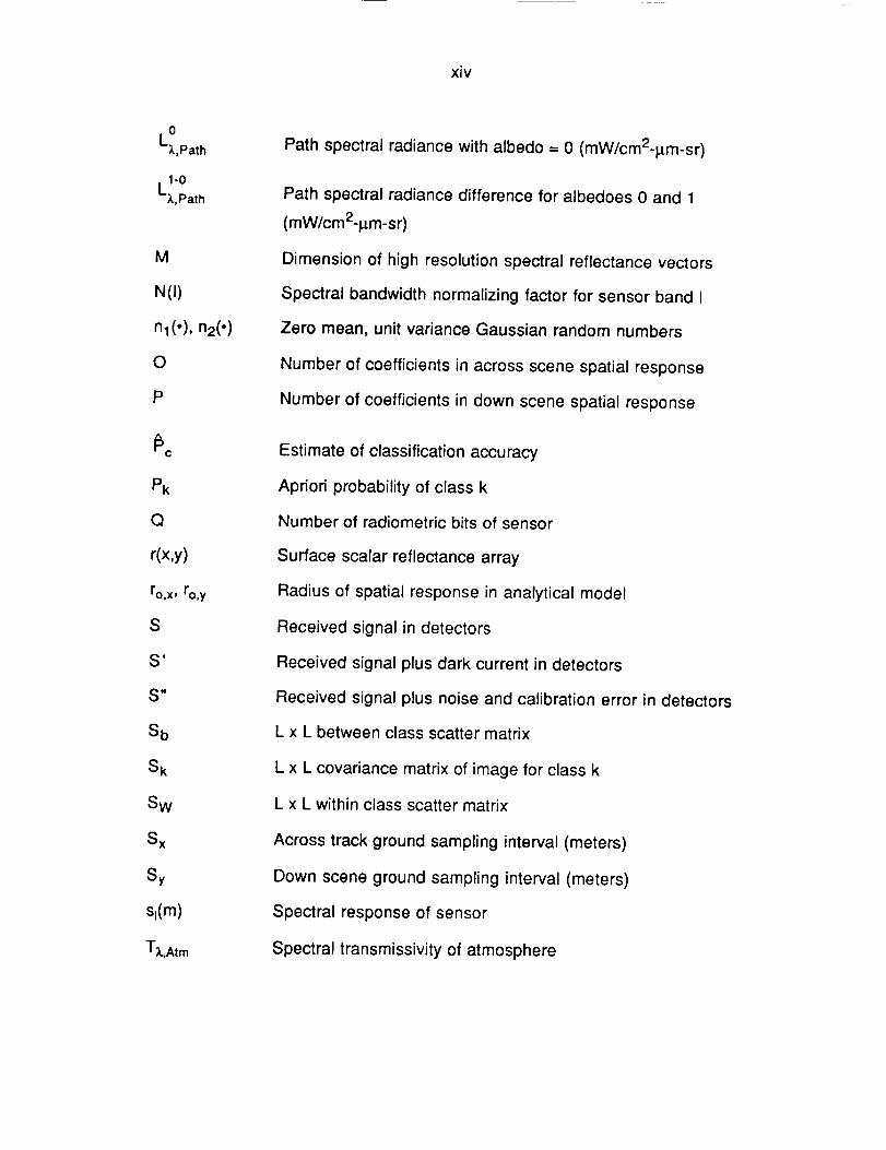
variations and states that contribute to the output of the system. Figure 1.3 is a
signal taxonomy of such effects.
These taxonomies offer a framework in which remote sensing system
effects can be grouped and located. The categories under the main
subsystems delineate sources of major contributions to the system state. In
some cases, effects or sources are listed in both signal and noise structures.
These dual listings exemplify one of the major problems in understanding
remote sensing systems. Depending on what type of information is desired,
sources or effects may indeed represent both noise and signal effects.
After the system has been broken down into identifiable portions, one
can take these blocks and build them back up into an overall system model.
Through the synergism possible from this combination of models and their
application the overall understanding of the entire process can be improved.

Chapter 1 - Introduction 6
01-.
_==_.,,=,
LI. D
rcu.
¢-_ , w,<
I
(/) I
UJ II
0 | , , , ,
u I
"E _-
!°
zW
0
C
l.l-
,-n_-i
m
•- ._ ._ _ ._-
o o _ _ _ -_.Q 0 v'._ "i
' '> 0i
m C
_o 0----- _ _ _ __ "_ _" 0 Or) O_
230
0Z
U-
7 Chapter 1 - Introduction
t31--ZZ
co>-_i,,. rv-
mu.
coco
cocoiii00Iz:o,.
rr I m0 Ico iZ Iu.I Ico I i
m
ua iZ Iw =tj ICO I--
mlmmml
J
I U)
I )_i _ [TJ
__[--,-iI C "--
m i
23
9-
0
m
E _
0m
E
m
co
mi
m ,m i
u i
I ,m i
mm
¢U
0n
,i-,0
Q
u.Im
¢" C
I t
i
: . __ o8_ _
_, CO I-<{i i
IT'
__.%.J ,
8
.-_ _¢- "E
¢-
230
f--
if)
U_

Chapter 1 - Introduction 8
1.3 Related Work
The systems approach to the remote sensing process has been of
interest for many years. In a tutorial paper by Landgrebe (1971), the differences
between image based (photogrammetry) and numerically oriented remote
sensing systems were described. The important factors to consider from an
information point of view were delineated and described. The work described
there helped to shape the ideas that are implemented in this research.
There have been many previous optical system simulation studies
reported in the literature, including those done in the context of civilian remote
sensing and those in a military context. Table 1.1 provides an overview of such
studies including the reference and key characteristics of each.
Those studies fall into one of three categories: Landsat TM sensor
parameter studies, basic parameter studies, and military studies. The Landsat
TM sensor parameter studies were performed in preparation and analysis of the
performance of Landsat-D Thematic Mapper. The basic parameter studies are
ones that are most closely related to what the research in this report considers.
They represent studies showing the tradeoffs of various system parameters and
their effects on some output measure, usually classification error. A few military
system studies are included to represent the unclassified literature in optical
system simulation.
The combination of several characteristics of the research presented in
this report distinguishes it from these previous studies. It presents a
sophisticated framework in which detailed models of the various components of
the system may be implemented. Flexibility has been built in to allow for
expansion and growth. High spectral resolution has been used throughout the
model in simulating the next generation of imaging spectrometers. Models from
the scene, the sensor, and the processing portions have been integrated to
create the ability to study cross system parameter interrelationship effects on the
classification and noise performance. All of these features together make it an
unique contribution to remote sensing science.

9 Chapter 1 - Introduction
°mlo
O3t-o
°m
"-5E
o3
._e
..o
I-
L
8 8 -8
,., 8 8.__ ._ .__
rr n'- ¢r
selPnl$ I_11 selpnls Je]etueJe d olse 8 _._e|llll N

Chapter 1 - Introduction 10
1.4 Report Organization
In this chapter, the objectives of the research were stated as being to
document, model, and investigate the effects of various remote sensing system
parameters on system performance. Also, the concept of a remote sensing
system was defined. Chapter two discusses models and algorithms useful in
simulating the remote sensing system process. Chapter three presents an
alternative system model based on a parametric description of the system state,
using analytical equations to describe the effect of the various system
components. Chapter four presents results of applying these models to various
system configurations based on an imaging spectrometer and studying the
effect of system parameters on noise and classification performance. Chapter
five concludes the report by discussing the results of these studies and possible
future extensions of the work.

11 Chapter 2 - Remote Sensing System
Modeling and Simulation
CHAPTER 2
REMOTE SENSING SYSTEM MODELING AND SIMULATION
2.1 Overview of System Model
In the modeling of a complex process, the goal is often to represent the
process faithfully while reducing the complexity of the description. In the
development of a model, we observe the process, take data measurements,
and formulate an abstraction from these observations and data. This model
then describes the process under varying conditions without having actually to
duplicate it. Thus, the model serves as a documentation of our understanding
of the process, as well as a tool useful in gaining insight into its operation. The
models presented in this chapter serve both of these purposes.
The modeling of a system may be done at many levels of abstraction.
The lowest level is the system itself. However this represents little knowledge of
the system and is often impractical to use in studying its operation. The next
level is with the use of detailed models of system components and simulation of
the system operation. This chapter discusses component models useful in such
a simulation. A still higher abstraction is a parametric and analytic description
of the system. Chapter three presents a system model based on this type of a
description.
The modeling of an optical remote sensing system is challenging
because of its complexity. However, through the use of the taxonomies
developed in the previous chapter this can be reduced to a manageable task.
In chapter one the remote sensing process is described as a system and further
divided into three subsystems: the scene, the sensor, and the processing
subsystems. Figure 2.1 shows this division in the context of a system model that
is described in this chapter for the simulation of the remote sensing process.

Chapter 2 - Remote Sensing SystemModeling and Simulation
12
O:E
o
E
e'-
e-
if)
0E
rr
u.

13 Chapter 2 - Remote Sensing SystemModeling and Simulation
The following sections detail the models used for the scene, the sensor,
and the processing subsystems. In each section various approaches to
modeling or describing the processes involved are discussed. Section 2.2
discusses considerations in modeling the surface reflectance and the
atmospheric effects and presents the model used in this report for simulating the
scene. Section 2.3 describes the effects on the scene radiance introduced by
the sensor, in both the remote sensing process and the simulation. Section 2.4
discusses approaches to extracting information from a multispectral image, as
well as describing the options available in the simulation. Section 2.5
summarizes the models presented in this chapter.
2.2 Scene Models
The scene subsystem is by far the most complex, varied, and unknown of
the remote sensing process. It is understood that no model can accurately
represent all of the complex variations that make up the spectral radiance
present at the input of the sensor. However, through the use of various
simplifying assumptions, developing such a model becomes a reasonable task.
In this section, approaches to modeling the scene are discussed.
From the taxonomies of chapter one, the scene is seen to consist of the
solar illumination and atmospheric effects, the surface reflectance, and the
goniometric effects due to the angles of illumination and view. In developing a
model for the scene, models for the solar illumination and atmosphere, along
with the surface reflectance are used, while the goniometric effects are
embedded within the relationships between these two components. Figure 2.2
presents a block diagram of the basic scene model structure.
SolarIllumination
Surface
"- Reflectance vi
UpwardAtmospheric
Effects
Figure 2.2 Scene Model Block Diagram.
Chapter 2 - Remote Sensing System 14Modeling and Simulation
To further describe the modeling of the scene, the rest of this section is
divided into two parts. Section 2.2.1 discusses modeling of the surface in
general terms, as well as describing in detail a model used to simulate the
surface reflectance. Section 2.2.2 then discusses the solar illumination and the
atmospheric effects present in optical remote sensing systems and their
simulation implementation.
2.2.1 Surface Reflectance Modeling
In this section various methods of representing the reflectance of the
surface are presented. The discussion begins with the most general way of
describing this reflectance, followed by approaches using deterministic canopy
models, and then concludes with models developed from the statistics of field
reflectances. The model chosen for implementation in the simulation is then
discussed.
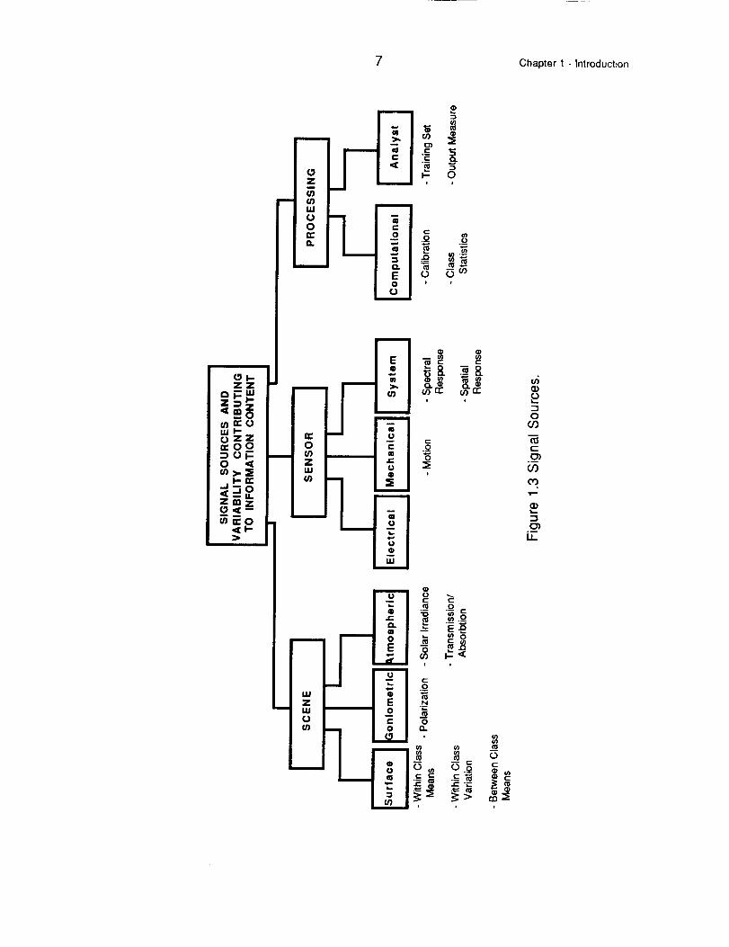
The most general measurement of the reflectance of a surface is given by
the Spectral Bidirectional Reflectance Distribution Function (SBRDF). This
function is defined (chapter two of Swain and Davis, 1978) as in equation 2.1.
P_.(esolar,$solar, eview,$view) = dLx(eview'$view) sr-1dE;_(esoJar,_solar )
(2.1)
Here, L_.(0view,(_view) is the reflected spectral radiance observed at angles
eview, _view, and Ex(esolar,$solar ) is the incident spectral irradiance at angles
esolar, _)solar. The geometry used here and in the rest of the report is shown in
Figure 2.3.

15 Chapter 2 - Remote Sensing System
Modeling and Simulation
Z
t0 o-
solar
Figure 2.3 Scene Geometry.
The quantities {)solar and 0view are the zenith angles as measured from
local vertical, while (_solar and Cview are the azimuthal angles as measured from
North on a map.
The SBRDF gives the reflectance of an object from all angles of
incidence and view and thus is the most complete representation of the surface
reflectance. However, the accurate measurement of the SBRDF is a difficult
task and few studies have been made.
A problem in obtaining the SBRDF arises due to spatial considerations.
Typically, in remote sensing applications the scene is sampled spatially across
two dimensions at some surface cell size G x by Gy. A rectangular coordinate
system is overlaid and an aggregate reflectance is obtained over each
individual cell at spatial location (x,y). An aggregate SBRDF is then a function
of not only the geometry involved, but also the surface resolution cell size, the
location in the scene, and the various materials contained within the cell.

Chapter 2 - Remote Sensing System 16Modeling and Simulation
Aggregate SBRDF = p_.,ag(Gx,Gy,x,Y,esolar,_)solar;eview,(I)view) (2.2)
Since the surface cell size Gx by Gy may be a number of meters square
in typical remote sensing data sets, the measurement of the aggregate SBRDF
on the surface is very inconvenient. Shibayma and Wiegand (1985) and Irons,
Ranson, and Daughtry (1988) have reported some measurements of this type,
but for limited crop species and over few wavelength intervals.
Thus, while the use of the measured SBRDF is the most complete way of
representing the reflectance of the surface, it is impractical to use because of
the difficultly in obtaining complete data for various cover types.
Strahler, Woodcock, and Smith (1986) discussed modeling of the scene
for land resource remote sensing applications and divided surface models into
two types: deterministic canopy models and stochastic image processing
models. The term canopy comes about because these models attempt to
calculate the SBRDF of vegetation by using radiative transport theory.
Differential equations are used to compute the reflectance/transmittance of the
several layers of leaves in a vegetative canopy.
Some examples of canopy models are the AGR model (Allen, Gayle, and
Richardson 1970), the Suits model (Suits 1972a) with extensions for azimuthal
(Suits 1972b) and row effects (Suits 1982), the SAIL model (Verhoef 1984), and
the models by Park and Deering (1982), Cooper, Smith and Pitts (1982), and
Kimes and Kirchner (1982). All of these models are based upon having precise
knowledge of the reflectance, transmittance, and orientation of the leaves in
each layer of the canopy. A model that used probability distributions in
describing the orientations of the layers was described in Smith and Oliver
(1974).
All of these canopy models, however, only consider the reflectance within
a single surface cell, assuming the entire area covered by a particular surface
type is homogeneous and with no regard to the spatial variability typical of
almost all remotely sensed scenes. While they are capable of accurately
modeling the SBRDF of a particular surface material, their lack of spatial

17 Chapter 2 - Remote Sensing System
Modeling and Simulation
information limits their applicability for the type of system study undertaken in
this research. However, it certainly would be conceivable, if one had the
appropriate data, to extend a canopy model to be able to contain spatial
information and develop a very accurate surface reflectance model.
Unfortunately, this type of detailed database does not exist at the present time.
Image processing models, on the other hand, are not concerned with the
reflectance structure within a scene resolution cell, but rather how the
reflectances vary spatially and spectrally from cell to cell. In these models, the
spectral reflectances of a surface area are taken to be multidimensional (across
the spectral domain) random vectors with spectral and spatial correlation.
While these models are usually developed from imagery that represent the
radiance over an area, it can be assumed that the reflectances of the surface
cells vary similarly in the spatial sense as do the image pixels. Also, the
reflectance within each cell is assumed to be independent of illumination or
viewing angle. This is known as Lambertian reflectance (Swain and Davis,
1978).
In the use of image processing models for the surface reflectance two
assumptions are generally made about the spectral and spatial variation in the
scene. The multispectral reflectance vectors are usually assumed to be
samples from an M-dimensional multivariate normal (or Gaussian) probability
distribution function. The form of this distribution is shown in equation 2.3.
/
p(x ,x2,...,xM) = ( )M( /1221)
Here, X={xl,x 2 ..... XM)T data vector, X is the mean vector, and ,_, is the
covariance matrix.
The work that is often cited in justifying this assumption is that of Crane,
Malila, and Richardson (1972). They worked with 12 band MSS data that was
transformed to its principle component space and reduced to three bands.

Chapter 2 - Remote Sensing SystemModeling and Simulation
18
Since the transformation produces uncorrelated variables, they tested each of
the three bands for goodness-of-fit to Gaussian random variables. While the
results showed a fairly good fit to the univariate Gaussian model, they ignored
the fact that just because these random variables were Gaussian, that did not
mean that the original 12 dimensional random vectors were multivariate
Gaussian. This comes about because of the fact that combining Gaussian
random variables into a vector does not necessarily result in jointly Gaussian
random vectors. A much better test would be to use the procedures discussed
in Koziol (1983) or Smith and Jain (1988) to check for multivariate normality.
Some early work done at LARS found the Gaussian assumption not to
hold under the Chi-Square goodness-of-fit test. Members of the LARS Staff
(1969) found that the Gaussian assumption did not hold for several
multispectral data sets gathered from an airborne scanner. The results of this
study may have been affected by the particular data they considered, or even
the histogram cell interval used in the distribution test.
Nevertheless, the Gaussian assumption results in much simpler
methods of generating and analyzing the data than those based upon more
accurate, yet computational complex models.
Remotely sensed images have also been shown to have a pixel to pixel
spatial correlation. Kettig (1975) used this fact in development of the ECHO
spatial classifier. Also, Mobasseri (1978) developed a multispectral spatial
model that was a separable (across and down scene) exponential model. This
spatial model used by Mobasseri is specified by its spatial autocorrelation
function Rmm('_,T1) for the scene reflectance rm as given in equation 2.4.
- a_ - br_l_qlE{ rm(X+l:,Y+TI) rm(X,Y) } = Rmm(l:,Tl) = e e (2.4)
Here, a m and bm are the across scene and down scene correlation
parameters for wavelength m, and '_ and 11 are the respective scene cell lag
values. The coordinates (x,y) are the scene cell location.

19 Chapter 2 - Remote Sensing SystemModeling and Simulation
Equation 2.4 may also be written in terms of the autocorrelation
coefficients, Px = ea and py = e-b, as in equation 2.5.
Rmm(,_,_) p-I_l -Illl= m,x Pm.y (2.5)
This form of autocorrelation for a random field is equivalent to that of a
wide-sense Markov random field with the neighbor set consisting of the quarter-
plane causal neighbors, {(0,-1), (-1,0), (-1 ,-1)} (chapter seven of Rosenfeld and
Kak, 1982). This is also equivalent to a two-dimensional autoregressive (An)
model (Delp, et al., 1979) as given by equation 2.6.
r(x,y) = C1 r(x-l,y) + 02 r(x,y-1) +C3 r(x-l,y-1) + _u z(x,y) (2.6)
Here,
x,y - high resolution spatial column, row index in scene
C1 = Px
02 = py
C3 = "PxPy
_u - standard deviation of Gaussian driving process, computed to retain
unit variance for r (See algorithm given in Appendix A)
z(x,y) - independent Gaussian random numbers with unit variance and
zero mean.
Given arbitrary initial conditions, the AR model can easily generate a
reflectance array with the desired spatial correlation. Other methods also exist
to generate a random field with the spatial model of equation 2.4. Mobasseri
(1978) used a Fourier-based technique, and Chellappa (1981) studied methods
of generating spatially correlated arrays using arbitrary neighborhoods.
Using the Least Squared Error (LSE) estimation technique for the AR
coefficients as described in Delp, et al., (1979) some typical coefficients for the
AR model were calculated. Table 2.1 shows these typical values of the spatial
parameters for a variety of scene types, computed from a line scanner image ofan infrared band.

Chapter 2 - Remote Sensing System 20
Modeling and Simulation
Table 2.1 Typical Spatial Model Parameters.
Full cover vegetationJust emergent row crops
Bare soil field
C 1=0.63 C2=0.55 C3= -0.35
c1=0.63 c2=0.70 c3=-0.44c1=0.57 c2=0.72 c =-0..41
A problem with using line scanner imagery to compute the spatial
statistics is that there is correlation introduced by the instrument itself, and as a
result, computing the statistics from the image data does not truly represent the
correlation of the original scene. This is difficult to prevent, as with any imaging
sensor this effect will be present. It is known, however, (Papoulis, 1984) that the
output correlation is greater than the input correlation for a linear system with
the response similar to imaging systems. Thus, one can reasonably assume
that the actual pixel to pixel correlation of the original scene was slightly less
than that which was computed from the imagery.
An alternative method of gathering data to estimate spatial correlation is
to use an instrument such as the Field Spectrometer System (FSS) described in
Hixson, et al., (1978). With this instrument, spectral reflectance measurements
were made with a spectral resolution of approximately 20 nm, and a ground
field of view of approximately 25 meters. The instrument was mounted in a
helicopter and flown over fields at a height of approximately 60 meters. The
instrument made spectral radiance measurements that were converted into
reflectance by comparison to the radiance measured over a known calibration
panel. The report by Biehl, et al., (1982) describes the database of reflectance
data measured by this and other instruments.
A comparison of the spatial correlation of imagery and spectrometer
samples was made for two fields from Hand County, South Dakota. Both
aircraft line scanner imagery and FSS reflectance data were obtained over
fields 168 and 288 on July 26, 1978. Field 168 was mostly bare soil, while field
288 was ripe Millet with nearly 100% ground cover. The spatial correlation of
the imagery was done in the same direction and over the same area that the
FSS had acquired data. The direction was along the flightline for both
instruments. Since the aircraft imagery had a ground field of view of

21 Chapter 2 - Remote Sensing SystemModeling and Simulation
approximately eight meters, the correlation coefficients for the aircraft imagery
were calculated at both one and three pixel lag values to be able to compare
the coefficients with those of the FSS at a similar intersample distances. The
correlation coefficients are computed with the estimate given in equation 2.7.
=
N-1
n=l
(2.7)
(Xn.n=l
Here, '_ is the lag value, N is the number of data samples and Y is the
sample mean. Table 2.2 shows the spatial correlation coefficients for two
wavelengths in each field and two pixel distances of the aircraft scanner.
Table 2.2 Spatial Correlation Coefficients for Hand County, South Dakota.
Field Wavelength Aircraft Aircraft FSSNumber 8 Meters 24 Meters 25 Meters
168
Bare Soil
0.56 p.m 0.82
1.00 Ilm 0.87
288 0.56 _m 0.61
Ripe Millet 1.00 _m 0.67
0.31
0.53
0.44
0.20
0.28
0.48
0.25
0.16
The results of Table 2.2 show that as the distance between samples
increase, the correlation coefficient decreases. Also, there seems to be a
significantly higher correlation among the imagery pixels as compared to those
of the spectrometer, even when they are computed using samples a similar
distance apart. Thus, there does appear to be an increase in the correlation
coefficient due to the characteristics of the line scanner.

Chapter 2 - Remote Sensing System 22Modeling and Simulation
To investigate the typical variation of the correlation across the spectrum,
the spatial correlation coefficient was computed from some FSS data of a winter
wheat field (number 151) from Finney County, Kansas taken on May 3, 1977.
The wheat was beginning to ripen and there was approximately 30% ground
cover. There were 58 samples across the field, each about 20 meters apart.
The correlation coefficient for "c=1 as calculated in equation 2.7 for each
wavelength is shown in figure 2.4.
G)0
om
o0
¢,-,o
L--L--
o0
1.0
o.g
0.8
0.7
0.6
0.5• I • | •
0.4 0.6 0.8• • • | • | • • •
_0 '2 =41 1. 1. 1.6 1.8 2'.0 2_2 2.4
Wavelength
Figure 2.4 Correlation Coefficients of Winter Wheat Field.
The large peak around 1.4 and 1.9 t_m is due to substituting 0.1% for the
reflectance in the water absorption bands of the data. The other large peaks
are also due to atmospheric absorption bands. The flat segments are from
repeated values used in the plot due to the uneven spectral sampling of the
FSS. For most of the wavelengths the correlation coefficient ranges around
0.85. This correlation among samples is significantly higher than those of Table

23 Chapter 2 - Remote Sensing SystemModeling and Simulation
2.2. This is indicativ_ of the high variability in correlation among surface cover
types and conditions.
While the exponential model is one way of modeling spatial correlation,
spatial models based on fractal geometry (Mandlebrot 1977, 1982, Gleick 1987,
and Peitgen and Saupe 1988) have emerged as a powerful method for
modeling natural phenomena. This is partly because its mathematical
construction is similar to what is observed in natural scenes. In two spatial
dimensions, the fractal random field r(x,y) has the property shown in equation
2.8, where D is the fractal dimension (2<D<3).
fE I r(x2'Y2) " r(xl'Yl) o_ _ (x 2 - xl) + (Y2- Yl ) (2.8)
That is, the variance of the difference between pixel locations is
proportional to the distance raised to a fractional power. Several experiments
were conducted to measure the fractal dimension of typical agricultural scenes.
Values for D ranged around 2.6_+0.1 for several cover types. See Dodd (1987)
for an example in using fractal concepts to generate multispectral texture by
computing the fractal dimension D from principle component images.
While several methods have been discussed for generating scenes with
spatial correlation, the autoregressive model was chosen for implementation in
the simulation. This model is efficient in generating a simulated reflectance
array using computer-generated random numbers. Table 2.3 presents an
overview of the technique used to simulate the surface reflectance, while the
paragraphs following describe these steps in detail.

Chapter 2 - Remote Sensing System
Modeling and Simulation
24
Table 2.3 Sequence in Generating a Simulated Surface Reflectance Array.
Step 1. Define scene size and class boundaries.
Step 2. Obtain spatial and spectral statistics ofreflectance data for each class.
Step 3. Generate spatial correlated reflectancearrays for each wavelength, with each arraybeing spectrally uncorrelated.
Step 4. Transform each reflectance vector to have
the proper mean and covariance for theappropriate class.
Step 5. Interpolate resulting spectral reflectancevector to the desired spectral resolution ofscene.
The scene is first defined by determining its size, X columns by Y rows,
where each location (x,y) is a square scene cell with the distance on one side
specified in meters. Each of these scene cells are assigned to one of the K
classes. Class boundaries are specified by the upper left index and lower right
index of the rectangular area containing the class.
Reflectance data for each class used in the simulation is obtained from
the database of FSS measurements. Over the wavelength range considered in
this report there are 60 wavelength samples in the FSS data. Thus, the spectral
statistics are 60 dimensional. The across scene and down scene spatial
coefficients are estimated from imagery over scenes similar to the one being
simulated. Typically, the same spatial correlation is assumed for each
wavelength, while no wavelength-to-wavelength spatial crosscorrelation is
specified.
The AR model is used to generate the spatially correlated reflectance
cells within the area defined for each class k, and for each wavelength band m
as shown in equation 2.9,

25 Chapter 2 - Remote Sensing System
Modeling and Simulation
rm(X,Y) = Px rm(X-1 ,Y) + Py rm(X,y'l) " PxPy rm(x'l ,y-l) + Ou z(x,y) (2.9)
where the symbols are defined as in equation 2.6.
The individual arrays {rm(X,y)} are arranged as a spectral vector array,
{R(x,y)}. Reflectance data of each class k are used to compute the mean vectors
ek and covariance matrices _k. The eigenvalues and eigenvectors of these
covariance matrices are then computed and arranged as diagonal matrices ,A,k
and column matrices (_k, respectively. The surface reflectance array {P(x,y)} is
then obtained by using equation 2.10, where for each scene cell location (x,y)
the appropriate class transformation is applied.
1
2
P(x,y) = Pk + C_)k Ak R(x,y)(2.10)
The resultant reflectance array will be multivariate Gaussian with the
mean and covariance of the original class statistics, and be spatially correlated
according to the exponential model of equation 2.4.
While the FSS reflectance data covers the entire range from 0.4 to 2.4
pm, the wavelength sampling is uneven, ranging from 20 nm to 50 nm. In order
to have a uniform spectral resolution for the scene model, an interpolation is
performed on each spectral reflectance vector to yield 201 wavelengths spaced
at 10 nm intervals. The algorithm used to perform this interpolation is given in
Appendix B.
2.2.2 Solar and Atmospheric Modeling
In this section, the modeling of the solar illumination and the atmospherio
effects present in optical remote sensing systems is discussed. Following a
preliminary list of references to work in this area, a general model of the
atmosphere is presented. This is followed by a discussion of measures of
atmospheric quality. The model used in the simulation is then presented, along
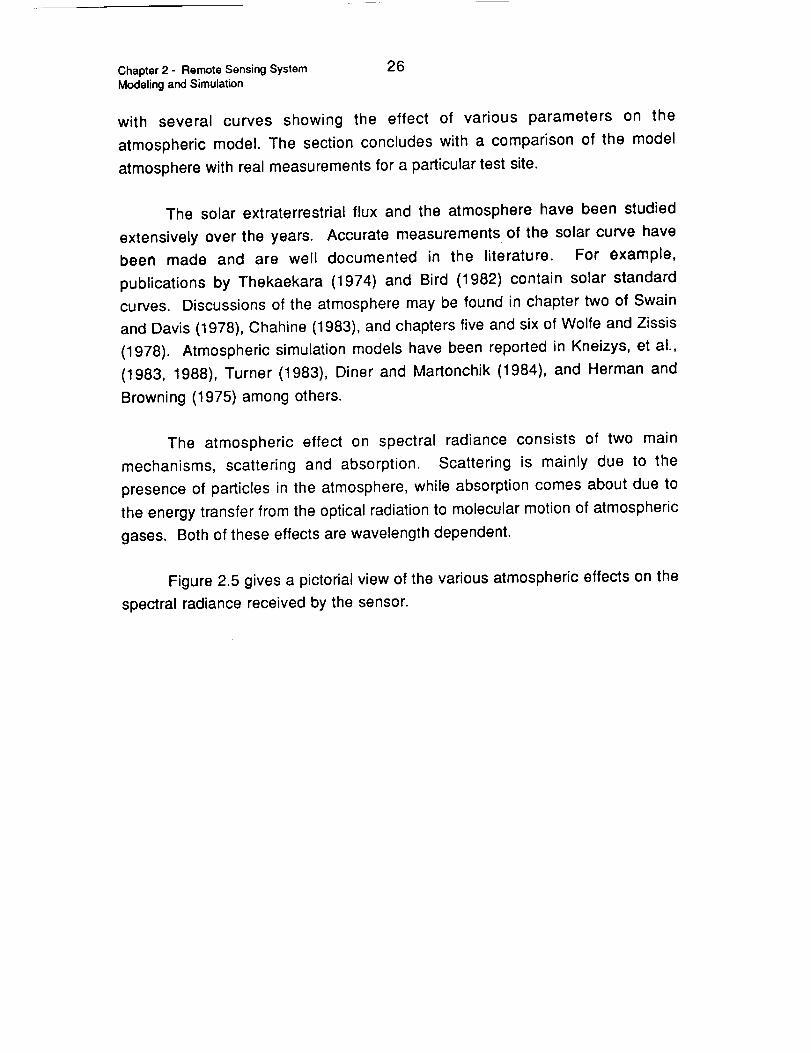
Chapter 2 - Remote Sensing System 26Modeling and Simulation
with several curves showing the effect of various parameters on the
atmospheric model. The section concludes with a comparison of the model
atmosphere with real measurements for a particular test site.
The solar extraterrestrial flux and the atmosphere have been studied
extensively over the years. Accurate measurements of the solar curve have
been made and are well documented in the literature. For example,
publications by Thekaekara (1974) and Bird (1982) contain solar standard
curves. Discussions of the atmosphere may be found in chapter two of Swain
and Davis (1978), Chahine (1983), and chapters five and six of Wolfe and Zissis
(1978). Atmospheric simulation models have been reported in Kneizys, et al.,
(1983, 1988), Turner (1983), Diner and Martonchik (1984), and Herman and
Browning (1975) among others.
The atmospheric effect on spectral radiance consists of two main
mechanisms, scattering and absorption. Scattering is mainly due to the
presence of particles in the atmosphere, while absorption comes about due to
the energy transfer from the optical radiation to molecular motion of atmospheric
gases. Both of these effects are wavelength dependent.
Figure 2.5 gives a pictorial view of the various atmospheric effects on the
spectral radiance received by the sensor.

27 Chapter 2 - Remote Sensing SystemModeling and Simulation
Surlace
Figure 2.5 Atmospheric Effects on Spectral Radiance Received by Sensor.
From this figure, several main factors are seen to contribute to the
radiance received by the sensor. The exoatmospheric spectral irradiance,
E_.,Exo, is attenuated and scattered by the atmosphere before reaching the
surface as the direct spectral irradiance E_.,Direc t. Some of this scattered
radiation also reaches the surface as E_.,Diffuse, the diffuse spectral irradiance (or
skylight irradiance.) The reflected spectral radiance L;_.,Surface passes through
the atmosphere and is attenuated by the spectral transmittance T_.,Atm of the
atmosphere. Also, some of the solar irradiance that is scattered by the
atmosphere finds its way into the sensor field of view as L_.,eat h, the path
spectral radiance. This path radiance also includes that which may have been
reflected off of the nearby surface (adjacency effect) before being scattered into
the sensor field of view, as well as the background radiation of the atmosphere.
These factors contribute to the spectral radiance of the scene, as
received by the sensor, in a manner described by equation 2.11.

Chapter 2 - Remote Sensing SystemModeling and Simulation
28
1Fcos(e , ) +E 1L_,sensor = -_-_. solar E_,,Direct _,,DiffuseJ Rz T;L, Atm + L_Pat h (2.1 1 )
Here, R x is the spectral reflectance of the surface. In the most general
sense it is the Spectral Bidirectional Reflectance Factor (SBRF) that gives the
reflectance for all angles of incidence and viewing. The other factors also
depend upon the angles of illumination and viewing as well as the quality of the
atmosphere.
Several other important aspects of the real atmosphere also influence
the values in equation 2.11. One is the spatial dependence of the atmospheric
scattering and absorption effects. The make-up of the atmosphere is not
constant over a scene; however, it is unclear how the atmosphere changes from
pixel to pixel over typical pixel sizes (20-30 meters), and is usually assumed to
be constant. Another spatial effect of the atmosphere is the blurring that can be
introduced by the scattering in the atmosphere. Kaufman (1985) has studied
the atmosphere from this point of view, suggesting that the atmosphere be
modeled with a spatial modulation transfer function (Goodman, 1978) similar to
those used in the modeling of sensors. This could be implemented in the model
in a spatial convolution with the scene radiance. Yet another effect that is often
ignored is the time dependence of the atmospheric effects. Fast moving gases
exist in the upper atmosphere and cause a changing effect on the scattering
and absorption over the field of view of the sensor. The movement of clouds is
an example of this time dependence.
The quality of the atmosphere may be represented by several different
measures. The fundamental parameter for atmospheric quality is the spectral
optical thickness "_z. The spectral transmittance TZ,At m of the atmosphere
between two points x 1 and x 2 is defined by equation 2.12 where J3(X,z) is the
volume extinction-coefficient with units of Km "_.

29 Chapter 2 - Remote Sensing SystemModeling and Simulation
[xf]T_.,Atm = exp - _(;L,z) dz (2.12)
The integral inside the exponent of this equation is known as the spectral
optical thickness 'ck and is defined in equation 2.13.
X2
= 113(k,z) dzQ#
X I
(2.13)
Visibility is also often used as a measure of the clarity of the atmosphere
and is defined (Kneizys, et al., 1983) by "the greatest distance at which it is just
possible to see and identify with the unaided eye in the daytime a dark object
against the horizon sky." The surface meteorological range Vn is related to
visibility (usually by a factor of 1+0.3), but defined numerically, rather than by
subjective judgement. For the typical atmospheres used in this report, it is
assumed that the two terms can be used interchangeably. Surface
meteorological range is related to the volume extinction-coefficient at k=0.55
pm through equation 2.14.
Vn- 3.912 Km (2.14)_X=0.55
Surface meteorological range (or visibility) is the measure commonly
used in remote sensing for atmospheric quality. However, some experiments
specify the optical thickness (also called optical depth for a vertical path). Data
from Elterman (1970) was used to find an empirical relationship between optical
thickness and visibility. Figure 2.6 shows points from Elterman's data along
with a best fit curve. These data points are for k = 0.55 #m. Optical thickness is
also dependent upon wavelength. Data from EIterman (1968) was plotted in
Figure 2.7 along with a best fit curve for the empirical data. This relationship is
for a surface meteorological range of 25 Km.

Chapter 2 - Remote Sensing System
Modeling and Simulation
3O
2,0 ,
1.9-
1.8-'
o) 17 _¢_
16-1.8;
"_ 1.4"
__. 1.321.2-'
1.1
_a. 1.o;
0 o.9-0.8-
0.7-
0.6-_ 0.5-
_ 0.4-UJ 0.3-
0.2-
0.1-
0.0
Optical Thickness vs. Visibility
from Elterman (1970)
y. 2.7534 " x^-0.65576 R^2 - 0.997
i - l - i - i - i - i - i - l - i
5 10 15 20 25 30 35 40 45
Visibility (Km)
5O
Figure 2.6 Optical Thickness '_ vs. Visibility.
2.0
1"9 1
1.8
1.7
1.6
Optical Thickness vs.Wavelength from Elterman (1968)
y = 0.17628 * X^-1.3280 R*2 = 0.967
¢0 1"5 1
1.4Oe.- 1.3J¢ 1.2tJ
1.1-1.0"
0.9"0 0.8
0.6
0.5
0.4
0.3
0.2
0.1
0.0o, o_6 o_8 1'o
Wavelength (microns)
b _
.2
Figure 2.7 Optical Thickness vs. Wavelength.

31 Chapter 2 - Remote Sensing SystemModeling and Simulation
These empirical relationships were used to derive equation 2.15 relating
spectral optical thickness to meteorological range and wavelength.
'{x(V.q) = 1.35k'l'328V_q 0'656 (2.15)
This equation is assumed to be valid only over optical wavelengths and
meteorological ranges from 2 to 50 Km.
In this research the solar and atmospheric model is implemented with the
use of the computer code LOWTRAN 7 (Kneizys, et al., 1988). The program
LOWTRAN has evolved over the years from simply an atmospheric
transmittance code to one that is now capable of computing direct solar
irradiance and multiply scattered atmospheric radiance.
LOWTRAN uses radiative transfer theory to compute the transmittance
and radiance in each of 32 layers of the atmosphere. Well documented data
tables embedded within the program give accurate spectral transmittance and
radiance values at minimum wavenumber intervals of 20 cm -1. This model
compares favorably to ones developed by Diner and Martonchik (1984), and
Herman and Browning (1975), because of its continuous spectral coverage and
its inclusion of narrow absorption bands due to the various constituents of the
atmosphere. A partial list of controllable parameters for LOWTRAN 7 is
contained in Table 2.4.
Table 2.4 Example LOWTRAN 7 Parameters
Solar positionMeteorological rangeSurface albedo
Atmospheric hazeAltitude of observer
Zenith angle of observer
!Wavelength range and increment

Chapter 2 - Remote Sensing System 32Modeling and Simulation
LOWTRAN 7 is used along with the models discussed below for the
diffuse irradiance and path radiance to compute the radiance received by the
sensor. Appendix C contains the input file format used in the calls to
LOWTRAN.
The spectral radiance present at the input to the sensor model in the
simulation program is computed as in equation 2.16.
1L_.,Sensor (x,y) = _- E_,TotaI P(x,y) TAt m + L;_,Path (2.16)
The generation of the three atmospheric components of this equation is
discussed below, while the spectral reflectance array P(x,y) is as calculated in
section 2.2.1.
1. Total Spectral Irradiance. This is the total downwelling spectral
irradiance E_.,Total that is incident at the surface, and is equal to the sum of the
direct and diffuse irradiances as shown in equation 2.17.
E_.,Total = COS(esolar) E_.,Direct + Ex, Diffusa (2.1 7)
Since LOWTRAN does not have an option to generate the diffuse
component, a model was obtained from Chahine (1983). There, the total
surface spectral irradiance EX,TotaI is shown to be related to the direct spectral
irradiance through the curve given in Figure 2.8. Also shown in the figure is an
exponential model derived from the data.

33 Chapter 2 - Remote Sensing SystemModeling and Simulation
I,U
.="ouJ
1 _0
I "._, _ Data
0'8 IJ """,_ .... Exponential Modet
0.6. _%
0.4. '_,_
0.2. _'
0.0oo ols ,io " 11s 2'o 30
Total Optical Path Length
Figure 2.8 Ratio of Direct to Total Irradiance vs. Total Optical Path Length.
The total optical path length "Cp,;_is related to the optical thickness by
multiplying by seC(esolar) as in equation 2.18.
'tp,_.(Vq,esolar) = '_x(V_l)sec(esolar) (2.18)
This relationship between direct and total irradiance is given as a
function of the total optical thickness of the atmosphere in equation 2.19. Thus,
equation 2.19 can be used in conjunction with equation 2.15 to obtain the total
surface spectral irradiance from the direct spectral irradiance, the surface
meteorological range, the diffuse irradiance constant, and the solar zenith
angle.
Ex, TotaI (V_], (_solar) =
COS((_solar)Ex.,Oirsct (V_q, esolar)
exp[ "KD I:_.(V_)sec((_solar) ]
(2.19)

Chapter 2 - Remote Sensing System 34Modeling and Simulation
The diffuse irradiance constant K D is dependent upon the type of
atmosphere and the overall surface reflectance. In the discussion by Chahine
(1983) from which Figure 2.8 was taken, the author stated that the curve was for
a nonabsorbing atmosphere and surface albedo < 15%. It was also indicated
that for absorbing atmospheres and higher albedoes the curve would be
steeper. While no specific values were given in the reference, Table 2.5 shows
some estimates of K D for different conditions. The model shown in Figure 2.8
was with KD = 0.73.
KD
0.730.841.001.26
Table 2.5 Diffuse Irradiance Constant Values.
Type of Atmosphere
nonabsorbingabsorbingabsorbingabsorbing
Surface Reflectance
low ( < 15%)low ( < 15%)
medium (15 - 30 %)high ( > 30%)
2. Atmospheric Spectral Transmittance. This is directly computed using
LOWTRAN for a path from the surface to the sensor. This may be a vertical or
slant path through the atmosphere, depending on the zenith angle of the
sensor. It represents the path loss due to scattering and absorption.
3. Path Spectral Radiance. This is computed by using two calls to
LOWTRAN. It is called once for a surface albedo of 0 and once for an albedo of
1. The total path radiance received by the sensor is then computed by
interpolating between these extremes as in equation 2.20, where (x,y,m)
specifies the spatial location x,y and wavelength m. pm,ave(X,y) is the average
surface reflectance for wavelength m in the neighborhood of x,y. In
implementing this model in the simulation the entire scene is used in computing
Pm,ave(X,Y).
• alb==O I alb=l alb=O "_L;L, Path(X,y,m) = L_.,Pat h (m) + Pm,ave(X,y) = L_.,Path(m) " L_.,Path(m) _ (2.20)

35 Chapter 2 - Remote Sensing SystemModeling and Simulation
This formulation of path radiance allows for its dependence on the
surface reflectance. This does not truly represent the situation in the real
system, as the path radiance there is dependent upon the reflectance of the
surface for each particular path the illumination follows before arriving at the
sensor, and there are many paths the illumination may take. However, this
simple linear model offers good compromise between accuracy and
computational complexity.
On the following pages, examples of how various scene parameters
affect these atmospheric model components. For these examples the default
parameters of Table 2.6 were used.
Table 2.6 Default Values of Atmospheric Parameters.
ParameterModel
Atmospheric HazeSurface Meteorological RangeDiffuse Irradiance Constant
Solar Zenith Angle
View Zenith AngleSurface Albedo
Default
1976 U.S. StandardRural Extinction16 Km0.73
30 °0o0.10
The following figures 2.9 through 2.14 show the direct, diffuse, and total
spectral irradiance for several meteorological ranges and solar zenith angles.
The curves for the diffuse irradiance were computed as the difference between
the total and direct spectral irradiances. Figures 2.15 and 2.16 show how
atmospheric transmittance varies for several meteorological ranges and view
angles. Figures 2.17 through 2.20 show how the path radiance component is
affected by meteorological range, solar angle, view angle and surface albedo.

Chapter 2 - Remote Sensing System 36Modeling and Simulation
A
c-oL_
E|
O4EO
E
o¢.,.
"Oe=
E
a,
12o.
lOO.
80
60
4o
20
0
0.4
32 Km
16 Km
........ 8 Km
....... 4 Km
........ 2 Km
!
0.6 0.8 1.0 1.2 1.4 1.6 1.8 2.0 2,2 2.4
Wavelength
Figure 2.9 Effect of Meteorological Range on Direct Solar Spectral Irradiance.
120
_'_ 0 Degrees
100 _ .............. 15 Degrees
........ 30 Degrees
....... 45 Degrees80
........ 60 Degrees
- - - - 75 degreesB
6O
• , I _,140 = r !
0.4 0.6 0.8 1,0 1,2 1.4 1.6 1.8 2.0 2.2 2,4
Wavelength
Figure 2.10 Effect of Solar Zenith Angle on Direct Solar Spectral Irradiance.

37Chapter 2 - Remote Sensing System
Modeling and Simulation
¢-
oo
E|
E
Ev
@tac¢gm"o(gl-
@O.
(t)
160,
140-32 Km
............... 16 Km
120 ........ 8 Km
....... 4 Km
100 _V"_ " - ....... 2Km
80
4o |
_o, _f'-.
o .. . /#/' -'=IkL _h.'..'-'_• • I • l • ! • l • = •0, o_6o_6 ,o ,2 1, 16 ,_ 2o 2.2 24
Wavelength
Figure 2.11 Effect of Meteorological Range on Total Solar Spectral Irradiance.
160Ac
.o0 140,
E' 120.
04__= _ 0 Degrees
...... 15 Degrees
........ 30 Degrees
E _M. ....... 4sDegrees
100 _j_.,_ ........ 60Degrees
8 ',IL,
40 ' ,
2o_m
_') 0 • i • J • i • B • • • • i--, "e •
0.4 0.6 0.8 1.0 1.2 1.4 1.6 1.8 2.0 2.2 2.4
Wavelength
Figure 2.12 Effect of Solar Zenith Angle on Total Solar Spectral Irradiance.

Chapter 2 - Remote Sensing System
Modeling and Simulation
38
5OAt-
O
E 40
¢_IE
E
oo 2Oc
_ 10
Qn
_' 32 Km
.............::mo4 Km
2 Km
0 • i • | • i • | -_ " i
• i " i0.4 0 6 0.8 1.0 1.2 1.4 1.6 1.8 2.0 2.2 2.4
Wavelength
Figure 2.13 Effect of Meteorological Range on Diffuse Solar Spectral Irradiance.
p,
oo
Ei
E
Ev
m
¢t)
5O
4O
3o
20
lO
0 Degrees
............... 15 Degrees
30 Degrees
L 45 Degrees
60 Degrees
75 Degrees
O • • • " , _ • a . a
0.4 0,6 0,8 1.0 1.2 1.4 1.6 1,8 2.0 2,2 2,4
Wavelength
Figure 2.14 Effect of Solar Zenith Angle on Diffuse Solar Spectral Irradiance.

39Chapter 2 - Remote Sensing System
Modeling and Simulation
o¢,.)¢=¢0
m
Ew¢=¢=L--I-
oa.
¢,_
1.0"
0.8-
0.4-
0.2.
0.0.• | • • • i • i •
0.4 0.6 0_8 1.0 1.2
r_ [A,
e
,t
!
I
[A.IV_I
i
t| | •
.4 1.6
/ ;,_,"_, IO.
¢.%
i i ;
.8 2.0 2,2 2.4
32 Km
............ 16 Km
........ 8 Km
....... 4 Km
........ 2 Km
Wavelength
Figure 2.15 Effect of Meteorological Range on Spectral Transmittance.
ot,,)¢-¢=
Em¢-
i-
m
oQQ.
¢rj
,0i
_R___ 0 Degrees
_. , "....... 30 Degrees....... 45 Degrees
0.6- " ....... 60 Degrees
0.2- I
S
0,0 i • i • i • i • I • i i • • i • i •
0.4 0.6 0.8 1.0 1,2 1.4 1.6 1.8 2.0 2.2 2.4
Wavelength
Figure 2.16 Effect of Sensor Zenith Angle on Spectral Transmittance.
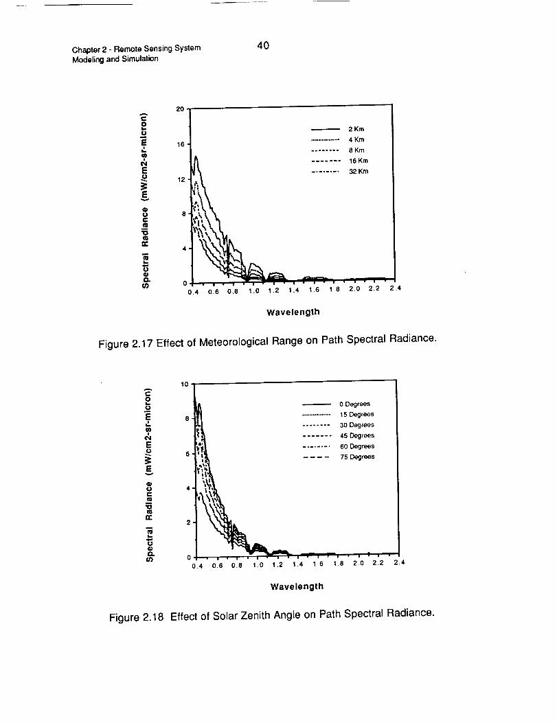
Chapter 2 - Remote Sensing System
Modeling and Simulation
40
f..
oum
E
?
E
Ev
ool=
1o
¢
m
PgoQ.
2O
12
2 Km
............. 4 Km
........ 8 Km
....... 16 Km
32 Km
0 , • . - = '• • | |
0.4 0_6 0.8 1.0 1.2 'l.4 1.6 1.8
Wavelength
Figure 2.17 Effect of Meteorological Range on Path Spectral Radiance.
_ 0 Degrees
i 8-_ ................ is o,_,ees_;_t ........ 30 Degrees
t(_ ....... 45 Degrees
6 J_l_ ........ 60 Degreos
E ItS,_ .... 75_rees
0.4 0.6 0.8 1.0 1.2 1.4 1.6 1.8 2.0 2.2 2.4
Wavelength
Figure 2.18 Effect of Solar Zenith Angle on Path Spectral Radiance.

41Chapter 2 - Remote Sensing System
Modeling and Simulation
12
" 10 .,_ 60 DegreesU
_t_' _ ........ 30 Degrees
' i0.4 0.6 0.8 1,0 1.2 1.4 1.6 1.8 2.0 2.2 2.4
Wavelength
Figure 2.19 Effect of Sensor Zenith Angle on Path Spectral Radiance.
24A
c
ouE 20L
?
E 16
Ev 12
@t,.)e.,.¢=
on
ffl
Albedo- 100
............... Albedo-0.10
........ Albedo=0.01
0 • I • I r_ _ |m ,
• ,,: ,: .......0.4 0,6 0,8 1,0 12 14 1.6 1.8 2.0 2,2 2.4
Wavelength
Figure 2.20 Effect of Surface Albedo on Path Spectral Radiance.

Chapter 2 - Remote Sensing System 42
Modeling and Simulation
These curves give an indication how the components of the atmospheric
model vary under different conditions. In general, they show how a hazier
atmosphere will allow less radiance to be received by the sensor from the
surface, yet increases the path radiance, and how the angle of illumination or
view can decrease the signal radiance as well as increase the path radiance.
The path radiance is also seen to increase with surface albedo.
An experiment was performed to test the suitability of the atmospheric
model by comparing the radiance received by a satellite to that simulated by the
model from a description of the scene conditions and the reflectance of the
surface. A test site in Hand County, South Dakota was chosen from data
gathered as part of the LACIE program (Hixson, et al., 1978). On July 26, 1978,
reflectance data was gathered at approximately the same time as the Landsat 2
MSS passed over the area. The parameters of these sensors are shown in
Table 2.7.
Table 2.7 Data Set for Hand County, South Dakota, July 26,1978.
Landsat 2 Multispectral Scanner
Spectral ChannelsSceneAltitudeGround Size of IFOVTime
4 bands, 0.4 - 1.1 _m21281-16232918 Km80 Meters1623 GMT
Helicopter Field Spectrometer System
Spectral ChannelsAltitudeGround Size of FOVTime
60 bands, 0.4 - 2.4 I_m60 Meters25 Meters1505- 1601 GMT
A particular area having four large nearly square fields was selected for
test. Table 2.8 contains the field numbers from the LACIE experiment and the
crop types.

43 Chapter 2 - Remote Sensing SystemModeling and Simulation
Table 2.8 Description of Test Fields.
Field Number|l
Field 290Field 168Field 289Field 288
Crop TypeSpring Wheat
Millet
Spring WheatMillet
Ground Cover
30 Percent10 Percent30 Percent90 Percent
In order to compute the radiances received by the MSS, a table of
conversion constants was obtained from the work by Richardson, et al., (1980).
Table 2.9 shows the A i and Bi used to compute from the digital counts DC i the
radiance present at the input of Landsat 2 MSS in band i. Equation 2.21 shows
how these constants are used to compute the radiance. The units of A are
mW/(cm2-sr-digital count) and for B are mW/(cm2-sr).
Table 2.9 Conversion Constants Between Radiance and Digital Counts.
Band1234
A0.02010.01340.01i50.0603
B0.080.060.060.11
L. = A. DC. + B. (2.21)I I I I
In generating the simulated radiance, the atmospheric model described
earlier in this chapter was used with the radiances integrated over the nominal
wavelength intervals of each band of the MSS sensor. Thus, the radiance in
each band i was generated as in equation 2.22.
I 1 0 1 01 Ri + Li,Pat h . Li,Pat h Ri + Li, PathL i = _- Ei,Tota I Ti,Atm (2.22)

Chapter 2 - Remote Sensing System
Modeling and Simulation
44
Here, R i is the average reflectance in band i. Table 2.10 gives the
atmospheric and goniometric conditions present at the time of observations.
Table 2.10 Scene Conditions at Time of Observations.
i Meteorological Range (V_)
Solar Zenith Angle (0solar)
Solar Azimuth Angle (¢solar)
Diffuse Irradianc e Constant (KD)
31 Km
39 o
119 o1.26
i
Table 2.11 contains the LOWTRAN settings used in generating the
simulated atmospheric effects.
Table 2.11 LOWTRAN Settings for Experiment.
IAtmospheric ModelAtmospheric HazeAtmospheric ScatteringAerosol Phase FunctionsAerosol Profile
it
1976 U. S. StandardRural Extinction
MultipleMie-generated
Back_lround Stratospheric
All other LOWTRAN parameters were set to zero, or the default. Table
2.12 shows the atmospheric components generated by LOWTRAN for each of
the spectral bands, while Table 2.13 compares the simulated to the actual
radiances received by the satellite.

45 Chapter 2 - Remote Sensing SystemModeling and Simulation
Table 2.12 Atmospheric Components for the Hand County Test Site.
Band
1234
ETotal/c--_- /
16.29614.03610.843
19.329 ,
Tatm
0.6840.7460.7640.774
mW!
"Path. 1, c
1.1310.7350.4340.524
Lpath,OI_ 1
0.2480.1280.0680.071
Table 2.13 Comparison of Actual and Simulated Radiances (in mW/(cm2-sr)) forTest Site in Hand County, SD.
Field 290Band 1Band 2Band 3Band 4
Field 168Band 1Band 2Band 3Band 4
Field 289Band 1Band 2Band 3Band 4
Field 288Band 1Band 2Band 3Band 4
FSSReflectanc_
0.0630.O830.1660.240
O.068O.O880.1210.182
O.O58O.0780.1430.208
O.0430.0310.2520.388
MSS AverageDigital Count
21.526.944.220.7
23.731.036.816.6
22.127.643.220.1
LandsatRadiance
0.5120.4210.5681.358
0.5560.4750.4831.111
0.5240.4300.5571.322
SimulatedRadiance
O.5270.4550.5661.323
0.5490.4750.4311.020
0.5050.4350.4971.156
PercentError
+2.9+8.1-0.4-2.6
-1.30.0
-10.8-8.2
18.314.866.136.6
0.4480.2580.8202.317
0.4390.250O.8252.094
-3.6+1.2
-10.8-12.6
-2.0-3.1+0.6-9.6
A scatter plot of the simulated radiances versus the measured ones is
shown in Figure 2.21. The solid line is a best linear fit to the points with a
regression coefficient of 0.99, while the dashed line represents the ideal of
equal radiances.
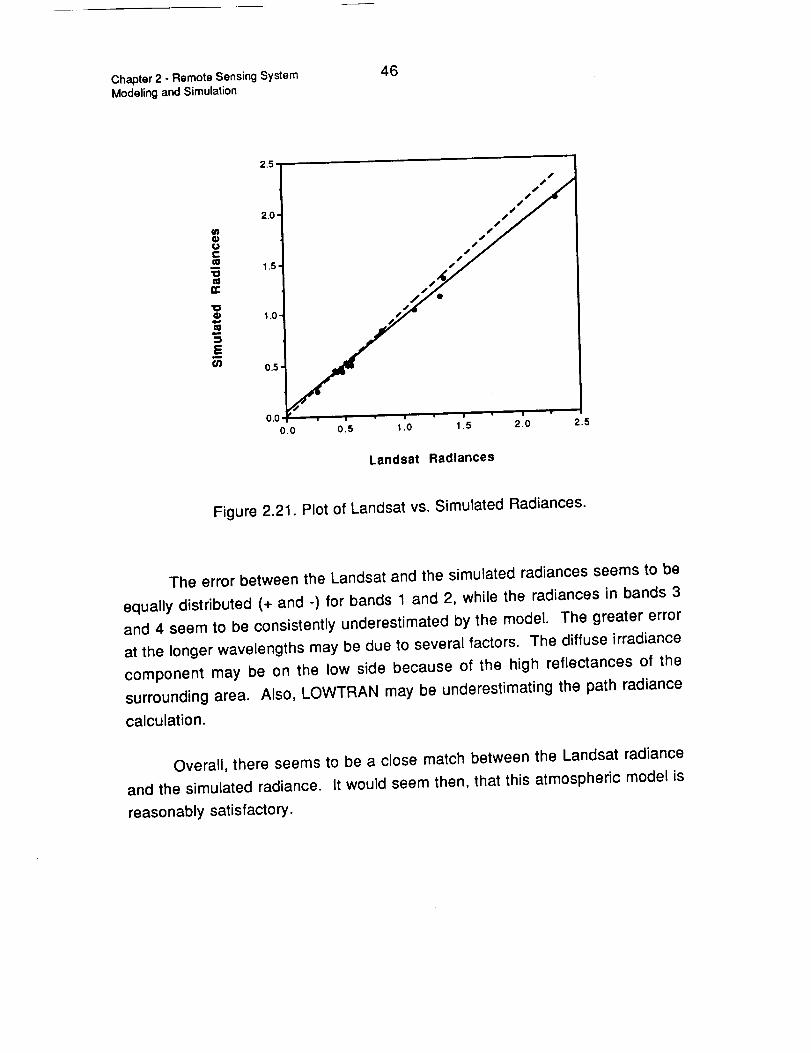
Chapter 2 - Remote Sensing System
Modeling and Simulation
46
2.5
2,0 '
oc
¢1 1.5
"oQ 1.0
¢1
E_ 0.5
0.0
0.0
s
ts_Ss_4s SSSSSSSSSSS
* 'w
i ' '0 5 1 0 1.5 2.0 2.5
Landsat Radiances
Figure 2.21. Plot of Landsat vs. Simulated Radiances.
The error between the Landsat and the simulated radiances seems to be
equally distributed (+ and -) for bands 1 and 2, while the radiances in bands 3
and 4 seem to be consistently underestimated by the model. The greater error
at the longer wavelengths may be due to several factors. The diffuse irradiance
component may be on the low side because of the high reflectances of the
surrounding area. Also, LOWTRAN may be underestimating the path radiance
calculation.
Overall, there seems to be a close match between the Landsat radiance
and the simulated radiance. It would seem then, that this atmospheric model is
reasonably satisfactory.

47 Chapter 2 - Remote Sensing System
Modeling and Simulation
2.3 Sensor Modeling
The sensor portion of optical remote sensing systems performs the task
of sampling the continuous spectral radiance of the scene in the spectral,
spatial, radiometric, and temporal domains. This results in a digital
multispectral image of a scene at a certain moment in time, with a discrete
number for the radiance at each spot in the scene and for each spectral region.
The modeling of imaging sensors can be quite complex indeed. One
may consider the propagation of the optical waves through the sensor optics
(including aberrations), the conversion from light to electrons in the detector
material, and the effects in the signal conditioning electronics. Goodman (1968)
provides a good discussion of the propagation of optical waves in imaging
systems from a linear systems point of view. Texts by Hudson (1969), Pinson
(1985), and Wyatt (1987), and chapter eight of Colwell (1983) cover the entire
detection process from the optical system through the detector electronics.
In this research, the modeling of sensors is approached from a lumped
systems perspective. Figure 2.22 shows a block diagram of the major
components of a multispectral sensor.
SPATIAL
RESPONSE
SPECTRAL
RESPONSE
ELECTRICAL
NOISE
A/D
CONVERSION
Figure 2.22 Sensor System Components.

Chapter 2 - Remote Sensing System 48Modeling and Simulation
The scene is sampled spatially by its being imaged onto a detector array
that is either scanned sequentially down the scene, or consists of a focal plane
array that gathers the two-dimensional image in a small but finite time interval.
These sampled pixels are also dispersed onto separate detectors for each
spectral band to the perform the spectral sampling.
The signals from these detectors are then amplified (electrical noise
effects occur here) and calibrated before being quantized into discrete values.
The model shown here is very general and could be enhanced to include
very detailed effects such as the aberrations in the optical propagation in the
optical system, spatial misalignment of the detectors, or electrical bandwidth of
the amplifiers. But in this report, the model will be relatively simple within this
generality. The model will be limited to a simple point spread function for the
spatial response, a simple multiplication of the sensor response for the spectral
response, and a noise model containing electrical noise, calibration error, and
quantization effects.
In the following subsections 2.3.1 and 2.3.2, models are presented for the
sampling and noise processes. In subsection 2.3.3, a detailed model is
presented for a future remote sensing imaging spectrometer. Appendix D
contains complete descriptions of several multispectral scanners. In subsection
2.3.4, the computation of radiometric performance measures is discussed.
2.3.1 Sampling Effects
In the creation of the digital image the continuous spectral radiance of the
scene is sampled spatially, spectrally, and radiometrically (ie., A/D conversion).
The following paragraphs describe these forms of sampling.
1. S.Datial Sampling. The optical Point Spread Function (PSF) is the two-
dimensional analog of the system impulse response in linear system theory
(Goodman, 1968). It is the response of the optical system to an infinitely bright
point source, usually represented by the Dirac delta function 5(x,y).

49 Chapter 2 ° Remote Sensing SystemModeling and Simulation
In the simulation model, no parametric form for the PSF is assumed.
Rather, a table of values derived from measurements of the real devices is used
to define the PSF. Thus, this form includes many of the aberrations present in
the instrument optics.
The discrete representation of the response of the optical system is given
by equation 2.23. The PSF h(u,v) is represented as the product of separable
line spread functions hx(- ), and hy(.), across the two spatial dimensions. The
response is normalized to unit area by dividing by the area under it.
h(u,v) = (A x gx)(Ay gy) hx(O)hy(p ) 8(u- gx, v- gy) (2.23)o-1 p=l
Where,
(u,v) - spatial domain locations (meters)
A x - sum of across scene line spread function coefficients
Ay - sum of down scene line spread function coefficients
gx = _UH - ground interval between hx coefficients (meters)
gy = _VH - ground interval between hy coefficients (meters)
AU - angular distance between hx coefficients (radians)
AV - angular distance between hy coefficients (radians)
H - height of sensor (meters).
Also, O+1 and P+I represent the number of coefficients in the across
scan and down track line spread functions, respectively, and hx(P/2 ) and
hy(O/2) contain the maximum response.
Equation 2.23 gives the response for a vertical viewing sensor. For
sensor zenith angles > 0°, the distance on the ground between the coefficients
must be rotated by the azimuthal angle _vi_w, and scaled by the zenith angle
(}view. This is shown in equation 2.24.

Chapter 2 - Remote Sensing System 50
Modeling and Simulation
E0 I=icos0vew)sn0vow)Tigygx1gy - sin(_view ) coS(_view)_J cOS_view)
(2.24)
In applying this spatial response to the scene spectral radiance function
derived in section 2.2.3, equation 2.25 is used. This equation is repeated for all
image pixel locations (i,j) and scene wavelengths m.
GxGy o+1 P+l _iS x - og x jSy- pgy /;)EE' . ooo ' .m0=1 p=l
(2.25)
Sx and Sy are the across scene and down track sampling intervals for the
image pixels. In the case of off-nadir viewing these also must be scaled and
rotated as the ground coefficient intervals were in equation 2.24. Note that
since the scene radiance array has discrete pixel locations all index quotients
are rounded to the nearest integer. Also, at the edges, the extreme row or
column is repeated as necessary to allow for the complete application of the
spatial response.
The PSF is often approximated by a truncated Gaussian curve.
Measured PSF's often are nonsymmetrical and can iaclude ringing at the tails
of the response; thus the Gaussian shape does not truly represent the actual
PSF. Although in some cases, it can be close enough to justify its use in
theoretical modeling.
2. Spectral Sampling. The spectral response of a multispectral sensor
consists of the continuous response of each channel to the spectral radiance
received by the sensor. In the simulation, the application of the discrete
response to the incoming spectral radiance Lx,sensor(i,j,m ) is as shown in
equation 2.26.

51 Chapter 2 - Remote Sensing System
Modeling and Simulation
Msl(m)
Llmag e (i,j,I) = z_._, k_.,Senso r (i,j,m) N(I)m=l
(2.26)
Where,
,_._ - scene wavelength increment in l_m
sl(m) - normalized response of band I to spectral wavelength m
Limage(i,j,I ) - radiance received by band l at pixel location (i,j)
Lx, sensor(i,j,m ) -incoming spectral radiance from pixel location (i,j)
at wavelength m
N(I) - normalizing factor for nominal bandwidth variations.
The normalizing factor N(I) is the ratio between the actual bandwidth as
measured by the area under the normalized response curve and the nominal
bandwidth of the channel. This factor is often necessary to match the published
gain setting between the real instrument and a modeled version. Price (1987)
discusses calibration problems of this sort and presents tables of the actual
bandwidth for several multispectral scanners.
For the imaging spectrometers modeled in this report, the spectral
resolution of the sensor is the same as the scene. Thus, for these sensors there
is only one term present in equation 2.26.
3. Radiometric SamDling. After the continuous spectral radiance across
the scene has been sampled spectrally, and spatially, and the noise (discussed
in the following subsection) has been added in, the received value is converted
to a discrete level by equation 2.27.
• (2e-1)} (2.27)
Here, Q is the number of radiometric bits of the sensor, and LFulI,I is the
published full scale equivalent radiance for sensor band I. This introduces

Chapter 2 - Remote Sensing SystemModeling and Simulation
52
quantization noise uniformly distributed with an equivalent radiance variance
shown in equation 2.28 for each sensor band.
(2.28)
2.3.2 Electrical Noise Modeling
Malaret (1982) performed a study of the general noise effects in
multispectral sensor systems and their impact on data analysis. In this
research, his model for the electrical noise present in these types of sensors will
be used, augmented by models for radiometric and calibration errors. Figure
2.23 contains a block diagram of this noise model showing the signal
dependent shot noise, thermal noise, radiometric error, and calibration error.
IncomingRadiance
AbsouteI Re'at'veRadiometric _ Shot I Thermal Calibration
Error Noise I Noise Error
=_ _j__ _ D_tectorOutput
Figure 2.23 Noise Model of Sensor.
In his work, Malaret showed how the shot noise in a multispectral sensor
can be modeled as a zero mean Gaussian process with its variance
proportional to the signal level (assuming the typical signal levels associated
with Landsat sensors.) In this research, the shot noise signal dependence is
implemented by having the variance of a Gaussian random number generator
proportional to the signal level. These random numbers are then added to the
signal level.

53 Chapter 2 - Remote Sensing SystemModeling and Simulation
Thermal noise has been shown to have a Gaussian distribution also with
zero mean and a variance proportional to the product of detector temperature,
bandwidth, and resistance. These factors are assumed to be relatively
constant, and thus the level of the thermal noise is fixed. It is implemented as a
Gaussianly distributed random number added in to the signal level received by
the sensor.
Two types of radiometric error are found in the sensor system, absolute
and relative calibration error. Absolute errors imply a deterministic change in
output level, while relative errors are manifested as stochastic noise. Table
2.14 shows several causes for these errors and the type of error produced.
Table 2.14 Sources and Types of Radiometric Errors.
Error Source
Change in transmittance of opticsChange in gain of detector amplifiersChange in characteristics of calibration standardChange in detector quantum efficiency
Error Typeabsoluteabsoluteabsoluterelative
Absolute errors are introduced in the model through additive offset. The
level of error is constant across the detectors, but is signal and wavelength
dependent. The model for the relative calibration error has been developed
under the assumption that each detector channel in the imaging array may
undergo a random and independent change in its response over time. Thus,
the radiance level required for a given output may differ from detector to
detector.
From the statistics given in Castle, et al. (1984) it was determined that the
actual output of detectors may vary as much as 1% from the calibrated output
given the same input. Assuming an uniform distribution for this error, then the
multiplier for the uniform random number generator would be chosen to be ±1%
of the signal level. The standard deviation of this error is given in equation 2.29.

Chapter 2 - Remote Sensing System 54Modeling and Simulation
2 * 0.01 {signal level}acal- _ (2.29)
Depending on the spatial arrangement of the detectors, the relative
calibration error may be constant in one spatial direction. For example, a linear
array of detectors may cause relative errors across the image, but since the rest
of the image is formed by the motion of the sensor platform, the relative error is
constant down the columns of the image. This may cause a vertical striping
effect. Or, for a line scanning detector array, the striping may be horizontal as
was found in early Landsat MSS sensors. Thus, in implementing the calibration
error model, the type and arrangement of detectors must be considered.
2.3.3 HIRIS Model
In this subsection, a model for the High Resolution Imaging Spectrometer
(HIRIS) is presented. The instrument is described in Goetz and Herring (1989).
HIRIS is meant to be used in an on-demand mode of operation, gathering data
at the request of a science investigator. Kerekes and Landgrebe (1989a)
present a full description of this instrument and its performance. Table 2.15
contains a brief overview of the instrument and its general design parameters.
Table 2.15 HIRIS Functional Parameters.
Design AltitudeGround IFOVSwath Width
Spectral Coverage
Average Spectral Sample Interval
0.4 - 1.0 _m
1.0 - 2.5 _mPointing
Down-track
Cross-track
Data EncodingMaximum Internal Data Rate
Maximum Output Data RateImage Motion Compensation Gain
705 Km30 m20 Km
0.4 - 2.5 I_m192 Bands
9.4 nm
11.7 nm
+60o/-30 °
+20o/-20 °
12 bits/pixel512 MBPS300 MBPS
1,2, 4, or8

55 Chapter 2 - Remote Sensing SystemModeling and Simulation
For this research the model shown in Figure 2.24 is used for the HIRIS
instrument. This model version has 201 equally spaced (10 nm intervals)
spectral bands from 0.4 to 2.4 _m and includes most major spectral, spatial, and
radiometric effects of the instrument.
OPTICS
Incoming |
Spectral
Radiance /
OpticsTransmission
J Spatial
7 Focusing
DETECTOR
Detector Shot
Response Noise
Dark
Current
I ReadNoise
SIGNAL CONDITIONING
Lt' I(_ Signal [..__ RelativeScaling CalibrationError
A/DConversion
OutputDigitalNumber
Figure 2.24 HIRIS Model Block Diagram.

Chapter 2 - Remote Sensing System 56
Modeling and Simulation
Instrument parameters have been obtained from a progress report by
JPL (1987). These parameter levels are based upon preliminary specifications
and prototype testing. The following paragraphs and figures detail the blocks in
the overall diagram and present relevant parameter values.
The sensor has two detector arrays to cover the entire spectral response.
The Very Near Infrared (VNIR) array covers 0.4 - 1.0 p.m, while the Short Wave
Infrared (SWIR) array covers 1.0 - 2.5 _m. The scene is imaged line by line as
the sensor passes over. Each scene line is sampled spectrally by being
dispersed across the detector arrays.
The spectral transmittance of the instrument optics is shown in Figure
2.25. Note the low response at the spectral gap between the VNIR and the
SWIR arrays at 1.0 i_m.
O
E
¢-
I-
a.¢D
0.3'
0.2 ¸
0._'
/------.
• I 1' '| • I • a • I • I • I
0.6 0.8 1.0 1.2 1.4 1.6 1.8
0.0 • | • ! ' •
0.4 2.0 2.2 2.4
Wavelength (micrometers)
Figure 2.25 Spectral Transmittance of Optics.
The normalized spatial response of the optics and field stop is assumed
to be similar to the that of the Landsat Thematic Mapper instrument, as they both

57 Chapter 2 - Remote Sensing System
Modeling and Simulation
have a Ground Instantaneous Field of View (GIFOV) of 30 meters. Figure 2.26
shows the measured down scene and across scene normalized responses as a
function of angular distance for the TM, taken from Markham (1985). The data
points shown are the discrete values used in the simulation. At the nominal
altitude of the HIRIS instrument, the distance on the ground between these
points is approximately seven meters.
1.2
1.0-
0.8'C00,.
0 0.6'
1D0.4'
N
0.2-0Z ,
0.0"
-0.2
-8 • ' | • i • | • i • ! • i0 • i-60 -40 -20 0 20 4 60
Angular Distance (rnlcroradlans)
Figure 2.26
8O
Normalized Spatial Response.
------=---- Across Scene
....... ,e ...... Down Scene
The radiometric conversion from the incoming spectral radiance
(mW/cm2-sr-i_m) is accomplished by dividing by 1000 mW/W, multiplying by the
transmittance of the optics and by the A_ (the product of the detector area and
the solid angle of view) of the optics. The output of the optics model P_., the
incident spectral power, is then in units of watts/#m. The A£ used in the model
is 1.44 x 10 .6 cm2-sr.
The spectral quantum efficiency q of the detectors is shown in Figure
2.27. The incident spectral power P_. at wavelength X is converted to a number
of electrons S at the detector by the integration of the incident photon level over

Chapter 2 - Remote Sensing SystemModeling and Simulation
5B
the pixel integration time. Thus, the overall radiometric conversion is shown in
equation (2.30).
S = L_.,Scene * 1000 mW • A_ * T • A_. • 11* _ • t (2.30)1 W optics
Where,
A_. = 0.01 p.m, wavelength interval of spectral samples
;L = wavelength of interest (_m)
h = 6.62 x 10 -34 Joule-sec, Planck's constant
c = 3 x 10⁸ meters/sec, the speed of light
t = 0.0045 seconds, pixel integration time
q = detector quantum efficiency.
Since the noise level data and full scale specifications were obtained in
terms of number of electrons, the signal level is stated in these same terms and
is unitless.
UC
,.i.=
UJ
E
"!Cl
1.0 o
0.9-
0.8
0,7
0.6-
0.5-
0.4-
0.3-
0.2-
0.1
0.0 • i • i . ! • i . ! . i . i . i . ! |
0.4 0.6 0.8 1.0 1.2 1.4 1.6 1.8 2.0 2.2 2.4
Wavelength (micrometers)
Figure 2.27 Spectral Quantum Efficiency.

59 Chapter 2 - Remote Sensing SystemModeling and Simulation
The Image Motion Compensation (IMC) is implemented through
movement of the down-track pointing mirror to offset the platform speed and
effectively multiply the pixel integration time by the gain state selected: 2, 4, or 8.
The noise in this model consists of a deterministic dark signal level and
absolute radiometric error, and random shot noise, read noise, and relative
calibration error. Thermal noise has been found to be insignificant. All noise is
considered to be stochasticly independent between noise types and spectral
bands. Table 2.16 contains several parameters of the detector arrays.
Table 2.16 Parameters of Detector Arrays in Terms of Electrons (e-).
Dark CurrentRead Noise Standard DeviationFull Scale Level
VNIR SVVlR0 e- 27000 e-
300 e- 1000 e
577,395 e- 1,441,440 e-
The dark current is simply added to the received signal level in the
model. The absolute radiometric error is included in the detector portion of the
model by multiplying the total signal by (1 + ER), where ER is the decimal level of
error. Read noise is added in as a zero mean Gaussian random number with a
standard deviation as in Table 2.16. Within each detector array, the read noise
level is assumed to be constant over wavelength.
The shot noise in the model consists of zero mean Gaussian random
numbers with a standard deviation equal to a function of the total signal level in
the detectors. This total signal is comprised of the incoming radiance, and the
dark current level mentioned above. Figure 2.28 shows several points relating
total signal and shot noise levels taken from the JPL report, along with a curve
showing the square root of the total signal. It can be seen that the shot noise
level is almost exactly the square root of the total signal level.
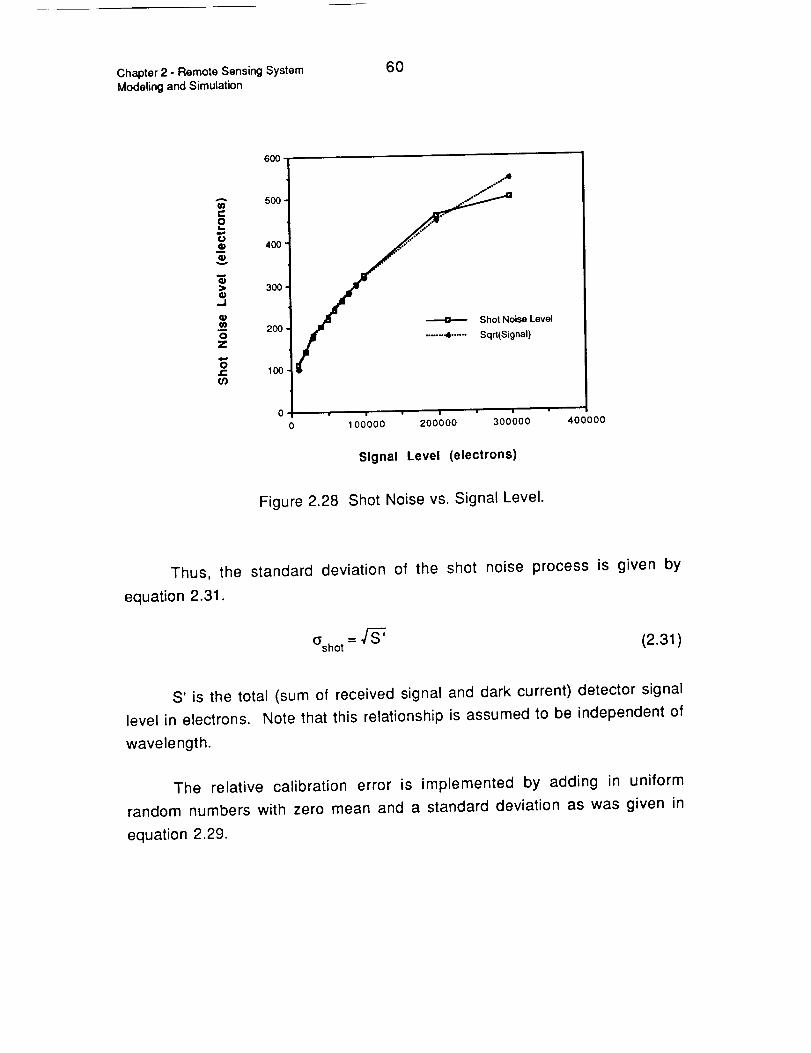
Chapter 2 - Remote Sensing System
Modeling and Simulation
60
600
"" 500.U)
oo
400'
> 300'0
,,J
-_ 2oo.o
Z
0e- 100.
if)
ise Level
...... • ...... Sqrl(Signal)
' ' o100000 200000 300 O0
Signal Level (electrons)
40O000
Figure 2.28 Shot Noise vs. Signal Level.
Thus, the standard deviation of the shot noise process is given by
equation 2.31.
(_shot= "/_ (2.31)
S' is the total (sum of received signal and dark current) detector signal
level in electrons. Note that this relationship is assumed to be independent of
wavelength.
The relative calibration error is implemented by adding in uniform
random numbers with zero mean and a standard deviation as was given in
equation 2.29.

61 Chapter 2 - Remote Sensing SystemModeling and Simulation
The conversion from the e-levels S" (received signal plus noise and
calibration error) to a digital number (DN) occurs as in equation 2.32.
where,
,Is' l /1DN - nin IMC oF • 2Q" 1 (2.32)
IMC = IMC Gain State
F = Full Scale Electron Level (shown in Table 2.16)
Q = Number of radiometric bits (nominally 12)
The division by the IMC gain state is included to preserve the dynamic
range of the detectors over the various gain states.
2.3.4 Radiometric Performance Measures
Several measures of the radiometric performance of remote sensing
instruments are commonly used. All of these measures are a function of
wavelength, atmospheric conditions, sensor response, and sensor electrical
noise. In this subsection, two common ones are described and defined as they
are used in this research.
Noise Equivalent change in Reflectance (NEAp) is used in identifying the
smallest differences in the surface reflectance that are detectable by the sensor.
It is defined as being the equivalent change in the reflectance of the surface to
match the total noise level in the sensor. In terms of the parameters used in this
report, this is given in equation 2.33. Note that these parameters are dependent
upon the sensor spectral band for which the calculation is being made.
_shot + O_therm + O_read + _quant + 02_1
NEAp = 1 (2.33)_- Ex,Tota I T_.,AtmB(;L)
B(_.) is the conversion from incident spectral radiance to the signal level
in the detector for the appropriate band. For general multispectral scanners,

Chapter 2 - Remote Sensing Syster_" 62Modeling and Simulation
this is the summation given in equation 2.26, while for the HIRIS model it is the
right side of equation 2.30. ine resulting signal level is then scaled by the
absolute radiometric error (1 +ER).
The Signal-to-Noise Ratio (SNR) is another common measure of
performance of a remote sensing instrument. It is commonly expressed as the
log of the ratio of the signal level of interest to the total noise level.
In many Earth resource analysis remote sensing applications, the output
product is some form of classification map of the observed area. The
classification is usually obtained by a computer algorithm that uses the mean
and covariances of the multispectral image data to distinguish between the
classes. Thus, in this application not only are signal levels important, but so are
signal power variations.
In this report, two types of SNR are defined. One based on the mean
signal level, while the other is based on the covariance of the received signal.
The voltage SNR is useful for determining the dynamic range required of the
sensor, white the power SNR is useful for studying the sensitivity of the sensor
in discriminating among surface class types.
The voltage SNR is defined for a sensor band by dividing the mean
signal level in that band by the square root of the sum of the noise levels for that
band, as in equation 2.34.
Voltage SNR = 20 IOglo { %/O__shot
_- Ex,TotaiTAtrn _ B(k)
+O_therm +O_re_ d +O2qquant+l_cal
(2.34)
Here, _ is the mean reflectance of the surface, and B(;L) is defined as
above. The power SNR is defined for one wavelength m in the HIRIS model to
be as in equation 2.35.

Power SNR = 10 Ioglo f
63 Chapter 2 - Remote Sensing System
Modeling and Simulation
(2.35)
Here, o2m is the variance of the surface reflectance for wavelength m. In
calculating the SNR for a particular scene, the mean and variance of the surface
reflectance are usually calculated from the combined data set of all classes
represented in the scene.
In computing the power SNR for the multispectral scanners, or for
features derived from the HIRIS sensor by combining bands, the signal levels
cannot be simply added because of the band-to-band correlation present in the
reflectance data. In these cases, the signal variance is the sum of the individual
variances, plus terms due to the covariance between each pair of wavelengths
m and n, combined in the feature as in equation 2.36.
Combined Power SNR = 10 log10 I M L M E
="<,,.--r,>m=l n-1
O'_shot + O_therm + O_read + _quant +O2_12.36)
M L is the number of wavelengths combined for the band or feature, while
B+(_.) is the product of the radiance received from a completely reflecting
surface and the conversion to the signal level in the sensor for the appropriate
wavelength. The m,n entry in the reflectance spectral covariance matrix is
denoted here as O'mn. Also, the noise variances as used here are the sum of the
individual wavelength variances combined appropriately.
2.4. Processing
Processing plays the most important role in remote sensing systems as it
is the part that provides the information that the system is designed to acquire.
Aspects of processing in remote sensing are discussed in chapters 17 through

Chapter 2 - Remote Sensing bys_em 64Modeling and Simulation
24 of Colwell (1983), chapters three through six of Swain and Davis (1978), and
in the text by Richards (1986). Nunlerous other texts and articles have been
published dealing with the processing of remotely sensed images.
Table 2.17 shows a list of typical functions used in the processing of
remotely sensed images. The task of the processing portion of the system is to
take the multispectral image from the sensor, and any other input data or
algorithms, and then compute an output information product. This product may
be a classification map showing to which of the informational classes each pixel
belongs, or it may be a summary of the total area within the image that belongs
to each of the classes. The processing functions shown in Table 2.17 aid in
this task by allowing the information to be obtained efficiently and accurately.
Table 2.17 Example Processing Functions.
Proc?ssing Typ?
Radiometric
G'eornetric
Data Reduction
Class Separability
Classification
Example
Calibration
ScalingCompression/
Decompression ,,,RegistrationResamplincjFeature Extraction
Feature CompressionTraining Field SelectionInterclass DistanceIntractass Distance
Unsupervised (Clustering)SupervisedClass Area Measures
In the rest of this section these processing functions are discussed, and
where appropriate, models are presented for use in the simulation of remote
sensing systems.

65 Chapter 2 - Remote Sensing SystemModeling and Simulation
2.4.1 Radiometric Processing
The goal of radiometric processing is to allow accurate and repeatable
calibration of the radiance levels represented by the digital numbers in the
multispectral image. This is important when comparing images over the same
area from different dates or sensors. Price (1987) discusses the accurate
calibration of several sensors for comparative purposes. Papers by Fischel
(1984), Murphy, et al., (1984), and Castle, et al., (1984) discuss the calibration
of the Landsat Thematic Mapper sensor.
For modeling purposes, the calibration models presented in section 2.3.2
are useful in studying the effect of these radiometric errors.
2.4.2 Geometric Processing
Geometric processing is generally concerned with correcting spatial
distortions in the multispectral image due to scanning variations, detector
misalignment, or view angle effects. The aim of such processing is again to
allow comparison of images, or to match images to other forms of spatial data
such as topographical or land use maps.
Spatial distortions are often corrected by developing a mapping function
from the image to the control map by using identifiable features (control points)
in the scene. Pixels in between these points are often resampled to give a
desired spatial resolution. The papers by Park, et al., (1982 and 1984), and
Schowengerdt, et al., (1984) discuss the effects of these corrections.
Another form of geometric distortion is known as misregistration, and is
due to the effective misalignment of detectors of the various spectral bands.
This may occur due to distortion in the imaging optics, or to the physical location
of the detectors. It effectively causes the pixels of different bands to be imaged
from a slightly different part of the scene. Misregistration has been studied by
Cicone, et al., (1976), Billingsley (1982), and Swain, et al., (1982). In the study
by Swain, et al., it was found that misregistration by as little as 0.3 pixels can
affect classification accuracy.

Chapter 2 - Remote Sensing Syslem 66Modeling and Simulatioq
Although they would be relatively straightforward to implement in the
sensor spatial model, these forms of geometric distortion were not studied in
this research.
2.4.3 Data Reduction
in most cases it is either necessary, or at least advantageous, to reduce
the amount of data in a muttispectral image without diminishing the
informational content. In the case of the upcoming HIRIS instrument the normal
operating mode produces data at a rate exceeding the capabilities of the
satellite's communication channel, thus necessitating some form of on-board
editing. For lower dimensional sensors such as Landsat TM or aircraft
scanners, it has been shown that under conditions of limited training samples,
cJassificatJon accuracy decreases as more spectral bands are usecl in the
classification (see Hughes, 1968, and Chandrasekaran, 1975.)
This data reduction may be accomplished spatially, spectrally, or by
reducing the radiometric resolution of the data. The spatial reduction may be as
simple as deleting every other pixel or reducing the swath width of the sensor,
or as complex as a scheme described in Ghassemian (1988) which retains
much of the spatial detail in the image while reducing the data to a set of
features. Reducing the radiometric resolution may be used and usually will not
increase the noise level significantly, unless the quantization error becomes the
dominant source of noise in the image.
Spectral reduction through the Karhunen-Loeve (or principal component)
transformation was studied in Ready and Wintz (1974). This method has proved
to be useful in reducing dimensionality while retaining class separability, even
in cases of limited training samples (Kalayeh, et al., 1983, and Muasher and
Landgrebe, 1983). However, it requires computation of the eigenstructure of
the covariance matrix and thus is not easily implemented at high data rates.
With the advent of imaging spectrometers such as HIRIS, on-board
feature selection algorithms that can be implemented through simple
programmable operations, such as summations, have been studied. Chen and
Landgrebe (1988) have extended a method first proposed by Wiersma and

67 Chapter 2 - Remote Sensing System
Modeling and Simulation
Landgrebe (1980) to select spectral regions to be combined. The algorithm
uses training samples from similar data, or ground reflectance, and selects
wavelengths to be combined based upon the eigenfunctions of the spectral
covariance matrix. A simple set of summation coefficients may then be
transmitted to the satellite and used to reduce the data rate. Factors of data
reduction of 10 or more have been found to be possible with little loss in the
class recognition accuracy (Chen, 1988).
In the simulation program developed in this report, data reduction may be
accomplished for the HIRIS model through the combination or weighted
summation of spectral bands.
2.4.4 Class Separability Measures
Class separability measures are computed from the statistics of known
class samples, and are used to obtain an idea of the statistical distance
between informational classes. These measures have been studied both as a
feature selection technique (Swain and King, 1973), as well as an estimate of
error probability (Kailath, 1967, and Whitsitt and Landgrebe, 1977.)
Many of these separability measures are for two classes, and are
computed from the mean vectors and covariance matrices. As an example, the
Bhattacharyya distance Bkl is given in equation 2.37 between class k and class
I with mean vectors Z--k and _ , and covariance matrices _k and _l.
21,0ge|_l__2= (2.37)
Multiclass separability measures can be obtained from apriori class
probability weighted pairwise summations of such two class separability
measures. Whitsitt and Landgrebe (1977) discuss this and other ways of
measuring multiclass separability.

Chapter 2 - Remote Sensing SystemModeling and Simu!aticn
68
Fukanaga (1972) also presents a multiclass separability measure that is
used in canonical analysis to reduce the dimensionality of data through a linear
transformation (Merembeck and Turner, 1980). This measure JF is described
by equation 2.38.
where,
-1
JF = tr SwS b (2.38)
K
S w = _ Pk_k
k=l
K
S b= _ Pk(Zk "z o) (Z k
k=lK
2;=T_.,z,k=l
- Zo) T
In these equations, Pk is the apriori probability of class k, and the mean
vectors and covariance matrices are noted above.
In the simulation program, both a pairwise summation of the
Bhattacharyya distance and the Fukanaga multiclass measure are
implemented. The class statistics are computed from designated areas within
the known class areas.
2.4.5 Classification Algorithms
The classification of a multispectral image into informational classes may
be done in an unsupervised manner by a computer algorithm, or in a
supervised approach by an analyst working interactively with the computer. In
either case, the accuracy of such a classification can then be computed by
comparing the resulting class map to a known class map of the area.
Classification accuracy has also been estimated from the class statistics.
Fukanaga and Krile (1969) present an analytical method for estimating
accuracy in the two class Gaussian case, while Whitsitt and Landgrebe (1977)
discuss several considerations in multiclass error estimation.
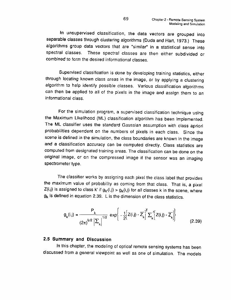
69 Chapter 2 - Remote Sensing SystemModeling and Simulation
In unsupervised classification, the data vectors are grouped into
separable classes through clustering algorithms (Duda and Hart, 1973.) These
algorithms group data vectors that are "similar" in a statistical sense into
spectral classes. These spectral classes are then either subdivided or
combined to form the desired informational classes.
Supervised classification is done by developing training statistics, either
through locating known class areas in the image, or by applying a clustering
algorithm to help identify possible classes. Various classification algorithms
can then be applied to all of the pixels in the image and assign them to an
informational class.
For the simulation program, a supervised classification technique using
the Maximum Likelihood (ML) classification algorithm has been implemented.
The ML classifier uses the standard Gaussian assumption with class apriori
probabilities dependent on the numbers of pixels in each class. Since the
scene is defined in the simulation, the class boundaries are known in the image
and a classification accuracy can be computed directly. Class statistics are
computed from designated training areas. The classification can be done on the
original image, or on the compressed image if the sensor was an imaging
spectrometer type.
The classifier works by assigning each pixel the class label that provides
the maximum value of probability as coming from that class. That is, a pixel
Z(i,j) is assigned to class k' if gk,(i,j) > gk(i,j) for all classes k in the scene, where
gk is defined in equation 2.39. L is the dimension of the class statistics.
gk (i'j)= " " kl _kl ('j)"
(2_) u2 I_k(2.39)
2.5 Summary and Discussion
In this chapter, the modeling of optical remote sensing systems has been
discussed from a general viewpoint as well as one of simulation. The models

Chapter 2 - Remote Sensing System
Madeling and Simulation
7O
discussed represent an understanding of the system. Obviously, these models
cannot describe all of the effects and processes in the real system, but they
represent a level of understanding of duplicating the real worlrJ in the computer
laboratory.
Table 2.18 presents a summary of the various aspects of the remote
sensing system that have had models described in this chapter and
implemented in the system simulation program RSSIM (Kerekes and
Landgrebe, 1989b).
Table 2.18 Summary of System Parameters Implemented in Simulation.
Scene
Spectral Means
Spectral Covariance
Spatial Correlation
Spatial Layout
Direct Solar Irradiance
Diffuse Solar Irradiance
Atmospheric Transmittance
Scattered Path Radiance
Zenith Angle of Sun
Zenith Angle of Sensor
Meteorological Range
Sensor
Spatial Response
Spectral Response
Electrical Noise
(Shot, Thermal, and Read)
Absolute Radiometric Erro
Relative Calibration Error
Radiometric Resolution
Detector Gain
ProcessingTraining Field Selection
Feature Selection
Class Separability
Class Accuracy
Classification Map
While there are many effects not described in this table, it represents a
comprehensive framework from which to study their interrelated effects on
system performance.

71 Chapter 3 - Analytical System Model
CHAPTER 3
ANALYTICAL SYSTEM MODEL
3.1 Model Overview
The system model described in chapter two gave a tool to allow accurate
modeling and simulation of a remote sensing system. However, because of the
flexibility and completeness, it may represent too much detail for some system
studies. A simpler approach may be obtained by using some of the component
models described in chapter two, and the work of several previous researchers,
to develop a purely analytical system model.
Figure 3.1 shows a block diagram of the analytical model presented in
this chapter. At each stage in the system model, the mean vector and
covariance matrix of each class are modified by the function in that block.
Reflectance I
Stati_ Atm°sphericEffects
SpatialEffects
SpectralEffects
Noise
Model
FeatureSelection
(Optional)
ErrorEstimation
Figure 3.1 Analytical System Model Block Diagram.
Classification
Accuracy
v

Chapter 3 - Analytical System Mode! 72
A brief description of these blocks and their assumptions is given in the
following paragraphs.
Reflectance Statistics - Each surface cover class is assumed to be
multivariate Gaussian described by the mean vector and covariance matrix of
the reflectance. The surface reflectance is also assumed to have a separable
exponential spatial correlation.
Solar Illumination and Atmosphere - The linear atmospheric effects
model described in chapter two is used here.
S.oatia! Effects - The spatial response of the sensor is assumed to have
the shape of a Gaussian probability distribution function and be circularly
symmetric.
Spectral _f.fects - This is a linear transformation to convert the scene
spectral radiance to the received signal in the spectral bands of the sensor. In
the case of the HIRIS model, the spectral resolutions are equal and this matrix is
diagonal.
Noise Model - The various types of noise described in chapter two are
added in here. They are assumed to be zero mean, and uncorrelated between
noise type and spectral band.
Feature Selec_iQn - This is another linear transformation, and is used to
combine sensor bands together for spectral compression.
Error Estimation - The pairwise Bhattacharyya distance is calculated from
the modified class statistics, and used to estimate the error. Equal apriori
probabilities are assumed and the multiclass error is the sum of the pairwise
errors.
A listing of the FORTRAN program implementing the model discussed in
this chapter for the model HIRIS sensor is included in Appendix E.

73 Chapter 3 - Analytical System Model
3.2 Analytical Expressions
This section presents the equations that form the analytical model. The
model first applies the system functions to the statistics of each of the K classes,
then computes the pairwise error estimates.
3.2.1 Reflectance Statistics
The surface reflectance is assumed to be spectrally multivariate
Gaussian with a spatial correlation described by a separable exponential
model.
The spectral reflectance statistics are computed from the database of
FSS field spectra. To take full advantage of the spectral resolution considered
in this research, the data is first interpolated to 10 nm wavelength spacing by
using the algorithm presented in Appendix B. Thus, for each class k the mean
vector K_' and the covariance matrix _k will have M = 201 dimensions.
The spatial model has a crosscorrelation function for wavelengths m and
n as shown in equation 3.1.
- a_nI'q - branhiRmn ('_,TI)= e e (3.1)
This form yields spatial crosscorrelation coefficients Pmn,x for across the
scene, and Pmn,y for down scene as shown in equations 3.2 and 3.3.
- amnPmn,x = e (3.2)
- branPmn,y = e (3.3)
For the model implemented in this chapter, the spatial correlation
coefficients have been assumed to be constant across all spectral wavelengths.

Chapter 3 - Analytical System Model 74
3.2.2 Atmospheric Effects
The atmospheric effects model converts the scene reflectance to the
spectral radiance received by the sensor. Equation 3.4 shows the spectral
radiance Lz received by the sensor.
o [, o]Lx = Lx,s X + Lk,Path + L_.,Pat h " Lk,Path X A (3.4)
X is the surface reflectance in the sensor IFOV, while XA is the average
reflectance around this area and represents the source of the adjacency effect
discussed in chapter two. For this model, the adjacent reflectance XA is
considered to be the average reflectance of all K classes. It is also considered
to be uncorrelated with the reflectance within the sensor IFOV.
1 LoLk,Path, and X,Path are the path spectral radiance components for surface
albedoes of 1 and 0, respectively. Lx, s, the spectral radiance reflected from a
perfectly reflecting surface, is as shown in equation 3.5.
E ]1 [COS(0solar) Ex,oirect + X,Di_fus.]TX,Atm (3.5)LX,s -
Thus after the application of the atmospheric effects function, the mean
and covariance of the signal radiance is as follows. The mean spectral
radiance is given by equation 3.6.
-- 0 1-0
L,\ = Lz,sX + Lz,Path + Lz,Path X-A (3.6)
L 1-o_.,Path IS the difference between the path radiances for a surface albedo
of 1 and 0. The spectral radiance covariance matrix _Lzis derived as follows
for each row m, column n entry (_L,mn"

O'L,mn =
75 Chapter 3 - Analytical System Model
(3.7)
,o" m,S m" m,Path'Lm,PathXA,m/e
=E|( o 1-o -- o 1-o --
Ln,sXn+Ln,Path+Ln,PathXA,n " n,sXn_ Ln,Path_Ln,PathXA,n/ (3.8)
1-0 1-0
: Lm,s°'X,mnLn,s + Lm,Path (_A,mn Ln,Path(3.9)
Here, (_X,mn is the mn entry of the reflectance covariance matrix '_'_'k,while
aA,mn is the mn entry of the covariance matrix _"A of the averaged reflectance,
which is given in equation 3.10.
_-_.A= -_/_'1 + _'2 + ... + _L'KI (3.10)
In the derivation of ,T-.,A, the reflectances averaged are considered to be
uncorrelated with each other.
3.2.3 Spatial Effects
The spatial effects function uses the results of Mobasseri, et al., (1978) to
modify the spectral radiance covariance matrix. The separable exponential
spatial correlation model of equation 3.1 is assumed for the scene, along with a
Gaussian PSF for the sensor as shown in equation 3.11.
1 / U2 + V2."]
h(u,v)- 2_a2 expL 2_o_
(3.11)
Since ao is related to the size of the sensor IFOV in scene cells, as the
sensor look angle changes it must be modified to reflect the change in ground

Chapter 3 - Anatyticat System Modet 76
size of the IFOV. The spatial direction that this occurs is dependent upon the
relative azimuthal angle of the sensor and the ground reference axis. For
simplicity, the sensor azimuth is defined to be 0°. Thus, in terms of ro,x, and
to,y, parameters used below in the weighting function, c o is modified as in
equations 3.12, and 3.13.
r°,x = _ °° (3.12)
c o
ro,y - coS(Oview) (3.13)
Mobasseri defined a weighting matrix W s that is a function of the spatial
model and PSF parameters. Following his results, the sensor spatial response
modifies each mn entry in ]_Lz as in equation 3.14.
as = W_nn (3.14)L,mn O'L,mn
Where,
mnI/a22t }W s = 4 exp mn + bran ro,y ,2 ro,x erfc(aro x) erfc(bro,y) (3.15)
and, erfc(°) is defined as in equation 3.16.
2Xc,o __
_ 1 fe 2 dxerfc(oO _f_.
(3.16)
Since the spatial correlation coefficients have been assumed to bemn
constant across spectral wavelengths, the parameter W s is constant for all
mn. If one uses differing a and b, care must be taken to ensure the resulting
covariance matrix remains nonsingular.

77 Chapter 3 - Analytical System Model
:y--,S
Thus, equation 3.14 gives a new L_. that represents the spectral
radiance covariance matrix after application of the spatial effects. The mean
spectral radiance vector is unchanged by the spatial model as shown in
equation 3.17.
L_=[-_z (3.17)
3.2.4 Spectral Effects
The sensor spectral effects are applied by a linear transformation matrix
B which converts the spectral radiance to the signal levels in each of the sensor
image bands. For the line scanner sensors with L bands, this matrix is L rows
by M columns, with each row consisting of the normalized response of that band
to each of the M wavelengths of the spectral radiance. Also, each entry in the
matrix is multiplied by A;L, the spectral resolution of the spectral radiance
vectors. The resulting signals will be in terms of radiances. Thus, this matrix B is
formed as in equation 3.18.
B = A_
--Band 1 Response--
Band 2 Response
_Band L Response
(3.18)
LxM
For the HIRIS imaging spectrometer with the same spectral resolution as
the scene, the matrix will be diagonal M by M with each entry bmm as shown in
equation 3.19.
bmm = A.Q • AX • _ • t • Toptics • 11 (3.1 9)

Chapter 3 - Analytical System Mod,..,i 78
The various symbols are defined in section 2.3.3 of chapter two. The
resulting signal will be in electrons.
by
For either sensor type, the mean received signal vector is thus obtained
= B Lx (3.20)
while the signal covariance is as shown in equation 3.21.
_,s BT_S =B L x
(3.21)
3.2.5 Noise Model
The noise effects are modeled as zero mean random processes, except
for the deterministic absolute radiometric error E R and detector dark current D.
These deterministic effects are added directly to the mean signal vector to yield
the noisy mean vector Y as in equation 3.22.
Y=S(I+ER)+D (3.22)
The random noise sources modeled include shot noise, thermal noise,
read noise, quantization error, and relative calibration error. The form of these
models was discussed in section 2.3.2 of chapter two. In his thesis, Malaret
(1982) showed how these sources of noise affect the covariance matrix of the
signals received by the sensor. The result used here is that while some of the
noise may be dependent upon the signal (shot and calibration error), they are
still uncorrelated with the signal and the variances add directly. Also, each
noise source is assumed to be independent of the others and uncorrelated from
spectral band to spectral band. Thus, the signal covariance is modified as in
equation 3.23.
79 Chapter 3 - Analytical System Model
Y,y = (I+ER) 2 _S + Athe'm + A hot + Aread + Aq uan_ + Acal (3.23)
Here, the A's are diagonal matrices of the variances in each sensor
band of the various noise sources.
3.2.6 Feature Selection
Feature selection is optionally applied by combining the sensor bands
according a weighting matrix F to create the features Z as in equations 3.24 and
3.25.
2 = FY (3.24)
_',Z = F _y F T(3.25)
To transform the L-dimensional vectors Y to the N-dimensional feature
space, F is N rows by L columns of weighting coefficients. For the spectral
feature compression scheme described in section 2.4.3 of chapter two, these
coefficients are just 0 and 1 to appropriately skip or combine the sensor bands.
As an example, consider a transformation for the output of the HIRIS
model to two features. Let feature 1 be the combination of the first five
wavelengths 0.40 - 0.44 pro, while feature 2 be the combination of the last five
wavelengths 2.36 - 2.40 pm. The matrix F for this example is shown in equation
3.26.
F=[ 111100ooooo:1000000 01 1 1 12x201
(3.26)
3.2.7 Error Estimation
After the class statistics of each class has been modified by the above
functions, an estimate of the probability of error is made. Whitsitt (1977)
discussed a pairwise error estimate based upon the mean and covariance
/ ; i

Chapter 3 - Analytical System Model 80
statistics and found it to be closely related to the actual classification error.
Equation 3.27 shows this estimate of probability of error Po which uses the
Bhattacharyya distance Bkl between classes k and I defined in section 2.4.4 of
chapter two.
Po = erfc
Whitsitt also discussed an upper bound on the probability of error in the
multiclass case as being the sum of the pairwise error estimates. Thus, in the
model the following estimate for the classification accuracy 15c (in percent) is
used.
Pc = 100 1- L, pkel (3.28)k=l I= l_:k J
Since the summation of the pairwise errors is an upper bound, this
estimate of the classification accuracy will be pessimistic in multiclass
experiments.
3.3 Comparison Between the Analytical and Simulation Models
While the analytical model offers the advantages of being simpler, and
computationally more efficient, it lacks in being able to accurately represent the
real world as compared to the simulation model. Table 3.1 lists several factors
that the analytical model is not able to represent at present.
Table 3.1 System Factors Not Included In Analytical Model.
Size and Spatial Arrangements of FieldsMixed Pixels at Field BordersNon Gaussian Sensor PSF
Training Field Selection and Size

81 Chapter 3 - Analytical System Model
These factors can be significant. Section 4.3 of chapter four presents
some results of comparing the accuracy estimate of the analytical and
simulation models.
Another difference between the modeling approaches is that the
analytical model works in a parametric space, while the simulation model
produces multispectral images that can be displayed and processed like real
ones. This advantage of the simulation approach is useful for the development
of processing algorithms when "real" data is not available.

Chapter 3 - Analytical System _,_;';*,;_ 8 2

83 Chapter 4 - Application toImaging Spectrometer System Analysis
IMAGING
CHAPTER 4
APPLICATION TO
SPECTROMETER SYSTEM ANALYSIS
4.1 Introduction
In this chapter, the system models presented in this report are applied to
the study of system performance using a proposed imaging spectrometer. The
HIRIS (Goetz and Herring, 1989) instrument is proposed as part of the Earth
Observing System program that will drive the international remote sensing effort
into the 1990's. It was chosen for study for the following reasons.
• It leads the next generation of sophisticated remote sensing
instruments.
• Being in the design phase, its performance can only be predicted
through modeling and simulation.
• Since it will be operated in an on-demand mode, it is important to
develop an understanding of the system performance under varying
observational conditions.
• Because of its flexibility of parameters, it may be used to simulate
other sophisticated sensors and study their performance.
• The complexity of the instrument puts it close to the fundamental limits
of technology, and its study helps gain a basic understanding of the
remote sensing process.
The following sections describe the performance of this instrument for a
variety of system configurations and performance measures. The first part
presents the radiometric performance of the sensor with curves showing the
Signal-to-Noise Ratio (SNR) and Noise Equivalent Change in Reflectance
(NEAp) under a variety of conditions. It is followed by a comparison of the

Chapter 4 - Application to
Imaging Spectrometer Sy_lem ._,,;_lv_i<
84
performance of the simulation and analytical modeling approaches to system
analysis. This section is included to illustrate the limits of each approach. The
rest of the chapter explores the effect on classification performance of several
system parameters.
For many of the experiments performed in this chapter, the reflectance
statistics used were from a test site in Finney County, Kansas. Table 4.1
provides a description of this data set.
Table 4.1 Kansas Winter Wheat Data Set.
LocationDate
LARS Experiment NumberLARS Data Tape Number
i [
Finney County, Kansas
May 3, 197777102207
4260
Spectral Classes Number of Fields Number of SamplesWinter Wheat 25 658
Summer Fallow 6 211Unknown 39 682
4.2 Radiometric Performance
To gain an understanding of the radiometric performance of HIRIS under
a variety of conditions, the model described in chapter two was used to examine
their effect on SNR and NEAp.
For the results included in this section, the system configuration shown in
Table 4.2 was used as a baseline. The solar illumination and atmospheric
effects were obtained using the LOWTRAN 7 computer code.
Before presenting the results of these noise studies, it may be helpful to
present an example of instrument performance for a typical vegetative scene.
Reflectance data from all three classes from the data set of Table 4.1 were
combined to form a new data ensemble. The mean reflectance and variation of
this ensemble are plotted in Figure 4.1.

85 Chapter 4 - Application to
Imaging Spectrometer System Analysis
Table 4.2 Radiometric Study Baseline System Configuration.
Atmospheric ModelHaze ParameterAerosolsDiffuse Irradiance Constant
Surface Meteorological RangeSolar Zenith AngleSolar Azimuth AngleView Zenith AngleView Azimuth AngleSurface AlbedoIMC Gain StateShot and Read NoiseRadiometric and Calibration ErrorRadiometric Resolution
u
i
1976 US StandardRural ExtinctionMie-Generated
0.8416 Km
30 °180 °
0o0o
0.101
NominalO%
12 bits
A
o¢>C¢g
om
oIZ:
5O
40
3O
................ Mean + Std Dev
Mean Reflectance
........ Mean - Sial Dev
20
//f" e,o, '
0,4 0_6 0.8 1.0 1.2 1.4
/,-'7
i
/-'x
• l i I _ I • I '
1.6 1.8 2.0 2.2 2,4
Wavelength
Figure 4.1 Mean and Variation of the Surface Reflectance of the KansasWinter Wheat Data Set of Table 4.1.

Chapter 4 - Application to 86
Imaging Spectrometer System Analysis
To obtain an idea of how this reflectance is modified by the atmosphere
and sensor response, a simulated image was created using the baseline
system configuration. The resulting mean digital counts and their variation are
shown in Figure 4.2. Several effects are immediately noticeable. The
absorption bands of the atmosphere are present, as well as a reversal in the
relative values of the visible and infrared amplitudes. This reversal is due to the
effects of the solar illumination and gain settings of the sensor.
oO
1400
1200 -4
10o0
8o0
600
400
200
,.-,, .
0 o | • !
0.4 0.6 0.8
................ Mean + Sld Dev
Mean
........ Mean - Std Dev
"/"','C',,
, ! , | , ! , | , E • ! • i •
1.0 1.2 1.4 1,6 1.8 2.0 2.2 2.4
Wavelength
Figure 4.2 Mean and Variation of the Image Vector as Received by HIRIS.
The voltage and power SNR for this configuration and typical surface
reflectance are shown in Figure 4.3. The power SNR shown here and in the
rest of the chapter was calculated with the signal covariances scaled by the
spatial weight function W mn discussed in chapter three. The NEAp is shown in
Figure 4.4.

87 Chapter 4 - Application to
Imaging Spectrometer System Analysis
5o
Am 40
v
_o_ 30,
0
0Z 20
6
c
,//
I
! ,
.,!
.=!
0
0.4 06 0.8 1,0 12
Vo_tage SNR
.............. Power SNR
!!
|r
/"V_
V.,
! • i • | • ! •
.4 1.6 1.8 2.0 2.2
Wavelength
2.4
Figure 4.3 Voltage and Power SNR for Typical Reflectance.
A
ooc-
t,,}
,$
c
o
c0=
t_
>
o"I.U
OZ
2.0
1.5"
1.0,
0.5. j
0.0 • | • ! •
0,4 0.6 0.8
_J
i • ! • ! • | • a • i • | •
1.0 1.2 1,4 1.6 1.8 2.0 2,2 2.4
Wavelength
Figure 4.4 NEAp for Typical Reflectance.

Chapter 4 - Application to 88
Imaging Spectrometer Syste_/_ ArJ_ly_,i'_
The following Figures 4.5 through 4.22 show the Voltage SNR and NEAp
variations as a function of the parameters shown in Table 4.3.
Table 4.3 Radiometric Performance Parameters Studied and Their Variations.
Meteorological RangeSolar Zenith AngleView Zenith AngleSurface AlbedoShot Noise LevelRead Noise LevelRadiometric ResolutionIMC Gain StateRelative Calibration Error Level
2,4,8,16,32 Km0°, 30 °, 60 o0o, 30 o, 60 o0.03, 0.10, 0.300.25, 1.0, 4.00.25, 1.0, 4.08, 12, 16 bits1,2,4,80.0, 0.5, 1.0, 2.0%

89Chapter 4 - Application to
Imaging Spectrometer System Analysis
5o
o _h" :1 / '_ _;11
" " _II_, _'._-A: 'rO_ lO . ;
_ F0 J ....
• !
.4 1.6
Wavelength
32 Km
............... 16 Km
........ 8 Km
....... 4 Km
........ 2 Km
.8 2.0 22 2.4
Figure 4,5 SNR for Varying Meteorological Ranges•
3°i '1
2'5I I
: !_ . .
i
1.0 1.2 1.4 1,6 1,8 2.0 2.2 2.4
Wavelength
Figure 4•6 NEAp for Varying Meteorological Ranges.
2 Km
................ 4 Km
........ 8 Km
....... 16 Km
........ 32 Km

Chapter 4 - Application to 9 0
Imaging Spectrometer System A,_ i_ _i_
A
v
0m
I£
"6Z
6*7,
c
5o
40.
3o
20
lO
0 , ! • i • i I ! !
0.4 0.6 Q8 1 0 1.2 1 4 1 6
r
Fi
i
0 Degrees
................ 30 Degrees
........ 60 Degre6s
• 1 , L
Iif4
|lu
, 1i , ! • | •
.8 20 2.2 2.4
Wavelength
Figure 4.7 SNR for Varying Solar Angles.
A
•-_ 3.0"
oc
o= 2.5
_ 2.0
¢-
15i-
_ 1.0,
N
"1 o.5.c"1,1,1
o_ooZ
"ii
!
0.4 0.6 0.8 1.0
II lJk
I
_o
................ 30 _
........ 0 C,
i • i • J • ! , ! • ! •
1.2 14 16 1.8 20 2.2 24
Wavelength
Figure 4.8 NEAp for Varying Solar Angles.

91 Chapter 4 - Application to
Imaging Spectrometer System Analysis

Chapter 4 - Application to
Imaging Spectrometer System Analysis
o
n-
¢t)
oZ
i
o|
c
¢/)
50
.._.==._-= 0 o
................ 30 °
40 ........ 60 °
' DJ
t | , • i
0.4 0,6 0.8 1.0 1.2 .4 1.6 °8
Wavelength
Figure 4.9 SNR for Varying View Angles.
nr
cu
t-O
E
o"uJ
oZ
2.5-
2.0 I
1.5-
1.0'
0.0 . i • i • i • i
0.4 0.6 0.8 1.0 1.2
• |
1.4
#
• i • ! ' | " |
1.6 1,8 2.0 2 2
Wavelength
Figure 4.10 NEAp for Varying View Angles.
2.4
60 °
30 °
0o

Chapter4-ApplicationtoImagingSpectrometerSystemAnalysis
92
A
Om
n-
Z
6Ecoe-
03
50 ................ A_edo=0.10
........ Albedo=0 03
I] = 'k_ i tJ I
2o-t; " ', "!.,,_ !/,/ Jle i /'-ItI; ! I: .'./it [i/ i , i i
10 _1:: It '"
' i|
o, . ...... |, i0.4 0.6 0.8 1.0 1.2 1.4 1_6 .8 2.0 2.2 2.4
Wavelength
Figure 4.1 1 SNR for Various Surface Albedoes.
A
1.0
OOC
Omq,.o
n-
cm
o
c
t-O
¢=>
13"LU
O¢0
Z
0.S.
!
00. , , .
0.4 0.6 0.8 1 0 1.2 1.4 1.6 1.8 2.0 2 2 2.4
Wavelength
Figure 4,12 NEAp for Various Albedoes.
-------- 0.30
................ 0.10
........ 003

93 Chapter 4 - Application to
Imaging Spectrometer System Analysis
'1o
o
n-
w
"6Z
e-
•---.----.--- 0.25
................ 1 .o0
40 ........ 4 .o0 /
• i
0.4 0.6 08 1 0" 112 ' 1.4 16 1.8 2'0 2_2 2'4
Wavelength
Figure 4.13 SNR for Varying Factors of Shot Noise.
-$n-
c
t..¢J
E
¢TU.I
¢/)"6;Z
3.0
2.51
2.0"
1,5,
1.0"0.5' I
_,,,_..__0,0 • , • , •
0.4 06 08,
II
I
J
i
| • ! o | • ! • | • i • |
1.0 1.2 1.4 1.6 1.8 2.0 22 2.4
Wavelength
Figure 4.14 NEAp for Varying Factors of Shot Noise.
4,00
1.00
025

Chapter 4 - Application to
Imaging Spectrometer System Analysis
94
6O
A
o
n.-
I"8Z
6
¢=¢.,,
i
t,n
-'-"----'--" 0.25
50 ............... 1.00
........ 4.00
_: "; ,: _1l _. '.1 I_'.'.': N0 t_ , , •
- :; I z i::, lid0 , .r ;
0.4 0.6 0,8 1.0 1,2 1,4 1.6 1.8 2.0 2.2 2.4
Wavelength
Figure 4.15 SNR for Varying Factors of Read Noise.
A
".-.- 3,0
OUp,
2.5.m
I:C2.0-
c
Q
c 1.5,
0
_ 1.0-4)
m
"! 0.5.o"
I.LI
0Z
r'i
,A
;i'tt,
|4r',0:IIi:i:iI
:iil
iI
I:,!II
:i|il
iii
li,-J%
• I • i • i • I • I • i • | • I •
0,4 0 6 0.8 1.0 1,2 1.4 1.6 1.8 2.0 2,2 2.4
Wavelength
Figure 4.16 NEAp for Varying Factors of Read Noise.
J
4.00
.............. 1.00
........ 0.25

95 Chapter 4 - Application to
Imaging Spectrometer System Analysis
A
m-ov
om
n-
Q¢hmO
Z
6T
C
t/)
5o
4o
20
|
lO
o • u • |
0.4 0.6 0.8
P_
!
• | • u
1.0 1.2
16 Bits
............... 12 Bits
........ 8 Bits
t ..
=1|
r iI
F
.kI. , .1.4 1 ,6
,s. • •
L, ! , i
.8 2.0 2.2 2.4
Wavelength
Figure 4.17 SNR for Varying Radiometric Resolution. The SNRfor 12 and 16 Bits is Identical.
t_
Q
b
rt"
¢,.-
t-
O
E
>m:3
O"LLI
G)
oZ
2,0
1.5
1.o ¸
r0.5 i _J , ,
z -O
0.0
0.4
iml
f_
= II
',J
!| --swl
• , , 18"• o_6o18"11o'112 11,',16 1 2_o'212'2,
Wavelength
Figure 4.18 NEAp for Various Radiometric Resolutions.
NEAp for 12 and 16 Bits is Identical.
8 Bits
................ 12 Bits
........ 16 Bits
The

Chapter 4 - Application to
Imaging Spectrometer System Analysis
96
7O
6O
m'Ov 50
O
40 ¸
O
30-Z
6Em 2oc
¢/) lO
f 'tioo 'll
rF',_
a, !
0
0.4 0.6 08 10 1,2
IMC = 8
IMC =4
........ IMC - 2
....... IMC = 1
|
u • • , | •
2.4
Wavelength
Figure 4.19 SNR for Various IMC Gain Settings.
A
v 1.0
Q0C
o
o
c
c 0.5-
,.IC0
>
O"I,LI
0Z
0.0 , m • m , l • m •
0.4 0.6 0.8 1,0 1.2
IMC=I
................ IMC=2
........ IMC=4
....... IMC=8
|q
L..,--,,,-r
e • I • m . i • | •
1.4 1,6 1,8 2,0 2,2 2.4
Wavelength
Figure 4.20 NEAp for Various IMC Gain Settings.

97 Chapter 4 - Application to
Imaging Spectrometer System Analysis
E]"o
o
n-
oZ
!
o
r-
50
4O
30
2o
10
i
=
0%
.............. 1%
........ 2%
....... 5%
!f
t"v.,,,,-_ % I
dL'
o i• ! i ! a ! i I ! i ! i
0.4 016 0.8 1 0 1.2 1.4 1.6 1.8 2.0 2.2 2.4
Wavelength
Figure 421 SNR for Various Levels of Relative Calibration Error.
A
301 t' i=_n-
o
8,
1.0 !,_ .,
os I,_,".. .... .1 I_ _-~r L,,,..-,'J "-"
Z 0.4 06 0.8 1.0 1.2 1.4 1.6 1.8 2.0 22 2.4
5%
................ 2%
........ 1%
....... 0%
Wavelength
Figure 4.22 NEAp for Various Levels of Relative Calibration Error.

Chapter 4 - Application to 98Imaging Spectrometer System Analysis
These figures show much about the radiometric performance of the
HIRIS instrument for the various parameters studied. A common observation
from all of these results is the presence of the many absorption bands in the
atmosphere. The main water absorption bands around 1.4 and 1.9 p.m make
these wavelengths and those nearby useless, while the several other
absorption bands present reduce the utility of those wavelengths for sensing of
the Earth's surface. The following paragraphs discuss the effect of each of the
parameters studied.
Meteorological Range (Figures 4.5 and 4.6). In general, a decreasing
meteorological range results in a lower SNR and higher NEAp, but the effect is
seen to be much more significant in the visible and near infrared spectral
regions. This parameter's effect becomes significant at ranges less than 16 Km.
Solar Zenith Angle (Figures 4.7 and 4.8). This angle is seen to have little
effect at zenith angles less than 30 ° . At angles greater than this, the effect on
SNR is constant across the wavelength, while the effect on NEAp is seen to be
greater at the longer wavelengths. This is due to the lower signal levels at
these wavelengths which require a greater Ap to match the dominant read
noise (see below).
View Zenith Angle (Figures 4.9 and 4.10). The effect of this angle is also
minimal for angles less than 30 ° . At angles higher than this, the effect is
greatest in the visible region because the path radiance (which increases with
zenith angle) is more significant at these wavelengths.
;_urface Albedo (Figures 4.11 and 4.12). While this parameter has a
significant effect on SNR, its effect on NEAp is minimal. In the calculation of
NEAp, the only term that depends on albedo is the shot noise. Since shot noise
is most significant in the visible wavelengths (see below), the effect of albedo on
NEAp is only noticeable there.
Shot and Read Noise (Figures 4.t3, 4.14, 4.15, and 4.16). Both the SNR
and NEAp curves show that shot noise has a more significant effect over the

99 Chapter 4 - Application to
Imaging Speclrometer System Analysis
VNIR array wavelengths (0.4 - 1.0 pro), while read noise is dominant in the
SWlR array (1.0 - 2.4 #m).
Radiometric Resolution (Figures 4.17 and 4.18). The nominal
radiometric resolution of 12 bits yields a quantization error that is not significant
when compared to the other noise sources. However, at 8 bits of resolution, the
quantization error becomes significant. Also, it can be seen from the NEAp
curves that this error is more significant at the lower signal levels of the longer
wavelengths.
Image Motion Comoensation (Figures 4.19 and 4.20). At higher gain
states of IMC the SNR curves show a constant improvement across all
wavelengths. Looking at the NEAp curves, it can be seen that the improvement
in detecting the Ap of the surface Js greater for the lower signal levels of the long
wavelengths.
.Relative Calibration Error (Figures 4.21 and 4.22). Since the calibration
error is signal dependent, its effect is seen to be greater for the higher signal
levels of the visible wavelengths. At these shorter wavelengths 1% error is
significant, while at the longer wavelengths the error is not significant until
levels of nearly 5%.
4.3 Comparison of Simulation and Analytic Model Performance
Several experiments were performed to be able to compare the results
between the simulation and analytical models. The system configuration was
matched as closely as possible for the comparison.
A test scene was defined to be 80 rows by 80 columns of scene cells and
divided at the middle into two classes. The reflectance data used for these
classes were the Summer Fallow, and Unknown class from the data set
described in Table 4.1. These classes were chosen for their low separability.
Table 4.4 gives the details of the system configuration used in the test.

Chapter 4 - Application to
Imaging Spectrometer System Analysis
100
Table 4.4. System Configuration for Comparison Test
SceneSurface Meteorological RangeAtmospheric ModelHaze ParameterDiffuse Constant
Solar Zenith AngleView Zenith Angle
Across scene spatial correlation Px
Down scene spatial correlation pyGround Size of Scene Cells
Sensor (HIRIS Model)Spatial Radius
Analytical model roSimulator PSF IFOV
Point Spread FunctionRead Noise LevelShot Noise LevelIMC Gain StateRelative Calibration ErrorAbsolute Radiometric ErrorRadiometric Resolution
_rQcessingTraining FieldsFeature Selection
16 Km1976 US Standard
Rural Extinction0.8430 °
0 °
0.6
0.615 Meters
1.4 Scene Cells30 MetersGaussian
NominalNominal
10%O%
12 Bits
100% of Class AreaFirst 6 Features of Table 4.5
Figure 4.23 shows an image of this scene with the model HIRIS sensor at
;L=1.70 I.tm. This image was created using a scene cell ground size of 30
meters, resulting in 80 columns and 80 rows. The division between the classes
is barely visible along a vertical line in the center of the image. However, the
two classes are well separable when several features are used in the
classification algorithm.

101 Chapter 4 - Application to
Imaging Spectrometer System AnalysLs
Figure 4.23 Simulated Image of Comparison Test Scene at X=1.70 #m.

Chapter 4 - Application toImaging Spectrometer System Analysis
102
In Chen's thesis (Chen and Landgrebe, 1988), he listed the feature set
that his algorithm designed for the data set of Table 4.1. This feature set is
shown in Table 4.5 following.
Table 4.5 Optimal Feature Set for Kansas Winter Wheat Data Set.
Fe atu re Wavelength (_m)1 0.70 -0.9223456789
10111213141516
1.98 - 2.202.20 - 2.400.66 - 0.841.48- 1.640.52 - 0.661.64 -1.781.16 - 1.280.96- 1.061.04 - 1.120.94- 1.000.44 - 0.501.12- 1.160.92 - 0.960.40 - 0.441.00 - 1.04
For each of these tests, the simulation model was run five times and the
resulting accuracies averaged together. Also, the classification accuracy shown
is the average of the two individual class accuracies.
For the base system configuration shown in Table 4.4, the accuracies
obtained are shown in Table 4.6. The values are with 1% of each other,
indicating that, at least for this configuration, the simulation model and the
analytic model predict similar performance.
Table 4.6. Classification Accuracy of Base System Configuration.
ISimulation Model 88.06% IAnalytical Model 87.78%

103 Chapter 4 - Application to
Imaging Spectrometer System Analysis
The first test was to compare the effect on accuracy of the spatial model
parameters. Figure 4.24 shows the result of changing the spatial correlation p =
Px = Py of the scene cells.
96
94
_ 92u
<
c2 90,t_u
m 88
0
---.e----= Simulalion
....... • ..... Analytic
o....
86 | | a
0.0 0.2 0.4 0,6 .8
Spatial Correlation Coefficient
Figure 4.24 Classification Accuracy vs. Scene Spatial Correlation Coefficient.
As can be seen, the simulation model and analytical model track the
change in accuracy due to the spatial correlation. This validates the
equivalence of the autoregressive and exponential spatial models, and
supports the work by Mobasseri in analyzing the effect of the spatial model on
class spectral statistics.
Another comparison test of the spatial model was performed by allowing
the ground size of the scene cells to change and observing the effect on
classification performance. The change in scene cell size for the simulation
model is equivalent to changing the PSF radius of the analytical model. The
IFOV of the sensor was held constant at 30 meters in the simulation model.
Table 4.7 presents the increments used in this experiment.
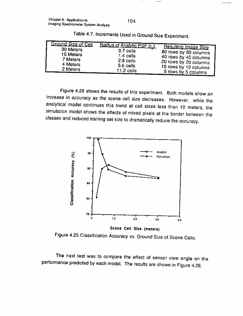
Chapter 4 - Application to
Imaging Spectrometer System Analysis
104
Table 4.7. Increments Used in Ground Size Experiment.
Ground Size of C91130 Meters15 Meters7 Meters4 Meters2 Meters
Radius of Analytic PSF (r=_)_0.7 cells1.4 cells2.8 cells5.6 cells11.2 cells
Resultina Image Size80 rows by 80 columns40 rows by 40 columns20 rows by 20 columns10 rows by 10 columns
5 rows by 5 columns
Figure 4.25 shows the results of this experiment. Both models show an
increase in accuracy as the scene cell size decreases. However, while the
analytical model continues this trend at cell sizes less than 10 meters, the
simulation model shows the effects of mixed pixels at the border between the
classes and reduced training set size to dramatically reduce the accuracy.
o
=...
oo
<C
c0
0lo
5
lOO
95
9O
85
8O
75
Analytic
Simulation
i i |
0 10 20 30 40
Scene Cell Size (meters)
Figure 4.25 Classification Accuracy vs. Ground Size of Scene Cells.
The next test was to compare the effect of sensor view angle on the
performance predicted by each model. The results are shown in Figure 4.26.
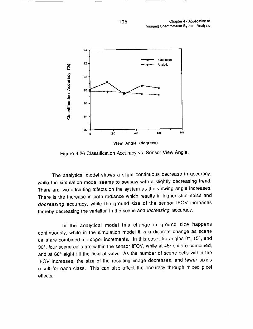
105 Chapter 4 - Application toImaging Spectrometer System Analysis
94
92A
>,_¢)
9o-!
'_ 88co
u 86
_ 84
82
Simulation
...... 9 ...... Analytic
0 20 40 60 80
View Angle (degrees)
Figure 4.26 Classification Accuracy vs. Sensor View Angle.
The analytical model shows a slight continuous decrease in accuracy,
while the simulation model seems to seesaw with a slightly decreasing trend.
There are two offsetting effects on the system as the viewing angle increases.
There is the increase in path radiance which results in higher shot noise and
decreasing accuracy, while the ground size of the sensor IFOV increases
thereby decreasing the variation in the scene and increasing accuracy.
In the analytical model this change in ground size happens
continuously, while in the simulation model it is a discrete change as scene
cells are combined in integer increments. In this case, for angles 0°, 15 °, and
30 °, four scene cells are within the sensor IFOV, while at 45 ° six are combined,
and at 60 ° eight fill the field of view. As the number of scene cells within the
IFOV increases, the size of the resulting image decreases, and fewer pixels
result for each class. This can also affect the accuracy through mixed pixel
effects.
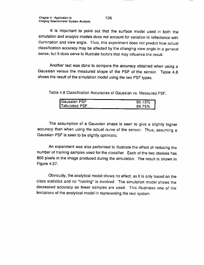
Chapter 4 - Application to
Imaging Spectrometer System Analysis
106
It is important to point out that the surface model used in both the
simulation and analytic models does not account for variation in reflectance with
illumination and view angle. Thus, this experiment does not predict how actual
classification accuracy may be affected by the changing view angle in a general
sense, but it does serve to illustrate factors that may influence the result.
Another test was done to compare the accuracy obtained when using a
Gaussian versus the measured shape of the PSF of the sensor. Table 4.8
shows the result of the simulation model using the two PSF types.
Table 4.8 Classification Accuracies of Gaussian vs. Measured PSF.
GaussianPSF 90.15% JTabulated PSF 89.75%
The assumption of a Gaussian shape is seen to give a slightly higher
accuracy than when using the actual curve of the sensor. Thus, assuming a
Gaussian PSF is seen to be slightly optimistic.
An experiment was also performed to illustrate the effect of reducing the
number of training samples used for the classifier. Each of the two classes has
800 pixels in the image produced during the simulation. The result is shown in
Figure 4.27.
Obviously, the analytical model shows no effect, as it is only based on the
class statistics and no "training" is involved. The simulation model shows the
decreased accuracy as fewer samples are used. This illustrates one of the
limitations of the analytical model in representing the real system.
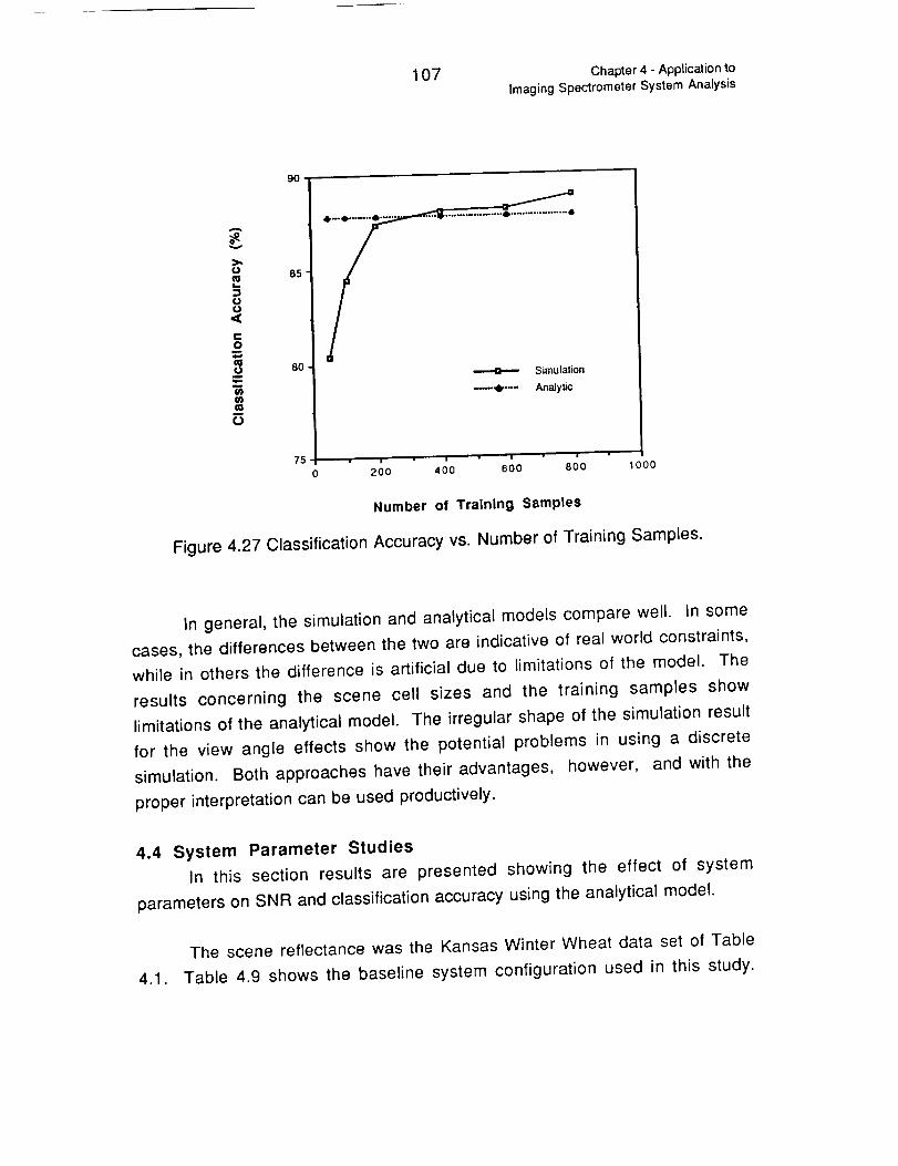
107 Chapter 4 - Application to
Imaging Spectrometer System Analysis
9o
o
2
o
o
(a
85
8O
75
4b •
Simulalion
_, .... Analytic
i i • i
200 400 600 800 1000
Number of Training Samples
Figure 4.27 Classification Accuracy vs. Number of Training Samples.
In general, the simulation and analytical models compare well. In some
cases, the differences between the two are indicative of real world constraints,
while in others the difference is artificial due to limitations of the model. The
results concerning the scene cell sizes and the training samples show
limitations of the analytical model. The irregular shape of the simulation result
for the view angle effects show the potential problems in using a discrete
simulation. Both approaches have their advantages, however, and with the
proper interpretation can be used productively.
4.4 System Parameter Studies
In this section results are presented showing the effect of system
parameters on SNR and classification accuracy using the analytical model.
The scene reflectance was the Kansas Winter Wheat data set of Table
4.1. Tab(e 4.9 shows the baseline system configuration used in this study.

Chapter 4- Application to 1 08Imaging Spectrometer System Analysis
Table 4.10 shows the parameters that were varied and the range of their
variation. Figures 4.28 through 4.51 show the results of these experiments.
Table 4.9 System Configuration for Parameter Studies.
SceneSurface Meteorological RangeAtmospheric ModelHaze ParameterDiffuse Constant
Solar Zenith AngleView Zenith AngleAcross and Down Scene Spatial Correlation
_z.ea3._.gf_(HIR iS Model)Spatial Radius (analytical model ro)Read Noise LevelShot Noise LevelIMC Gain StateRelative Calibration ErrorAbsolute Radiometric ErrorRadiometric Resolution
Processing! Feature SelectionI
16 Km1976 US Standard
Rural Extinction0.8430 °
0 °0.6
1.4 Scene Cells
NominalNominal
1O.5%
O%12 Bits
First 6 Features of Table 4.5I
Table 4.10 Parameters Studied and Their Variation in Section 4.4.
I
Spatial CorrelationMeteorological RangeSolar Zenith AngleView Zenith AngleSensor IFOV On a SideShot Noise FactorRead Noise FactorIMC Gain StateNumber of BitsRelative Calibration ErrorAbsolute Radiometric ErrorNumber of Features
i
0, 0.15, 0.30, 0.45, 0.60, 0.75, 0.902, 4, 8, 16, 32 Km0 °, 15 °, 30 °, 45 °, 60 °0 °, 15 °, 30 °, 45 °, 60 °1,2, 4, 8, 16 Scene Cells0, 0.5, 1.0, 2.0, 4.00, 0.5, 1.0, 2.0, 4.01,2,4,86,8,10,12,14,160, 0.5, 1.0, 2.0, 4.0 %-10, -5, -2, 0, 2, 5, 10 %
1 through 16

109 Chapter 4 - Application to
Imaging Spectrometer System Analysis
"ov
O
¢8
o
Z
6E¢=r,
6O
5O
4O
30
_o o"
°,,_.°°°°- °41_'°'°
9o_ °°
e
i
Ii
i20 • i | |
0.0 0_2 0.4 0.6 0.8.0
Spatial Correlation
Figure 4.28 Effect of Spatial Correlation (p= Px= Py) on SNR.
Voltage SNR
Power SNR
>,,tj
t,.)O,<
¢O,t,,,=catj
¢tJ
100.4
95
90
85
80
75
70
65
6o | | |
012 0.4 0.6 0.8_ O
.0
Spatial Correlation
Figure 4.29 Effect of Spatial Correlation (p= Px= Py) on Classification Accuracy.

Chapter 4 - ApplicationtoImaging Spectrometer System Analysis
110
0
e=
o
0Z
6
¢=r-
80
5O
4O
3O
4 "q._=_==. =====================
O** 4'
i| • j !
0 10 20 30 40
Meteorological Range (Kin)
Figure 4.30 Effect of Meteorological Range on SNR.
Voltage SNR
Power SNR
100"
A
v
PO¢J
c-o7-,
o
95
9O
85
8O
75
70
65
6O
0 O | • !1 20 30 40
Meteorological Range (Kin)
Figure 4.31 Effect of Meteorological Range on Classification Accuracy.

111 Chapter 4 - Application to
Imaging Spectrometer System Analysis
0
o¢o
Z6
c
O'J
6o
5O
40,
1,-°-°--°_- _._..
30
o ' '0 2 40 60 80
Solar Zenith Angle (degrees)
Figure 4.32 Effect of Solar Zenith Angle on SNR.
•"---'-B-"--- Voltage SNR
.... e- -- Power SNR
100,
A
>,,,¢J.=oo
om
o
95
gO
85I ,
8O
75
70
65
6O
0 O | !2 40 60 80
Solar Zenith Angle (degrees)
Figure 4.33 Effect of Solar Zenith Angle on Classification Accuracy.

Chapter 4 - Application to
Imaging Spectrometer System Analysis
112
6O
A
m"ov
O
n-
=O
Z
6"t'
e=e-O}
5o
4O
3O
JeL
=°° .... "= =''''='"=41_.=
"='''--e%
O i i0 2 40 60 80
Sensor Zenith Angle (degrees)
Figure 4.34 Effect of Sensor Zenith Angle on SNR.
Voltage SNR
Power SNR
100
95,
A
v 9O
0
65o
<_ 8o
c0
"" 75oq,,.
(n 70
¢Q
O65,
6O
0
With Pixel Scaling
---,e. ..... Without Pixel Scaling
.t.........-.---"B
_='° "_'°4
| !2 40 60 80
Sensor Zenith Angle (degrees)
Figure 4.35 Effect of Sensor Zenith Angle on Classification Accuracy.
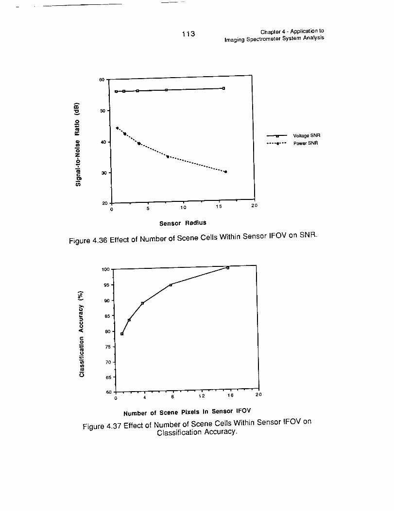
113 Chapter 4 - Application to
Imaging Spectrometer System Analysis
6o
A
in"o
om
5o
4Oo_
o
c_
c 3O
2O
4P,a
, k0 10 15 20
V_ge SNR
.... e-*- PowerSNR
Sensor Radius
Figure 4.36 Effect of Number of Scene Cells Within Sensor IFOV on SNR.
v
o
e,,O
w
8m
100
95
9O
85
80
75
70
65
6O• | • ! I •' "" • I •
4 8 12 16 20
Number of Scene Pixels In Sensor IFOV
Figure 4.37 Effect of Number of Scene Cells Within Sensor IFOV onClassification Accuracy.

Chapter 4 - Application to
Imaging Spectrometer System Analysis
114
0n
o
ou
¢11I=
6O
50
40
.... ,,q .... •°ll_=..**m • "'=_-i..°=_..===_=mQ=" •
3O
0 ; _ ; ;
Shot Noise Factor
Figure 4.38 Effect of Shot Noise (Nominal = 1.0) on SNR.
VoJlage SNR
Power SNR
100
95A
90 ¸
O¢==- 85
O¢J
'_ 8O
e,.o
75,O
Qj=
w 70-w
° :]o i • i i
2 3 4 5
Shot Noise Factor
Figure 4.39 Effect of Shot Noise (Nominal = 1.0) on Classification Accuracy.

115 Chapter 4 - Application to
Imaging Spectrometer System Analysis
7o
A
m
v
_o
o
o=,,
e-
6O
5o
0 2 3 4
-'--'m'-'- Voltage SNR
.... • Q"" Power SNR
Read Noise Factor
Figure 4.40 Effect of Read Noise (Nominal = 1.0) on SNR.
100
A
v
>,L
.=ou
c0
u
u)
95
80
85
80-
75-
70
65
6O
i1
• i i i •0 2 3 4 5
Read Noise Factor
Figure 4.41 Effect of Read Noise (Nominal = 1.0) on Classification Accuracy.

Chapter 4 - Application to
Imaging Spectrometer System Analysis
116
7O
m'¢1
O
OW
OZ
6
¢g
O'J
6O
5O
4o
8o ,f
t, B
e _ _
#l,
Q
i11 I •; , 6 ; ,o
IMC Gain State
Figure 4.42 Effect of IMC Gain State on SNR.
Voltage SNR
Power SNR
A
v
>,o
.=.,I
cO
om
elol¢=
(3
lO0
95,
9O
8s _
75-
70
65
6O
0e i i i
2 4 6 8 10
IMC Gain State
Figure 4.43 Effect of IMC Gain State on Classification Accuracy.

117 Chapter 4 - Application to
Imaging Spectrometer System Analysis
m.1ov
o
o¢/Jo
Z
Ec
6o
5O
4O
3O
---'3 t- "1
...... .Q ....... • ....... •
.o°Z
o,oO
o,oO
20 • w • | - t • i • | • !
4 6 8 10 12 14 16
Voltage SNR
.... e--- PowerSNR
Number of Bits
Figure 4.44 Effect of Radiometric Resolution on SNR.
A
v
u
<
c0
om
t/j
100-
95
90
85
8O
75
70
65"
6O
4
.-.= _.
! • i • i . i . i • !
6 8 10 12 14 16
Number of Bits
Figure 4.45 Effect of Radiometric Resolution on Classification Accuracy.

Chapter 4 - Application to
Imaging Spectrometer System Analysis
118
6O
A
m'ov
Owo=m
¢g
o
Z
6"7
!
t,t3
5O
40,
3OI q
o ; 2 3 ,' 5
Relative Calibration Error (%)
Figure 4.46 Effect of Relative Calibration Error on SNR.
Voltage SNR
Power SNR
100
A
v
tj
t_u
<
cO
m
um
m
ca
¢.)
95
9O
85
8O
75
70
65
6Ol I • I I
0 1 2 3 4 5
Relative Calibration Error (%)
Figure 4.47 Effect of Relative Calibration Error on Classification Accuracy.
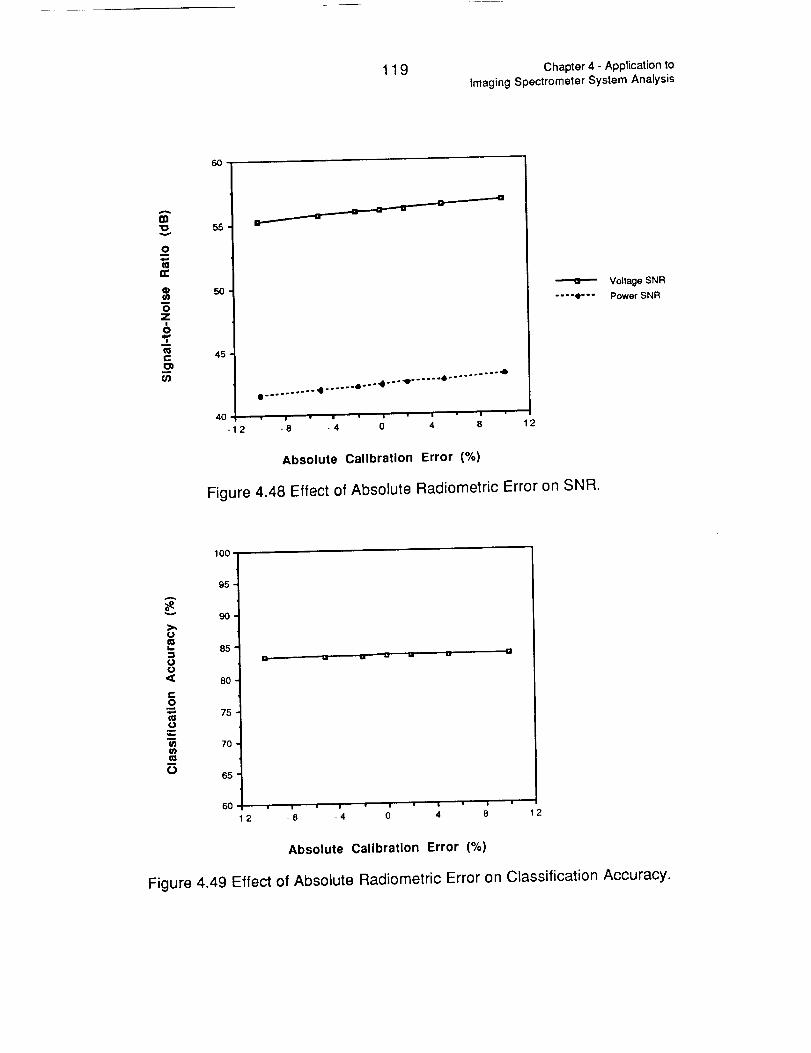
119 Chapter 4 - Application to
Imaging Spectrometer System Analysis
6o
rn"o
0q,.*
t_n-
o
m
0Z
m
coe-
cn
55
5O
45
40
i
• ...... •...•-°-'9 ...... • .......... 4
! • | • ! • | • I •
2 -8 -4 0 4 8
Voltage SNR
.... Q"" Power SNR
Absolute Calibration Error (%)
Figure 4.48 Effect of Absolute Radiometric Error on SNR.
100
A
v
>.¢.)
L
:3
CJ,<
t-O
Ca
t'g
t,.)
g5
gO
85
80
75
7O
65
6O
-' 2
• ' I • I • i • | • I ' •
-8 -4 0 4 8 2
Absolute Calibration Error (%)
Figure 4.49 Effect of Absolute Radiometric Error on Classification Accuracy.

Chapter 4 - Application to
Imaging Spectrometer System Analysis
120
Am"¢3
ow
oca
Z6E(ai=¢3}
6o
5o
40,
o_" °° =" =- o .... = ... .= .°
oo
I30 • • • , . I
Number of Features
Figure 4.50 Effect of Number of Processing Features on SNR.
Voltage SNR
Power SNR
100
v
oo
cO
(ao
t_
m
tO
95
90,
85
80
75
70
65,
6O
55
5O
0= • •
4 8 12 16
Number of Features
Figure 4.51 Effect of Number of Processing Features on Classification Accuracy.

121 Chapter 4 - Application toImaging Spectrometer System Analysis
In computing the SNR values, the method described in section 2.3.4 of
chapter two for a feature was extended for combining all of the features and
computing one value. Also, in computing the power SNR, the weighting
function W s described in chapter three was used to modify the class variances.
The reflectance statistics used in these computations were for the combined
data set. The results of these experiments are summarized in Table 4.11.
Table 4.11 Summary Results for System Parameter Experiments.
System Parameter(Increasing)
Scene
Spatial CorrelationMeteorological RangeSolar Zenith AngleView Zenith Angle
SensorSensor RadiusShot NoiseRead NoiseIMC GainRadiometric ResolutionRelative Calibration ErrorAbsolute Radiometric Error
ProcessingNumber of Features
Figures
4.28, 4.294.30, 4.314.32, 4.334.34, 4.35
4.36, 4.374.38, 4.394.40, 4.414.42, 4.434.44, 4.454.46, 4.474.48, 4.49
4.5O, 4.51
VoltageSNR
No ChangeIncrease
DecreaseDecrease
No ChangeDecreaseDecreaseIncreaseIncrease
DecreaseIncrease
Increase
PowerSNR
IncreaseIncrease
DecreaseDecrease
DecreaseDecreaseDecreaseIncreaseIncrease
DecreaseIncrease
Increase
Accuracy
DecreaseIncrease
DecreaseIncrease
IncreaseDecreaseDecreaseIncreaseIncrease
DecreaseIncrease
Increase
In Figures 4.52 and 4.53, the results of this section are displayed in a
scatter plot to show the relationships between classification accuracy and
signal-to-noise ratio. As can be seen, there is no direct relationship. While
there appears a significant trend of higher classification accuracy resulting from
higher SNR, it is not always the case.
The spatial correlation and sensor IFOV radius are cases in point.
While their variation had a significant effect on both classification accuracy and
power SNR, the effect was opposite. These spatial parameters come into the
noise model only through the modification of the signal covariance matrix thus
there is no effect on voltage SNR.

Chapter 4 - Application to
Imaging Spectrometer System Analysis122
¢==_-,i
,ll
l=0
m
i
IO
Ig
'°°"t| [] 0B/
p • []70
8O
5O
40 50 60 70
Voltage SNR (dB)
Figure 4.52 Accuracy vs. Voltage SNR for System Parameter Experiments.
A
o
m 8ouo<
e-o
¢uomle.
¢o
100 _,
70,
6O
5O
'l=
".=JII _1_ Ill•g=
o Q[]
[] []
[]
[]
[]
i • I0 • i • i • i °tO 2 30 40 50 60
Power SNR (dB)
Figure 4.53 Accuracy vs. Power SNR for System Parameter Experiments.

123 Chapter 4 - Application to
Imaging Spectrometer System Analysis
These results are mostly intuitively appealing, except for the sensor view
angle. Figure 4.35 contained two curves. The one labelled "with scaling" was
obtained using the 1/cos(ev=ew)scaling of the ground size of the sensor IFOV as
0view was changed. The other curve labelled "without scaling" did not. It shows
the effects due solely to the decreased atmospheric transmittance and
increased path radiance. Thus, it seems the increase in accuracy due to the
IFOV scaling overrides the decrease due to the atmospheric effects. Of course,
this experiment assumes a Lambertian surface reflectance and no effects due to
field size and mixed pixels. Also, the atmosphere chosen was relatively clear.
In the next section results are presented to show that in hazier atmospheres, the
effect of the atmosphere on view angle is much more pronounced.
4.5 Interrelated Parameter Effects
In this section results showing the interrelated effects of parameters are
presented. The analytical model is again utilized and the system configuration
is as defined in section 4.4. The parameters studied and their variation are
given in Table 4.12 below.
Table 4.12 Parameter Interrelationship Studies.
Meteorological Range and Sensor View Angle (0sola r = 0°)
Meteorological Range and Sensor View Angle (0sola r = 30 °)
Meteorological Range and Sensor View Angle (esola r = 60 °)Spatial Correlation and Sensor IFOV SizeMeteorological Range and Shot NoiseMeteorological Range and Read NoiseMeteorological Range and IMCMeteorological Range and Number of BitsMeteorological Range and Noise Sources AloneSolar Zenith Angle and Shot NoiseSensor View Angle and Shot NoiseSolar Zenith Angle and IMCSensor View Angle and IMCMeteorological Range and Number of Features
Solar Zenith Angle and Number of Features

Chapter 4 - Application to 124Imaging Spectrometer System Analysis
10o
A
v
ums._
OtJ
COm
m
ma
O
95
9O
85
8O
75 "''-'''''''''''''''''-
7O
6O
55
5O
0• i • i • a • i • | • i !
10 20 30 40 50 60 70
•----a---- 32Km
--.,0 .... 16 Km
.... I--- 8 Km
---ql--- 4Kin
.... I.-- 2 Km
View Zenith Angle (degrees)
Figure 4.54 Effect of Meteorological Range and View Angle for esolar = 0°-
A
v
i--
g
cO
i
o
100
95-
9O
85
75 "
70
65
60-
55
50
0
.a'"--
----------- • ----....... • ---..-..... • ---........•
• | • i • | • ! • i • i •
10 20 30 40 50 60 70
32 Km
.... •4).... 16 Km
.... n--- 8 Km
---ql--- 4 Km
.... II--. 2 Km
View Zenith Angle (degrees)
Figure 4.55 Effect of Meteorological Range and View Angle for esola r = 30 °.

125 Chapter 4 - Application toImaging Spectrometer System Analysis
=Oo
CO
t_
m¢Q
O
100
95
9O
85
8o
75
70,
65 -
9o.
55
5O
45
40
"--'_" ........ ----b... ---.-b..... "°-l.°
"b...II
• I " I • I " I " ! ' !
0 10 20 30 40 50 60 70
32 Km
....... d)...... 16 Km
.... l--- 8 Km
---e--- 4 Km
.... ='-- 2 Km
View Zenith Angle (degrees)
Figure 4.56 Effect of Meteorological Range and View Angle for esolar = 60°.
100
95A
o9°
.-LOO< sscO
mo 80
m
_ 7s
:':,...... i, =...... =" ' -=.
•, _,,. ... \... \
• *4 •
_ "t., "% ''_._, "-. "=, \ \
•-., -,_ ",., _\
\
-2.',)° _"_''U
70 # t • ' r i •
0.0 0-:_ 0.4 0.6 0.8 1.0
----o----. 16
....... ,e.;.... 8
.... I1--- 4
---e--- 2
.... in,-, 1
Spatial Correlation Coefficient
Figure 4.57 Effect of IFOV Size (in Scene Cells) and Spatial CorrelationCoefficient.

Chapter 4 - Application to
Imaging Spectrometer System Analysis
126
10o
95 ¸
A
85-(.,taIk=
:3 80,
0
75
t=0 7O
8-- 65_4='=
(oe_¢= 6O
55
5O
"''° ='°" "''''='''' '''' .... *'---.=k= ....i 1 • • 4
I i • •
| !; 2 3
......,e.....,
---=m-=-
....I...
Shot Noise Factor
Figure 4.58 Effect of Meteorological Range and Shot Noise.
32 Krn
16 Krn
8 Km
4 Km
2 Km
A
>,l#
oo
o¢go
t_
0
_IB,_ "--..o..=. ""'ql)
70 "'--..
60
50
40
".,
i i i0 2 3 4 5
....... "qD'"....
----I---
.... I.--
Read Noise Factor
Figure 4.59 Effect of Meteorological Range and Read Noise.
32 Km
16 Km
8 Km
4 Km
2 Km

127 Chapter 4 - Application to
Imaging Spectrometer System Analysis
v
o
¢to
cO
t_o
¢o
¢o
O
90
85
8O
75
70
65
S
!!
tI
----'B-" IMC,,8
..... ,e ..... IMC-4
.... B'" IMC-2
---t -=" IMC=I
6O • | |
1 "_u 20 30 40
Meteorological Range (Km)
Figure 4.60 Effect of Meteorological Range and IMC.
>,,oPoo
o
o
100
9O
8O
7o
60
_- 50(/3
tJ 4O
3O
_ oo_- o_ _-
i1_ Ill
o #• ... ........... • •
• s,,e''
G • °
i._ •S
•1
#"
s*
•°
j"
• i • | • i • i • !
6 8 10 12 14 16
32 Km
....... 4)...... 16 Km
.... 1--- 8 Km
--°_)--- 4 Km
.... • .-- 2 Krn
Number of Bits
Figure 4.61 Effect of Meteorological Range and Radiometric Resolution.

Chapter 4 ° Application to
Imaging Spectrometer System Analysis
128
go
85
>,O 8O
O
75
C_o,,d
_ 7o
WIn
_ 6s
im
O
0 1 20 30 40
-- --Pt -- No Noise
...... o .... Ouant
- - - -O- -- Shot
---I--- Read
-'- O" - • Cal - 2%
Meteorological Range (Km)
Figure 4.62 Effect of Meteorological Range and Various Noise Sources Alone.
84
83
oe=L_
:= 82rjO<
O 81
¢1o
m 80rO
7g
.,%
,,b°
! !
Solar Angle
0o
...... _ ...... 15 °
.... l- - - 30 °
... _. -. 45 °
.... II,-, 60 °
Shot Noise Factor
Figure 4.63 Effect of Solar Angle and Shot Noise.

129 Chapter 4 - ApplicationtoImaging Spectrometer System Analysis
86
A
v
>,o
¢1oo
¢-o
o
85
84
83
82
81
0 2 3 4 5
View Angle
60"
....... 4)...... 45 °
.... i... 30 °
---Q--- 15 °
.... III • - • 0 °
Shot Noise Factor
Figure 4.64 Effect of View Angle and Shot Noise.
86
A
>,
m2,--
o<
cO
cao
_D
85
84
83
82
81
..............,....._..................._................t ...............,=i- °-_--o.--i...o.O..o
11
2 40 60 80
--o-ieo--
Solar Zenith Angle (degrees)
Figure 4.65 Effect of Solar Angle and IMC Gain State.
IMC=8
IMC=4
IMC=2
IMC=I

Chapter4- Applicationto
Imaging Spectrometer System Analysis
130
o.=oo
c0
90
. ./....""."'.."EC'.." T'.".'--.----- ...... .
82
8O
0 ' '0 2 40 60 80
IMC=8
--.,e ...... IMC=4
.... I- - - IMC,,,2
---,e--- IMC=I
View Angle (degrees)
Figure 4.66 Effect of View Angle and IMC Gain State.
100
9oA
8O>,_U
'- 70
OU
'_ 6O
c-O
50'mo
40e_(=
O3o
2o • I
1; ,_ - .r "_
/f /Di ill..I "'ll
, ill #
p. II
I
Io
iI
| . . I • • • • I • • • • i • • • • i • •
4 8 t2 16
32 Km
....... .O...... 16 Km
.... I--- 8 Km
=--e--- 4 Km
.... I.-, 2 Km
Row Numbers
Figure 4.67 Effect of Meteorological Range and Number of Features.

131 Chapter 4 - Application to
Imaging Spectrometer System Analysis
lOO
v
>,,
¢=
8O
0 70
Mo_=w
5O
4 8 12 16
0o
-- --Q. -- 60 o
Number of Features
Figure 4.68 Effect of Solar Angle and Number of Features.
The results of these experiments are discussed in the following
paragraphs.
Figures 4.54 through 4.56 help understand the relationships between
meteorological range, sensor view angle, and solar zenith angle. In clear
atmospheres, the increase in accuracy due to the geometry of higher view
angles is evident. However, as the atmosphere becomes hazy, the decreased
signal levels and increased path radiance become dominant and accuracy is
then decreased for higher view angles. The effects due to the atmosphere are
seen to be more significant for higher solar zenith angles.
Figure 4.57 shows a complex relationship between the spatial correlation
of scene cells, and the number of cells in a sensor IFOV side. With increasing
correlation, the accuracy for small cells (many cells per IFOV side) falls sharply
before decreasing at a constant rate, while the accuracy for large scene cells
(few cells per IFOV side) remains constant before falling sharply at high

Chapter 4 - Application toImaging Spectrometer System Analysis
132
correlations. While this result shows the tradeoffs on classification accuracy of
scene cell size and spatial correlation for constant sensor IFOV, it is interesting
to consider this in the light of the results of Table 2.2. There it was shown that
spatial correlation decreases with increasing scene cell size. Thus, for typical
remote sensing data sets large scene cells have low spatial correlation, while
small cells have high correlation. These tradeoffs form an imaginary horizontal
line across Figure 4.57 and indicate that classification accuracy is relatively
independent of scene cell size.
Figures 4.58 and 4.59 show that the effects due to increased noise are
more significant in hazy atmospheres, while Figure 4.60 shows the
improvement by using IMC to be greater in hazy atmospheres. Figure 4.61
demonstrates how the increase in quantization error of fewer radiometric bits
can be more significant in hazy atmospheres.
In Figure 4.62, it can be seen that the read noise and relative calibration
errors are more significant for all meteorological ranges, while the effect of shot
noise is greater at low ranges due to the increase in path radiance. It is
interesting to compare the effect of the atmosphere with no noise sources
present shown here with that of Landgrebe and Malaret (1986). Their result
showed the atmosphere had no effect when no sensor noise was present, while
Figure 4.62 shows a significant effect. The difference in these results is due to
the path radiance model used in this report. Malaret's model considered path
radiance as a constant additive source, while the model used here is
dependent upon the surface reflectance. Figure 4.69 shows the effect of the
atmosphere with and without sensor noise for the system model modified to
remove the surface reflectance dependence on path radiance. As can be
seen, the atmosphere has little effect on accuracy when this dependence is
removed. It is known that path radiance is dependent upon surface reflectance
in the real world, thus the results shown in Figure 4.62 are judged to be more
realistic.

133 Chapter 4 - Application to
Imaging Spectrometer System Analysis
Qo
88A
86o
u 84u
c0 82
u"- 80
0 78
76
•.---B--.- No Sensor Noise...... "4)..... Nominal Sensor Noise
0 10 20 30 40
Meteorological Range (Kin)
Figure 4.69 Effect of Atmosphere With/Without Noise For Path Radiance ModelWith No Surface Reflectance Dependence.
Figures 4.63 and 4.64 contain some interesting results. In Figure 4.63,
the effect of shot noise is seen to be greater at high solar zenith angles, while in
Figure 4.64, just the opposite is seen for high view angles. In both cases, the
effect due to the shot noise alone is to decrease accuracy more at higher
angles, but for the view angle case the increase in accuracy due to the
geometry overrides the shot noise effect.
Figure 4.65 shows how the IMC can be used to overcome the
combination of low signal levels and high read noise to actually increase
accuracy at high solar zenith angles. In Figure 4.66, a similar effect is seen as
the IMC increases accuracy by a greater amount at high view angles.
Figures 4.67 and 4.68 show how, up to a point, more features can be
used in classification to overcome the effects of the atmosphere or solar angle.

Chapter 4 - ApplicationtoImaging Spectrometer System Analysis
134
However, it can be seen that the accuracy increases level out after a certain
number of features and increases beyond that level are not significant.
Overall, the results of these experiments show the complex interaction of
system parameters in determining their effect on classification accuracy. This
demonstrates the importance of considering the interdependence of parameters
when considering their specification in the design of a remote sensing
experiment.
4.6 Feature Selection Experiments
Several sets of six features (shown in Table 4.13) were used to evaluate
their classification performance for a variety of system parameter variations and
scenes. This section presents the results of these experiments.
Table 4.13 Wavelength Bands Combined for the Various Feature Sets. TheVarious Feature Sets are Defined as SFD = Spectral Feature Design Algorithm,TM = Landsat Thematic Mapper, WSNR - Wide Signal-to-Noise Ratio, NSNR =Narrow Signal-to-Noise Ratio, SSFD = Single Band Spectral Feature, SSNR =Single Band Signal-to-Noise Ratio.
Feature, i
123456
SFD0.52-0.660.66-0.840.70-0.921.48-1.641.98-2.202.20-2.40
TM0.45-0.52
0.52-0.600.63-0.690.76-0.901.45-1.752.08-2.35
WSNR
0.40-0.700.77-0.901.00-1.101.15-1.301.50-1.741.97-2.40
NSNR0.51-0.560.81-0.861.02-1.071.20-1.251.59-1.642.16-2.21
SSFD
0.59O.750.811.562.102.30
SSNR0.540.841.041.111.612.19
The SNR features were chosen based upon spectral regions of high
SNR. These various sets were chosen to see how classification accuracy and
combined signal-to-noise ratios compared. Figure 4.70 shows the voltage and
power SNR for the various feature sets and the combined reflectance statistics
of the data set in Table 4.1, while Figure 4.71 shows the resultant classification
accuracy for the baseline system of Table 4.9.

135 Chapter 4 - Application to
Imaging Spectrometer System Analysis
A
m"o
;¢¢/)
2o
lO
[] Voltage SNR
[] Power SNR
SFD TM _ NSNR SSFD SSNR
Feature Set
Figure 4.70 Voltage and Power SNR for the Various Feature Sets of Table 4.13.
85
v
o¢= 8O
o
e,,o
_ 75
w
w
70
SFD TM WSNR NSNR SSFD SSNR
Feature Set
Figure 4.71 Classification Accuracy for the Various Feature Sets of Table 4.13.

Chapter 4 ° Application to
Imaging Spectrometer System Analysis
136
In this case, the SFD features performed the best for this data set, even
though they did not have highest SNR. However, since they were derived from
the data used to generate the scene, it is expected that they perform well.
Several experiments were run to compare the performance of the various
feature sets over varying scene conditions. Figures 4.72, 4.73, and 4.74 show
the classification performance of the feature sets for various meteorological
ranges, solar zenith angles, and view angles.
90
A
6o
o
70¢.)O
CO 6O
8q.
M_ N3,
0
?
o 30 ,o
SF'D
...... •e...... TM
.... m--- WSNR
-'-t -°" NSNR
.... m.-" SSFD
----a"-- SSNR
Meteorological Range (Kin)
Figure 4.72 Feature Set Performance vs. Meteorological Range.
From these curves, it can be seen that the features derived from high
SNR regions are less susceptible to changes in the scene parameters.
However, they give overall less accuracy than the features obtained from the
SFD algorithm. Also, the features that are obtained from only one spectral band
perform poorly under all conditions.

137 Chapter 4 - Application to
Imaging Spectrometer System Analysis
A
P
u
co(u
u
coM
O
84
82
8O
78
76
74
72
, .......... t ................ • ................. t'.o--._ ........ *4
i I i
0 20 40 60
SF-E)
....... •ql...... TM
.... i""
"--t''" NSNR
.... m'-" SSFD
-- --IT -- SSNR
8O
Solar Zenith Angle (degrees)
Figure 473 Feature Set Performance vs. Solar Angle
A
t.).=
p,O,,i,ii
m
C)
8S
84
82
80
78
76
74
......... 1D° "d,
.....l_ol #
......... "1 ......... m'"'" .-4
.__.._...._......----
.......... _. E-.-. E_.._._._.._.:_.,,,,."- -o'o
0 | i0 2 40 60 80
.... U...
---qlm-- -
I n_ I
Sensor Zenith Angle (degrees)
Figure 474 Feature Set Performance vs. View Angle.
SFD
TM
NSNR
SSFD
SSNR

Chapter 4 - Application to 138Imaging Spectrometer System Analysis
The robustness of the spectral feature design algorithm was then studied
by comparing the accuracy of the various feature sets in classifying a scene
created from a different data set than that from which the features were derived.
A scene was created from reflectance data of three varieties of spring wheat.
Table 4.14 gives the specific fields from the LARS field data base.
Table 4.14. Classes and fields used to compute statistics for the Spring Wheattest scene. The data is from Hand County, South Dakota, on July 26, 1978.
Classes
Spring Wheat
SW 1809
SW Mix
Field118154199291292
296303
75281
Number of Observations1329282816
Total = 1142858
Total = 861355
Total = 68
The system configuration was as shown in Table 4.9. Figure 4.75 shows
the voltage and power SNR of the Spring Wheat test scene for the various
feature sets, while Figure 4.76 presents the resulting classification accuracy.
In all cases, the features formed from the wavelengths used in the
Landsat TM and the ones from high SNR regions performed the best.
Compared to these feature sets, the SFD feature set did not perform as well.

139 Chapter 4 - Application to
Imaging Spectrometer System Analysis
60
5o
A
m1o
rrZul
40
[] Voltage SNR
[] Power SNR
10
SF'D TM W'SNR NSNR SSFD SSNR
Feature Set
Figure 4.75 SNR for Various Feature Sets and SW Variety Scene.
SFD TM WSNR NSNR SSFD SSNR
Feature Set
Figure 4.76 Classification Accuracy for Various Feature Sets and SW VarietyScene.

Chapter 4 - Application to 140Imaging Spectrometer System Analysis
These results imply that over varying scenes the features derived from
the reflectance of a different crop type perform less well at classification than
features derived from signal-to-noise regions of the instrument, or even the
wavelength bands used in the Thematic Mapper. This is not surprising since
the SFD procedure is intended to be case-specific; it is intended to provide
features optimal for its design case, as compared to being optimal in the
general case.
4.7 Summary and Conclusions
In this chapter the system models presented in chapters two and three
have been applied to the study of a remote sensing system based on the
proposed imaging spectrometer HIRIS. System performance measured by
signal-to-noise ratios and classification accuracy has been studied under a
variety of system parameter configurations. While the results of these
experiments have been discussed at the end of each of the sections, the
following paragraphs briefly summarize the main conclusions.
In section 4.2 the Signal-to-Noise Ratio (SNR) and Noise Equivalent
Change in Reflectance (NEAp) of HIRIS was studied. The results illustrated
how the atmosphere affects each of the spectral bands, and what noise sources
are the most dominant under a variety of conditions. •Hazier atmospheres were
seen to have more significant effects on the shorter wavelength bands than the
longer wavelengths. Shot noise was seen to be more significant at the high
signal levels at the wavelengths of the VNIR detector array, while read noise
was the dominant noise source in the longer wavelengths of the SWlR array.
Section 4.3 investigated the similarities and differences between the
simulation model of chapter two and the analytical model of chapter three. The
results indicated that the approaches gave similar results, except in cases
where mixed pixels or the training of a classifier were involved.
Section 4.4 presented the results of applying the analytical model to the
study of the individual effect of several parameters on SNR and classification
accuracy. The results generally showed a trend of increased SNR resulting in
increased accuracy, except for parameters involved with spatial variation. Here,

141 Chapter 4 - Application to
Imaging Spectrometer System Analysis
the spatial parameters resulting in lower power SNR gave an increase in
classification by increasing the separability of the classes.
In section 4.5 the interdependence of system parameters was
investigated. Significant relationships were seen between system parameters,
especially those involving pixel size variations and signal dependent noise.
Section 4.6 presented several results comparing various methods of
choosing spectral feature sets under a variety of system conditions. The results
indicated that feature sets based on high SNR were the most robust under
system parameter variations, but feature sets derived from the original
reflectance data were optimum for scenes created from that data.
These results have been presented to show the relative importance of
the system parameters. In no way are these results intended to be used to
predict the actual performance of the system. Rather, they are useful in
discovering the relative effects and tradeoffs in specifying the various
parameters.

Chapter 4 - Application to
Imaging Spectrometer System Analysis142

143 Chapter 5 - Conclusions andSuggestions for Further Work
CHAPTER 5
CONCLUSIONS AND
SUGGESTIONS FOR FURTHER WORK
In pursuing this research, the goals were to: 1) document and model the
remote sensing process from an overall systems perspective; 2) develop a tool
to allow the study of the interrelationships of identifiable system parameters; 3)
apply this tool to the study of optical remote sensing systems.
Chapters one and two described the remote sensing process from a
systems perspective. It was seen to be comprised of three major components:
the scene, the sensor, and the processing algorithms. Modeling of these
components was discussed from a general point of view, and a framework was
described for implementing a subset of these models in a simulation of the
entire system. The simulation used the scene models to produce a spectral
radiance function over a defined scene consisting of various informational
classes arranged spatially. The sensor models then converted this function into
a digital multispectral image, similar to that produced by real sensors. Various
processing algorithms were then applied to this image to extract a performance
measure of the system.
Chapter three presented an alternative to the simulation approach with
the development of a parametric model to describe the remote sensing process.
This model used analytical equations to describe the effects of the various
system parameters.
Each of these approaches are useful as a tool to study remote sensing
systems, and the choice of their use is dependent upon the goal of the study.

Chapter 5 - ConclusionsandSuggestions for Further Work
144
The simulation method is useful in the following example cases.
• The spatial layout of the various classes is of interest.
• A particular scene or image is desired to be simulated under a variety
of conditions.
° An image with desired characteristics is needed for the study of
various processing algorithms.
• One scene needs to have several different sensors applied to it to
compare the resulting images.
• It is desired to use a very accurate and detailed model for the sensor
spatial, spectral, and noise effects.
• It is desired to introduce spatial effects in the scene such as clouds,
shadows, or in the sensor such as geometric distortion or
misregistration.
The parametric model is useful for the following examples.
• Parameter tradeoff studies where detail of models can be sacrificed
for speed of results.
• The scene has a large number of classes with no particular
constraints on spatial layout.
These are only a few of the possible uses of both approaches, but they
are listed to illustrate some of the kinds of studies that are possible under the
modeling framework developed in this report.
Chapter four presented a detailed study of the system performance of a
future imaging spectrometer. The goals were to Svaluate the noise and
classification performance of the instrument under a variety of system
configurations. For the majority of the results, the analytical model was
implemented. This allowed the tradeoff study of several parameters to help
determine the interrelationships among them. Although the results were for the
particular instrument and scene defined, the general trends were observed and
are believed to hold for similar systems.

145 Chapter 5 - Conclusions and
Suggestions for Further Work
Some of the significant results of this study of HIRIS include the following.
• Atmospheric visibility and scattered path radiance influence the
sensitivity of the instrument to ground reflectance changes much more
in the visible wavelengths than in the infrared.
• While classification accuracy is usually related directly to SNR, it is
not always the case.
° The effect of the atmosphere on sensor viewing angle varies
significantly with visibility.
• Lower classification accuracies in hazy atmospheres are not only
because of noise sources in the sensor, but also the increased path
radiance scattered from the surface.
° While feature sets chosen from spectral regions of high SNR are
robust across system parameter variations, feature sets derived using
analytical approaches from field databases perform optimally for
scenes created from the data.
The work presented here has been but one step on the road to modeling
and understanding optical remote sensing systems. It has built upon the work
of many previous researchers, and hopefully, will stand as a foundation for
future efforts.
While almost every component of the system model could be improved,
several particular areas deserve to be pointed out. The surface reflectance
model assumption of Lambertian reflectance could be replaced by a description
of the bidirectional reflectance. Embedded within this function should be the
spectral and spatial variation of the reflectance. Another assumption used in
the scene spatial model that needs work is the spatial crosscorrelation between
high spectral resolution reflectance data.
Two aspects of the atmospheric model could be extended. The
relationship between the total surface irradiance and the direct irradiance
needs to be more adequately defined. Also, spatial blurring and spatial
variability of the atmosphere could be implemented.

Chapter 5 - Conclusions andSuggestions for Further Work
146
Geometric distortion and spectral band misregistration could be
implemented in the sensor model.
This simulation approach could be used today to generate realistic high
dimensional multispectral images for use in processing algorithm study. These
may be studies of hyperspectral image display or classification algorithm
development.
These are but a few of the possible extensions and uses of the modeling
approaches. Indeed, it would seem to be an axiom of modeling that one can
always improve one's model, especially when part of the subject is the natural
world.
1 47 List of References
LIST OF REFERENCES
Allen, W.A., T.V. Gayle, and A.J. Richardson, "Plant Canopy Irradiance Specified By DuntleyEquations," Journal Optical Society of America, vol. 60, pp. 372-376, 1970.
Anuta, P.E., "LARSIUniversity of Michigan Aircraft Scanner Data System Parameter IdentificationStudy," LARS Information Note 091470, Laboratory for Applications of Remote Sensing,Purdue University, West Lafayette, IN 47907, September 1970.
Asrar, G., Editor, Theory and Applications of Optical Remote Sensing, Wiley-Interscience, New York, NY, 1989.
Badhwar, G.D., K.E. Henderson, D.E. Pitts, W.R. Johnson, M.L. Sestak, T.Woolford, J. Carnes,"A Comparison of Simulated Thematic Mapper Data and Multispectral Scanner Data forKingsbury County, South Dakota," Proceedings of 1982 Machine Processing ofRemotely Sensed Data Symposium, West Lafayette, IN, 1982.
Badhwar, G.D., W. Verhoef, and N.J.J. Bunnik, "Comparative Study of Suits and SAIL CanopyReflectance Models," Remote Sensing of Environment, vol. 17, pp. 179-195, 1985.
Bartlett, D.S., R.W. Johnson, M.A. Hardisky, and V. Klemas, "Assessing Impact of Off-NadirObservation on Remote Sensing of Vegetation: Use of the Suits Model," Int. J. RemoteSensing, vol. 7, no. 2, pp. 247-264, February 1986.
Biehl, L.L., M.E. Bauer, B.F. Robinson, C.S.T. Daughtry, L.F. Silva, and D.E. Pitts, "A Crops andSoils Data Base for Scene Radiation Research," Proceedings of the 8th InternationalSymposium on Machine Processing of Remotely Sensed Data, pp. 169-177, PurdueUniversity, West Lafayette, IN, 1982.
Billingsley, F.C., "Modelling Misregistration and Related Effects on Multispectral Classification,"Photogrammetric Engineering and Remote Sensing, vol. 48, pp. 421-430,1982
Bird, R.E., "Terrestrial Solar Spectral Modeling," Solar Cells, vol. 7, no. 1-2, pp. 107-118,November 1982.
Carter,V. and J. Schubert,"Coastal Wetlands Analysis From ERTS MSS Digital Data and FieldSpectral Measurements," Proceedings of the Ninth International Symposium on RemoteSensing of the Environment, Ann Arbor, MI, pp. 1241-1260, 1974.
Castle, K.R., R.G. Holm, C.J. Kastner, JM. Palmer, P.N. Slater, M. Dinguirard, C.E. Ezra, R.D.Jackson, and R.K. Savage, "In-Flight Absolute Radiometric Calibration of the ThematicMapper," IEEE Transactions on Geoscience and Remote Sensing, VoI. GE-22, No. 3, pp.251-255, May 1984.
Catanzariti, E., "Satellite Image Understanding Through Synthetic Images," in PictorialAnalysis, ed. R.M. Haralick, pp. 369-383, Springer-Verlag, 1983.

List of References 1 48
Chahine, M.T. "Interaction Mechanisms Within the Atmosphere," Chapter 5 in Manual ofRemote Sensing, 2nd Edition, edited by R.N. Colwell, American Society ofPhotogrammetry, Falls Church, VA, 1983.
Chance, J.E. and W.E. LeMaster, "Suits Reflectance Models for Wheat and Cotton: Theoretical
and Experimental Tests," Applied Optics, vol. 16, no. 2, pp. 407-412, February 1977.
Chandrasekaran, B. and A.K. Jain, "Independence, Measurement Complexity, and ClassificationPedormance," IEEE Transactions on Systems, Man, and Cybernetics, vol. SMC-5, no. 2,pp. 240-244, March 1975.
Chellappa, R., "Stochastic Models in Image Analysis and Processing," Ph.D. Thesis, PurdueUniversity, West Lafayette, IN 47907, August 1981.
Chen, C.-C. T., and D.A. Landgrebe, "Spectral Feature Design In High Dimensional MultispectralData," TR-EE 88-35, School of Electrical Engineering, Purdue University, West Lafayette,IN, August 1988.
Cicone, R.C., W.A. Malila, J.M. Gleason, and R.F. Nalepka, "Effects of Misregistration onMultispectral Recognition," Proceedings of the Symposium on the Machine Processingof Remotely Sensed Data, Purdue University, West Lafayette, IN, pp. 4A-1 to 4A-8, 1976.
Clark, J., and N.A. Bryant, "LANDSAT-D Thematic Mapper Simulation Using Aircraft MultispectralScanner Data," Proceedings of the 15th Environmental Research Institute of MichiganSymposium, 1982.
Colwell, R.N., Editor, Manual of Remote Sensing, 2nd Edition, American Society ofPhotogrammetry and Remote Sensing, Fails Church, VA, 1983.
Cooper, K., J. Smith, and D. Pitts, "Reflectance of a Vegetation Canopy Using the AddingMethod," Applied Optics, vol. 21, pp. 4112-4118, 1982.
Craig, R.G., "The Spatial Structure of Terrain: A Process Signal in Satellite Digital Images,"Proceedings of the Ninth Pecora Remote Sensing Symposium, pp. 51-54, IEEEComputer Society Press, October 1984.
Crane, R.B., W.A. Malila, and W. Richardson, "Suitability of the Normal Density Assumption forProcessing Multispectral Scanner Data," IEEE Transactions on Geoscience Electronics,Vol GE-10, No. 4, October 1972.
Crutchfield, J.P., J.D. Farmer, N.H, Packard, R.S. Shaw, "Chaos," Science, December 1986.
Dave, J.V., "Extensive Datasets of the Diffuse Radiation in Realistic Atmospheric Models withAerosols and Common Absorbing Gases," Solar Energy, vol. 21, pp. 361-369, 1978.
Delp, E.J., R.L. Kashyap, and O.R. Mitchell, "Image Data Compression Using AutoregressiveTime Series Models," Pattern Recognition, vol. 11, pp. 313-323, 1979.
Diner, D.J. and V.V. Martonchik, "Atmospheric Transfer of Radiation Above an InhomogeneousNon-Lambertian Reflective Ground I. Theory," Journal Quant. Spectros. Rad. Transfer,Vol. 31 pp. 97-125, 1984.
Dodd, N., "Multispectral Texture Synthesis Using Fractal Concepts," IEEE Transactions onPattern Analysis and Machine Intelligence, VoI. PAMI-9, No. 5, pp. 703-707, September1987.

149 List of References
Duda, R.O., and P.E. Hart, Pattern Classification and Scene Analysis, John Wiley andSons, New York, NY, 1973.
Elterman, L., "UV, Visible, and IR Attenuation for Altitudes to 50 Km," AFCRL 68-0153, AFCRERP 285, Air Force Cambridge Research Laboratories, Bedford MA, 1968.
Elterman, L., "Vertical Attenuation Model with Eight Sudace Meteorological Ranges, 2 to 13 km,"Report 70-0200, Air Force Cambridge Research Laboratory, Bedford, MA, 1970.
Fischel, D., "Validation of the Thematic Mapper Radiometdc and Geometric CorrectionAlgorithms," IEEE Transactions on Geoscience and Remote Sensing, vol. GE-22, no. 3,pp. 237-242, May 1984.
Foley, D.H., "Considerations of Sample and Feature Size," IEEE Transactions on InformationTheory, Vol. IT-18, No. 5, September 1972.
Fdedlander, B., "On the Computation of the Cramer-Rao Bound for ARMA Parameter Estimation,"IEEE Transactions on Acoustics, Speech, and Signal Processing, vol. ASSP-32, no. 4,pp. 721-727,August 1984.
Fukanaga, K. and T.F. Kdle, "Calculation of Bayes' Recognition Error for Two Multivariate GaussianDistributions," IEEE Transactions on Computers, vol. C-18, no. 3, pp. 220-229, March1969.
Fukanaga, K., Introduction to Statistical Pattern Recognition, Academic Press, 1972.
Ghassemian, H. and D.A. Landgrebe, "An Unsupervised Feature Extraction Method for HighDimensional Image Data Compaction," Proceedings of the Systems, Man andCybernetics Conference, Alexandria, VA October 20-23, 1987.
Gleick, J., Chaos: Making a New Science, Viking Penguin, 1987.
Goetz, A.F.H. and M. Herring, "The High Resolution Imaging Specdrometer (HIRIS) for Eos," IEEETransactions on Geoscience and Remote Sensing, Vol. GE-27, No. 2, pp. 136-144,March, 1989.
Goodman, J.W. Introduction to Fourier Optics, McGraw Hill, 1968.
Haralick, R.M., "Statistical and Structural Approaches to Texture," Proceedings of the IEEE, vol.67, no. 5, pp. 786-804, May 1979.
Herman, S.M. and S.R. Browning, "The Effect of Aerosols on the Earth Atmosphere Albedo,"Journal of Atmospheric Science, vol. 32, pp. 1430-1445, 1975.
Hixson, M.M., M.E. Bauer, and L.L. Biehl, "Crop Spectra From LACIE Field Measurements,"LARS CR 011578, Laboratory for Applications of Remote Sensing, Purdue University,West Lafayette, IN, 1978.
Horn, B.K.P. and B.L. Bachman, "Using Synthetic Images to Register Real Images with SurfaceModels," Communications of the ACM, vol. 21, no. 11, November 1978.
Huck, F.O., R.E. Davis, C.L. Fales, R.M. Aherron, R.F. Arduini, and R.W. Samms, "Study ofRemote Sensor Spectral Responses and Data Processing Algorithms for FeatureClassification," Optical Engineering, vol. 23, no. 5, pp. 650-666, September/October1984.
Hudson, R.D., Jr., Infrared System Engineering, Wiley-lnterscience, New York, NY, 1969.

List of References 1 50
Hughes, G.F., "On the Mean Accuracy of Statistical Pattern Recognizers," IEEE Transactions onInformation Theory, vol. IT-14, no. 1, pp. 55-63, January 1968.
Irons, J.R., K.J. Ranson, and C.S.T. Daughtry, "Estimating Big Bluestem Albedo From DirectionalReflectance Measurements," Remote Sensing of Environment, vol. 25, pp. 185-199,1988.
JPL, "High-Resolution Imaging Spectrometer (HIRIS): Phase A Final Report," JPL D-4782, JetPropulsion Laboratory, California Institute of Technology, Pasadena, CA, November1987. Also, data was obtained from viewgraphs used in a presentation by V. Wright ofJPL on October 6, 1987 to the Imaging Spectrometer Science Advisory Group (ISSAG).
Jensen, J.R., "Urban Change Detection Mapping Using Landsat Digital Data," The AmericanCartographer, vol. 8, pp. 127-147, 1981.
Johnson Space Center, "Modular Multiband Scanner (MMS)", JSC Internal Note No. 74-FM-47,Johnson Space Center, Houston Texas, July, 1974.
Kay, S., "Generation of the Autocorrelation Sequence of an ARMA Process," IEEE Transactionson Acoustics, Speech, and Signal Processing, vol. ASSP-33, no. 3, pp. 733-734, June1985.
Kailalh, T., "The Divergence and Bhattacharyya Distance Measures in Signal Selection," IEEETransactions on Communication Technology, vol. COM-15, no. 1, pp. 52-60, February1967.
Kalayeh, HM., M.J. Muasher, and D.A. Landgrebe, "Feature Selection with Limited TrainingSamples," IEEE Transactions on Geoscience and Remote Sensing, vol. GE-21, no. 4,pp. 434-438, October 1983.
Kaufman, Y.J. and R. S. Fraser, "Atmospheric Effect on Classification of Finite Fields," RemoteSensing of Environment, vol. 15, no. 2, pp. 95-118, March 1984.
Kaufman, Y.J., "Atmospheric Effect on Spatial Resolution of Surface Imagery," Applied Optics,Vol. 23, No. 19, pp. 3400-3408, 1 October 1984.
Kaufman, Y.J., "Atmospheric Effect on the Separability of Field Classes Measured fromSatellites," Remote Sensing of Environment, pp. 21-34, August 1985.
Kerekes, J.P. and D.A. Landgrebe, "A Noise Taxonomy for Remote Sensing Systems," inProceedings of IGARSS '87 Symposium, pp. 903-908, Ann Arbor, MI, 18-21 May, 1987.
Kerekes, J.P. and D.A. Landgrebe, "HIRIS Performance Study," TR-EE 89-23, School ofElectrical Engineering, Purdue University, West Lafayette, IN, April, 1989a.
Kerekes, J.P. and D.A. Landgrebe, "RSSIM: A Simulation Program for Optical Remote SensingSystems," TR-EE 89-48, School of Electrical Engineering, Purdue University, WestLafeyette, IN, August, 1989b.
Kettig, R.L., "Computer Classification of Remotely Sensed Multispectral Image Data by Extractionand Classification of Homogeneous Objects," PhD Thesis, School of ElectricalEngineering, Purdue University, West Lafayette, IN, May 1975. Also available as LARSTR 050975.
Kimes, D.S. and J.A. Kirchner, "Radiative Transfer Model for Heterogeneous 3-D Scenes,"Applied Optics, vol. 21, no. 22, pp. 4119-4129, 15 November 1982.

151 Listof Reference=
Kneizys, F.X., et al., "Atmospheric Transmittance/Radiance: Computer Code LOWTRAN 6,"AFGL-TR-83-0187, ERP No. 846, Air Force Geophysics Laboratory, Hanscom Air ForceBase, MA, August 1983.
Kneizys, F.X., E.P. Shettle, L.W. Abreu, J.H. Chetwynd, G.P. Anderson, W.O. Gallery, J.E.A.Selby, and S.A. Clough, "Users' Guide to LOWTRAN 7," AFGL-TR-88-0177, ERP No.1010, Air Force Geophysics Laboratory, Hanscom Air Force Base, MA, August 1988.
Koziol, J.A., "On Assessing Multivariate Normality," Journal of Royal Statistical Society B, vol. 45,no. 3, pp. 358-361, 1983.
Landgrebe, D.A., "Systems Approach to the Use of Remote Sensing," LARS Information Note041571, Laboratory for Applications of Remote Sensing, Purdue University, WestLafayette, IN 47907, April 1971.
Landgrebe, D.A., L.L. Biehl, and W.R. Simmons, "An Empirical Study of Scanner SystemParameters," IEEE Transactions on Geoscience and Remote Sensing, vol. GE-15, no. 3,pp. 120- 130, July 1977.
Landgrebe, D.A., and E.R. Malaret, "Noise in Remote Sensing Systems: The Effect onClassification Error," IEEE Transactionson Geoscience and Remote Sensing, vol. GE-24,no. 2, March, 1986.
LARS Staff,'Testing the Gaussian Assumption on,_AircraftData," LARS Information Note 040469,Laboratory for Applications of Remote Sensing, Purdue University, West Lafayette, IN47907, April 1969.
Lewis, R.D. and C.H. Horgen, "Optical Sensor System Simulation," Optical Engineering, vol. 18,no. 3, May-June 1979.
MacDonald, R.B., M.E. Bauer, R.D. Allen, J.W. Clifton, J.D. Ericson, and D.A. Landgrebe,"Results of the 1971 Corn Blight Watch Experiment, " in Proceedings of the EighthInternational Symposium on Remote Sensing of Environment, Ann Arbor, MI, pp. 157-190, 1972.
MacDonald, R.B., and F.G. Hall, "LACIE: An Experiment in Global Crop Forecasting, inProceedings o! LACIE Symposium, JSC-14551, NASA, Johnson Space Center,Houston, TX, October 13-26, 1978.
Malaret, E.R., "The Relationship of Sensor Parameters to Applications Data Analysis," Master'sThesis, Purdue University, August 1982.
Malila, W.A., J.M. Gleason, and R.C. Cicone, "Multispectral System Analysis Through Modelingand Simulation," Proceeding of 1lth International Symposium on Remote Sensing, AnnArbor, MI, pp. 1319-1328, 1977.
Mandelbrot, B.B. Fractals: Form, Chance, and Dimension, W.H. Freeman and Company,1977.
Markham, B. L. and J. R. G. Townshend, "Land Cover Classification as a Function of SensorSpatial Resolution," Proceedings of the 15th Annual International Symposium onRemote Sensing, vol. 15, Ann Arbor, MI, 1981.
Markham, B.L., and J.L. Barker, "Spectral Characterization of the Landsat-4 MSS Sensors,"Photogrammetfic Engineering and Remote Sensing, vol. 49, no. 6, pp 811-833, June1983.

List of References 152
Markham, B.L,, and J.L. Bat'ker, "Spectral Characterization of the Landsat Thematic MapperSensors," international Journal of Remote Sensing, vol. 6, no. 56, pp 697-716, 1985.
Markham, B.U, "The Landsat Sensors' Spatial Responses," IEEE Transactions on Geosdenceand Remote Sensing, voL GE-23, No. 6, pp. 864-875, November 1985.
Maxwell, E.L., "Multivadate System Analysis of Multispectral Imagery," PhotogrammetricEngineering and Remote Sensing, vol. 42, no. 9, pp. 1173-1186, September 1976.
McClatchey, R.A., R.W. Fenn, J.E.A. Selby, J.S. Gadng, F.E. Volz, " Optical Properties of theAtmosphere," AFCRL-70-0527, Air Force Cambridge Research Laboratories, BedfordMA, 1970.
Merembeck, B.F. and B.J. Tumer, "Directed Canonical Analysis and the Performance ofClassifiers Under its Associated Linear Transformation," IEEE Transactions onGeoscience and Remote Sensing, vol. GE-18, pp. 190-196, 1980.
Mobassed, B.G., C.D. McGillem, and P.E. Anuta, "Parametric Multiclass Bayes Error Estimator forMultispectral Scanner Spatial Model Performance Evaluation," LARS Technical Report061578, Purdue University, West Lafayette, IN 47906, June 1978.
Muasher, M.J., and P.H. Swain, "A Multispectral Data Simulation Technique," tARS TR 070980,Purdue University, West Lafayette, IN 47907, 1980.
Muasher, M.J. and D.A. Landgrebe, "A Binary Tree Feature Selection Technique tor LimitedTraining Sample Size," Remote Sensing of Environment, vol. 16, pp. 183-194, 1984.
Muasher, M.J. and D.A. Landgrebe, "The K-L Expansion as an Effective Feature OrderingTechnique for Limited Training Sample Size," IEEE Transactions on Geoscience andRemote Sensing, vol. GE-21, no. 4, pp. 438-441, October 1983.
Murphy, J.M, T. Butlin, P.F. Duff, and A.J. Fitzgerald, "Revised Radiometdc Calibration Techniquefor Landsat-4 Thematic Mapper Data," IEEE Transactions on Geoscience and RemoteSensing, vol. GE-22, no. 3, pp. 243-250, May 1984.
Nagata, Motoyasu, "Image Processing for Boundary Extraction of Remotely Sensed Data,"Pattern Recognition, vol. 14, pp. 275-282, 1981.
Papoulis, A. Probability, Random Variables, and Stochastic Processes, 2nd Edition,McGraw-Hill Book Company, 1984.
Park, J.K. and D.W. Deedng, "Simple Radiative Transfer Model for Relationships BetweenCanopy Biomass and Reflectance,', Applied Optics, Vol 21, No. 2, pp 303-309, 15January 1982.
Park, S.K. and R.A. Schowengerdt, "Image Sampling, Reconstruction, and the Effect of Sample-Scene Phasing," Applied Optics, vol. 21, no. 17, pp. 3142-3151, 1 September 1982.
Park, S.K., R. Schowengerdt, and M.-A. Kaczynski, "Modulation-Transfer-Function Analysis forSampled Image Systems," Applied Optics, vol. 23 no. 15, pp. 2572-2582, 1 August1984.
Pau, L.-F., and M.Y. El Nahas, An Introduction to Infrared Image Acquisition andClassification Systems, John Wiley & Sons, Inc., New York, NY, 1983.
Peitgen, H-O and D. Saupe, The Science of Fractal Images, Springer-Vedag, 1988.
153 ListofReferences
Peters,P.J.,"An Extension of Image Quality: Computer Modeling a Complete Electro-Opticalsystem," Optical Engineering, vol. 21, no. 1, pp. 38-42, January/February 1982.
Pinson, L.J., Electro-Optics, John Wiley & Sons, New York, NY, 1985.
Pont, W.F. Jr., "Spatial and Spectral Simulation of Landsat Images of Agricultural Areas," inProceedings of 1982 Machine Processing of Remotely Sensed Data Symposium, pp.149-153, July 1982.
Pdce, J.C., "Calibration of Satellite Radiometers and the Comparison of Vegetation Indices,"Remote Sensing of Environment, vol. 21, pp. 15-27, 1987.
Ready, P.J., P.A. Wintz, S.J. Whitsitt, and D.A. Landgrebe, "Elfects of Compression and RandomNoise on Multispectral Data," in Proc. of Seventh Int. Symp. on Remote Sensing of theEnvironment, Ann Arbor, Michigan, 1971.
Ready, P.J. and P.A. Wintz, "Information Extraction, SNR Improvement, and Data Compression inMultispectral Imagery,"/EEE Transactions on Communications, vol. COM-21, no. 10, pp.1123-1131, October 1974.
Richards, J.A., Remote Sensing Digital Image Analysis: An Introduction, Springer-Verlag, 1986.
Richardson, A.J., D.E. Escobar, H.W. Gausman, J.H. Evedtt, "Comparison of Landsat-2 and FieldSpectrometer Reflectance Signatures of South Texas Rangeland Plant Communities,"Proceedings of 1980 Machine Processing of Remotely Sensed Data Symposium, pp. 88-97, 1982.
Rosenfeld, A. and L.S. Davis, "Image Segmentation and Image Models," Proceedings of theIEEE, vol. 67, no. 5, pp. 764-772, May 1979.
Salomonson, V.V., P.L. Smith, Jr., A.B. Park, W.C. Webb, and T.J. Lynch, "An Overview ofProgress in the Design and Implementation of Landsat-D Systems," IEEE Transactionson Geoscience and Remote Sensing, Vol. GE-18, No. 2, Apd11980.
+
Schowengerdt, R., S.K. Park, and R. Gray, "Topics in the Two-Dimensional Sampling andReconstruction of Images,"/ntemational Journal of Remote Sensing, vol. 5, no. 2, pp.333-347, 1984.
Shibayma, M. and C.L. Wiegand, "View Azimuth and Zenith, and Solar Angle Effects on WheatCanopy Reflectance, " Remote Sensing of Environment, vol. 18, no. 1, pp. 91-103,1985.
Smith, J.A. and R.E. Oliver, "Effects of Changing Canopy Directional Reflectance on FeatureSelection," Applied Optics, vol. 13, no. 7, pp. 1599-1604, July 1974.
Smith, S.P. and A.K. Jain, "A Test to Determine the Multivariate Normality of a Data Set," IEEETransactions on Pattern Analysis and Machine Intelligence, vol. 10, no. 5, pp. 757-761,September 1988.
Strahler, A.H., C.E. Woodcock, and J.A. Smith, "On the Nature of Models in Remote Sensing,"Remote Sensing of Environment, vol. 20, no. 2, pp. 121-139, October 1986.
Suits, G.H., "The Calculation of the Directional Reflectance of a Vegetation Canopy," RemoteSensing of Environment, vol. 2, pp. 117-125, 1972a.

ListofReferences 154
Suits,G.H.,"TheCauseof AzimuthalVariationsin DirectionalReflectanceof VegetativeCanopies,"Remote Sensing of Environment, vol. 2 p. 175, 1972b.
Suits, G.H., "The Extension of a Uniform Canopy Reflectance Model to Include Row Effects," SR-E1-04065 NASA. Scientific and Technical Information Facility, P.O. Box 33, College Park,MD, 20740, 1982.
Summers, R.A., "Systems Analysis Techniques in Earth Resources Satellite Systems Planning,"Proceedings of the 7th Symposium on Remote Sensing of the Environment, pp. 237-246, 1971.
Swain, P.H. and S.M. Davis, Eds., Remote Sensing: The Quantitative Approach,McGraw-HiU, 1978.
Swain, P.H., V.C. Vanderbilt, and C.D. Jobusch, "A Quantitative Applications-Oriented Evaluationo! Thematic Mapper Design Specifications," IEEE Transactions on Geoscience andRemote Sensing, vol. GE-20, no. 3, pp. 370-377, July 1982.
Thekaekara, M.P., "Extraterrestdal Solar Spectrum 3000-6100 A at I A Intervals," Applied Optics,vol. 13, no. 3, pp. 518-522, March 1974.
Toll, D.L., "Effect of Landsat Thematic Mapper Sensor Parameters on Land Cover Classification,"Remote Sensing of Environment, vol. 17, pp. 129-140, 1985.
Turner, R.E., "A Stochastic Atmospheric Model for Remote Sensing Applications," NASA-CR-172181, pp. 1-33, August 1983.
Vane, G., "Airborne Visible/Infrared Imaging Spectrometer (AVIRIS)," JPL Publication 87-38, JetPropulsion Laboratory, California Institute of Technology, Pasadena, California,November 1987.
Verhoel, W., "Light Scattering by Leaf Layers with Application to Canopy Reflectance Modeling:the SAIL Model," Remote Sensing of Environment, vol. 16, pp. 125-141, 1984.
Whitsitt, S.J., and D.A. Landgrebe,'Error Estimation and Separability Measures in FeatureSelection for Multiclass Pattern Recognition," LARS Publication 082377, Laboratory forApplications of Remote Sensing, Purdue University, West Lafayette, IN, August 1977.
Wiersma, D.J. and D.A. Landgrebe, "Analytical Design of Multispectral Sensors," IEEETransactions of Geoscience and Remote Sensing, vol. 18, no. 2, pp. 180-189, 1980.
Wiswell, E.R., "Analytic Techniques for the Study of Some Parameters of Multispectral ScannerSystems for Remote Sensing," Ph. D. Thesis, School of Electrical Engineering, PurdueUniversity, West Lafayette, IN, 1978. Also available as LARS TR 061778.
Wolfe, W.L., and G.J. Zissis, Editors, The Infrared Handbook, Office of Naval Research, Dept.of the Navy, Washington, DC. 1978.
Wyatt, C.L., Radlometric System Design, Macmillan Publishing Company, New York, NY,1987.

155 Appendix A - Expected Variance of aTwo Dimensional Autoregressive Process
Appendix A Expected Variance of a Two DimensionalAutoregressive Process
This appendix provides a straightforward method of computing the
expected variance of a two dimensional autoregressive (AR) process. While the
method is similar to discussions presented in Friedlander (1984) and Kay
(1985), it is developed here in the context of image modeling and presented in
an intuitively simple manner.
The zero mean Mth order AR process y(k) is defined as in equation A.1.
where
y(k)
0m
u(k)
M
y(k) = _"_e m y(k-m) , u(k)m=1
k=l ..... N (A.1)
- process data value at point k in sequence
model coefficient at lag m
Gaussian white noise sequence with zero mean and variance
Cu2
The process will be stationary if the zeros of F(z) lie outside of the unit
circle in the complex plane, where F(z) is defined as in equation A.2.
F(z) = 1 - e I z - 92 z2 - ... -eM z M (A.2)
Autoregressive models have been applied to image modelling and
compression (Delp, Kashyap, and Mitchell 1979) through the use of a line
scanning formulation. The two-dimensional image is row concatenated to form
a one dimensional sequence. Figure A.1 shows the arrangement for a quarter
plane AR model applied to a P row x P column image.

Appendix A - Expected Variance of a 156Two Dimensional Autoregressive Process
y(i-l,j-1) y(i-l,j)
• P
y(i,j-1 ) I y(i,j)
(P,P)
y(i,j) = 0o,.1 y(i,j-1) + 0.1_) y(i-1 ,j) + 0.1,_1y(i-1 ,j-l) + u(i,j) + Ymean
Figure A.1 Quarter-Plane Image AR Model.
This model may be reformulated as a one dimensional sequence by
letting the index k = (i-1)P + j. This is shown in equation A.3.
y(k) = 01y(k-1 ) + 0py(k-P) + 0p.ly(k-P-1 ) + u(k) +Ymean for k=P+l .... ,p2 (A.3)
The AR model is now of order M = P + 1, but with only coefficients 01, 0p,
and 0p+ 1 being nonzero. Also, the initial conditions of the model become the
first row and the first pixel of the second row. Usually these are set to the mean
of the image as in equation A.4.
y(k) = Ymean for k = 1,2,..., P+I. (A.4)
The Yule-Walker (YW) equations are obtained by multiplying equation
A.1 by y(k-I) and taking the expectation. This results in equation A.5.
E {y(k) y(k-I)} = E 0my(k-m) y(k-I) + u(k) y(k-I)} (A.5)

157
For I > 0, this results in equation A,6,
Appendix A - Expected Varl,,nce of aTwo Dimensional Autoregressive Proce=
M
c_y(I) - _ ern o_y(m-I) (A.6)m-1
where Oy2(I) is the covariance between data points I lags apart. This
result comes about due to the stationarity of the process and the fact that u(k) is
an uncorrelated sequence.
Writing equation A.5 for I=1 to M and normalizing by the variance ay 2 =
a_(0), we obtain the YVV relations as equation A.7.
Pl = el + 02 Pl + "'" + eM PM-1
P2 = elPl + e2 + e3 Pl + "'" + eM PM-2
(A.7)
PM = 01 PM-1 + 02 PM-2 + "" + eM
Pl"
Observe that in the above we have used the fact that Po = 1, and that p.1 =
Also, note that
_(m)
Pm-
Equation A.7 can be reformulated as in equation A.8.
F
LIMxM
-" Pl"
P2
!F-" el --"
i
! e2I
=I " (A.8)

Appendix A - Expected Variance of aTwo Dimensional Autoregressive Process
158
Where I M x M is an M x M identity matrix, and O A and O B are defined
as follows,m m
0 2 0 3 • • • 0 M 0
9 3 9 4 • e M 0 0
0 M 0 .0
0 0 ..... 0M
_.00 ..... 0._
(_B =
tram= mmm
O0 .... 0
0100... 0
02 ( 10. • • 0
• . . , , , .
..,OM. 1 0 2 e 1 0
The elements of O A and (_)B can be filled by the following pseudo-code.
For O A,
fori= 1 to M{
for j = 1 to M {
if (i+j _; M) then (_A(i,j) = ei+i
else (_A(i,j) = 0
}}
For O B,
fori = 1 to M {
for j= 1 to M {
if (i-j > 1) then (_B(i,j) 0i.j
else (_)g(i,j)= 0
}}
Equation A.8 is in the form of a system of linear equations, and the
autocorrelation coefficients p_, P2.... , PM, can then be obtained by using any
standard linear algebra routine.

159 Appendix A - Expected Variance of aTwo Dimensional Autoregressive Process
Using the relationship between the coefficients, the autocorrelations, and
the process variance from Box and Jenkins (1970), we can solve for the
variance of the process as in equation A.9.
O_y M
1 '____emp m
m=l
(A.9)

Appendix B - Interpolation Algorithm 160
Appendix B Interpolation Algorithm
The following routine was used to convert the 60 dimensional FSS
reflectance into the 201 dimensional vectors used in the system models. The
FSS data covered 0.4 to 2.40 I_m, in spectral samples ranging from 20 nm to 50
nm. The system model uses a constant 10 nm wavelength spacing across this
range.
The conversion is accomplished by first placing samples that correspond
directly in wavelength, then performing several levels of interpolation to match
the wavelength spacing as closely as possible.
The two arrays are defined as fssref(1:60), the FSS reflectance, and
hiref(1:201 ), the resulting interpolated array.
i0
20
30
40
50
6O
62
C
c
c
7O
8O
9O
Do direct placements first
hiref(1)=fssref(1)
do I0 i=2,8
hiref (2"i) =fssref (i)
do 20 i=9,11
hiref(2*i+l)=fssref (i)
do 30 i=12,13
hiref(2*i+2)=fssref(i)
do 40 i=14,18
hiref(2*i+3)=fssref(i)
do 50 i=19,28
hiref(2*i+2)=fssref(i)
hiref (59) =fssref (29)
do 60 i=30,34
hiref(2*i+3)=fssref(i)
hirer (75)=fssref(35)
hiref(80)=fssref(36)
do 62 i=37,60
hiref(5*(i-37)+84)=fssref(i)
Next interpolate simply
do 70 i=i,7
hiref(2*i+l)=0.5*(fssref(i)+fssref(i+l))
do 80 i=8,11
hiref(2*i+2)=0.5* (fssref(i)+fssref(i+l))
hiref (27) =0.5* (fssref (12) +fssref (13))
do 90 i=13,17
hiref(2*i+4)=0.5*(fssref(i)+fssref(i+l))
do 100 i=19,27

161 Appendix B - Interpolation Algorithm
i00
ii0
115
c
c
c
120
125
130
c
c
c
135
140
c
c
c
143
147
c
c
c
hiref (2"i+3)=0.5* (fssref (i)+fssref (i+l))
hiref (61) =0. 5* (fssref(29)+fssref(30))
do ii0 i-30,33
hiref(2*i+4)=0.5*(fssref(i)+fssref(i+l))
hiref (73) =0.5* (fssref (34) +fssref (35))
hiref (77) =0.5* (fssref (35) +fssref (36))
hiref (82) =0.5* (fssref (36) +fssref (37))
hiref (87) =0.5* (fssref (37) +fssref (38))
do 115 i=38,59
hiref (5* (i-38) +91) =0.5* (fssref (i) +fssref (i+l))
Now interpolate interpolations
hiref (2) =0. 5* (hiref (1) +hiref (3) )
hiref (17) =0.5* (hiref (16) +hiref (18))
hiref (25)=0. 5* (hiref(24)+hiref(26))
hiref (29) =0.5* (hiref (28) +hiref (30))
hiref(60)=0.5* (hiref(59)+hiref(61))
hiref (62) =0.5* (hiref (61) +hiref (63))
do 120 i=72,78,2
hiref (i)=0.5" (hiref (i-1)+hiref(i+l))
hiref (81) =0 . 5* (hiref(80)+hiref (82))
hiref(83)=0.5*(hiref(82)+hiref(84))
do 125 i=86,92,2
hiref(i)=0.5* (hiref(i-l)+hiref(i+l))
do 130 i=ii0,195,5
hiref (i) =0.5* (hiref (i-l) +hiref (i+l))
Now interpolate interpolations of the interpolations
hiref(79)=0.5*(hiref(78)+hiref(80))
hiref (85)=0. 5* (hiref(84)+hiref(86))
hiref(93)=0.5*(hiref(92)+hiref(94))
do 135 i=i12,197,5
hiref(i)=0.5*(hiref(i-1)+hiref(i+2))
do 140 i=i13,198,5
hiref (i) =0. 5* (hiref(i-1)+hiref(i+l))
Set water absorption bands to 0.001
do 143 i=96,106
hiref (i) =0. 001
do 147 i=146,156
hiref (i) =0. 001
Set up repeated values
hirer (95)=hiref (94)
hiref (107)=hiref (109)
hiref (108)=hiref (109)
hiref(145)=hiref (144)
hiref (157) =hiref (159)
hiref(158)=hiref(159)
hiref(200)=hiref(199)
hiref(201)=hiref(199)

Appendix C - LOWTRAN 7 InputFile 162
Appendix C LOWTRAN 7 Input File
The atmospheric simulation program LOWTRAN 7 is implemented in the
simulation by setting up an input file, calling the program through a UNIX
system command, then reading the resultant output file created.
The following variables and default values were used in the
implementation of LOWTRAN 7. See Kneizys, et al., (1988) for a complete
description.
ANGLE - Angle parameter
DV - Incremental wavenumber
GNDALT - Altitude of surface
H1 - Initial altitude
H2 - Final altitude
ICLD - Cirrus cloud parameter
ICSTL - Ocean parameter
IEMSCT- Execution mode parameter
= 0 program calculates transmittance
= 1 program calculates atmospheric radiance
= 2 program calculates atmospheric and singly scattered solar/lunar radiance
= 3 program calculates directly transmitted solar irradiance
IHAZE - Atmospheric haze parameter
= 0 tot a clear atmosphere
= 1 for a rural atmosphere
= 5 for an urban atmosphere
IM - Radiosonde parameterJ
IMULT - Multiple scattering control parameter
= 0 program executed without multiple scattering
= 1 program executed with multiple scattering
IPARM - Geometry specification controlling parameter
IPH - Aerosol phase function parameter
IRPT - repetition parameter
= 0 no more input cards follow
= 1 more input cards follow
ISEASN - season parameter (0=default)

|
L
.|
163 AppendixC - LOW'TRAN 7 Input File
ISOURC - Extraterrestrial source parameter
= 0 source is sun
= 1 source is moon
ITYPE - Atmospheric path parameter
= 1 for a horizontal path
= 2 for a vertical or slant path between two altitudes
= 3 for a vertical or slant path to space
IVSA - Vertical structure algorithm parameter
IVULCN - Volcar_c activity parameter
M1 through M6 - Altitude profile parameters
MODEL - Atmospheric model type parameter
= 1 selects Tropical Model Atmosphere
= 2 selects Midlatitude Summer
= 3 selects Midlatitude Winter
= 4 selects Subarctic Summer
= 5 selects Subarctic Winter
= 6 selects 1976 U. S. Standard
NOPRT - Normal operation parameter
PARM1 - Azimuthal angle between observer and sun
PARM2 - Solar zenith angle (=esolar)
RAINRT - Rain rate parameter
SALB - Surface albedo
V1 - Initial wavenumber
V2 - Final wavenumber
VIS- Surface meteorological range (=Vq)
The following default values were used for the experiments
simulations used in this report.
GNDALT=0
ICLD=0
ICSTL=I
IDAY=180
IHAZE= 1
IM=0
P Surface at sea level */
P No clouds */
/* No effect, only used over oceans "/
/* Day of year */
/* Rural atmosphere */
/* No radiosonde data */
and

Appendix C - LOWTRAN 7 Input File 164
IMULT = 1 /* Multiple scattering */
ISEASN=0 /* Season determined by MODEL */
ISOURC /* Source is Sun */
IVSA=0 /* Vert. Structure Algorithm not used */
IVULCN=0 r No volcanic profile *!
M1 =0 /* Normal operation */
M2=0 r Normal operation */
M3=0 r Normal operation *1
MODEL=6 /* 1976 U. S. Standard atmosphere */
NOPRT= 1 /* Normal operation */
RAINRT--0.0 /* No rain "/
VlS=V.q
Four calls to LOWTRAN are set up within the input file. The first call
calculates the direct solar spectral irradiance at the surface. The second
calculates the transmittance of the path from the surface to the sensor. The third
and fourth calls calculate the path radiance seen by the sensor for surface
albedoes of 0 and 1. LOWTRAN reads from an input file named TAPE5. The
lines below labelled CARD contain the actual variables in the file TAPE5.
The following lines set up the direct solar irradiance call.
ITYPE=3
IEMSCT=3
HI=0.0
ANGLE=Ssola r
IRPT=I
CARD1
CARD2
CARD3
CARD4
CARD 5
MODEL,ITYPE,IEMSCT,IMULT,M 1 ,M2,M3,M4,M5,M6,M DEF,IM,
NOPRT,SALB
IHAZE,ISEASN,IVULCN,ICSTL,ICLD,IVSA,VIS,RAINRT,GN DALT
H1, ANGLE, ISOURC
V1,V2,DV
IRPT

1 65 Appendix C - LOWTRAN 7 Input File
The following lines set up the transmittance call.
ITYPE=2
IEMSCT=0
HI=0.0
H2=H
ANGLE=0vie w
IRPT=I
/* Altitude of sensor */
CARD6
CARD7
CARD8
CARD9
CARD10
MODEL,I1-YPE,IEMSCT,IMULT,M 1,M2,M3,M4,M5,M6,M DEF,IM,
NOPRT,SALB
IHAZE,ISEASN,IVULCN,ICSTL,ICLD,IVSA,VlS, RAINRT,GNDALT
H1 ,H2,ANGLE
V1,V2,DV
IRPT
The following lines set up one path radiance call.I
ITYPE=2
IEMSCT=2
HI=H
ANGLE=180.0 - 0view
IPARM=2
IPH=2
PARMl=(_view-_solar)/2
PARM2=Osolar
SALB-0.0 /* or = 1.0 */
CARD11
CARD12
CARD13
CARD14
CARD15
CARD16
MODEL,ITYPE,IEMSCT,IMULT,M 1,M2,M3,M4,M5,M6,MDEF,IM,
NOPRT,SALB
IHAZE,ISEASN,IVULCN,ICSTL,ICLD,IVSA, VIS,RAINRT,GNDALT
H1,ANGLE,LEN
IPARM,IPH,IDAY, ISOURC
PARM1 ,PARM2
Vl ,V2,DV

Appendix C - LOWTRAN 7 Input File 166
CARD 17 IRPT
The program generates a file named TAPE7 with the output data. Since
LOWTRAN uses wavenumber increments across the spectrum, a conversion is
done to put the result into wavelength units. Since the resolution of the call to
LOWTRAN results in one or more wavenumber samples per wavelength
interval, this conversion is accomplished by averaging over the appropriate
wavenumbers to obtain the resulting wavelength value.

167 Appendix D - Sensor Descriptions
Appendix D Sensor Descriptions
In the following descriptions the radiance levels are given in mW/(cm 2-
st). The shot noise constants are computed from data and can be used to
compute the standard deviation as in equation D.I.
Oshot = Kshot _/Signal Level (O.1)
D.1. Modular Multispectral Scanner
This is an airborne sensor flown for LARS in the early 1970s. The
spectral response and noise levels were estimated from data given in the report
by NASA's Johnson Space Center (1974). Details are given in Tables D.1 and
D.2, and Figures D.1, and D.2. The noise values are estimated assuming
equivalent shot and thermal noise for one-half full scale radiance signals.
Table D.1 MMS General Parameters.
Altitude 3030 Meters
Sampling Interval 2.3 milliradsNumber of Bands 10Number of Bits 8
Table D.2 MMS Band and Noise Parameters.
Band123456789
10
Full ScaleRadiance
0.3380.6401.1141.2531.3141.3331.1701.0200.9830.259
Shot NoiseConstant
0_0151
0.00420.00390.00370.00350.OO280.00240.00180.00340.0061
Thermal Noise
Equivalent Radiance0.004500.001600.001600.001500.001500.001500.001400.001400.003000.00250

Appendix D - Sensor Descriptions 168
O
r-
g.WQ
n-
'lOoN
m
.Eo
z
1.0 /' I I I" i : ; i ,I I / I I ' i i I I
' / I I I,,' _ I ! ' 'II I: !l , ! t
0.8 I t t , ,, f t III il ,, : f t
/I i! :, ,/t 1: :I _ t
0.6 l" t. ,j i IIt |. .: I •
• _ I I
o., , rl i:
0.2
0.0
0.4 0.5 0.6 0.7
---...o.
i i i I
Wavelength (microns)
Figure D.1 MMS Spectral Response for Bands 1 though 5.
Band1
B_d2
Band3
Band4
_nd5
omCOQ.¢oO
1Do
N
OZ
1.0 l
0.8
0.6
i!:0.6
• e'-
lit_Z"
|.i:
E
|:
t
i "! i:
II
i- i'-"
| • I 4 I ,
0_8 1.0 .2
Wavelength (microns)
Figure D.2 MMS Spectral Response Bands 6 through 10.
Band 6
Band 7
Band 8
Band 9
Band 10

169 Appendix D - Sensor Descriptions
The spatial response of the MMS is assumed to be Gaussian with a
standard deviation of 1.25 milliradians.
D.2. Landsat MSS
The following data are for the Landsat MSS instrument. The spectral
response was taken from Markham and Barker (1983), the spatial response
from Markham (1985), and the noise levels set similar to those of the Thematic
Mapper instrument. The rest of the information is from Salomonson, et al.
(1980).
Table D.3 MSS General Parameters.
Altitude
Sampling Interval
Number of BandsNumber of Bits
• ill ii ii ii ii
918 Kilometers
63 p.radians across scan
88 i_radians down scene4
7 (6 for band 4) .............
i-
Band1234
Table D.4 MSS Band and Noise Parameters.
Full ScaleRadiance
2.482.001.764.60
Sl_ot NoiseConstant
0.008O.007O.0O50.005
Thermal Noise
Ea=u!va!ent. Radiance.0.0060.0050.0050.010
= i | = ii i

"esuodseEi le!ied£ SS_ 17Q eJn6!_.-i
(suelPeJojolm) eouelslO Jeln6uv
OOE OOt 0 OOL-
a I a I a I i
G
eueos uMoo ....
ueo S ssoJoy
F/
I
00R-
E'0-
0"0
._0
_o
'O'L
E'L
Z0
ml
o¢L
=0
m"oo
f#_p
_P_8 ....
_P_8 ........
Lpu_]
"esuodseEi leJloeds SS_ g'£1 eJn6!_4
(suoJolUJ) ql6uele^eM
Z't 0"I. 8"0 9'0 l"O
'. ' ' _ ',,\ ':-,,', '. Ioo
, "_/ _;/i / I
' }, ii .' •', _ii /f.o\ , i/l / t
_ I., / / /
t i| i i a _ /
i f il /I,o' I_ I II //t ,; _ II / l
/.oO'L
Z0
mm
Woa,
w'u0
m_D
0L I- su_ld!Joseo Josue£ - (3 x!puedd V

171 Appendix D - Sensor Descriptions
D.3. Landsat Thematic Mapper
The data presented here are for the first six bands of the Landsat TM
instrument. The spectral response was taken from Markham and Barker (1985),
the spatial response from Markham (1985), and the noise levels from Malaret
(1982). The rest of the information is from Salomonson, et al., (1980).
Table D.5 TM General Parameters.
AltltLJ'de
Sampling Interval
Number of BandsNumber of Bits
. i . i
705 Kilometers
43 i_radians across scan
43 i_radians down scene68
_ Band123456
Table D.6 TM Band and Noise Parameters.
Full ScaleRadiance
J1
1.062.541.463.260.640.48
Shot NoiseConstant
0.00730.00790.00660.oo490.0055o.0127
Thermal Noise
Equivalent Radiance0.007520.005290.004480.003600.003330.00600

Appendix D - Sensor Descriptions 172
4)o)¢-0rt(o4)
rr
o>
q,,*
m4)
n-
0.8.
0.6.
!!!
J\: !! I
j
I !
, !
! !; I' ;! :! ,' ;
0.4 0.6 0.8 1.0 1.2 1.4 1.6 1.8 2,0 2.2 2.4
Wavelength
Figure D.5 TM Spectral Response.
1.1
0.9
4)
e,
0 0.7.r,W4)n"
"ID 0.5,ON
¢Q
0,30Z
0.1
-0.1
-50
"--='--"-" Across Scan LSF
.... Down Trac_ LSF
i - i - |
-100 -50 0
Angular Distance (microradlans)
i - i -
50 100 150
Figure D.6 TM Spatial Response.

173 Appendix E - Analytical System Model
Program Listing
c
c
c
c
c
c
c
c
c
c
c
c
c
c
c
c
c
c
c
c
c
c
c
c
c
c
c
c
c
c
c
c
c
c
c
c
c
c
c
c
c
c
c
c
c
c
c
c
c
C
c
c
c
c
RSANA John Kerekes May 29, 1989
This program will compute the performance of a remote sensing
system based on scene reflectance and system parameters.
It is based on analytic models developed by Whitsitt (1977),
Mobasserl (1978),and Malaret (1982). It uses reflectance
statistics obtained by the FSS and interpolated to 201 dimensions
to work with the model HIRIS sensor. Feature selection based on
combining 5ands is used to reduce the dimensionality. Tables
generated by LOWTRAN 7 provide the atmospheric data under 125
combinations of surface meteorological range, solar zenith angle,
and view zenith angle. Classification accuracy is assessed through
a function of the Bhattacharyya distance between classes.
The program uses several data files as described below.
"refstat" - Mean and covariance of reflectance for each class
"scdesc" - Parameter file describing scene
"irrad" - Table of total surface irradiance for varying
meteorological ranges and sun angles
"trans" - Table of atmospheric transmittance for varying
meteorological ranges and view angles
"prad0" - Table of path radiance for surface reflectance of 0, for
varying meteorological ranges, solar angles, and view angles
"pradl" - Table of path radiance for surface reflectance of i, for
varying meteorological ranges, solar angles, and view angles
"senstat" - Parameter file describing sensor
"feaset" - Table of processing features
The format for these files is as follows.
"refstat"
Repeated for each class are the following
(al0) Class Name
(201f8.4) Mean Reflectance
201 rows of (201f8.4) Covariance Matrix
"scdesc"
(i3) Number of classes
(f4.2) Across scene spatial correlation coefficient
(f4.2) Down scene spatial correlation coefficient
(i3) Meteorological range table index
(i3) Solar zenith angle table index
(i4) View zenith angle table index
"irrad"
Repeated for 5 solar angles (0", 15", 30 °, 45 °, and 60 °)
Repeated 201 times for spectral wavelengths
5(f7.2,al) Spectral irradiance for 5 Met Ranges
separated by tabs (2,4,8,16, and 32 Km)

Appendix E - Analytical System Model
Program Listing
174
C
C
C
C
C
C
C
C
C
C
C
C
C
C
C
C
C
C
C
C
C
C
C
C
C
C
C
C
C
C
C
C
C
C
C
C
C
C
C
C
C
C
C
C
C
C
C
C
C
C
C
C
C
C
C
C
"trans"
Repeated for 5 view angles (0 °, 15 ° , 30 ° , 45 ° , and 60 ° )
Repeated 201 times for spectral wavelengths
5(f7.4,al) Atm. Transmittance for 5 Met Ranges
separated by tabs (2,4,8,16, and 32 Km)
"prad0"
Repeated for 5 view angles (0 °, 15 ° , 30 ° , 45 °, and 60 ° )
Repeated for 5 solar angles (0 °, 15 ° , 30 ° , 45 ° , and 60 ° )
Repeated 201 times for spectral wavelengths
5(f7.4,al) Path Radiance for 5 Met Ranges
separated by tabs (2,4,8,16, and 32 Km)
"pradl"
Repeated for 5 view angles (0 °, 15 ° , 30 ° , 45 ° , and 60 ° )
Repeated for 5 solar angles (0 °, 15 ° , 30 ° , 45 ° , and 60 ° )
Repeated 201 times for spectral wavelengths
5(f7.4,al) Path Radiance for 5 Met Ranges
separated by tabs (2,4,8,16,and 32 Km)
"senstat"
(a24,a6) Label, Sensor Name
(a24,f4.1) Label, PSF Radius (r o)
(a24,i3) Label, IMC Gain State
(a24,fll.l) Label, System Response Constant
(a24,2fS.l) Label, VNIR and SWIR Dark Current
(a24,fS.l) Label, Shot Noise Factor
(a24,2fS.l) Label, VNIR and SWIR Read Noise Std. Deviations
(a24,2fS.l) Label, VNIR and SWIR Quantization Noise St.Dvs.
(a24,fS.3) Label, Relative Calibration Error
(a24,fS.3) Label, Absolute Calibration Error
Repeated for 201 Wavelengths
(a24,f7.4) Label, Sensor Spectral Band Response
"feaset"
(a24,i4) Label, Number of Features to Use
Repeated for each feature
(a24,2i4) Label, Feature Beginning and Ending Band
Variables Used Include the Following:
absrad - level of absolute radiometric error (in decimal)
averef - average of class reflectances (in decimal)
avecov - covariance of average of reflectances (in decimal)
calstd - level of relative calibration error vector (in decimal)
dark - dark level current in detectors (in electrons)
feacov - covariance of feature set
feamat - feature selection matrix
feamean - mean of feature set
feaset - table of band edges for feature selection
gcon - conversion vector of received power to electrons
(electrons/watt)
irrad - table of total spectral irradiance at surface (mW/cm2-mm)
irrad(wavelength,met range, sun, angle)

c
c
c
c
c
c
c
c
c
c
c
c
c
c
c
c
c
c
c
c
c
c
c
c
c
c
c
c
c
c
c
c
c
c
c
c
c
c
175 Appendix E - Analytical System Model
Program Listing
mr - index for meteorological range
mu - Bhattacharyya distance
pcsum - overall average probability correct (in percent)
prad0 - table of path radiance when albedo=0 (mW/cm2-mm-sr)
prad0(wavelength, met range, sun angle, view angle)
pradl - table of path radiance when albedo=l (mW/cm2-mm-sr)
pradl(wavelength, met range, sun angle, view angle)
probcor - pairwise probability of correct (in decimal)
quantstd - variance of quantization noise (in electrons)
readstd - variance of read noise vector (in electrons)
refmean - mean reflectance array (in percent)
refcov - covariance of reflectance (in percent 2)
rhox - across scene spatial correlation coefficient
rhoy - down scene spatial correlation coefficient
ro - sqrt(2) times the PSF radius in scene cells
senrsp - sensor rgsponse(product of optics transmittance and
quantum efficiency)
shtfac - shot noise factor
shotstd - standard deviation of shot noise vector(in electrons)
sigcov - covariance of received signal (in electrons 2)
sigmean - mean of received signal (in electrons)
sigrad - signal radiance for 100% reflecting surface(in electrons)
sysrsp - system response constant (product of A_, _k, and i/hc)
thsun - index of solar zenith angle
threw - index of view zenith angle
trans - table of atmospheric transmittance
trans(wavelength, met range, view angle)
ws - spatial weight
IMSL version 10.0 routines used include the following:
erfc(x) - compute the error function complement of x
iftsf(-) - matrix factorization
ifdsf(-) - compute determinant given matrix factorization
linrg(-) - compute the inverse of a real general matrix
program rsana
parameter(irbrk=61,maxcls=4,maxdim=201,maxfea=16,maxopt=5)
character*l tc
character*6 senname
character*10 covtype
character*24 label
integer feaset(maxfea, 2)
integer imc,ipvt(maxfea),mr,numcls,numfea,thsun, thvew
real absrad, averef(maxdim)
real avecov(maxdim, maxdim)
real calval
real calstd(maxdim)
real dark(2),detl,det2,detave, detl,detk
real fac(maxfea,maxfea)
real feamat(maxfea,maxdim)
real feacov(maxfea,maxfea,maxcls),feamean(maxfea,maxcls)
real feacovk(maxfea,maxfea),feacovl(maxfea,maxfea)
real gcon(maxdim)

Appendix E - Analytical System Model 176Program Listing
real
real
real
real
real
real
real
real
real
real
real
real
real
real
real
real
real
i rrad (maxdim, maxopt, maxopt ) ,mu
mxdif f (maxfea), matave (maxfea, maxfea), matinv (maxfea, maxfea)
pcsum
prad0 (maxdim, maxopt, maxopt, maxopt )
pradl (maxdim, maxopt, maxopt, maxopt )
pthdif (maxdim)
probcor (maxcls, maxcls)
quantstd (2), readstd(2)
refcov (maxdim, maxdim, maxcl s ), re fmean (maxdim, maxcl s )
to, roa, rob, rhox, rhoy, senrsp (maxdim)
sht fac, shotstd (maxdim)
sigrad (maxdim)
sigmean (maxdim) , sigcov (maxdim, maxdim)
ws, sysrsp
temp, tmpmean (maxdim), tmpcov (maxdim, maxdim)
tmpvec (maxdim)
t rans (maxdim, maxopt, maxopt )
c
c READ IN DATA PARAMETER FILES AND SET UP ARRAYS
c
20
i0
c
c
c
Read in scene description and reflectance data
open (unit=3,
rewind (3)
read (3, (i3)
read (3, (f4.
read (3, (f4.
read (3, (i3)
read (3, (i3)
read (3, (i3)
close (3)
open (unit=4,
rewind (4 )
do
file="scdesc")
')numcls
2)')rhox
2)')rhoy
' )mr
')thsun
')thvew
file=,'refstat ,,)
I0 k=l,numcls
read(4, ' (al0) ')covtype
read(4,'(201fS.4)') (refmean(i,k),i=l,maxdim)
do 20 j=l,maxdim
read(4,' (201f8.4)') (refcov(i,j,k),i=l,maxdim)
continue
continue
close (4)
Read in atmospheric data files
open (unit=f0, file="irrad '')
rewind (I0)
do 30 l=l,maxopt
do 30 i=l,maxdim
read(10, ' (5(f7.2,al)) ')irrad(i,l,l),tc, irrad(i,2,1),tc,
+ irrad(i,3,1),tc, irrad(i,4,1),tc,irrad(i,5,1)

177 Appendix E - Analytical System Model
Program Listing
3O
4O
5O
6O
c
c
c
7O
8O
do
+
continue
close (10)
open (unit=ll, file="trans")
rewind (11 )
do 40 l-l,maxopt
do 40 i=l,maxdim
read(ll, ' (5(f7.4,al)) ')trans(i,l,l),tc,trans(i,2,1),tc,
+ trans (i, 3, i) , tc, trans (i, 4, i), tc, trans (i, 5, i)
continue
close (ii)
open (unit=f2, file="prad0" )
rewind (12 )
do 50 l=l,maxopt
do 50 m=l,maxopt
do 50 i-l,maxdim
read (12, ' (5(f7.4,a1)) ')pradO(i,l,m,l),tc,pradO(i,2,m, 1),tc,
+ prad0(i,3,m,l),tc,prad0 (i,4,m,l),tc,prad0 (i,5,m,l)
continue
close (12)
open (unit=f3, file="pradl" )
rewind (13)
do 60 l=l,maxopt i
do 60 m=l,maxopt
60 i_l, maxdim
read (13,' (5(f7.4,al)) ')pradl (i,l,m,l),tc,pradl (i,2,m,l),tc,
pradl (i,3,m,l),tc,pradl (i,4,m,l),tc,pradl (i,5,m,l)
continue
close (13)
Read in sensor parameter file
open (unit-I 4, file-"senstat" )
rewind (14)
read(14,' (a24,
read(14, ' (a24,
read(14, ' (a24,
read (14, (a24,
read (14, (a24,
read (14, (a24,
read (14, (a24,
read (14, (a24,
read (14, (a24,
a6) ' ) label, senname
f4.1) ')label,ro
i3) ' ) label, imc
fll. I) ' ) label, sysrsp
2f8. I) ') label, dark (i), dark (2)
2f8. i) ' ) label, shtfac
2f8.1) ')label, readstd(1),readstd(2)
2f8.1) ')label,quantstd(1),quantstd(2)
f8.3) ' ) label, calval
read(14, (a24,fS.3) ')label,absrad
do 70 i=l,maxdim
read(14, ' (a24,f7.4) ')label,senrsp(i)
continue
close (14 )
Read in feature file and fill up feature matrix
open (unit=15, file=" feaset")
rewind (15 )
read(15,' (a24,i4) ')label,numfea
do 80 m=l,numfea
read(15, ' (a24, i4, i4) ' ) label, feaset (m, I) , feaset (m, 2)
continue
close (15)
Appendix E - Analytical System Model
Program Listing
178
IO0
9O
c
c
do 90 m=l,numfea
do i00 i=l,maxdim
feamat (m, i) =0.0
if (i.ge. feaset (m, i) . and.i, le. feaset (m, 2) )
+ feamat (m, i ) =I. 0
continue
continue
c
c SET UP CONVERSION AND SCALING VECTORS
c
c
II0
c
c
c
c
c
c
c
pi=4.0*atan (I. 0)
do ii0 i=l,maxdim
gcon(i)=0.01*(0.4+(i-1)*0.01)*sysrsp*senrsp(i)*imc
sigrad (i) = (i. 0/pi) *irrad (i,mr, thsun) *trans (i, mr, thvew)
pthdif (i) =pradl (i, mr, thsun, threw) -prad0 (i, mr, thsun, thvew)
continue
Compute spatial weighting function
(Note, assume all bands have same spatial correlation)
(IMSL erfc function is 2 times erfc() as defined in thesis,
and also needs a division by sqrt(2) to normalize variable)
Now implemented scaling of PSF size by view angle in y direction
a = -l.0*alog(rhox)
b = -l.0*alog(rhoy)
roa=ro
rob=ro/cos(((thvew-l)*lS.0*pi)/180.0)
temp=4.0*exp(((a*a+b*bl/2.0)*roa*rob)
ws=temp*0.5*erfc((a*roa)/sqrt(2.0))*0.5*erfc((b*rob)/sqrt(2.0))
c
c
************************************************************************
c
c COMPUTE AVERAGE REFLECTANCE FOR USE IN PATH
c RADIANCE MODEL
c
do 120 i=l,maxdim
averef(i)=0.0
do 130 k=l,numcls
averef(i)=averef(i)+refmean(i,k)
130 continue
averef(i)=(averef(i)/float(numcls))/lO0.O
120 continue
do 140 i=l,maxdim
do 140 j=l,maxdim
avecov(i,j)=0.0
do 150 k=l,numcls
avecov(i,j)=avecov(i,j)+refcov(i,j,k)
150 continue

179 Appendix E - Analytical System Model
Program Listing
avecov (i, j) = (avecov (i, j) /float (numcls*numcls))/I0000.0
140 continue
c
c
c COMPUTE FEATURE SPACE STATISTICS FOR EACH CLASS
c
c
c
c
c
c
c
210
20O
c
c
c
220
c
c
c
240
230
c
c
c
260
250
c
c
c
Loop for all classes START CLASS LOOP 1
do 390 k=l,numcls
Copy reflectance stats to temp files and convert from %
do 200 i=l,maxdim
tmpmean(i)=refmean(i,k)/100.0
do 210 j=l,maxdim
tmpcov(i,j)=refcov(i,j,k)/10000.0
continue
continue
Compute signal mean
do
+
220 i=l, maxdim
sigmean (i) =gcon (i) * (sigrad (i) *tmpmean (i) +
pthdif (i) *averef (i) +prad0 (i, mr, thsun, thvew) )
sigmean (i) =sigmean (i) * (i. 0+absrad)
if (i.le.irbrk) then
sigmean (i) =sigmean (i) +dark (i)
else
sigmean (i) =sigmean (i) +dark (2)
endi f
continue
Compute signal covariance
do 230 i=l, maxdim
do 240 j=l,maxdim
sigcov (i, j) =tmpcov (i, j) *gcon (i) *gcon (j) *sigrad (i) *
sigrad(j)+pthdif(i)*pthdif(j)*avecov(i, j)*
gcon (i) *gcon (j)
sigcov (i, j) =sigcov (i, j) * (I. 0+absrad) * (i. 0+absrad)
continue
continue
Apply spatial weighting function
do 250 i=l,maxdim
do 260 j=l,maxdim
sigcov(i,j)=ws*sigcov(i,j)
continue
continue
Compute signal dependent noise standard deviations
do 270 i=l,maxdim

Appendix E - Analytical System Model
Program Listing
180
270
c
c
c
280
c
c
c
3OO
290
330
320
310
360
350
340
390
c
c
c
shotstd (i) =shtfac*sqrt (sigmean (i))
calstd(i) =calval*sigmean (i) * (2.0/sqrt (12.0))
continue
Add noise variances to signal variances
do 280 i=l,maxdim
sigcov(i,i)=sigcov(i,i)+shotstd(i)*shotstd(i)
sigcov (i, i) =sigcov (i, i) +calstd (i) *calstd (i)
if (i.le.irbrk) then
sigcov (i, i) =sigcov (i, i) +readstd (i) *readstd (i)
sigcov (i, i) =sigcov (i, i) +quantstd (I) *quantstd (I)
*imc*imc
else
sigcov(i,i)=sigcov(i,i)+readstd(2)*readstd(2)
sigcov(i,i)=sigcov(i,i)+quantstd(2)*quantstd(2)
*imc*imc
endif
continue
Transform to feature space
do 290 m=l,numfea
feamean(m,k)=0.0
do 300 i=l,maxdim
feamean(m,k)=feamean(m,k)+feamat(m,i)*sigmean(i)
continue
continue
do 310 i=l,maxdim
do 320 m=l,numfea
tmpcov(i,m)=0.0
do 330 j=l,maxdim
tmpcov (i,m) =tmpcov (i,m) +sigcov (i, j) * feamat (m, j)
continue
continue
continue
do 340 m=l,numfea
do 350 n=l,numfea
feacov(m,n,k)=0.0
do 360 i=l,maxdim
feacov(m,n,k)=feacov(m,n,k)+feamat(m,i)*tmpcov(i,n)
continue
continue
continue
continue
END CLASS LOOP 1
COMPUTE PAIRWISE BHATTACHARYYA DISTANCE
Scale feature statistics
temp=0.1*feamean(l,l)
do 393 k=l,numcls
to prevent overflow

181 Appendix E - Analytical System Model
Program Listing
396
395
393
c
c
c
410
420
440
430
45O
400
c
c
c
do 395 m=l,numfea
feamean (m, k) =feamean (m, k)/temp
do 396 n=l,numfea
feacov (m, n, k) =feacov (m, n, k) / (temp*temp)
continue
continue
continue
BEGIN CLASS LOOP 2
do
do
400 k=l,numcls
400 l=l,numcls
if(l.eq.k) goto 400
do 410 m=l,numfea
mxdiff(m)=feamean(m,k)-feamean(m,l)
continue
do 420 m=l,numfea
do 420 n=l,numfea
matave (m, n) = (feacov (m, n, k) +feacov (m, n, i) ) /2.0
feacovk (m, n) =feacov (m, n, k)
feacovl (m, n) =feacov (m, n, i)
continue
call iftsf(numfea, feacovk,maxfea, fac,maxfea,ipvt)
call ifdsf(numfea,fac,maxfea,ipvt,detl,det2)
detk=detl*10.0**det2
call iftsf(numfea, feacovl,maxfea, fac,maxfea, ipvt)
call ifdsf(numfea, fac,maxfea,ipvt,detl,det2)
detl=detl*10.0**det2
call iftsf(numfea,matave,maxfea, fac,maxfea,ipvt)
call ifdsf(numfea, fac,maxfea,ipvt,detl,det2)
detave=detl*10.0**det2
call linrg(numfea,matave,maxfea,matinv,maxfea)
do 430 m=l,numfea
tmpvec(m)=0.0
do 440 n=l,numfea
tmpvec(m)=tmpvec(m)+matinv(m,n)*mxdiff(n)
continue
continue
mu=0.0
do 450 m=l,numfea
mu=mu+mxdiff(m)*tmpvec(m)
continue
mu=(mu/8.0)+0.5*alog(detave/(sqrt(detk)*sqrt(detl)))
probcor(k,l)=l.0-0.5*erfc(sqrt(mu))
continue
END CLASS LOOP 2
c
c COMPUTE OVERALL PROBABILITY CORRECT
c
c
c
c Output results
c

Appendix E - Analytical System Model
Program Listing
182
500
pcsum=0.0
do 500 k=l,numcls
do 500 l=l,numcls
if(l.le.k) goto 500
probcor (k, i) =probcor (k, i) *I00.0
print* , "The Pc of class ",k," and class ",i,"
probcor (k, i)
pcsum=pc sum+probcor (k, 1 )
continue
pcsum=100.0-(I00.0* ( (numcls* (numcls-l))/2) -pcsum)
print*, "The overall Pc was ",pcsum
stopend
was I!
f