Modeling Slope in a Geographic Information System

Journal of the Arkansas Academy of Science

Volume 58 Article 18

2004

Modeling Slope in a Geographic InformationSystemRobert C. Weih Jr.University of Arkansas at Monticello

Tabitha L. MattsonUniversity of Arkansas at Monticello

Follow this and additional works at: http://scholarworks.uark.edu/jaas

Part of the Geographic Information Sciences Commons

This article is available for use under the Creative Commons license: Attribution-NoDerivatives 4.0 International (CC BY-ND 4.0). Users are able toread, download, copy, print, distribute, search, link to the full texts of these articles, or use them for any other lawful purpose, without asking priorpermission from the publisher or the author.This Article is brought to you for free and open access by ScholarWorks@UARK. It has been accepted for inclusion in Journal of the Arkansas Academyof Science by an authorized editor of ScholarWorks@UARK. For more information, please contact [email protected], [email protected].

Recommended CitationWeih, Robert C. Jr. and Mattson, Tabitha L. (2004) "Modeling Slope in a Geographic Information System," Journal of the ArkansasAcademy of Science: Vol. 58 , Article 18.Available at: http://scholarworks.uark.edu/jaas/vol58/iss1/18

http://scholarworks.uark.edu/jaas?utm_source=scholarworks.uark.edu%2Fjaas%2Fvol58%2Fiss1%2F18&utm_medium=PDF&utm_campaign=PDFCoverPages

http://scholarworks.uark.edu/jaas/vol58?utm_source=scholarworks.uark.edu%2Fjaas%2Fvol58%2Fiss1%2F18&utm_medium=PDF&utm_campaign=PDFCoverPages

http://scholarworks.uark.edu/jaas/vol58/iss1/18?utm_source=scholarworks.uark.edu%2Fjaas%2Fvol58%2Fiss1%2F18&utm_medium=PDF&utm_campaign=PDFCoverPages

http://scholarworks.uark.edu/jaas?utm_source=scholarworks.uark.edu%2Fjaas%2Fvol58%2Fiss1%2F18&utm_medium=PDF&utm_campaign=PDFCoverPages

http://network.bepress.com/hgg/discipline/358?utm_source=scholarworks.uark.edu%2Fjaas%2Fvol58%2Fiss1%2F18&utm_medium=PDF&utm_campaign=PDFCoverPages

http://scholarworks.uark.edu/jaas/vol58/iss1/18?utm_source=scholarworks.uark.edu%2Fjaas%2Fvol58%2Fiss1%2F18&utm_medium=PDF&utm_campaign=PDFCoverPages

mailto:[email protected],%[email protected]

100

Modeling Slope in a Geographic Information System

Robert C. Weih, Jr.* and Tabitha L.MattsonSpatial Analysis Laboratory (SAL)

University of Arkansas at MonticelloArkansas Forest Resources Center

School of Forest Resources110 University Court

Monticello, AR 71656

*Corresponding Author

Abstract

Geographic Information Systems (GIS) offer a cost-effective way to analyze and inventory land and environmentalresources. There are many attributes that can be displayed and analyzed inGIS. One of these attributes is slope, which canbe calculated from a digital elevation model (DEM). Slope is an important factor in a variety of models used in land analysisas well as land use and management. There are several different mathematical computational algorithms used to calculateslope within a GIS. Eight different slope calculation methods were investigated in this study. These methods were used to

calculate slope using 10-m, 30-m, and 100-m DEMs. There were two phases of analysis in this study. The first phase was acell-by-cell comparison of the eight slope algorithms for all three DEMs to obtain an understanding of differences between thecalculated slope methods. The second phase was to determine the method that calculated the most accurate slope from a 10-m, 30-m, and 100-m DEM, by comparing calculated slope to actual slope value. Allmethods underestimated slope for the100-m DEM with a mean slope difference ranging from 9.28% to 11.085%. For the 30-meter DEMs all the slope methodsunderestimated slope, with a mean slope difference range from 0.21% to 4.18%. The IOmeter DEM mean slope differenceranged from -2.63% to 1.82% for the cell slope methods. For all methods, steeper slopes, greater than approximately 40%,were underestimated when slope was calculated from a DEM.

Introduction

Geographic Information Systems (GIS) offer a cost-

effective way to analyze and inventory land andenvironmental resources (Goodchild and Palladino, 1995).As a result, GIS has become very popular with resourcemanagers. Resource managers are able to inventoryresources such as timber and wildlife habitat (Goodchildand Palladino, 1995). There are many attributes that can beanalyzed and displayed inGIS. One such attribute is slope.Slope is the rate of change in altitude at a point on a surfaceand is often called gradient (Burrough, 1992). Slope is animportant and widely used topographic attribute and can becalculated directly from a Digital Elevation Model (DEM).

DigitalElevation Models (DEMs) have been developedand provided to users for performing a wide variety ofterrain analyses (Lee et al., 1992). DEMs come in differentscales and spatial resolutions (grid spacings). Scale refers to

the relationship between distance on a map and distance onthe earth's surface. Spatial resolution is the area on theearth's surface represented by a cell of a grid. The 1:24,000and 1:100,000 scales were used in this study. Theresolutions used were10 m, 30 m, and 100 m. The 10-m and30-m DEMs were 1:24,000 scale and the 100-m DEM was1:100,000 scale. Due to the detail and availability of these

DEMs, they are the most often used inGIS. For this reason,

they were chosen for investigation in this study.There are several different mathematical computational

algorithms used to calculate slope from a DEM. Weih(1991) found that the results of these various methods differ,some varying by as much as 40%. Since slope is often a keyattribute in environmental modeling, this variation poses aproblem. If the slope method used for a particular modeldoes not accurately reflect reality, then conclusions derivedfrom that model may be incorrect. For example, Weih andSmith (1997) used a model to determine land suitable fortimber production in Virginia. Within their model the onlyvariable that changed was the slope method used. Theyfound up to a 4.5 times difference in the amount of landdeemed unsuitable for timber production.

There are four functional units in a typical GIS: datainput, data model, data manipulation, and data presentation(Shekhar et al., 1997). As GIS have progressed from beinga descriptive tool to a decision making tool, the errors andvariability of the components in a GIS have becomeimportant (Weih and Smith, 1997). When manipulatingdata, it is important for the user to know which method(s)the GIS are using to perform a given task. Since many GISlack information about how they should be used, the useroften has little information on how to achieve the optimum

Journal of the Arkansas Academy of Science, Vol. 58, 2004

100

Journal of the Arkansas Academy of Science, Vol. 58 [2004], Art. 18

Published by Arkansas Academy of Science, 2004

Robert C. Weih, Jr. and Tabitha L.Mattson

101

1 0.5 I

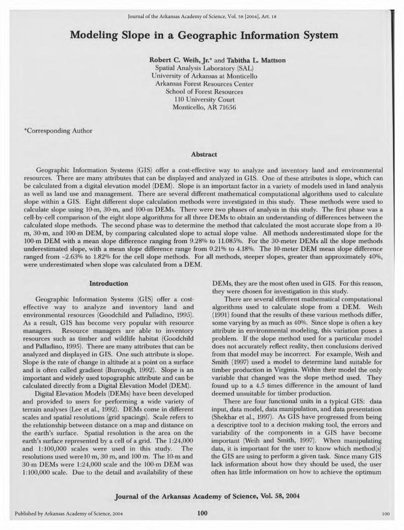
MilesFig. 1. Location of measured points in the study area

results (Burrough, 1992). Unfortunately, the method used todetermine slope is rarely specified in detail by the GISsoftware vendor. The practitioner may therefore be using amethod to calculate slope from a DEM that is not optimalgiven his/her objectives. Also, GIS practitioners are not

always aware of the effects of different methods on theirresults. Therefore, users should become aware of the typesof errors that might exist inany spatial database.

Methods

The study area, approximately 70 square kilometers insize, was located in the Ouachita National Forest inGarlandand Saline counties in central Arkansas. Fig. 1 shows thelocations of the 1,200 points measured inthis study. At eachpoint, slope and latitude/longitude coordinates wererecorded. Point slope measurements were takenapproximately every 100 m along a north-south transect.

Data collectors paced themselves to approximate thisdistance. The slope measurements (percent) were madeusing a Suunto clinometer. On flat terrain, the eye level ofthe data collector was marked on a pole. At each datacollection point, the data collector placed the pole 10 feet

away, based on the maximum slope, and took the upslopeand downslope measurements by aiming the clinometer at

the predetermined eye level. The average of these twoslope measurements was recorded as the slope for thatpoint.

The latitude/longitude coordinates were collected with8 channel handheld GPS receivers. The receivers collected120 positions, meaning they collected one position (latitude,longitude, and elevation) per second for 120 seconds. Therecorded position was the average of these 120 positions,thereby providing a more accurate position. Using PC-GPS" (2.5 and 3.6) software, the GPS data weredifferentially corrected. There were 1130 points that couldbe used in this study after differential correction. Some datawere lost due to the inability to differentially correct them.The total number of points used in the analysis variedbetween the DEMs. This was due to the varying cell size ofthe respective DEMs. The data were examined for eachDEM to verify that only one collection point was within asingle cell. As a result, the total number of points availableafter differential correction for the 10-m, 30-m, and 100-mDEMs were 1125, 1113, and 995 points, respectively.

In this study, raster DEMs were used with square cells.


101


http://scholarworks.uark.edu/jaas/vol58/iss1/18

Modeling Slope ina Geographic Information System

102

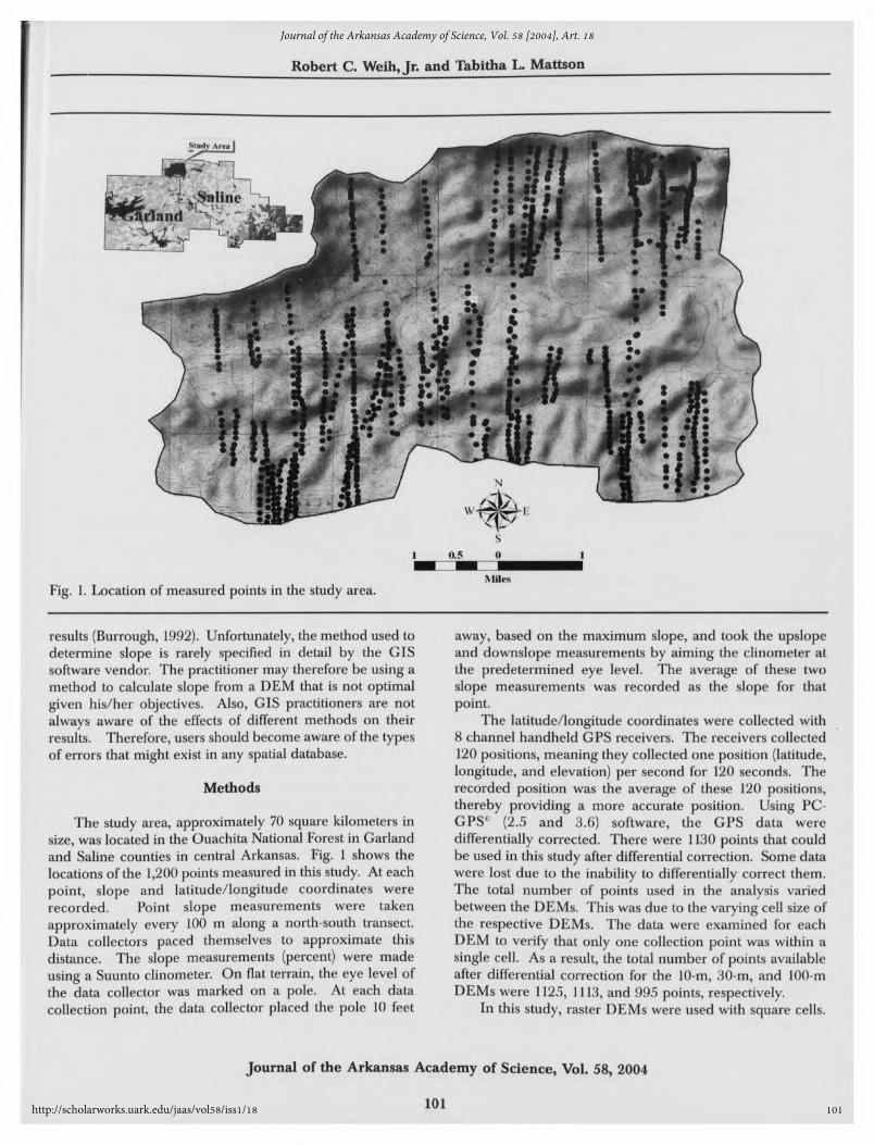
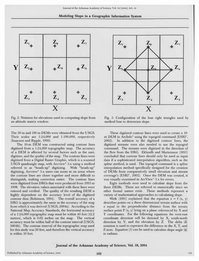
XFig. 2. Notation for elevations used incomputing slope froman altitude matrix window.

Fig. 3. Configuration of the four right triangles used bymethod four to determine slope.

The 30-m and 100-m DEMs were obtained from the USGS.Their scales are 1:24,000 and 1:100,000, respectively(Isaacson and Ripple, 1990).

The 10-m DEM was constructed using contour linesdigitized from a 1:24,000 topographic map. The accuracyof a DEM is affected by several factors such as the user,digitizer, and the quality of the map. The contour lines weredigitized from a Digital Raster Graphic, which is a scannedJSGS quadrangle map, with Arcview" 3.x using a method

referred to as "heads-up" digitizing. With "heads-up"digitizing, Arcview" 3.x users can zoom in on areas wherethe contour lines are closer together and more difficult to

distinguish, making correction easier. The contour lineswere digitized from DRGs that were produced from 1995 to

1998. The elevation values associated with these lines wereentered and verified. The quality of the resulting DEM islighly dependent on the accuracy level of the digitizedcontour data (Robinson, 1994). The overall accuracy of a)RG is approximately the same as the accuracy of the maprom which itwas derived (USGS, 2004a). According to theNational Map Accuracy Standards, the horizontal accuracyof a 1:24,000 topographic map must be within 40 feet (12.2meters), which is 0.02 inches on the map. The verticalaccuracy must be withinhalf of the contour interval (USGS,2004b). The contour interval of the topographic map usedor this study was 20 feet, and therefore the vertical accuracys within 10 feet.

These digitized contour lines were used to create a 10-m DEM in Arclnfo" using the topogrid command (ESRF,2002). In addition to the digitized contour lines, thedigitized streams were also needed to use the topogridcommand. The streams were digitized in the direction ofthe flow from the DRG. Eklundh and Martensson (1995)concluded that contour lines should only be used as inputdata if a sophisticated interpolation algorithm, such as thespline method, is used. The topogrid command is a splineinterpolation method specifically designed for the creationof DEMs from comparatively small elevation and streamcoverage's (ESRF ,2002). Once the DEM was created, itwas visually examined in ArcView" 3.x for errors.

Eight methods were used to calculate slope from thethree DEMs. These are referred to numerically since noother formal names exist. These methods represent avariety of mathematical approaches to calculating slope.

Weih (1991) explained that the equation z = f (x, y)describes points on a three dimensional terrain surface withz equal to the perpendicular distance from the terrainsurface point P (x, y) lyingon a plane referenced by X andY coordinates. For the following equations the west-east

coordinate direction will be denoted by X, south-northdirection by Y, and the elevation by Z. The delta (5)notation is used to represent the difference in the X,Y,andZ-axes. Equation (1) can be used to calculate slope angle ((())inradians.


102



Robert C. Weih, Jr. and Tabitha L.Mattson

103

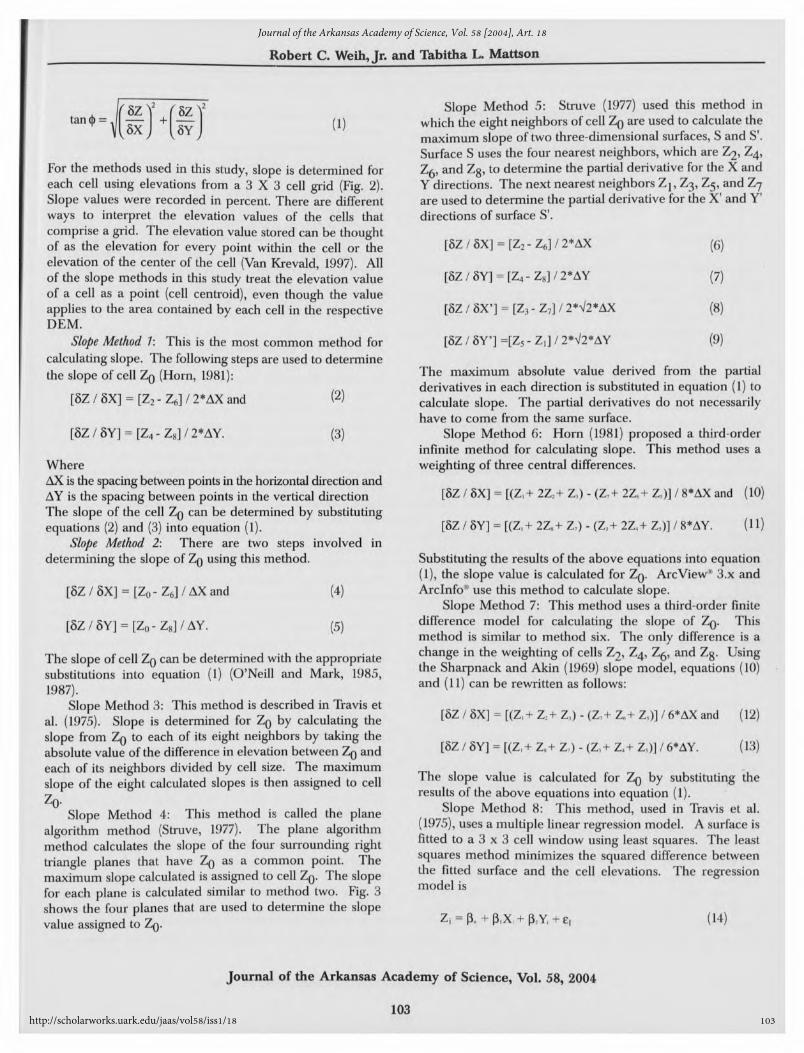
-liHU (1)

For the methods used in this study, slope is determined foreach cell using elevations from a 3 X 3 cell grid (Fig. 2).Slope values were recorded in percent. There are differentways to interpret the elevation values of the cells thatcomprise a grid. The elevation value stored can be thoughtof as the elevation for every point within the cell or theelevation of the center of the cell (Van Krevald, 1997). Allof the slope methods in this study treat the elevation valueof a cell as a point (cell centroid), even though the valueapplies to the area contained by each cell in the respectiveDEM.

Slope Method V. This is the most common method forcalculating slope. The following steps are used to determinethe slope of cell Zq (Horn, 1981):

[8Z / 8X]= [Z2-

Z6]/ 2*AXand (2)

[5Z/5Y]= [Z4 -Z8]/2*AY. (3)

WhereAXis the spacing between points in the horizontal direction andAY is the spacing between points in the vertical directionThe slope of the cell Zq can be determined by substitutingequations (2) and (3) into equation (1).

Slope Method 2: There are two steps involved indetermining the slope of Zq using this method.

(4)[8Z/5X]= [Z0 -Z6]/AXand

[8Z/5Y]= [Z0 -Z8]/AY. (5)

The slope of cell Zq can be determined with the appropriatesubstitutions into equation (1) (O'Neill and Mark, 1985,1987).

Slope Method 3: This method is described in Travis et

al. (1975). Slope is determined for Zq by calculating theslope from Zq to each of its eight neighbors by taking theabsolute value of the difference inelevation between Zq andeach of its neighbors divided by cell size. The maximumslope of the eight calculated slopes is then assigned to cellZq.

Slope Method 4: This method is called the planealgorithm method (Struve, 1977). The plane algorithmmethod calculates the slope of the four surrounding righttriangle planes that have Zq as a common point. Themaximum slope calculated is assigned to cell Zq. The slopefor each plane is calculated similar to method two. Fig. 3shows the four planes that are used to determine the slopevalue assigned to Zq.

Slope Method 5: Struve (1977) used this method in

which the eight neighbors of cell Zq are used to calculate themaximum slope of two three-dimensional surfaces, S and S'.Surface S uses the four nearest neighbors, which are Z2, Z4,Z5,and Zg, to determine the partial derivative for the XandYdirections. The next nearest neighbors Zj, Z3, Z5,and Z7are used to determine the partial derivative for the X'and Y'directions of surface S1.

[5Z/5X] =[Z2 -Z6]/2*AX (6)

(7)[5Z/5Y]=[Z4 -Z8]/2*AY

[5Z / 6X']= [Z3-

Z7] / 2*V2*AX (K)

[5Z /8Y']=[Z3- Z,] / 2*V2*AY (9)

The maximum absolute value derived from the partialderivatives ineach direction is substituted in equation (1) tocalculate slope. The partial derivatives do not necessarilyhave to come from the same surface.

Slope Method 6: Horn (1981) proposed a third-orderinfinite method for calculating slope. This method uses aweighting of three central differences.

[5Z / 8X]-

[(Z,+ 2Z2+ Z,) - (Z7

+ 2Z,+ Z,)] / 8*AXand (10)

[8Z / 5Y] =[(Z,+ 2ZS+ Z7)

-(Z.,+ 2Z4

+Z,)] / 8*AY. (11)

Substituting the results of the above equations intoequation(1), the slope value is calculated for Zq. ArcView" 3.x andArclnfo* use this method to calculate slope.

Slope Method 7: This method uses a third-order finitedifference model for calculating the slope of Zq. Thismethod is similar to method six. The only difference is achange in the weighting of cells Z2, Z4, Zg, and Zg. Usingthe Sharpnack and Akin (1969) slope model, equations (10)and (11) can be rewritten as follows:

[5Z / 8X] = [(Z,+Z2+ Z,) - (Z7

+ Z,+ Z,)] / 6*AXand (12)

(13)[8Z / 8Y]-

[(Z,+ Z»+Z,)-

(Z,+Z4+Z,)] / 6*AY.

The slope value is calculated for Zq by substituting theresults of the above equations into equation (1).

Slope Method 8: This method, used in Travis et al.(1975), uses a multiple linear regression model. Asurface isfitted to a 3 x 3 cell window using least squares. The leastsquares method minimizes the squared difference betweenthe fitted surface and the cell elevations. The regressionmodel is

(14)Zj=p,, +(3,X,+ (32Y,+e,


103




104

Assuming that elis approximately uncorrelated withX andY, the partial derivatives withrespect to X and Y are shownin equations (15) and (16). Substituting equations (15) and(16) into equation (1), the slope value for cell Zq can beobtained.

Substituting [(3E(Z) /dX] =p, for (6Z / 8X) (15)

Substituting [(3E(Z) / 3Y] =p: for (5Z / 5Y) (16)

This method uses all nine elevation values to fitthe surfaceand estimate the slope of cell Zq.

In order to calculate slope using these eight methods,C++ programming was used. ArcView® 3.x Spatial Analysthas a C programming application program interface (API).This API is a grid data set input/output library that allowsthe user to read and write data to and from ESRI grids(ESRI" 1, 1999). These grid data sets were then viewed andanalyzed inArcView® 3.x.

There were two phases of analysis in this study. Thefirst phase was a cell-by-cell comparison of all three DEMsto determine if there was a relationship between thecalculated slope values for the eight different calculationmethods. The second phase was to determine the methodthat calculated the most accurate slope from a 10-m, 30-m,and 100-m DEM by comparison with field slopemeasurements.

A two-sided paired t-test was performed using thestatistical program SAS

'"'to determine ifthe mean difference

between the calculated and measured slopes for a particularDEM was statistically significant (Ho: jnd

=0 and H,: u\d*0,

where |Lid= the mean difference between the measured and

calculated slope). An alpha (a) level of 0.05 was used for thistest. The eight slope methods tested in phase one weretested inphase two.

Results and Discussion

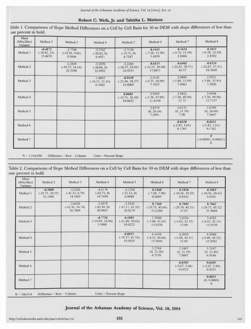
Phase One.- The first phase was a cell-by-cellcomparison of all three DEMs to determine if there was arelationship between the calculated slope values for theeight different calculation methods. For the 10-m, 30-m,and 100-m DEMs 1,116,896, 146,914 and 11,645 cells were

compared, respectively. Allthe slope methods were foundto be statistically different. These results could be due to thelarge sample size. For this reason, it is more useful to

compare the methods using mean differences and variances.The absolute differences are used for comparison with anegative number showing overestimation and a positivenumber showing underestimation.

Table 1 shows the slope method differences for the 10-m DEM. For the 10-m DEM, twelve of the slope methodcomparisons, 1-2, 1-6, 1-7, 1-8, 2-6, 2-7, 2-8, 3-5, 4-5, 6-7, 6-8, and 7-8, had a mean difference of less than +/- one

percent. For practical applications, these methods can beconsidered the same.

Table 2 shows the slope method differences for the 30-m DEM. For this DEM, thirteen of the comparisons, 1-2, 1-6, 1-7, 1-8, 2-6, 2-7, 2-8, 3-4, 3-5, 4-5, 6-7, 6-8, and 7-8, had amean difference of less than +/- one percent. Twelve of thecomparisons were the same as found using the 10-m DEM.As with the 10-m DEM, these methods can be consideredthe same for most applications. Overall, for the 30-m DEM,methods 7 and 8 were the most similar and methods 4 and8 witha mean difference of 4.2040% were the least similar.

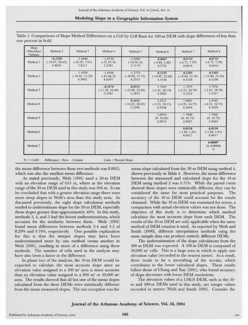
Table 3 shows the slope method differences for the 100-m DEM. A mean difference of less than +/- one percentwas found for the same thirteen comparisons as with the 30-m DEM. Overall, for the 100-m DEM,methods 7 and 8were the most similar and methods 4 and 8 with a meandifference of 1.9542% were the least similar.

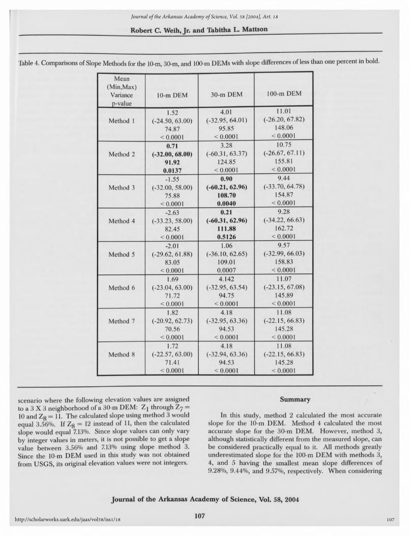
Phase Two.~The second phase was to determine themethod that calculated the most accurate slope from a 10-m,30-m, and 100-m DEM by comparison with field slopemeasurements. A paired t-test (a = 0.05) was used to

determine ifthe mean difference between the measured andcalculated slopes was statistically significant. The results areshown in Table 4. For the 10-m DEM,all of the methodswere found to be statistically different. Method 2, with amean difference of 0.71% and a p-value of 0.0137 was theleast different. For the 30-m DEM, the mean slopecalculated using method 4 with a p-value of 0.5126 was notstatistically different from the mean measured slope (Table4). Allthe other methods had p-values from < 0.0001 to

0.0157. The calculated slopes using method 3 with a meandifference of 0.90% is for most practical purposes, the sameas the measured slope. For the 100-m DEM,all the methodsreturned p-values of< 0.0001. A comparison of the meandifferences in Table 4, which ranged from 9.28% to 11.08%,shows an underestimation of slope using all eight methods.For all the methods, slopes above approximately 40% werealways underestimated. This is illustrated inFig. 4 for slopeMethod 1 for the 10-m and 30-m DEMs.

The results of the cell-by-cell comparison of this studydiffered from those found by Weih (1991). Weih performeda cell-by-cell comparison of a 30-m DEM of Wise and LeeCounties in southwestern Virginia. The DEM elevationrange for the Weih (1991) study was from 424-1079 m, adifference of 655 m. The elevation range of the 30-m DEMused in this study was 211-577 m, a difference of 366 m.Also, there were half as many cells used in the cell-by-cellcomparison in Weih's study, 77,855 as opposed to 146,914.He found less than +/-one percent difference between slopemethods 1-6, 1-7, 1-8, 6-7, 6-8, and 7-8. The results of thisstudy show a less than +/- one percent difference betweenslope methods 1-2, 1-6, 1-7, 1-8, 2-6, 2-7, 2-8, 3-4, 3-5, 4-5, 6-7, 6-8, and 7-8. Weih (1991) found the smallest meandifference, 0.00007, between methods 7 and 8. Inthis study,

Journal of the Arkansas Academy of Science, Vol.58, 2004

104



Robert C. Weih,Jr. and Tabitha L.Mattson

105

rable 1. Comparisons of Slope Method Differences on a Cell by Cell Basis for 10-m DEM with slope differences of less thane percent in bold.

Mean(Min,Max) Method 2 Method 3 Method 4 Method 5 Method 6 Method 7 Method 8

Variance,__^^^^^^^

__ __—.^_^^^^__

-0.4872 -2.7700 -3 7742 -3.7138 0.1441 0.1616 0.1651Method 1 (-38.82,25) (-32.93,9.05) (-38 82 0) (-19.71,0) (-7.28,11.99) (-9.70,15.59) (-9.70,15.59)

15.4479 8.5666 9.4921 8.7247 1.6058 2.8406 2.8382

-2.2828 -3 2870 -3.2266 0.6313 0.6402 0.6524Method2 (-45.57,14.14) (-5000 0) (-30.37,29.93) (-23.25,38.68) (-22.67,38.71) (-22.67,37.31)

22.3280 22.0992 24.9513 17.0471 18.37 18.2649~

-l 0043 -0.9438 2.9141 2.9095 2.9351Method 3 (-16 57 2121) (-22.46,28.27) (-5.37,30.99) (-5.88,33.99) (-5.88,32.93)

6.7685 15.6069 7.1025 7.4462 7.2806

0.0604 3.9183 3.9412 3.9394Method 4 (-19.71,36.30) (-5.38,47.05) (-7.20,49.50) (-7.20,49.50)

19.0652 11.4194 12.72 12.7127

3.8579 4.0135 3.8789Method 5 (0,20.34) (0,21.59) (0,20.68)

7.2891 7.90 7.5667

ftft?/0 0.0211Method 6 (-2.43,3.61) (-2.43,3.61)

0. 1765 0. 1762-

Method 7 (-0.00001,0.00001)0

me

N=1,116,896 Difference =Row-

Column Units = Percent Slope

Table 2. Comparisons of Slope Method Differences on a Cell by Cell Basis for 30-m DEM with slope differences of less than;percent in bold.

Mean(Min,Max) Method 2 Method 3 Method 4 Method 5 Method 6 Method 7 Methods

Variance__-

_^_^^^_____^_^^^^_ ______^^___

-0.5800 -3.2420 -4.0178 -3.1324 0.1460 0.1836 0.1863Method 1 (-42.71,30.55) (-41.33,6.79) (-42.71,0) (-21.14,0) (-7.69,7.98) (-10.36,10.43) (-10.36,10.43)

21.1880 14.1043 14.7450 6.9488 0.4685 0.8343 0.8301

-2.6620 -3.4378 -2.5525 0. 7260 ft7604 ft7662Method2 (-62.45,16.74) (-62.49,0) (-47.11,41.35) (-29.75,45.66) (-29.74,45.31) (-29.73,45.32)

30.7894 30.9947 28.8279 21.6280 21.87 21.9688

-ft7758 0.1095 3.3880 3.4226 3.4282Method 3 (-19.69,18.96) (-21.49,39.02) (-3.80,41.65) (-4.03,42.33) (-4.02,42.33)

3.1088 19.0223 13.8338 13.89 13.9330

0.8853 4.1638 4.2036 4.2040Method 4 (-18.27,41.35) (-4.33,45.66) (-5.88,45.31) (-5.88,45.32)

19.5035 15.5009 15.88 15.9501

3.2784 3.3407 3.3187~

Method 5 (0, 21.20) (0, 2 1.39) (0, 21.40)6.7536 7.0007 6.9186

0.0385 0.0403Method 6 (-2.67, 2.46) (-2.67, 2.46)

0.0523 0.0521

0.0015Method 7 (0, 0.0069)

0

N = 146,914 Difference = Row-

Column Units =Percent Slope


105




106

Table 3. Comparisons of Slope Method Differences on a Cell by CellBasis for 100-m DEM with slope differences of less thanone percent inbold.

Mean(Min,Max) Method 2 Method 3 Method 4 Method 5 Method 6 Method 7 Method 8

Variance-0.2550 -1.6840 -1.8716 -1.6305 0.0605 0.0734 0.0735

Method 1 (-19.87,20.62) (-26.39,7.91) (-32.33,0) (-14.59,0) (-4.88,5.48) (-6.73,7.29) (-6.73,7.29)5.9034 5.8217 5.2281 2.7179 0.3722 0.6616 0.6616

-1.4290 -1.6166 -1.3755 0.3155 0.3285 0.3285Method 2 (-39.45,11.29) (-41.64,0) (-30.98,17.73) (-19.95,22.08) (-19.80,23.38) (-19.80,23.39)

9.5993 8.6397 8.2515 6.3146 6.6104 6.6104

-0.1876 0.0535 1.7445 1.7575 1.7576Method 3 (-11.29,16.69) (-15.98,22.89) (-3.41,28.19) (-2.52,28.79) (-2.52,28.79)

2.2345 5.3833 5.3685 5.3516 5.3517

0.2411 1.9321 1.945 1 1.9542Method 4 (-12.63,28.83) (-3.23,34.13) (-4.53,34.73) (-4.53,34.73)

5.2296 6.0348 6.4438 6.4439

1.6910 1.7040 1.7040Method 5 (0,16.02) (0,16.72) (0,16.72)

2.6916 2.8423 2.8425

0.0130 0.0130Method6 (-1.84,1.81) (-1.84,1.81)

0.0417 0.0417

0.00007Method 7 (0, 0.0004)

0

N=1 1,645 Difference =Row-

Column Units = Percent Slope

the mean difference between these twomethods was 0.0015,which was also the smallest mean difference.

mean slope calculated from the 30-m DEMusing method 4,shown previously in Table 4. However, the mean differencebetween the measured and calculated slope for the 10-mDEM using method 2 was 0.71%. While the paired t-tests

showed these slopes were statistically different, they can beconsidered the same for most practical purposes. Theaccuracy of the 10-m DEM could account for the resultsobtained. While the 10-m DEM was examined for errors, acomparison with actual elevation values was not done. Theobjective of this study is to determine which methodcalculates the most accurate slope from each DEM. Theresults of the 10-m DEMare only applicable when the samemethod of DEMcreation is used. As reported by Weih andSmith (1990), different interpolation methods using thesame sample data can produce entirely different DEMs.

As stated previously, Weih (1991) used a 30-m DEMwith an elevation range of 655 m, where as the elevationrange of the 30-m DEMused in this study was 366 m. Itcanbe concluded that with a greater elevation range there weremore steep slopes in Weih's area than this study area. Asdiscussed previously, the eight slope calculation methodstended to underestimate slope for the 30-m DEM,especiallythose slopes greater than approximately 40%. In this study,methods 3, 4, and 5 had the fewest underestimations, whichaccounts for the similarity between them. Weih (1991)found mean differences between methods 3-4 and 3-5 of8.29% and 9.74%, respectively. One possible explanationfor this is that the steeper slopes may have beenunderestimated more by one method versus another inWeih (1991), resulting in more of a difference using thesemethods. The number of cells used in the analysis mayhave also been a factor in the difference.

The underestimation of the slope calculations from the100-m DEM was expected. A 100-m DEM is composed of10,000 m2 cells. This is a large area in which to apply oneelevation value (recorded to the nearest meter). As a result,there tends to be a smoothing of the terrain, whichcontributes to the lower calculated slopes. These resultsfollow those of Chang and Tsai (1991), who found accuracyof slope decreases with lower DEMresolutions.

Inphase two of the analysis, the 10-m DEM would beexpected to calculate the most accurate slope since anelevation value assigned to a 100 m2 area is more accurate

than an elevation value assigned to a 900 m^ or 10,000 nr'area. The results showed that all but one of the mean slopescalculated from the three DEMs were statistically differentfrom the mean measured slopes. The one exception was the

The elevation values of a USGS DEM, such as the 30-m and 100-m DEMs used in this study, are integer valuesrecorded in meters (Weih and Smith 1990). Consider the

Journal of the Arkansas Academy of Science, Vol.58, 2004

106



Robert C. Weih,Jr. and Tabitha L.Mattson

107

Table 4. Comparisons ofSlope Methods for the 10-m, 30-m, and 100-m DEMs withslope differences of less than one percent inbold.

Mean(Min,Max)

Variance 10-m DEM 30-m DEM 100-m DEM

p-value

1.52 4.01 11.01Method 1 (-24.50,63.00) (-32.95,64.01) (-26.20,67.82)

74.87 95.85 148.06< 0.0001 < 0.0001 < 0-0001

0.71 3.28 10.75

Method 2 (-32.00, 68.00) (-60.3 1,63.37) (-26.67, 67. 1 1)

91.92 124.85 155.810.0137 < 0.0001 < 0.0001

-1.55 0.90 9.44

Method 3 (-32.00, 58.00) (-60.21, 62.96) (-33.70, 64.78)

75.88 108.70 154.87< 0.0001 0.0040 < 0.0001

-2.63 0.21 9.28

Method 4 (-33.23,58.00) (-60.31,62.96) (-34.22,66.63)

82.45 111.88 162.72< 0.0001 0.5126 < 0.0001

-2.01 1.06 9.57

Method 5 (-29.62,61.88) (-36.10,62.65) (-32.99,66.03)83.05 109.01 158.83

< 0.0001 0.0007 < 0.0001

1.69 4.142 11.07Method 6 (-23.04,63.00) (-32.95,63.54) (-23.15,67.08)

71.72 94.75 145.89< 0.0001 < 0.0001 < 0.0001

1.82 4.18 11.08Method 7 (-20.92,62.73) (-32.95,63.36) (-22.15,66.83)

70.56 94.53 145.28< 0.0001 < 0.0001 < 0.0001

1.72 4.18 11.08

Method 8 (-22.57,63.00) (-32.94,63.36) (-22.15,66.83)71.41 94.53 145.28

I < 0.0001 | < 0.0001 I < 0.0001

cenario where the following elevation values are assignedo a 3 X3 neighborhood of a 30-m DEM: Zt through Zy=

0 and Zg= 11. The calculated slope using method 3 wouldqual 3.56%. IfZ# = 12 instead of 11, then the calculatedope would equal 7.13%. Since slope values can only vary

jy integer values in meters, it is not possible to get a slopealue between 3.56% and 7.13% using slope method 3.nee the 10-m DEM used in this study was not obtainedom USGS, its original elevation values were not integers.

Summary

In this study, method 2 calculated the most accurateslope for the 10-m DEM. Method 4 calculated the mostaccurate slope for the 30-m DEM. However, method 3,although statistically different from the measured slope, canbe considered practically equal to it. Allmethods greatlyunderestimated slope for the 100-m DEM with methods 3,4, and 5 having the smallest mean slope differences of9.28%, 9.44%, and 9.57%, respectively. When considering


107




108

error, slope values calculated from the 30-m DEM usingmethod 4 were the most accurate. As when error was notconsidered, allmethods greatly underestimated slope for the100-m DEM,but methods 3,4, and 5 had the smallest meandifferences of 8.84%, 8.71%, and 9.03%, respectively. For allmethods, steeper slopes, greater than approximately 40%,were underestimated.

Acknowledgments. —Funds for this research were

provided by the USDA Forest Service, SouthernExperimental Station and the Arkansas Forest ResourcesCenter (AFRC).

Literature Cited

Burrough, P.A. 1992. Development of IntelligentGeographical Information Systems. Int. J. Geog.Inform. Syst. 6:1-11.

Chang, K., and B. Tsai. 1991. The Effect of DEMResolution on Slope and Aspect Mapping.Cartography and Geog. Inform. Syst. 18:69-77.

Eklundh, L., and U. Martensson. 1995. RapidGeneration of Digital Elevation Models fromTopographic Maps. IntJ. Geog. Inform. Syst. 9:329-340.

ESRF. 1999. ArcView"Version 3.2 a Help:Gridio.ESRT . 2002. Arc/Info" Version 8.2 Help:Topogrid.Goodchild, M. R, and S. D. Palladino. 1995.

Geographic Information Systems as a Tool inScience andTechnology Education. Spec. Sci. Techn. 18:278-286.rorn, B. K. P. 1981. HillShading and the ReflectanceMap. Proc. IEEE 69:14-47.

Isaacson, D.L., and W.J. Ripple. 1990. Comparison of7.5-Minute and 1-Degree Digital Elevation Models.Photogram. Engin. Remote Sens. 56:1523 -1527.

Lee, J., P. K. Snyder, and P. F. Fisher. 1992. Modelingthe Effect of Data Errors on Feature Extraction fromDigital Elevation Models. Photogram. Engin. RemoteSens. 58(10): 1461-1467.

O'NeillM.P., and D.M.Mark. 1985. The Use of DigitalElevation Models in Slope Frequency Analysis.Modeling and Simulation: Proceedings of the AnnualPittsburgh Conference. University of Pittsburgh SchoolofEngineering. Instrument Society ofAmerica. 16:311-315.

O'NeillM.P., and D.M.Mark. 1987. On the FrequencyDistribution of Land Slope. Earth Surf. Proc. Landforms12:127-136.

Robinson, G.J. 1994. The Accuracy of Digital ElevationModels Derived From Digitized Contour Data.Photogram. Record 14:805-814.

Sharpnack, D.A., and G. Akin.1969. An Algorithm forComputing Slope and Aspect from Elevations.Photogram. Engin. Remote Sens. 35:247-248.

Shekhar, S., M.Coyle, B. Goyal, D.Liu,and S. Sarkar.1997. Data Models inGeographic Information Systems.Communications of the ACM 40:103-111.

Struve, H. 1977. An Automated Procedure for Slope MapConstruction. Technical Report M-77-3. U.S. ArmyEngineer Waterways Experiment Station. 98 pp.

Travis, M.R., G. H.Eisner, W. D. Iverson, and C. G.Johnson. 1975. VIEWIT:Computation of Seen Areas,Slopes, and Aspect for Land-Use Planning. GeneralTechnical Report PSW-11. U.S. Forest Service. 70 pp.

United States Geological Survey. 2004a. Overview ofthe USGS Digital Raster Graphic (DRG) Program.[http://topomaps.usgs.gov/drg/], 25 March 2004.

United States Geological Survey. 2004b. Map AccuracyStandards. Fact Sheet FS-171-99,[http://mac.usgs.gov/mac/isb/pubs/factsheets/fsl7199.html], 25 March 2004.

Van Krevald, M. 1997. Digital Elevation Models and TINAlgorithms. Lect. Notes Comp. Sci. 1340:37-78.

Weih, Jr., R. C. 1991. Evaluating Methods forCharacterizing Slope Conditions Within Polygons.Unpublished Ph.D. Dissertation. Virginia PolytechnicInstitute and State University, VA.pp 231

Weih, Jr., R. C, and J. L.Smith. 1990. Characteristicsand Limitations of USGS Digital Elevation Models.Proc. 1990 Landuse Manage. Conf. p. 139-147.

Weih, Jr., R. C, and J. L.Smith. 1997. The Influence ofCell Slope Computation Algorithms on a CommonForest Management Decision. Proceedings of theSeventh International Symposium on Spatial DataHandling: Advances inGIS Research II,p. 857-875.


108



Documents

Modeling Slope in a Geographic Information System