Received: 26 January 2017 Revised: 3 November 2017 Accepted: 3 November 2017

DOI: 10.1002/eqe.3007

R E S E A R C H A R T I C L E

Modeling spatially correlated spectral accelerations atmultiple periods using principal component analysisand geostatistics

Maryia Markhvida Luis Ceferino Jack W. Baker

Department of Civil and EnvironmentalEngineering, Stanford University,Stanford, CA 94305-4020, U.S.A.

CorrespondenceMaryia Markhvida, Department of Civiland Environmental Engineering, StanfordUniversity, Stanford, CA, 94305-4020,U.S.A.Email: markhvid@stanford.edu

Funding informationNational Science Foundation,Grant/Award Number: CMMI 0952402

Summary

Regional seismic risk assessments and quantification of portfolio losses oftenrequire simulation of spatially distributed ground motions at multiple intensitymeasures. For a given earthquake, distributed ground motions are character-ized by spatial correlation and correlation between different intensity measures,known as cross-correlation. This study proposes a new spatial cross-correlationmodel for within-event spectral acceleration residuals that uses a combinationof principal component analysis (PCA) and geostatistics. Records from 45 earth-quakes are used to investigate earthquake-to-earthquake trends in applicationof PCA to spectral acceleration residuals. Based on the findings, PCA is used todetermine coefficients that linearly transform cross-correlated residuals to inde-pendent principal components. Nested semivariogram models are then fit toempirical semivariograms to quantify the spatial correlation of principal compo-nents. The resultant PCA spatial cross-correlation model is shown to be accurateand computationally efficient. A step-by-step procedure and an example arepresented to illustrate the use of the predictive model for rapid simulation ofspatially cross-correlated spectral accelerations at multiple periods.

KEYWORDS

cross-correlation, principal component analysis, spatial correlation, spectral accelerations, seismicrisk

1 INTRODUCTION

Assessment of earthquake risk at a community level requires proper quantification of spatially distributed groundmotions. Empirical ground motion models consider only the marginal probability distribution of ground motion inten-sity for an earthquake scenario.1-5 However, for a risk analysis at a regional level or for a portfolio of assets, one needs toestimate ground motion intensities over the entire area of interest.

In general, ground motion models quantify ground motion at a particular site by predicting the median intensity mea-sure (IM) and adding within- and between-event residuals (see Equation 1 below). Within-event residuals quantify IMvariability from location-to-location for one earthquake event, whereas between-event residuals quantify variability fromearthquake-to-earthquake that is seen at all locations for a given event. The within-event residuals exhibit spatial corre-lation and correlation between IMs (ie, cross-correlation), and the between-event residuals exhibit cross-correlation.6-9

A number of studies have proposed models for quantifying the spatial correlation for a single IM.7,8,10,11 However, when

Earthquake Engng Struct Dyn. 2018;47 1107–1123. wileyonlinelibrary.com/journal/eqe Copyright © 2018 John Wiley & Sons, Ltd. 1107:

1108 MARKHVIDA ET AL.

considering a regional risk assessment or an assessment of a portfolio comprised of heterogeneous structures, there is aneed to use multiple IMs to best quantify earthquake consequences.

A previous study of the effect of spatial cross-correlation on portfolio losses showed that the effect of cross-correlationcan be significant, with greater impact on analysis of the extreme losses.12 In addition, several risk estimation frameworksuse multiple IMs to quantify losses: the FEMA P-58 methodology uses spectral acceleration at the fundamental periodof the building to predict building response13; the Global Earthquake Model has a catalog of fragility curves, comprisedof a variety of structural building typologies that use spectral acceleration at differing periods as input14; and the HAZUSmethodology uses peak ground acceleration for buildings and spectral acceleration at period T = 1.0 second for bridgesto estimate potential damages.15 Therefore, to conduct a comprehensive regional risk analysis, it is necessary to considerboth the spatial dependencies of individual IMs and the spatial dependencies across multiple IMs.

Two approaches have been previously proposed for modeling correlation between multiple sites at different periods: aMarkov-type screening hypothesis7 and a linear model of coregionalization (LMC).16 To obtain reliable regional damage orloss estimates, these models need to produce a large number of IM realizations at a large number of locations. Therefore,for regional analyses, these models can be computationally expensive.

This paper proposes a novel methodology for rapid and accurate modeling of spatial cross-correlation of spectral accel-erations using principal component analysis (PCA). PCA has two key characteristics. First, it allows one to work in anuncorrelated space by applying an orthogonal transformation to a set of correlated variables. Second, it allows for dimen-sionality reduction when simulating data that exhibits high correlation among its variables. For these reasons, PCA is apowerful tool for simulating spectral accelerations at different periods, since they exhibit significant correlation acrossperiods. The research described in this paper applies PCA to a large set of recorded ground motions. Based on the results,an accurate and efficient framework for modeling spatially cross-correlated ground motions at multiple sites is proposed.

2 MODELING SPATIAL VARIABILITY OF CROSS- CORRELATEDVARIABLES

This section describes the procedure for calculating ground motion IM residuals, the methodology for characterizingspatial variability of both univariate and multivariate random functions and different techniques to model the randomfunctions.

2.1 Ground motion residualsCurrent ground motion models assess the marginal probability distribution of earthquake IMs at a single site, given anearthquake scenario and site conditions.1-5 Equation 1 shows a typical ground motion model format at site j due to anevent k:

ln IMk,j = 𝜇lnIM + 𝛿Bk + 𝛿Wk,j, (1)

where ln IMk,j is the logarithm of IM of interest, 𝜇lnIM is the predicted mean of the log IM, 𝛿Bk is the between-event(inter-event) residual for earthquake k with a mean of 0 and standard deviation denoted by 𝜏, and 𝛿Wk,j is the within-event(intra-event) residual for site j and earthquake k with a mean of 0 and standard deviation denoted by 𝜑.

In addition to exhibiting spatial cross-correlation, ground motion residuals have several important characteristics.Empirical studies17 have shown that (1) marginal between- and within-event residuals of spectral accelerations can berepresented by a normal distribution, (2) a set of between- and within-event residuals at different periods at one site canbe represented as a multivariate normal distribution, and (3) the within-event residuals at different sites can be repre-sented by a bivariate normal distribution. Extending these conclusions, we assume that the within-event residuals of thespectral accelerations across different periods at multiple sites can be approximated by a multivariate normal distribu-tion. In this case, only the covariance matrix is needed to construct the multivariate distribution, since the mean of thewithin-event residuals is 0.

2.2 Calculation of within-event residualsThis study used the NGA-West2 empirical ground motion database to select appropriate records.18 The events were filteredusing several criteria. Firstly, only ground motions matching the Chiou and Youngs4 selection criteria were chosen, as this

MARKHVIDA ET AL. 1109

ground motion model was used for the calculation of the residuals. Further, only records having usable residuals for all 19chosen spectral periods ranging from 0.01 to 5 seconds were considered. Lastly, only earthquakes with more records thanthe number of periods, were chosen (to be able to perform PCA for each of the earthquake events). In total, the analysiswas performed on 45 earthquakes having 4910 associated records. The number of records per earthquake ranged from 19to 602. The magnitudes ranged from 3.68 ≤ M ≤ 7.90, where 61% of the records came from events of M ≥ 6.0.

Within-event residuals were calculated using Chiou and Youngs' ground motion model,4 as per Equation 2, where imk,jis the recorded IM from earthquake k at site j, 𝛿bk is the observed between-event residual of earthquake k, and 𝛿wk,j is theresultant within-event residual. The resultant residuals were further normalized by 𝜎k, the sample standard deviation ofthe within-event residuals for earthquake k.

z(x) =𝛿wk,j

𝜎k=

ln(imk,j) − 𝜇lnIM − 𝛿bk

𝜎k(2)

This normalization was performed because the focus of this study is the investigation of spatial cross-correlation ofwithin-event residuals and not the magnitude of variability. For convenience, the normalized residuals for earthquake kand site j will be denoted as z(x), where x is a vector denoting the site's location.

2.3 Spatial variability of univariate joint distributionIn geostatistics, random variables that are distributed over space and exhibit spatial continuity are represented by a ran-dom function, Z(x), where x is the spatial position of the variable. In the case of ground motions, the normalized residualsz(x) for spectral acceleration at a specific natural period of vibration T can be considered samples from a random func-tion Z(x). For a given earthquake, the covariance of a random function Z(x) at 2 different locations x and x′ is given byEquation 3:

Cov(Z(x),Z(x′)) = E[(Z(x) − E [Z(x)])

(Z(x′) − E

[Z(x′)

])], (3)

where Cov() denotes covariance and E[] denotes expectation. Due to the typical lack of repeated observations of Z at agiven location (ie, the lack of multiple ground motions at a given site), the calculation of E [Z(x)] at different points xin space cannot be done, and therefore, it is common to assume second-order stationarity. 19 Second-order stationarityassumes that the first 2 moments of the joint probability distribution are preserved under spatial translation. Under thisassumption the mean E [Z(x)] and the variance Var [Z(x)] have constant values 𝜇Z and 𝜎2

Z, respectively, in all the domain,and the covariance will not depend on specific locations x and x′ but only on the relative separation distance h = x− x′ . Inthe case of ground motions, h is a 2-dimensional vector, since the residuals are observed on a 2-dimensional surface. Pastinvestigations have shown that the covariance between residuals is not dependent on a particular direction, and therefore,the covariance function can be assumed to be isotropic.8,20 Consequently, in this study, the covariances are consideredindependent of the direction, where calculations are based on the magnitude of the separation distance, denoted h.

Using the assumption of stationarity and isotropy, Equation 3 can be rewritten as

Cov(

Z(x),Z(x′))= C(h) = E

[(Z(x) − 𝜇Z) (Z(x + h) − 𝜇Z)

]. (4)

In geostatistics field, the semivariogram function is used to describe spatial dependence.19,21,22 Semivariogram measuresthe spatial decorrelation or dissimilarity, and it is mathematically defined as in Equation 5. The relationship between thesemivariogram and the covariance functions in the case of stationarity is shown in Equation 6.

𝛾(h) = 12

E[(Z(x) − Z(x + h))2] (5)

C(h) = C(0) − 𝛾(h) (6)

The empirical semivariogram can be estimated for a given h from observations using the following expression:

𝛾(h) = 12Nh

Nh∑𝛼=1

[z(x𝛼 + h) − z(x𝛼)

]2, (7)

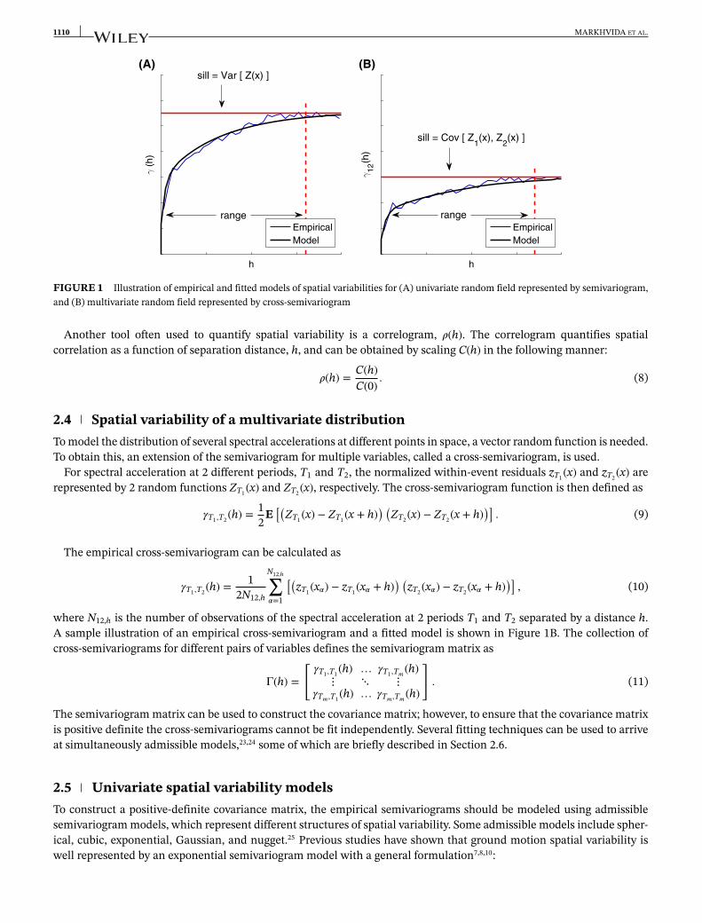
where Nh is the number of observations separated by a distance h. A sample illustration of an empirical semivariogramand a fitted model is shown in Figure 1A. In practice, when the semivariogram is constructed, the set of observations fora given h is chosen with a certain level of tolerance Δ, where the separation distance falls in the interval [h − Δ, h + Δ].

1110 MARKHVIDA ET AL.

h

12(h

)

range

sill = Cov [ Z1(x), Z

2(x) ]

(B)

EmpiricalModel

h

(h)

range

sill = Var [ Z(x) ](A)

EmpiricalModel

FIGURE 1 Illustration of empirical and fitted models of spatial variabilities for (A) univariate random field represented by semivariogram,and (B) multivariate random field represented by cross-semivariogram

Another tool often used to quantify spatial variability is a correlogram, 𝜌(h). The correlogram quantifies spatialcorrelation as a function of separation distance, h, and can be obtained by scaling C(h) in the following manner:

𝜌(h) = C(h)C(0)

. (8)

2.4 Spatial variability of a multivariate distributionTo model the distribution of several spectral accelerations at different points in space, a vector random function is needed.To obtain this, an extension of the semivariogram for multiple variables, called a cross-semivariogram, is used.

For spectral acceleration at 2 different periods, T1 and T2, the normalized within-event residuals zT1 (x) and zT2 (x) arerepresented by 2 random functions ZT1(x) and ZT2(x), respectively. The cross-semivariogram function is then defined as

𝛾T1,T2 (h) =12

E[(

ZT1(x) − ZT1(x + h)) (

ZT2 (x) − ZT2 (x + h))]

. (9)

The empirical cross-semivariogram can be calculated as

𝛾T1,T2 (h) =1

2N12,h

N12,h∑𝛼=1

[(zT1 (x𝛼) − zT1(x𝛼 + h)

) (zT2(x𝛼) − zT2 (x𝛼 + h)

)], (10)

where N12,h is the number of observations of the spectral acceleration at 2 periods T1 and T2 separated by a distance h.A sample illustration of an empirical cross-semivariogram and a fitted model is shown in Figure 1B. The collection ofcross-semivariograms for different pairs of variables defines the semivariogram matrix as

Γ(h) =

[𝛾T1,T1 (h) … 𝛾T1,Tm (h)

⋮ ⋱ ⋮𝛾Tm,T1 (h) … 𝛾Tm,Tm (h)

]. (11)

The semivariogram matrix can be used to construct the covariance matrix; however, to ensure that the covariance matrixis positive definite the cross-semivariograms cannot be fit independently. Several fitting techniques can be used to arriveat simultaneously admissible models,23,24 some of which are briefly described in Section 2.6.

2.5 Univariate spatial variability modelsTo construct a positive-definite covariance matrix, the empirical semivariograms should be modeled using admissiblesemivariogram models, which represent different structures of spatial variability. Some admissible models include spher-ical, cubic, exponential, Gaussian, and nugget.25 Previous studies have shown that ground motion spatial variability iswell represented by an exponential semivariogram model with a general formulation7,8,10:

MARKHVIDA ET AL. 1111

𝛾(h) = S[

1 − exp(−3h

R

)], (12)

where the sill (S) represents the semivariance limit or the overall variance, S = Var[Z(x)] = 𝜎2Z, of the variable. In the case

of the exponential semivariogram, this limit is reached asymptotically. For an exponential model, the practical range (R)is the separation distance at which 95% of the sill value is reached.

A second useful semivariogram model is the nugget model (analogous to white noise), which represents discontinuityat short distances and introduces initial variability. The nugget model has the following formulation:

𝛾(h) ={

0 if h = 0,S if h > 0. (13)

To represent spatial variability in which multiple structures are present, a linear combination of different semivariogrammodels can be used.19 These types of models are referred to as nested semivariogram models.

2.6 Previously proposed multivariate spatial variability modelsThis section describes two existing methods that model cross-correlation among spatially distributed spectral accel-erations. The PCA methodology for modeling multivariate spatial variability used in this study is described inSection 3.

2.6.1 Markov-type screening hypothesis modelOne way to model spatially cross-correlated spectral accelerations at different periods is by using a Markov-type screeninghypothesis, where colocated data z1(x) at location x is assumed to screen the influence of other data points z1(x + h) onrandom secondary variable Z2(x)24:

E[Z2(x)|Z1(x);Z1(x + h)

]= E [Z2(x)|Z1(x)] . (14)

This hypothesis was used in a model proposed by Goda and Hong to model the correlation in spectral accelerations atdifferent periods, denoted by 𝜌𝜀, at a distance h.7 This model has the following formulation:

𝜌𝜀(h,Tn1,Tn2) ≈ 𝜌0(Tn1,Tn2)𝜌𝜀(h,Tmax,Tmax) (15)

where Tmax is the larger of Tn1 and Tn2, 𝜌0 represents the correlation coefficient between the spectral accelerations at agiven location, and 𝜌𝜀(h,Tmax,Tmax) is a univariate correlogram for spectral acceleration at Tmax evaluated at a distance h.

While this model ensures that the resulting covariance matrix is positive definite as long as 𝜌0 and 𝜌𝜀 are admissible,it does not consider the cross-correlation of variables that are not colocated. It has been shown that while this hypoth-esis is a good approximation for periods that are close to one another, it becomes less accurate when the periods differsubstantially.16

2.6.2 Linear model of coregionalizationThe LMC19,23 assumes that the cross-correlated variables are linear combinations of the same underlying structures, sothe semivariogram matrix can be formulated as16

Γ(h) =L∑

l=1Blgl(h), (16)

where the sum is over L cross-semivariograms, Bl are the positive definite coregionalization matrices, and gl(h) are admis-sible semivariogram functions. Loth and Baker16 used LMC to propose a model for simulating spectral accelerations at 6periods: 0.01, 0.1, 0.2, 1, 2, and 5 seconds.

Using the LMC methodology to characterize spatially cross-correlated spectral accelerations at different periodspresents some challenges and complexities, especially as one increases the number of periods to be simulated. One of thesechallenges is to obtain a version of Equation 16 that can accurately represent the large number of cross-semivariogramswhile keeping the B matrices positive definite. For m different periods, the set of parameters that define Equation 16require the fitting of m×(m+1)

2cross-semivariograms.

1112 MARKHVIDA ET AL.

The covariance matrix grows quickly with the addition of extra periods for spectral accelerations. If there are n locationsand m periods to be simulated, the covariance matrix dimensions become (nm) × (nm), which can impose computationalrestrictions for a large number of n or m. This is true for both Markov-type screening and LMC models.

3 PROPOSED PRINCIPAL COMPONENT MODEL FOR GROUND MOTIONS

This section describes how PCA and semivariograms were used to develop a model for spatial variability ofcross-correlated spectral accelerations.

3.1 Principal component analysisPrincipal component analysis performs a linear transformation of the variables of interest to an orthogonal basis, wherethe resulting projections onto the new basis are uncorrelated and are called principal components. The first princi-pal component has the largest variance, the second principal component has the second largest variance constrainedon orthogonality with the previous component, and so on. Principal component analysis yields as many principalcomponents as there are original variables.

There are techniques that can quickly perform PCA and calculate the transformation matrix along with the principalcomponents.26 Equations 17 or 18 define the linear transformation that allows one to pass from the original space (inour case, normalized spectral acceleration residuals at different periods) to a principal component space, where P is anorthogonal linear transformation matrix, Z is the matrix of original data where each row represents different observationsof variables, and Y is a matrix of transformed variables where rows represent different uncorrelated principal components.

PZ = Y (17)

⎡⎢⎢⎢⎣p1,T1 … p1,Tm

⋮ ⋱ ⋮

pm,T1 … pm,Tm

⎤⎥⎥⎥⎦⎡⎢⎢⎢⎣

zT1 (x1) … zT1 (xn)⋮ ⋱ ⋮

zTm(x1) … zTm(xn)

⎤⎥⎥⎥⎦ =⎡⎢⎢⎢⎣

y1(x1) … y1(xn)⋮ ⋱ ⋮

ym(x1) … ym(xn)

⎤⎥⎥⎥⎦ (18)

Analogously the principal components can be transformed back to the original space as follows:

Z = P− 1Y. (19)

Since P is an orthogonal matrix, the following equivalence holds:

Z = PTY. (20)

Equation 21 represents the elements of the principal component i. Since principal components are uncorrelated, the spa-tial variability characterization of Yi can be done independently of any other component Yi′ . Only the spatial correlationamong the elements of Yi in Equation 21 should be considered.

Yi =[

yi(x1) yi(x2) … yi(xn)]

(21)

The fact that the principal components are uncorrelated eliminates the need for cross-semivariograms and allows oneto calculate a semivariogram with Equation 7 for each of the components independently.

By changing the basis, PCA can provide us with the ability to reduce the dimensionality of the problem to a smallernumber of independent dimensions. In the case of ground motions, it would mean that the desired number of spectralaccelerations at different periods can be simulated with a smaller number of variables. To know how many componentswe need to simulate to represent most of the variability in the data set, the variance Var[Yi] of each component can becalculated. The sum of the variances for all the components adds up to the total variance in the dataset, as shown inEquation 22. In practice, it is common to use enough components such that the variance adds up to anywhere from 70%to 95% of the total variance,27,28 as shown in Equation 23 where the 95% threshold was chosen.

Var[Total] =m∑

i=1Var[zTi(x)] =

m∑i=1

Var[Yi] (22)

MARKHVIDA ET AL. 1113

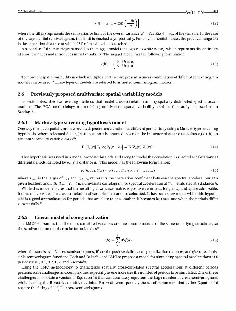
FIGURE 2 Cumulative contribution of each principal component to the explained variance of the variables for individual earthquakeevents (EQ) and pooled records

%𝜎2expl.cum =

∑m95

i=1Var[Yi]

Var[Total]≥ 0.95 (23)

3.2 Principal component coefficientsPrincipal component analysis was performed on each of the 45 considered earthquakes separately using the approachdescribed in Section 3.1, to obtain principal component coefficient vectors. In addition, PCA was performed on the nor-malized residuals when the data from the 45 earthquakes was pooled together. Figure 2 shows the cumulative varianceexplained (%𝜎2

expl.cum) by each of the principal components for single earthquake events, as well as when the records arepooled and analyzed together. When the records are pooled, 5 components explain 95% of the variance. The percent ofexplained variance (%𝜎2

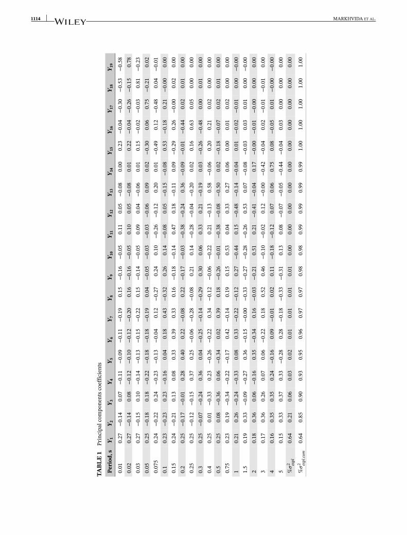
expl) and cumulative percent of explained variance for each of the principal components is sum-marized in Table 1. The evident reduction of observed variables to a smaller set of transformed variables that explainmost of the variance suggests that different spectral accelerations are measuring the same underlying structures. Thisimplies that spectral accelerations for considered periods can be modeled as a linear combination of a reduced numberof variables.

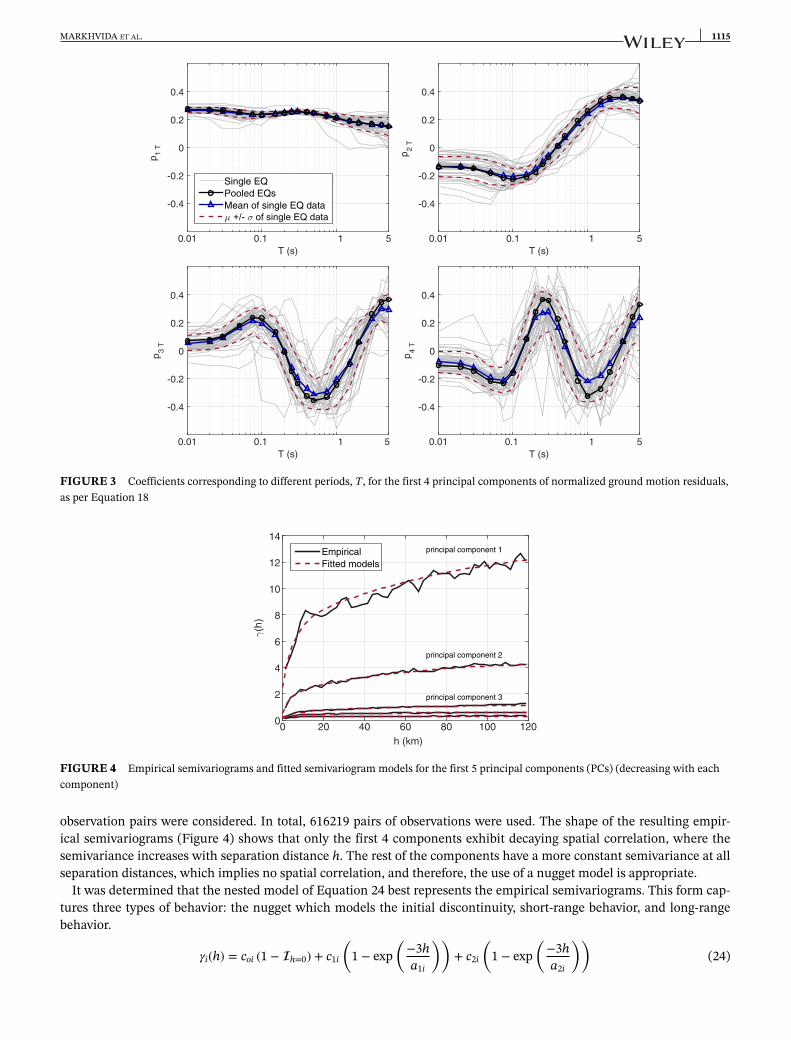
Figure 3 shows the transformation coefficients corresponding to different periods for the 45 single earthquake events.Performing PCA on the 45 events reveals that for each of the principal components, the transformation coefficients followa similar trend across the periods. This is especially evident in principal components 1 and 2, which capture most of thevariables' variance. In addition, the mean of the 45 coefficients for single earthquakes closely resembles the transformationcoefficients obtained when all the records are pooled and analyzed together. To create a single model for spatial variabilityand to ensure that the components remain independent, the coefficients used in the model were obtained by poolingrecords from the 45 earthquakes.

Table 1 summarizes the transformation coefficients obtained for each of the principal components. In the case that aperiod not explicitly considered in the model is required, the coefficient can be linearly interpolated between periods foreach of the principal components. This methodology was verified by adding an extra period, rerunning PCA and modelingsemivariograms in both the principal component and the original spaces. The results of the interpolation and the analysiswith an extra period were practically the same and did not have an effect of the modeling parameters.

3.3 Semivariogram models for principal componentsThe choice of the semivariogram models is dependent on the shape of empirical semivariograms and previous knowledgeabout the random function being modeled. Manual visual fits of the empirical semivariograms were performed, followingcommon practice, since the precise fit of the points is less important than the behavior at short separation distances andconsideration of what happens at large distances.21,29

The empirical semivariograms for each of the principal components were calculated using lag tolerance, Δ = 2.5 km.The semivariograms were constructed using all of the pooled data, where for each earthquake all combinations of

1114 MARKHVIDA ET AL.

TAB

LE1

Prin

cipa

lcom

pone

ntsc

oeffi

cien

ts

Peri

od,s

Y 1Y 2

Y 3Y 4

Y 5Y 6

Y 7Y 8

Y 9Y 1

0Y 1

1Y 1

2Y 1

3Y 1

4Y 1

5Y 1

6Y 1

7Y 1

8Y 1

9

0.01

0.27

−0.

140.

07−

0.11

−0.

09−

0.11

−0.

190.

15−

0.16

−0.

050.

110.

05−

0.08

0.00

0.23

−0.

04−

0.30

−0.

53−

0.58

0.02

0.27

−0.

140.

08−

0.12

−0.

10−

0.12

−0.

200.

16−

0.16

−0.

050.

100.

05−

0.08

0.01

0.22

−0.

04−

0.26

−0.

150.

780.

030.

27−

0.15

0.10

−0.

14−

0.13

−0.

15−

0.22

0.15

−0.

14−

0.05

0.09

0.04

−0.

060.

010.

15−

0.02

−0.

030.

81−

0.23

0.05

0.25

−0.

180.

18−

0.22

−0.

18−

0.18

−0.

190.

04−

0.05

−0.

03−

0.03

−0.

060.

090.

02−

0.30

0.06

0.75

−0.

210.

020.

075

0.24

−0.

220.

24−

0.23

−0.

13−

0.04

0.12

−0.

270.

240.

10−

0.26

−0.

120.

200.

01−

0.49

0.12

−0.

480.

04−

0.01

0.1

0.23

−0.

230.

23−

0.16

0.04

0.18

0.43

−0.

320.

260.

14−

0.08

0.05

−0.

15−

0.08

0.53

−0.

180.

21−

0.00

0.00

0.15

0.24

−0.

210.

130.

080.

330.

390.

330.

16−

0.18

−0.

140.

470.

18−

0.11

0.09

−0.

290.

26−

0.00

0.02

0.00

0.2

0.25

−0.

17−

0.01

0.28

0.40

0.22

−0.

080.

22−

0.17

−0.

03−

0.38

−0.

240.

36−

0.09

−0.

01−

0.44

0.02

0.01

0.00

0.25

0.25

−0.

12−

0.15

0.37

0.25

−0.

06−

0.28

−0.

080.

210.

14−

0.28

−0.

04−

0.20

0.02

0.16

0.63

0.05

0.00

0.00

0.3

0.25

−0.

07−

0.24

0.36

0.04

−0.

25−

0.14

−0.

290.

300.

060.

330.

21−

0.19

0.03

−0.

26−

0.48

0.00

0.01

0.00

0.4

0.25

0.01

−0.

330.

23−

0.26

−0.

220.

34−

0.12

−0.

06−

0.22

0.21

−0.

130.

58−

0.06

0.20

0.21

0.02

0.00

0.00

0.5

0.25

0.08

−0.

360.

06−

0.34

0.02

0.39

0.18

−0.

26−

0.01

−0.

38−

0.08

−0.

500.

02−

0.18

−0.

070.

020.

010.

000.

750.

230.

19−

0.34

−0.

22−

0.17

0.42

−0.

140.

190.

150.

530.

040.

330.

270.

060.

000.

010.

020.

000.

001

0.21

0.26

−0.

24−

0.33

0.08

0.33

−0.

22−

0.12

0.27

−0.

440.

15−

0.48

−0.

14−

0.04

0.01

−0.

02−

0.01

0.00

−0.

001.

50.

190.

33−

0.09

−0.

270.

36−

0.15

−0.

00−

0.33

−0.

27−

0.28

−0.

260.

530.

07−

0.08

−0.

030.

030.

010.

00−

0.00

20.

180.

360.

06−

0.16

0.35

−0.

340.

16−

0.03

−0.

210.

510.

21−

0.41

−0.

040.

17−

0.00

−0.

01−

0.00

0.00

0.00

30.

170.

360.

260.

070.

06−

0.22

0.18

0.52

0.46

−0.

10−

0.02

0.12

−0.

00−

0.42

−0.

040.

02−

0.01

−0.

010.

004

0.16

0.35

0.35

0.24

−0.

160.

09−

0.01

0.02

0.11

−0.

18−

0.12

0.07

0.06

0.75

0.08

−0.

050.

01−

0.00

−0.

005

0.15

0.33

0.37

0.33

−0.

280.

28−

0.18

−0.

33−

0.31

0.13

0.08

−0.

07−

0.05

−0.

44−

0.04

0.03

0.00

0.00

0.00

%𝜎

2 expl

0.64

0.21

0.06

0.03

0.02

0.01

0.01

0.01

0.01

0.00

0.00

0.00

0.00

0.00

0.00

0.00

0.00

0.00

0.00

%𝜎

2 expl.cu

m0.

640.

850.

900.

930.

950.

960.

970.

970.

980.

980.

990.

990.

990.

991.

001.

001.

001.

001.

00

MARKHVIDA ET AL. 1115

T (s)

p 1 T

-0.4

-0.2

0

0.2

0.4

Single EQPooled EQsMean of single EQ data

T (s)

p2

T

-0.4

-0.2

0

0.2

0.4

T (s)

p3

T

-0.4

-0.2

0

0.2

0.4

T (s)

0.01 0.1 1 5 0.01 0.1 1 5

0.01 0.1 1 5 0.01 0.1 1 5

p4

T-0.4

-0.2

0

0.2

0.4

FIGURE 3 Coefficients corresponding to different periods, T, for the first 4 principal components of normalized ground motion residuals,as per Equation 18

h (km)0 20 40 60 80 100 1200

2

4

6

8

10

12

14principal component 1

principal component 2

principal component 3

EmpiricalFitted models

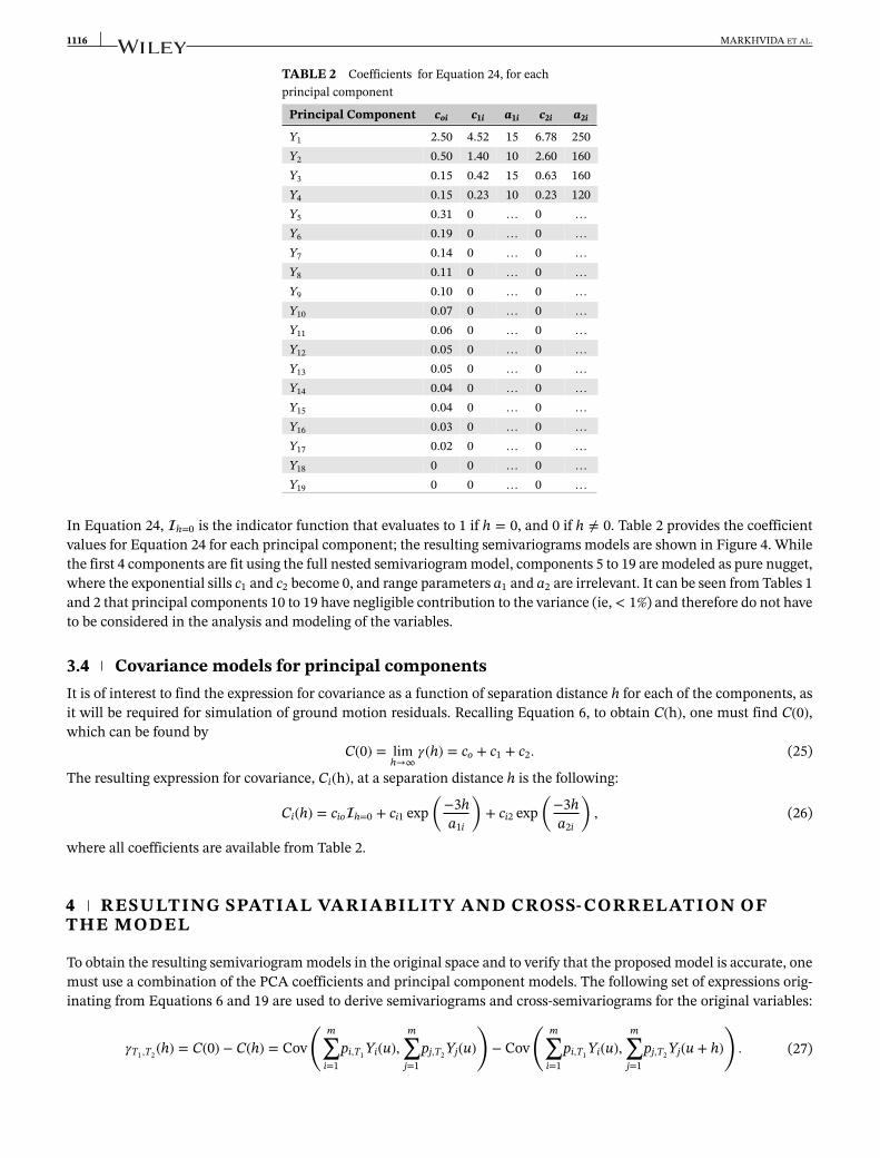
FIGURE 4 Empirical semivariograms and fitted semivariogram models for the first 5 principal components (PCs) (decreasing with eachcomponent)

observation pairs were considered. In total, 616219 pairs of observations were used. The shape of the resulting empir-ical semivariograms (Figure 4) shows that only the first 4 components exhibit decaying spatial correlation, where thesemivariance increases with separation distance h. The rest of the components have a more constant semivariance at allseparation distances, which implies no spatial correlation, and therefore, the use of a nugget model is appropriate.

It was determined that the nested model of Equation 24 best represents the empirical semivariograms. This form cap-tures three types of behavior: the nugget which models the initial discontinuity, short-range behavior, and long-rangebehavior.

𝛾i(h) = coi (1 − h=0) + c1i

(1 − exp

(−3ha1i

))+ c2i

(1 − exp

(−3ha2i

))(24)

1116 MARKHVIDA ET AL.

TABLE 2 Coefficients for Equation 24, for eachprincipal component

Principal Component coi c1i a1i c2i a2i

Y1 2.50 4.52 15 6.78 250Y2 0.50 1.40 10 2.60 160Y3 0.15 0.42 15 0.63 160Y4 0.15 0.23 10 0.23 120Y5 0.31 0 … 0 …Y6 0.19 0 … 0 …Y7 0.14 0 … 0 …Y8 0.11 0 … 0 …Y9 0.10 0 … 0 …Y10 0.07 0 … 0 …Y11 0.06 0 … 0 …Y12 0.05 0 … 0 …Y13 0.05 0 … 0 …Y14 0.04 0 … 0 …Y15 0.04 0 … 0 …Y16 0.03 0 … 0 …Y17 0.02 0 … 0 …Y18 0 0 … 0 …Y19 0 0 … 0 …

In Equation 24, h=0 is the indicator function that evaluates to 1 if h = 0, and 0 if h ≠ 0. Table 2 provides the coefficientvalues for Equation 24 for each principal component; the resulting semivariograms models are shown in Figure 4. Whilethe first 4 components are fit using the full nested semivariogram model, components 5 to 19 are modeled as pure nugget,where the exponential sills c1 and c2 become 0, and range parameters a1 and a2 are irrelevant. It can be seen from Tables 1and 2 that principal components 10 to 19 have negligible contribution to the variance (ie, < 1%) and therefore do not haveto be considered in the analysis and modeling of the variables.

3.4 Covariance models for principal componentsIt is of interest to find the expression for covariance as a function of separation distance h for each of the components, asit will be required for simulation of ground motion residuals. Recalling Equation 6, to obtain C(h), one must find C(0),which can be found by

C(0) = limh→∞

𝛾(h) = co + c1 + c2. (25)

The resulting expression for covariance, Ci(h), at a separation distance h is the following:

Ci(h) = cioh=0 + ci1 exp(−3ha1i

)+ ci2 exp

(−3ha2i

), (26)

where all coefficients are available from Table 2.

4 RESULTING SPATIAL VARIABILITY AND CROSS- CORRELATION OFTHE MODEL

To obtain the resulting semivariogram models in the original space and to verify that the proposed model is accurate, onemust use a combination of the PCA coefficients and principal component models. The following set of expressions orig-inating from Equations 6 and 19 are used to derive semivariograms and cross-semivariograms for the original variables:

𝛾T1,T2 (h) = C(0) − C(h) = Cov

( m∑i=1

pi,T1 Yi(u),m∑

j=1pj,T2 Yj(u)

)− Cov

( m∑i=1

pi,T1 Yi(u),m∑

j=1pj,T2 Yj(u + h)

). (27)

MARKHVIDA ET AL. 1117

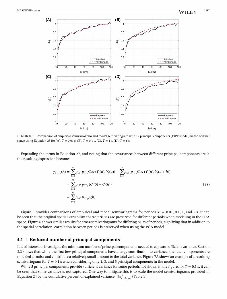
FIGURE 5 Comparison of empirical semivariogram and model semivariogram with 19 principal components (19PC model) in the originalspace using Equation 28 for (A), T = 0.01 s, (B), T = 0.1 s, (C), T = 1 s, (D), T = 5 s

Expanding the terms in Equation 27, and noting that the covariances between different principal components are 0,the resulting expression becomes

𝛾T1,T2(h) =m∑

i=1pi,T1 pi,T2 Cov (Yi(u),Yi(u)) −

m∑i=1

pi,T1 pi,T2 Cov (Yi(u),Yi(u + h))

=m∑

i=1pi,T1 pi,T2 (Ci(0) − Ci(h))

=m∑

i=1pi,T1 pi,T2𝛾i(h).

(28)

Figure 5 provides comparisons of empirical and model semivariograms for periods T = 0.01, 0.1, 1, and 5 s. It canbe seen that the original spatial variability characteristics are preserved for different periods when modeling in the PCAspace. Figure 6 shows similar results for cross-semivariograms for differing pairs of periods, signifying that in addition tothe spatial correlation, correlation between periods is preserved when using the PCA model.

4.1 Reduced number of principal componentsIt is of interest to investigate the minimum number of principal components needed to capture sufficient variance. Section3.3 shows that while the first few principal components have a large contribution to variance, the later components aremodeled as noise and contribute a relatively small amount to the total variance. Figure 7A shows an example of a resultingsemivariogram for T = 0.1 s when considering only 1, 3, and 5 principal components in the model.

While 5 principal components provide sufficient variance for some periods not shown in the figure, for T = 0.1 s, it canbe seen that some variance is not captured. One way to mitigate this is to scale the model semivariograms provided inEquation 24 by the cumulative percent of explained variance, %𝜎2

expl.cum (Table 1).

1118 MARKHVIDA ET AL.

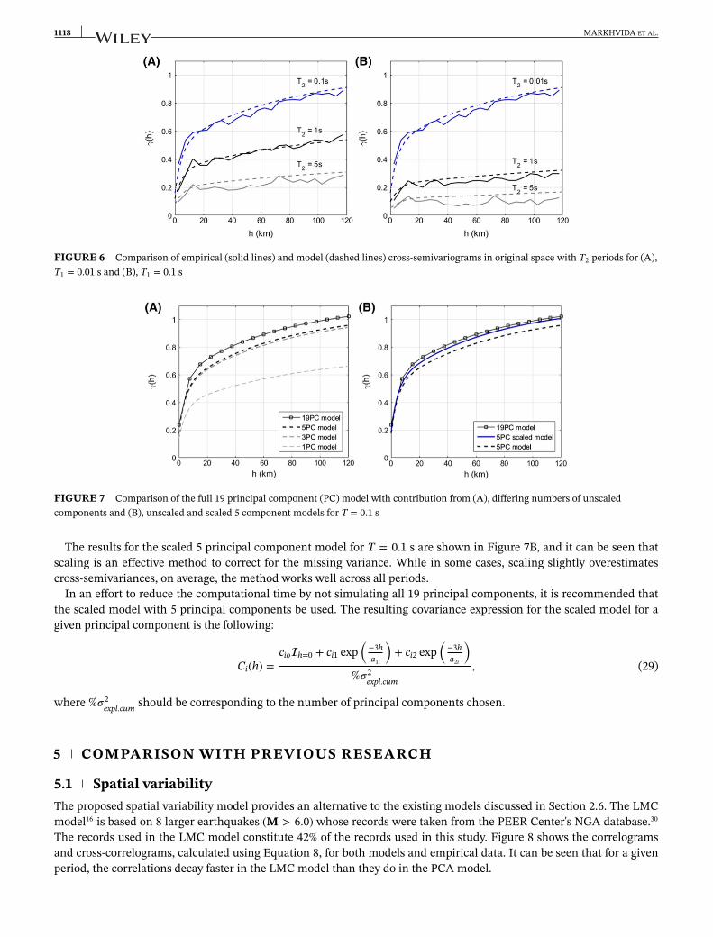
FIGURE 6 Comparison of empirical (solid lines) and model (dashed lines) cross-semivariograms in original space with T2 periods for (A),T1 = 0.01 s and (B), T1 = 0.1 s

FIGURE 7 Comparison of the full 19 principal component (PC) model with contribution from (A), differing numbers of unscaledcomponents and (B), unscaled and scaled 5 component models for T = 0.1 s

The results for the scaled 5 principal component model for T = 0.1 s are shown in Figure 7B, and it can be seen thatscaling is an effective method to correct for the missing variance. While in some cases, scaling slightly overestimatescross-semivariances, on average, the method works well across all periods.

In an effort to reduce the computational time by not simulating all 19 principal components, it is recommended thatthe scaled model with 5 principal components be used. The resulting covariance expression for the scaled model for agiven principal component is the following:

Ci(h) =cioh=0 + ci1 exp

(−3ha1i

)+ ci2 exp

(−3ha2i

)%𝜎2

expl.cum

, (29)

where %𝜎2expl.cum should be corresponding to the number of principal components chosen.

5 COMPARISON WITH PREVIOUS RESEARCH

5.1 Spatial variabilityThe proposed spatial variability model provides an alternative to the existing models discussed in Section 2.6. The LMCmodel16 is based on 8 larger earthquakes (M > 6.0) whose records were taken from the PEER Center's NGA database.30

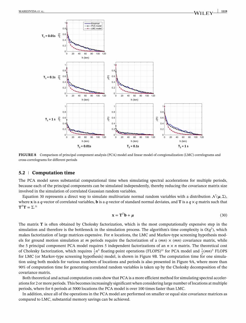
The records used in the LMC model constitute 42% of the records used in this study. Figure 8 shows the correlogramsand cross-correlograms, calculated using Equation 8, for both models and empirical data. It can be seen that for a givenperiod, the correlations decay faster in the LMC model than they do in the PCA model.

MARKHVIDA ET AL. 1119

FIGURE 8 Comparison of principal component analysis (PCA) model and linear model of coregionalization (LMC) correlograms andcross-correlograms for different periods

5.2 Computation timeThe PCA model saves substantial computational time when simulating spectral accelerations for multiple periods,because each of the principal components can be simulated independently, thereby reducing the covariance matrix sizeinvolved in the simulation of correlated Gaussian random variables.

Equation 30 represents a direct way to simulate multivariate normal random variables with a distribution (𝝁,Σ),where x is a q-vector of correlated variables, b is a q-vector of standard normal deviates, and T is a q × q matrix such thatTTT = Σ.31

x = TTb + 𝝁 (30)

The matrix T is often obtained by Cholesky factorization, which is the most computationally expensive step in thesimulation and therefore is the bottleneck in the simulation process. The algorithm's time complexity is O(q3), whichmakes factorization of large matrices expensive. For n locations, the LMC and Markov-type screening hypothesis mod-els for ground motion simulation at m periods require the factorization of a (mn) × (mn) covariance matrix, whilethe 5 principal component PCA model requires 5 independent factorizations of an n × n matrix. The theoretical costof Cholesky factorization, which requires 1

3n3 floating-point operations (FLOPS)32 for PCA model and 1

3(mn)3 FLOPS

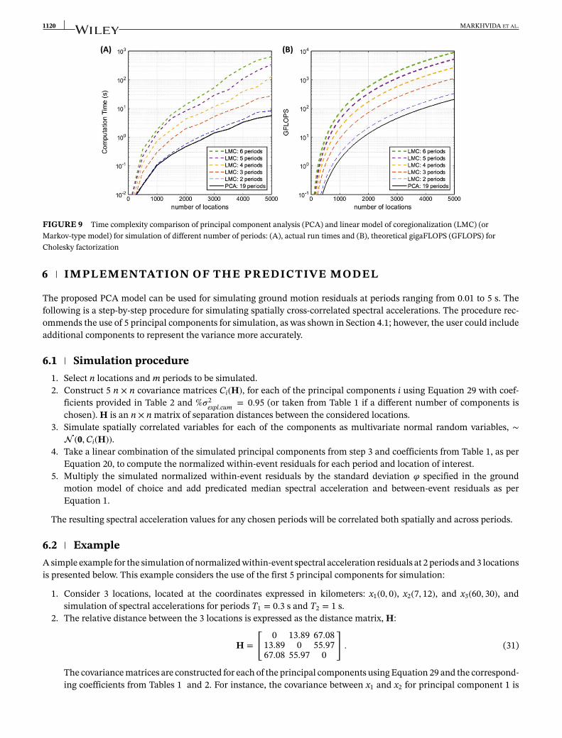
for LMC (or Markov-type screening hypothesis) model, is shown in Figure 9B. The computation time for one simula-tion using both models for various numbers of locations and periods is also presented in Figure 9A, where more than90% of computation time for generating correlated random variables is taken up by the Cholesky decomposition of thecovariance matrix.

Both theoretical and actual computation costs show that PCA is a more efficient method for simulating spectral acceler-ations for 2 or more periods. This becomes increasingly significant when considering large number of locations at multipleperiods, where for 6 periods at 5000 locations the PCA model is over 100 times faster than LMC.

In addition, since all of the operations in the PCA model are performed on smaller or equal size covariance matrices ascompared to LMC, substantial memory savings can be achieved.

1120 MARKHVIDA ET AL.

FIGURE 9 Time complexity comparison of principal component analysis (PCA) and linear model of coregionalization (LMC) (orMarkov-type model) for simulation of different number of periods: (A), actual run times and (B), theoretical gigaFLOPS (GFLOPS) forCholesky factorization

6 IMPLEMENTATION OF THE PREDICTIVE MODEL

The proposed PCA model can be used for simulating ground motion residuals at periods ranging from 0.01 to 5 s. Thefollowing is a step-by-step procedure for simulating spatially cross-correlated spectral accelerations. The procedure rec-ommends the use of 5 principal components for simulation, as was shown in Section 4.1; however, the user could includeadditional components to represent the variance more accurately.

6.1 Simulation procedure1. Select n locations and m periods to be simulated.2. Construct 5 n × n covariance matrices Ci(H), for each of the principal components i using Equation 29 with coef-

ficients provided in Table 2 and %𝜎2expl.cum = 0.95 (or taken from Table 1 if a different number of components is

chosen). H is an n × n matrix of separation distances between the considered locations.3. Simulate spatially correlated variables for each of the components as multivariate normal random variables, ∼

(0,Ci(H)).4. Take a linear combination of the simulated principal components from step 3 and coefficients from Table 1, as per

Equation 20, to compute the normalized within-event residuals for each period and location of interest.5. Multiply the simulated normalized within-event residuals by the standard deviation 𝜑 specified in the ground

motion model of choice and add predicated median spectral acceleration and between-event residuals as perEquation 1.

The resulting spectral acceleration values for any chosen periods will be correlated both spatially and across periods.

6.2 ExampleA simple example for the simulation of normalized within-event spectral acceleration residuals at 2 periods and 3 locationsis presented below. This example considers the use of the first 5 principal components for simulation:

1. Consider 3 locations, located at the coordinates expressed in kilometers: x1(0, 0), x2(7, 12), and x3(60, 30), andsimulation of spectral accelerations for periods T1 = 0.3 s and T2 = 1 s.

2. The relative distance between the 3 locations is expressed as the distance matrix, H:

H =

[ 0 13.89 67.0813.89 0 55.9767.08 55.97 0

]. (31)

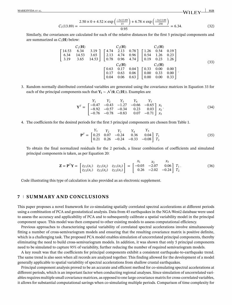
The covariance matrices are constructed for each of the principal components using Equation 29 and the correspond-ing coefficients from Tables 1 and 2. For instance, the covariance between x1 and x2 for principal component 1 is

MARKHVIDA ET AL. 1121

C1(13.89) =2.50 × 0 + 4.52 × exp

(−3×13.89

15

)+ 6.78 × exp

(−3×13.89

250

)0.95

= 6.34. (32)

Similarly, the covariances are calculated for each of the relative distances for the first 5 principal components andare summarized as Ci(H) below:

C1(H)[ 14.53 6.34 3.196.34 14.53 3.653.19 3.65 14.53

] C2(H)[ 4.74 2.13 0.782.13 4.74 0.960.78 0.96 4.74

] C3(H)[ 1.26 0.54 0.190.54 1.26 0.230.19 0.23 1.26

]C4(H)[ 0.63 0.17 0.04

0.17 0.63 0.060.04 0.06 0.63

] C5(H)[ 0.33 0.00 0.000.00 0.33 0.000.00 0.00 0.33

].

(33)

3. Random normally distributed correlated variables are generated using the covariance matrices in Equation 33 foreach of the principal components such that Yi ∼ (0,Ci(H)). Examples are

YT =Y1[−0.47−8.92−0.76

Y2−0.43−0.57−0.78

Y3−1.27−0.34−0.83

Y4−0.66

0.230.07

Y5−0.65

0.03−0.71

] x1x2x3

. (34)

4. The coefficients for the desired periods for the first 5 principal components are chosen from Table 1.

PT =Y1[0.250.21

Y20.070.26

Y3−0.24−0.24

Y40.36

−0.33

Y50.04

−0.08

]T1T2

(35)

To obtain the final normalized residuals for the 2 periods, a linear combination of coefficients and simulatedprincipal components is taken, as per Equation 20:

Z = PTY =[

zT1(x1)zT2(x1)

zT1(x2)zT2(x2)

zT1(x3)zT2(x3)

]=

x1[−0.05

0.26

x2−2.07−2.02

x30.06

−0.24

]T1T2

. (36)

Code illustrating this type of calculation is also provided as an electronic supplement.

7 SUMMARY AND CONCLUSIONS

This paper proposes a novel framework for co-simulating spatially correlated spectral accelerations at different periodsusing a combination of PCA and geostatistical analysis. Data from 45 earthquakes in the NGA-West2 database were usedto assess the accuracy and applicability of PCA and to subsequently calibrate a spatial variability model in the principalcomponent space. This model was then compared to other existing models to assess computational efficiency.

Previous approaches to characterizing spatial variability of correlated spectral accelerations involve simultaneouslyfitting a number of cross-semivariogram models and ensuring that the resulting covariance matrix is positive definite,which is a challenging task. The proposed PCA model enables simulation of uncorrelated principal components, therebyeliminating the need to build cross-semivariogram models. In addition, it was shown that only 5 principal componentsneed to be simulated to capture 95% of variability, further reducing the number of required semivariogram models.

A key result was that the coefficients for principal components exhibit a consistent earthquake-to-earthquake trend.The same trend is also seen when all records are analyzed together. This finding allowed for the development of a modelgenerally applicable to spatial variability of spectral accelerations from shallow crustal earthquakes.

Principal component analysis proved to be an accurate and efficient method for co-simulating spectral accelerations atdifferent periods, which is an important factor when conducting regional analyses. Since simulation of uncorrelated vari-ables requires multiple small covariance matrices, as opposed to one large covariance matrix for cross-correlated variables,it allows for substantial computational savings when co-simulating multiple periods. Comparison of time complexity for

1122 MARKHVIDA ET AL.

the PCA model and alternative methods shows that PCA is a more efficient method for simulating ground motions formultiple periods at multiple locations.

The implementation of the model is invariant to the number of periods that the user is interested in simulating, since theresulting ground motions for any set of periods will be a linear combination of coefficients in Table 1 and a fixed numberof simulated principal components. It is recommended that at least 5 principal components be used in simulation tosufficiently capture the variability. The spatially correlated principal components are simulated using covariance matricesthat can be built using Equation 29, which is only dependent on the separation distance between locations of interest.The computational efficiency gained by using this method makes it desirable for modeling regional correlated groundmotions at multiple periods.

Finally, the proposed model was shown to be accurate by comparing the resultant semivariogram andcross-semivariogram models with the empirical ones. Although the model was built in the principal component basis, itis closely representative of the empirical spatial variability in the original space.

8 ELECTRONIC SUPPLEMENT

The empirical model coefficients presented in Tables 1 and 2 are provided as comma-separated value files in Support-ing Information. In addition, the MATLAB code for implementation of the predictive model for simulating normalizedwithin-event spectral acceleration residuals at multiple sites and periods is available at https://github.com/bakerjw/Spatial_PCA.

ACKNOWLEDGEMENTS

The authors would like to thank Anne Kiremidjian, Jef Caers, Lewis Li, Alexandre Boucher, and Anna Michalak for theirinsightful comments and advice during the course of this research project. This work was supported by the NationalScience Foundation under NSF grant number CMMI 0952402. Any opinions, findings, and conclusions or recommenda-tions expressed in this material are those of the authors and do not necessarily reflect the views of the National ScienceFoundation.

ORCID

Maryia Markhvida http://orcid.org/0000-0001-5398-0960Luis Ceferino http://orcid.org/0000-0003-0322-7510Jack W. Baker http://orcid.org/0000-0003-2744-9599

REFERENCES1. Abrahamson NA, Silva WJ, Kamai R. Summary of the ASK14 ground motion relation for active crustal regions. Earthquake Spectra.

2014;30(3):1025-1055.2. Boore DM, Stewart JP, Seyhan E, Atkinson GM. NGA-West2 equations for predicting PGA, PGV, and 5% damped PSA for shallow crustal

earthquakes. Earthquake Spectra. 2013;30(3):1057-1085.3. Campbell KW, Bozorgnia Y. NGA-West2 ground motion model for the average horizontal components of PGA, PGV, and 5% damped

linear acceleration response spectra. Earthquake Spectra. 2014;30(3):1087-1115.4. Chiou BSJ, Youngs RR. Update of the Chiou and Youngs NGA model for the average horizontal component of peak ground motion and

response spectra. Earthquake Spectra. 2014;30(3):1117-1153.5. Idriss IM. An NGA-West2 empirical model for estimating the horizontal spectral values generated by shallow crustal earthquakes.

Earthquake Spectra. 2014;30(3):1155-1177.6. Baker JW, Cornell CA. Correlation of response spectral values for multicomponent ground motions. Bull Seismol Soc Am.

2006;96(1):215-227.7. Goda K, Hong HP. Spatial correlation of peak ground motions and response spectra. Bull Seismol Soc Am. 2008;98(1):354-365.8. Jayaram N, Baker JW. Correlation model for spatially distributed ground-motion intensities. Earthquake Eng Struct Dyn.

2009;38(15):1687-1708en.9. Esposito S, Iervolino I. PGA and PGV spatial correlation models based on European multievent datasets. Bull Seismol Soc Am.

2011;101(5):2532-2541.10. Wang M, Takada T. Macrospatial correlation model of seismic ground motions. Earthquake Spectra. 2005;21(4):1137-1156.

MARKHVIDA ET AL. 1123

11. Goda K, Atkinson GM. Intraevent spatial correlation of ground-motion parameters using SK-net data. Bull Seismol Soc Am.2010;100(6):3055-3067.

12. Weatherill GA, Silva V, Crowley H, Bazzurro P. Exploring the impact of spatial correlations and uncertainties for portfolio analysis inprobabilistic seismic loss estimation. Bull Earthquake Eng. 2015;13(4):957-981.

13. FEMA. FEMA P-58-1: Seismic performance assessment of buildings. Volume 1-methodology. Federal Emergency ManagementAgency Washington, DC, https://www.fema.gov/media-library-data/1396495019848-0c9252aac91dd1854dc378feb9e69216/FEMAP-58_Volume1_508.pdf; 2012.

14. Yepes C, Silva V, Rossetto T, et al. The global earthquake model physical vulnerability database. Earthquake Spectra. 2016;32(4):2567-2585.15. (FEMA) FEMA. HAZUS MH-2.1 Earthquake Model Technical Manual. Washington, D.C.: FEMA; 2015.16. Loth C, Baker JW. A spatial cross-correlation model of spectral accelerations at multiple periods. Earthquake Eng Struct Dyn.

2013;42(3):397-417.17. Jayaram N, Baker JW. Statistical tests of the joint distribution of spectral acceleration values. Bull Seismol Soc Am. 2008;98(5):2231-2243.18. Ancheta TD, Darragh RB, Stewart JP, et al. NGA-West2 database. Earthquake Spectra. 2014;30(3):989-1005.19. Journel AG, Huijbregts CJ. Mining Geostatistics. San Diego, CA: Academic press; 1978.20. Baker JW, Jayaram N. Effects of spatial correlation of ground motion parameters for multi-site seismic risk assessment: collaborative

research with Stanford University and AIR. Technical Report, Final Technical Report. Report for US Geological Survey National Earth-quake Hazards Reduction Program (NEHRP) External Research Program Award 07HQGR0031; 2008. https://web.stanford.edu/~bakerjw/Publications/Baker_Jayaram_(2008)_spatial_correlation,_USGS_rpt.pdf

21. Isaaks EH, Srivastava R. An Introduction to Applied Geostatistics. New York, NY: 551.72 I86, Oxford University Press; 1989.22. Goovaerts P. Geostatistics for Natural Resources Evaluation. New York: Oxford University Press; 1997.23. Goulard M, Voltz M. Linear coregionalization model: tools for estimation and choice of cross-variogram matrix. Math Geol.

1992;24(3):269-286.24. Journel AG. Markov models for cross-covariances. Math Geol. 1999;31(8):955-964.25. Chiles JP, Delfiner P. Geostatistics: Modeling Spatial Uncertainty, Vol. 497. Hoboken, NJ: John Wiley & Sons; 2009.26. Jackson JE. A User's Guide to Principal Components, Vol. 587. Hoboken, NJ: John Wiley & Sons; 2005.27. Cangelosi R, Goriely A. Component retention in principal component analysis with application to cDNA microarray data. Biol Direct.

2007;2(1):2. https://doi.org/10.1186/1745-6150-2-228. Jolliffe I. Principal Component Analysis. New York, NY: Wiley Online Library; 2002.29. Wackernagel H. Multivariate Geostatistics: An Introduction with Applications. Berlin, Germany: Springer Science & Business Media; 2003.30. Chiou B, Darragh R, Gregor N, Silva W. NGA project strong-motion database. Earthquake Spectra. 2008;24(1):23-44.31. Gentle JE. Random Number Generation and Monte Carlo Methods. New York, NY: Springer Science & Business Media; 2003.32. Trefethen LN, Bau DIII. Numerical Linear Algebra, Vol. 50. Philadelphia, PA: SIAM; 1997.

SUPPORTING INFORMATION

Additional Supporting Information may be found online in the supporting information tab for this article.

How to cite this article: Markhvida M, Ceferino L, Baker JW. Modeling spatially correlated spectral acceler-ations at multiple periods using principal component analysis and geostatistics. Earthquake Engng Struct Dyn.2018;47:1107–1123. https://doi.org/10.1002/eqe.3007