Embed Size (px)
Citation preview

Modeling super-spreading events for SARS
Thembinkosi P. Mkhatshwa
Thesis submitted to the Graduate College of Marshall University inpartial fulfillment of the requirements for the degree of
Master of Artsin
Mathematics
Anna Mummert, Ph.D., ChairBonita Lawrence, Ph.D.
Judith Silver, Ph.D.
Department of Mathematics
Huntington, West Virginia2010
Copyright 2010 by Thembinkosi P. Mkhatshwa
Acknowledgements
I thank the Lord God Almighty for His invaluable assistance while do-ing this research. A million thanks goes to my thesis advisor, Dr AnnaMummert, who supplied me with all the research materials I neededand whose expertise in mathematical biology was of great help. Manythanks to pastor Fadiran and pastor Arisekola for their support andencouragement in the process of doing this research. I would also liketo thank my grandmother, aunt, and my best friend (Londiwe S. Shon-gwe) for their financial and spiritual support. I am also indebted to anumber of people who directly or indirectly made contributions to thiswork.
Everlasting Father, everlasting Son, immortal Holy Ghost
thank you.
iii

Contents
1 Introduction 11.1 What is SARS? . . . . . . . . . . . . . . . . . . . . . . 2
1.1.1 Spread to other countries . . . . . . . . . . . . . 21.1.2 SARS symptoms and signs . . . . . . . . . . . . 31.1.3 Transmission . . . . . . . . . . . . . . . . . . . 3
1.2 The role of mathematical modeling in the spread of theSARS epidemic . . . . . . . . . . . . . . . . . . . . . . 4
1.3 Super-spreading events in infectious diseases . . . . . . 51.4 Aim and Objectives . . . . . . . . . . . . . . . . . . . . 6
2 Basic population models 72.1 The exponential growth model . . . . . . . . . . . . . . 7
2.1.1 Model formulation . . . . . . . . . . . . . . . . 72.1.2 Analytical and equilibrium solutions of the expo-
nential model . . . . . . . . . . . . . . . . . . . 82.1.3 Merits and limitations of the exponential model 9
2.2 The logistic growth model . . . . . . . . . . . . . . . . 112.2.1 Model formulation . . . . . . . . . . . . . . . . 122.2.2 Analytical and equilibrium solutions for the lo-
gistic model . . . . . . . . . . . . . . . . . . . . 132.2.3 Merits and limitations of the logistic model . . . 14
3 The basic reproduction number, R0 163.1 The Next Generation Method . . . . . . . . . . . . . . 16
4 Compartmental models in epidemiology 184.1 The standard SIR epidemic model . . . . . . . . . . . . 18
4.1.1 SIR model assumptions . . . . . . . . . . . . . . 194.1.2 The governing equations . . . . . . . . . . . . . 214.1.3 Initial conditions . . . . . . . . . . . . . . . . . 214.1.4 The SIR model analysis . . . . . . . . . . . . . 224.1.5 Benefits and limitations of the SIR model . . . 27
iv

4.2 The SI1I2R model . . . . . . . . . . . . . . . . . . . . . 294.2.1 The SI1I2R model assumptions . . . . . . . . . 304.2.2 The governing equations . . . . . . . . . . . . . 314.2.3 SI1I2R model analysis . . . . . . . . . . . . . . 31
5 The SIPR epidemic model 385.1 The SIPR model assumptions . . . . . . . . . . . . . . 405.2 Governing equations of the SIPR model . . . . . . . . . 415.3 Initial conditions . . . . . . . . . . . . . . . . . . . . . 425.4 Relationships between the variables . . . . . . . . . . . 435.5 SIPR model analysis . . . . . . . . . . . . . . . . . . . 43
5.5.1 Existence and uniqueness of a global solution . 445.5.2 Positivity and boundedness of solutions . . . . . 445.5.3 SIPR Equilibrium points and their stability anal-
ysis . . . . . . . . . . . . . . . . . . . . . . . . . 455.5.4 R0 for SIPR using The Next Generation method 46
5.6 Benefits and limitations of the SIPR model . . . . . . . 505.7 Possible future directions of work for the SIPR model . 50
v
List of Tables
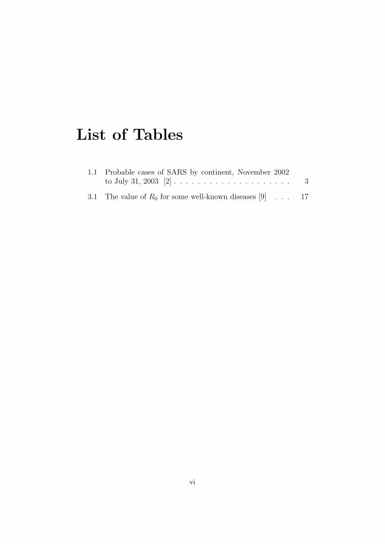
1.1 Probable cases of SARS by continent, November 2002to July 31, 2003 [2] . . . . . . . . . . . . . . . . . . . . 3
3.1 The value of R0 for some well-known diseases [9] . . . 17
vi

List of Figures
2.1 Population grows exponentially, using r = 0.5 and N =100 . . . . . . . . . . . . . . . . . . . . . . . . . . . . . 9
2.2 Population declines to extinction, using r = −0.5 andN = 100 . . . . . . . . . . . . . . . . . . . . . . . . . . 10
2.3 Population size stays constant for all time, using r = 0and N = 100 . . . . . . . . . . . . . . . . . . . . . . . 10
2.4 Population increases and approaches the carrying capac-ity asymptotically, using N0 = 4 and K = 20 . . . . . . 14
2.5 Population decreases and approaches the carrying ca-pacity asymptotically, using N0 = 45 and K = 20 . . . 15
4.1 SIR solutions behavior in continuous time of disease out-break, using β = 0.1 and γ = 0.7 . . . . . . . . . . . . 24
4.2 SIR solutions behavior in continuous time of disease out-break, using β = 0.4 and γ = 0.4 . . . . . . . . . . . . 25
4.3 SIR solutions behavior in continuous time of disease out-break, using β = 0.2 and γ = 0.3 . . . . . . . . . . . . 26
4.4 SI1I2R solutions behavior in continuous time for a genericepidemic disease outbreak, using β = 0.2, r1 = 0.1, r2 =0.3 and γ = 0.3 . . . . . . . . . . . . . . . . . . . . . . 34
4.5 SI1I2R solutions behavior in continuous time for a genericepidemic disease outbreak, using β = 0.3, r1 = 0.275, r2 =0.3 and γ = 0.3 . . . . . . . . . . . . . . . . . . . . . . 35
5.1 SIPR solutions behavior in continuous time of SARSoutbreak, using β = 0.1, b = 0.8, x = 4 and k = 9 . . . 46
5.2 SIPR solutions behavior in continuous time of SARSoutbreak, using β = 0.1, b = 0.8, x = 2 and k = 3 . . . 47
5.3 SIPR solutions behavior in continuous time of SARSoutbreak, using β = 0.3, b = 0.8, x = 4 and k = 9 . . . 48
vii

Modeling super-spreading events for SARS
Thembinkosi P. Mkhatshwa
ABSTRACT
One of the intriguing characteristics of the 2003 severe acute respira-tory syndrome (SARS) epidemics was the occurrence of super spreadingevents (SSEs). Super-spreading events for a specific infectious diseaseoccur when infected individuals infect more than the average number ofsecondary cases. The understanding of these SSEs is critical to under-standing the spread of SARS. In this thesis, we present a modificationof the basic SIR (Susceptible - Infected - Removed) disease model,an SIPR (Susceptible - Regular Infected - Super-spreader - Removed)model, which captures the effect of the SSEs.
viii
Chapter 1
Introduction
The Severe Acute Respiratory Syndrome (SARS) was the first epi-demic of the 21st century. It emerged in China late 2002 and quicklyspread to 32 countries causing more than 774 deaths and 8098 infec-tions worldwide [14]. SARS is an example of the devastating epidemicsof infectious diseases which have wiped out a significant percentage ofthe human population throughout history. The primary goal of thisthesis is to formulate a mathematical model that captures the role ofsuper-spreading events in the spread of the 2002-2003 SARS epidemic.
The first chapter is devoted to giving background and vital informationabout SARS. Our main goal here is to understand the basic epidemiol-ogy of this disease and the role of mathematical modeling in modelingthe spread of the SARS epidemic. A review of two basic populationmodels, the exponential and logistic growth model respectively, is givenin Chapter 2. The next generation method, a method used for calcu-lating an important parameter in the study of epidemics (the basicreproduction number) is presented in Chapter 3. An overview of theSIR (Susceptible - Infected - Removed) and SI1I2R (Susceptible - In-fected Class 1 - Infected Class 2 - Removed) models, standard modelsin the study of infectious diseases, are presented in Chapter 4. Finally,a compartment SIPR (Susceptible - Regular Infected - Super-spreader- Removed) model is presented in Chapter 5. This model capturessuper-spreading events as a main feature that is believed to have beenresponsible for the progression of the SARS epidemic.
We start by looking at an overview of the SARS epidemic as it ap-plies to this thesis.
1

1.1 What is SARS?
Severe Acute Respiratory Syndrome (SARS) is a highly contagiousrespiratory disease which is caused by the SARS Coronavirus. It is aserious form of pneumonia, resulting in acute respiratory distress andsometimes death.
The SARS epidemic originated in China, in late 2002. Although theChinese government tried to control the the outbreak of the SARSepidemic without the awareness of the World Health Organization(WHO), it continued to spread. Failure of the Chinese governmentto seek international aid to fight the spread of SARS contributed tothe epidemic spreading to most parts of the country. A Chinese doctorreported the SARS epidemic crisis to the WHO in early April of 2003,which then resulted in a system being set up to improve reporting andcontrol in the SARS crisis [14]. The SARS outbreak is believed to haveoccurred between November 2002 and June 2003 between November2002 and July 2003 [2].
1.1.1 Spread to other countries
An American businessman traveling in southern China in the fall of2002 was the first known foreigner to contract the disease. He did notshow symptoms or become ill until after he had flown from Guangzhou,China, to Hanoi, Vietnam. It is not known how many people thebusinessman might have infected during his travel from China to Viet-nam [16]. In an age of international travel, global business, and tourism,there is no longer such a thing as a purely localized contagious dis-ease. Diseases originating in the most remote inhabited regions can bespread globally in a matter of hours. The first line of defense is accurateand timely information. While the unfortunate American businessmanwas the carrier who took SARS beyond China’s borders, the “head inthe sand” obstructionist attitude of Beijing officials was the real cul-prit [16].
From Table 1.1, we see that the SARS epidemic claimed over 700 livesand infected over 8000 people worldwide between November 2002 andJuly 2003 [2]. There were 7780 SARS cases in the continent of Asiawhere the first outbreak was reported of which 729 of them died bring-ing the fatality rate in Asia to 9.4%. Other notable continents wherethe SARS epidemic was reported include Europe and Africa.
2

Table 1.1: Probable cases of SARS by continent, November 2002 to July 31,2003 [2]
Continent Cases Deaths Death cases not Fatality(%)related to SARS
Europe 492 45 0 9.1
Asia 7780 729 60 9.4
Africa 1 1 0 100
Total 8273 775 60 9.6
1.1.2 SARS symptoms and signs
People affected by SARS develop a fever greater than 100.4◦F (38.0◦C),followed by respiratory symptoms such as cough, shortness of breath ordifficulty breathing. In some cases, the symptoms become increasinglysevere and patients may require oxygen support and mechanical helpto breath. Symptoms found in more than half of the first 138 patientsincluded (in the order of how they commonly appeared): fever, chillsand shaking, muscle aches, cough, and headache. Less common symp-toms include (also in order): dizziness, productive cough (sputum),sore throat, runny nose, nausea and vomiting, and diarrhea [2].
In most cases, symptoms appear within 2 to 3 days of infection [14].The most prominent symptoms of SARS are high fever and coughingor shortness of breath. According to the World Health Organization(WHO), the vast majority of those infected have an incubation periodless than ten days [14]. There may be many factors related to theperson’s immune system or factors in the environment that affect thesymptoms and severity of SARS [14].
1.1.3 Transmission
SARS is caused by a previously unknown type of coronavirus, the sametype that cause common cold. SARS is spread by droplet contact.When someone with SARS coughs or sneezes, infected droplets are
3

spread into the air. Like other coronaviruses, the SARS virus maylive on hands, tissues, and other surfaces for up to six hours in thesedroplets and up to three hours after droplets have dried. After studyingthe virus, SARS was given a basic reproduction number (R0) of threeby Lipstich, a relatively low number [20]. This value is a measure of thepotential of a disease to spread to susceptible populations when controlmeasures are not taken. We explain the details of R0 in Chapter 3.
SARS can only travel a few meters, which limits its transmissibility [4].In order to become infected, a person usually must have either closecontact with an infected person (such as in a household), intense ex-posure (such as in a small area like an airplane or taxi) or have beenin a high risk area (such as a health care setting).
1.2 The role of mathematical modeling in the spreadof the SARS epidemic
Mathematical models have become important tools in analyzing thespread and control of infectious diseases. The model formulation pro-cess clarifies assumptions, variables, and parameters; moreover, modelsprovide conceptual results such as the basic reproduction number dis-cussed in Chapter 3. Mathematical models and computer simulationsare useful experimental tools for building and testing theories, assess-ing quantitative conjectures, answering specific questions, determiningsensitivity to changes in parameter values, and estimating key param-eters from data [9].
Our study will make use of mathematical models in epidemiology (dis-cussed in detail in Chapter 4) which involve the use of ordinary differen-tial equations. The models describe population behavior in continuoustime, t. Ordinary differential equations describe many physical situa-tions. Their prominence in applied mathematics is due to the fact thatmost of the scientific laws are more readily expressed in terms of ratesof change. The SIPR model we develop eventually is a modification ofthe SIR model discussed in Section 4.1.
We conclude this section by giving a brief survey of SARS modelsdeveloped after the 2002-2003 SARS epidemic:
• Lipsitch developed a model for the spread of Severe Acute Respi-ratory Syndrome (SARS) and used the model to make predictionson the impact of public health efforts to reduce disease transmis-
4

sion [5]. Such efforts included quarantine of exposed individualsto separate them (perhaps by confinement to their homes) fromthe susceptible population, and isolation of those who had SARSin strictly supervised hospital areas with no contacts other thanby healthcare personnel. The Lipsitch model is an extension ofthe SEIR model, which is an extension of the SIR model. Besidesthe populations considered by SIR, the SEIR Model (Susceptible-Exposeds-Infecteds-Removeds) has an intermediate Exposed (E)population of individuals who have the disease but are not yetinfectious. The Lipsitch model modifies SEIR to allow for quar-antine, isolation, and death [11].
• Riley, developed a stochastic metapopulation model with hospi-talized and presymptom stages to study SARS in Hong Kong.The focus of the model was to estimate the basic reproductionnumber, R0, discussed in Chapter 3, in the absence of super-spreading events, control measures and nosocomial transmission.Riley concluded that the number of transmissions fell during thecourse of the outbreak as result of control measures and reducedcontact; movement restrictions can be effective; and hospital trans-mission is significant [17].
• Wang developed a simplified deterministic compartment modelto study the outbreak of SARS in Beijing. Their focus was pa-rameter estimation and assessment of control measures. Theyconcluded that applying control measures early is important, inorder to avoid endemic persistence [19].
• Gumel, developed a deterministic model with quarantine, isola-tion to study the SARS outbreak in Toronto. Their focus was toassess the efficiency of control measures. They concluded that aperfect isolation policy alone is sufficient to control SARS, withor without quarantine; and that resources should be devoted dis-proportionately to isolation programs [7].
1.3 Super-spreading events in infectious diseases
Super-spreading events for a specific infectious disease occur when in-fected individuals infect more than the average number of secondarycases [10]. Super-spreading events pose a serious threat to public healthand their influence on the course of diseases must be studied in or-der effectively control the spread of a disease characterized by SSEs.The 2002-2003 outbreak of severe acute respiratory syndrome (SARS)
5

brought the notion of super-spreading events to the forefront of epi-demiological modeling simply because of the high numbers of secondarycases they caused.
In the following discussion we highlight two models that were developedto model super-spreading events for the SARS epidemic.
• Masuda, et al, developed a contact network model to study theoutbreak of SARS. Their focus was to model super-spreadingevents, spatial effects, and social networks. They concluded thatsocial network structure impacts spread; highly connected SSEsare crucial [13].
• Meyers, et al, also developed a network model specifically tostudy the outbreak of SARS in Vancouver. Their focus was tounderstand heterogeneity in SARS transmission (super-spreadingevents, geographic variation in outbreak occurrences). They con-cluded that network structure, and the location of index caseswithin a network, can influence size of outbreaks and chances ofan epidemic occurring [15].
1.4 Aim and Objectives
The principal aim of this thesis is to construct the appropriate mathe-matical model in the form of a system of ordinary differential equationsthat captures the effect of super-spreading events for SARS. We thenanalyze the stability of the model. The main objectives of this thesisare:
• To develop a model for Severe Acute Respiratory Syndrome (SARS)that captures the effect the super-spreading events (SSEs)
• To analyze the stability of the SARS model which includes findingequilibria, showing that a unique global solution of the modelexists. We also show that solutions for the constituent ODEs ofthe SIPR model stay positive for all time, t ≥ 0.
• To present sample graphs to illustrate the behavior of solutionsin continuous time of the SARS outbreak.
• To describe some benefits and limitations of the model.
6

Chapter 2
Basic population models
In this chapter we present a detailed explanation of two basic theoret-ical population models, the exponential growth model and the logisticgrowth model. Each subsection in this chapter includes an explanationof the model, the assumptions associated with the model, its analyti-cal solution, an illustration of the behavior of the model and finally adiscussion of its merits and shortcomings.
2.1 The exponential growth model
The exponential growth model, also called the Malthusian model, de-scribes exponential growth (including exponential decay) based on aconstant rate of population growth or decay. The model is named afterthe Reverend Thomas Malthus, who authored An Essay on the Prin-ciple of Population [12], one of the earliest and most influential bookson population. We discuss the formulation of this model, its analyticalsolution, equilibrium solution, and finally its merits and limitations inthe following subsections.
2.1.1 Model formulation
In many natural phenomena, quantities grow or decrease at a rate thatis proportional to their size. Human population growth is no exceptionto this phenomena. Precisely, if N = N(t) denotes the human popula-tion size in a particular location at time t, then it seems reasonable to
expect that the population growth rate,dN
dt, is directly proportional to
the population size N, that is,dN
dt∝ N . This implies that
dN
dt= rN,
where r = b − d the difference between the constant birth rate b andthe constant death rate d. The constant r is called the instantaneous
7

rate of increase if b > d [6]. The value of r determines whether a popu-lation increases exponentially (r > 0) as shown in Figure 2.1, remainsconstant in size (r = 0) as shown in Figure 2.3 or declines to extinc-tion (r < 0) as shown in Figure 2.2. The complete exponential growthmodel is given by the following equation:
dN
dt= rN (2.1)
subject to the initial condition condition
N(0) = N0 (2.2)
where N(0) = N0 is the initial population size.
Equation 2.1 is a simple model of population growth. The simplic-ity of this model is due to the fact that r, the instantaneous rate ofincrease, is constant as a result of constant birth and death rates, band d, respectively. Further simplification of the model is brought bythe closure (immigration and emigration not taken into consideration)of the population.
2.1.2 Analytical and equilibrium solutions of the exponentialmodel
We proceed to find the exact solution of the first order linear ordinarydifferential equation, model 2.1 so to express the population size N asa function of time, t. To accomplish the latter, we use the method ofseparation of variables:
dN
dt= rN (2.3)
dN
N= rdt
ln(N) = rt+ c1
N(t) = exp(rt+ c1)
= c2 exp(rt)
To obtain the actual value of the constant c2 we apply the initial con-dition 2.2 in equation 2.3 such that N(0) = N0 which implies thatN(0) = c2 exp(r(0)) = c2 exp(0) so that c2 = N0. Hence the analytical
8

Figure 2.1: Population grows exponentially, using r = 0.5 and N = 100
solution of exponential growth model is given by:
N(t) = N0 exp(rt) (2.4)
The equilibrium solution, N = 0, of this model is obtained by settingdN
dt= 0 in Equation 2.1 and solving for N when r 6= 0. For a popula-
tion experiencing exponential growth/decay, the equilibrium solutionmeans that in the long run population size will decrease to zero.
2.1.3 Merits and limitations of the exponential model
The exponential model has the following benefits:
• Exponential growth (or decay) forms the cornerstone of popu-lation biology [6] in the sense that even though no populationcan increase forever without a limit as shown in Figure 2.1, allpopulations have the potential for exponential increase. This po-tential for exponential increase in population size is one of thekey factors that can be used to distinguish living from non-living
9

Figure 2.2: Population declines to extinction, using r = −0.5 and N = 100
Figure 2.3: Population size stays constant for all time, using r = 0 andN = 100
10

organisms [6]. Exponential growth is observed in small popula-tions with seemingly unlimited resources. Exponential decay isobserved in large populations with limited resources.
• For r 6= 0, the exponential population model predicts either pop-ulation growth without bound or inevitable extinction as shownin Figures 2.1 and 2.2. The difference is based on whether thegrowth rate r is positive or negative.
• The model is very simple with only one parameter, the intrinsicgrowth/decay rate, r.
The exponential model suffers from the following limitations:
• In reality, no population grows/decays indefinitely; i.e. from abiological point of view the missing feature of the exponentialmodel is the idea of carrying capacity. The carrying capacity isthe maximum size of the population that can be supported by theenvironment in terms of resources like availability of food. As thepopulation increases in size the environment’s ability to supportthe population decreases. As the population increases per capitafood availability decreases, waste products may accumulate andbirth rates tend to decline while death rates tend to increase. Itseems reasonable to consider a mathematical model which explic-itly incorporates the idea of carrying capacity.
• In the exponential model, we think of the population being closedi.e. we ignore immigration and emigration.
• Finally, the intrinsic growth/decay rate is constant. In reality theintrinsic growth/decay rate is more likely to be time dependenti.e. it changes over time.
2.2 The logistic growth model
In the following discussion, we discuss in detail the logistic growthmodel developed by a Belgian mathematician Pierre Verhulst (1838),who suggested that the rate of population increase may be limitedby several factors such as availability of food, outbreak of diseases,etc. This model addresses the unbounded population growth behaviorobserved in the exponential model discussed in Section 2.1. We find itsanalytical solution, its equilibrium solution, and finally we discuss itsmerits and limitations.
11
2.2.1 Model formulation
The logistic model is a modification of the exponential populationmodel discussed in Section 2.1. As with the exponential populationmodel, the logistic model includes a rate r. The constant r is calledthe instantaneous rate of increase/decrease [6]. The value of r deter-mines whether a population grows logistically (N < K and r > 0) asshown in Figure 2.4, remains constant in size (r = 0) or declines to car-rying capacity (N > K and r < 0) as shown in Figure 2.5 where K isthe carrying capacity of the environment, a constant.
A second parameter, K, represents the carrying capacity of the sys-tem being studied. Carrying capacity is the population level at whichthe birth and death rates of a species precisely match, resulting in astable population over time. In simple terms, for any particular speciesin a given environment, the carrying capacity is the maximum sustain-able population. That is, the largest population the environment cansupport for extended periods of time.
When the population size is small relative to the carrying capacity, lo-gistic growth is exponential with growth rate close to the rate r. As thepopulation approaches the carrying capacity, the logistic growth rateapproaches zero. Likewise, when the population size is large relative tothe carrying capacity, the population size decreases exponentially andapproaches the carrying capacity. The logistic growth/decay rate atany time depends on the population at that time, the carrying capac-ity, and the rate r.
Letting N = N(t) represent the population size at any time periodt, the logistic model is:
dN
dt= r
(1− N
K
)N (2.5)
subject to the initial condition
N(0) = N0,
where N(0) = N0 is the initial population size.
Equation 2.5 above is a separable ordinary differential equation whichcan be solved analytically using the method of separation of variables.
12
2.2.2 Analytical and equilibrium solutions for the logisticmodel
We proceed to find the exact solution of the first order non-linear or-dinary differential equation 2.5 expressing the population size N as afunction of time, t. To accomplish the latter, we use the method ofseparation of variables and the concept of partial fractions:
1
N
dN
dt= r
(1− N
K
)1
N
dN(1− N
K
) = rdt∫ (1
N+
1K
1− NK
)dN =
∫rdt
ln
(N
1− NK
)= rt+ C1
N =C exp(rt)
1 + CK
exp(rt)
Next we solve for the constant C by applying the initial condition inEquation 2.2:
N(0) = N0 =C
1 + CK
which implies that
C =KN0
K −N0
.
Hence the exact solution of the logistic model is given by:
N(t) =KN0 exp(rt)
K +N0(exp(rt)− 1)(2.6)
The equilibrium solutions N = 0 and N = K, of this model are ob-
tained by settingdN
dt= 0 in Equation 2.5 and solving for N when
r 6= 0. These solutions play a crucial role in predicting the populationgrowth behavior in continuous time.
13

Figure 2.4: Population increases and approaches the carrying capacityasymptotically, using N0 = 4 and K = 20
2.2.3 Merits and limitations of the logistic model
The logistic model has the following benefits:
• Unlike the exponential model, the logistic model takes into con-sideration the limited resources of the environment. This is doneby introducing the carrying capacity K in the exponential modeldiscussed in Section 2.1. Birth/death rates depend on populationsize.
• The general form of the logistic model prevents unbounded growthsince the per capita growth rate drops to zero whenN = K. Thus,the population asymptotically approaches K instead of growingindefinitely as shown in Figure 2.4. If N > K the populationdecreases and approaches the carrying capacity asymptotically asshown in Figure 2.5.
• The logistic model is suitable for both population growth anddecay in environments with limited resources.
• The logistic model is simple with two parameters, K, the carryingcapacity, and r the intrinsic growth/deacy rate.
14

Figure 2.5: Population decreases and approaches the carrying capacityasymptotically, using N0 = 45 and K = 20
The logistic model suffers from the following limitations:
• We observe that the logistic model still exhibits similar problemsas those of the exponential model. Precisely, the logistic modelis also autonomous. Also, in reality environmental conditionsinfluence the carrying capacity. As a consequence it can be time-varying, i.e. K = K(t) > 0, which is not so in the basic logisticmodel discussed in this section.
• Like the exponential model, we think of the population beingclosed; i.e. we ignore immigration and emigration.
• Finally, the intrinsic growth/decay rate is constant. In reality theintrinsic growth/decay rate is more likely to be time dependent,i.e. it changes overtime.
15

Chapter 3
The basic reproductionnumber, R0
An important parameter when modeling diseases is the basic repro-ductive number, denoted as R0. It is defined as the “average numberof secondary infections caused by a single infectious individual duringtheir entire infectious lifetime” in a fully susceptible population [18].It’s a measure of how quickly a disease spreads in its initial phase andcan predict whether a disease will become endemic (prevalent) or willdie out [18].
The basic reproductive number is an important threshold parameterbecause it tells us wether a population is at risk from a given disease ornot [9]. When R0 > 1, the occurrence of the disease will increase andwhen R0 < 1 the disease spreads slower than people recover. WhenR0 = 1, the disease occurrence will be constant. R0 is affected by theinfection and recovery rates. For example, the basic reproduction num-ber for a measles epidemic in Niamey, Niger was found to be between12 and 18 [3]. Table 3.1 shows reproduction numbers for well knowndiseases.
3.1 The Next Generation Method
The next generation method is a general method of deriving R0 in sit-uations in which the population is divided into discrete, disjoint com-partments discussed extensively in Chapter 4 [18].
In the next generation method, R0 is defined as the largest eigenvalueof the next generation matrix. The formulation of this matrix involvesdetermining two classes, infected and non-infected, from the model.
16

Table 3.1: The value of R0 for some well-known diseases [9]Disease R0
AIDS 2 to 5
Smallpox 3 to 5
Measles 16 to 18
Malaria > 100
Assume that there are p compartments of which q are infected. Wedefine the vector x = xi, i = 1, 2, ..., p, where xi denotes the number ofindividuals in the ith compartment. Let Fi(x) be the rate of appear-ance of new infections in compartment i and let Vi(x) = V −i (x)−V +
i (x),where V +
i (x) is the rate of transfer of individuals into compartment iby all other means and V −i (x) is the rate of transfer of individuals outof the ith compartment. The difference Fi(x) − Vi(x) , gives the rateof change of xi. Fi only includes infections that are newly arising, butdoes not include terms which describe the transfer of infectious indi-viduals from one infected compartment to another.
The next generation matrix FV −1 is formed from partial derivatives
of Fi and Vi. V−1 is the inverse of matrix V . We have F =
[∂Fi(x0)
∂xj
]and V =
[∂Vi(x0)
∂xj
]where i, j = 1, 2, ..., q and where x0 is the disease
free equilibrium (when everyone remains susceptible which is to saythat there are no infections at all). The entries of FV −1 give the rateat which infected individuals in xj produce new infections in xi, timesthe average length of time an individual spends in a single visit tocompartment j. R0 is given by the largest eigenvalue of the matrixFV −1 [18] [3].
17

Chapter 4
Compartmental models inepidemiology
In order to model the progress of an epidemic in a large populationcomprising of many different individuals with different characteristics,such a population diversity must be reduced to a few key character-istics which are relevant to the infection under consideration [1]. Forexample, for most common childhood diseases that confer long-lastingimmunity it makes sense to divide the population into those who aresusceptible to the disease, those who are infected and those who haverecovered and are immune. These subdivisions of the population arecalled compartments.
A compartmental model is one for which the individuals in a popu-lation are classified into compartments depending on their status withregard to the infection under study. A person cannot be in more thanone compartment at any given time during the course of the disease.However, a person can move from one compartment to another. Thecompartments are usually classified by a string of letters that providesinformation about the model structure. We consider two such compart-ment models in this chapter namely the SIR and SI1I2R compartmentmodels.
4.1 The standard SIR epidemic model
The SIR model is a classical model used to study diseases includingSARS [14]. In an SIR model, the population is divided into threecompartments namely:
• Susceptible individuals, S(t)
18

• Infected individuals, I(t)
• Removed individuals, R(t)
Schematically, we can think of the model as:
S I Rβ γ
where β is the transmission rate and γ is the recovery rate. We describethe variables S, I, and R in detail as follows:
• S = S(t), denotes the number of susceptible individuals at anygiven time, t. Susceptible people are those who are not infectedbut they can contract the disease if they they come in contact withinfected people. Under normal circumstances, we would expectthe number of susceptible people to decrease in continuous timeduring a disease outbreak.
• I = I(t), denotes the number of infected individuals who also havethe potential to infect others at any time, t. At the initial stagesof the outbreak, we would expect the number of infected people toincrease (if R0 discussed in Chapter 3 is greater than one). Thisis because many people would be susceptible and probably lessinformed about the disease in the early stages of the outbreak.I will also decrease as S gets small.
• R = R(t), denotes the number of individuals leaving the infectedclass I who become permanently immune (typically because ofimmunological response, but “immunity” may also include per-manent quarantine or even death [10].
The only way an individual leaves the susceptible group is by becominginfected. The only way a person leaves the infected group is by beingmoved to a quarantine camp, isolation (home) or death. If a personrecovers from the disease, he does not become susceptible again butrather remains in the removed compartment forever.
4.1.1 SIR model assumptions
The following assumptions are made for the SIR model:
19
• The population size N , is large enough and fixed. It is also closedi.e. there is neither emigration nor immigration taking place.
• The population consists of susceptible, infected, and removed in-dividuals at all times with population size, N, defined by N =N(t) = S(t) + I(t) +R(t).
• We assume that the population is subject to homogeneous mixing,which is to say the individuals (susceptible and infected) of thepopulation under study make contacts at random.
• Contacts between either two susceptible people or two infectedpeople are considered as ‘waste’ since they do not result in a newinfection (even though not all contacts between S and I result ina new infection) and hence do not contribute toward the spreadof the disease.
• A susceptible joins the infected compartment if he acquires aninfection by being in contact with an infected person. In the SIRmodel, the latter statement is represented by the term, SI.
• Infected people are produced by the infection of susceptible peo-ple, S, by infected people, I, with constant transmission rate β.
• An infected person joins the removed compartment through iso-lation, quarantine or death at a constant rate proportional to thesize of the infected population I.
• Infected people who recover on any given day leave the infectedcompartment with constant recovery rate γ and join the removedcompartment. For example, if the average duration of the in-fection period is three days, then on average, one third of the
currently infected population recovers each day, i.e. γ =1
3.
• β and γ are average rates for the population.
• We do not take birth and death rates into consideration.
20
4.1.2 The governing equations
We formulate a system of three ordinary differential equations whichbest describe the SIR model:
dS
dt= −βSI
dI
dt= βSI − γI (4.1)
dR
dt= γI
β denotes the transmission rate, between susceptible people and in-fected people, which is expected to result in a new infection; and γ isthe recovery rate.
Adding the above three equations we have that
S ′(t) + I ′(t) +R′(t) = 0. (4.2)
This, after integration, gives
S(t) + I(t) +R(t) = N ∀t ≥ 0, (4.3)
where N , the integration constant, defines our fixed population sizeassumed earlier in Section 4.1.1.
4.1.3 Initial conditions
At time t = t0, (i.e. at the outbreak of the epidemic) we have a rela-tively small group of infected individuals, I = I0 > 0, in the infectedgroup of the population. They are allowed to move and interact freelywith the individuals in the susceptible group as a result of the popula-tion being subjected to homogenous mixing. Also, at time t = t0, thereare no individuals in the removed group (i.e. R(t0) = 0) and everybodyis susceptible excluding the the small group of infected people, I0. Wetherefore formulate initial conditions for the SIR model as follows:
S(t0) = N − I0 = S0
I(t0) = I0
R(t0) = 0,
21
where S0 > 0 and I0 > 0. When S0 and I0 are added, N is obtained.Therefore our complete SIR model is
dS
dt= −βSI
dI
dt= βSI − γI (4.4)
dR
dt= γI
subject to the following initial conditions
S(t0) = S0, I(t0) = I0, and R(t0) = 0.
4.1.4 The SIR model analysis
In the following subsections, we not only show that a global solution tothe SIR model exist but also that it is unique. We further show thatthe number of people in each compartment is nonnegative and it staysfinite for all time t > 0. We also present solution graphs, calculatethe basic reproduction number, R0, using the next generation methoddiscussed in Section 3.1 and further analyze the equilibrium points ofthe model. Finally we highlight some of the benefits and limitations ofthe SIR model.
Existence and uniqueness of a global solution
The system of equations given in Section 4.1.2, which best describesthe SIR model, can be written in the form:
y′ = f(t, y), y(t0) = y0 where y =
S(t)I(t)R(t)
. The function f(t, y) is
continuous everywhere on R3 and its partial derivatives are continu-ous. The function f(t, y) is bounded (since all solutions are bounded).Hence Peano’s existence theorem in conjunction with Theorem 8.1 (onpage 441) in Philip Hartman’s book [8] guarantees the existence of aunique global solution for the SIR model.
Positivity and boundedness of solutions
The SIR model in Section 4.1 describes a human population, and,therefore, it is very important to prove that all quantities (susceptible,infected and removed) will be positive for all time, t > 0. In other
22

words, we want to prove that all solutions of system (given by Equa-tion 4.4 with nonnegative initial data) will remain positive for all timest > 0.
Theorem 4.1.1. Let the initial data be S(0) = S0 > 0,I(0) = I0 > 0 and R(0) = 0. Then the components of the solu-tion S(t), I(t) and R(t) of Equation 4.4 are positive for all time, t > 0.
Proof. In this proof we try to show that if we start with nonnegativeinitial conditions (as indicated by our initial conditions given in Sec-tion 4.1.3) of the SIR model given by equation 4.4, we also end up withnonnegative solutions.
To see this, we assume that S(t) = 0 for some time t > t0,
I(t) ≥ 0, R(t) ≥ 0 and show thatdS
dt≥ 0. Clearly in view of the SIR
model given by Equation 4.4,dS
dt= −βSI = 0 when S(t) = 0 which
shows that the component of the solution S(t) will be nonnegative forall time t > 0.
To show that the component of the solution I(t) will be nonnegativefor all time, t > 0 we assume that I(t) = 0 for some time t > t0, S(t) ≥0, R(t) ≥ 0 and show that
dI
dt≥ 0. Looking at the system of equations
in the SIR model given by Equation 4.4,dI
dt= βSI − γI = 0 when
I(t) = 0 which shows that the component of the solution I(t) will benonnegative for all time t > 0.
Finally, to show that the component of the solution R(t) stays pos-itive for all time we assume that R(t) = 0 for some time t > t0, S(t) ≥0, I(t) ≥ 0 and show that
dR
dt≥ 0. Looking at the SIR model given
by Equation 4.4,dR
dt= γI ≥ 0 when I(t) ≥ 0 since the constant re-
covery rate γ is positive which shows that the solution R(t) will benonnegative for all time t > 0 which completes the proof.
The boundedness of the components of the solution S(t), I(t) and R(t)follows from the fact that N = S(t)+I(t)+R(t) and that S(t), I(t) andR(t) ≥ 0 for all time t > 0. Therefore we have that each component ofthe solution is at most equal to N . That is S(t), I(t), R(t) ≤ N ∀t ≥ 0.It was shown in Section 4.1.3 that each component of the solution isnonnegative at the outbreak of the disease (t = 0). This shows that
23
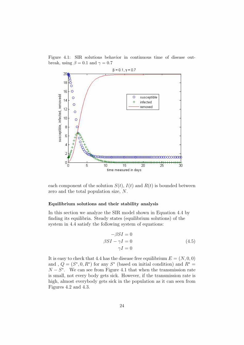
Figure 4.1: SIR solutions behavior in continuous time of disease out-break, using β = 0.1 and γ = 0.7
each component of the solution S(t), I(t) and R(t) is bounded betweenzero and the total population size, N .
Equilibrium solutions and their stability analysis
In this section we analyze the SIR model shown in Equation 4.4 byfinding its equilibria. Steady states (equilibrium solutions) of thesystem in 4.4 satisfy the following system of equations:
−βSI = 0
βSI − γI = 0 (4.5)
γI = 0
It is easy to check that 4.4 has the disease free equilibrium E = (N, 0, 0)and , Q = (S∗, 0, R∗) for any S∗ (based on initial condition) and R∗ =N − S∗. We can see from Figure 4.1 that when the transmission rateis small, not every body gets sick. However, if the transmission rate ishigh, almost everybody gets sick in the population as it can seen fromFigures 4.2 and 4.3.
24

Figure 4.2: SIR solutions behavior in continuous time of disease out-break, using β = 0.4 and γ = 0.4
25

Figure 4.3: SIR solutions behavior in continuous time of disease out-break, using β = 0.2 and γ = 0.3
26
R0 for SIR using The Next Generation method
The SIR model has only one class of the infected population, I. We de-scribe the rate of change of the infected population, I, by the followingequation:
dI
dt= βSI − γI (4.6)
New infections are produced by the infection of susceptible people, S,by infected people, I, with transmission rate, β. We further assumethat infected people recover from the infection with rate γ. For theSIR model shown in Equation 4.6 above, we find that
F = (βS) and V = (γ), where F and V were defined in Section 3.1,and where there is only one infected compartment.
Since the determinant of V is not equal to 0, we can determine theinverse of V , V −1:
V −1 =
(1
γ
),
FV −1 =
(βS
γ
), and
det(FV −1 − λI0) = det
(βS
γ− λ)
=βS
γ− λ.
Setting det(FV −1 − λI0) equal to 0, and solving for λ we obtain oneeigenvalue:
λ =
(βS
γ
). Since λ is the only eigenvalue obtained, it is the largest
eigenvalue of FV −1. We conclude by the next generation method de-
scribed in Section 3.1 that λ =
(βS
γ
)is the basic reproduction number
of the SIR model where S = S0 = N − I0, the population size. That is
R0 =βS
γ.
4.1.5 Benefits and limitations of the SIR model
The SIR model is a good, simple, model for many infectious diseasesincluding measles, SARS, foot and mouth, influenza, H1N1, mumpsand rubella [2]. The SIR model is dynamic in the following way:
27

• The population size, N, is fixed making the model relatively sim-ple to use. A model with fixed population size is good for model-ing short-term outbreaks.
• The SIR model is dynamic in the sense that a majority of thewhole population start susceptible at the outbreak of a disease,some or all them may acquire the infection (move into the in-fectious compartment) and finally die or recover (move into theremoved compartment). Thus each member of the populationtypically progresses from susceptible to infectious and finally tothe removed compartment.
The SIR model suffers from the following limitations:
• We assume that the transmission and recovery rates (β and γ) arefixed. However, in the practical sense these rates are more likelyto vary with time. For example, if there is an outbreak of smallpoxin a particular community there would be more transmission ofthe disease among students at school than there probably wouldwhen school is not in session.
• Many diseases, such as measles or chickenpox, are primarily dis-ease of children. By further subdividing the population intodiffering age-classes researchers have been able to capture age-structured transmission in more detail [9].
• For childhood infections, such as those diseases stated above,there is greater mixing (the contact rate is larger) during schoolterms. Such seasonal dependence leads to regular epidemics ormore complex dynamics, as the disease oscillates between thehigh-contact and low-contact solutions [9].
• For some diseases, other organisms are involved in the transmis-sion, e.g. the mosquito is essential for transmission of malaria,and, together, rats and fleas are responsible for the majority ofbubonic plague cases [9]. For such diseases we need to couple anSIR model for humans with an SIR model for the other organisms.
• Finally, we ignore immigration and emigration which has a greatinfluence in the outbreak of an epidemic, as was the case in theoutbreak of the 2002 - 2003 SARS epidemic and the recent H1N1
flu.
28
4.2 The SI1I2R model
The SI1I2R model was developed by John T. Kemper [10]. This modelincorporates the existence of super-spreaders for a disease without im-munity. In the SI1I2R model, the population is divided into four com-partments namely:
• Susceptible individuals, S(t)
• First class of infected individuals, I1(t)
• Second class of infected individuals, I2(t)
• Removed (immune) individuals, R(t)
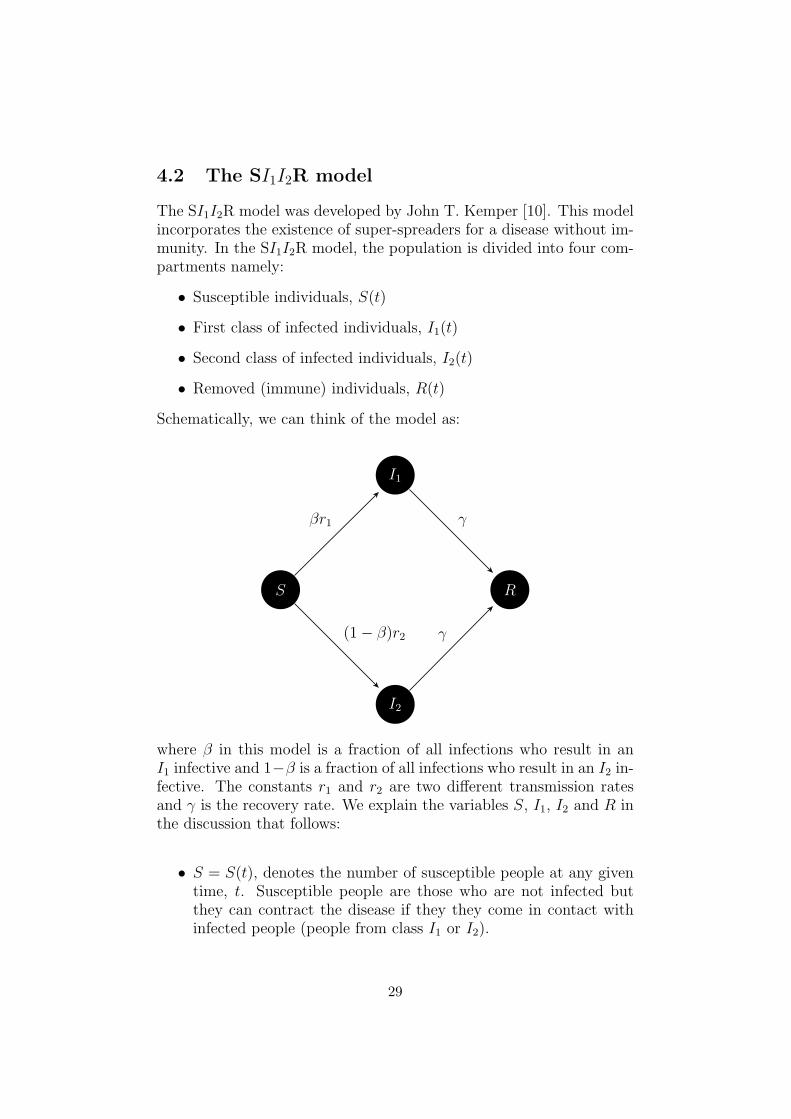
Schematically, we can think of the model as:
S
I1
I2
R
βr1
(1− β)r2
γ
γ
where β in this model is a fraction of all infections who result in anI1 infective and 1−β is a fraction of all infections who result in an I2 in-fective. The constants r1 and r2 are two different transmission ratesand γ is the recovery rate. We explain the variables S, I1, I2 and R inthe discussion that follows:
• S = S(t), denotes the number of susceptible people at any giventime, t. Susceptible people are those who are not infected butthey can contract the disease if they they come in contact withinfected people (people from class I1 or I2).
29

• I = I1(t) and I2(t), denotes two classes of infected people differingonly in their transmission rates, r1 and r2 respectively [10]. Higher(than normal) transmission rates indicate the presence of super-spreading events in the SI1I2R model.
• R = R(t), this is a class of people leaving the infected classes(I1 and I2) become permanently immune (typically because ofimmunological response, but “immunity” may also include per-manent quarantine or even death) [10].
The only way an individual leaves the susceptible group is by becominginfected and hence either join I1 class or I2 class. The only way a personleaves the infected groups is through permanent immunity which alsoincludes permanent quarantine or even death.
4.2.1 The SI1I2R model assumptions
The following assumptions were made for the SI1I2R model:
• The population size N , is large enough and fixed. It is also closedi.e. there is neither emigration nor immigration taking place.
• There are two classes of infected people, I1 and I2, differing onlyin their transmission rates, r1 and r2 respectively.
• We assume that the population is subject to homogeneous mixingwhich is to say the individuals (susceptible and infected) of thepopulation under scrutiny make contacts at random.
• The population consists of susceptible, infected, and recoveredpeople at all times with population size, N, defined N = N(t) =S(t) + I1(t) + I2(t) +R(t).
• Contacts between either two susceptible people or two infectedpeople are considered as ‘waste’ since they do not result in a newinfection and hence do not contribute to the spread of the disease.
• A susceptible joins the infected compartment if he acquires aninfection through being in contact with an infected person fromclass I1 or class I2.
• Also, an infected person joins the removed compartment throughpermanent immunity defined in Section 4.2 [10].
• A fraction, β, of all infections result in an I1 infective, all othersbeing I2 infectives [10].
30

• Infection terminates in permanent immunity (or some other kindof removal) [10].
• γ is the removal rate from I1 and I2 [10].
• We do not take birth and death rates into consideration.
4.2.2 The governing equations
Based on the previous description of Section 4.2.1, the SI1I2R modelwas formulated by the following system of equations:
dS
dt= −(r1I1 + r2I2)S
dI1dt
= β(r1I1 + r2I2)S − γI1 (4.7)
dI2dt
= (1− β)(r1I1 + r2I2)S − γI2dR
dt= γ(I1 + I2)
with initial conditions S(0) = S0 > 0, I1(0) ≥ 0, I2(0) ≥ 0,I1(0)+I2(0) = N−S0 , andR(0) = 0, where β ∈ (0, 1), and γ, r1, and r2 arepositive [10].
The constant β is the fraction of all infections who result in an I1 infec-tive, all others being I2 infectives [10]. There are two classes of infectedpeople, I1 and I2, differing only in their transmission rates, r1 and r2respectively. γ is the removal rate from I1 and I2 to R [10].
4.2.3 SI1I2R model analysis
In the following subsections, we not only show that a global solution ofthe SI1I2R model exist but also that it is unique. We further show thatthe number of people in each compartment is nonnegative and it staysfinite for all time t > 0. We then compute and analyze the equilibriumsolutions for the SI1I2R model. We also present solution graphs andcalculate the basic reproduction number, R0 for the SI1I2R model us-ing the next generation method discussed in Section 3.1. Finally wehighlight some of the benefits and limitations of the SI1I2R model.
Existence and uniqueness of a global solution
The system of equations given in Section 4.2.2 which best describe theSI1I2R model can be written in the form:
31

y′ = f(t, y), y(t0) = y0 where y =
S(t)I1(t)I2(t)R(t)
. The function f(t, y) is
continuous everywhere on R4. The function f(t, y) is continuous every-where on R4 and its partial derivatives are continuous. The functionf(t, y) is bounded (since all solutions are bounded). Hence Peano’sexistence theorem in conjunction with Theorem 8.1 (on page 441) inPhilip Hartman’s book [8] guarantees the existence of a unique globalsolution for the SI1I2R model.
Positivity and boundedness of solutions
The SI1I2R model discussed in Section 4.2 describes a human popu-lation, and, therefore, it is very important to prove that all quantities(susceptible, regularly infected, super-spreading events, and removed)will be positive for all time. In other words, we want to prove that allcomponents of the solution of system 4.2 with nonnegative initial datawill remain positive for all times t > 0.
Theorem 4.2.1. Let the initial data be S(0) = S0 > 0, I1(0) ≥ 0,I2 ≥ 0 and R(0) = 0. Then the components of the solution S(t), I1(t),I2(t), and R(t) of system 4.2.2 are positive for all time, t > 0.
Proof. In this proof we show that if we start with nonnegative initialconditions of the SI1I2R model, given by the equations in Section 4.2.2,we also end up with nonnegative solutions.
To see this, we assume that S(t) = 0 for some time t > t0,
I1(t) ≥ 0, I2(t) ≥ 0, R(t) ≥ 0 and show thatdS
dt≥ 0. Clearly in view
of the system in Section 4.2.2,dS
dt= 0 when S(t) = 0 which shows
that the component of the solution S(t) will be nonnegative for alltime t > 0.
To prove that the component of the solution I1(t) will be nonnegativefor all time t > 0, we assume that I1(t) = 0 for some time t > t0, S(t) ≥0, I2(t) ≥ 0, R(t) ≥ 0 and show that
dI1dt≥ 0. Looking at the SI1I2R
system of equations discussed in Section 4.2.2,dI1dt
= βr2I2S ≥ 0 when
I1(t) = 0 which shows that the solution I1(t) will be nonnegative for
32

all time t > 0.
To prove that the component of the solution I2(t) will be nonnegativefor all time t > 0, we assume I2(t) = 0 for some time t > t0, S(t) ≥0, I1(t) ≥ 0, R(t) ≥ 0 and show that
dI2dt≥ 0. Looking at the SI1I2R
system of equations discussed in Section 4.2.2,dI2dt
= (1− β)r1I1S ≥ 0
when I2(t) = 0 which shows that the solution I2(t) will be nonnegativefor all time t > 0.
Finally, to prove that the component of the solution R(t) will benonnegative for all time t > 0, we assume that R(t) = 0 for some
time t > t0, S(t) ≥ 0, I1(t) ≥ 0, I2 ≥ 0 and show thatdR
dt≥ 0.
Looking at the SI1I2R system of equations discussed in Section 4.2.2,dR
dt= γ(I1 + I2) ≥ 0 when R(t) = 0 which shows that the solution R(t)
will be nonnegative for all time t > 0 which completes the proof.
The boundedness of the components of the solution S(t), I1(t), I2(t)and R(t) follows from the fact that N = S(t) + I1(t) + I2(t) + R(t) andthat S(t), I1(t), I2(t), R(t) ≥ 0 for all time t > 0. Therefore we havethat each component of the solution is at most equal to N . That isS(t), I1(t), I2(t), R(t) ≤ N . It was shown in Section 4.2.1 thateach component of the solution is nonnegative at the outbreak of thedisease (t = t0). This shows that each of the components of the solu-tion S(t), I1(t), I2(t) and R(t) is bounded between zero and the totalpopulation size, N .
Equilibrium solutions and their stability analysis
In this Section we analyze the SIPR model shown in Equation 4.7 byfinding the equilibria. Steady states (equilibrium solutions) of Equa-tion 4.7 satisfy the following system of equations:
−(r1I1 + r2I2)S = 0
β(r1I1 + r2I2)S − γI1 = 0 (4.8)
(1− β)(r1I1 + r2I2)S − γI2 = 0
γI1 + γI2 = 0
It is easy to check that Equation 4.8 above has the disease free equi-librium E = (N, 0, 0, 0) and Q = (S∗, 0, 0, R∗) for any S∗ (based onthe initial condition) and R∗ = N − S∗. We can see from Figure 4.4
33
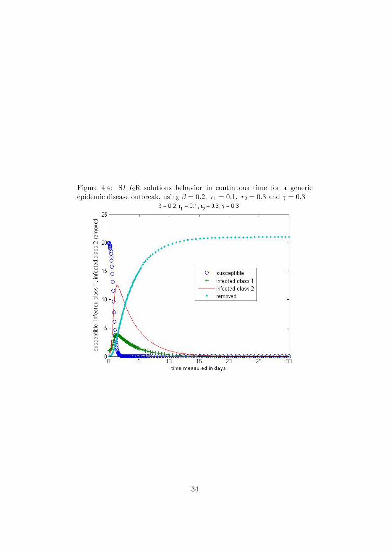
Figure 4.4: SI1I2R solutions behavior in continuous time for a genericepidemic disease outbreak, using β = 0.2, r1 = 0.1, r2 = 0.3 and γ = 0.3
34

Figure 4.5: SI1I2R solutions behavior in continuous time for a genericepidemic disease outbreak, using β = 0.3, r1 = 0.275, r2 = 0.3 and γ = 0.3
35

that when the transmission rates are small, not everybody gets sick.However, if the transmission rate is high, almost everybody gets sickin the population as it can seen from Figure 4.5.
R0 for SI1I2R using The Next Generation method
We describe the rate of change of the first class of infected people, I1,and the second class of infected people, I2, by the following equations:
dI1dt
= β(r1I1 + r2I2)S − γI1 (4.9)
dI2dt
= (1− β)(r1I1 + r2I2)S − γI2
New cases are produced by the infection of susceptible people, S, by aninfected person who is either from the first class of infected individualsor the second class of individuals with contact rates βr1 and (1−β)r2 re-spectively. We further assume that people from both infected classes(I1 or I2) recover from the infection with with the same rate γ. For theSI1I2R model shown in Equation 4.9 above, we find that
F =
(βr1S βr2S
(1− β)r1S (1− β)r2S
)and V =
(γ 00 γ
)Since the determinant of V is not equal to 0, we can determine V −1:
V −1 =
1
γ0
01
γ
,
FV −1 =
βr1S
γ
βr2S
γ(1− β)r1S
γ
(1− β)r2S
γ
, and
det(FV −1 − λI2) = det
βr1S
γ
βr2S
γ(1− β)r1S
γ
(1− β)r2S
γ
.
Setting det(FV −1 − λI2) equal to 0, and solving for λ weobtain two eigenvalues:
λ1 = 0 and λ2 =(1− β)r2S
γ+βr1S
γwhere S = S(0) = S0. Clearly
λ2 is the largest eigenvalue of FV −1 and so we conclude, by the next
36

generation method described in Section 3.1, that λ2 is the basic repro-duction number of the SI1I2R model. We note that
R0 = λ2 =(1− β)r2S
γ+βr1S
γis composed of the
ris
γmultiplied by
their respective probabilities β, (1− β) and then added together.
Benefits and limitations of the SI1I2R model
Like the SIR model, the SI1I2R is a good, simple, model for manyinfectious diseases including SARS, measles, foot and mouth, influenza,H1N1, mumps and rubella [10]. The SI1I2R model is dynamic in thefollowing ways:
• As implied by the variable function of t, the SI1I2R model isdynamic in that the numbers in each compartment may fluctuateover time.
• When an epidemic occurs, the number of susceptible individu-als fall rapidly as more of them get infected and thus enter theinfectious compartments (I1 and I2) and eventually the removedcompartment R.
• The SI1I2R is also dynamic in the sense that a much higher pro-portion of individuals are susceptible at the outbreak of an epi-demic. They may acquire the infection (move into I1 or I2) andfinally die, go to a quarantine camp, or recover (move into theremoved compartment R). Thus each member of the populationtypically progresses from susceptible to infectious (I1 or I2) andfinally to the removed compartment, R.
• The SI1I2R model has two compartments of infectious people(I1 and I2) to facilitate a better understanding of the spread ofany epidemic disease.
Despite all the the benefits of the the SI1I2R, it still suffers from thefollowing limitations.
• We ignore immigration and emigration; which sometimes has agreat influence in the outbreak of an epidemic, as was the case inthe outbreak of the 2009 H1N1 flu.
• The SI1I2R model is an autonomous system. In mathematics, asystem of autonomous differential equations is a system of ordi-nary differential equations which does not depend on the inde-pendent variable.
37

Chapter 5
The SIPR epidemic model
This chapter is devoted to the formulation and analysis of an SIPRmodel that captures one of the several main features which enhancedthe progression and transmission of the SARS epidemic. In particular,this model captures super-spreading events, infected individuals whoin turn had an extra ordinary number of secondary cases. In the SIPRmodel we divide the population size N , into four groups namely:
• Susceptible individuals, S(t)
• Regular infected individuals, I(t)
• Super-spreading events, P (t)
• Removed individuals, R(t)
Schematically, we can think of the model as:
S
I
P
R
bβ
(1− b)β
1x
1k
38
where β is the transmission rate and b the probability that a new infec-tion will be a regular infected person. On the other hand, 1− b is theprobability that a new infection will be a super-spreading event. Theconstant x denotes the average number of days spent by a regularlyinfected person outside isolation. The constant k denotes the averagenumber of days spent by a super-spreading event outside isolation. Weexplain the variables S, I, P , and R in detail in the following piece ofwriting:
• S = S(t), denotes the number of susceptible people at any giventime, t. Susceptible people are those who are not infected butthey can contract the disease if they they come in contact withinfected people (from either I or P ). Under normal circumstances,we would expect the number of susceptible people to decrease incontinuous time during a disease outbreak.
• I = I(t), denotes the number of regularly infected people (infectedpeople who are not super-spreading events) who also have thepotential to infect others at any time, t. At the initial stages ofthe outbreak, we would expect the number of infected people toincrease (if R0 discussed in Chapter 3 is greater than one). Thisis because many people would be susceptible and probably lessinformed about the disease in the early stages of the outbreak. Asthe people get informed and control measures are imposed suchas isolation, quarantine, and medication is available, the numberof infected people is expected to decrease. That is, if the lattercontrol measures are effective enough.
• P = P (t), denotes the number of super-spreading events at anygiven time, t. This is a group of infected people that would nor-mally generate a larger number of secondary cases than a regularlyinfected person would. More super spreaders would mean that thedisease would spread quickly. The class of super-spreading eventsforms a small proportion of the infected class.
• R = R(t), denotes the number of people (regular infected andsuper-spreading events) who have been removed, recovered or diedat any given time, t during a disease outbreak. Precisely, theremoved people are those who are kept in isolation such as inquarantine camps, and maybe at home. Recovered people arethose who receive treatment and hence become immune to thedisease. They are then kept in isolation (asked to stay at home).
39

It is worth mentioning that the class, I = I(t) now has a slightly dif-ferent meaning than the one defined in Sections 4.1 and 4.1.1. Thisis because it no longer refers to the entire class of infected people buta specific class of infected people, called regularly infected people i.e.infected people who are not super-spreading events.
The only way an individual leaves the susceptible group is by becom-ing infected and hence moves either into the regularly infected com-partment or the super-spreading event compartment. The only waya person leaves either the regularly infected class or super-spreadingevents compartment is by being moved to a quarantine camp, isolation(home) or death. If a person recovers from the disease, he does notbecome susceptible again but rather remains in the removed compart-ment forever.
5.1 The SIPR model assumptions
The following assumptions are made for the SIPR model:
• The population size N , is large enough and fixed. It is also closed,i.e. there is neither emigration nor immigration taking place.
• We assume that the population is subject to homogeneous mixingwhich is to say the individuals (susceptible, regularly infected, andthe super-spreading events) of the population under scrutiny willassort and make contacts at random.
• The populations consists of susceptible, regular infected, super-spreaders, and recovered people at all times such that the popu-lation size N = N(t) = S(t) + I(t) + P (t) +R(t). Also, a personcannot be in more than one compartment at the same time.
• Contacts between either two regular infected people, two super-spreading events or between a regular infected person and a superspreader are considered as ‘waste’ since they do not contributetowards the spread of the disease.
• We do not take birth and death rates into consideration in viewof the short duration of the outbreak.
• Super-spreading events spend more time outside quarantine thanregularly infected people.
40

• A susceptible person joins either the regularly infected compart-ment or the super-spreading event compartment if he acquires aninfection through being in contact with a person who is in any ofthe infected compartments (regularly infected or super-spreadingevents).
• Also, an infected person (regular or super-spreader) joins the re-moved compartment through isolation, quarantine or death.
• Each time there is an interaction between the infected compart-ments (I or P ) and the susceptible population S, there is a prob-ability b that the new infection will be regularly infected (I) and aprobability (1−b) that the new infection will be a super spreadingevent (P ).
• Infected people (regularly infected or super-spreading events) areproduced by the infection of susceptible people, S, by either regu-larly infected people, I, or super-spreading events, P , with trans-mission rate β.
• Regularly infected people who recover on any given day leave the
regularly infected compartment with recovery rate1
xand join the
removed compartment. The constant x denotes the average num-ber of days spent by a regularly infected person outside isolation.
• Super-spreading events who recover on any given day leave the
super-spreading events compartment with recovery rate1
kand
join the removed compartment. The constant k denotes the av-erage number of days spent by a super-spreading event outsideisolation.
5.2 Governing equations of the SIPR model
Based on the previous descriptions and assumptions we formulate asystem of four ordinary differential equations which best describe theSIPR model:
41

dS
dt= −β(I + P )S
dI
dt= bβ(I + P )S − 1
xI (5.1)
dP
dt= (1− b)β(I + P )S − 1
kP
dR
dt=
1
xI +
1
kP
where b is the probability of having contacts between super-spreadingevents and regular infected peoples at any given day, x is a constantwith units of time in days which is a measure of the average number ofdays spent by a regularly infected person outside isolation, and k is aconstant with units of time in days which is a measure of the averagenumber of days spent by a person who is a super-spreading event out-side isolation.
Adding these four equations we have that
S ′ + P ′ + I ′ +R′ = 0 (5.2)
This upon integration gives
S + P + I +R = N, (5.3)
where N , the integration constant, is the fixed population size.
5.3 Initial conditions
Assuming that at time, t = t0, of the outbreak of the SARS epidemicthere were no super-spreading events, we formulate the initial condi-tion P (t0) = 0. Also, at the outbreak of the SARS epidemic therewas a relatively small number of regularly infected people, I = I0 > 0.They are allowed to move and interact freely with the individuals inthe susceptible group as a result of the population being subjected tohomogenous mixing.
At the outbreak of the SARS epidemic, there were no people in theremoved compartment, i.e. R(t0) = 0). Thus everybody is suscepti-ble, excluding the the small group of regularly infected people, I0. We
42
therefore formulate initial conditions for the SIPR model as follows:
S(t0) = N − I0 = S0
I(t0) = I0
P (t0) = 0
R(t0) = 0
where S0 > 0 and I0 > 0. When S0 and I0 are added, N is obtained.Therefore our complete SIPR model is
dS
dt= −βSI − βPS
dI
dt= bβSI + bβPS − 1
xI
dP
dt= (1− b)βPS + (1− b)βSI − 1
kP
dR
dt=
1
xI +
1
kP
subject to the following initial conditions
S(t0) = N − I0 = S0, I(t0) = I0, P (t0) = 0, and R(t0) = 0
5.4 Relationships between the variables
• We assume that I > P and k > x ⇒ SI > SP . This meansthat since we have more regularly infected people than super-spreading events at the outbreak of the disease, we expect in thelong run to have more contacts between between the susceptiblepopulation and the regularly infected people than we would withthe susceptible people with the super-spreading events [5].
• We also assume that b > 0.5 ⇒ b > 1 − b which implies thatβSI > (1−b)βSI. This means that each time there is an interac-tion between an infected person (either I or P ) and a susceptibleperson, there is a high likelihood that the resulting infected willbe join the regularly infected population. The “20/80” rule statesthat 20% of cases cause 80% of transmission.
5.5 SIPR model analysis
In the following subsections, we not only show that a global solutionto the SIPR model exists but also that it is unique. We further show
43

that the number of people in each compartment is nonnegative andit stays finite for all time t > 0. We then compute and analyze theequilibrium solutions of the SIPR model. We also present solutiongraphs and calculate the basic reproduction number, R0, using thenext generation method discussed in Section 3.1. Finally we highlightsome of the benefits and limitations of the SIPR model.
5.5.1 Existence and uniqueness of a global solution
The system of equations given in Section 5.1 which best describe theSIPR model can be written in the form:
y′ = f(t, y), y(t0) = y0 where y =
S(t)I(t)P (t)R(t)
. The function f(t, y) is
continuous everywhere on R4 and its partial derivatives are continu-ous. The function f(t, y) is bounded (since all solutions are bounded).Hence Peano’s existence theorem in conjunction with Theorem 8.1 (onpage 441) in Philip Hartman’s book [8] guarantees the existence of aunique global solution for the SIPR model.
5.5.2 Positivity and boundedness of solutions
The SIPR model discussed in Section 5.1 describes a human popula-tion, and, therefore, it is very important to prove that all quantities(susceptible, regularly infected, super-spreading events, and removed)will be positive for all time. In other words, we want to prove that allcomponents of the solution of system 5.1 with nonnegative initial datawill remain positive for all times t > 0.
Theorem 5.5.1. Let the initial data be S(0) = S0 > 0,I(0) = I0 > 0, P (0) = P0 = 0 and R(0) = 0. Then the components ofthe solution S(t), I(t), P (t), and R(t) of the SIPR model are positivefor all time, t > 0.
Proof. In this proof we show that if we start with nonnegative initialconditions (given in Section 5.3) of the SIPR model given by Equa-tion 5.1, we also end up with nonnegative solutions.
To see this, we assume that S(t) = 0 for some time t > t0,
I(t) ≥ 0, P (t) ≥ 0, R(t) ≥ 0 and show thatdS
dt≥ 0. Clearly in view
44
of the SIPR model,dS
dt= 0 when S(t) = 0 which shows that the solu-
tion S(t) will be nonnegative for all time t > 0.
To prove that the component of the solution I(t) will be positive forall time t > 0, we assume that I(t) = 0 for some time t > t0, S(t) ≥0, P (t) ≥ 0, R(t) ≥ 0 and show that
dI
dt≥ 0. Looking at the SIPR
system of equations,dI
dt= bβPS ≥ 0 when I(t) = 0 which shows that
the component of the solution I(t) will be nonnegative for all time t > 0.
To prove that the component of the solution P (t) will be positive for alltime t > 0, we assume P (t) = 0 for some time t > t0, S(t) ≥ 0, I(t) ≥0, R(t) ≥ 0 and show that
dP
dt≥ 0. Looking at the SIPR system of
equations,dP
dt= (1− b)βIS ≥ 0 when P (t) = 0 which shows that the
component of the solution P (t) will be nonnegative for all time t > 0.
Finally, to prove that the component of the solution R(t) will bepositive for all time t > 0, we assume that R(t) = 0 for some time
t > t0, S(t) ≥ 0, I(t) ≥ 0, P (t) ≥ 0 and show thatdR
dt≥ 0. Looking at
the SIPR system of equations,dR
dt=
1
xI +
1
kP ≥ 0 which shows that
the component of the solution R(t) will be nonnegative for all timet > 0 which completes the proof.
The boundedness of the components of the solution S(t), I(t), P(t) andR(t) follows from the fact that N = S(t) + I(t) + P (t) + R(t) andthat S(t), I(t), P (t), R(t) ≥ 0 for all time t > 0. Therefore we havethat each component of the solution is at most equal to N . Thatis S(t), I(t), P (t), R(t) ≤ N . It was shown in Equation 5.1 thateach component of the solution is nonnegative at the outbreak of thedisease (t = t0). This shows that each of the components of the solu-tion S(t), I(t), P (t) and R(t) is bounded between zero and the totalpopulation size, N .
5.5.3 SIPR Equilibrium points and their stability analysis
In this section we analyze the SIPR model shown in Equation 5.1 byfinding the equilibria. Steady states (equilibrium solutions) of Equa-
45

Figure 5.1: SIPR solutions behavior in continuous time of SARS out-break, using β = 0.1, b = 0.8, x = 4 and k = 9
tion 5.1 satisfy the following system of equations:
−βSI − βPS = 0
bβSI + bβPS − 1
xI = 0 (5.4)
(1− b)βPS + (1− b)βSI − 1
kP = 0
1
xI +
1
kP = 0
It is easy to check that Equation 5.4 has the disease free equilibriumE = (N, 0, 0, 0) and Q = (S∗, 0, 0, R∗) for any S∗ (based on the initialcondition) and R∗ = N − S∗. We can see from Figure 5.1 that whenthe transmission rate is small, not every body gets sick. However, if thetransmission rate is high, almost everybody gets sick in the populationas it can seen from Figures 5.2 and 5.3.
5.5.4 R0 for SIPR using The Next Generation method
We describe the rate of change of the regularly infected individuals, I,and the super-spreading events, P , populations by the following
46

Figure 5.2: SIPR solutions behavior in continuous time of SARS out-break, using β = 0.1, b = 0.8, x = 2 and k = 3
47

Figure 5.3: SIPR solutions behavior in continuous time of SARS out-break, using β = 0.3, b = 0.8, x = 4 and k = 9
48

equations:
dI
dt= bβSI + bβPS − 1
xI (5.5)
dP
dt= (1− b)βPS + (1− b)βSI − 1
kP
New cases are produced by the infection of susceptible people, S, byan infected person who is either regularly infected or a super-spreadingevent with contact rates bβ and (1− b)β respectively. We furtherassume that regularly infected people recover from the infection with
rate1
xand super-spreading events recover from the infection with
rate1
k. For the SIPR model shown in Equation 5.5 above, we find
that
F =
(bβS bβS
(1− b)βS (1− b)βS
)and V =
(1x
00 1
k
)Since determinant of V is not equal to 0 we can determine V −1:
V −1 =
(x 00 k
),
FV −1 =
(bxβS bkβS
(1− b)xβS (1− b)kβS
), and
det(FV −1 − λI2) = det
(xbβS − λ kbβSx(1− b)βS k(1− b)βS − λ
).
setting det(FV −1 − λI2) equal to 0, and solving for λ weobtain two eigenvalues:
λ1 = 0 and λ2 =(1− b)βS
1k
+bβS
1x
where S = S(0) = S0. We note
that λ2 is the largest eigenvalue of FV −1 and so we conclude bythe next generation method described in Section 3.1 that λ2 is the basicreproduction number of the SIPR model. We note that
R0 = λ2 =(1− b)βS
1k
+bβS
1x
is the R0 for I and P (as SIR models),
multiplied by their respective probabilities b, (1− b) then addedtogether.
49

5.6 Benefits and limitations of the SIPR model
The SIPR model has the following valuable benefits:
• Like the SIR model, the SIPR is a good, simple, model for manyinfectious diseases including SARS, measles, foot and mouth, in-fluenza, H1N1, mumps and rubella. It is simple in the sense thatit has few parameters and hence easy to study.
• It captures the aspect of SSE behavior (i.e. SSE stays longer outof quarantine).
• The system of equations in the SIPR model is autonomous whichmakes it easier to study the model mathematically.
Despite all the the benefits of the the SIPR, it still suffers from thefollowing limitations.
• It does not capture all aspects of the disease. It assumes thesame transmission rate for both infected compartments and onlycertain combinations of parameters truly show SSE.
• The generalization of the SIR (base) model, i.e. no birth/deathrates, makes the model only reasonable for short term diseases.The rates are assumed to be constant (time independent), popu-lation averages, and permanent immunity is also assumed.
• We ignore immigration and emigration which had a great influ-ence in the outbreak of the SARS epidemic. The 2002-2003 SARSwas spread mainly through air travel.
5.7 Possible future directions of work for the SIPRmodel
One may wish improve the SIPR model by considering the followingaspects:
• Test the SIPR model against real data and make necessary ad-justments if need be. One possible source for the data could bethe Center for Disease Control (CDC) in Georgia.
• Make changes to the model in order to extend the model to otherdiseases.
• Convert the model to non-autonomous system. This includes con-sidering a time transmission and recovery rates that are are timedependent instead of the fixed ones used in our model.
50

• Do a detailed study of the SIPR steady state solutions (equilib-rium solutions) therefore determining whether they are locallystable or not.
• Consider a population that is not closed, one which takes immi-gration as well as emigration into consideration in the modelingof the SARS epidemic.
51

Bibliography
[1] Fred Brauer. Compartmental models in epidemiology. In Math-ematical epidemiology, volume 1945 of Lecture Notes in Math.,pages 19–79. Springer, Berlin, 2008.
[2] Fred Brauer and Jianhong Wu. Modeling SARS, West Nile virus,pandemic influenza and other emerging infectious diseases: aCanadian team’s adventure. In Modeling and dynamics of infec-tious diseases, volume 11 of Ser. Contemp. Appl. Math. CAM,pages 36–63. Higher Ed. Press, Beijing, 2009.
[3] Grais et al. Estimating transmission intensity for a measles epi-demic in Niamey, Niger: lessons for intervention. Royal Socitey ofTropical Medicine and Hygiene, 100:867–873, 2006.
[4] Shirley Chan et al. Development of vaccines to infectious diseases.pages 3–12. Brown University, Providence, Rhode Island, 2004.
[5] Sung et al. Super-spreading events in a hospital setting: who,when, and why. Hong Kong Medical Journal, 15(6):29–33, 2008.
[6] Nicholas J. Gotelli. A Primer of Ecology. Sinauer Associates, Inc,23 Plumtree Road, Sunderland, MA, fourth edition, 2008.
[7] Troy D et al Gumel AB, Ruan S. Modeling strategies for control-ling SARS outbreaks. Proc R Soc Lond B, 271:2223–2232, 2004.
[8] Philip Hartman. Ordinary Differential Equations. Society for In-dustrial and Applied mathematics, 3600, University City ScienceCenter, Philadelphia, PA 19104-2688, second edition, 2002.
[9] Matt J. Keeling and Pejman Rohani. Modeling infectious diseasesin humans and animals. Princeton University Press, Princeton,NJ, 2008.
[10] John T. Kemper. On the identification of superspreaders for in-fectious disease. Math. Biosci., 48(1-2):111–127, 1980.
52
[11] Cooper B et al Lipsitch, Cohen T. Transmission dynamics andcontrol of severe acute respiratory syndrome. Sciencexpress Re-port, 300:1966–1970, 2003.
[12] T. R. Malthus. An Essay on the Principle of Population 2 volumeset. Cambridge University Press, 1990.
[13] Aihaira K Masuda N, Konno N. Transmission of severe acuterespiratory syndrome in dynamical small-world networks. PhysRev E Stat Nonln Soft Matter Phys, 69:1608–1610, 2004.
[14] Nonhle C. Mdziniso. The mathematical modeling of the SARSepidemic. pages 1–10. University of Swaziland, 2009.
[15] Lauren Ancel Meyers, Babak Pourbohloul, M. E. J. Newman,Danuta M. Skowronski, and Robert C. Brunham. Network the-ory and SARS: predicting outbreak diversity. J. Theoret. Biol.,232(1):71–81, 2005.
[16] Charles A. Ray. How SARS spread from China to other coun-tries. 2003. http://www.helium.com/knowledge/234602-how-sars-spread-from-china-to-other-countries.
[17] Donnelly CA et al Riley S, Fraser. Transmission dynamics of theetiological agent of SARS in Hong Kong. Sciencexpress, 300:1961–1966, 2003.
[18] Robert Smith. Modeling Disease Ecology with Mathematics. Amer-ican Institute of Mathematical Sciences, first edition, 2008.
[19] Wendi Wang and Shigui Ruan. Simulating the SARS outbreak inBeijing with limited data. volume 227, pages 369–379. 2004.
[20] James Watmough. The basic reproduction number and the fi-nal size of an epidemic. In Modeling and dynamics of infectiousdiseases, volume 11 of Ser. Contemp. Appl. Math. CAM, pages237–252. Higher Ed. Press, Beijing, 2009.
53


![Effects of City-Size Heterogeneity on Epidemic Spreading ...web.phys.ntnu.no/~ingves/Downloads/MyPapers/... · ity) [2]. SARS spread within weeks from Hong Kong to 37 other countries](https://img.pdfslide.net/doc/110x75/5f4e0d49846cfb02336f292c/effects-of-city-size-heterogeneity-on-epidemic-spreading-webphysntnunoingvesdownloadsmypapers.jpg)