Embed Size (px)
Citation preview

Modeling the Constituentsof the Early Universe
The Harvard community has made thisarticle openly available. Please share howthis access benefits you. Your story matters
Citable link http://nrs.harvard.edu/urn-3:HUL.InstRepos:40046472
Terms of Use This article was downloaded from Harvard University’s DASHrepository, and is made available under the terms and conditionsapplicable to Other Posted Material, as set forth at http://nrs.harvard.edu/urn-3:HUL.InstRepos:dash.current.terms-of-use#LAA
Modeling the Constituents of the Early Universe
A dissertation presented
by
Natalie Mashian
to
The Department of Physics
in partial fulfillment of the requirements
for the degree of
Doctor of Philosophy
in the subject of
Physics
Harvard University
Cambridge, Massachusetts
May 2017
©c 2017 — Natalie Mashian
All rights reserved.
Dissertation Advisor: Professor Abraham Loeb Natalie Mashian
Modeling the Constituents of the Early Universe
Abstract
Understanding how baryons assembled into the first stars and galaxies given the
underlying dark matter distribution in the early Universe remains one of the key
challenges in the field of cosmology. Given the great distances and extreme faintness
of the oldest celestial objects, direct observation of the high redshift Universe remains
difficult. Due to the biased, small number statistics, various other avenues have been
sought out and paved to construct a coherent picture of the large-scale structure of the
Universe at these early times. This thesis explores several of these avenues in a series of
studies aimed at characterizing the first galaxies and the star-forming molecular gas that
drives their evolution in the early Universe.
We model the effects of strong gravitational lensing and find that by magnifying
sources that would otherwise be too faint to detect and lifting them over the instrumental
detection threshold, lensing allows us to probe the luminosity function (LF) below
current survey limits and constrain the low-luminosity cut-off of the Schechter LF. Using
the most recent dust estimates and z ∼ 4-8 LF measurements, we then model the LF
evolution at higher redshifts by employing abundance matching techniques and derive
the redshift evolution of the star formation rate density along with the associated cosmic
reionization history.
To model the molecular interstellar medium (ISM), we employ the large velocity
gradient (LVG) method, a radiative transfer technique used to quantitatively analyze
iii

CO spectral line energy distributions (SLEDs). In particular, we probe the average state
of the molecular gas in HDF 850.1, a z ∼ 5.2 submillimetre source, as well as a series of
local starburst, Seyfert, and ultraluminous infrared galaxies. We identify characteristic
properties of the local and high-redshift ISM, including the kinetic temperature, gas
density, and column density in each case, and derive the gas masses of the various
CO-emitting sources along with the corresponding CO-to-H2 conversion factors.
Furthermore, we develop a theoretical framework to estimate the intensity mapping
signal and power spectrum of any CO rotational line emitted at high redshifts,
particularly during the epoch of reionization. By linking the characteristic properties
of emitting molecular clouds to the global properties of the host halos, we model the
spatially averaged brightness temperature of all the CO transitions and find the predicted
signals to be within reach of existing instruments. We further apply our formalism to
compute the cumulative CO emission from star-forming galaxies throughout cosmic time.
Lastly, we explore the emergence of planetary systems around carbon-enhanced
metal-poor (CEMP) stars, possible relics of the early Universe residing in the halo of
our galaxy. We determine the maximum distance from the host CEMP star at which
carbon-rich planetesimal formation is possible and characterize the potential planetary
transits across these chemically anomalous stars.
We conclude by exploring the possibility of probing the stellar black hole population
using astrometric observations provided by missions such as Gaia. We predict that nearly
3×10⁵ astrometric binaries hosting black holes should be discovered during Gaia’s five
year mission. The invisible companions of astrometrically observed metal-poor, low-mass
stars may be stellar remnants from the dawn of the Universe, offering to shed light on
iv

the formation of the first stellar black holes in the early stages of galaxy assembly.
v
Contents
Abstract iii
Acknowledgments xii
Dedication xiii
1 Introduction 1
1.1 Early Galaxies . . . . . . . . . . . . . . . . . . . . . . . . . . . . . . . . . . 2
1.1.1 Theoretical Perspective . . . . . . . . . . . . . . . . . . . . . . . . . 2
1.1.2 High-Redshift Observations . . . . . . . . . . . . . . . . . . . . . . 5
1.1.3 Stellar Archaeology . . . . . . . . . . . . . . . . . . . . . . . . . . . 7
1.2 Cool Molecular Gas . . . . . . . . . . . . . . . . . . . . . . . . . . . . . . . 9
1.2.1 Tracing the Molecular ISM . . . . . . . . . . . . . . . . . . . . . . . 10
1.2.2 Modeling CO Excitation . . . . . . . . . . . . . . . . . . . . . . . . 12
1.2.3 Observational Studies . . . . . . . . . . . . . . . . . . . . . . . . . . 14
I High Redshift Galaxies 17
2 Constraining the Minimum Luminosity of High Redshift Galaxies through
Gravitational Lensing 18
2.1 Abstract . . . . . . . . . . . . . . . . . . . . . . . . . . . . . . . . . . . . . 19
2.2 Introduction . . . . . . . . . . . . . . . . . . . . . . . . . . . . . . . . . . . 20
vi
CONTENTS
2.3 The Lensing Model . . . . . . . . . . . . . . . . . . . . . . . . . . . . . . . 24
2.4 Results . . . . . . . . . . . . . . . . . . . . . . . . . . . . . . . . . . . . . . 32
2.5 Discussion . . . . . . . . . . . . . . . . . . . . . . . . . . . . . . . . . . . . 43
2.6 Acknowledgements . . . . . . . . . . . . . . . . . . . . . . . . . . . . . . . 44
3 An Empirical Model for the Galaxy Luminosity and Star Formation
Rate Function at High Redshift 45
3.1 Abstract . . . . . . . . . . . . . . . . . . . . . . . . . . . . . . . . . . . . . 45
3.2 Introduction . . . . . . . . . . . . . . . . . . . . . . . . . . . . . . . . . . . 46
3.3 The Formalism . . . . . . . . . . . . . . . . . . . . . . . . . . . . . . . . . 50
3.3.1 The Observed Star-Formation Rate Functions . . . . . . . . . . . . 50
3.3.2 Method to derive the average SFR−Mh relation . . . . . . . . . . 53
3.3.3 Modeling the SFR Functions . . . . . . . . . . . . . . . . . . . . . . 55
3.4 Results . . . . . . . . . . . . . . . . . . . . . . . . . . . . . . . . . . . . . . 56
3.4.1 The Constant SFR−Mh Relation . . . . . . . . . . . . . . . . . . 56
3.4.2 The Modeled SFR Functions at z = 4− 8 . . . . . . . . . . . . . . 59
3.4.3 A Prediction for the UV LF at z = 9− 10 . . . . . . . . . . . . . . 61
3.4.4 Extrapolation to z ∼ 20 and Predictions for JWST . . . . . . . . . 63
3.4.5 Contribution of Galaxies to Cosmic Reionization . . . . . . . . . . . 67
3.5 Summary . . . . . . . . . . . . . . . . . . . . . . . . . . . . . . . . . . . . 71
3.6 Acknowledgements . . . . . . . . . . . . . . . . . . . . . . . . . . . . . . . 73
II The Molecular Interstellar Medium 74
4 The Ratio of CO to Total Gas Mass in High-Redshift Galaxies 75
4.1 Abstract . . . . . . . . . . . . . . . . . . . . . . . . . . . . . . . . . . . . . 75
4.2 Introduction . . . . . . . . . . . . . . . . . . . . . . . . . . . . . . . . . . . 76
4.3 Large Velocity Gradient Model . . . . . . . . . . . . . . . . . . . . . . . . 79
vii
CONTENTS
4.4 Analysis of HDF 850.1 . . . . . . . . . . . . . . . . . . . . . . . . . . . . . 83
4.4.1 Properties of the Galaxy . . . . . . . . . . . . . . . . . . . . . . . . 83
4.4.2 Separate CO, C+ Virialized Regions . . . . . . . . . . . . . . . . . . 86
4.4.3 Separate CO, C+ Unvirialized Regions . . . . . . . . . . . . . . . . 89
4.4.4 Optically thin [CII] . . . . . . . . . . . . . . . . . . . . . . . . . . . 90
4.4.5 Uniformly Mixed CO, C+ Virialized Region . . . . . . . . . . . . . 92
4.4.6 Uniformly Mixed CO, C+ Unvirialized Region . . . . . . . . . . . . 95
4.5 Cosmological Constraints . . . . . . . . . . . . . . . . . . . . . . . . . . . . 95
4.6 Summary . . . . . . . . . . . . . . . . . . . . . . . . . . . . . . . . . . . . 100
4.7 Acknowledgements . . . . . . . . . . . . . . . . . . . . . . . . . . . . . . . 101
5 High-J CO Sleds in Nearby Infrared Bright Galaxies Observed by Her-
schel/PACS 103
5.1 Abstract . . . . . . . . . . . . . . . . . . . . . . . . . . . . . . . . . . . . . 104
5.2 Introduction . . . . . . . . . . . . . . . . . . . . . . . . . . . . . . . . . . . 105
5.3 Target Selection, Observations, and Data Reduction . . . . . . . . . . . . . 107
5.4 Excitation Analysis . . . . . . . . . . . . . . . . . . . . . . . . . . . . . . . 118
5.4.1 CO SLEDs and Line Ratios . . . . . . . . . . . . . . . . . . . . . . 118
5.4.2 LVG Radiative Transfer Model . . . . . . . . . . . . . . . . . . . . 122
5.4.3 Fitting Procedure . . . . . . . . . . . . . . . . . . . . . . . . . . . . 125
5.5 LVG Results & Discussion . . . . . . . . . . . . . . . . . . . . . . . . . . . 127
5.5.1 NGC 253 . . . . . . . . . . . . . . . . . . . . . . . . . . . . . . . . . 135
5.5.2 M 83 . . . . . . . . . . . . . . . . . . . . . . . . . . . . . . . . . . . 140
5.5.3 M 82 . . . . . . . . . . . . . . . . . . . . . . . . . . . . . . . . . . . 141
5.5.4 NGC 4945 & Circinus . . . . . . . . . . . . . . . . . . . . . . . . . . 142
5.5.5 NGC 1068 . . . . . . . . . . . . . . . . . . . . . . . . . . . . . . . . 144
5.5.6 NGC 4418 . . . . . . . . . . . . . . . . . . . . . . . . . . . . . . . . 145
viii
CONTENTS
5.5.7 IC 694 & NGC 3690 . . . . . . . . . . . . . . . . . . . . . . . . . . . 145
5.5.8 Arp 220 . . . . . . . . . . . . . . . . . . . . . . . . . . . . . . . . . 146
5.5.9 NGC 6240 . . . . . . . . . . . . . . . . . . . . . . . . . . . . . . . . 147
5.5.10 Mrk 231 . . . . . . . . . . . . . . . . . . . . . . . . . . . . . . . . . 148
5.6 Summary . . . . . . . . . . . . . . . . . . . . . . . . . . . . . . . . . . . . 149
5.7 Acknowledgements . . . . . . . . . . . . . . . . . . . . . . . . . . . . . . . 152
6 Predicting the Intensity Mapping Signal for multi-J CO lines 154
6.1 Abstract . . . . . . . . . . . . . . . . . . . . . . . . . . . . . . . . . . . . . 154
6.2 Introduction . . . . . . . . . . . . . . . . . . . . . . . . . . . . . . . . . . . 155
6.3 Modeling the CO Emission . . . . . . . . . . . . . . . . . . . . . . . . . . . 159
6.3.1 CO Brightness Temperature . . . . . . . . . . . . . . . . . . . . . . 159
6.3.2 The Star Formation Model . . . . . . . . . . . . . . . . . . . . . . . 162
6.3.3 Theoretical Models for LVG Parameters . . . . . . . . . . . . . . . 164
6.3.3.1 Gas Kinetic Temperature . . . . . . . . . . . . . . . . . . 165
6.3.3.2 Cloud volume density . . . . . . . . . . . . . . . . . . . . 166
6.3.3.3 Velocity Gradient . . . . . . . . . . . . . . . . . . . . . . . 172
6.3.3.4 CO-to-H2 Abundance Ratio . . . . . . . . . . . . . . . . . 172
6.3.3.5 CO Column Density, including photodissociation . . . . . 172
6.3.4 Model CO SLEDs . . . . . . . . . . . . . . . . . . . . . . . . . . . . 176
6.4 Results . . . . . . . . . . . . . . . . . . . . . . . . . . . . . . . . . . . . . . 179
6.4.1 Predicted CO Fluxes and Spatially Averaged CO Brightness Tem-
perature . . . . . . . . . . . . . . . . . . . . . . . . . . . . . . . . . 179
6.4.2 CO Power Spectrum . . . . . . . . . . . . . . . . . . . . . . . . . . 186
6.5 Discussion . . . . . . . . . . . . . . . . . . . . . . . . . . . . . . . . . . . . 190
6.6 Acknowledgements . . . . . . . . . . . . . . . . . . . . . . . . . . . . . . . 195
7 Spectral Distortion of the CMB by the Cumulative CO Emission from
ix
CONTENTS
Galaxies throughout Cosmic History 196
7.1 Abstract . . . . . . . . . . . . . . . . . . . . . . . . . . . . . . . . . . . . . 196
7.2 Introduction . . . . . . . . . . . . . . . . . . . . . . . . . . . . . . . . . . . 197
7.3 The Formalism . . . . . . . . . . . . . . . . . . . . . . . . . . . . . . . . . 201
7.4 Results . . . . . . . . . . . . . . . . . . . . . . . . . . . . . . . . . . . . . . 204
7.5 Discussion . . . . . . . . . . . . . . . . . . . . . . . . . . . . . . . . . . . . 209
7.6 Acknowledgements . . . . . . . . . . . . . . . . . . . . . . . . . . . . . . . 211
III Early Planetary Systems 212
8 CEMP Stars: Possible Hosts to Carbon Planets in the Early Universe 213
8.1 Abstract . . . . . . . . . . . . . . . . . . . . . . . . . . . . . . . . . . . . . 213
8.2 Introduction . . . . . . . . . . . . . . . . . . . . . . . . . . . . . . . . . . . 214
8.3 Star-forming Environment of CEMP Stars . . . . . . . . . . . . . . . . . . 217
8.4 Orbital Radii of Potential Carbon Planets . . . . . . . . . . . . . . . . . . 220
8.5 Mass-Radius Relationship for Carbon Planets . . . . . . . . . . . . . . . . 229
8.6 Transit Properties . . . . . . . . . . . . . . . . . . . . . . . . . . . . . . . . 234
8.7 Discussion . . . . . . . . . . . . . . . . . . . . . . . . . . . . . . . . . . . . 240
8.8 Acknowledgments . . . . . . . . . . . . . . . . . . . . . . . . . . . . . . . . 244
9 EPILOGUE
The Darkest of All Ends: Hunting Black Holes with GAIA 246
9.1 Abstract . . . . . . . . . . . . . . . . . . . . . . . . . . . . . . . . . . . . . 246
9.2 Introduction . . . . . . . . . . . . . . . . . . . . . . . . . . . . . . . . . . . 247
9.3 The Model . . . . . . . . . . . . . . . . . . . . . . . . . . . . . . . . . . . . 249
9.3.1 Black holes with stellar companions . . . . . . . . . . . . . . . . . . 250
9.3.2 Visible binary companions . . . . . . . . . . . . . . . . . . . . . . . 252
9.3.3 Accessible range of periods . . . . . . . . . . . . . . . . . . . . . . . 253
x
CONTENTS
9.3.4 Volume of space probed by Gaia . . . . . . . . . . . . . . . . . . . . 254
9.4 Results & Discussion . . . . . . . . . . . . . . . . . . . . . . . . . . . . . . 256
9.5 Acknowledgements . . . . . . . . . . . . . . . . . . . . . . . . . . . . . . . 260
References 261
xi
Acknowledgments
I am so deeply appreciative of the opportunity to work under the mentorship of my
advisor, Avi Loeb. He took me under his wing from the first meeting we had during my
orientation visiting week and has been guiding me ever since. His big ideas and strong
encouragement have carried me further in the field of cosmology than I ever imagined. I
would also like to thank our collaborator, Amiel Sternberg, who never hesitated to host
me at Tel Aviv University and pushed me to do great science even with rockets raining
down on our heads.
Thank you to my high school physics teacher, Mr. Manny Katz, for introducing me
to all the wondrous phenomena of our Universe and inspiring me to pursue my curiosity
and delve deeper into physics. And a big thank you to Dr. Jacob Barandes whose
door was always open to physics inquiries, philosophical discussions, and unconditional
support.
Last but not least, I am deeply indebted to Carol Davis, who became my “mom
away from home” when I moved to Cambridge nearly six years ago. Her unlimited
supply of chocolate and hugs and supernatural ability to listen empathetically at any
hour of any day made Harvard truly feel like home.
xii

To my parents, Hilda & John,
who raised me with an awe of the cosmos & a thirst for knowledge.
And to my husband, Jonathan,
who, along with adding immeasurable dimensions of love, meaning, & truth to my life,
also helps the cosmos at large with his daily contributions to the molecular gas content of the Universe.
“When I see Your heavens, the work of Your fingers, the moon and stars that You
have established, what is man that You should remember him?....”(Psalms 8:4-5)
xiii

Chapter 1
Introduction
The early Universe, still shrouded in mystery, has captivated the human imagination for
millennia. Questions of “Where do we come from? Where are we going? What are we?”
have evolved to take on the more empirically-driven form of “Did our Universe have a
beginning, or is it infinitely old? Will it come to an end some time in the future? What
is the Universe made of?” Advances in technology over the last several decades have
opened the door to critically exploring the story of genesis through direct observation.
The cosmic microwave background (CMB) offers the first glimpse of the Universe when
it was merely 400,000 years old, marking the beginning of the cosmic dark ages when
neutral hydrogen filled most of the Universe. Deep images from the Hubble Space
Telescope (HST) provide the next snapshot, nearly one billion years later, revealing
a Universe filled with a highly ionized intergalactic medium (IGM) and teeming with
star-forming galaxies, many with stellar masses exceeding 1010 M.
These observations, among others, have led cosmologists to construct a picture
of cosmic history in which the Universe starts out simple, primarily homogeneous
1

CHAPTER 1. INTRODUCTION
and isotropic, with small spatial fluctuations in the energy density and gravitational
potential. These fluctuations then grow over time due to gravitational instability and
eventually lead to the formation of the large-scale structure observed in the present
Universe. While cosmic geometry, the mass-energy content of the Universe, and the
initial density fluctuation spectrum have all been constrained to high accuracy, our
understanding of galaxy formation is still far from complete. Three main epochs have
been identified in the star formation history of the Universe: a steady rise in the cosmic
star formation rate density (SFRD) from z ∼ 10 to 6 (Bouwens et al. 2011a; Coe et al.
2013), followed by the epoch of galaxy assembly from z ∼ 1 to 3 during which the SFRD
peaks and nearly half of the stars in the present Universe form (Shapley 2011; Reddy
et al. 2008), and ending with an order of magnitude decline in the SFRD from z ∼ 1 to
the present (Lilly et al. 1996; Madau et al. 1996).
To explain this observed star formation history and decipher how baryonic matter
assembled into the observed Universe given the underlying dark matter distribution, we
rely on studies that probe two main components of the universe: (i) the products of the
galaxy formation process, i.e. stars, star formation, and ionized gas, and (ii) the fuel
driving the process, mainly the cool molecular gas in galaxies.
1.1 Early Galaxies
1.1.1 Theoretical Perspective
On the theory side, a “galaxy” is defined as a gravitationally-bound system of stars
embedded in a dark matter halo that is capable of sustaining star formation over
2

CHAPTER 1. INTRODUCTION
cosmological time periods. This definition therefore requires the system to have (a)
sufficient mass to be stable against feedback from its own stars and neighboring halos;
(b) a virialized dark matter halo able to accrete baryons; and (c) an efficient mechanism
to cool the baryonic gas, allowing it to condense and fragment to form protostars (Loeb
& Furlanetto 2013).
In the current theoretical framework, the existence of such systems only becomes
possible after the emergence of the first generation of stars at z ∼ 20 - 30 which ends the
cosmic dark ages and initiates the gradual enrichment of the Universe with metals (Stark
2016). These stars, known as Population III stars, form inside “minihalos” cooled by
molecular hydrogen (H2), and proceed to exert extremely strong feedback on their host
halo’s gas, photoevaporating the diffuse gas in the region and blasting out the rest of the
halo’s gas with their explosive deaths via supernovae. The background of Lyman-Werner
photons produced by these first generation stars further photodissociates the H2 and
gradually raises the critical virial temperature for cold gas formation to a value that
effectively chokes off Population III star formation in minihalos. At this point in cosmic
history, star formation is believed to have shifted to halos with virial temperatures Tvir >
104 K where atomic hydrogen can take over as the main cooling agent. With potential
wells deep enough to retain photoheated gas, these systems can maintain reasonable star
formation rates without completely disrupting their gas supplies. This second generation
of halos therefore gives birth to the first galaxies, which are predicted to form at z ∼ 10
- 15, roughly 500 million years after the Big Bang.
Over the next billion years, these early galaxies are expected to have rapidly accreted
gas and built up stellar mass while releasing Lyman continuum radiation that ionized
their intergalactic surroundings. These bubbles of ionized hydrogen grew over time and
3
CHAPTER 1. INTRODUCTION
gradually came to overlap around overdensities in the matter distribution, leading to
the cosmic reionization of hydrogen. High redshift star-forming galaxies have thus long
been considered the primary candidates responsible for the reionization of intergalactic
hydrogen by z ' 6. In order for this to be the case, recent calculations demonstrate
that there must exist an abundant population of faint star-forming galaxies below the
sensitivity limit of current z > 6 surveys. In particular, galaxies with luminosities as
faint as MUV = -10 to -13, corresponding to 4-7 magnitudes below the current HST
detection limits, are necessary to achieve the observed reionization (Robertson et al.
2013; Bouwens et al. 2015a). Furthermore, the high redshift galaxy population must be
fairly efficient ionizing agents, with ionizing photon escape fractions of fesc = 10-20%.
Though significantly higher than the typical value found in luminous z ' 3 galaxies,
such large escape fractions may be possible, especially given the population of runaway
massive stars whose ionizing flux will be much more likely to escape the host galaxy
(Conroy & Kratter 2012). Alternatively, more extreme ionizing radiation fields would
close the “missing photons” gap, supplying the critical ionizing photon production rate
for IGM reionization by z > 6 galaxies.
The large angular-scale patterns in the CMB polarization maps provide further
constraints on the epoch of reionization and the primary source of ionizing photons. Due
to Thomson scattering by free electrons in the reionized IGM, CMB photons are left
polarized with damped temperature fluctuations. Recent measurements of the resulting
Thomson scattering optical depth by the Planck Collaboration et al. (2016c) yield an
integrated CMB optical depth of τ = 0.058±0.012. Current models have found these
measurements to be consistent with a scenario where the bulk of reionization occurs at
6 < z < 9, with early star-forming galaxies dominating the reionization process and
4
CHAPTER 1. INTRODUCTION
leaving an IGM that is nearly 50% neutral by z = 7 (Bouwens et al. 2015a; Robertson
et al. 2015).
1.1.2 High-Redshift Observations
Over the course of the last decade, the cosmic frontier has been pushed back to a redshift
of z ' 10, allowing the first direct tests of the theoretical picture presented above.
These advances are mostly due to the deep imaging campaigns carried out by the Wide
Field Camera 3 (WFC3) onboard HST. With its unprecedented near-infrared sensitivity,
WFC3 has identified thousands of galaxies within the first billion years after the Big
Bang, providing a census of star formation activity and insight into the physical nature
of these early star-forming galaxies in the redshift range 6 < z < 10.
One of the most fundamental and important observables for galaxy studies in the
early Universe is the luminosity function (LF), which provides the volume density of
galaxies as a function of their luminosity. Constraints on the abundance of star-forming
systems in this time interval are provided most thoroughly by the ultraviolet (UV) LF of
UV continuum dropout galaxies, which is generally parametrized by a Schechter function
(Schechter 1976),
dn
dL= φ(L) =
(φ∗
L∗
)(L
L∗
)αe−L/L
∗(1.1)
where φ∗ is the characteristic volume density, L∗ is the characteristic luminosity, and α
is the faint-end slope. This function provides a good fit for populations that demonstrate
an exponential cutoff above the characteristic luminosity L∗, while following a near
power-law slope α at the faint end of the spectrum. When considering high-redshift
sources, the Schechter function is often expressed in terms of the absolute magnitude
5
CHAPTER 1. INTRODUCTION
instead,
φ(M) =ln 10
2.5φ∗(100.4(M∗−M))α+1 exp [−100.4(M∗−M)] (1.2)
where M∗ is the characteristic absolute magnitude and M is typically the absolute
magnitude corresponding to the luminosity at a rest-frame wavelength of 1500 A.
With the expanding dataset of detected high redshift sources, measurements of the
UV LF have gradually improved. The most recent z > 4 LFs are derived from HST
imaging that provide samples of 4,000-6,000 z ' 4 galaxies, 2,000-3,000 z ' 5 galaxies,
700-900 z ' 6 galaxies, 300-500 z ' 7 galaxies, and 100-200 z ' 8 galaxies (Finkelstein
et al. 2015; Bouwens et al. 2015b). These HST samples, which allow the UV LF to be
characterized over a large dynamic range (∆MUV ' 6 at z ' 6), are complemented by
ground-based imaging surveys that constrain the volume density of galaxies as bright as
MUV ' -23 (Bowler et al. 2014, 2015). Current measurements all suggest a rapid decline
in the abundance of UV-luminous galaxies at z > 4, with a volume density at MUV =
-21 that drops by a factor of 15-20 between z ' 4 and z ' 8 (Finkelstein et al. 2015;
Bouwens et al. 2015b). This evolution is less dramatic for galaxies that are ten times less
luminous (MUV = -18.5), in which case, the volume density only decreases by a factor
of 2 to 3 over the same redshift range (Finkelstein et al. 2015; Bouwens et al. 2015b).
These findings suggest that at earlier times, low-luminosity galaxies are the dominant
contributors to the integrated UV luminosity density.
Less agreement presides over measurements of higher redshift UV luminosity
functions. Roughly 20 candidates have thus far been identified at z ' 9 - 11 in deep
WFC3/IR imaging of the Hubble Deep Field (HUDF) and CANDELS fields (Oesch
et al. 2010, 2012a, 2013, 2014, 2016; Ellis et al. 2013; McLure et al. 2013; Bouwens et al.
6
CHAPTER 1. INTRODUCTION
2015b, 2016). To push beyond the current Hubble detection limit, initiatives such as the
Hubble Frontier Fields (HFF) program take advantage of the strong gravitational lensing
power of massive galaxy clusters to magnify distant background galaxies, enhancing the
detectability of high redshift sources that are intrinsically fainter than the observational
threshold. Several such gravitationally lensed systems have already been identified in
the HFF and CLASH surveys, augmenting the sample of high redshift galaxies (Zheng
et al. 2012; Coe et al. 2013; Bouwens et al. 2014a; Zitrin et al. 2014; Ishigaki et al. 2015;
McLeod et al. 2015). Yet, given the small number statistics, quantifying the evolution
of the UV LF at these high redshifts remains difficult. Several studies have found that
the volume density of UV-luminous galaxies accelerates in its decline at z > 8 (Oesch
et al. 2012a, 2013, 2014; Bouwens et al. 2014a, 2015b), consistent with predictions from
some hydrodynamic simulations and semi-analytic models (Finlator et al. 2011b; Dayal
et al. 2013; Tacchella et al. 2013; Sun & Furlanetto 2016). Others report an evolution
over 8 < z < 10 that continues at the same rate suggested by 4 < z < 8 galaxies (Coe
et al. 2013; Ellis et al. 2013; McLeod et al. 2015, 2016). Future parallel observations
with HST’s BoRG campaign and RELICS initiative promise to provide further insight
and better constrain the evolution of these high redshift objects residing in the early
Universe.
1.1.3 Stellar Archaeology
While traditional far-field cosmology tries to shed light on the first billion years after
the Big Bang via high redshift observations, “near-field” cosmology strives to constrain
the early Universe by studying the chemical abundance patterns in the most metal-poor
7
CHAPTER 1. INTRODUCTION
stars in the local Universe. In contrast to their high-mass counterparts who rapidly burn
through their fuel and die as supernovae in a relatively short time frame, low-mass stars,
M . 0.8 M, live for some ∼ 10(M/M)−3 Gyr before ending up as white dwarfs. They
therefore contain detailed information about the history of their host systems and can be
used to study the conditions that existed at the beginning of star and galaxy formation
(Frebel & Norris 2015).
Identifying these early galaxy fossils relies on the assumption that the most
metal-poor stars that exist today are also the oldest stars. Given the lack of elements
heavier than lithium in the Universe before the formation of the first stars, the chemical
abundance profile of a star stands as the main proxy for determining its age (Frebel &
Norris 2015). Moreover, the stellar composition yields valuable information on the star’s
formation era, the extent of chemical enrichment within its natal cloud, and ultimately,
the cosmic chemical evolution following the Big Bang. Extensive efforts have thus been
devoted to searching for “very metal poor” (VMP) stars in the Milky Way and its
satellite dwarf galaxies, stars defined by [Fe/H] ≤ -2.0 where [Fe/H] refers to the star’s
iron abundance relative to that of the Sun (Beers & Christlieb 2005).
Surveys of these VMP candidates have revealed that approximately 20% of stars
that fall into this category exhibit large overabundances of carbon, with [C/Fe] ≥
+0.7. The fraction of sources with such large carbon-to-iron ratios, known as CEMP
(carbon enhanced metal poor) stars, increases to 30% for stars with [Fe/H] < -3.0 and
75% for [Fe/H] < -4.0 (Beers & Christlieb 2005; Norris et al. 2013; Frebel & Norris
2015). This discovery seems particularly odd when compared to the fact that no
more than a few percent of disk stars with near-solar metallicities exhibit such large
carbon overabundances (Norris et al. 1997a). Though no census has been reached in
8
CHAPTER 1. INTRODUCTION
understanding their origin, the dominating hypothesis posits that these CEMP stars
are second-generation, Population II stars, born from an interstellar medium polluted
with the nucleosynthetic products of Population III supernovae. In the case of a ‘faint’
supernova explosion, only the outer layers, rich in lighter elements, are ejected while
the innermost layers, rich in iron, fall back on the remnant and are not recycled in the
ISM (Umeda & Nomoto 2003, 2005). These peculiar metal-deficient objects are thus
promising probes of the formation of the first stars and will be furthered considered in
terms of their potential to host early planetary systems in the last section of this thesis.
1.2 Cool Molecular Gas
Detailed studies of star formation in nearby galaxies suggest that the cool gas content
of the Universe is a critical parameter in galaxy evolution, providing the raw material
from which stars form. In particular, star formation is found to be closely linked to the
molecular gas content, while showing little relation to the atomic neutral gas content in
a given galaxy (Bigiel et al. 2008). This observation is corroborated at high redshifts by
the lack of evolution of the cosmic HI mass density over the same redshift range where
the SFRD grows by more than an order of magnitude (Prochaska & Wolfe 2009). This
suggests that the other phases of the ISM cannot form stars directly unless they cool
sufficiently to form cold and dense molecular gas, leaving the molecular gas phase as the
most relevant to the study of galaxy formation and evolution.
Furthermore, studies show that once molecular gas forms and becomes self-
gravitating, star formation proceeds to first order according to a star formation law via
local processes inherent to the giant molecular cloud (GMC) (Kennicutt 1998b; Bigiel
9

CHAPTER 1. INTRODUCTION
et al. 2008; Leroy et al. 2008; Krumholz et al. 2009; Genzel et al. 2010). Therefore, if
this universal star formation law were to hold out to high redshifts, the cosmic star
formation rate density would just be a reflection of the molecular gas density history of
the Universe.
1.2.1 Tracing the Molecular ISM
Molecular hydrogen, H2, which dominates the molecular gas component of the Universe,
is unfortunately not directly observable in emission. Given the lack of a permanent dipole
moment, the lowest energy transitions of H2 are strongly forbidden, with spontaneous
decay lifetimes of ∼ 100 years (Bolatto et al. 2013). More importantly, the two lowest
para and ortho transitions have upper level energies E/k ≈ 510 K and 1015 K which
are significantly higher than temperatures in GMCs and are thus very difficult to excite.
Consequently, H2 remains practically invisible in the ISM and observers have to instead
rely on tracer molecules to detect and quantify molecular gas in galaxies.
Carbon monoxide, CO, has become the commonly used tracer molecule of the
ISM, serving as the most abundant molecule after H2. With its weak permanent dipole
moment and a ground rotational transition with a low excitation energy E/k ≈ 5.53 K,
CO is easily excited even in cold molecular clouds (Bolatto et al. 2013). Its J = 1 → 0
transition also falls in a relatively transparent atmospheric window, leading astronomers
to employ emission in the CO(1-0) line to measure molecular gas masses. The standard
approach assumes a basic linear relationship between the observed CO luminosity and
the H2 gas mass,
MH2 = αCOL′CO(1−0) (1.3)
10
CHAPTER 1. INTRODUCTION
where MH2 is in units of solar mass and the luminosity L′CO(1−0) is expressed in
K km s−1pc2. αCO is therefore a mass-to-light ratio, commonly referred to as the
“CO-to-H2 conversion factor.” For the GMCs in our Galaxy, this linear relation has
been derived with αCO ∼ 4.6 M (K km s−1pc2)−1 using three independent methods: (a)
correlation of optical/infrared extinction with CO column densities in interstellar dark
clouds (Dickman 1978); (b) correlation of γ-ray flux with the CO line flux for the Galactic
molecular ring (Bloemen et al. 1986; Strong et al. 1988); and (c) the observed relations
between virial mass and CO line luminosity for Galactic GMCs (Solomon et al. 1987).
The characteristic value of αCO is observed to drop to αCO ∼ 0.8 M (K km s−1pc2)−1
in nearby nuclear starburst galaxies and ultraluminous infrared galaxies (ULIRGs)
(Downes & Solomon 1998), implying more CO emission per unit molecular mass. Downes
& Solomon (1998) suggest most of the CO emission in these starburst and ULIRG
systems comes from an overall warm, pervasive molecular inter-cloud medium, in which
case, the line luminosity is determined by the total dynamical mass (gas plus stars).
Others hypothesize that this lower αCO value may reflect different molecular gas heating
processes in these systems, with cosmic rays and turbulence dominating over photons
(Papadopoulos et al. 2012b).
With the recent explosion in the number and type of galaxies detected in molecular
line emission at z > 1, calibrating this conversion factor for the high redshift universe
has become paramount to the study of the star-forming ISM at the earliest epochs. The
standard practice in the field has been to estimate the molecular gas masses of high
redshift sources by applying the local starburst value to CO observations of quasars and
submillimeter galaxies (SMGs), and the Galactic value (αCO ∼ 4.6 M (K km s−1pc2)−1)
to ‘main-sequence’ color-selected galaxies (CSGs) (Tacconi et al. 2008; Daddi et al.
11

CHAPTER 1. INTRODUCTION
2010). There is mounting evidence, however, that there may be a continuum of values
of αCO and that this conversion factor is likely a function of local ISM conditions such
as pressure, gas dynamics, and metallicity (Papadopoulos et al. 2012b). Galaxies that
harbor more compact gas reservoirs and hyper-star forming environments (SFR ∼ 1000
M/yr) are found to have the most extreme gas excitation and correspondingly, the
lowest mass-to-luminosity ratios. Alongside the star formation rate and SFR surface
density, the host galaxy’s metallicity appears to play a central role in determining αCO
as well. There is increasing evidence that in metal-poor environments, the lack of dust
shielding dramatically reduces the CO content while leaving the H2-rich cloud envelopes
intact, resulting in much higher conversion factors (Leroy et al. 2011; Schruba et al.
2012; Sandstrom et al. 2013). Calibrating the conversion factor for these various source
populations at high redshift remains an active field of research.
1.2.2 Modeling CO Excitation
Radiative transfer techniques are often employed to model the spectral line energy
distribution (SLED) of a given molecule and derive the physical conditions within the
emitting molecular cloud. In the large velocity gradient (LVG) method, an iterative
escape probability formalism is used to compute how the various levels of the CO
molecule are populated through collisional excitation with H2 for a given kinetic
temperature Tkin, H2 density, CO abundance [CO]/[H2], and velocity gradient dv/dr
(Sobolev 1960; Castor 1970; Lucy 1971). (The same modeling can be applied to any
molecule.) The velocity gradient introduced in this model is a means of quantifying the
number of emission photons that can eventually leave the cloud, given the optically thick
12

CHAPTER 1. INTRODUCTION
nature of the CO emission (at least in the low-J transitions). The assumption that such
a gradient exists is justified by observations of interstellar molecular line widths which
range from a few up to a few tens of kilometers per second, far in excess of plausible
thermal velocities in the clouds (Goldreich & Kwan 1974). This suggests that the
observed velocity differences in the molecular medium arise from large-scale turbulence
which enables CO photons to leave their parental clouds.
Once the population fractions in each level are calculated, the optical depths for
each transition as well as the resulting line intensities can be computed. Therefore,
given a measurement of the line emission ladder for a given molecule, constraints may
be placed on the temperature and density of the gas and mass estimates can be derived
from the column density.
In the case where the cloud is exposed to a radiation field, PDR (photon-dominated
region) and XDR (X-ray dominated region) models are employed to determine the gas
conditions. These models take into account elaborate chemical networks and the cooling,
heating, and chemical processes that are entirely dictated by the radiation field to
derive the temperature and density distribution of the H2 molecules (Wolfire et al. 2010;
Meijerink & Spaans 2005; Meijerink et al. 2007). Once these quantities are determined, a
code similar to LVG is then used to compute the rotational line intensities emitted by the
given molecule. However, since most PDR/XDR models are based on one-dimensional
infinite slabs, gas mass estimates can not be derived for these unconfined volumes.
13
CHAPTER 1. INTRODUCTION
1.2.3 Observational Studies
With the explosion in the number and type of galaxies detected in molecular emission at
z > 1, the last few years have seen unprecedented progress in the study of cool molecular
gas in the early Universe. The physical conditions of the gas in some of the brightest high
redshift systems have been investigated using the detailed multi-transition, multi-species
observations provided by centimeter and (sub)millimeter telescopes. Emerging from
these high-redshift CO excitation analyses is the general result that different source
populations at high z show distinctly different excitation patterns (Carilli & Walter
2013).
Of all objects detected at high redshifts, quasars show the most extreme molecular
gas excitation (Weiss et al. 2007; Riechers et al. 2009). Their CO emission ladders can be
modeled with simple models characterized by one gas component, i.e. one temperature
and density, out to the highest J transitions, with typical temperatures of Tkin ∼ 40
- 60 K and gas densities of log (nH2 [cm−3]) = 3.6 - 4.3 (Riechers et al. 2006, 2011b).
This finding suggests that the molecular gas emission in quasars originates from a very
compact gas reservoir in the center of the system, an interpretation which has been
confirmed in the few cases where the CO emission could be resolved (Walter et al. 2004;
Riechers et al. 2008a,b, 2011b). The resulting star formation rate densities are thus
typically high (∼ 103 M yr−1kpc−2) and the molecular gas masses are on the order of ∼
1010(αCO/0.8) M with short gas consumption times ∼ 107 yr (Walter et al. 2009).
Surveys at submm wavelengths have identified another population of galaxies known
as submillimeter galaxies (SMGs). These extreme starburst galaxies (SFR > 103 M/yr)
are also found to have compact, but large, molecular gas reservoirs, suggesting they may
14
CHAPTER 1. INTRODUCTION
be the result of mergers in which the gas settled into the center of the two colliding
galaxies and led to a starburst (Tacconi et al. 2006, 2008). Relative to quasars, the
average excitation of the molecular gas in SMGs is not as extreme, a fact that may be
attributed to the fact that star formation in some SMGs occurs on more extended scales
than quasars (Weiss et al. 2007). The typical temperatures and gas densities in SMGs is
Tkin ∼ 30 - 50 K and log (nH2 [cm−3]) = 2.7- 3.5, respectively. Furthermore, observations
of CO emission reveal an excess in the CO(1-0) line and a more spatially extended
emission in the ground transition than the higher energy transitions (Ivison et al. 2011;
Riechers et al. 2011a). These findings indicate that a two-component gas model is
necessary to account for the observed excitation and that neglecting this additional
component would lead to an underestimation of the total gas mass.
More recently, progress has been made in excitation measurements for more normal
star-forming galaxies at high redshift. These galaxies, selected via their optical or
near-infrared colors, are referred to as “color-selected star-forming galaxies”, CSGs,
and have a volume density more than an order of magnitude larger than SMGs. CSGs
contain molecular gas reservoirs that are more extended, ∼ 10 kpc in size, but similar in
mass to their SMG counterparts (Daddi et al. 2010; Tacconi et al. 2010, 2013). However,
studies have found that gas fractions are very high in these galaxies, comparable to or
larger than the corresponding stellar mass, with 50-65% of the baryons in the galaxies’
half-light radius in the form of gas. With intrinsic star formation rates of ∼ 100 Myr,
CSGs are forming stars at ∼ 10 times lower rates than quasars and SMGs (Daddi et al.
2008). The combination of these factors leads to the less extreme gas excitation observed
in these high-redshift objects, though measurements only exist up to the J = 3→ 2 line
(Dannerbauer et al. 2009). Follow-up observations of higher-order CO transitions will be
15
CHAPTER 1. INTRODUCTION
necessary to further characterize these CSGs.
16
Part I
High Redshift Galaxies
17
Chapter 2
Constraining the Minimum
Luminosity of High Redshift
Galaxies through Gravitational
Lensing
This thesis chapter originally appeared in the literature as
N. Mashian and A. Loeb, Constraining the minimum
luminosity of high redshift galaxies through gravitational
lensing, Journal of Cosmology and Astroparticle Physics, 12,
017, 2013
18

CHAPTER 2. CONSTRAINING MINIMUM LUMINOSITY THROUGH LENSING
2.1 Abstract
We simulate the effects of gravitational lensing on the source count of high redshift
galaxies as projected to be observed by the Hubble Frontier Fields program and the James
Webb Space Telescope (JWST) in the near future. Taking the mass density profile of the
lensing object to be the singular isothermal sphere (SIS) or the Navarro-Frenk-White
(NFW) profile, we model a lens residing at a redshift of zL = 0.5 and explore the radial
dependence of the resulting magnification bias and its variability with the velocity
dispersion of the lens, the photometric sensitivity of the instrument, the redshift of the
background source population, and the intrinsic maximum absolute magnitude (Mmax)
of the sources. We find that gravitational lensing enhances the number of galaxies with
redshifts z & 13 detected in the angular region θE/2 ≤ θ ≤ 2θE (where θE is the Einstein
angle) by a factor of ∼ 3 and 1.5 in the HUDF (df/dν0 ∼ 9 nJy) and medium-deep JWST
surveys (df/dν0 ∼ 6 nJy). Furthermore, we find that even in cases where a negative
magnification bias reduces the observed number count of background sources, the lensing
effect improves the sensitivity of the count to the intrinsic faint-magnitude cut-off
of the Schechter luminosity function. In a field centered on a strong lensing cluster,
observations of z & 6 and z & 13 galaxies with JWST can be used to infer this cut-off
magnitude for values as faint as Mmax ∼ -14.4 and -16.1 mag (Lmin ≈ 2.5×1026 and
1.2×1027 erg s−1 Hz−1) respectively, within the range bracketed by existing theoretical
models. Gravitational lensing may therefore offer an effective way of constraining the
low-luminosity cut-off of high-redshift galaxies.
19
CHAPTER 2. CONSTRAINING MINIMUM LUMINOSITY THROUGH LENSING
2.2 Introduction
The characterization of the earliest galaxies in the universe remains one of the most
important frontiers of observational cosmology, and also one of the most challenging
(Loeb & Furlanetto 2013). High-redshift searches carried out with the Hubble Space
Telescope (HST) have recently provided significant insights to the mass assembly and
buildup of the earliest galaxies (z & 6) and the contribution of star formation to cosmic
reionization (Bunker et al. 2004; Yan & Windhorst 2004b; Bouwens et al. 2010; Ellis et al.
2013). However, because of their great distances and extreme faintness, as well as the
high sky background, high redshift galaxies remain difficult to detect. Furthermore, those
sources which are bright enough to be studied individually are drawn from the bright tail
of the luminosity function (LF) of high redshift galaxies and are therefore not necessarily
representative of the bulk of the population (Bayliss et al. 2010). Gravitational lensing
by galaxy clusters has been highlighted as an efficient way of improving this situation,
providing an opportunity to observe the high-redshift universe in unprecedented detail
(Bradley et al. 2008; Zheng et al. 2012).
Light rays propagating through the inhomogeneous gravitational field of the Universe
are often deflected by intervening clumps of matter, which cause most sources to appear
slightly displaced and distorted in comparison with the way they would otherwise appear
in a perfectly homogeneous and isotropic universe (Schneider & Falco 1992; Bartelmann
& Schneider 2001; Treu 2010). When the light from a distant galaxy is deflected by
foreground mass concentrations such as galaxies, groups, and galaxy clusters, its angular
size and brightness are increased and multiple images of the same source may form. This
phenomenon, referred to as strong gravitational lensing, leads to a magnification bias that
20

CHAPTER 2. CONSTRAINING MINIMUM LUMINOSITY THROUGH LENSING
can have a significant effect on the observability of a population of galaxies. Magnified
sources, that would otherwise be too faint for detection without a huge investment of
observing time, can be found, and unresolved substructure and morphological details in
these intrinsically faint galaxies can be studied (Smail et al. 1997; Pettini et al. 2000;
Ellis et al. 2001). The light magnification produced by nature’s ”cosmic telescopes”
can be exploited in the study of high-redshift galaxies which have greater probability of
falling in alignment with, and therefore being lensed by, a foreground galaxy (Barkana &
Loeb 2000). Zackrisson et al. (2012) explored the prospect of detecting a hypothetical
population of population III galaxies via gravitational lensing by a particular galaxy
cluster (MACS J0717.5 + 3745) as the lens. Indeed, several highly magnified galaxy
candidates at up to redshift z ∼ 10 have already been discovered behind massive clusters
Bayliss et al. (2010); Bradley et al. (2008); Zheng et al. (2012); Richard et al. (2006);
Stark et al. (2007); Richard et al. (2008); Bouwens et al. (2009b); Coe et al. (2013).
The Hubble Frontier Fields program1 is expected to lead to many more such discoveries.
With its six deep fields centered on strong lensing galaxy clusters in parallel with six deep
“blank fields”, the Hubble Frontier Fields will reveal previously inaccessible populations
of z = 5-10 galaxies that are 10-50 times intrinsically fainter than any presently known.
In the coming decade, the planned James Webb Space Telescope (JWST)2 promises to
go even further by placing new constraints on the stellar initial mass function at high
redshift, on the luminosity function of the first galaxies, and on the progress of the
early stages of reionization with observations of galaxies at z & 10 (Gardner et al. 2006;
Windhorst et al. 2006; Haiman et al. 2008).
1http://www.stsci.edu/hst/campaigns/frontier-fields/
2http://www.stsci.edu/jwst/
21
CHAPTER 2. CONSTRAINING MINIMUM LUMINOSITY THROUGH LENSING
While lenses magnify the observed flux and lift sources which are intrinsically too
faint to be observed over the detection threshold, they simultaneously increase the solid
angle within which sources are observed and thus reduce their number density and
measured surface brightness in the sky (Refregier & Loeb 1997). Zemcov et al. (2013)
recently reported measuring a deficit of surface brightness within the central region
of several massive galaxy clusters with the SPIRE instrument, and used the deficit to
constrain the surface brightness of the cosmic infrared background. The outcome of this
trade-off between depth and area depends on a variety of factors, such as the photometric
sensitivity of the detecting device and the slope of the luminosity function of background
sources. Given a photometric sensitivity capable of detecting faint sources even in the
absence of any light amplification, the lensing effect leads to a negative magnification
bias, reducing the apparent surface density behind lensing clusters. If, however, the
fainter sources cannot be observed unless magnified, then whether the magnification
bias leads to a surplus or deficit of observed sources depends on the effective slope of
their luminosity function(Turner et al. 1984). At fainter magnitudes where the effective
slope, α, is shallow, there may not be enough faint sources in the lensed population to
compensate for the increase in total surface area. However, in cases where α & 2, the
gain in depth due to apparent brightening may outweigh the loss in area; gravitational
lensing will thus increase the apparent surface density behind the lensing object, boosting
up the number of detected sources relative to that which would otherwise be observed in
an unlensed field (Bouwens et al. 2009b; Broadhurst et al. 1995).
The observed number counts of galaxies residing at redshifts greater than some z′
may also be sensitive to the intrinsic faint-magnitude cut-off chosen for the extrapolation
of the galaxy LF. Theoretical and numerical investigations have established that a halo
22
CHAPTER 2. CONSTRAINING MINIMUM LUMINOSITY THROUGH LENSING
at z . 10 irradiated by a UV field comparable to the one required for reionization needs
a mass Mh & (0.6 - 1.7) × 108 M, with a corresponding temperature Tvir & (1 - 2)×104
K at z = 7, in order to cool and form stars (Haiman et al. 1996; Tegmark et al. 1997;
Munoz & Loeb 2011). Such claims have motivated models with cut-offs for the absolute
magnitude of the smallest halo capable of forming stars as faint as MAB ≈ -10 Wyithe
& Loeb (2006); Trenti et al. (2010) . Gravitational lensing may provide an effective way
to constrain the value of this minimum luminosity given the fact that the lensed number
count of high-redshift galaxies remains sensitive to this intrinsic low-luminosity cut-off
at much fainter values compared to the observed number count in a blank field.
In this paper, we predict the lensing rate of high-redshift objects that will be
observed with both HST Frontier Fields in the upcoming months, and JWST within the
next decade. In section 2.3 we consider two different axially symmetric lens models: a
singular isothermal sphere and a NFW profile (Navarro et al. 1997) lens for comparison,
examining their respective effects on the number count of the background lensed galaxy
population. In addition to considering lensing clusters, we also consider galaxy-group
lensing and compute the lensing rates expected in each case given the velocity dispersion
of the lensing object. We present our numerical results in section 2.4 and show the
transition from a positive to a negative magnification bias as a function of the minimum
intrinsic luminosity, the photometric sensitivity, and the angular distance from the given
lens. We conclude in section 2.5 with a discussion of our findings and their implications
for observations with the HST Frontier Fields and JWST in the near future.Throughout
this paper, we adopt Ωm = 0.3 and ΩΛ = 0.7 as the present-day density parameters
of matter and vacuum, respectively and take H0 = 100h km s−1 Mpc−1 as the Hubble
constant with h = 0.7. We express all magnitudes in the AB system.
23
CHAPTER 2. CONSTRAINING MINIMUM LUMINOSITY THROUGH LENSING
2.3 The Lensing Model
The ray-tracing equation that relates the position of a source, ~η, to the impact parameter
of a light ray in the lens plane, ~ξ, is given in angular coordinates by
~β = ~θ − ~α(~θ) (2.1)
where ~β = ~η/Ds, ~θ = ~ξ/Dl, and ~α is the reduced deflection angle due to a lens with
surface mass density Σ,
~α(~θ) =4G
c2
DlsDl
Ds
∫(~θ − ~θ′)Σ(~θ′)
|~θ − ~θ′|2d2θ′ . (2.2)
Dl,s,ls are the angular-diameter distances between observer and lens, observer and
source, and lens and source, respectively. In the standard ΛCDM cosmology, the
angular-diameter distance DA(z) of a source at redshift z is defined as
DA(z) =c
H0
1
(1 + z)
∫ z
0
dz′
E(z′)(2.3)
where
E(z) =√
Ωm(1 + z)3 + ΩΛ . (2.4)
For a circularly-symmetric mass distribution, Σ(~θ) = Σ(|~θ|); the dimensionless
surface mass density, also referred to as the convergence, is then given by
κ(x) =Σ(x)
Σcr
with Σcr =c2Ds
4πGDlDls
(2.5)
where we have introduced the dimensionless impact parameter ~x = ~θ/θ0 with an arbitrary
angular scale θ0. The corresponding dimensionless mass m(x) within a circle of angular
radius x is then
m(x) = 2
∫ x
0
dx′x′κ(x′) (2.6)
24
CHAPTER 2. CONSTRAINING MINIMUM LUMINOSITY THROUGH LENSING
and the magnification factor in terms of these dimensionless quantities takes the following
form,
µ(x) =1
(1− m(x)x2
)(1 + m(x)x2− 2κ(x))
. (2.7)
A simple model for the matter distribution in a gravitational lens is a Singular
Isothermal Sphere (SIS) (Schneider & Falco 1992) with a surface mass density of
ΣSIS(ξ) =σ2v
2Gξ. (2.8)
where σv is the line-of-sight velocity dispersion of the lens. In this case, the reduced
deflection angle, commonly referred to as the Einstein angle for the SIS lens and denoted
as θE, is independent of the impact parameter,
θE = 4πσ2v
c2
Dls
Ds
(2.9)
and the lens equation reduces to
~β = ~θ − ~α(~θ) = ~θ −~θ
|~θ|θE (2.10)
where negative angles refer to positions on the opposite side of the lens center. The
lensing effect causes the image of the source to be displaced, magnified, and sometimes
split (Refregier & Loeb 1997). When |β| < θE, the lens equation has two solutions,
θ± = β ± θE, and multiple images are obtained. Conversely, if the source lies outside
the Einstein ring, i.e. |β| > θE, only one image is present at θ = θ+ = β + θE. The
corresponding magnification factor due to a SIS lens is given by
µSIS(θ) =
(1− θE|θ|
)−1
(2.11)
where negative values of µ correspond to inverted images. For large values of θ, µ ≈
1 and the source is weakly affected by the lensing potential, while for θ = θE, the
25
CHAPTER 2. CONSTRAINING MINIMUM LUMINOSITY THROUGH LENSING
magnification diverges, corresponding to the formation of an Einstein ring. In practice,
the maximum magnification is limited by the finite extent of the lensed source (Peacock
1982). Since we are considering primarily the lensing effect on compact, high-redshift
galaxies(Oesch et al. 2010), we ignore the angular size of the sources and model the
background as a collection of point sources.
Although the SIS model is useful in providing a good first-order approximation to
the projected mass distribution of known early-type galaxies and cluster lenses (Tyson &
Fischer 1995; Narayan & Bartelmann 1996; Treu & Koopmans 2002; Koopmans & Treu
2003; Rusin et al. 2003), it is not an entirely realistic model. In particular, Meneghetti
et al. (2007) finds that the contributions of ellipticity, asymmetries, and substructures
amount to ∼40%, ∼10%, and ∼30% of the total strong lensing cross section respectively.
However, since we do not want to restrict our attention to specific cases and we expect
the qualitative trends to remain the same, we use the SIS model and compare our results
with those obtained by assuming a Navarro-Frenk-White (NFW) mass density profile
(Navarro et al. 1997) which is shallower than isothermal near the center and steeper in
the outer regions,
ρ(x) =ρcrδNFWx(1 + x)2
, x =c
rvirr =
c
θvirθ (2.12)
where ρcr is the critical density at the epoch of the halo virialization. δNFW is related to
c, the halo concentration parameter, by
δNFW =200
3
c3
ln(1 + c)− c/(1 + c)(2.13)
where c can be calculated using the virial mass through a fit to simulations (Bullock
et al. 2001)
c(M, z) =9
(1 + z)
(M
M ′
)−0.13
(2.14)
26

CHAPTER 2. CONSTRAINING MINIMUM LUMINOSITY THROUGH LENSING
with M ′ = 1.5×10¹³h−1M. The virial radius of a halo at redshift z depends on the halo
mass as,
rvir = 0.784
(Ωm
Ωm(z)
∆c
18π2
)−1/3(M
108M
)1/3(1 + z
10
)−1
h−2/3 kpc . (2.15)
In a universe with Ωm + ΩΛ = 1, the virial overdensity at the collapse redshift has the
fitting formula (Bryan & Norman 1998)
∆c = 18π2 + 82d− 39d2 (2.16)
with d = Ωm(z)+1 and
Ωm(z) =Ωm(1 + z)3
Ωm(1 + z)3 + ΩΛ
. (2.17)
The lens equations for the NFW profile (Bartelmann 1996), use the dimensionless
surface mass density is
κNFW (x) =2ρcrδNFW rvir
cΣcr
f(x)
x2 − 1(2.18)
with
f(x) =
1− 2√x2−1
arctan√
x−1x+1
, x > 1
1− 2√1−x2 arctan
√1−xx+1
, x < 1
0 , x =1 .
The ray-tracing equation takes the form
β = θ −(θvirc
)2mNFW (cθ/θvir)
θ(2.19)
where the dimensionless mass in this case is
mNFW (x) =4ρcrδNFW rvir
cΣcr
g(x) with g(x) = lnx
2+ 1− f(x) (2.20)
27
CHAPTER 2. CONSTRAINING MINIMUM LUMINOSITY THROUGH LENSING
−1 −0.8 −0.6 −0.4 −0.2 0 0.2 0.4 0.6 0.8 1
−0.6
−0.4
−0.2
0
0.2
0.4
0.6
θ [arcmin]
β(θ)[arcmin]
βSI S
βNF W
θE/2
10−1
100
101
10−2
10−1
100
101
102
103
104
θ [arcmin]
µ(θ)
µSI S
µNF W
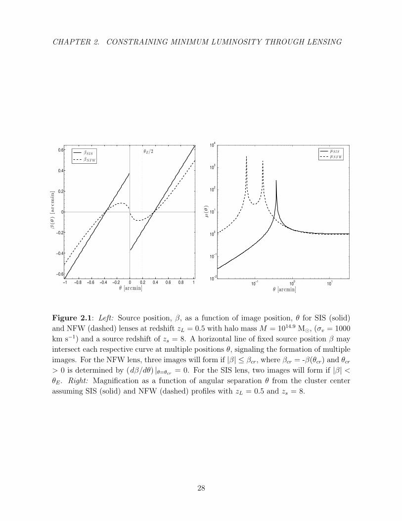
Figure 2.1: Left: Source position, β, as a function of image position, θ for SIS (solid)
and NFW (dashed) lenses at redshift zL = 0.5 with halo mass M = 1014.9 M, (σv = 1000
km s−1) and a source redshift of zs = 8. A horizontal line of fixed source position β may
intersect each respective curve at multiple positions θ, signaling the formation of multiple
images. For the NFW lens, three images will form if |β| ≤ βcr, where βcr = -β(θcr) and θcr> 0 is determined by (dβ/dθ) |θ=θcr = 0. For the SIS lens, two images will form if |β| <θE. Right: Magnification as a function of angular separation θ from the cluster center
assuming SIS (solid) and NFW (dashed) profiles with zL = 0.5 and zs = 8.
28

CHAPTER 2. CONSTRAINING MINIMUM LUMINOSITY THROUGH LENSING
and θvir = rvir/Dl. As can be seen in Figure 2.1, an NFW profile lens will form
three distinct images if |β| ≤ βcr, where βcr = -β(θcr) and θcr > 0 is determined by
(dβ/dθ) |θ=θcr = 0; for all |β| ≥ βcr, a single image is formed.
The equations for κNFW (x) and mNFW (x), used in conjunction with eq. (2.7),
yield the corresponding magnification factor for a NFW profile lens. The two spikes in
µNFW (θ) seen in Figure 2.1 represent the tangential and radial critical curves where the
magnification is formally infinite. The critical curves of the NFW lens are closer to the
lens center than for the SIS lens and the image magnification decreases, approaching
unity, more slowly away from the critical curves.
To model the background galaxy population, we use the Schechter luminosity
function,
φ(z,M)dM = 0.4 ln 10 φ∗(z) 100.4 (α(z)+1)(M∗(z)−M)e−100.4(M∗(z)−M)
(2.21)
where the parameters are the comoving number density of galaxies φ∗, the characteristic
absolute AB magnitude M∗, and the faint-end slope α. (Note that we denote absolute
AB magnitude in this paper as M .) The evolution of φ∗ and M∗ as functions of redshift
in the interval z ≥ 4 are taken as the central values of the fitting formulae provided in
Bouwens et al. (2011b),
φ∗(z) = (1.14± 0.20)× 10−310(0.003±0.055)(z−3.8) Mpc−3 , (2.22)
M∗(z) = (−21.02± 0.09) + (0.33± 0.06)(z − 3.8) . (2.23)
Bouwens et al. (2011b) also provides a fitting formula describing the evolution of α as a
function of redshift,
α(z) = (−1.73± 0.05) + (−0.01± 0.04)(z − 3.8) . (2.24)
29
CHAPTER 2. CONSTRAINING MINIMUM LUMINOSITY THROUGH LENSING
Recent studies have investigated the form of the z = 8 luminosity function by combining
the faint-end results in Bouwens et al. (2011b) with improved constraints at the bright
end (Bradley et al. 2012; Oesch et al. 2012b; McLure et al. 2013; Schenker et al. 2013).
There is very good agreement between the new results, with all studies converging on
a steep faint-end slope of α ' -2.0. We therefore adopt the expression for α(z) in
eq. (2.24) for all redshifts z < 8 and use a faint-end slope of α = -2.02 for all higher
redshifts, assuming that the slope remains unchanged for redshifts z ≥ 8 (McLure et al.
2013). This faint-end slope, along with the formulae describing the evolution of the LF,
represent an extrapolation of the present LF results (z ∼7-8) to even higher redshifts;
the fall-off in UV luminosity at z > 8 is still debated in the literature (Coe et al. 2013;
McLure et al. 2013). The results in this paper may therefore change as the evolution of
the LF parameters φ∗, M∗, and α as functions of redshift are modified in light of new
observations.
In the absence of a lensing object (µ = 1), the number of sources with redshift in
the range zi < z < zf seen in an angular region [θi, θf ] about the optical axis is simply
the number which falls in the angular region with an absolute magnitude less than the
limiting absolute magnitude. This limiting magnitude is set either by the maximum
intrinsic absolute magnitude associated with a star-forming halo, Mmax, or, by what
we denote as Mdet, the absolute magnitude that a source at redshift z must have to
be above df/dν0, the flux threshold set by the detector. This number is thus obtained
by integrating the comoving number density φ(z,M)dM given by eq. (2.21) over the
appropriate volume and magnitude range,
Nunlensed(θi, θf , zi, zf ) = 2π
∫ θf
θi
dθ′θ′dN
dΩ
unlensed
(zi, zf ) (2.25)
30
CHAPTER 2. CONSTRAINING MINIMUM LUMINOSITY THROUGH LENSING
where
dN
dΩ
unlensed
(zi, zf ) =c
H0
∫ zf
zi
dz
E(z)D2s,com(z)
∫ Min[Mmax,Mdet(z)]
−∞dM φ(z,M) . (2.26)
and Dcom is the comoving angular diameter distance, Dcom(z) = DA(1 + z). In the
presence of a lens, the magnification due to gravitational lensing has two effects on
background point sources: their surface number density is diluted by a factor of µ,
nobs(θ) = n/µ(z, θ) , (2.27)
and their luminosities are simultaneously magnified by the same factor,
Lobs(θ) = µ(z, θ)L → Mobs = M + 2.5 log µ(z, θ) . (2.28)
Furthermore, in the case of strong lensing, multiple images will often be produced by SIS
and NFW profile lenses depending on the source position, ~β. When |β| < θE, an SIS lens
will form two images with a splitting angle of ∆θSIS = 2θE. Similarly, an NFW profile
lens will form three distinct images if |β| ≤ βcr; however, only two of those images will
lie in the region |θ| ≥ θE/2 (Figure 2.1), the region of interest in the following section.
In general, the splitting angle ∆θ between these two outside images is insensitive to the
value of β and is approximately given by Li & Ostriker (2002)
∆θNFW ≈ ∆θ(β = 0) = 2θ0, for |β| < βcr (2.29)
where θ0 is the positive root of β(θ) = 0. Consequently, the total number of sources
detected in a lensed field takes the following modified form,
N lensed(θf , zi, zf ) = 2π
∫ ∆θ/2
θE/2
dθ′θ′dN
dΩ
lensed
(θ′, zi, zf )
+ 2π
∫ ∆θ−θE/2
∆θ/2
dθ′θ′ max
[0 ,
dN
dΩ
lensed
(θ′, zi, zf )−dN
dΩ
lensed
(|θ′ −∆θ|, zi, zf )]
+ 2π
∫ θf
∆θ−θE/2dθ′θ′
dN
dΩ
lensed
(θ′, zi, zf ) (2.30)
31
CHAPTER 2. CONSTRAINING MINIMUM LUMINOSITY THROUGH LENSING
where
dN
dΩ
lensed
(θ′, zi, zf ) =c
H0
∫ zf
zi
dz
E(z)D2s,com(z)
1
µ2(z, θ′)
∫ min[Mmax,Mdet(z)+2.5 log µ(z,θ′)]
−∞dM φ(z,M) . (2.31)
2.4 Results
We now apply the general relations discussed above to lensing of background sources by
a lens positioned at a redshift zL = 0.5. This redshift is chosen to be consistent with the
average redshift of the galaxy clusters centered in the six deep fields of the HST Frontier
Fields program. In all the calculations presented below, we take zf = 16 as the upper
bound on the redshift range. Beyond this redshift, zf > 16, the results remain the same
(within a precision of one part in ten-thousand); the numerical results drop by . 4% if
instead we assume the first galaxies formed at zf = 13. Although we focus on the lensing
effect due to galaxy clusters (σv ≈ 1000 km/s), we also include the results obtained when
considering lensing by galaxy groups (σv ≈ 500 km/s). We restrict our attention to the
flux thresholds set by the WFC3 aboard the HST and the NIRCam imager of JWST.
The Frontier Fields program achieves AB ≈ 28.7-29 mag optical (ACS) and NIR (WFC3)
imaging, corresponding to flux limits of df/dν0 ∼ 9-12 nJy for a 5σ detection of a point
source after ∼ 105 s. Medium-deep (mlim ' 29.4 mag) and ultra-deep (mlim ' 31.4 mag)
JWST surveys, (corresponding to a 5σ detection of a point source after 104 and 3.6×10⁵
s of exposure respectively), will detect fluxes as low as ∼ 6 and 1 nJy, respectively.
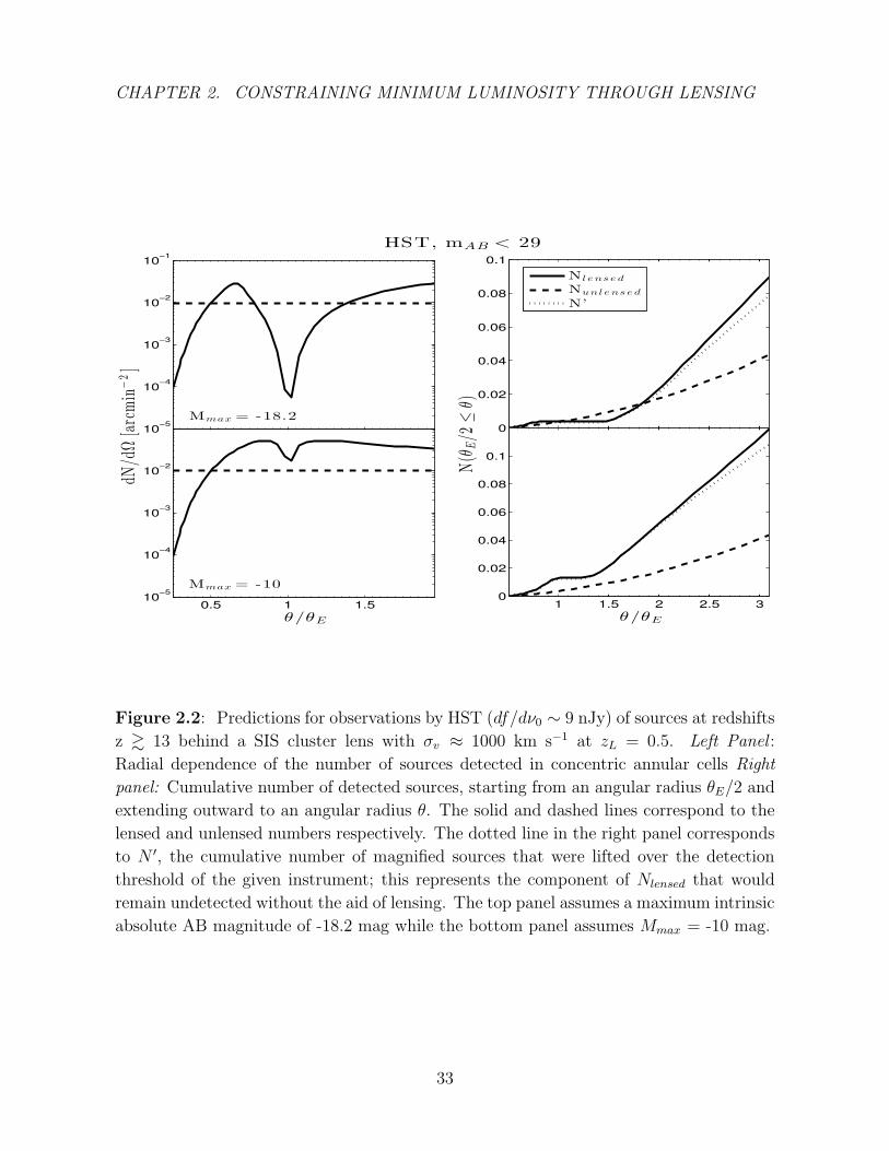
The radial dependence of the number of background sources with redshifts z ≥
13 detected by HST and JWST behind a SIS lens at zL = 0.5 is depicted in the left
panels of Figures 2.2 - 2.4. At large distances from the lens center (θ/θE 1), the
32
CHAPTER 2. CONSTRAINING MINIMUM LUMINOSITY THROUGH LENSING
0
0.02
0.04
0.06
0.08
0.1
Nl e ns e d
Nunl ens e d
N’
1 1.5 2 2.5 30
0.02
0.04
0.06
0.08
0.1
N(θ
E/2
≤θ)
θ/θE0.5 1 1.5
10−5
10−4
10−3
10−2
dN/d
Ω[arcmin
−2]
θ/θE
10−5
10−4
10−3
10−2
10−1
HST, mAB < 29
Mmax = -18.2
Mmax = -10
Figure 2.2: Predictions for observations by HST (df/dν0 ∼ 9 nJy) of sources at redshifts
z & 13 behind a SIS cluster lens with σv ≈ 1000 km s−1 at zL = 0.5. Left Panel :
Radial dependence of the number of sources detected in concentric annular cells Right
panel: Cumulative number of detected sources, starting from an angular radius θE/2 and
extending outward to an angular radius θ. The solid and dashed lines correspond to the
lensed and unlensed numbers respectively. The dotted line in the right panel corresponds
to N ′, the cumulative number of magnified sources that were lifted over the detection
threshold of the given instrument; this represents the component of Nlensed that would
remain undetected without the aid of lensing. The top panel assumes a maximum intrinsic
absolute AB magnitude of -18.2 mag while the bottom panel assumes Mmax = -10 mag.
33
CHAPTER 2. CONSTRAINING MINIMUM LUMINOSITY THROUGH LENSING
0
0.05
0.1
0.15
0.2
Nl e ns e d
Nunl ens e d
N’
1 1.5 2 2.5 30
0.05
0.1
0.15
0.2
0.25
0.3
N(θ
E/2
≤θ)
θ/θE0.5 1 1.5
10−3
10−2
10−1
dN/d
Ω[arcmin
−2]
θ/θE
10−5
10−4
10−3
10−2
10−1
JWST medium-deep, mAB < 29.4
Mmax = -18.2
Mmax = -10
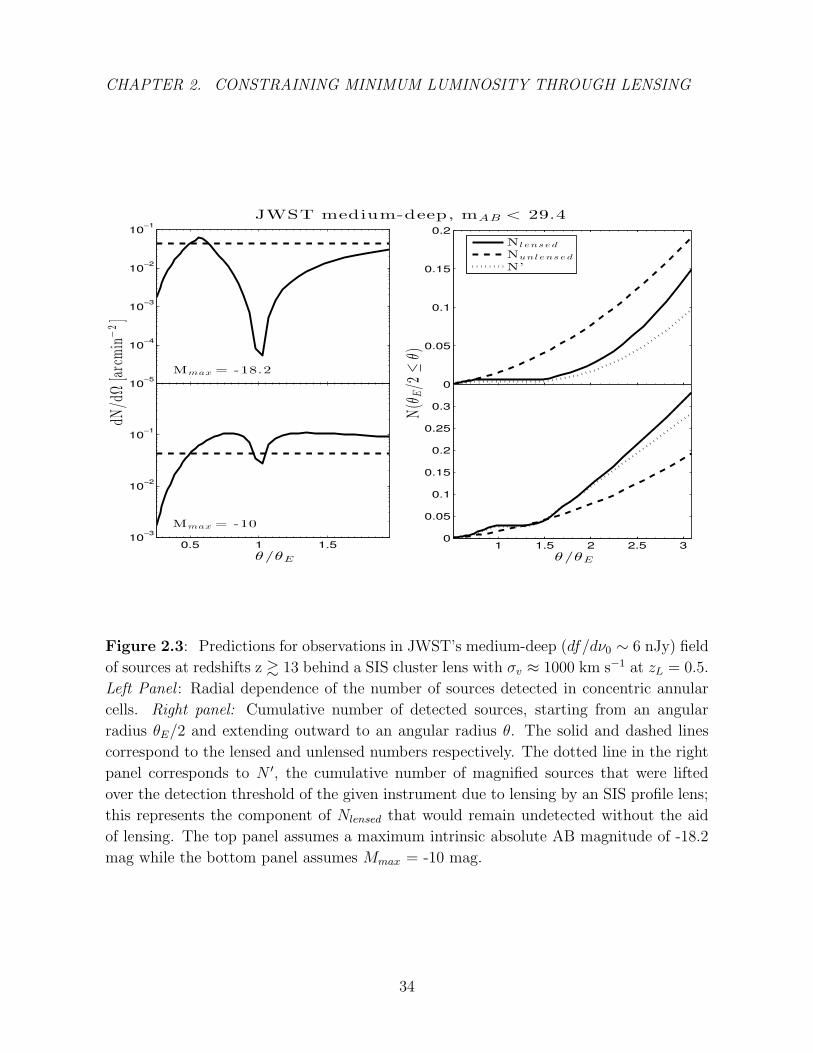
Figure 2.3: Predictions for observations in JWST’s medium-deep (df/dν0 ∼ 6 nJy) field
of sources at redshifts z & 13 behind a SIS cluster lens with σv ≈ 1000 km s−1 at zL = 0.5.
Left Panel : Radial dependence of the number of sources detected in concentric annular
cells. Right panel: Cumulative number of detected sources, starting from an angular
radius θE/2 and extending outward to an angular radius θ. The solid and dashed lines
correspond to the lensed and unlensed numbers respectively. The dotted line in the right
panel corresponds to N ′, the cumulative number of magnified sources that were lifted
over the detection threshold of the given instrument due to lensing by an SIS profile lens;
this represents the component of Nlensed that would remain undetected without the aid
of lensing. The top panel assumes a maximum intrinsic absolute AB magnitude of -18.2
mag while the bottom panel assumes Mmax = -10 mag.
34
CHAPTER 2. CONSTRAINING MINIMUM LUMINOSITY THROUGH LENSING
0
0.1
0.2
0.3
0.4
0.5
0.6
0.7
Nl e ns e d
Nunl ens e d
N’
1 1.5 2 2.5 30
5
10
15N(θ
E/2
≤θ)
θ/θE0.5 1 1.5
10−2
10−1
100
dN/d
Ω[arcmin
−2]
θ/θE
10−6
10−4
10−2
100
102
JWST ultra-deep, mAB < 31.4
Mmax = -18.2
Mmax = -10
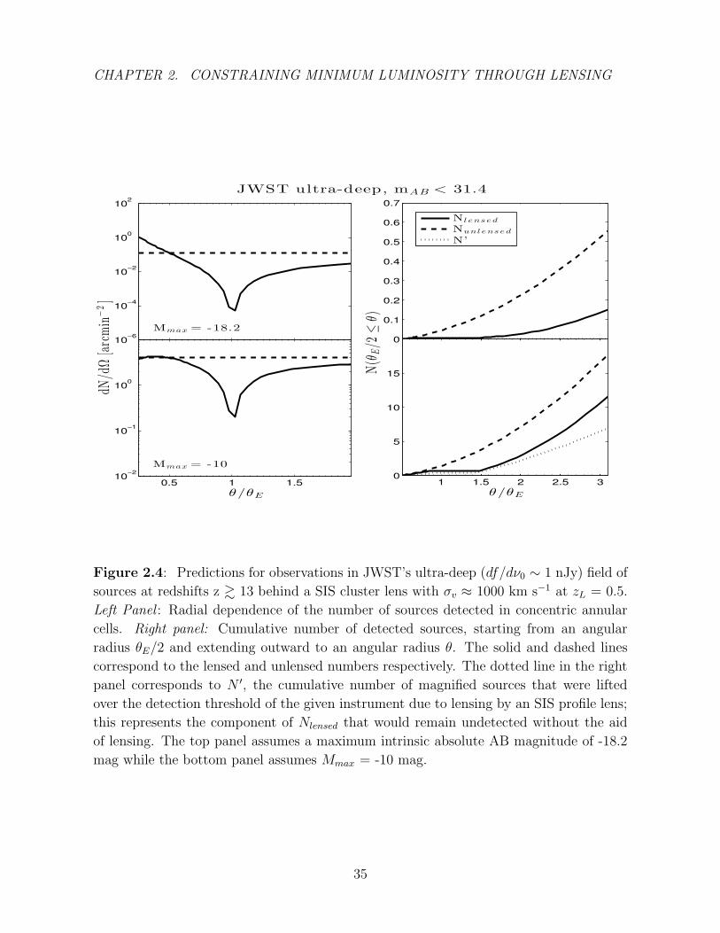
Figure 2.4: Predictions for observations in JWST’s ultra-deep (df/dν0 ∼ 1 nJy) field of
sources at redshifts z & 13 behind a SIS cluster lens with σv ≈ 1000 km s−1 at zL = 0.5.
Left Panel : Radial dependence of the number of sources detected in concentric annular
cells. Right panel: Cumulative number of detected sources, starting from an angular
radius θE/2 and extending outward to an angular radius θ. The solid and dashed lines
correspond to the lensed and unlensed numbers respectively. The dotted line in the right
panel corresponds to N ′, the cumulative number of magnified sources that were lifted
over the detection threshold of the given instrument due to lensing by an SIS profile lens;
this represents the component of Nlensed that would remain undetected without the aid
of lensing. The top panel assumes a maximum intrinsic absolute AB magnitude of -18.2
mag while the bottom panel assumes Mmax = -10 mag.
35
CHAPTER 2. CONSTRAINING MINIMUM LUMINOSITY THROUGH LENSING
magnification factor approaches unity and the number of detected sources per annular
ring converges to the constant number that would be observed in the absence of a
lens (dotted line). For an image at |θ| < θE/2, |µ| is smaller than unity, and the
source luminosity is demagnified relative to the unlensed luminosity while the surface
number density is amplified by the same factor. As θ approaches the Einstein angle,
the magnification diverges, allowing small sources perfectly aligned with the lens center
to form an ”Einstein ring” and otherwise, causing the number density of observed
sources to plummet. (This phenomeneon corresponds to the sharp drop in dN/dΩ at
θ/θE = 1). At image distances larger than the Einstein angle, µ converges back to
unity, resulting in magnified luminosities and diluted number densities that gradually
reduce to their unlensed values. The overall magnification bias depends on which
of the two magnification effects wins out: under circumstances where the number of
magnified sources lifted over the detection threshold outweighs the simultaneous dilution
of the number density of sources in the sky, there is a positive magnification bias and
(dN/dΩ)lensed > (dN/dΩ)unlensed. Conversely, when the reduction in number density
dominates over luminosity magnifications, a negative magnification bias results and
(dN/dΩ)lensed < (dN/dΩ)unlensed in those regions.
The plots of dN/dΩ and N(θE/2 < θ) (the cumulative number of sources observed
starting from an angular radius of θE/2 and extending outward to an angular radius θ) in
Figures 2.2 - 2.4 highlight the sensitivity of the magnification bias to the different model
parameters. The expected magnification bias effect on the source counts observed around
a lensing cluster depends strongly on the flux threshold of the instrument used for the
survey and its strength relative to the characteristic magnitude of the galaxy sample.
If the instrumental detection threshold places the observer in the exponential drop-off
36
CHAPTER 2. CONSTRAINING MINIMUM LUMINOSITY THROUGH LENSING
region of the luminosity function of a galaxy sample, (Mdet(z,fmin) < M∗(z)), lensing
will significantly increase the number of observed sources when it pushes the detection
threshold to fainter values of M , resulting in a positive magnification bias. This is the
case with detections of z ≥ 13 galaxies in HST and medium-deep JWST surveys. On the
other hand, in an ultra-deep JWST survey, where the instrumental limiting magnitude is
fainter than the characteristic magnitude, (placing the observer in the power-law region
of the Schechter function), pushing the threshold to fainter magnitudes does not result in
the inclusion of a substantial population of otherwise undetectable sources; the diluting
effect of lensing therefore wins out and a deficit in the total source count is consistently
observed (Figure 2.4). Source counts of lower redshift galaxy populations in HUDF and
medium-deep JWST surveys suffer from this negative magnification bias as well.
However, note that even in these instances where gravitational lensing reduces the
total source count, a significant fraction of the sources that are observed in the lensed
field belong to a population of galaxies that, without lensing, lie below the survey limit
(dotted lines in right panels of Figures 2.2 - 2.4). By lifting these galaxies over the
instrumental detection threshold, lensing may help constrain another model parameter,
Mmax, the maximum intrinsic absolute magnitude of the background galaxy population.
Figures 2.5 - 2.6 depict the expected source count integrated over the range of
angular distances θ ε [θE/2, 2θE] from the lens center, as a function of the Mmax,
assuming a SIS (solid) and NFW (dashed) profile. Images in this region fall far enough
away from the lens that their detectability is not compromised by the brightness of the
foreground lens, yet close enough that the magnification bias introduced by µ(θ) has a
noticeable effect on the source count. These plots demonstrate that the degree to which
the number count varies as a function of Mmax at the fainter end of the considered range
37

CHAPTER 2. CONSTRAINING MINIMUM LUMINOSITY THROUGH LENSING
0
2
4
6
8
10
σv = 1000 km s−1
NSI S
NNF W
Nunl ens e d
N’
0
5
10
15
−18 −17 −16 −15 −14 −130
50
100
150
200
250
N(θ
E/2<
θ<
2θE)
MAB ,max
−18 −17 −16 −15 −14 −130
5
10
15
N(θ
E/2<
θ<
2θE)
MAB ,max
0
0.5
1
0
0.2
0.4
0.6
0.8
σv = 500 km s−1
HST
JWST ultra-deep
JWST medium-deep
Figure 2.5: Expected number of sources with redshift z & 8 integrated over the region
θE/2 ≤ θ ≤ 2θE as a function of the maximum intrinsic absolute magnitude, MAB,max,
of the background sources.The solid and dashed lines respectively show the expected
numbers due to lensing by a SIS and NFW-profile lens respectively. The dash-dot line
represents the expected numbers in the unlensed case. The dotted line represents the
number of sources in the lensed field that have been lifted over the given instrumental
detection threshold due to lensing by an SIS profile lens. The top, center, and bottom
panels show the expected results given a flux threshold of 9 (HST), 6 (JWST medium-
deep), and 1 nJy (JWST ultra-deep) in the case where galaxy groups (left panel) and
clusters (right panel) are used as lenses with corresponding Einstein angles 0.095’, and
0.38’.
38
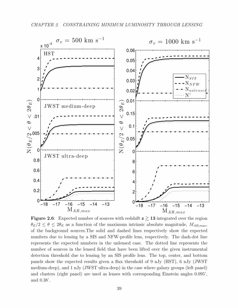
CHAPTER 2. CONSTRAINING MINIMUM LUMINOSITY THROUGH LENSING
0.01
0.02
0.03
0.04
0.05
0.06
σv = 1000 km s−1
NSI S
NNF W
Nunl ens e d
N’
0
0.05
0.1
0.15
−18 −17 −16 −15 −14 −130
2
4
6
8
N(θ
E/2<
θ<
2θE)
MAB ,max
0
1
2
3
4
x 10−3
σv = 500 km s−1
0
.005
.01
−18 −17 −16 −15 −14 −130
0.2
0.4
0.6
0.8
N(θ
E/2<
θ<
2θE)
MAB ,max
JWST ultra-deep
HST
JWST medium-deep
Figure 2.6: Expected number of sources with redshift z & 13 integrated over the region
θE/2 ≤ θ ≤ 2θE as a function of the maximum intrinsic absolute magnitude, MAB,max,
of the background sources.The solid and dashed lines respectively show the expected
numbers due to lensing by a SIS and NFW-profile lens, respectively. The dash-dot line
represents the expected numbers in the unlensed case. The dotted line represents the
number of sources in the lensed field that have been lifted over the given instrumental
detection threshold due to lensing by an SIS profile lens. The top, center, and bottom
panels show the expected results given a flux threshold of 9 nJy (HST), 6 nJy (JWST
medium-deep), and 1 nJy (JWST ultra-deep) in the case where galaxy groups (left panel)
and clusters (right panel) are used as lenses with corresponding Einstein angles 0.095’,
and 0.38’.
39

CHAPTER 2. CONSTRAINING MINIMUM LUMINOSITY THROUGH LENSING
relies significantly on the presence of a magnification bias. In the case of a blank field,
the number count of sources detected by an instrument grows insensitive to Mmax if
this faint-magnitude cut-off is fainter than Mdet; since sources with magnitudes fainter
than Mdet cannot be observed without the aid of gravitational lensing, the unlensed
number count, Nunlensed, plateaus for values of Mmax & Mdet and the presence of these
faint galaxies remains unverifiable. Therefore, an instrument with a flux threshold of ∼9
nJy, such as HST, cannot confirm the existence of sources at redshifts z & 8 and z &
13 with absolute magnitudes fainter than -18.1 and -18.9 mag, respectively. Similarily,
the medium-deep JWST survey loses sensitivity to sources fainter than -17.7 (z ≥ 8)
and -18.5 mag (z ≥ 13) while the ultra-deep survey will not detect sources fainter than
-15.7 (z ≥ 8) and -16.5 mag (z ≥ 13) when observations are made in a blank field.
This sensitivity to the intrinsic faint-magnitude cut-off significantly improves when
considering Nlensed, the number of high-redshift sources one expects to observe behind a
lensing group or cluster. Although the gain in depth does not balance the dilution of
sources in most instances, particularly when observing sources at redshifts z < 13 with
HST and JWST, it permits the detection of sources fainter than Mdet and thus allows
the lensed number count to remain sensitive to Mmax, down to values much fainter than
was the case for the unlensed number count. In particular, the number count of z & 8
galaxies lensed by a foreground cluster modeled as a SIS lens, can be used to infer the
intrinsic faint-magnitude cut-off of the Schecter function up to values as faint as Mmax ∼
-17.8, -17.3, and -15.0 mag (Lmin ∼ 5.8×1027, 3.6×1027, and 4.4×1026 erg s−1Hz−1) in
the HUDF, medium-deep, and ultra-deep JWST surveys, respectively (Figure 2.5, right
panel). Similarly, observations of z & 13 galaxies in ultra-deep JWST surveys can yield
an estimate of Mmax for values as faint as -16.1 mag (Lmin ∼ 1.2×1027) (Figure 2.6, right
40
CHAPTER 2. CONSTRAINING MINIMUM LUMINOSITY THROUGH LENSING
panel). Modeling the cluster as a NFW lens instead results in the same constraints on
Mmax and changes the magnitude of Nlensed by at most ∼ 20% compared to the numbers
obtained for the SIS lens.
Given that the number of galaxies in a field of observation follows a Poisson
distribution and that the sample size is large (which is expected in fields centered on
strong lensing galaxy clusters), the 1-σ confidence interval around the measured count
translates into a range of inferred Lmin values. Using the appropriate plots in Figures 2.5
and 2.6, one can therefore identify the most likely value of Mmax to within the Poisson
uncertainty of the observed number count,√Nobs. An observed number count with an
error bar that lies outside the model, (i.e. Nobs +√Nobs exceeds the maximum number
count accommodated by the model), will subsequently yield only a lower bound on the
intrinsic faint-magnitude cut-off. Figure 2.7 compares the constraint on Mmax that may
be obtained by observing galaxy populations within a given range of redshifts with HST
and JWST in blank versus lensed fields. When observing z ≥ 6 galaxies, the intrinsic
maximum magnitude can be inferred up to values as faint as -14.4 mag (2.5×1026 erg
s−1Hz−1) with JWST.
In addition to constraining the value of Lmin, Figures 2.5 and 2.6 also demonstrate
the instances in which gravitational lensing improves the detection of high redshift
sources as well as the magnitude of the bias in each case. Gravitational lensing by a
group or cluster modeled as an SIS lens reduces the number of detected sources with
redshift z & 8 by a factor of ∼ 2-3 in HST and JWST observations. However, even
though the total source count is reduced in these cases, the majority of the sources
that are observed in the lensed field are galaxies that, without lensing, would remain
undetectable. In particular, nearly ∼ 73-76% of the z ≥ 8 galaxies observed in HUDF
41
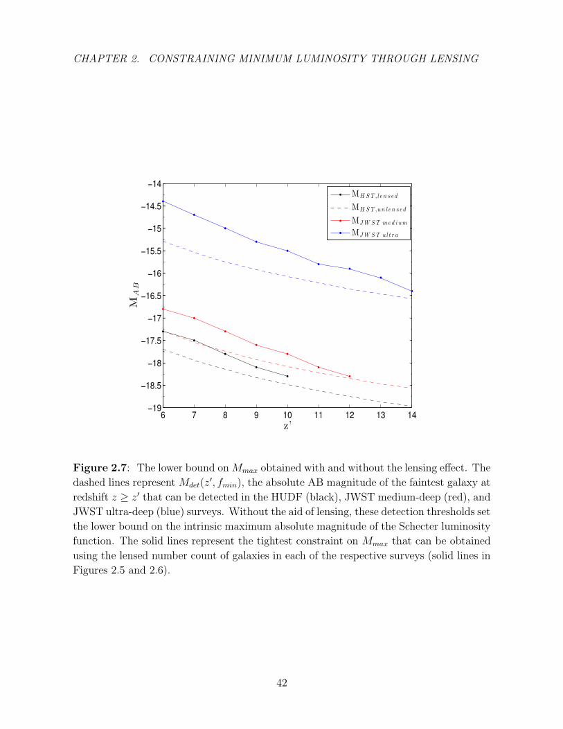
CHAPTER 2. CONSTRAINING MINIMUM LUMINOSITY THROUGH LENSING
6 7 8 9 10 11 12 13 14−19
−18.5
−18
−17.5
−17
−16.5
−16
−15.5
−15
−14.5
−14
z’
MAB
MH S T , len sed
MH S T ,un len sed
MJ W S T med i um
MJ W S T ult r a
Figure 2.7: The lower bound on Mmax obtained with and without the lensing effect. The
dashed lines represent Mdet(z′, fmin), the absolute AB magnitude of the faintest galaxy at
redshift z ≥ z′ that can be detected in the HUDF (black), JWST medium-deep (red), and
JWST ultra-deep (blue) surveys. Without the aid of lensing, these detection thresholds set
the lower bound on the intrinsic maximum absolute magnitude of the Schecter luminosity
function. The solid lines represent the tightest constraint on Mmax that can be obtained
using the lensed number count of galaxies in each of the respective surveys (solid lines in
Figures 2.5 and 2.6).
42
CHAPTER 2. CONSTRAINING MINIMUM LUMINOSITY THROUGH LENSING
and JWST surveys have been lifted over the respective instrumental detection thresholds
(dotted lines). At higher redshifts, the magnification bias transitions from negative to
positive and enhances the number of z & 13 sources detected behind a lensing group or
cluster by a factor of ∼ 3 and 1.5 in HUDF and JWST medium-field surveys, respectively.
Of these observed sources, nearly ∼ 96-98% of them lie below the survey limit and would
thus remain undetected without the aid of gravitational lensing
2.5 Discussion
In this paper, we studied the effects of gravitational lensing on the source count of high
redshift objects as observed by both the HST Frontier Fields and JWST. Although
lensing magnifies the background sources, effectively lowering the flux threshold above
which they can be detected, it simultaneously dilutes the apparent number density
of sources on the sky. We found that the details of whether the number counts of
distant background sources seen through a foreground gravitational lens are enhanced
or reduced depends on several parameters characterizing the system. Using the axially
symmetric SIS and NFW mass density profiles to model a lens residing at a redshift zL
= 0.5, we explored how the magnification bias varied with the velocity dispersion of
the lens (σv), the angular distance from the lens (θ), the photometric sensitivity of the
instrument (df/dν0), the redshift of the background source population, and the intrinsic
faint-magnitude cut-off characterizing the population (Mmax). We found that when
observing sources at redshifts z & 8, lensing by a group or cluster will reduce the number
of detected sources by a factor of ∼ 2-3 in both HST and JWST observations. The
magnification bias transitions from negative to positive only when considering higher
43
CHAPTER 2. CONSTRAINING MINIMUM LUMINOSITY THROUGH LENSING
redshift galaxies; in particular, the bias will enhance the number of sources at redshifts
z & 13 behind a lensing group or cluster by a factor of ∼ 3 and 1.5 in HUDF and JWST
medium-deep surveys, respectively.
Although the gain in depth does not balance the simultaneous dilution of sources
in most instances, it permits the detection of sources fainter than Mdet and thus allows
the lensed number count to remain sensitive to Mmax, down to values much fainter
than was the case for the unlensed number count. In particular, the number count
of z & 8 galaxies lensed by a foreground cluster, can be used to infer the intrinsic
maximum magnitude of the Schecter function up to values as faint as Mmax ∼ -17.8
and -15 mag (Lmin ∼ 5.8×1027 and 4.4×1026 erg s−1Hz−1) in the HUDF and ultra-deep
JWST surveys, respectively, within the range bracketed by existing theoretical models
(Munoz & Loeb 2011; Wyithe & Loeb 2006). Similarly, observations of z & 13 galaxies
in ultra-deep JWST surveys can yield an estimate of Mmax for values as faint as -16.1
mag (Lmin ∼ 1.2×1027 erg s−1Hz−1).
2.6 Acknowledgements
We thank Dan Stark for helpful comments on the manuscript. This work was
supported in part by NSF grant AST-0907890 and NASA grants NNX08AL43G and
NNA09DB30A.This material is based upon work supported by the National Science
Foundation Graduate Research Fellowship under Grant No. DGE1144152. Any opinion,
findings, and conclusions or recommendations expressed in this material are those of the
authors(s) and do not necessarily reflect the views of the National Science Foundation.
44
Chapter 3
An Empirical Model for the Galaxy
Luminosity and Star Formation Rate
Function at High Redshift
This thesis chapter originally appeared in the literature as
N. Mashian, P. A. Oesch, and A. Loeb, An empirical model for
the galaxy luminosity and star formation rate function at high
redshift, Monthly Notices of the Royal Astronomical Society,
455, 2101, 2016
3.1 Abstract
Using the most recent measurements of the ultraviolet (UV) luminosity functions (LFs)
and dust estimates of early galaxies, we derive updated dust-corrected star-formation
45
CHAPTER 3. GALAXY LUMINOSITY AND SFR FUNCTION
rate functions (SFRFs) at z ∼ 4− 8, which we model to predict the evolution to higher
redshifts, z > 8. We employ abundance matching techniques to calibrate a relation
between galaxy star formation rate (SFR) and host halo mass Mh by mapping the shape
of the observed SFRFs at z ∼ 4-8 to that of the halo mass function. The resulting scaling
law remains roughly constant over this redshift range. We apply the average SFR−Mh
relation to reproduce the observed SFR functions at 4 . z . 8 and also derive the
expected UV LFs at higher redshifts. At z ∼ 9 and z ∼ 10 these model LFs are in
excellent agreement with current observed estimates. Our predicted number densities
and UV LFs at z > 10 indicate that JWST will be able to detect galaxies out to z ∼ 15
with an extensive treasury sized program. We also derive the redshift evolution of the
star formation rate density and associated reionization history by galaxies. Models which
integrate down to the current HUDF12/XDF detection limit (MUV ∼ -17.7 mag) result
in a SFRD that declines as (1 + z)−10.4±0.3 at high redshift and fail to reproduce the
observed CMB electron scattering optical depth, τ ' 0.066, to within 1σ. On the other
hand, we find that the inclusion of galaxies with SFRs well below the current detection
limit (MUV < -5.7 mag) leads to a fully reionized universe by z ∼ 6.5 and an optical
depth of τ ' 0.054, consistent with the recently derived Planck value at the 1σ level.
3.2 Introduction
The sensitive, near-infrared imaging capabilities of the Hubble Space Telescope (HST)
have significantly expanded our understanding of galaxy evolution through cosmic time.
Efforts to identify galaxies through photometric selections and follow-up spectroscopy
have progressively extended the observational frontier to higher and higher redshifts,
46

CHAPTER 3. GALAXY LUMINOSITY AND SFR FUNCTION
resulting in robust galaxy samples in the range z ∼ 4-8 (e.g. Madau et al. 1996; Steidel
et al. 1999; Bouwens et al. 2004, 2010, 2011b, 2014b; Dickinson et al. 2004; Yan &
Windhorst 2004a; Bunker et al. 2010; Finkelstein et al. 2010, 2012b,a, 2015; McLure
et al. 2010, 2013; Oesch et al. 2010, 2012b; Schenker et al. 2012, 2013; Bradley et al.
2014; Schmidt et al. 2014). With the Wide Field Camera 3 (WFC3/IR) on board the
HST, the current frontier for identifying high-redshift galaxies now lies at z ∼ 11, a mere
half a billion years after the Big Bang, and new surveys are now building up the sample
sizes of z & 9 galaxies (e.g. Bouwens et al. 2011a; Ellis et al. 2013; Zheng et al. 2012;
Coe et al. 2013; McLure et al. 2013; Oesch et al. 2013, 2014; Bouwens et al. 2014a; Oesch
et al. 2012a; McLeod et al. 2015; Ishigaki et al. 2015).
However, due to the small number statistics, our understanding of galaxies beyond
z ∼ 8 is still very limited and obtaining accurate constraints on the evolution of the
galaxy rest-frame ultraviolet luminosity function (hereafter referred to as the luminosity
function, or UV LF) in the early universe remains challenging. Typically parameterized
by a Schechter function with a power-law slope at faint luminosities and an exponentially
declining form at the bright end, the luminosity function provides a measure of the
relative space density of galaxies over a wide range of luminosities at a particular redshift
(Schechter 1976). Since the UV 1500 A light probes recent star formation activity, the
integral of the dust-corrected (intrinsic) luminosity function can then be used to derive
the cosmic star formation rate density (SFRD) and estimate the galaxy population’s
contribution to cosmic reionization, a process that appears to have been completed by
z ∼ 6 (Finkelstein et al. 2012b; Loeb & Furlanetto 2013; Robertson et al. 2013; Bouwens
et al. 2015b). Given the scarce number of z ∼ 9-10 galaxy candidate detections, a
reliable determination of the SFRD at these redshifts remains difficult, with conclusions
47
CHAPTER 3. GALAXY LUMINOSITY AND SFR FUNCTION
from separate analyses disagreeing on the SFRD evolutionary trends (Coe et al. 2013;
Ellis et al. 2013; Oesch et al. 2013, 2014). Furthermore, with the identification of galaxies
at these redshifts, we are approaching the limit of HST’s detection capabilities. Sources
beyond z ∼ 11 will continue to remain largely inaccessible until the advent of the James
Webb Space Telescope (JWST), whose scheduled launch in 2018 promises to yield
revolutionary insights into early galaxy formation at z > 10 (Gardner et al. 2006).
The analysis and extrapolation of the UV luminosity function evolution towards
higher (z ≈ 8) redshifts has been the focus of several past studies, in the form of both
hydrodynamical simulations (e.g. Nagamine et al. 2010; Finlator et al. 2011a; Salvaterra
et al. 2011; Jaacks et al. 2012; Dayal et al. 2013; O’Shea et al. 2015) and semi-analytical
models (e.g. Trenti et al. 2010; Munoz 2012; Tacchella et al. 2013; Cai et al. 2014; Dayal
et al. 2014; Behroozi & Silk 2015). Successfully reproducing the statistical properties of
the observed Lyman-break galaxy (LBG) population at z = 6-9, simulations predict a
large number of undetected, low-mass galaxies that may have significantly contributed
to the reionization of the Universe at z ≥ 6. Semi-empirical models which tie the
evolution of galaxy luminosity to the dark matter properties of the host halos reach
similar conclusions, predicting a steepening faint-end slope of the LF with redshift and
a sharp decline in the cosmic star formation rate above z =8 (Mason et al. 2015; Trac
et al. 2015).
In this paper, we take advantage of the recent progress in the observed galaxy
statistics at redshifts z ∼ 4-8 to evolve the luminosity function, along with its derived
properties, towards higher redshifts by establishing a link between the galaxy star
formation rate (SFR) and its host halo mass via abundance matching techniques (Vale
& Ostriker 2004, 2006; Conroy & Wechsler 2009). Since galaxy formation is governed
48
CHAPTER 3. GALAXY LUMINOSITY AND SFR FUNCTION
by the inflow of baryonic matter into the gravitational potential wells of dark matter
halos where it cools and initiates star formation, the properties of galaxies are invariably
linked to the characteristics of their host halos. We thus seek to derive a scaling relation
between dark matter halo mass, Mh and galaxy SFR at each redshift by assuming
that there is a one-to-one, monotonic correspondence between these two properties.
We anchor our model to the observed luminosity functions at z ∼ 4-8 corrected for
dust-extinction, mapping their shape to that of the halo mass function at the respective
redshifts. Finding that the SFR-Mh scaling law remains roughly constant across this
redshift range, we apply the average relation, SFRav(Mh), to reproduce the observed
z ∼ 9-10 luminosity functions and then further explore how the UV LF, and the
corresponding SFRD, evolve at higher redshifts, z ∼ 11-20.
We describe the details of our approach and the theoretical framework used to
derive the shape and amplitude of the galaxy UV LF in section 3.3. Our predictions for
the evolving LF, the resulting SFRD, and the contribution of these galaxy populations
to cosmic reionization at high redshifts are presented in section 3.4. We conclude in
section 3.5 with a summary of our findings and their implications for future surveys with
JWST. We adopt a flat, ΛCDM cosmology with Ωm = 0.3, ΩΛ = 0.7, Ωb = 0.045, H0 =
70 km s−1Mpc−1, i.e. h = 0.7, σ8 = 0.82, and ns = 0.95, consistent with the most recent
measurements from Planck (Planck Collaboration et al. 2016b). All magnitudes in this
work are in the AB scale (Oke & Gunn 1983).
49

CHAPTER 3. GALAXY LUMINOSITY AND SFR FUNCTION
3.3 The Formalism
The goal of this paper is to derive an empirical prediction of the evolution of UV LFs
at z > 8 tied to the evolution of dark matter haloes. We do so by first calibrating a
SFR −Mh relation at z ∼ 4 − 8, which we then evolve to z > 8. Our formalism is
described in the following sections.
3.3.1 The Observed Star-Formation Rate Functions
One important limitation of the UV LFs in probing the galaxy build-up in the early
universe is dust extinction, which significantly affects the UV luminosities of galaxies.
Thanks to deep multi-wavelength photometry with HST, it has become clear that dust
extinction evolves with redshift, becoming significantly less important at earlier cosmic
times (Bouwens et al. 2009a; Castellano et al. 2012; Finkelstein et al. 2012b; Dunlop
et al. 2013; Bouwens et al. 2014b; Rogers et al. 2014). Thus, the UV LF at high redshift
evolves due to two effects: (i) evolution in dust extinction, and (ii) SFR build-up of the
underlying galaxy population. Any model of the UV LFs therefore has to disentangle
these two effects.
Alternatively, we can directly make use of the SFR functions (SFRF), φ(SFR, z).
These provide the number density of galaxies with a given SFR, and are thus corrected
for dust extinction. Following Smit et al. (2012), we derive the observed SFR functions
based on the most recent UV LFs at z > 4 taken from Bouwens et al. (2015b), which we
correct for dust extinction using the observed UV continuum slopes β and their relation
with UV extinction (Meurer et al. 1999). The UV continuum slopes are modeled as a
50
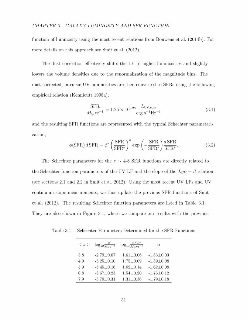
CHAPTER 3. GALAXY LUMINOSITY AND SFR FUNCTION
function of luminosity using the most recent relations from Bouwens et al. (2014b). For
more details on this approach see Smit et al. (2012).
The dust correction effectively shifts the LF to higher luminosities and slightly
lowers the volume densities due to the renormalization of the magnitude bins. The
dust-corrected, intrinsic UV luminosities are then converted to SFRs using the following
empirical relation (Kennicutt 1998a),
SFR
M yr−1 = 1.25× 10⁻²⁸ LUV,corr
erg s−1Hz−1 (3.1)
and the resulting SFR functions are represented with the typical Schechter parameteri-
zation,
φ(SFR) d SFR = φ∗(
SFR
SFR∗
)αexp
(− SFR
SFR∗
)d SFR
SFR∗. (3.2)
The Schechter parameters for the z ∼ 4-8 SFR functions are directly related to
the Schechter function parameters of the UV LF and the slope of the LUV − β relation
(see sections 2.1 and 2.2 in Smit et al. 2012). Using the most recent UV LFs and UV
continuum slope measurements, we thus update the previous SFR functions of Smit
et al. (2012). The resulting Schechter function parameters are listed in Table 3.1.
They are also shown in Figure 3.1, where we compare our results with the previous
Table 3.1. Schechter Parameters Determined for the SFR Functions
< z > log10φ∗
Mpc−3 log10SFR∗
Myr−1 α
3.8 -2.79±0.07 1.61±0.06 -1.53±0.03
4.9 -3.25±0.10 1.75±0.09 -1.59±0.08
5.9 -3.45±0.16 1.62±0.14 -1.62±0.08
6.8 -3.67±0.23 1.54±0.20 -1.76±0.12
7.9 -3.79±0.31 1.31±0.36 -1.79±0.18
51
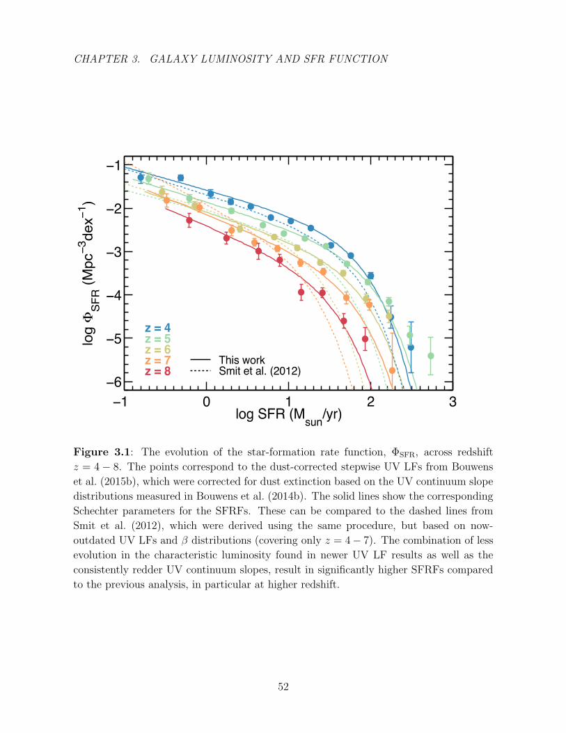
CHAPTER 3. GALAXY LUMINOSITY AND SFR FUNCTION
−1 0 1 2 3−6
−5
−4
−3
−2
−1
log SFR (Msun/yr)
log \SF
R (M
pc−3dex−1 )
z = 4z = 5z = 6z = 7z = 8
This workSmit et al. (2012)
Figure 3.1: The evolution of the star-formation rate function, ΦSFR, across redshift
z = 4 − 8. The points correspond to the dust-corrected stepwise UV LFs from Bouwens
et al. (2015b), which were corrected for dust extinction based on the UV continuum slope
distributions measured in Bouwens et al. (2014b). The solid lines show the corresponding
Schechter parameters for the SFRFs. These can be compared to the dashed lines from
Smit et al. (2012), which were derived using the same procedure, but based on now-
outdated UV LFs and β distributions (covering only z = 4− 7). The combination of less
evolution in the characteristic luminosity found in newer UV LF results as well as the
consistently redder UV continuum slopes, result in significantly higher SFRFs compared
to the previous analysis, in particular at higher redshift.
52

CHAPTER 3. GALAXY LUMINOSITY AND SFR FUNCTION
analysis of Smit et al. (2012). As can be seen, the combination of less evolution in the
characteristic luminosity found in newer UV LF results, as well as the consistently redder
UV continuum slopes found in updated measurements, result in significantly higher
SFRFs compared to the previous analysis, in particular at higher redshift.
We perform the same analysis also for z ∼ 9− 10 galaxy SFR functions. These are
much more uncertain, given the very large uncertainties in the UV LFs at these redshifts.
Also, note that based on the evolution of the UV continuum slope distribution at lower
redshift (Bouwens et al. 2012b, 2014b; Dunlop et al. 2013; Finkelstein et al. 2012b;
Wilkins et al. 2011), the dust correction is expected to be negligible at redshifts z > 8;
the z ∼ 9 and 10 SFR function parameters are thus directly related to the uncorrected
UV LFs at those redshifts.
3.3.2 Method to derive the average SFR−Mh relation
Adopting the approach presented in Vale & Ostriker (2004), we use the observed,
dust-corrected z ∼ 4-8 luminosity functions, i.e. SFR functions, to derive an empirical
relation between the galaxy SFR and its host halo mass. In this abundance matching
method, the SFR-Mh relation is calculated by setting the SFR of a galaxy hosted in
a halo of mass Mh to be such that the number of galaxies with a star formation rate
greater than SFR equals the number of halos with mass greater than Mh at a given
epoch: ∫ ∞Mh
n(M ′h, z)dM ′
h =
∫ ∞SFR
φ(SFR’, z)dSFR’, (3.3)
53

CHAPTER 3. GALAXY LUMINOSITY AND SFR FUNCTION
where the φ(SFR, z) are the observed SFR function derived in the previous section and
n(Mh, z) is the Sheth-Tormen halo mass function (Sheth & Tormen 1999),
n(Mh, z)dM = A
(1 +
1
ν2q
)√2
π
ρmM
dν
dMe−ν
2/2 (3.4)
with ν =√aδc/[D(z)σ(M)], a = 0.707, A = 0.322 and q = 0.3; σ(M) is the variance on
the mass scale M (assuming the linear theory density power spectrum) while D(z) is the
growth favor and δc is the linear threshold for spherical collapse, which in a flat universe
is δc = 1.686.
The abundance matching technique, as prescribed in eq. (3.3), presupposes that
the SFR is a monotonic function of the halo mass. This is supported by the observed
trend that the clustering strength of galaxies at high redshift increases with their UV
luminosity, similar to that of the clustering strength of halos increasing with mass
(Lee et al. 2009). Hence, a scaling relation that assumes the SFR of a galaxy is a
monotonically increasing function of the mass of its host halo is a reasonable starting
point. Furthermore, our model assumes a one-to-one correspondence between galaxies
and host halos. This neglects the substructure expected to exist within a halo, comprised
mainly of halos that formed at earlier epochs and merged to become subhaloes of more
massive hosts (Bullock et al. 2002; Wechsler et al. 2000). To include the contribution
of this subhalo population and the galaxies they are potentially hosting, we modified
the left-hand side of eq. (3.3) to integrate over the total mass function, i.e. the sum of
the regular Sheth-Tormen halo mass function and the unevolved subhalo mass function
taken from Vale & Ostriker (2004). We found that because values for the subhalo mass
function are generally lower than those of the halo mass function, the inclusion of this
additional substructure has a negligible effect on the resulting scaling law; the subhaloes’
54
CHAPTER 3. GALAXY LUMINOSITY AND SFR FUNCTION
contribution to the expression is most important at the low-mass end, and even there, its
inclusion changes the results by . 10%. Therefore, for the sake of simplicity, we neglect
multiple halo occupation and assume that each dark-matter halo hosts a single galaxy.
3.3.3 Modeling the SFR Functions
Once the average relation between the SFR and the halo mass are known, we can model
the SFR functions assuming a realistic dispersion around the average relation. We model
the probability density for a halo of mass Mh to host a galaxy with a star formation rate
SFR to obey a log-normal distribution (Giavalisco & Dickinson 2001; Yang et al. 2003;
Munoz & Loeb 2011),
P (SFR|Mh)d SFR =1
σ√
2πexp
(− log2
10(SFR/SFRav(Mh))
2σ2
)d log10 SFR (3.5)
where SFRav(Mh) is the mean SFR-Mh relation derived by averaging the SFR(Mh, z)
relations obtained for 4 ≤ z ≤ 8 over the specified range of redshifts at fixed halo mass.
The variance, σ2, represents the scatter in SFR at a fixed Mh that arises from the
stochastic nature of star formation activity. Halos of similar masses can have a range of
large-scale environments, merger histories, and central concentrations (Lee et al. 2009).
These conditions, along with interactions with nearby systems can result in different
rates of gas accretion and star formation in galaxies. To account for this variance in
the SFR-Mh relation, we adopt a constant intrinsic scatter of 0.5 dex. This choice is
motivated by the 0.5 dex scatter in stellar mass at constant SFR found by Gonzalez
et al. (2011), a result further confirmed by Wyithe et al. (2014) as providing the best
statistical fit to observations of the SFR-Mh relation.
The SFR function, φ(SFR), can then be obtained by integrating over the
55
CHAPTER 3. GALAXY LUMINOSITY AND SFR FUNCTION
probability-weighted number densities of all halos that can achieve the star formation
rate SFR within the allowed scatter:
φ(SFR, z) =
∫dMh n(Mh, z)P (SFR|Mh) (3.6)
=1
σ√
2π
1
SFR
∫dMh n(Mh, z) e−
log210(SFR/SFRav(Mh))
2σ2 .
Note that in the limit of the variance σ2 → 0, the log-normal probability distribution
becomes a delta function and the equation is reduced to the simpler form,
φ(SFR, z) = n(Mh, z)
∣∣∣∣∣d SFRav(Mh)
dMh
∣∣∣∣∣−1
. (3.7)
3.4 Results
3.4.1 The Constant SFR−Mh Relation
The curves in the top panel of Figure 3.2 depict the SFR-Mh relations inferred from the
observed LF functions at redshifts 4 ≤ z ≤ 8 via the abundance matching technique
discussed in Section 3.3. The scaling law remains roughly constant within 0.2 dex across
this redshift range and is fairly well fit by a double power law with a turnover at a
characteristic halo mass of M∗h ≈ 2×10¹¹ M. Averaging the relations over z ∼ 4-8
at a fixed halo mass, we obtain a mean scaling law, SFRav(Mh) (solid black curve),
characterized by a power-law slope β ∼ 0.9 at the high-mass end, i.e. Mh & M∗h , and
β ∼ 1.5 at the faint end where Mh falls below the characteristic mass.
These results are consistent with the models presented in Trenti et al. (2010) where
the L −Mh relation is calibrated at z ∼ 6 and a L ∼ Mβh relation is derived with β ∼
1.3-1.6 at the low-mass end. This steepening of the SFR-Mh relation towards lower
56
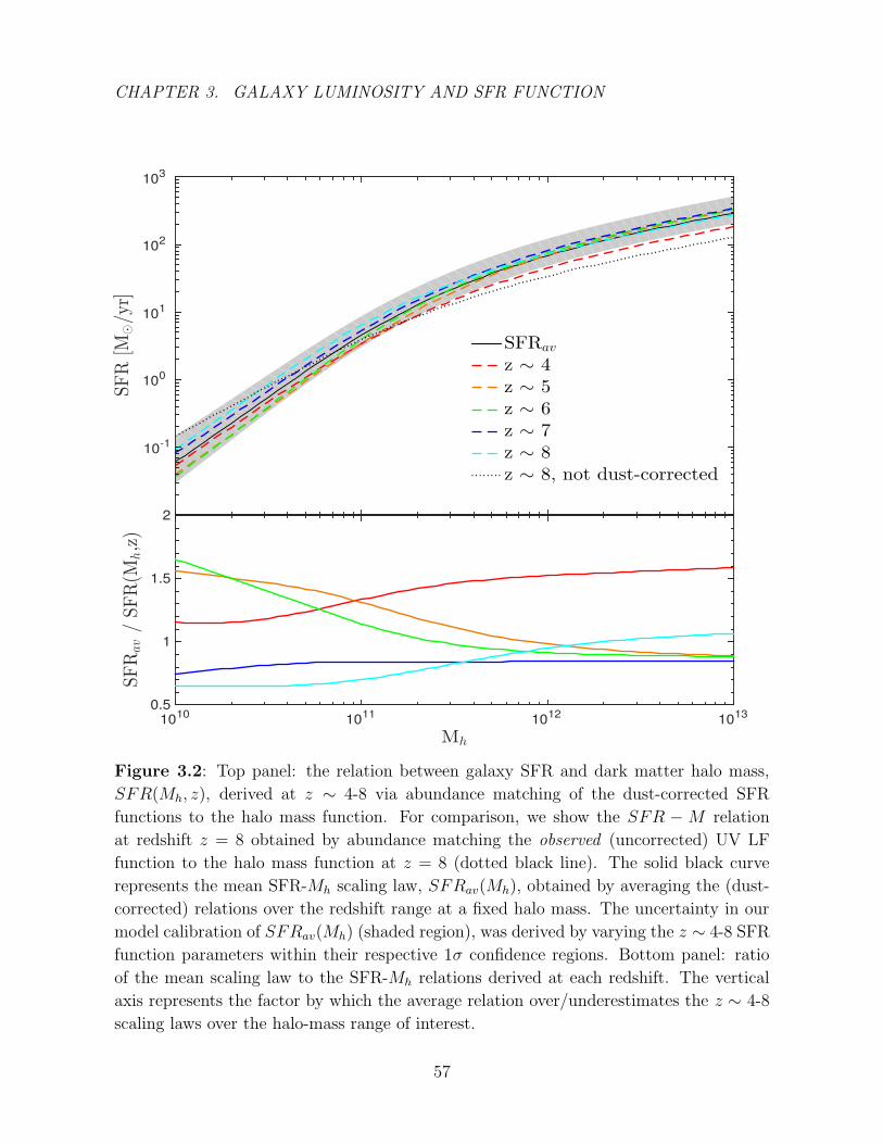
CHAPTER 3. GALAXY LUMINOSITY AND SFR FUNCTION
SFR
[M⊙/y
r]
10-1
100
101
102
103
SFRav
z ∼ 4z ∼ 5z ∼ 6z ∼ 7z ∼ 8z ∼ 8, not dust-corrected
Mh
1010
1011
1012
1013
0.5
1
1.5
2
SFR
av/SFR(M
h,z)
Figure 3.2: Top panel: the relation between galaxy SFR and dark matter halo mass,
SFR(Mh, z), derived at z ∼ 4-8 via abundance matching of the dust-corrected SFR
functions to the halo mass function. For comparison, we show the SFR −M relation
at redshift z = 8 obtained by abundance matching the observed (uncorrected) UV LF
function to the halo mass function at z = 8 (dotted black line). The solid black curve
represents the mean SFR-Mh scaling law, SFRav(Mh), obtained by averaging the (dust-
corrected) relations over the redshift range at a fixed halo mass. The uncertainty in our
model calibration of SFRav(Mh) (shaded region), was derived by varying the z ∼ 4-8 SFR
function parameters within their respective 1σ confidence regions. Bottom panel: ratio
of the mean scaling law to the SFR-Mh relations derived at each redshift. The vertical
axis represents the factor by which the average relation over/underestimates the z ∼ 4-8
scaling laws over the halo-mass range of interest.
57

CHAPTER 3. GALAXY LUMINOSITY AND SFR FUNCTION
masses may be due to the increased importance of feedback mechanisms in the star
formation activity, such as supernovae and stellar winds (Giavalisco & Dickinson 2001).
Meanwhile, the overall flattening of SFR(Mh) at these redshifts compared to the local
universe, where SFR ∝ M4h is mainly a consequence of the steepening faint-end slope of
the observed LF at these redshifts, where α < -1.5 (Cooray & Milosavljevic 2005).
The uncertainty in our model calibration of SFRav(Mh), represented by the shaded
region in Figure 3.2, is derived by varying the z ∼ 4-8 SFR function parameters within
their respective 1σ confidence regions and rederiving the average SFR-Mh relation. As
can be seen, the dashed curves defining the SFR-Mh relation at each redshift fall well
within the boundaries of the uncertainty in the average scaling law, with the exception
of the z ∼ 4 relation at the high-mass end. The bottom panel of Figure 3.2 illustrates
the accuracy with which the mean scaling law approximates SFR as a function of halo
mass at different redshifts. Overall, the SFRav(Mh) relation provides a reasonable
representation of the SFR(Mh, z) relations at all redshifts, with departures of less than
0.2 dex within the halo mass range of interest. With the exception of the z ∼ 4 relation,
the SFR(Mh, z) are all very similar (within 0.5 dex) at Mh > 1012 M. At the low-mass
end, the z ∼ 5-6 and z ∼ 7-8 scaling laws are over- and under-estimated respectively by
less than a factor of two, while the SFR at z ∼ 4 is overestimated over the full halo-mass
range by approximately the same factor. We therefore expect the mean relation to yield
accurate estimates of the SFR function at these redshifts and, assuming that the SFR-Mh
relationship continues to remain roughly unchanged for z > 8, at higher redshifts as well.
58

CHAPTER 3. GALAXY LUMINOSITY AND SFR FUNCTION
3.4.2 The Modeled SFR Functions at z = 4− 8
Applying SFRav(Mh), we derive the expected SFR functions at redshifts z & 4 assuming
only evolution of the underlying dark-matter halo mass function. The results of our
LF model are shown in Figure 3.3, both for the case where an intrinsic scatter of σ ∼
0.5 dex is assumed (solid colored curves) and in the limiting case where the variance is
set to zero (dashed curves). Plotted alongside these results are the dust-corrected data
points and the Schechter LFs with the observed best-fit parameters reported in Table 3.1
(gray curves). We find that including an intrinsic scatter increases the number density
and yields SFR functions that are more consistent with observation, particularly at the
luminous end where the increase in φ(SFR) due to scatter is most apparent. This boost
in number density with the introduction of scatter can be attributed to the shape of
the halo mass function. Even though SFR(Mh) is log-normally distributed around the
mean, SFRav(Mh), and the SFR scatter can thus go in either direction, the net change
in the LF will always be dominated by low-mass halos entering into the galaxy sample
by scattering into a SFR higher than its mean value, leading to a larger estimate of
φ(SFR).
With the exception of z ∼ 4, our predicted SFR functions accurately reproduce
the observed ones and provide very good fits to the data points at the luminous end
when intrinsic scatter is accounted for. At z ∼ 4 our model predicts a SFRF which lies
significantly above the observed data points by factors of 2-10×. This is likely due to a
combination of two effects: (i) As also argued by Smit et al. (2012), the bright end of the
observed z ∼ 4 SFRF is likely underestimated due to heavily obscured galaxies, which
are missed in UV-selected Lyman break galaxy samples; and (ii) quiescent galaxies start
59
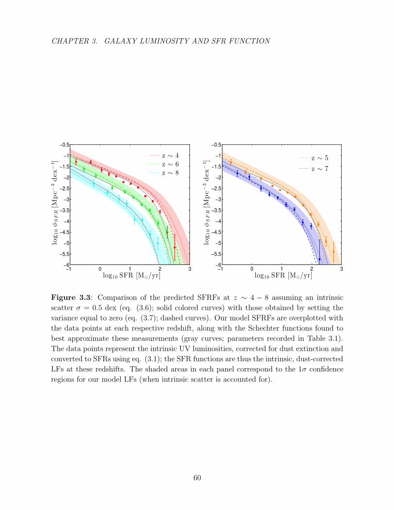
CHAPTER 3. GALAXY LUMINOSITY AND SFR FUNCTION
log10φSFR[M
pc−3dex−1 ]
log10 SFR [M⊙/yr]−1 0 1 2 3
−6
−5.5
−5
−4.5
−4
−3.5
−3
−2.5
−2
−1.5
−1
−0.5
z ∼ 4z ∼ 6z ∼ 8
log10φSFR[M
pc−3dex−1]
log10 SFR [M⊙/yr]−1 0 1 2 3
−6
−5.5
−5
−4.5
−4
−3.5
−3
−2.5
−2
−1.5
−1
−0.5
z ∼ 5
z ∼ 7
Figure 3.3: Comparison of the predicted SFRFs at z ∼ 4 − 8 assuming an intrinsic
scatter σ = 0.5 dex (eq. (3.6); solid colored curves) with those obtained by setting the
variance equal to zero (eq. (3.7); dashed curves). Our model SFRFs are overplotted with
the data points at each respective redshift, along with the Schechter functions found to
best approximate these measurements (gray curves; parameters recorded in Table 3.1).
The data points represent the intrinsic UV luminosities, corrected for dust extinction and
converted to SFRs using eq. (3.1); the SFR functions are thus the intrinsic, dust-corrected
LFs at these redshifts. The shaded areas in each panel correspond to the 1σ confidence
regions for our model LFs (when intrinsic scatter is accounted for).
60

CHAPTER 3. GALAXY LUMINOSITY AND SFR FUNCTION
to appear in the Universe at z ∼ 4 in significant numbers (e.g. Straatman et al. 2014).
Since our model does not include any prescription to quench star formation in galaxies,
this is likely another reason why the model appears to be inadequate at z ∼ 4. We
conclude that our model should only be used at z > 4, where it provides a very good
representation of the observed SFRFs.
3.4.3 A Prediction for the UV LF at z = 9− 10
Building on the successful calibration of the SFR-Mh relation at z ∼ 5 − 8, we use our
model to predict the galaxy UV luminosity function at z ∼ 9 − 10. This represents the
most distant galaxies in reach with HST, and recent observations have started to provide
the first LF estimates at these redshifts. However, the sample sizes are still very small
resulting in highly uncertain LF parameters (see e.g. Oesch et al. 2013).
We derive the model UV LFs at z = 9 and 10 by converting the SFR-Mh relation
calibrated in the previous section to a LUV −Mh relation using the standard Kennicutt
(1998a) SFR-LUV relations. As can be seen in Figure 3.4, our model provides an excellent
fit to the current, albeit scarce, data. In particular, our model explains the somewhat
puzzling absence of z ∼ 10 galaxy candidates between MUV = −18.5 and −20.5 in
current datasets. Incoming observations of the Hubble Frontier Field initiative will allow
us to test this model further at z ∼ 9− 10 in the future.
61

CHAPTER 3. GALAXY LUMINOSITY AND SFR FUNCTION
↓–
↓–
φ(M)[m
ag−1Mpc−3]
MU V
−22 −21 −20 −19 −18 −1710
−7
10−6
10−5
10−4
10−3
10−2
10−1
Oesch+13Bouwens+15
z ∼ 9
↓↓
↓
↓↓
––
––
–
↓–
φ(M)[m
ag−1Mpc−3]
MU V
−22 −21 −20 −19 −18 −1710
−8
10−7
10−6
10−5
10−4
10−3
10−2
Oesch+14Bouwens+15
z ∼ 10
Figure 3.4: Comparison of the predicted LFs assuming an intrinsic scatter σ = 0.5 dex
(eq. (3.6); solid colored curves) with those obtained by setting the variance equal to zero
(eq. (3.7); dashed curves). Since at z ∼ 9 and 10, the dust extinction is expected to be
negligible, the curves represent the observed, uncorrected LFs. We include determinations
of the z ∼ 9 and z ∼ 10 UV LFs from Oesch et al. (2013), Oesch et al. (2014), and Bouwens
et al. (2016). Arrows signify upper bounds on the number density at a given absolute UV
magnitude, MUV . The shaded area in each panel represents the 1σ confidence region for
the model LF when intrinsic scatter is accounted for. Our model UV LFs are in excellent
agreement with the current observed estimates at these redshifts (albeit the latter are still
based on small samples).
62
CHAPTER 3. GALAXY LUMINOSITY AND SFR FUNCTION
3.4.4 Extrapolation to z ∼ 20 and Predictions for JWST
Motivated by the good agreement obtained by applying an unevolving SFR-Mh relation
to reproduce the observed LFs at 5 . z . 10, we extend our approach to even
higher redshifts for JWST predictions. The predicted LFs for redshifts z > 10, again
assuming a constant intrinsic scatter of σ = 0.5 dex, are shown in Figure 3.5. These
model LFs, which are well-fitted by Schechter functions across the redshift range 4
. z . 20, significantly evolve with redshift. The drop in number density from z ∼
4 to 20 is reflected in the evolution of the characteristic number density, φ∗, which
decrease as d log φ∗/dz ∼ -0.3. We also find a gradual steepening of the faint-end slope
(dα/dz ∼ −0.08) and a shifting of the characteristic luminosity towards fainter values
for increasing redshift (dM∗UV /dz ∼ 0.4). These trends in Schechter parameters are quite
consistent with results from previous studies and extrapolations of observed z . 10 LFs,
except that our model M∗ evolves more significantly than found in observations (e.g.,
Trenti et al. 2010; Bouwens et al. 2011b, 2012b; McLure et al. 2013; Finkelstein et al.
2015).
The shaded region in Figure 3.5 corresponds to the comoving volume and magnitude
range accessible with a 200 arcmin2 treasury sized ultra-deep JWST survey (mlim ' 31.5
mag). According to our model predictions, the limiting redshift for galaxy observations
with a very deep JWST survey is z ∼ 15 (see also Windhorst et al. 2006). At higher
redshifts, where the surface density drops below ∼10−6 Mpc−3, wider, deeper surveys
would be required to observe the luminosity function of these rare, faint objects.
Figure 3.6 shows the model predictions for the redshift evolution of the SFR density,
obtained by integrating the SFR functions down to different SFR limits, ranging from
63

CHAPTER 3. GALAXY LUMINOSITY AND SFR FUNCTION
z 911
z 912
z 913 z 9
14z 9
15z 9
16
z 917
z 918
z9
19
z9
20
mUV
27 28 29 30 31 32 33 34
?(m
)[m
ag!
1M
pc!
3]
10-9
10-8
10-7
10-6
10-5
10-4
10-3
Figure 3.5: Predicted LFs for z > 10 based on our empirical model. The shaded region
indicates the observable magnitude and volume within reach of a 200 arcmin2 JWST
treasury sized ultra-deep survey (mlim ' 31.5 mag). This indicates that the limiting
redshift range observable with JWST may be z ∼ 15 for unlensed galaxies.
64

CHAPTER 3. GALAXY LUMINOSITY AND SFR FUNCTION
SFRmin ∼ 10−5 M/yr to 0.7 M/yr. A minimum SFR of 0.7 M/yr corresponds to
MUV ∼ -17.7 mag, the magnitude of the faintest object observed in the HUDF12/XDF
data; integrating down to this limit thus facilities comparison with the most recent,
dust-corrected measurements of the SFRD, which have been plotted alongside the
predicted curves in Figure 3.6. While our model appears to overpredict the SFRD
measured for z . 6 by ∼ 0.2-0.3 dex, the estimates of the ρ∗ at higher redshifts agree
quite well with observations. Furthermore, the evolution of the cosmic SFRD in our
model is consistent with previous published results: the dust-corrected SFRD values
evolve as (1 + z)−4.3±0.1 at 3 < z < 8 before rapidly declining at higher redshifts where
ρ∗ ∝ (1 + z)−10.4±0.3 for 8 ≤ z ≤ 10. In addition to accurately reproducing the order of
magnitude drop in SFRD from z < 8 to z < 10 that has been observationally inferred in
several separate analyses (Oesch et al. 2013), our model finds that the SFRD continues
to steeply decline towards higher redshift, predicting a cosmic SFRD of log ρ∗ ∼ -7.0±0.3
M yr−1Mpc−3 at z ∼ 16.
However, as will be shown and discussed in the following section, a star-formation
rate density that declines as (1+z)−10.4 at high redshifts, as derived assuming a minimum
SFR of 0.7 M/yr, fails to reproduce the observed Planck optical depth. Furthermore,
galaxies are expected to exist beyond the current, observed magnitude limit. Theoretical
and numerical investigations indicate that a halo at z ≤ 10 irradiated by a UV field
comparable to the one required for reionization needs a minimum mass of Mh ∼ 6×10⁷
M in order to cool and form stars (Haiman et al. 1996; Tegmark et al. 1997). We
therefore explore the implications of this prediction by integrating the SFR density down
to minimum SFRs as low as 10−(5.0±0.8) M yr−1, the star formation rate corresponding
to the minimum halo mass based on our average SFR-Mh relation. This leads to a more
65

CHAPTER 3. GALAXY LUMINOSITY AND SFR FUNCTION
z4 6 8 10 12 14 16
log
10(_;$
[M-
yr!
1M
pc!
3])
-7
-6
-5
-4
-3
-2
-1
SFRmin 9 10!5 M-/yr9 10!3 M-/yr9 0.1 M-/yr9 0.7 M-/yr
Figure 3.6: The redshift evolution of the star formation rate density (SFRD) ρ∗ derived
by integrating the model SFR functions down to different star-formation limits, ranging
from SFRmin ∼ 10−5 to 0.7 M/yr. The shaded blue and red regions represents the
1σ uncertainty in the SFRD obtained when integrating down to MUV ∼ -17.7 mag (i.e.,
SFRmin ∼ 0.7 M/yr) and MUV ∼ -5.7 mag (i.e., SFRmin ∼ 10−5 M/yr), respectively.
Our model results (blue curve) can thus be compared with the (dust-corrected) measure-
ments of the cosmic SFRD (blue circles) derived from this dataset. We find that the
best-fit evolution of the SFRD at 8 ≤ z ≤ 10 is ρ∗ ∝ (1+z)−10.4±0.3, significantly steeper
than the lower redshift trends which fall as (1+z)−4.3.
66
CHAPTER 3. GALAXY LUMINOSITY AND SFR FUNCTION
moderate decline of the cosmic SFRD towards higher redshift. In this case, the best-fit
evolution for 8 ≤ z ≤ 10 is ρ∗ ∝ (1 + z)−7.3±0.5, with an estimated SFRD of ∼ 4×10⁻⁵
M yr−1Mpc−3 at z ∼ 16, a mere ∼ 250 million years after the Big Bang.
3.4.5 Contribution of Galaxies to Cosmic Reionization
If star-forming galaxies supply the bulk of the photons that drive the cosmic reionization
process, then our redshift-evolving SFRD ˙ρ∗(z) can be used to determine the reionization
history of the universe. The ionized hydrogen fraction Q(z) can be expressed as a
time-dependent differential equation (Loeb & Furlanetto 2013),
Q =nion〈nH〉
− Q
trec(3.8)
where 〈nH〉 is the comoving number density of hydrogen atoms and nion is the comoving
production rate of ionizing photons, nion = fescNγ˙ρ∗(z) where Nγ is the number of
ionizing photons per unit mass of stars and fesc is the average escape fraction from
galaxies. The recombination time in the IGM is
trec =[CαB(T )(1 + Yp/4Xp)〈nH〉(1 + z)3
]−1(3.9)
where αB(T ) is the case B recombination coefficient for hydrogen (we assume an IGM
temperature of 10,000 K corresponding to αB ≈ 2.79×10−79 Mpc3yr−1), Xp = 0.75 and
Yp = 1-Xp are the primordial hydrogen and helium mass-fractions respectively, and C is
the clumping factor that accounts for the effects of IGM inhomogeneity. Estimates of the
contribution of star-forming galaxies to reionization therefore depend on assumptions
about the stellar IMF, metallicity, escape fraction, and clumping factor.
In this paper, we take Nγ equal to 7.65×1060 M−1 , corresponding to a low-metallicity
67
CHAPTER 3. GALAXY LUMINOSITY AND SFR FUNCTION
Chabrier IMF (Behroozi & Silk 2015). The escape fraction is more difficult to constrain,
especially at higher redshifts where the correction for intervening IGM absorption
systems is high; while inferences at z < 5 suggest fesc < 10%, simulations suggest that
fesc can be very large (Wise & Cen 2009; Wise et al. 2014; Hayes et al. 2011) . For the
sake of simplicity, we follow the approach in the previous literature and adopt a constant
fiducial value of fesc = 0.2 for all redshifts. The determination of the clumping factor is
also uncertain, with estimates ranging from C = 2 to C = 4 at high redshifts (Pawlik
et al. 2009; Finlator et al. 2012; Shull et al. 2012); we therefore assume C = 3 in our
fiducial model (see also Oesch et al. 2009; Bouwens et al. 2012a; Finkelstein et al. 2015;
Behroozi & Silk 2015; Bouwens et al. 2015a; Robertson et al. 2015).
For a given reionization history Q(z), the electron scattering optical depth τ can
also be calculated as a function of redshift,
τ(z) =
∫ z
0
c〈nH〉σT (1 + Yp/4Xp)Q(z′)H(z′)(1 + z′)2dz′ (3.10)
where c is the speed of light, σT is the Thomson cross section, and H(z) is the Hubble
parameter. This optical depth can be inferred from observations of the cosmic microwave
background, and for a while, the accepted value from the Wilkinson Microwave
Anisotropy Probe (WMAP) 9-year dataset was τ = 0.088± 0.014, which, in the simplest
model, corresponds to instantaneous reionization at zreion ' 10.5±1.1. In early 2015, a
significantly lower value of τ = 0.066±0.016 was reported (Planck Collaboration et al.
2016b), consistent with instantaneous reionization occurring at zreion ' 8.8+1.2−1.1. More
recently, the value has again shifted up to τ = 0.078±0.019, consistent with instantaneous
reionization occurring at zreion ' 9.9+1.8−1.6 (Planck Collaboration et al. 2016a).
Figure 3.7 shows the expected reionization history of the universe (left panel) and
68
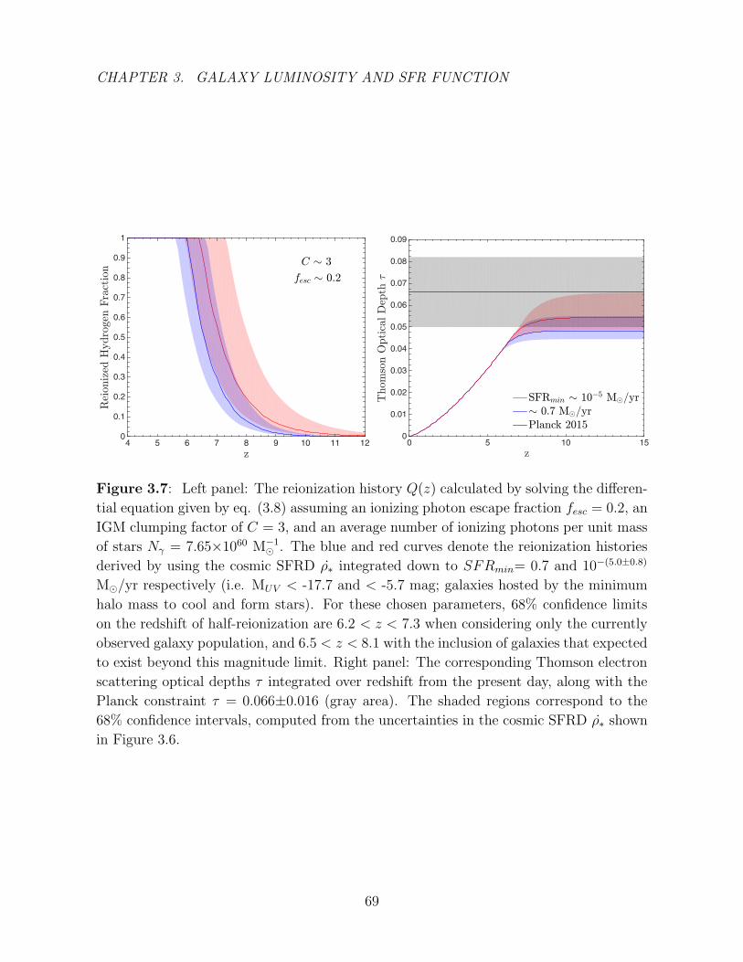
CHAPTER 3. GALAXY LUMINOSITY AND SFR FUNCTION
C 9 3
fesc 9 0.2
z4 5 6 7 8 9 10 11 12
Reion
ized
Hydro
gen
Fra
ctio
n
0
0.1
0.2
0.3
0.4
0.5
0.6
0.7
0.8
0.9
1
z0 5 10 15
Thom
son
Optica
lD
epth=
0
0.01
0.02
0.03
0.04
0.05
0.06
0.07
0.08
0.09
SFRmin 9 10!5 M-/yr9 0.7 M-/yrPlanck 2015
Figure 3.7: Left panel: The reionization history Q(z) calculated by solving the differen-
tial equation given by eq. (3.8) assuming an ionizing photon escape fraction fesc = 0.2, an
IGM clumping factor of C = 3, and an average number of ionizing photons per unit mass
of stars Nγ = 7.65×1060 M−1 . The blue and red curves denote the reionization histories
derived by using the cosmic SFRD ρ∗ integrated down to SFRmin= 0.7 and 10−(5.0±0.8)
M/yr respectively (i.e. MUV < -17.7 and < -5.7 mag; galaxies hosted by the minimum
halo mass to cool and form stars). For these chosen parameters, 68% confidence limits
on the redshift of half-reionization are 6.2 < z < 7.3 when considering only the currently
observed galaxy population, and 6.5 < z < 8.1 with the inclusion of galaxies that expected
to exist beyond this magnitude limit. Right panel: The corresponding Thomson electron
scattering optical depths τ integrated over redshift from the present day, along with the
Planck constraint τ = 0.066±0.016 (gray area). The shaded regions correspond to the
68% confidence intervals, computed from the uncertainties in the cosmic SFRD ρ∗ shown
in Figure 3.6.
69
CHAPTER 3. GALAXY LUMINOSITY AND SFR FUNCTION
the corresponding optical depth (right panel) computed using the cosmic SFRD ρ∗ we
derived from our model UV LFs. We find that the currently observed galaxy population
at magnitudes brighter than MUV ≤ -17.7 (SFR ≥ 0.7 M/yr, blue curve) fully reionize
the universe by redshift z ∼ 6 and that the model corresponding to this magnitude limit
predicts a Thomson optical depth of τ ' 0.048. Integrating further down to MUV ≤ -5.7
(SFR ≥ 10−5 M/yr, red curve) produces a model that reionizes the universe slightly
earlier, at z ∼ 6.5, with a predicted optical depth of τ ' 0.054. The shaded regions
corresponding to each of these curves represent the 68% confidence limits arising solely
from the uncertainties in the normalization of the cosmic SFRD.
Our results for the reionization history are consistent with measurements from
high-redshift quasar and gamma-ray burst spectra, as well as from Lyman alpha emission
in high-z galaxies which collectively indicate that reionization ended near z ' 6 (Bolton
& Haehnelt 2007; Kuhlen & Faucher-Giguere 2012; Chornock et al. 2013; Treu et al.
2013; Schenker et al. 2014; McGreer et al. 2015). Furthermore, the model which includes
the population of low-mass halos with SFRs as faint as 10−5 M/yr produces an optical
depth that is consistent with the previous inferred value by Planck, τ = 0.066 (Planck
Collaboration et al. 2016b), at the 1σ level. These findings, in line with previous analyses,
indicate that a significant population of low-mass star-forming galaxies is necessary for
cosmic reionization and strengthen the conclusion that the bulk of photons responsible
for reionizing the early universe emerged from ultra-faint galaxies.
In order for our model to reproduce the most recent value of τ = 0.078 inferred
from CMB observations by Planck, the average SFR −Mh relation used would have to
allow for larger star formation rates at the low-mass end. One simple way to satisfy such
conditions is to permit SFRav(Mh) to vary according to the average relation derived via
70
CHAPTER 3. GALAXY LUMINOSITY AND SFR FUNCTION
abundance matching for Mh & 1011 M, but decline as a power law for Mh . 1011 M
with a slope of β ∼ 1.3, shallower than the slope derived empirically in section 3.4.1 at
the low mass end. In such a model, the corresponding optical depth would be τ ∼ 0.076,
similar to the latest reduced measurement of τ = 0.078. While the high-redshift LF
functions derived assuming such a form for the average SFR−Mh relation are in tension
with current observations, future measurements taken with JWST will shed more light
on how the LF functions evolve at these low SFRs.
We also note that the results for Q(z) and τ(z) depend on the choices for the escape
fraction fesc, the number of ionizing photons per unit stellar mass Nγ, and the clumping
factor C; if one assumes a smaller clumping factor, or a higher value for fesc or Nγ, the
evolution of Q(z) will be shifted towards higher redshifts and an optical depth closer to
the one measured by Planck Collaboration et al. (2016a) will be obtained. Furthermore,
the ionizing photons of Population III stars are expected to additionally increase the
optical depth at high redshift (Sobral et al. 2015).
3.5 Summary
In this paper, we use the most recent z ∼ 4-8 UV LFs and UV continuum slope
measurements to derive an empirical prediction of the evolution of UV LFs at z > 8.
Assuming a monotonic, one-to-one correspondence between the observed galaxy SFRs
and the host halo masses, we map the shape of the observed z ∼ 4-8 UV LFs to that of
the halo mass function at the respective redshifts. We find that the resulting SFR−Mh
scaling law remains roughly constant over this redshift range and is fairly well fit by a
double power law, SFR ∝Mβh , with β ∼ 0.9 at the high-mass end, i.e. Mh & 2×10¹¹ M,
71

CHAPTER 3. GALAXY LUMINOSITY AND SFR FUNCTION
and β ∼ 1.5 at the low-mass end. We note that the unevolving nature of this relation
with redshift is an empirical result, an explanation for which lies beyond the scope of this
paper. Future work based on semi-analytic models and numerical simulations, as well as
anticipated observations with Atacama Large Millimeter Array (ALMA), are expected
to shed further light on this matter.
Applying this average SFR −Mh relation with an intrinsic scatter of σ ∼ 0.5, we
accurately reproduce the observed SFR functions at 5 . z . 10 (Figures 3.3 and 3.4) and
extend our approach to predict the evolution of the UV LF at redshifts z ∼ 11-20. We
find an evolving characteristic number density φ∗ which decreases as d log φ∗/dz ∼ -0.3, a
gradually steepening faint-end slope, dα/dz ∼ −0.08, and a shifting of the characteristic
luminosity towards fainter values, dM∗UV /dz ∼ 0.4. Given the comoving volume and
magnitude range of an ultra-deep JWST survey, our model predicts that observations
of the LF up to z ∼ 15 are within reach in the absence of gravitational lensing, while
deeper and wider surveys would be necessary to observe higher redshift objects.
We also derive the evolution of the SFR density by integrating the SFRFs down
to various SFR limits, ranging from 0.7 M/yr (corresponding to the faintest object
observed in HUDF12/XDF), to 10−5 M/yr (corresponding to the minimum halo mass
necessary to cool and form stars). The inclusion of galaxies with SFRs well below the
current detection limit results in a more moderately declining cosmic SFRD with redshift
and leads to a fully reionized universe by z ∼ 6.5. Furthermore, the corresponding
predicted optical depth in this model, τ ' 0.054, is consistent with the reduced value
of τ = 0.066±0.016 inferred from CMB observations by Planck at the 1σ level. These
results strengthen the claim that a significant portion of the reionizing photons in the
early universe were emitted by a population of low-mass, star-forming galaxies that have
72
CHAPTER 3. GALAXY LUMINOSITY AND SFR FUNCTION
thus far evaded detection.
3.6 Acknowledgements
We thank R. Smit and R. Bouwens for helpful discussions regarding the SFRF
measurements and for comments on an earlier version of this manuscript. This work
was supported in part by NSF grant AST-1312034. This material is based upon work
supported by the National Science Foundation Graduate Research Fellowship under
Grant No. DGE1144152. Any opinion, findings, and conclusions or recommendations
expressed in this material are those of the authors and do not necessarily reflect the
views of the National Science Foundation.
73
Part II
The Molecular Interstellar Medium
74
Chapter 4
The Ratio of CO to Total Gas Mass
in High-Redshift Galaxies
This thesis chapter originally appeared in the literature as
N. Mashian, A. Sternberg, and A. Loeb, The ratio of CO to
total gas mass in high-redshift galaxies, Monthly Notices of the
Royal Astronomical Society, 435, 2407, 2013
4.1 Abstract
Walter et al. (2012) have recently identified the J=6-5, 5-4, and 2-1 CO rotational
emission lines, and [CII] fine-structure emission line from the star-forming interstellar
medium in the high-redshift submillimeter source HDF 850.1, at z = 5.183. We employ
large velocity gradient (LVG) modeling to analyze the spectra of this source assuming
the [CII] and CO emissions originate from (i) separate virialized regions, (ii) separate
75
CHAPTER 4. CO TO TOTAL GAS MASS IN HIGH-Z GALAXIES
unvirialized regions, (iii) uniformly mixed virialized regions, and (iv) uniformly mixed
unvirialized regions. We present the best fit set of parameters, including for each case the
ratio α between the total hydrogen/helium gas mass and the CO(1-0) line luminosity.
We also present computations of the ratio of H2 mass to [CII] line-luminosity for optically
thin conditions, for a range of gas temperatures and densities, for direct conversion of
[CII] line-luminosities to “ CO-dark” H2 masses. For HDF 850.1 we find that a model in
which the CO and C+ are uniformly mixed in gas that is shielded from UV radiation,
requires a cosmic-ray or X-ray ionization rate of ζ ≈ 3× 10⁻¹⁴ s−1, plausibly consistent
with the large star-formation rate (∼ 103 M yr−1) observed in this source. Enforcing
the cosmological constraint posed by the abundance of dark matter halos in the standard
ΛCDM cosmology and taking into account other possible contributions to the total gas
mass, we find that the two models in which the virialization condition is enforced can
be ruled out at the & 2σ level while the model assuming mixed unvirialized regions is
less likely. We conclude that modeling HDF 850.1’s ISM as a collection of unvirialized
molecular clouds with distinct CO and C+ layers, for which α = 1.2 M (K km s−1
pc2)−1 for the CO to H2 mass-to-luminosity ratio, (similar to the standard ULIRG
value), is most consistent with the ΛCDM cosmology.
4.2 Introduction
Observations of high-redshift CO spectral line emissions have greatly increased our
knowledge of galaxy assembly in the early Universe. At redshifts z∼2, this includes the
discovery of turbulent star-forming disks with cold-gas mass fractions and star-formation
rates significantly larger than in present day galaxies (Daddi et al. 2010; Genzel et al.
76
CHAPTER 4. CO TO TOTAL GAS MASS IN HIGH-Z GALAXIES
2012; Magnelli et al. 2012; Tacconi et al. 2010, 2013). The high star-formation rates
are correlated with large gas masses and luminous CO emission lines (Kennicutt &
Evans 2012) observable to very high redshifts. A prominent example is the luminous
submillimeter and Hubble-Deep-Field source HDF 850.1, which is at a redshift of z =
5.183 as determined by recent detections of CO(6-5), CO(5-4), and CO(2-1) rotational
line emissions, and also [CII] fine-structure emission in this source (Walter et al. 2012).
The high redshift of HDF 850.1 offers the opportunity of setting cosmological constraints
on the conversion factor from CO line luminosities to gas masses, via the implied dark
matter masses and the expected cosmic volume density of halos of a given mass. Such
analysis is the subject of our paper.
CO emitting molecular clouds, which provide the raw material for star formation,
are usually assumed to have undergone complete conversion from atomic to molecular
hydrogen. However, since H2 has strongly forbidden rotational transitions and requires
high temperatures (∼500 K) to excite its rotational lines, it is a poor tracer of cold (.
100 K) molecular gas. Determining H2 gas masses in the interstellar medium (ISM)
of galaxies has therefore relied on tracer molecules. In particular, 12CO is the most
commonly employed tracer of ISM clouds; aside from being the most abundant molecule
after H2, CO has a weak dipole moment (µe = 0.11 Debye) and its rotational levels are
thus excited and thermalized by collisions with H2 at relatively low molecular hydrogen
densities (Solomon & Vanden Bout 2005).
The molecular hydrogen gas mass is often obtained from the CO luminosity by
adopting a mass-to-luminosity conversion factor α = MH2/L′CO(1−0) between the H2
mass and the J =1-0 115 GHz CO rotational transition (Bolatto et al. 2013). The value
for α has been empirically calibrated for the Milky Way Galaxy by three independent
77
CHAPTER 4. CO TO TOTAL GAS MASS IN HIGH-Z GALAXIES
techniques: (i) correlation of optical extinction with CO column densities in interstellar
dark clouds (Dickman 1978); (ii) correlation of gamma-ray flux with the CO line flux in
the Galactic molecular ring (Bloemen et al. 1986; Strong et al. 1988); and (iii) observed
relations between the virial mass and CO line luminosity for Galactic GMCs (Solomon
et al. 1987). These methods have all arrived at the conclusion that the conversion factor
in our Galaxy is fairly constant. The standard Galactic value is α = 4.6 M/(K km−1
pc2). Subsequent studies of CO emission from unvirialized regions in Ultra-Luminous
Infrared Galaxies (ULIRGs) found a significantly smaller ratio. For such systems, α =
0.8 M/(K km−1 pc2) (Downes & Solomon 1998). These values have been adopted by
many (Sanders et al. 1988; Tinney et al. 1990; Wang et al. 1991; Walter et al. 2012)
to convert CO J=1-0 line observations to total molecular gas masses, but without
consideration of the dependence of α on the average molecular gas conditions found in
the sources being considered. Since all current observational studies of α leave its range
and dependence on the average density, temperature, and kinetic state of the molecular
gas still largely unexplored, its applicability to other systems in the local or distant
Universe is less certain (Papadopoulos et al. 2012a).
In this paper, we estimate the CO emitting gas masses in HDF 850.1 using the
large-velocity-gradient (LVG) formalism to fit the observed emission line spectral energy
distribution (SED) for a variety of model configurations, and for a comparison to the
Galactic and ULIRG conversions. In section 4.3 we outline the details of the LVG
approach, including an overview of the escape probability method and a derivation of
the gas mass from the line intensity of the modeled source. In section 4.4, we present the
best fit set of parameters that reproduce HDF 850.1’s detected lines and calculate the
corresponding molecular gas mass, assuming the CO and [CII] emission lines originate
78

CHAPTER 4. CO TO TOTAL GAS MASS IN HIGH-Z GALAXIES
from (i) separate virialized regions, (ii) separate unvirialized regions, (iii)uniformly
mixed virialized regions, and (iv) uniformly mixed unvirialized regions. The inferred
gas masses enable us to set lower-limits on the dark-matter halo mass for HDF 850.1.
In section 4.5 we compare the estimated halo-masses to the number of such objects
expected at high redshift in ΛCDM cosmology, and show that models with lower values
of α are favored. We conclude with a discussion of our findings and their implications in
section 4.6.
4.3 Large Velocity Gradient Model
We start by describing our procedure for quantitatively analyzing the [CII] and CO
emission lines detected at the position of HDF 850.1 using the large velocity gradient
(LVG) approximation. We consider a multi-level system with population densities of the
ith level given by ni. The equations of statistical equilibrium can then be written as :
ni
l∑j 6=i
Rij =l∑j 6=i
njRji (4.1)
where l is the total number of levels included; since the set of l statistical equations is
not independent, one equation may be replaced by the conservation equation
ntot =l∑
j=0
nj (4.2)
where ntot is the number density of the given species in all levels. In our application, ntot
= nCO. Following the notation of Poelman & Spaans (2005), Rij is given in terms of the
Einstein coefficients, Aij and Bij, and the collisional excitation (i < j )and de-excitation
79
CHAPTER 4. CO TO TOTAL GAS MASS IN HIGH-Z GALAXIES
rates (i > j ) Cij:
Rij =
Aij +Bij〈Jij〉+ Cij, (i > j)
Bij〈Jij〉+ Cij, (i < j)
(4.3)
where 〈Jij〉 is the mean radiation intensity corresponding to the transition from level i
to j averaged over the local line profile function φ(νij). The total collisional rates Cij
depend on the individual temperature-dependent rate coefficients and collision partners,
usually H2 and H for CO rotational excitation.
The difficulty in solving this problem is that the mean intensity at any location in
the source is a function of the emission and varying excitation state of the gas all over
the rest of the source, and is thus a nonlocal quantity. To obtain a general solution of
the coupled sets of equations describing radiative transfer and statistical equilibrium,
we adopt the approach developed by Sobolev (1960) and extended by Castor (1970)
and Lucy (1971) and assume the existence of a large velocity gradient in dense clouds.
This assumption is justified given the interstellar molecular line widths which range
from a few up to a few tens of kilometers per second, far in excess of plausible thermal
velocities in the clouds (Goldreich & Kwan 1974). They suggest that these observed
velocity differences arise from large-scale, systematic, velocity gradients across the cloud,
a hypothesis that lies in accord with the constraints provided by observation and theory.
In the limit that the thermal velocity in the cloud is much smaller than the velocity
gradient across the radius of the cloud, the value of 〈Jij〉 at any point in the cloud, when
integrated over the line profile, depends only upon the local value of the source function
and upon the probability that a photon emitted at that point will escape from the cloud
80
CHAPTER 4. CO TO TOTAL GAS MASS IN HIGH-Z GALAXIES
without further interaction. Thus 〈Jij〉 becomes a purely local quantity, given by:
〈Jij〉 = (1− βij)Sij + βijB(νij, TB) (4.4)
where Sij is the line source function,
Sij =2hν3
ij
c2(ginjgjni
− 1)−1 (4.5)
assumed constant through the medium. In this expression gi and gj are the statistical
weights of levels i and j respectively, βij is the “photon escape probability”, and
Bij(νij, TB) is the background radiation with temperature TB. In our models we set TB
to the CMB temperature of 16.9 K at z = 5.183. We ignore contributions from warm
dust (da Cunha et al. 2013).
For a spherical homogenous collapsing cloud, the probability that a photon emitted
in the transition from level i to level j escapes the cloud is given by
βij =1− e−τij
τij(4.6)
where τij is the optical depth in the line,
τij =Aij8π
c3
ν3ij
ntotdv/dr
njgintotgj
(1− gjniginj
). (4.7)
The equations of statistical equilibrium are therefore reduced to the simplified form
l∑j 6=i
(niCij − njCji) + ni
l∑j 6=ij<i
Aijβij −l∑j 6=ij>i
njAjiβji = 0 (4.8)
and can be solved through an iterative process to give the fractional level populations
ni/ntot (for a given choice of densities for the collision partners, usually H2 but also H,
and kinetic temperature Tkin). Assuming the telescope beam contains a large number
of these identical homogeneous collapsing clouds (e.g., Hailey-Dunsheath 2009), the
81
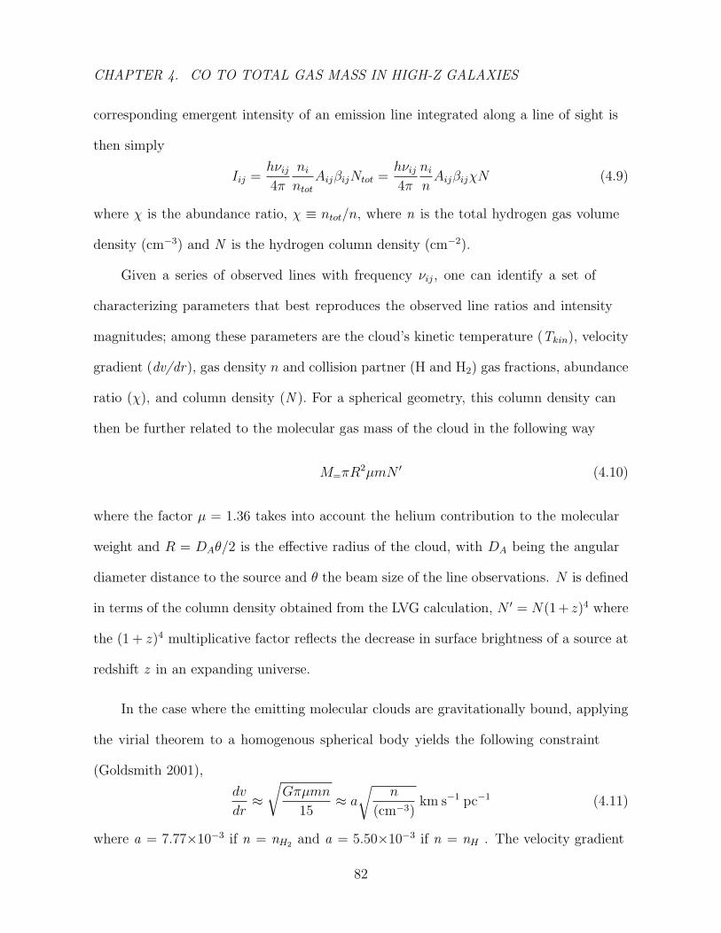
CHAPTER 4. CO TO TOTAL GAS MASS IN HIGH-Z GALAXIES
corresponding emergent intensity of an emission line integrated along a line of sight is
then simply
Iij =hνij4π
nintot
AijβijNtot =hνij4π
ninAijβijχN (4.9)
where χ is the abundance ratio, χ ≡ ntot/n, where n is the total hydrogen gas volume
density (cm−3) and N is the hydrogen column density (cm−2).
Given a series of observed lines with frequency νij, one can identify a set of
characterizing parameters that best reproduces the observed line ratios and intensity
magnitudes; among these parameters are the cloud’s kinetic temperature (Tkin), velocity
gradient (dv/dr), gas density n and collision partner (H and H2) gas fractions, abundance
ratio (χ), and column density (N ). For a spherical geometry, this column density can
then be further related to the molecular gas mass of the cloud in the following way
M=πR2µmN ′ (4.10)
where the factor µ = 1.36 takes into account the helium contribution to the molecular
weight and R = DAθ/2 is the effective radius of the cloud, with DA being the angular
diameter distance to the source and θ the beam size of the line observations. N is defined
in terms of the column density obtained from the LVG calculation, N ′ = N(1 + z)4 where
the (1 + z)4 multiplicative factor reflects the decrease in surface brightness of a source at
redshift z in an expanding universe.
In the case where the emitting molecular clouds are gravitationally bound, applying
the virial theorem to a homogenous spherical body yields the following constraint
(Goldsmith 2001),
dv
dr≈√Gπµmn
15≈ a
√n
(cm−3)km s−1 pc−1 (4.11)
where a = 7.77×10⁻³ if n = nH2 and a = 5.50×10⁻³ if n = nH . The velocity gradient
82

CHAPTER 4. CO TO TOTAL GAS MASS IN HIGH-Z GALAXIES
is inversely proportional to the dynamical time scale. In models where the clouds are
assumed to be virialized, dv/dr and n are no longer independent input parameters of the
model, but rather vary according to eq. (4.11).
For the optically thick 12CO J=1-0 transition line (β ≈ 1/τ), carrying out the LVG
calculations with this additional virialization condition leads to a simple relation between
the gas mass and the CO(1-0) line luminosity,
αCO =MH2
L′CO(1−0)
= 8.6
√nH2/(cm−3)
Texc/(K)M(K km s−1 pc2)−1 (4.12)
where the excitation temperature Texc ≈ Tkin when the emission line is thermalized. (In
this expression we assume complete conversion to H2 so that the gas mass is the H2
mass.) Empirically, the Galactic value of this mass-to-luminosity ratio for virialized
objects bound by gravitational forces is α = MH2/L’CO(1−0) = 4.6 M (K km s−1 pc2)−1
(Solomon & Barrett 1991), corresponding to√nH2/T ∼ 0.5 cm−3/2K−1.
4.4 Analysis of HDF 850.1
4.4.1 Properties of the Galaxy
HDF 850.1, the brightest submillimetre source in the Hubble Deep Field at a wavelength
of 850 micrometers, was discovered by Hughes et al. 1998. A full-frequency scan of
this source by Walter et al. (2012) using the IRAM (Institut de Radioastronomie
Millimetrique) Pleateau de Bure Interferometer and the National Radio Astronomy
Observatory (NRAO) Jansky Very Large Array has detected three CO lines, identified
as the CO(2-1) 230.5 GHz, CO(5-4) 576.4 GHz, and CO(6-5) 691.5 GHz rotational
83

CHAPTER 4. CO TO TOTAL GAS MASS IN HIGH-Z GALAXIES
transitions. [CII] 1900.1 GHz (158 µm), one of the main cooling lines of the star-forming
in stellar medium, has also been detected (Table 4.1). These lines have placed HDF
850.1 in a galaxy over density at z = 5.183, a redshift higher than those of most of the
hundreds of submillimetre-bright galaxies identified thus far.
Walter et al. (2012) used an LVG model to characterize the CO spectral energy
distribution of HDF 850.1 and found that the observed CO line intensities could be fit
with a molecular hydrogen density of 103.2 cm−3, a velocity gradient of 1.2 km s−1pc−1,
and a kinetic temperature of 45 K. Then, assuming α = 0.8 M(K km s−1pc2)−1 as for
ULIRGs, they used the 1-0 line luminosity inferred from their LVG computation to infer
that MH2 = 3.5×10¹⁰ M. However, as Papadopoulos et al. (2012a) argue, adopting
a uniform value of α for ULIRGs neglect its dependence on the density, temperature,
and kinematic state of the gas; this may limit the applicability of computed conversion
factors to other systems in the local or distant Universe.
Here, we broaden the LVG analysis carried out in Walter et al. 2012 and use the
LVG-modeled column density to estimate the total gas mass of the source. We present
several alternative models, each subject to a slightly different constraint. In particular,
Table 4.1. CO and [CII] Line Observations of HDF 850.1
Line νobs Integrated Flux Density Luminosity Intensity
[GHz] [Jy km s−1] [1010 K km s−1 pc2] [erg(s cm2 str)−1]
CO(2-1) 37.286 0.17±0.04 4.1±0.9 (2.16±0.51)×10−9
CO(5-4) 93.202 0.5±0.1 1.9±0.4 (1.59±0.32)×10−8
CO(6-5) 111.835 0.39±0.1 1.0±0.3 (1.49±0.82)×10−8
[CII] 307.383 14.6±0.3 5.0±0.1 (1.5±0.03)×10−6
84
CHAPTER 4. CO TO TOTAL GAS MASS IN HIGH-Z GALAXIES
we first consider the case where the CO and [CII] lines originate from different regions of
the molecular cloud. This picture is consistent with the standard structure of PDRs in
which there is a layer of almost totally ionized carbon at the outer edge, intermediate
regions where the carbon is atomic, and internal regions where the carbon is locked into
CO (Sternberg & Dalgarno 1995; Tielens & Hollenbach 1985; Wolfire et al. 2010). In
this picture then, the hydrogen is fully molecular in the CO emitting regions. We then
consider models in which the CO molecules and C+ ions are uniformly mixed, such that
the line emissions originate in gas at the same temperature and density. These models
resemble conditions found in UV-opaque cosmic-ray dominated dark cores of interstellar
molecular clouds where the chemistry is driven entirely by cosmic-ray ionization. For
HDF850.1, the ionization rates could be significantly higher than in the Milky Way,
leading to enhanced C+ in the UV-shielded regions. In both instances, we perform our
LVG computations assuming (a) virialized clouds for which the virialization condition
(eq. (4.11)) has been imposed and (b) gravitationally-unbound clouds.
To carry out these computations, we use the Mark & Sternberg LVG radiative
transfer code described in Davies et al. (2012). Energy levels, line frequencies and
Einstein A coefficients are taken from the Cologne Database for Molecular Spectroscopy
(CDMS).The excitation and deexcitation rates of the CO rotational levels that are
induced by collisions with H2 are taken from Yang et al. (2010) while the C+ collisional
rate coefficients come from Flower & Launay (1977) and Launay & Roueff (1977).
85
CHAPTER 4. CO TO TOTAL GAS MASS IN HIGH-Z GALAXIES
4.4.2 Separate CO, C+ Virialized Regions
We first consider a model in which the CO and [CII] emission lines detected at the position
of HDF 850.1 originate in separate regions of the molecular gas cloud, regions which are
not necessarily at the same temperature and number density. For self-gravitating clouds
in virial equilibrium, the velocity gradient is no longer an independent input parameter
of the LVG model, but varies with nH2 according to eq. (4.11). To find the unique
solution that yields the two observed line ratios, ICO(6−5)/ICO(2−1) and ICO(6−5)/ICO(5−4),
we assume a canonical value of χCO = 10−4 for the relative CO to H2 abundance and
vary the remaining two parameters, temperature and molecular hydrogen density, over a
large volume of the parameter space. We find, under this virialization constraint, that
the observed CO lines are best fit with a kinetic temperature of 70 K and a molecular
hydrogen number density of 102.6 cm−3 (with a corresponding velocity gradient of ≈ 0.16
km s−1pc−1). The column density that yields the correct line intensity magnitudes is
4.2×1019 cm−2, corresponding to a molecular hydrogen gas mass of MH2 ≈ 2.13×10¹¹
M. The H2 mass to CO luminosity conversion factor obtained in this model is α =
5.1 M(K km s−1 pc2)−1, a value similar to the Galactic conversion factor observed for
virialized molecular clouds in the Milky Way, suggesting that HDF 850.1 may have some
properties in common with our Galaxy.
Reducing the relative CO to H2 abundance by a factor of two, to χCO = 5×10⁻⁵,
results in a best fit solution with a molecular hydrogen gas mass of MH2 ≈ 2.68×10¹¹
M, nearly 25% larger than the value obtained assuming χCO = 10−4. Ranges on the fit
parameter consistent with the observational uncertainties are listed in Tables 4.2 and 4.3.
86
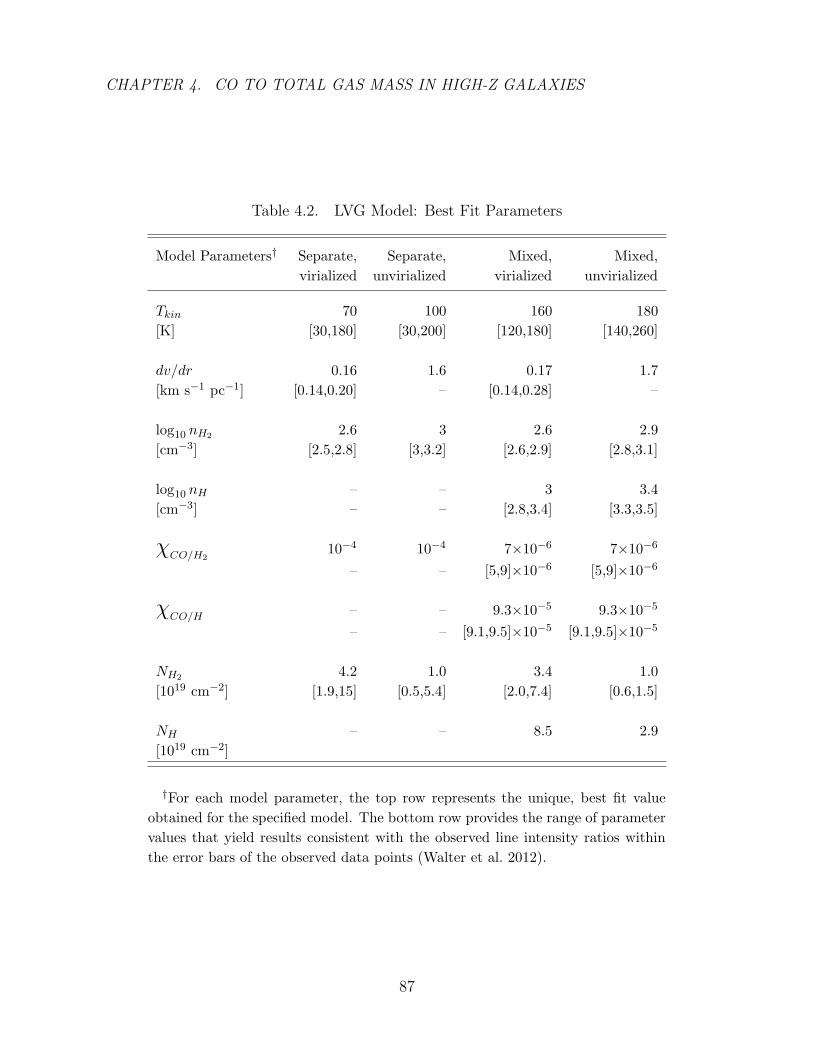
CHAPTER 4. CO TO TOTAL GAS MASS IN HIGH-Z GALAXIES
Table 4.2. LVG Model: Best Fit Parameters
Model Parameters† Separate, Separate, Mixed, Mixed,
virialized unvirialized virialized unvirialized
Tkin 70 100 160 180
[K] [30,180] [30,200] [120,180] [140,260]
dv/dr 0.16 1.6 0.17 1.7
[km s−1 pc−1] [0.14,0.20] – [0.14,0.28] –
log10 nH2 2.6 3 2.6 2.9
[cm−3] [2.5,2.8] [3,3.2] [2.6,2.9] [2.8,3.1]
log10 nH – – 3 3.4
[cm−3] – – [2.8,3.4] [3.3,3.5]
χCO/H210−4 10−4 7×10⁻⁶ 7×10⁻⁶
– – [5,9]×10−6 [5,9]×10−6
χCO/H – – 9.3×10⁻⁵ 9.3×10⁻⁵
– – [9.1,9.5]×10−5 [9.1,9.5]×10−5
NH2 4.2 1.0 3.4 1.0
[1019 cm−2] [1.9,15] [0.5,5.4] [2.0,7.4] [0.6,1.5]
NH – – 8.5 2.9
[1019 cm−2]
†For each model parameter, the top row represents the unique, best fit value
obtained for the specified model. The bottom row provides the range of parameter
values that yield results consistent with the observed line intensity ratios within
the error bars of the observed data points (Walter et al. 2012).
87
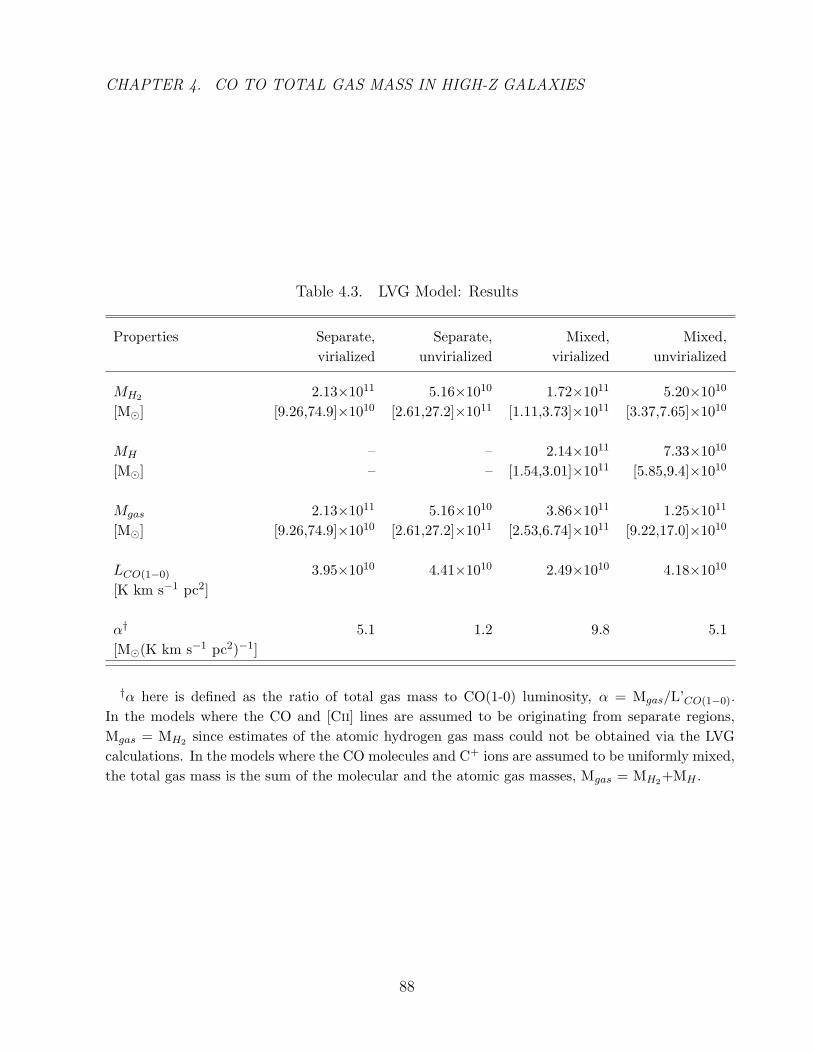
CHAPTER 4. CO TO TOTAL GAS MASS IN HIGH-Z GALAXIES
Table 4.3. LVG Model: Results
Properties Separate, Separate, Mixed, Mixed,
virialized unvirialized virialized unvirialized
MH2 2.13×10¹¹ 5.16×10¹⁰ 1.72×10¹¹ 5.20×10¹⁰
[M] [9.26,74.9]×1010 [2.61,27.2]×1011 [1.11,3.73]×1011 [3.37,7.65]×1010
MH – – 2.14×10¹¹ 7.33×10¹⁰
[M] – – [1.54,3.01]×1011 [5.85,9.4]×1010
Mgas 2.13×10¹¹ 5.16×10¹⁰ 3.86×10¹¹ 1.25×10¹¹
[M] [9.26,74.9]×1010 [2.61,27.2]×1011 [2.53,6.74]×1011 [9.22,17.0]×1010
LCO(1−0) 3.95×10¹⁰ 4.41×10¹⁰ 2.49×10¹⁰ 4.18×10¹⁰
[K km s−1 pc2]
α† 5.1 1.2 9.8 5.1
[M(K km s−1 pc2)−1]
†α here is defined as the ratio of total gas mass to CO(1-0) luminosity, α = Mgas/L’CO(1−0).
In the models where the CO and [CII] lines are assumed to be originating from separate regions,
Mgas = MH2 since estimates of the atomic hydrogen gas mass could not be obtained via the LVG
calculations. In the models where the CO molecules and C+ ions are assumed to be uniformly mixed,
the total gas mass is the sum of the molecular and the atomic gas masses, Mgas = MH2+MH .
88

CHAPTER 4. CO TO TOTAL GAS MASS IN HIGH-Z GALAXIES
4.4.3 Separate CO, C+ Unvirialized Regions
We then consider a model in which the CO and [CII] emission lines are assumed to
originate from separate regions of gravitationally-unbound molecular clouds. Since
unvirialized clouds generally demonstrate a higher degree of turbulence relative to their
virialized counterparts, we expect the velocity gradient in this model to be greater
than the velocity gradient obtained for the virialized model, (dv/dr)virialized ≈ 0.16 km
s−1pc−1. We therefore fix the velocity gradient to be ten times the virialized value,
(dv/dr)unvirialized = 1.6 km s−1pc−1, and, assuming a canonical value of χCO = 10−4,
find the solution that yields the two observed line ratios by varying T and nH2 . We
find, under these assumptions, that the CO SED is best fit with a molecular hydrogen
density of 103 cm−3 and a kinetic temperature of 100 K. For this set of parameters,
the beam-averaged H2 column density is NH2 ≈ 1.0×1019 cm−2, giving an associated
molecular gas mass of MH2 ≈ 5.16×10¹⁰ M. This estimate of the gas mass is nearly
50% larger than that obtained by Walter et al. (2012) by applying the H2 mass-to-CO
luminosity relation with the typically adopted conversion factor for ULIRGs, α = 0.8 M
(K km s−1 pc2)−1. Given our inferred H2 gas mass and predicted CO(1-0) line luminosity
from our LVG fit, we find that α = 1.2 M (K km s−1 pc2)−1, in this model.
The increase in molecular hydrogen density and the reduction in inferred mass
(relative to the values obtained in the previous model where the virialization condition
was imposed) arise from our assumption that the velocity gradient in this model is greater
than the velocity gradient obtained in the virialized case. For a fixed χ, the optical
depth drops with increasing dv/dr (eq. (4.7)); since β, the probability of an emitted
photon escaping, correspondingly increases, the radiation is less “trapped” and a higher
89
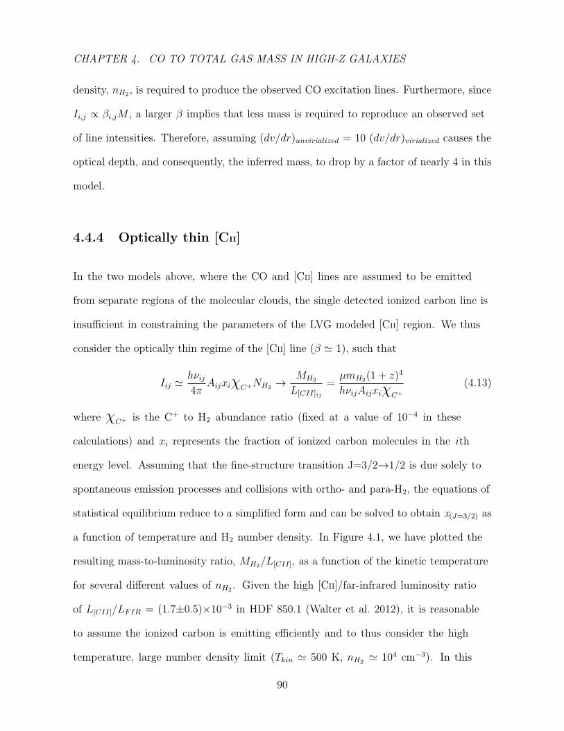
CHAPTER 4. CO TO TOTAL GAS MASS IN HIGH-Z GALAXIES
density, nH2 , is required to produce the observed CO excitation lines. Furthermore, since
Ii,j ∝ βi,jM , a larger β implies that less mass is required to reproduce an observed set
of line intensities. Therefore, assuming (dv/dr)unvirialized = 10 (dv/dr)virialized causes the
optical depth, and consequently, the inferred mass, to drop by a factor of nearly 4 in this
model.
4.4.4 Optically thin [CII]
In the two models above, where the CO and [CII] lines are assumed to be emitted
from separate regions of the molecular clouds, the single detected ionized carbon line is
insufficient in constraining the parameters of the LVG modeled [CII] region. We thus
consider the optically thin regime of the [CII] line (β ' 1), such that
Iij 'hνij4π
AijxiχC+NH2 →MH2
L[CII]ij
=µmH2(1 + z)4
hνijAijxiχC+
(4.13)
where χC+ is the C+ to H2 abundance ratio (fixed at a value of 10−4 in these
calculations) and xi represents the fraction of ionized carbon molecules in the ith
energy level. Assuming that the fine-structure transition J=3/2→1/2 is due solely to
spontaneous emission processes and collisions with ortho- and para-H2, the equations of
statistical equilibrium reduce to a simplified form and can be solved to obtain x(J=3/2) as
a function of temperature and H2 number density. In Figure 4.1, we have plotted the
resulting mass-to-luminosity ratio, MH2/L[CII], as a function of the kinetic temperature
for several different values of nH2 . Given the high [CII]/far-infrared luminosity ratio
of L[CII]/LFIR = (1.7±0.5)×10−3 in HDF 850.1 (Walter et al. 2012), it is reasonable
to assume the ionized carbon is emitting efficiently and to thus consider the high
temperature, large number density limit (Tkin ' 500 K, nH2 ' 104 cm−3). In this
90
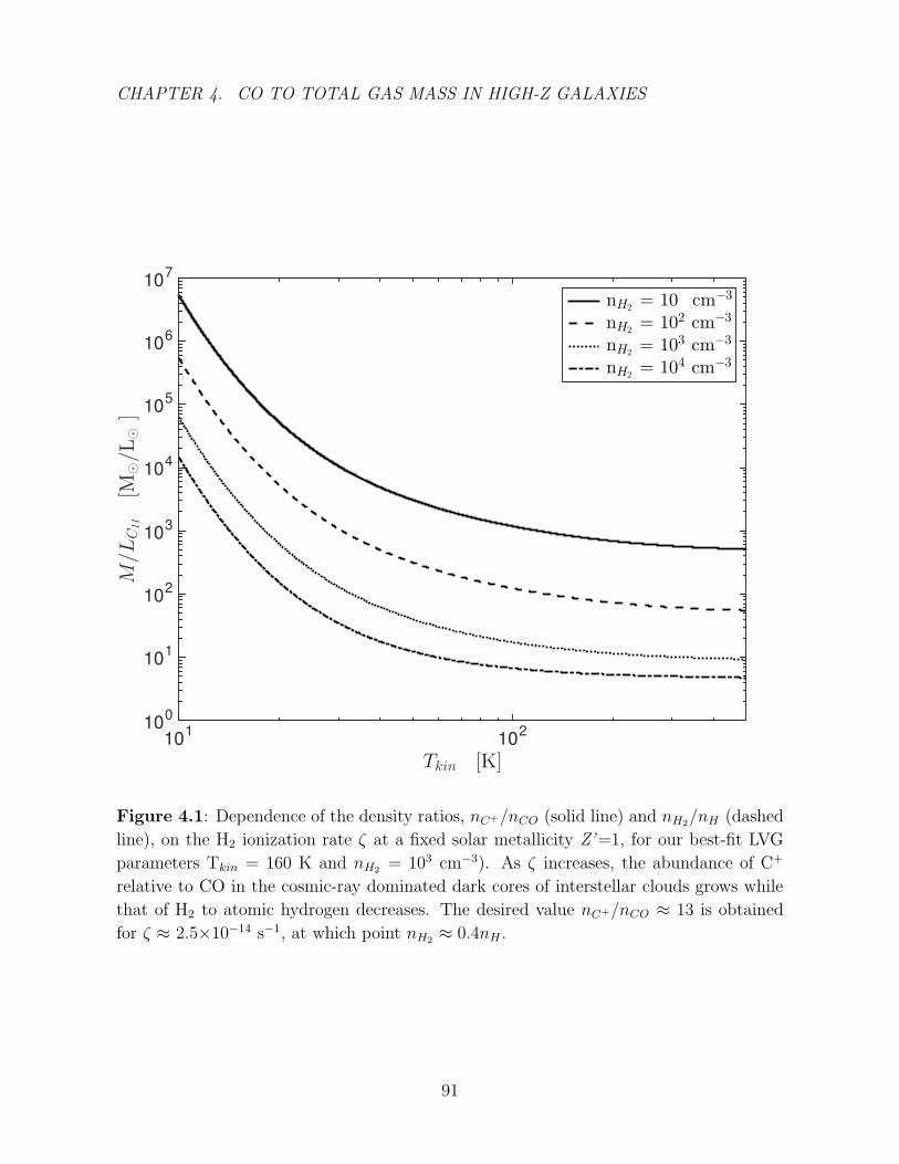
CHAPTER 4. CO TO TOTAL GAS MASS IN HIGH-Z GALAXIES
Tkin [K]10
110
2
M/LC
II
[M⊙/L
⊙]
100
101
102
103
104
105
106
107
nH2= 10 cm−3
nH2= 102 cm−3
nH2= 103 cm−3
nH2= 104 cm−3
Figure 4.1: Dependence of the density ratios, nC+/nCO (solid line) and nH2/nH (dashed
line), on the H2 ionization rate ζ at a fixed solar metallicity Z’=1, for our best-fit LVG
parameters Tkin = 160 K and nH2 = 103 cm−3). As ζ increases, the abundance of C+
relative to CO in the cosmic-ray dominated dark cores of interstellar clouds grows while
that of H2 to atomic hydrogen decreases. The desired value nC+/nCO ≈ 13 is obtained
for ζ ≈ 2.5×10⁻¹⁴ s−1, at which point nH2 ≈ 0.4nH .
91
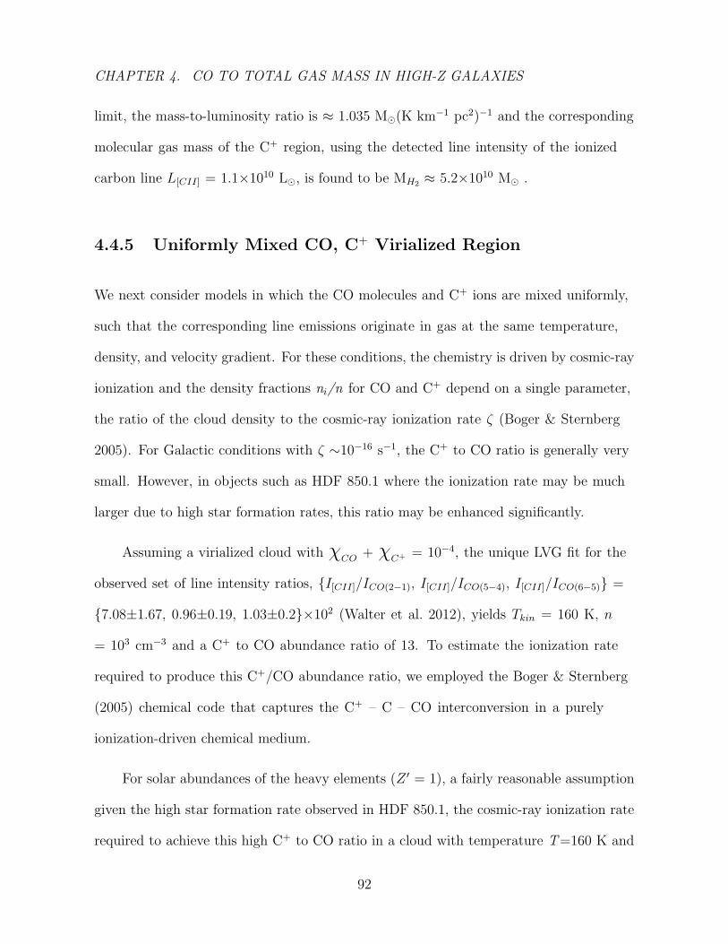
CHAPTER 4. CO TO TOTAL GAS MASS IN HIGH-Z GALAXIES
limit, the mass-to-luminosity ratio is ≈ 1.035 M(K km−1 pc2)−1 and the corresponding
molecular gas mass of the C+ region, using the detected line intensity of the ionized
carbon line L[CII] = 1.1×10¹⁰ L, is found to be MH2 ≈ 5.2×10¹⁰ M .
4.4.5 Uniformly Mixed CO, C+ Virialized Region
We next consider models in which the CO molecules and C+ ions are mixed uniformly,
such that the corresponding line emissions originate in gas at the same temperature,
density, and velocity gradient. For these conditions, the chemistry is driven by cosmic-ray
ionization and the density fractions ni/n for CO and C+ depend on a single parameter,
the ratio of the cloud density to the cosmic-ray ionization rate ζ (Boger & Sternberg
2005). For Galactic conditions with ζ ∼10−16 s−1, the C+ to CO ratio is generally very
small. However, in objects such as HDF 850.1 where the ionization rate may be much
larger due to high star formation rates, this ratio may be enhanced significantly.
Assuming a virialized cloud with χCO + χC+ = 10−4, the unique LVG fit for the
observed set of line intensity ratios, I[CII]/ICO(2−1), I[CII]/ICO(5−4), I[CII]/ICO(6−5) =
7.08±1.67, 0.96±0.19, 1.03±0.2×10² (Walter et al. 2012), yields Tkin = 160 K, n
= 103 cm−3 and a C+ to CO abundance ratio of 13. To estimate the ionization rate
required to produce this C+/CO abundance ratio, we employed the Boger & Sternberg
(2005) chemical code that captures the C+ – C – CO interconversion in a purely
ionization-driven chemical medium.
For solar abundances of the heavy elements (Z ′ = 1), a fairly reasonable assumption
given the high star formation rate observed in HDF 850.1, the cosmic-ray ionization rate
required to achieve this high C+ to CO ratio in a cloud with temperature T=160 K and
92
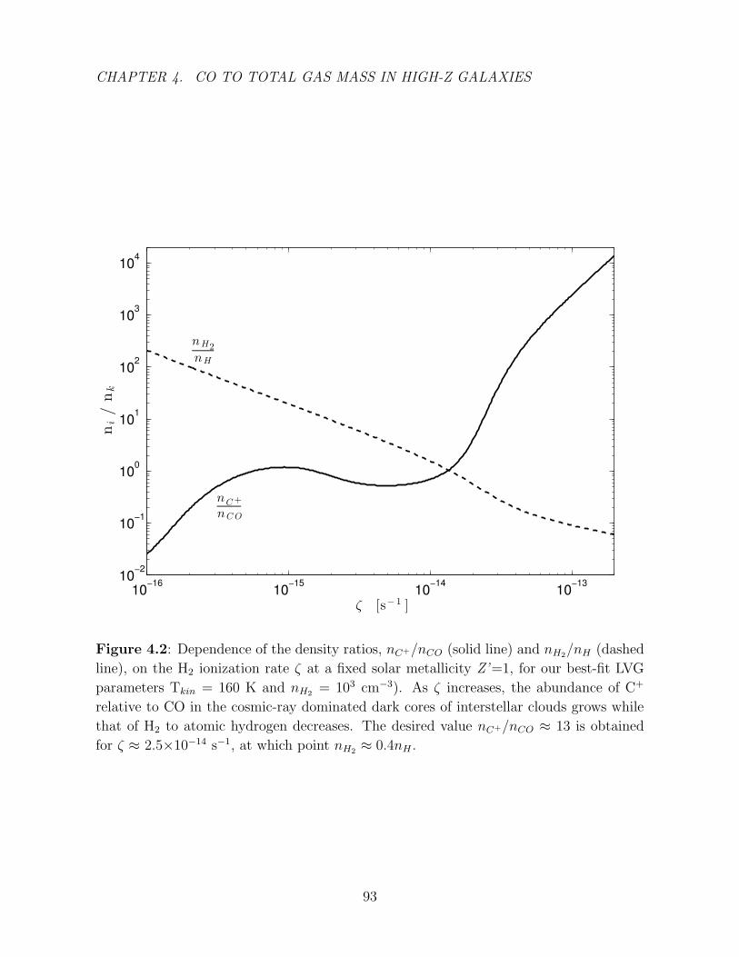
CHAPTER 4. CO TO TOTAL GAS MASS IN HIGH-Z GALAXIES
10−16
10−15
10−14
10−13
10−2
10−1
100
101
102
103
104
ζ [s− 1 ]
ni/nk
nH2
nH
nC+
nCO
Figure 4.2: Dependence of the density ratios, nC+/nCO (solid line) and nH2/nH (dashed
line), on the H2 ionization rate ζ at a fixed solar metallicity Z’=1, for our best-fit LVG
parameters Tkin = 160 K and nH2 = 103 cm−3). As ζ increases, the abundance of C+
relative to CO in the cosmic-ray dominated dark cores of interstellar clouds grows while
that of H2 to atomic hydrogen decreases. The desired value nC+/nCO ≈ 13 is obtained
for ζ ≈ 2.5×10⁻¹⁴ s−1, at which point nH2 ≈ 0.4nH .
93

CHAPTER 4. CO TO TOTAL GAS MASS IN HIGH-Z GALAXIES
density nH2=103 cm−3 is of order ζ ' 2.5×10⁻¹⁴ s−1 (Figure 4.2). This is significantly
enhanced compared to the Milky Way value, ζ ∼10−16 s−1, and is plausibly consistent
with the fact that HDF 850.1 has a star-formation rate of 850 solar masses per year, a
value which is larger than the measured Galactic SFR by a factor of 103 (Walter et al.
2012).
Furthermore, for such a high cosmic-ray ionization rate of this magnitude, the
hydrogen is primarily atomic for the implied LVG gas density. We find that the ratio
of molecular hydrogen to atomic hydrogen in the interstellar clouds is nH2/nH ≈ 0.4
(Figure 4.2). We thus replace H2 with H as the dominant collision partner. Given the
uncertain CO-H rotational excitation rates (see Shepler et al. 2007), we assume that the
rate coefficients are equal to the rates for collisions with ortho-H2 (Flower & Pineau Des
Forets 2010). We find that the observed CO and [CII] lines together are best fit with a
temperature of 160 K, an atomic hydrogen number density of nH = 103 cm−3 (with a
corresponding velocity gradient of 0.17 km s−1 pc−1), and an abundance ratio (relative
to H) of 9.3×10⁻⁵ and 7×10⁻⁶ for C+ and CO respectively. The column density that
yields the correct line intensity magnitudes is 8.5×1019 cm−2, corresponding to an atomic
hydrogen gas mass of MH ≈ 2.14×10¹¹ M. The molecular hydrogen mass is then MH2
= 2(nH2/nH)MH ≈ 1.72×10¹¹ M and the total gas mass estimate is Mgas ≈ 3.86×10¹¹
M. The corresponding conversion factor in this model is α = 9.8 M(K km s−1 pc2)−1,
where α is now defined as the total gas mass to CO luminosity ratio.
Reducing the fixed sum of abundance ratios (relative to H) of CO and C+ by a
factor of two, to χCO + χC+ = 5×10⁻⁵, results in a best fit solution with a total gas
mass of Mgas ≈ 4.57×10¹¹ M, nearly 20% larger than the value obtained assuming χCO
+ χC+ = 10−4.
94
CHAPTER 4. CO TO TOTAL GAS MASS IN HIGH-Z GALAXIES
4.4.6 Uniformly Mixed CO, C+ Unvirialized Region
In the case where we assume gravitationally-unbound molecular clouds, we again find
a best fit model with a C+ to CO ratio of χC+/χCO ≈ 13, indicating that atomic
hydrogen is the dominant collision partner in the LVG calculations. We thus calculate
a three-dimensional grid of model CO and [CII] lines, varying Tkin, nH , and the relative
abundances χ[CII] and χCO, with the constraints that χCO + χC+ = 10−4 and
(dv/dr)unvirialized = 10(dv/dr)virialized = 1.7 km s−1 pc−1 . The observed set of CO
and [CII] lines, assumed to have been emitted from the same region, are fit best with
a temperature of 180 K, an atomic hydrogen number density of 103.4 cm−3 and an
abundance ratio of 9.3×10⁻⁵ and 7×10⁻⁶ for C+ and CO respectively. For this set
of parameters, the beam-averaged H column density is well constrained to be NH ≈
2.9×1019 cm−2. This corresponds to an atomic and molecular gas mass of MH ≈
7.33×10¹⁰ M and MH2 ≈ 5.20× 10¹⁰ M respectively, yielding a total gas mass estimate
of Mgas ≈ 1.25×10¹¹ M. The ratio of the total gas mass to the CO luminosity in this
model is α = 5.1 M(K km s−1 pc2)−1.
4.5 Cosmological Constraints
Our inferred gas masses enable us to set cosmological constraints. For a particular set
of cosmological parameters, the number density of dark matter halos of a given mass
can be inferred from the halo mass function. The Sheth-Tormen mass function, which is
based on an ellipsoidal collapse model, expresses the comoving number density of halos
95
CHAPTER 4. CO TO TOTAL GAS MASS IN HIGH-Z GALAXIES
n per logarithm of halo mass M as,
nST (M) =dn
dlogM= A
√2a
π
ρmM
dν
dlogM(1 +
1
(aν2)p)e−aν
2/2 (4.14)
where a reasonably good fit to simulations can be obtained by setting A = 0.322, a
= 0.707, and p = 0.3 (Sheth & Tormen 1999). Here, ρm is the mean mass density of
the universe and ν = δcrit(z)/σ(M) is the number of standard deviations away from
zero that the critical collapse overdensity represents on mass scale M. Integrating this
comoving number density over a halo mass range and volume element thus yields N, the
expectation value of the total number of halos observed within solid angle A with mass
greater than some Mh and redshift larger than some z,
N(z,Mh) =c
H0
A
∫ ∞z
dzDA(z)2√
Ωm(1 + z)3 + ΩΛ
∫ ∞Mh
dlogMdn
dlogM(4.15)
where H0 is the Hubble constant, DA is the angular diameter distance, and Ωm and ΩΛ
are the present-day density parameters of matter and vacuum, respectively.
Under the assumption that the number of galaxies in the field of observation follows
a Poisson distribution, the probability of observing at least one such object in the field is
then P = 1−F (0, N) where F (0, N) is the Poisson cumulative distribution function with
a mean of N . Given the detection of HDF 850.1, we can say that out of the hundreds
of submillimetre-bright galaxies identified so far, at least one has been detected in the
Hubble Deep Field at a redshift z > 5 with a halo mass greater than or equal to the halo
mass associated with this source. This observation, taken together with the theoretical
number density predicted by the Sheth-Tormen mass function, implies that an atomic
model that yields an expectation value N can be ruled out at a confidence level of
F (0, N(5,Mh,min)) (4.16)
96
CHAPTER 4. CO TO TOTAL GAS MASS IN HIGH-Z GALAXIES
where the solid angle covered by the original SCUBA field in which HDF850.1 was
discovered is ' 9 arcmin2 (Hughes et al. 1998) and a ΛCDM cosmology is assumed with
H0 = 70 km s−1 Mpc−1, ΩΛ = 0.73, and Ωm = 0.27 (Komatsu et al. 2011). Mh,min,
the minimum inferred halo mass for HDF 850.1, is related to the halo’s minimum
baryonic mass component, a quantity derived in section 4.4 via the LVG technique, in
the following way,
Mh,min =Ωm
Ωb
Mb,min (4.17)
where the baryonic and the total matter density parameters are Ωb = 0.05 and Ωm =
0.27 respectively. Each model’s estimate of the minimum baryonic mass associated with
HDF 850.1 therefore corresponds to an estimate of N(5,Mh,min) and respectively yields
the certainty with which the model can be discarded.
The confidence with which models can be ruled out on this basis is plotted as a
function of the minimum baryonic mass estimated by the model (solid curve in Figure
4.3). To check the consistency of the four LVG models considered in section 4.4 with
these results, dashed lines representing the masses derived from each model are included
in the plot (upper left panel). Assuming the CO and [CII] molecules are uniformly mixed
in virialized clouds results in a baryonic mass Mb,min = 3.86×10¹¹ M. The probability
of observing at least one such source, with a corresponding halo mass Mh ≥ 2.1×10¹²
M, is ∼ 7×10⁻²; this model can thus be ruled out at the 1.8σ level (solid). The model
which postulate separate virialized regions (dashed) can be ruled out with relatively less
certainty, at the 1σ level. On the other hand, modeling the CO and [CII] emission lines
as originating from mixed (dotted) or separate (dash-dot) unvirialized regions, results in
minimum baryonic masses which are consistent with the constraint posed by eq. (4.15).
We expect to find N ∼ 1.5 and 10 such halos, respectively, at a redshift z ≥ 5. The
97
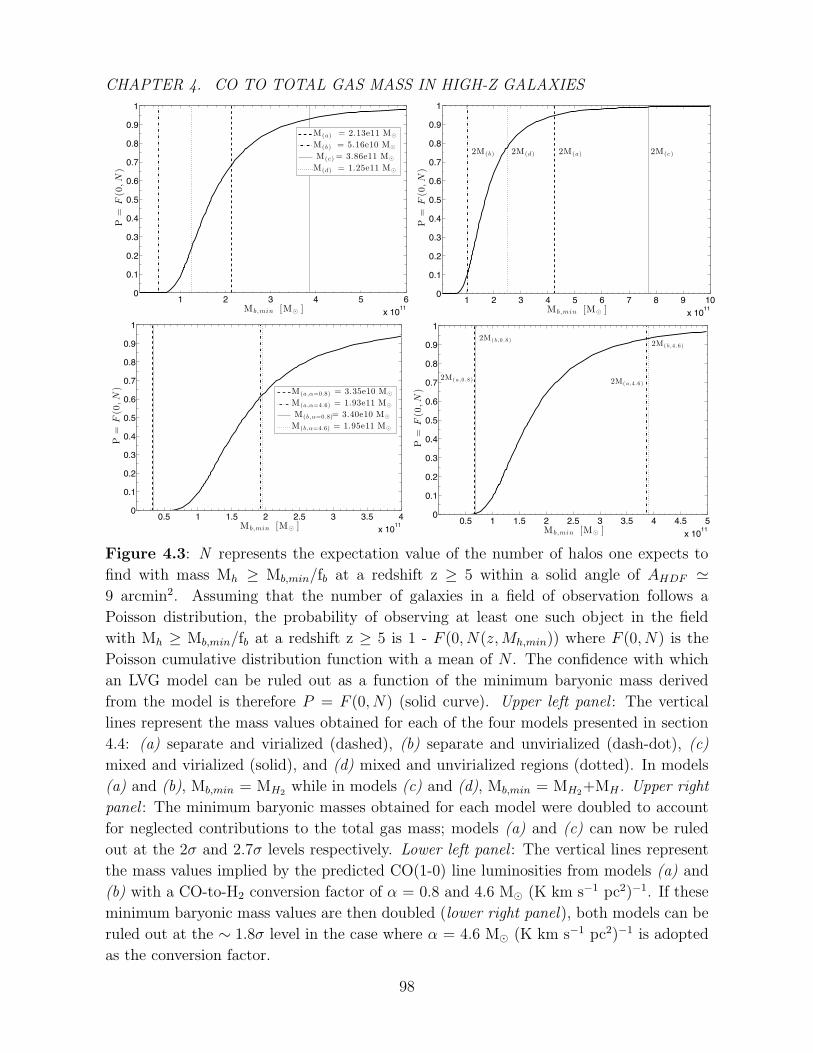
CHAPTER 4. CO TO TOTAL GAS MASS IN HIGH-Z GALAXIES
1 2 3 4 5 6x 10¹¹
0
0.1
0.2
0.3
0.4
0.5
0.6
0.7
0.8
0.9
1
Mb,min [M⊙ ]
P=
F(0,N
)
M(a) = 2.13e11 M⊙
M(b ) = 5.16e10 M⊙
M(c ) = 3.86e11 M⊙
M(d ) = 1.25e11 M⊙
1 2 3 4 5 6 7 8 9 10x 1011
0
0.1
0.2
0.3
0.4
0.5
0.6
0.7
0.8
0.9
1
Mb,min [M⊙ ]
P=
F(0,N
)
2M(a)2M(b ) 2M(c )2M(d )
0.5 1 1.5 2 2.5 3 3.5 4x 10¹¹
0
0.1
0.2
0.3
0.4
0.5
0.6
0.7
0.8
0.9
1
Mb,min [M⊙ ]
P=
F(0,N
) M(a,α=0.8) = 3.35e10 M⊙
M(a,α=4.6) = 1.93e11 M⊙
M(b ,α=0.8)= 3.40e10 M⊙
M(b ,α=4.6) = 1.95e11 M⊙
0.5 1 1.5 2 2.5 3 3.5 4 4.5 5x 10¹¹
0
0.1
0.2
0.3
0.4
0.5
0.6
0.7
0.8
0.9
1
Mb,min [M⊙ ]
P=
F(0,N
)
2M( a,0 .8)
2M( b ,0 .8)
2M( a,4 .6)
2M( b ,4 .6)
Figure 4.3: N represents the expectation value of the number of halos one expects to
find with mass Mh ≥ Mb,min/fb at a redshift z ≥ 5 within a solid angle of AHDF '9 arcmin2. Assuming that the number of galaxies in a field of observation follows a
Poisson distribution, the probability of observing at least one such object in the field
with Mh ≥ Mb,min/fb at a redshift z ≥ 5 is 1 - F (0, N(z,Mh,min)) where F (0, N) is the
Poisson cumulative distribution function with a mean of N . The confidence with which
an LVG model can be ruled out as a function of the minimum baryonic mass derived
from the model is therefore P = F (0, N) (solid curve). Upper left panel : The vertical
lines represent the mass values obtained for each of the four models presented in section
4.4: (a) separate and virialized (dashed), (b) separate and unvirialized (dash-dot), (c)
mixed and virialized (solid), and (d) mixed and unvirialized regions (dotted). In models
(a) and (b), Mb,min = MH2 while in models (c) and (d), Mb,min = MH2+MH . Upper right
panel : The minimum baryonic masses obtained for each model were doubled to account
for neglected contributions to the total gas mass; models (a) and (c) can now be ruled
out at the 2σ and 2.7σ levels respectively. Lower left panel : The vertical lines represent
the mass values implied by the predicted CO(1-0) line luminosities from models (a) and
(b) with a CO-to-H2 conversion factor of α = 0.8 and 4.6 M (K km s−1 pc2)−1. If these
minimum baryonic mass values are then doubled (lower right panel), both models can be
ruled out at the ∼ 1.8σ level in the case where α = 4.6 M (K km s−1 pc2)−1 is adopted
as the conversion factor.
98

CHAPTER 4. CO TO TOTAL GAS MASS IN HIGH-Z GALAXIES
fact that the expected average number of observed sources for the latter model is much
higher than the actual number of sources observed may be due to the incompleteness of
the conducted survey and is therefore not grounds for ruling out this model.
The baryonic masses, obtained via the LVG method, represent conservative
estimates of the total baryonic content associated with HDF 850.1. In particular, mass
contributions from any ionized gas or stars residing in the galaxy are not taken into
account, and in the models where a layered cloud structure is assumed, the atomic
hydrogen mass component is left undetermined. Furthermore, ejection of baryons to
the IGM through winds may result in a halo baryon mass fraction that is smaller than
the cosmic ratio, Ωb/Ωm, used in this paper, resulting in a conservative estimate of
the minimum halo mass. We therefore consider the effects on the predicted number
of observed halos, N(Mh,min), if the minimum baryonic mass derived for each model is
doubled, e.g. assuming a molecular-gas mass fraction of ∼ 1/2 (Tacconi et al. 2013).
Using these more accurate estimates of HDF 850.1’s baryonic mass, we find that the two
models in which the virialization condition is enforced can be ruled out at the ∼ 2.7σ
and 2σ level for the mixed and separate models, respectively (upper right panel).
For comparison, we also consider the gas masses implied by the CO(1-0) line
luminosities predicted by the two models where distinct CO and C+ layers are assumed
(lower left panel). Adopting a CO-to-H2 conversion factor of α = 0.8 (K km s−1 pc2)−1,
we find that enforcing the cosmological constraint posed by the abundance of dark
matter halos does not rule out either of the two models in which separate CO and C+
regions were assumed, even if the minimum baryonic masses are doubled to account for
neglected contributions to the total gas mass (lower right panel). If a conversion factor
of α = 4.6 (K km s−1 pc2)−1 is used, both models can be ruled out at the ∼ 1σ level and
99
CHAPTER 4. CO TO TOTAL GAS MASS IN HIGH-Z GALAXIES
increasing these obtained masses by a factor of two drives up the sigma levels to ∼ 1.8σ
for both models.
4.6 Summary
In this paper, we employed the LVG method to explore alternate model configurations
for the CO and C+ emission lines regions in the high-redshift source HDF 850.1. In
particular, we considered emissions originating from (i) separate virialized regions,
(ii) separate unvirialized regions, (iii) uniformly mixed virialized regions, and (iv)
uniformly mixed unvirialized regions. For models (i) and (ii) where separate CO and
C+ regions were assumed, the kinetic temperature, Tkin, and the molecular hydrogen
density, nH2 , were fit to reproduce the two observed line ratios, ICO(6−5)/ICO(2−1) and
ICO(6−5)/ICO(5−4), for a fixed canonical value of the CO abundance (relative to H2),
χCO = 10−4. The column density of molecular hydrogen, NH2 , was then fit to yield
the correct line intensity magnitudes and the molecular gas mass was derived for each
respective model. In models (iii) and (iv) where the CO molecules and C+ ions were
assumed to be uniformly mixed with abundance ratios that satisfied the constraint, χCO
+ χC+ = 10−4, we found that a relatively high ionization rate of ζ ' 2.5×10⁻¹⁴ s−1 is
necessary to reproduce the set of observed line ratios, I[CII]/ICO(2−1), I[CII]/ICO(5−4),
I[CII]/ICO(6−5). Since the hydrogen in a cloud experiencing an ionization rate of this
magnitude is primarily atomic, two additional parameters, nH and NH , were introduced
and the set of LVG parameters, Tkin, nH2, nH , χCO, χC+, NH2 , NH, were fit and used
to obtain both a molecular and an atomic hydrogen gas mass for each model. The gas
masses derived by employing the LVG technique thus represent conservative estimates of
100
CHAPTER 4. CO TO TOTAL GAS MASS IN HIGH-Z GALAXIES
the minimum baryonic mass associated with HDF 850.1.
These estimates were then used, together with the Sheth-Tormen mass function
for dark matter halos to calculate the average number of halos with mass Mh ≥ Mb,min
that each model predicts to find within the HDF survey volume. Given that at least
one such source has been detected, we found that models (i) and (iii) can be ruled
out at the 1σ and 1.8σ levels respectively. The confidence with which these models
are ruled out increases if a less conservative estimate of the baryonic mass is taken;
increasing the LVG-modeled gas masses by a factor of two to account for neglected
contributions to the total baryonic mass, drives up these sigma levels to ∼ 2σ and 2.7σ
respectively. Furthermore, model (iv) can now be ruled out at the 1σ level as well. We
are therefore led to the conclusion that HDF 850.1 is modeled best by a collection of
unvirialized molecular clouds with distinct CO and C+ layers, as in PDR models. The
LVG calculations for this model yield a kinetic temperature of 100 K, a velocity gradient
of 1.6 km s−1 pc−1, a molecular hydrogen density of 103 cm−3, and a column density of
1019 cm−2. The corresponding molecular gas mass obtained using this LVG approach is
MH2 ≈ 5.16×10¹⁰ M. For this preferred model we find that the CO-to-H2 luminosity to
mass ratio is α = 1.2 (K km s−1 pc2)−1, close to the value found for ULIRGs in the local
universe.
4.7 Acknowledgements
We thank Dean Mark for his assistance with the LVG computations. This work was
supported by the Raymond and Beverly Sackler Tel Aviv University-Harvard/ITC
Astronomy Program. A.L. acknowledges support from the Sackler Professorship by
101

CHAPTER 4. CO TO TOTAL GAS MASS IN HIGH-Z GALAXIES
Special Appointment at Tel Aviv University. This work was also supported in part by
NSF grant AST-0907890 and NASA grants NNX08AL496 andNNA09DB30A (for A.L.).
102

Chapter 5
High-J CO Sleds in Nearby Infrared
Bright Galaxies Observed by
Herschel/PACS
This thesis chapter originally appeared in the literature as
N. Mashian, E. Sturm, A. Sternberg, A. Janssen, S. Hailey-
Dunsheath, J. Fischer, A. Contursi, E. Gonzalez-Alfonso, J.
Gracia-Carpio, A. Poglitsch, S. Veilleux, R. Davies, R. Genzel,
D. Lutz, L. Tacconi, A. Verma, A. Weiß, E. Polisensky, and T.
Nikola, High-J CO SLEDs in nearby infrared bright galaxies
observed by Herschel/PACS, The Astrophysical Journal, 802,
81, 2015
103
CHAPTER 5. HIGH-J CO IN NEARBY GALAXIES
5.1 Abstract
We report the detection of far-infrared (FIR) CO rotational emission from nearby active
galactic nuclei (AGN) and starburst galaxies, as well as several merging systems and
Ultra-Luminous Infrared Galaxies (ULIRGs). Using Herschel-PACS, we have detected
transitions in the Jupp = 14 - 20 range (λ ∼ 130 - 185 µm, ν ∼ 1612 - 2300 GHz)
with upper limits on (and in two cases, detections of) CO line fluxes up to Jupp = 30.
The PACS CO data obtained here provide the first well-sampled FIR extragalactic CO
Spectral Line Energy Distributions (SLEDs) for this range, and will be an essential
reference for future high redshift studies. We find a large variety in overall SLED
shape, demonstrating the uncertainties in relying solely on high-J CO diagnostics to
characterize the excitation source of a galaxy. Combining our data with low-J line
intensities taken from the literature, we present a CO ratio-ratio diagram and discuss
its potential diagnostic value in distinguishing excitation sources and physical properties
of the molecular gas. We find that the position of a galaxy on such a diagram is less
a signature of its excitation mechanism, but rather an indicator of the presence (or
absence) of warm, dense molecular gas. We then quantitatively analyze the CO emission
from a subset of the detected sources with Large Velocity Gradient (LVG) radiative
transfer models to fit the CO SLEDs. Using both single-component and two-component
LVG models to fit the kinetic temperature, velocity gradient, number density and column
density of the gas, we derive the molecular gas mass and the corresponding CO-to-H2
conversion factor, αCO, for each respective source. For the ULIRGs we find α values
in the canonical range 0.4 - 5 M/(K km−1pc−2, while for the other objects, α varies
between 0.2 and 14. Finally, we compare our best-fit LVG model results with those
104
CHAPTER 5. HIGH-J CO IN NEARBY GALAXIES
obtained in previous studies of the same galaxies and comment on any differences.
5.2 Introduction
Molecular spectral line energy distributions (SLEDs) provide us with the opportunity
to probe the average state of the molecular gas in galaxies and estimate the total and
star-forming molecular gas masses in these sources. Carbon monoxide (CO), the most
abundant molecule after molecular hydrogen, is the most commonly employed tracer of
interstellar molecular gas. With the small gaps between its energy levels allowing for a
fine sampling of density-temperature relations, CO has become an important tool in the
study of the star formation energetics and the effects of AGN in nearby galaxies.
The lowest 3 rotational transitions of CO, which trace the cooler gas component,
are relatively easily accessible with ground-based radio and submillimeter telescopes,
and have been observed in many local galaxies. On the other hand, far-IR CO rotational
lines, with Jupp ≥ 13, arise from states 500 - 7000 K above ground and have critical
densities of 106 ∼ 108 cm−3 (Hailey-Dunsheath et al. 2012). These lines, which trace the
warmer, denser molecular gas in the center of galaxies, are difficult to excite solely with
star formation and can thus be used to test models that distinguish between AGN and
starburst systems. However, until the advent of Herschel, the diagnostic use of these
higher rotational levels was poorly developed since these lines were either difficult to
observe or completely inaccessible from the ground.
The Herschel Space Observatory (Pilbratt et al. 2010) is uniquely suited to
measure the submillimeter properties of nearby galaxies in a frequency range that
105
CHAPTER 5. HIGH-J CO IN NEARBY GALAXIES
cannot be observed from the ground. This paper focuses on the data obtained with
the Photodetector Array Camera and Spectrometer (PACS) (Poglitsch et al. 2010)
on-board the Herschel Space Observatory, which provides observations in the 60 - 210
µm wavelength range, sampling the FIR CO emission of high-J transition lines between
Jupp = 14 up to Jupp = 50.
Complementary CO observations are provided by the Spectral and Photometric
Imaging Receiver (SPIRE) (Griffin et al. 2010) which consists of an imaging Fourier
Transform Spectrometer (FTS) continuously covering the spectral range from 190 - 670
µm. The CO rotational ladders (from Jupp = 4 to Jupp = 13) of several extragalactic
sources have been studied with SPIRE-FTS within the last five years, including the
nearby starbursts and AGNs NGC 253, M 82, IC 694, and NGC 3690 (Rosenberg et al.
2014a; Panuzzo et al. 2010; Rosenberg et al. 2014b), and the local ULIRGs Arp 220,
NGC 6240, and Mrk 231 (Rangwala et al. 2011; Meijerink et al. 2013; van der Werf
et al. 2010). In Hailey-Dunsheath et al. (2012) we have carried out a detailed analysis
of the full CO SLED of the Seyfert 2 galaxy NGC 1068 using ground based and PACS
observations, which was complemented by an analysis of the SPIRE data for this object
by Spinoglio et al. (2012).
In this paper, we want to address the question of to what extent high-J CO
transitions can be used to trace the excitation conditions in galactic nuclei, in particular
the existence and physical properties of starburst-heated, AGN-heated or shock-heated
gas. We therefore present the PACS 12CO line dataset for a sample of local sources
including nearby starburst galaxies (NGC 253, M 83, M 82, IC 694, NGC 3690), Seyfert
galaxies (NGC 4945, Circinus, NGC 1068, Cen A), (U)LIRGs (NGC 4418, Arp 220,
NGC 6240, Mrk 231), and the nearby interacting system (Antennae). In section 5.3 we
106
CHAPTER 5. HIGH-J CO IN NEARBY GALAXIES
describe the source sample and the Herschel-PACS observations of the FIR CO lines in
these sources, as well as observations of the CO(18-17) and CO(20-19) line fluxes and
upper limits of 19 ULIRGs of the Revised Bright Galaxy Sample (RBGS). In section 5.4
we discuss the potential use of line ratios as a diagnostic tool for distinguishing between
different energy sources responsible for gas excitation, e.g. starbursts or AGN, and
introduce the LVG radiative transfer modeling technique used to analyze the full CO
SLEDs. In section 5.5 we present estimates of the physical parameters characterizing
the molecular gas, obtained from single-component and two-component LVG fits to the
data. We also derive the CO-to-H2 conversion factors in these sources and compare our
LVG results to those obtained in previous studies of these galaxies. We conclude with a
summary of our findings and their implications in section 5.6.
5.3 Target Selection, Observations, and Data
Reduction
The Herschel data presented here are part of the guaranteed time key program SHINING
(Survey with Herschel of the ISM in Nearby INfrared Galaxies, PI: E. Sturm), which
studies the far-infrared properties of the ISM in starbursts, Seyfert galaxies and
infrared luminous galaxies, as well as the OT1 and OT2 follow up programmes (PIs:
S. Hailey-Dunsheath and J. Fischer) and the OT1 programme of R. Meijerink. The
observations were made with the PACS spectrometer on board the Herschel Space
Observatory.
To fully characterize the high-J CO emission associated with star formation,
107
CHAPTER 5. HIGH-J CO IN NEARBY GALAXIES
AGN, and large-scale shocks in galaxies, we defined a sample of objects consisting of 4
starbursts (NGC 253, M 83, M 82, IC 694), 4 Seyferts (NGC 4945, Circinus, NGC 1068,
Cen A), three ULIRGs (Arp 220, NGC 6240, Mrk 231), the highly obscured LIRG
NGC 4418, and the nearby, well-studied interacting system NGC 4038/4039 (Antennae).
The observations of IC 694 were complemented by observations of NGC 3690 (a mixed
source with a low luminosity AGN). Together, these two objects are known as the merger
system Arp 299. For the Antennae system we obtained 2 pointings, one centered on the
nucleus of NGC 4039 and one on the overlap region between NGC 4038 and NGC 4039.
The AGN subsample is restricted to the most nearby systems, where the high spatial
resolution of PACS (∼ 10 arcsec corresponding to ∼ 200 pc at d = 4 Mpc) helps separate
the AGN-heated gas from most of the gas in the circumnuclear star-forming region.
In most of these galaxies, we measured a set of 7 far-IR CO transitions to provide
a coarse but sensitive sampling of the CO SLED over the full FIR range: CO(15-14),
CO(16-15), CO(18-17), CO(20-19), CO(22-21), CO(24-23), and CO(30-29). We have
carefully inspected our full range (55-200 µm) scan of Arp 220 (Gonzalez-Alfonso
et al. 2012), which is rich in molecular lines, and verified that these CO lines are not
contaminated by other molecular features. For some of the objects, additional PACS
high-J CO data are available: with SHINING we obtained full range PACS spectra
of NGC 1068, NGC 4418, NGC 4945, and M 82, together with full spectra of Mrk 231
and NGC 6240 from a SHINING-related OT2 programme (PI: J. Fischer). These data
cover high-J transitions between Jupp = 14 and Jupp = 50. In the case of NGC 6240, the
CO(16-15), CO(18-17), CO(24-23) data were taken from the shared OT1 programmes of
R. Meijerink and S. Hailey-Dunsheath; the CO(14-13) and CO(28-27) lines of NGC 6240
and IC 694 were taken from the Meijerink OT1 programme as well. Combined with
108

CHAPTER 5. HIGH-J CO IN NEARBY GALAXIES
existing ground-based and SPIRE observations, these measurements sample the CO
ladder from CO(1-0) to CO(30-29) in a number of well-studied galaxies that are often
used as templates, allowing us to address the questions posed in the introduction, e.g. to
what extent high-J CO transitions can be used to unambiguously trace the existence and
physical properties of AGN-heated gas.
As part of the SHINING observations, we also obtained CO(18-17) and CO(20-19)
fluxes or upper limits in 19 ULIRGs of the RBGS (Sanders et al. 2003), in addition
to Arp 220, Mrk 231 and NGC 6240. These are local ULIRGs (z < 0.1) with total 60
µm flux density greater than 5.24 Jy (and LIR >1012L). We include these data in
our study below in order to assess the use of high-J CO transitions as probes of the
excitation mechanisms in luminous dusty sources. The observation details for the PACS
data, together with galaxy classifications, are summarized in Table 5.1.
Finally, for a subset of the RBGS ULIRGs for which no CO(6-5) data existed in the
literature, we observed this line using APEX1 with the CHAMP+ receiver (see Table 5.2).
The APEX data were reduced with the standard software in CLASS. Calibration was
obtained with the APEX calibration software (Muders et al. 2006).
Most of the PACS CO observations were made in PACS range scan mode with a
2600 km s−1 velocity coverage, while for the merging systems we increased this to 3000
km s−1 to ensure the detection of broad lines. The PACS data reduction was done using
the standard PACS reduction and calibration pipeline (ipipe) included in HIPE 6.
1This part of the publication is based on data acquired with the Atacama Pathfinder Experiment
(APEX). APEX is a collaboration between the Max-Planck-Institut fur Radioastronomie, the European
Southern Observatory, and the Onsala Space Observatory.
109
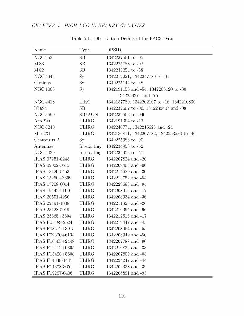
CHAPTER 5. HIGH-J CO IN NEARBY GALAXIES
Table 5.1:: Observation Details of the PACS Data
Name Type OBSID
NGC 253 SB 1342237601 to -05
M 83 SB 1342225788 to -92
M 82 SB 1342232254 to -58
NGC 4945 Sy 1342212221, 1342247789 to -91
Circinus Sy 1342225144 to -48
NGC 1068 Sy 1342191153 and -54, 1342203120 to -30,
1342239374 and -75
NGC 4418 LIRG 1342187780, 1342202107 to -16, 1342210830
IC 694 SB 1342232602 to -06, 1342232607 and -08
NGC 3690 SB/AGN 1342232602 to -046
Arp 220 ULIRG 1342191304 to -13
NGC 6240 ULIRG 1342240774, 1342216623 and -24
Mrk 231 ULIRG 1342186811, 1342207782, 1342253530 to -40
Centaurus A Sy 1342225986 to -90
Antennae Interacting 1342234958 to -62
NGC 4039 Interacting 1342234953 to -57
IRAS 07251-0248 ULIRG 1342207824 and -26
IRAS 09022-3615 ULIRG 1342209403 and -06
IRAS 13120-5453 ULIRG 1342214629 and -30
IRAS 15250+3609 ULIRG 1342213752 and -54
IRAS 17208-0014 ULIRG 1342229693 and -94
IRAS 19542+1110 ULIRG 1342208916 and -17
IRAS 20551-4250 ULIRG 1342208934 and -36
IRAS 22491-1808 ULIRG 1342211825 and -26
IRAS 23128-5919 ULIRG 1342210395 and -96
IRAS 23365+3604 ULIRG 1342212515 and -17
IRAS F05189-2524 ULIRG 1342219442 and -45
IRAS F08572+3915 ULIRG 1342208954 and -55
IRAS F09320+6134 ULIRG 1342208949 and -50
IRAS F10565+2448 ULIRG 1342207788 and -90
IRAS F12112+0305 ULIRG 1342210832 and -33
IRAS F13428+5608 ULIRG 1342207802 and -03
IRAS F14348-1447 ULIRG 1342224242 and -44
IRAS F14378-3651 ULIRG 1342204338 and -39
IRAS F19297-0406 ULIRG 1342208891 and -93
110
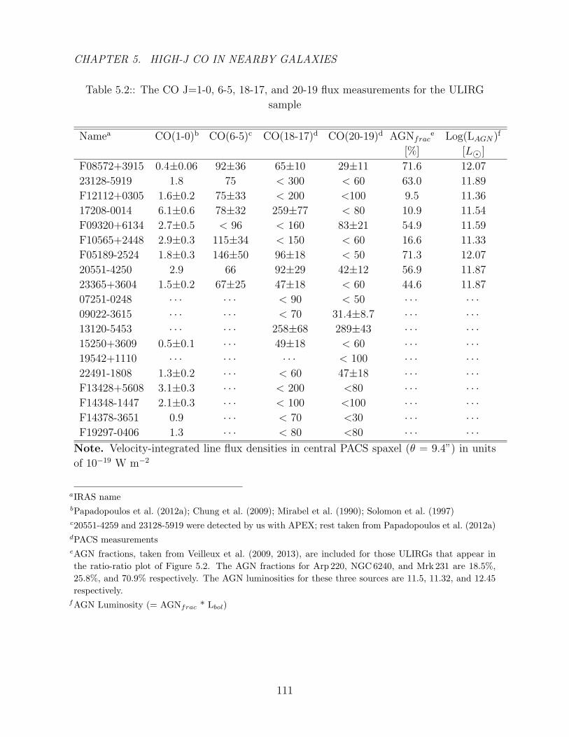
CHAPTER 5. HIGH-J CO IN NEARBY GALAXIES
Table 5.2:: The CO J=1-0, 6-5, 18-17, and 20-19 flux measurements for the ULIRG
sample
Namea CO(1-0)b CO(6-5)c CO(18-17)d CO(20-19)d AGNfrace Log(LAGN )f
[%] [L]
F08572+3915 0.4±0.06 92±36 65±10 29±11 71.6 12.07
23128-5919 1.8 75 < 300 < 60 63.0 11.89
F12112+0305 1.6±0.2 75±33 < 200 <100 9.5 11.36
17208-0014 6.1±0.6 78±32 259±77 < 80 10.9 11.54
F09320+6134 2.7±0.5 < 96 < 160 83±21 54.9 11.59
F10565+2448 2.9±0.3 115±34 < 150 < 60 16.6 11.33
F05189-2524 1.8±0.3 146±50 96±18 < 50 71.3 12.07
20551-4250 2.9 66 92±29 42±12 56.9 11.87
23365+3604 1.5±0.2 67±25 47±18 < 60 44.6 11.87
07251-0248 · · · · · · < 90 < 50 · · · · · ·09022-3615 · · · · · · < 70 31.4±8.7 · · · · · ·13120-5453 · · · · · · 258±68 289±43 · · · · · ·15250+3609 0.5±0.1 · · · 49±18 < 60 · · · · · ·19542+1110 · · · · · · · · · < 100 · · · · · ·22491-1808 1.3±0.2 · · · < 60 47±18 · · · · · ·F13428+5608 3.1±0.3 · · · < 200 <80 · · · · · ·F14348-1447 2.1±0.3 · · · < 100 <100 · · · · · ·F14378-3651 0.9 · · · < 70 <30 · · · · · ·F19297-0406 1.3 · · · < 80 <80 · · · · · ·
Note. Velocity-integrated line flux densities in central PACS spaxel (θ = 9.4”) in units
of 10−19 W m−2
aIRAS namebPapadopoulos et al. (2012a); Chung et al. (2009); Mirabel et al. (1990); Solomon et al. (1997)c20551-4259 and 23128-5919 were detected by us with APEX; rest taken from Papadopoulos et al. (2012a)dPACS measurementseAGN fractions, taken from Veilleux et al. (2009, 2013), are included for those ULIRGs that appear in
the ratio-ratio plot of Figure 5.2. The AGN fractions for Arp 220, NGC 6240, and Mrk 231 are 18.5%,
25.8%, and 70.9% respectively. The AGN luminosities for these three sources are 11.5, 11.32, and 12.45
respectively.fAGN Luminosity (= AGNfrac * Lbol)
111
CHAPTER 5. HIGH-J CO IN NEARBY GALAXIES
For the final calibration we normalized the spectra to the telescope flux and recalibrated
it with a reference telescope spectrum obtained from dedicated Neptune continuum
observations. This ‘background normalization’ method is described in the PACS
data reduction guide. We also assessed the line flux uncertainties associated with the
uncertainties in defining the continuum and estimated an absolute line flux accuracy of
20% with this method.
The PACS spectrometer performs integral field spectroscopy over a 47” × 47” FoV,
resolved into a 5 × 5 array of 9.4” spatial pixels (spaxels.) With the exception of M 83,
M 82, and NGC 3690, the high-J lines in the PACS range for the remaining sources are
all consistent with arising in the central spaxel, with little, if any, flux detected outside
of the central spaxel. The fluxes were thus extracted from the central spaxel only (θ =
9.4”), and referenced to a point source by dividing by the recommended point source
correction factors as given in the PACS manual. We did spot checks with HIPE 11 and
verified that this does not yield significantly different line fluxes or upper limits.
In the case of M 83 and M 82 where the high-J CO emission are extended beyond
the central spaxel, the fluxes were derived by integrating over the entire PACS FoV. For
NGC 3690, the PACS flux measurements cover both the galaxy, as well as an extended
region of star formation where the galaxy disks of NGC 3690 and IC 694 overlap. The
high-J line fluxes for this source were thus derived by co-adding the 3 spaxels covering
components B and C (as NGC 3690 and the overlap region are respectively referred to in
the literature).
To supplement these PACS line observations, we collect low and mid-J line fluxes for
these sources from the literature and, when necessary, apply aperture corrections using
112
CHAPTER 5. HIGH-J CO IN NEARBY GALAXIES
available CO maps. For point-like sources such as Arp 220, NGC 6240, and Mrk 231,
where the low and mid-J line fluxes are fully contained in the PACS beam, no aperture
corrections are necessary. This is also deemed to be the case for NGC 4418 and IC 694,
where 12CO J=1-0, J=2-1, and J=3-2 maps reveal the emission to be fully enclosed
within a θ ∼ 10” beam (Sakamoto et al. 2013; Sliwa et al. 2012; Casoli et al. 1999). The
morphology of NGC 1068, which is composed of a compact central circumnuclear disk
(θ ∼ 4”) and an extended ring (θ ∼ 20-40”), is slightly more complex. To avoid potential
scaling issues, we only consider lines that are probed on the scale of the compact source
at the center of NGC 1068, i.e. the interferometric measurements of the Jupp = 1 - 3 lines
integrated over the central 4” by Krips et al. (2011), and the Jupp = 9 - 13 lines probed
by SPIRE FTS with a beam width of θ ∼ 17” (Spinoglio et al. 2012).
In the case of M 83, aperture corrections are also deemed unnecessary since PACS
flux measurements for this source extend over a ∼ 21” area, and the low and mid-J lines
found in the literature refer to a similar beam size (Bayet et al. 2006; Israel & Baas
2001). Similarly, for M 82, the Jupp = 4 - 13 12CO lines are referenced to the ∼ 43” beam
size of the SPIRE spectrometer (Kamenetzky et al. 2012) and therefore do not need to
be scaled when compared against the high-J lines which fill the PACS FoV (θ = 47”) in
this source. The 12CO J=1-0 map for M 82 indicates that the low-J lines are also not in
need of any scaling corrections since the emission is predominately contained within an
∼25” area, consistent with the FWHP beam of 24.4” referenced for the Jupp = 1 - 3 line
measurements (Ward et al. 2003).
12CO J=1-0, J=2-1, and J=3-2 maps for the Arp 299 merger system show that the
source sizes of NGC 3690 and the overlap region are θ ∼ 2” and 4” respectively, and that
the combined emission from these two components does not extend beyond θ ∼ 19” (the
113

CHAPTER 5. HIGH-J CO IN NEARBY GALAXIES
PACS aperture size over which the high-J lines were integrated) (Sliwa et al. 2012). The
low-J line fluxes for this region are thus derived by co-adding the flux values presented
in the literature for components B and C without any further scaling corrections. The
mid-J line fluxes are taken from SPIRE observations which include contributions from
both components, B and C (Rosenberg et al. 2014b). Although the SPIRE beam sizes
vary (15-42”), it is assumed that the fluxes, too, are mostly contained within a 19” beam
and no further scaling is applied.
In the case of NGC 4945 and Circinus, available CO maps of the low-J lines indicate
that these sources are spatially resolved and more extended than the PACS single spaxel
size (Dahlem et al. 1993; Mauersberger et al. 1996; Curran et al. 2008; Zhang et al. 2014).
Since the recorded fluxes fill the respective beams with which they were probed, we
assume a uniform distribution of flux and linearly scale the low-J emission with the ratio
of the PACS spaxel area and the respective literature beam area. A similar technique is
applied to NGC 253, where the extended low and mid-J lines corrected to a 15” beam
are assumed to be uniformly distributed over that beam size and are thus scaled linearly
with the PACS area (Rosenberg et al. 2014a; Hailey-Dunsheath et al. 2008).
The PACS measurements, along with the (aperture-corrected) low-J line fluxes
collected from the literature, are summarized in Tables 5.3 and 5.4.
114
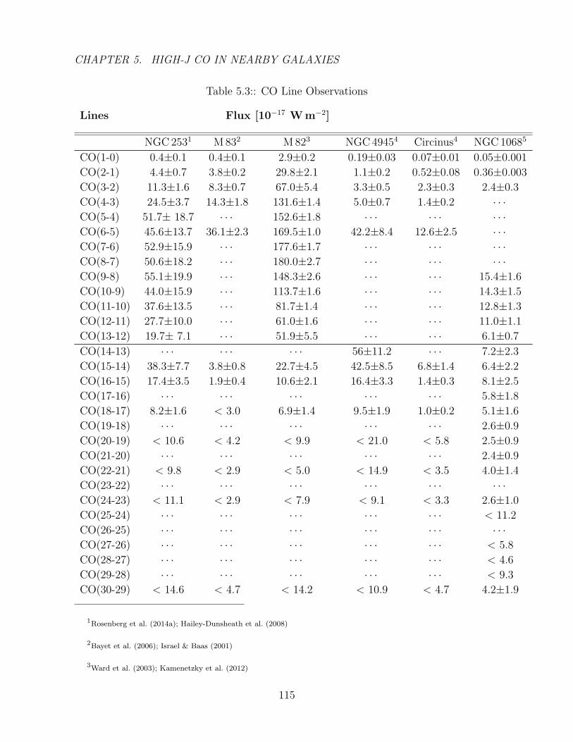
CHAPTER 5. HIGH-J CO IN NEARBY GALAXIES
Table 5.3:: CO Line Observations
Lines Flux [10−17 Wm−2]
NGC 2531 M 832 M 823 NGC 49454 Circinus4 NGC 10685
CO(1-0) 0.4±0.1 0.4±0.1 2.9±0.2 0.19±0.03 0.07±0.01 0.05±0.001
CO(2-1) 4.4±0.7 3.8±0.2 29.8±2.1 1.1±0.2 0.52±0.08 0.36±0.003
CO(3-2) 11.3±1.6 8.3±0.7 67.0±5.4 3.3±0.5 2.3±0.3 2.4±0.3
CO(4-3) 24.5±3.7 14.3±1.8 131.6±1.4 5.0±0.7 1.4±0.2 · · ·CO(5-4) 51.7± 18.7 · · · 152.6±1.8 · · · · · · · · ·CO(6-5) 45.6±13.7 36.1±2.3 169.5±1.0 42.2±8.4 12.6±2.5 · · ·CO(7-6) 52.9±15.9 · · · 177.6±1.7 · · · · · · · · ·CO(8-7) 50.6±18.2 · · · 180.0±2.7 · · · · · · · · ·CO(9-8) 55.1±19.9 · · · 148.3±2.6 · · · · · · 15.4±1.6
CO(10-9) 44.0±15.9 · · · 113.7±1.6 · · · · · · 14.3±1.5
CO(11-10) 37.6±13.5 · · · 81.7±1.4 · · · · · · 12.8±1.3
CO(12-11) 27.7±10.0 · · · 61.0±1.6 · · · · · · 11.0±1.1
CO(13-12) 19.7± 7.1 · · · 51.9±5.5 · · · · · · 6.1±0.7
CO(14-13) · · · · · · · · · 56±11.2 · · · 7.2±2.3
CO(15-14) 38.3±7.7 3.8±0.8 22.7±4.5 42.5±8.5 6.8±1.4 6.4±2.2
CO(16-15) 17.4±3.5 1.9±0.4 10.6±2.1 16.4±3.3 1.4±0.3 8.1±2.5
CO(17-16) · · · · · · · · · · · · · · · 5.8±1.8
CO(18-17) 8.2±1.6 < 3.0 6.9±1.4 9.5±1.9 1.0±0.2 5.1±1.6
CO(19-18) · · · · · · · · · · · · · · · 2.6±0.9
CO(20-19) < 10.6 < 4.2 < 9.9 < 21.0 < 5.8 2.5±0.9
CO(21-20) · · · · · · · · · · · · · · · 2.4±0.9
CO(22-21) < 9.8 < 2.9 < 5.0 < 14.9 < 3.5 4.0±1.4
CO(23-22) · · · · · · · · · · · · · · · · · ·CO(24-23) < 11.1 < 2.9 < 7.9 < 9.1 < 3.3 2.6±1.0
CO(25-24) · · · · · · · · · · · · · · · < 11.2
CO(26-25) · · · · · · · · · · · · · · · · · ·CO(27-26) · · · · · · · · · · · · · · · < 5.8
CO(28-27) · · · · · · · · · · · · · · · < 4.6
CO(29-28) · · · · · · · · · · · · · · · < 9.3
CO(30-29) < 14.6 < 4.7 < 14.2 < 10.9 < 4.7 4.2±1.9
1Rosenberg et al. (2014a); Hailey-Dunsheath et al. (2008)
2Bayet et al. (2006); Israel & Baas (2001)
3Ward et al. (2003); Kamenetzky et al. (2012)
115
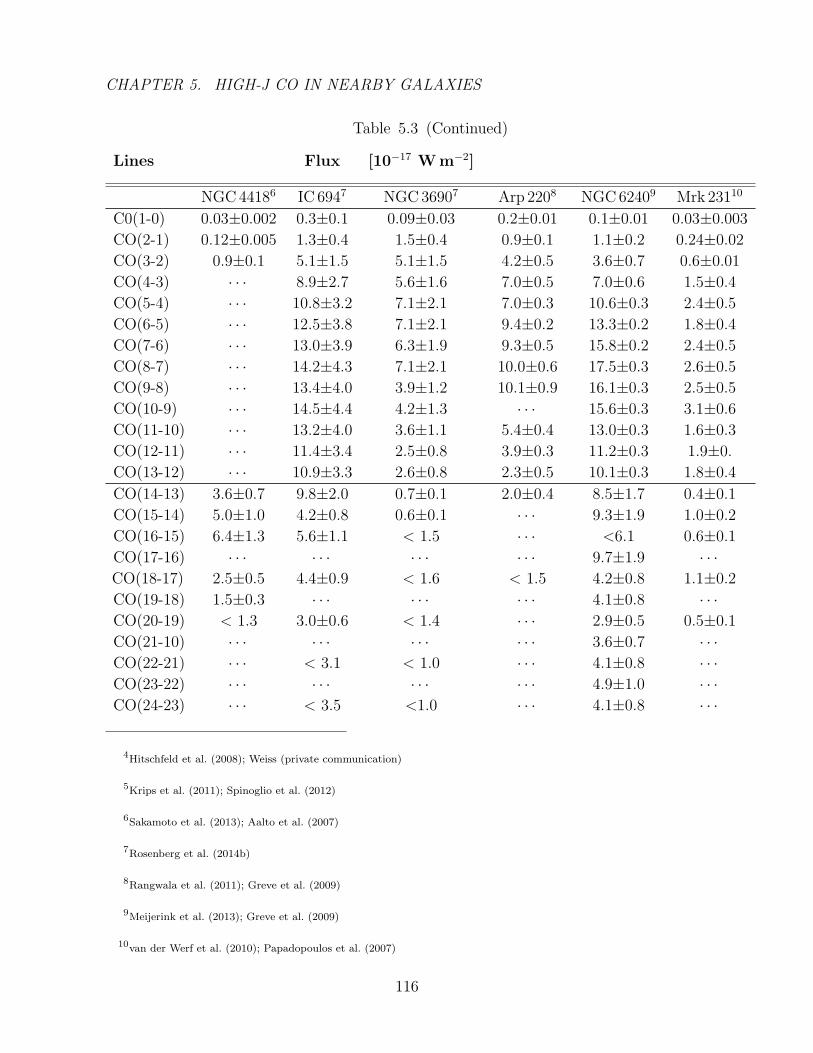
CHAPTER 5. HIGH-J CO IN NEARBY GALAXIES
Table 5.3 (Continued)
Lines Flux [10−17 Wm−2]
NGC 44186 IC 6947 NGC 36907 Arp 2208 NGC 62409 Mrk 23110
C0(1-0) 0.03±0.002 0.3±0.1 0.09±0.03 0.2±0.01 0.1±0.01 0.03±0.003
CO(2-1) 0.12±0.005 1.3±0.4 1.5±0.4 0.9±0.1 1.1±0.2 0.24±0.02
CO(3-2) 0.9±0.1 5.1±1.5 5.1±1.5 4.2±0.5 3.6±0.7 0.6±0.01
CO(4-3) · · · 8.9±2.7 5.6±1.6 7.0±0.5 7.0±0.6 1.5±0.4
CO(5-4) · · · 10.8±3.2 7.1±2.1 7.0±0.3 10.6±0.3 2.4±0.5
CO(6-5) · · · 12.5±3.8 7.1±2.1 9.4±0.2 13.3±0.2 1.8±0.4
CO(7-6) · · · 13.0±3.9 6.3±1.9 9.3±0.5 15.8±0.2 2.4±0.5
CO(8-7) · · · 14.2±4.3 7.1±2.1 10.0±0.6 17.5±0.3 2.6±0.5
CO(9-8) · · · 13.4±4.0 3.9±1.2 10.1±0.9 16.1±0.3 2.5±0.5
CO(10-9) · · · 14.5±4.4 4.2±1.3 · · · 15.6±0.3 3.1±0.6
CO(11-10) · · · 13.2±4.0 3.6±1.1 5.4±0.4 13.0±0.3 1.6±0.3
CO(12-11) · · · 11.4±3.4 2.5±0.8 3.9±0.3 11.2±0.3 1.9±0.
CO(13-12) · · · 10.9±3.3 2.6±0.8 2.3±0.5 10.1±0.3 1.8±0.4
CO(14-13) 3.6±0.7 9.8±2.0 0.7±0.1 2.0±0.4 8.5±1.7 0.4±0.1
CO(15-14) 5.0±1.0 4.2±0.8 0.6±0.1 · · · 9.3±1.9 1.0±0.2
CO(16-15) 6.4±1.3 5.6±1.1 < 1.5 · · · <6.1 0.6±0.1
CO(17-16) · · · · · · · · · · · · 9.7±1.9 · · ·CO(18-17) 2.5±0.5 4.4±0.9 < 1.6 < 1.5 4.2±0.8 1.1±0.2
CO(19-18) 1.5±0.3 · · · · · · · · · 4.1±0.8 · · ·CO(20-19) < 1.3 3.0±0.6 < 1.4 · · · 2.9±0.5 0.5±0.1
CO(21-10) · · · · · · · · · · · · 3.6±0.7 · · ·CO(22-21) · · · < 3.1 < 1.0 · · · 4.1±0.8 · · ·CO(23-22) · · · · · · · · · · · · 4.9±1.0 · · ·CO(24-23) · · · < 3.5 <1.0 · · · 4.1±0.8 · · ·
4Hitschfeld et al. (2008); Weiss (private communication)
5Krips et al. (2011); Spinoglio et al. (2012)
6Sakamoto et al. (2013); Aalto et al. (2007)
7Rosenberg et al. (2014b)
8Rangwala et al. (2011); Greve et al. (2009)
9Meijerink et al. (2013); Greve et al. (2009)
10van der Werf et al. (2010); Papadopoulos et al. (2007)
116
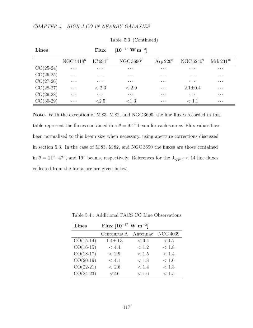
CHAPTER 5. HIGH-J CO IN NEARBY GALAXIES
Table 5.3 (Continued)
Lines Flux [10−17 Wm−2]
NGC 44186 IC 6947 NGC 36907 Arp 2208 NGC 62409 Mrk 23110
CO(25-24) · · · · · · · · · · · · · · · · · ·CO(26-25) · · · · · · · · · · · · · · · · · ·CO(27-26) · · · · · · · · · · · · · · · · · ·CO(28-27) · · · < 2.3 < 2.9 · · · 2.1±0.4 · · ·CO(29-28) · · · · · · · · · · · · · · · · · ·CO(30-29) · · · <2.5 <1.3 · · · < 1.1 · · ·
Note. With the exception of M 83, M 82, and NGC 3690, the line fluxes recorded in this
table represent the fluxes contained in a θ = 9.4” beam for each source. Flux values have
been normalized to this beam size when necessary, using aperture corrections discussed
in section 5.3. In the case of M 83, M 82, and NGC 3690 the fluxes are those contained
in θ = 21”, 47”, and 19” beams, respectively. References for the Jupper < 14 line fluxes
collected from the literature are given below.
Table 5.4:: Additional PACS CO Line Observations
Lines Flux [10−17 W m−2]
Centaurus A Antennae NCG 4039
CO(15-14) 1.4±0.3 < 0.4 <0.5
CO(16-15) < 4.4 < 1.2 < 1.8
CO(18-17) < 2.9 < 1.5 < 1.4
CO(20-19) < 4.1 < 1.8 < 1.6
CO(22-21) < 2.6 < 1.4 < 1.3
CO(24-23) <2.6 < 1.6 < 1.5
117
CHAPTER 5. HIGH-J CO IN NEARBY GALAXIES
5.4 Excitation Analysis
5.4.1 CO SLEDs and Line Ratios
The observed CO SLEDs of the sources, whose excitation conditions will further be
explored in the following sections, display a large variation in overall SLED shapes
(Figure 5.1). On a first glance this spread seems to nicely follow the qualitatively
expected behavior that the strength of high-J CO lines increases with increasing
importance of an AGN in these sources. For instance, the CO SLED of the archetypal
starburst galaxy M 82 peaks at around Jupp = 7 and then quickly declines towards
higher J values, while the archetypical Seyfert 2 galaxy NGC 1068 shows strong CO
lines even above Jupp = 20. In Mrk 231, the CO SLED rises up to Jupp = 5 and then
remains relatively flat for the higher-J transitions, consistent with the presence of a
central X-ray source illuminating the circumnuclear region. However, other sources
do not seem to follow the expected trends. The starburst galaxy NGC 253 and the
ULIRG NGC 6240, a mixed source thought to be less dominated by its AGN than e.g.
Mrk 231 (based on mid-IR diagnostics) exhibit extremely strong high-J lines, suggesting
that other excitation sources, like warm PDRs (as in NGC 253) or strong shocks (as in
NGC 6240) have to be considered as well, i.e. that the pure detection of a high-J CO line
alone is not an unambiguous signature of an XDR excited by an AGN. In a previous
paper (Hailey-Dunsheath et al. 2012), we showed that the well characterized SLED of
NGC 1068 could not be uniquely explained with a mixture of PDR, XDR, and shock
models. It was only with additional information that an AGN could be identified as the
most likely excitation source of the highly excited components. Our new findings here,
drawn from a much larger sample, underline the importance of this caveat.
118
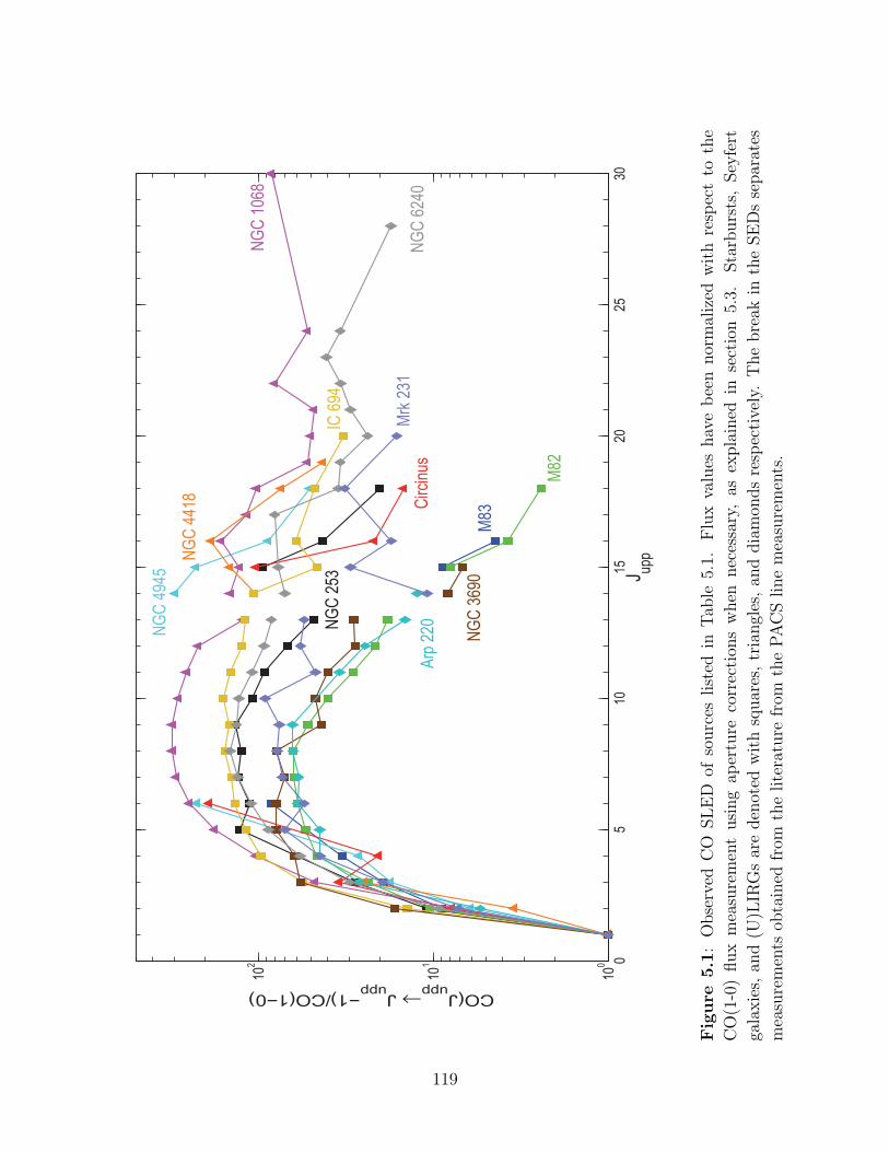
CHAPTER 5. HIGH-J CO IN NEARBY GALAXIES
05
1015
2025
3010
0
101
102
NG
C 2
53
M83
M82
NG
C 4
945
Circ
inus
NG
C 1
068
NG
C 4
418
IC 6
94
NG
C 3
690
Arp
220
NG
C 6
240
Mrk
231
CO(Jupp
→ Jupp
−1)/CO(1−0)
J upp
Figure
5.1
:O
bse
rved
CO
SL
ED
ofso
urc
eslist
edin
Tab
le5.
1.F
lux
valu
eshav
eb
een
nor
mal
ized
wit
hre
spec
tto
the
CO
(1-0
)flux
mea
sure
men
tusi
ng
aper
ture
corr
ecti
ons
when
nec
essa
ry,
asex
pla
ined
inse
ctio
n5.
3.Sta
rburs
ts,
Sey
fert
gala
xie
s,an
d(U
)LIR
Gs
are
den
oted
wit
hsq
uar
es,
tria
ngl
es,
and
dia
mon
ds
resp
ecti
vely
.T
he
bre
akin
the
SE
Ds
separ
ates
mea
sure
men
tsob
tain
edfr
omth
elite
ratu
refr
omth
eP
AC
Sline
mea
sure
men
ts.
119

CHAPTER 5. HIGH-J CO IN NEARBY GALAXIES
The implication of these findings is particularly relevant in studies of high-redshift
galaxies, where the majority of CO detections are limited to high-J transitions. The
findings in this paper demonstrate the difficulty in applying high-J CO diagnostics in
a simple manner to identify XDRs/AGNs in dusty high-redshift sources. In particular,
if only a single or a few CO lines are observed, without a broad coverage of the entire
SLED, these line detections can be misinterpreted.
Furthermore, caution must be exercised in calculations of the total molecular gas
mass via the so-called CO-to-H2 conversion factor, αCO = MH2/LCO(1−0), (e.g. expressed
in units of M/(K km s−1 pc2)). Since at high redshifts, CO detections are limited to J
> 3 lines, many studies are forced to first convert an observed mid-J CO line intensity
to a J = 1→ 0 intensity before applying αCO to arrive at an H2 gas mass. Usually, line
ratios between a mid-J or high-J line and the J = 1→0 line are estimated by comparing
the source to a similar galaxy and assuming the typical excitation of the galaxy under
consideration (Carilli & Walter 2013). However, the diversity in our observed SLEDs
(Figure 5.1) suggests that this approach may be problematic; extrapolating from mid or
high-J lines to J = 1→0 using templates based on galaxies with similar inferred physical
properties introduces a degree of uncertainty since the high-J to CO(1-0) line ratios can
vary by an order of magnitude for otherwise similar sources.
In order to further explore the usefulness of high-J CO lines as a tool for
characterizing dusty objects at high redshifts, we construct a ratio-ratio diagram
employing just three CO lines: J = 1→0, 6→5, and 18→17. The CO(1-0) transition is
traditionally used to trace the total molecular gas mass, while the CO(6-5) line traces
a warm and dense component that is generally associated with star formation, and is
typically one of the brightest transitions in infrared-bright starburst galaxies (see Figure
120
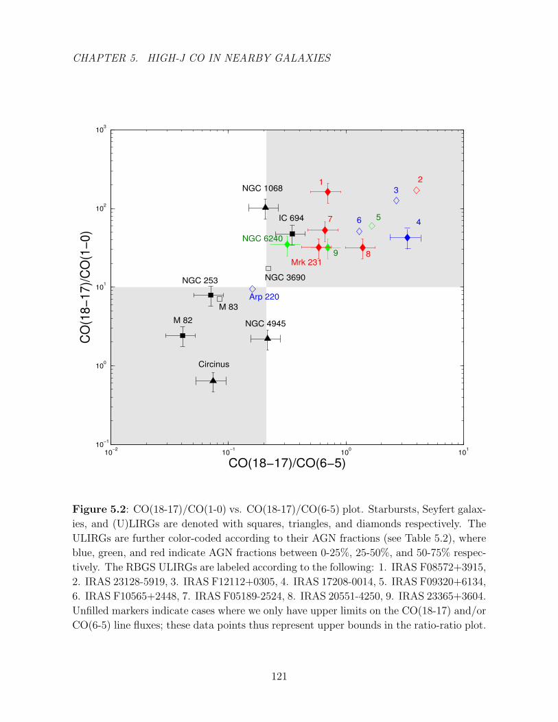
CHAPTER 5. HIGH-J CO IN NEARBY GALAXIES
CO
(18
−1
7)/
CO
(1−
0)
CO(18−17)/CO(6−5)
10−2
10−1
100
101
10−1
100
101
102
103
1 2
3
4567
89
Mrk 231
IC 694
NGC 1068
NGC 6240
NGC 3690
Arp 220
NGC 4945
M 83
NGC 253
M 82
Circinus
Figure 5.2: CO(18-17)/CO(1-0) vs. CO(18-17)/CO(6-5) plot. Starbursts, Seyfert galax-
ies, and (U)LIRGs are denoted with squares, triangles, and diamonds respectively. The
ULIRGs are further color-coded according to their AGN fractions (see Table 5.2), where
blue, green, and red indicate AGN fractions between 0-25%, 25-50%, and 50-75% respec-
tively. The RBGS ULIRGs are labeled according to the following: 1. IRAS F08572+3915,
2. IRAS 23128-5919, 3. IRAS F12112+0305, 4. IRAS 17208-0014, 5. IRAS F09320+6134,
6. IRAS F10565+2448, 7. IRAS F05189-2524, 8. IRAS 20551-4250, 9. IRAS 23365+3604.
Unfilled markers indicate cases where we only have upper limits on the CO(18-17) and/or
CO(6-5) line fluxes; these data points thus represent upper bounds in the ratio-ratio plot.
121
CHAPTER 5. HIGH-J CO IN NEARBY GALAXIES
5.1). CO(18-17) is a very high-J line that may offer a large leverage in distinguishing
starburst-dominated from AGN-dominated excitation. Figure 5.2 shows the resulting
plot of the CO(18-17)/CO(1-0) versus CO(18-17)/CO(6-5) ratios in cases where flux
values (or upper limits) for all three rotational lines are available. Since Figure 5.2 is
meant to serve as an observational tool, we plot ratios of the observed (unscaled) flux
values, as opposed to the line fluxes plotted in Figure 5.1 and tabulated in Table 5.3,
which have been scaled to the PACS 9.4” beam size when necessary. (A scaled version of
Figure 5.2 demonstrates the same qualitative trends discussed below.)
We find that the CO(18-17) line is weak with respect to both CO(1-0) and CO(6-5)
in our starburst galaxies (NGC 253, M 83, M 82), and strong in the prototypical Seyfert
NGC 1068 and in the ULIRGs of our sample, which are generally located in a region
above the starbursts, in the upper right corner where objects have significant amounts of
hot gas. A quantitative treatment of this trend will be presented in section 5.5.
We also searched for potential trends between the ULIRG positions in this diagram
and their AGN properties. We collected the AGN luminosities and AGN fractions, i.e. the
relative contribution of the AGN (w.r.t. the starburst) to the combined bolometric light
in these objects (taken from Veilleux et al. (2009, 2013) and listed in Table 5.2), but did
not find a clear trend with either of these two parameters.
5.4.2 LVG Radiative Transfer Model
To quantitatively analyze the CO SLEDs of the sources in our sample, we assemble
the lower-J line intensities from the literature (see footnotes in Table 5.3) and employ
a large velocity gradient (LVG) model in which the excitation and opacity of the CO
122
CHAPTER 5. HIGH-J CO IN NEARBY GALAXIES
lines are determined by the gas density (nH2), kinetic temperature (Tkin), and the
CO-to-H2 abundance per velocity gradient (χCO/(dv/dr)). We use the escape probability
formalism derived for a spherical cloud undergoing uniform collapse, with β = (1-e−τ )/τ
(Castor 1970; Goldreich & Kwan 1974). Each source is assumed to consist of a large
number of these unresolved clouds, such that the absolute line intensities scale with
the beam-averaged CO column density, NCO. In the following analysis, we assume a
canonical value of χCO = 10−4, motivated by abundance measurements in Galactic
molecular clouds (Frerking et al. 1982). We assume collisional excitation by H2 assuming
an H2 ortho/para ratio of 3.
To carry out the computations, we use the Mark & Sternberg LVG radiative
transfer code described in Davies et al. (2012), with CO-H2 collisional coefficients taken
from Yang et al. (2010) and energy levels, line frequencies and Einstein A coefficients
taken from the Cologne Database for Molecular Spectroscopy (CDMS). For a given
set of parameters, nH2 , Tkin, dv/dr, NCO, the code computes the intensities of
molecular lines by iteratively solving the equations of statistical equilibrium for the level
populations using the escape probability formalism. We calculate a three-dimensional
grid of expected CO SLEDs, varying nH2 (102.4-108.2 cm−3), Tkin (30-2500 K), and dv/dr
(0.1-1000 km s−1pc−1) over a large volume of parameter space. While these parameters
determine the shape of the resulting SLED, the line intensity magnitudes are set by the
beam-averaged CO column density, NCO, which is tweaked to match the observed fluxes
and beam sizes. Thus the intensity of each CO line is given by the expression
Iline =hν
4πxuAβ(τ)NCO (5.1)
where xu is the population fraction in the upper level of the transition, hν is the
123

CHAPTER 5. HIGH-J CO IN NEARBY GALAXIES
transition energy, A is the Einstein radiative coefficient, β(τ) is the escape probability for
a line optical depth τ , and NCO is the beamed averaged column density. The molecular
gas mass in the beam (for a spherical geometry) is then given by
MH2 = πR2µmH2
NCO
χCO(5.2)
where µ = 1.36 takes into account the helium contribution to the molecular weight and
R = DAθ/2 is the effective radius of the beam, with DA being the angular diameter
distance to the source and θ the beam size of the line observations.
The LVG-modeling technique thus offers an opportunity to derive the CO-to-H2
conversion factor in an extragalactic source in an independent way, using the gas mass
estimate from the source’s best-fit LVG model (Mashian et al. 2013). As mentioned
above, the molecular hydrogen gas mass is often obtained from the CO(1-0) line
luminosity by adopting a mass-to-luminosity conversion factor, αCO. The standard
Galactic value, calibrated using several independent methods (Dickman 1978; Bloemen
et al. 1986; Solomon et al. 1987; Strong et al. 1988), is αCO ∼ 4 - 5 M/(K km−1pc2),
while subsequent studies of CO emission in ULIRGs found a significantly smaller ratio,
αCO ∼ 0.8 - 1.0 M/(K km−1pc2) (Downes & Solomon 1998). These values have been
adopted by many (Sanders et al. 1988; Tinney et al. 1990; Wang et al. 1991; Walter
et al. 2012) to convert CO J=1-0 line observations to total molecular gas masses, and the
question of what value to apply for what type of galaxy has been a controversial issue
for decades. Often, consideration is not given to the dependence of αCO on the average
molecular gas conditions (metallicity, temperature, density) in the sources to which they
are being applied.
Detailed studies of the conversion factor based on CO SLED modeling of the
124
CHAPTER 5. HIGH-J CO IN NEARBY GALAXIES
objects in our sample are beyond the scope of this paper because of the significant
uncertainties associated with our simple models. We do estimate, however, the conversion
factors derived using the LCO(1−0) and MH2 values from both the single-component and
two-component LVG models for each of the sources in our sample (where the total
gas mass, MH2,total = MH2,cool + MH2,warm, is used in the two-component case). We
note that the sole use of 12CO lines to derive the CO-to-H2 conversion factor via LVG
modeling raises its own concerns. As discussed in Bolatto et al. (2013), this technique
is only sensitive to regions where CO is bright and may therefore miss any component
of “CO-faint” H2, unless combined with observations of other lines, i.e. [CII], that trace
these “CO-faint” molecular regions.
5.4.3 Fitting Procedure
To determine the best-fit set of parameters that characterize the CO SLED of each
source, we compare the modeled SLEDs to the observed CO line intensities and generate
a likelihood distribution for each of the parameters following a Bayesian formalism
outlined in Ward et al. (2003) and Kamenetzky et al. (2012). The Bayesian likelihood of
the model parameters, p, given the line measurements, x , is
P (p|x ) =P (p)P (x |p)∫dpP (p)P (x |p)
(5.3)
where P (p) is the prior probability of the model parameters and P (x |p) is the probability
of obtaining the observed data set given that the source follows the model characterized
by p. Assuming that the measured line strengths have Gaussian-distributed random
125

CHAPTER 5. HIGH-J CO IN NEARBY GALAXIES
errors, P (x |p) is the product of Gaussian distributions in each observation,
P (x |p) =∏i
1√2πσ2
i
exp
[−(xi − Ii(p))2
2σ2i
](5.4)
where σi is the standard deviation of the observational measurement for transition i
and Ii(p) is the predicted line intensity for that transition and model. The likelihood
distribution of any one parameter is thus the integral of P (p|x ) over all the other
parameters. In our analysis, we use a binary prior probability, choosing priors that are
flat in the logarithm of each parameter, and that go to zero for any model that predicts
a molecular gas mass which exceeds the source’s dynamical mass (in cases where Mdyn is
known through other means; see footnote in Table 5.5).
We first run a calculation with a single-component model, assuming all the CO
lines are emitted by a region characterized by a single kinetic temperature, H2 number
density, velocity gradient, and column density. It is instructive to examine how far a
single gas component can go in reproducing the entire observed CO SLEDs before a
given fit becomes inadequate and a second component must be introduced. However,
given the fact that many of the sources considered in this paper have had their low- to
mid-J emission lines analyzed in previous studies (see Table 5.6) using two-component
LVG models, we would like to explore how these “best-fit” multi-component models
are modified by the inclusion of the more recent PACS high-J line observations. We
therefore divide the line fluxes into two components, one cooler and one warmer (with
some mid-J lines receiving significant contributions from both) and follow an iterative
procedure, looking for the best solution of one component at a time and subtracting it
from the other. This two-step approach thus results in a six parameter model, with three
parameters characterizing the shape of the SLED in each respective component. It is
126
CHAPTER 5. HIGH-J CO IN NEARBY GALAXIES
therefore not applied to sources which have fewer than three line intensity measurements
in each component, i.e. M 83, since in such cases, the problem is underdetermined, i.e.
there are more parameters than data points. The detected transitions from NGC 1068
are also not modeled as arising from two different components in this paper since the
full SLED has been thoroughly analyzed and fitted with radiative transfer models in
previous papers (Hailey-Dunsheath et al. 2012; Spinoglio et al. 2012).
5.5 LVG Results & Discussion
The LVG-modeled SLEDs for the single and two-component fits are shown in the left and
right-hand panels of Figure 5.3 respectively. Although the single-component LVG models
provide only a crude approximation to the complicated mixture of physical conditions
that characterize the emitting source, they nonetheless yield surprisingly good fits to
the observed SLEDs in most cases. The constraints provided by the PACS high-J CO
line detections drive the “best-fit” kinetic temperatures in these single component LVG
models to high values, both relative to their two-component counterparts and relative to
CO SLED fits obtained in earlier LVG analyses, when measurements of these high-level
excitations were not yet available. Furthermore, demanding that a single set of LVG
model parameters reproduce the full CO SLED often results in under-predicted low-J
CO transitions. Introducing a separate low-excitation component mitigates both of these
issues, accounting for the excess CO(1-0) and CO(2-1) line emissions while yielding a
two-component LVG model with more moderate estimates of the kinetic temperature.
While a true multi-component model will obviously provide more accurate estimates of
these molecular gas properties, the fact that in most cases, a single component LVG
127
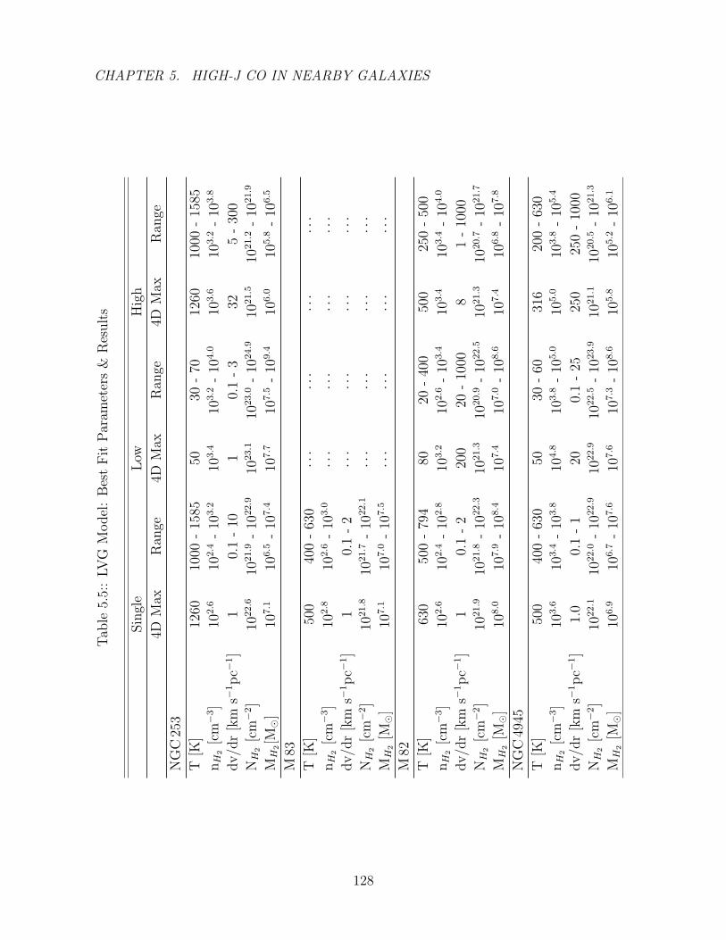
CHAPTER 5. HIGH-J CO IN NEARBY GALAXIES
Tab
le5.
5::
LV
GM
odel
:B
est
Fit
Par
amet
ers
&R
esult
s
Sin
gle
Low
Hig
h
4DM
axR
ange
4DM
axR
ange
4DM
axR
ange
NG
C25
3
T[K
]12
6010
00-
1585
5030
-70
1260
1000
-15
85
nH
2[c
m−
3]
102.6
102.4
-10
3.2
103.4
103.2
-10
4.0
103.6
103.2
-10
3.8
dv/d
r[k
ms−
1p
c−1]
10.
1-
101
0.1
-3
325
-30
0
NH
2[c
m−
2]
1022.6
1021.9
-10
22.9
1023.1
1023.0
-10
24.9
1021.5
1021.2
-10
21.9
MH
2[M
]10
7.1
106.5
-10
7.4
107.7
107.5
-10
9.4
106.0
105.8
-10
6.5
M83
T[K
]50
040
0-
630
···
···
···
···
nH
2[c
m−
3]
102.8
102.6
-10
3.0
···
···
···
···
dv/d
r[k
ms−
1p
c−1]
10.
1-
2···
···
···
···
NH
2[c
m−
2]
1021.8
1021.7
-10
22.1
···
···
···
···
MH
2[M
]10
7.1
107.0
-10
7.5
···
···
···
···
M82
T[K
]63
050
0-
794
8020
-40
050
025
0-
500
nH
2[c
m−
3]
102.6
102.4
-10
2.8
103.2
102.6
-10
3.4
103.4
103.4
-10
4.0
dv/d
r[k
ms−
1p
c−1]
10.
1-
220
020
-10
008
1-
1000
NH
2[c
m−
2]
1021.9
1021.8
-10
22.3
1021.3
1020.9
-10
22.5
1021.3
1020.7
-10
21.7
MH
2[M
]10
8.0
107.9
-10
8.4
107.4
107.0
-10
8.6
107.4
106.8
-10
7.8
NG
C49
45
T[K
]50
040
0-
630
5030
-60
316
200
-63
0
nH
2[c
m−
3]
103.6
103.4
-10
3.8
104.8
103.8
-10
5.0
105.0
103.8
-10
5.4
dv/d
r[k
ms−
1p
c−1]
1.0
0.1
-1
200.
1-
2525
025
0-
1000
NH
2[c
m−
2]
1022.1
1022.0
-10
22.9
1022.9
1022.5
-10
23.9
1021.1
1020.5
-10
21.3
MH
2[M
]10
6.9
106.7
-10
7.6
107.6
107.3
-10
8.6
105.8
105.2
-10
6.1
128
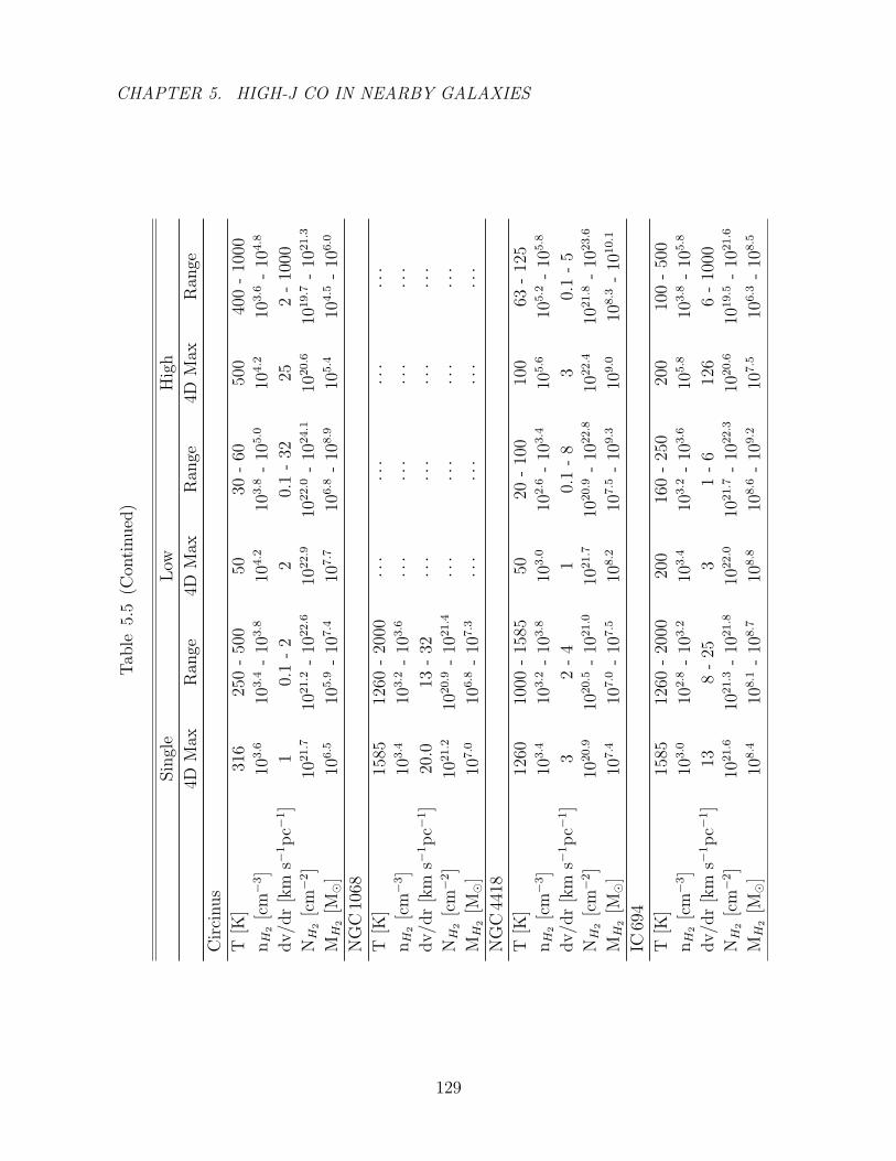
CHAPTER 5. HIGH-J CO IN NEARBY GALAXIES
Tab
le5.
5(C
onti
nued
)
Sin
gle
Low
Hig
h
4DM
axR
ange
4DM
axR
ange
4DM
axR
ange
Cir
cinus
T[K
]31
625
0-
500
5030
-60
500
400
-10
00
nH
2[c
m−
3]
103.6
103.4
-10
3.8
104.2
103.8
-10
5.0
104.2
103.6
-10
4.8
dv/d
r[k
ms−
1p
c−1]
10.
1-
22
0.1
-32
252
-10
00
NH
2[c
m−
2]
1021.7
1021.2
-10
22.6
1022.9
1022.0
-10
24.1
1020.6
1019.7
-10
21.3
MH
2[M
]10
6.5
105.9
-10
7.4
107.7
106.8
-10
8.9
105.4
104.5
-10
6.0
NG
C10
68
T[K
]15
8512
60-
2000
···
···
···
···
nH
2[c
m−
3]
103.4
103.2
-10
3.6
···
···
···
···
dv/d
r[k
ms−
1p
c−1]
20.0
13-
32···
···
···
···
NH
2[c
m−
2]
1021.2
1020.9
-10
21.4
···
···
···
···
MH
2[M
]10
7.0
106.8
-10
7.3
···
···
···
···
NG
C44
18
T[K
]12
6010
00-
1585
5020
-10
010
063
-12
5
nH
2[c
m−
3]
103.4
103.2
-10
3.8
103.0
102.6
-10
3.4
105.6
105.2
-10
5.8
dv/d
r[k
ms−
1p
c−1]
32
-4
10.
1-
83
0.1
-5
NH
2[c
m−
2]
1020.9
1020.5
-10
21.0
1021.7
1020.9
-10
22.8
1022.4
1021.8
-10
23.6
MH
2[M
]10
7.4
107.0
-10
7.5
108.2
107.5
-10
9.3
109.0
108.3
-10
10.1
IC69
4
T[K
]15
8512
60-
2000
200
160
-25
020
010
0-
500
nH
2[c
m−
3]
103.0
102.8
-10
3.2
103.4
103.2
-10
3.6
105.8
103.8
-10
5.8
dv/d
r[k
ms−
1p
c−1]
138
-25
31
-6
126
6-
1000
NH
2[c
m−
2]
1021.6
1021.3
-10
21.8
1022.0
1021.7
-10
22.3
1020.6
1019.5
-10
21.6
MH
2[M
]10
8.4
108.1
-10
8.7
108.8
108.6
-10
9.2
107.5
106.3
-10
8.5
129
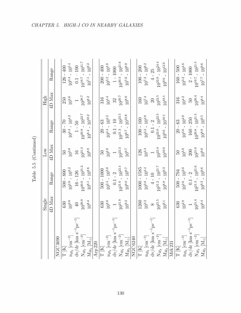
CHAPTER 5. HIGH-J CO IN NEARBY GALAXIES
Tab
le5.
5(C
onti
nued
)
Sin
gle
Low
Hig
h
4DM
axR
ange
4DM
axR
ange
4DM
axR
ange
NG
C36
90
T[K
]63
050
0-
800
5030
-70
250
126
-40
0
nH
2[c
m−
3]
103.0
102.8
-10
3.2
103.8
103.4
-10
4.2
103.6
103.4
-10
5.4
dv/d
r[k
ms−
1p
c−1]
4016
-12
616
1-
501
0.1
–10
0
NH
2[c
m−
2]
1020.9
1020.6
-10
21.2
1021.3
1020.9
-10
22.7
1020.7
1019.7
-10
21.7
MH
2[M
]10
8.4
108.1
-10
8.6
108.8
108.4
-10
10.2
108.2
107.1
-10
9.2
Arp
220
T[K
]63
050
0-
1000
5020
-63
316
200
-40
0
nH
2[c
m−
3]
102.8
102.4
-10
3.0
102.8
102.4
-10
3.2
104.4
103.2
-10
4.8
dv/d
r[k
ms−
1p
c−1]
10.
1-
21
0.1
-10
321
-10
00
NH
2[c
m−
2]
1021.9
1021.6
-10
22.4
1022.3
1021.3
-10
23.5
1020.7
1020.3
-10
21.6
MH
2[M
]10
9.2
109.0
-10
9.7
109.7
108.7
-10
10.8
108.0
107.6
-10
8.9
NG
C62
40
T[K
]12
6010
00-
1585
126
100
-16
016
010
0-
200
nH
2[c
m−
3]
103.2
103.0
-10
3.4
103.4
103.2
-10
3.8
107.4
107.2
-10
8.2
dv/d
r[k
ms−
1p
c−1]
84
-10
10.
1-
220
4-
25
NH
2[c
m−
2]
1021.5
1021.2
-10
21.7
1022.4
1022.0
-10
22.5
1022.5
1022.0
-10
24.4
MH
2[M
]10
9.1
108.8
-10
9.3
1010.0
109.6
-10
10.1
1010.1
109.6
-10
12.0
Mrk
231
T[K
]63
050
0-
794
5020
-63
316
160
-50
0
nH
2[c
m−
3]
102.8
102.6
-10
3.0
103.8
103.6
-10
4.0
104.2
103.2
-10
4.8
dv/d
r[k
ms−
1p
c−1]
10.
1-
220
016
0-
250
502
-10
00
NH
2[c
m−
2]
1021.4
1021.3
-10
21.6
1021.0
1020.8
-10
21.5
1020.4
1019.7
-10
21.5
MH
2[M
]10
9.4
109.3
-10
9.6
109.0
108.8
-10
9.5
108.4
107.7
-10
9.6
130
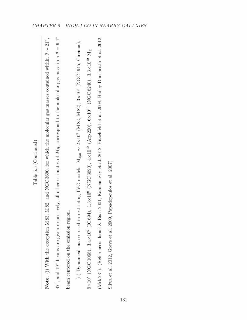
CHAPTER 5. HIGH-J CO IN NEARBY GALAXIES
Tab
le5.
5(C
onti
nued
)
Note.
(i)
Wit
hth
eex
cepti
onM
83,
M82
,an
dN
GC
3690
,fo
rw
hic
hth
em
olec
ula
rga
sm
asse
sco
nta
ined
wit
hinθ∼
21”,
47”,
and
19”
bea
ms
are
give
nre
spec
tive
ly,
all
other
esti
mat
esofM
H2
corr
esp
ond
toth
em
olec
ula
rga
sm
ass
inaθ
=9.
4”
bea
mce
nte
red
onth
eem
issi
onre
gion
.
(ii)
Dynam
ical
mas
ses
use
din
rest
rict
ing
LV
Gm
odel
s:Mdyn∼
2×10
9(M
83,
M82
),3×
109
(NG
C49
45,
Cir
cinus)
,
9×10
8(N
GC
1068
),3.
4×10
9(I
C69
4),
1.3×
109
(NG
C36
90),
4×10
10
(Arp
220)
,6×
1010
(NG
C62
40),
3.3×
1010
M
(Mrk
231)
.(R
efer
ence
s:Is
rael
&B
aas
2001
,K
amen
etzk
yet
al.
2012
,H
itsc
hfe
ldet
al.
2008
,H
aile
y-D
unsh
eath
etal
.20
12,
Sliw
aet
al.
2012
,G
reve
etal
.20
09,
Pap
adop
oulo
set
al.
2007
)
131
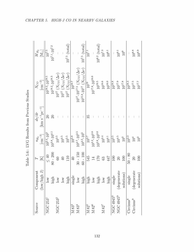
CHAPTER 5. HIGH-J CO IN NEARBY GALAXIES
Tab
le5.
6::
LV
GR
esult
sfr
omP
revio
us
Stu
die
s
Sou
rce
Com
pon
ent
TnH
2dv/d
rNCO
MH
2
(low
/hig
hJ)
[K]
[cm−
3]
[km
s−1p
c−1]
[cm−
2]
[M
]
NG
C25
31lo
w≤
4010
2.4
-103
2010
18.2
-101
8.5
107.5
hig
h80
-20
010
3.8
-104.1
2010
18.2
-101
8.3
107.1
-107.2
NG
C25
32lo
w60
103.5
–10
17
(NCO
/∆v)
–
low
4010
4.5
–10
17
(NCO
/∆v)
–
hig
h11
010
5.5
–10
17
(NCO
/∆v)
107.5
(tot
al)
M83
3si
ngl
e40
105.8
–10
18.7
–
M83
4lo
w30
-15
010
2.7
-103.5
–10
17-1
017.5
(NCO
/∆v)
–
hig
h60
-10
010
3.5
-105
–10
15.8
-101
7(N
CO
/∆v)
107.5
(tot
al)
M82
5hig
h54
510
3.7
3510
19
107.1
M82
6lo
w14
103.3
-103.8
–10
17.8
-101
8.0
–
hig
h17
010
2.8
-103.0
–10
19.5
108.2
(tot
al)
M82
7lo
w63
103.4
–10
18.6
107.3
hig
h44
710
4.1
–10
18.0
106.1
NG
C49
458
singl
e10
010
3.5
–10
18.8
–
NG
C49
459
(deg
ener
ate
2010
4.5
–10
17.9
109.1
solu
tion
s)10
010
3–
1017.8
109
Cir
cinus8
singl
e50
-80
103.3
–10
18.3
–
Cir
cinus9
(deg
ener
ate
2010
4–
1017.5
108.8
solu
tion
s)10
010
3–
1017.7
108.9
132
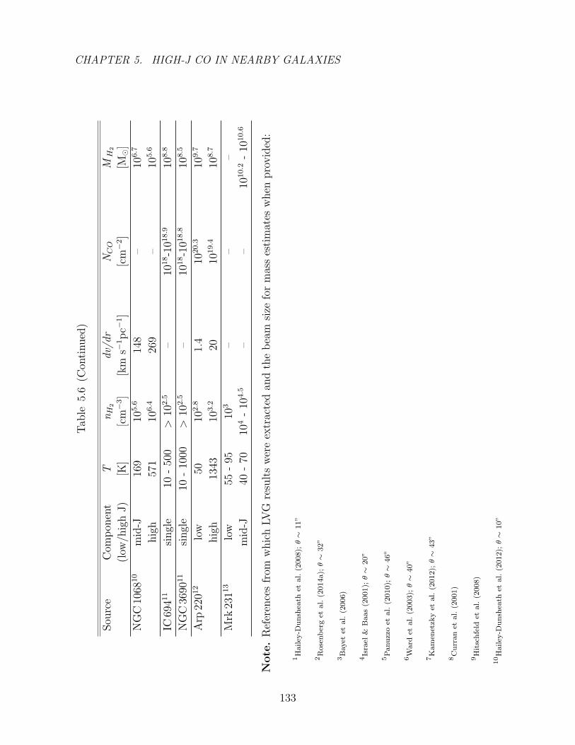
CHAPTER 5. HIGH-J CO IN NEARBY GALAXIES
Tab
le5.
6(C
onti
nued
)
Sou
rce
Com
pon
ent
TnH
2dv/d
rNCO
MH
2
(low
/hig
hJ)
[K]
[cm−
3]
[km
s−1p
c−1]
[cm−
2]
[M
]
NG
C10
6810
mid
-J16
910
5.6
148
–10
6.7
hig
h57
110
6.4
269
–10
5.6
IC69
411
singl
e10
-50
0>
102.5
–10
18-1
018.9
108.8
NG
C36
9011
singl
e10
-10
00>
102.5
–10
18-1
018.8
108.5
Arp
2201
2lo
w50
102.8
1.4
1020.3
109.7
hig
h13
4310
3.2
2010
19.4
108.7
Mrk
2311
3lo
w55
-95
103
––
–
mid
-J40
-70
104
-10
4.5
––
1010.2
-10
10.6
Note.
Ref
eren
ces
from
whic
hLV
Gre
sult
sw
ere
extr
acte
dan
dth
eb
eam
size
for
mas
ses
tim
ates
when
pro
vid
ed:
1H
ail
ey-D
un
shea
thet
al.
(2008);θ∼
11”
2R
ose
nb
erg
etal.
(2014a);θ∼
32”
3B
ayet
etal.
(2006)
4Is
rael
&B
aas
(2001);θ∼
20”
5P
anu
zzo
etal.
(2010);θ∼
46”
6W
ard
etal.
(2003);θ∼
40”
7K
am
enet
zky
etal.
(2012);θ∼
43”
8C
urr
an
etal.
(2001)
9H
itsc
hfe
ldet
al.
(2008)
10H
ail
ey-D
un
shea
thet
al.
(2012);θ∼
10”
133
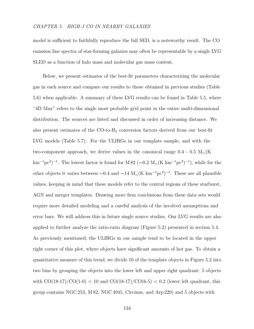
CHAPTER 5. HIGH-J CO IN NEARBY GALAXIES
model is sufficient to faithfully reproduce the full SED, is a noteworthy result. The CO
emission line spectra of star-forming galaxies may often be representable by a single LVG
SLED as a function of halo mass and molecular gas mass content.
Below, we present estimates of the best-fit parameters characterizing the molecular
gas in each source and compare our results to those obtained in previous studies (Table
5.6) when applicable. A summary of these LVG results can be found in Table 5.5, where
“4D Max” refers to the single most probable grid point in the entire multi-dimensional
distribution. The sources are listed and discussed in order of increasing distance. We
also present estimates of the CO-to-H2 conversion factors derived from our best-fit
LVG models (Table 5.7). For the ULIRGs in our template sample, and with the
two-component approach, we derive values in the canonical range 0.4 - 0.5 M(K
km−1pc2)−1. The lowest factor is found for M 82 (∼0.2 M(K km−1pc2)−1), while for the
other objects it varies between ∼0.4 and ∼14 M(K km−1pc2)−1. These are all plausible
values, keeping in mind that these models refer to the central regions of these starburst,
AGN and merger templates. Drawing more firm conclusions from these data sets would
require more detailed modeling and a careful analysis of the involved assumptions and
error bars. We will address this in future single source studies. Our LVG results are also
applied to further analyze the ratio-ratio diagram (Figure 5.2) presented in section 5.4.
As previously mentioned, the ULIRGs in our sample tend to be located in the upper
right corner of this plot, where objects have significant amounts of hot gas. To obtain a
quantitative measure of this trend, we divide 10 of the template objects in Figure 5.2 into
two bins by grouping the objects into the lower left and upper right quadrant: 5 objects
with CO(18-17)/CO(1-0) < 10 and CO(18-17)/CO(6-5) < 0.2 (lower left quadrant, this
group contains NGC 253, M 82, NGC 4945, Circinus, and Arp 220) and 5 objects with
134
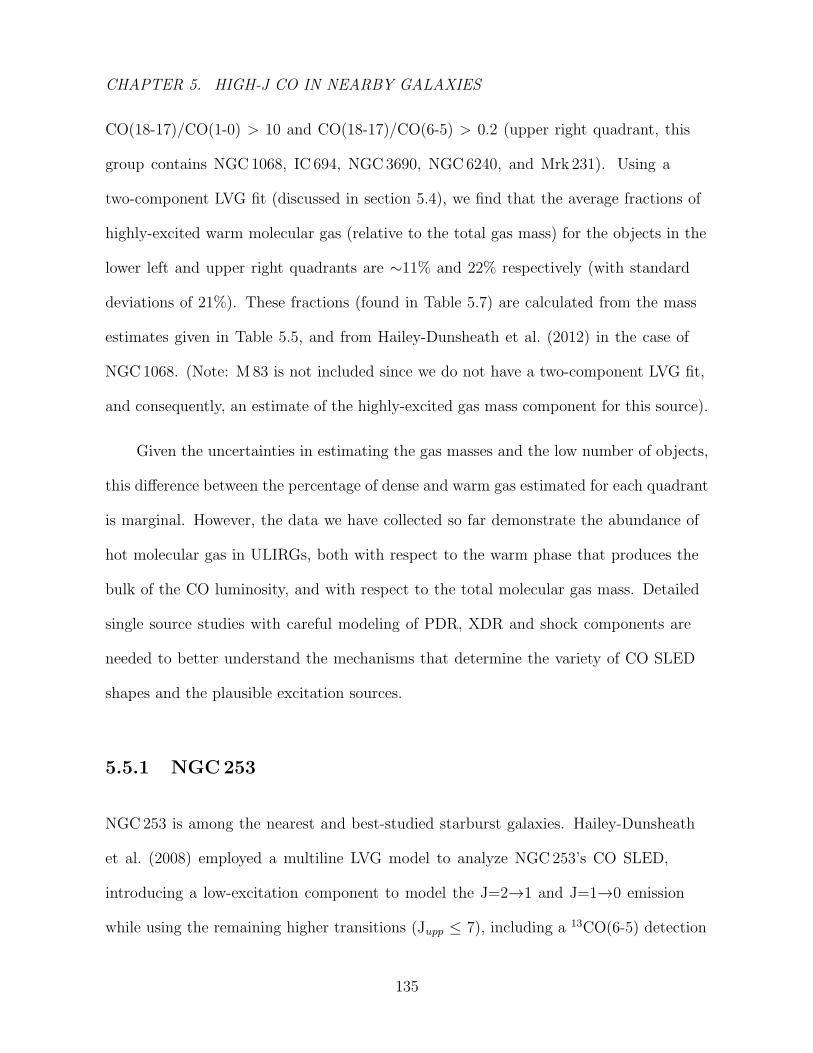
CHAPTER 5. HIGH-J CO IN NEARBY GALAXIES
CO(18-17)/CO(1-0) > 10 and CO(18-17)/CO(6-5) > 0.2 (upper right quadrant, this
group contains NGC 1068, IC 694, NGC 3690, NGC 6240, and Mrk 231). Using a
two-component LVG fit (discussed in section 5.4), we find that the average fractions of
highly-excited warm molecular gas (relative to the total gas mass) for the objects in the
lower left and upper right quadrants are ∼11% and 22% respectively (with standard
deviations of 21%). These fractions (found in Table 5.7) are calculated from the mass
estimates given in Table 5.5, and from Hailey-Dunsheath et al. (2012) in the case of
NGC 1068. (Note: M 83 is not included since we do not have a two-component LVG fit,
and consequently, an estimate of the highly-excited gas mass component for this source).
Given the uncertainties in estimating the gas masses and the low number of objects,
this difference between the percentage of dense and warm gas estimated for each quadrant
is marginal. However, the data we have collected so far demonstrate the abundance of
hot molecular gas in ULIRGs, both with respect to the warm phase that produces the
bulk of the CO luminosity, and with respect to the total molecular gas mass. Detailed
single source studies with careful modeling of PDR, XDR and shock components are
needed to better understand the mechanisms that determine the variety of CO SLED
shapes and the plausible excitation sources.
5.5.1 NGC253
NGC 253 is among the nearest and best-studied starburst galaxies. Hailey-Dunsheath
et al. (2008) employed a multiline LVG model to analyze NGC 253’s CO SLED,
introducing a low-excitation component to model the J=2→1 and J=1→0 emission
while using the remaining higher transitions (Jupp ≤ 7), including a 13CO(6-5) detection
135
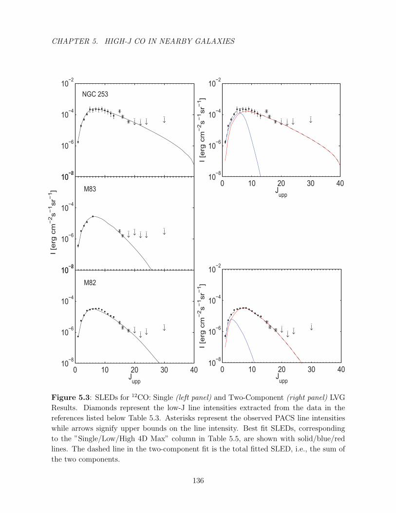
CHAPTER 5. HIGH-J CO IN NEARBY GALAXIES
10−8
10−6
10−4
10−2
↓ ↓ ↓↓
10−8
10−6
10−4
10−2
↓↓
↓ ↓↓
0 10 20 30 4010
−8
10−6
10−4
10−2
↓
↓↓
↓
I [e
rg c
m−
2s
−1sr−
1]
Jupp
0 10 20 30 4010
−8
10−6
10−4
10−2
↓
↓↓
↓
I [e
rg c
m−
2s
−1sr−
1]
Jupp
0 10 20 30 4010
−8
10−6
10−4
10−2
↓ ↓ ↓↓
I [e
rg c
m−
2s
−1sr−
1]
Jupp
NGC 253
M83
M82
Figure 5.3: SLEDs for 12CO: Single (left panel) and Two-Component (right panel) LVG
Results. Diamonds represent the low-J line intensities extracted from the data in the
references listed below Table 5.3. Asterisks represent the observed PACS line intensities
while arrows signify upper bounds on the line intensity. Best fit SLEDs, corresponding
to the ”Single/Low/High 4D Max” column in Table 5.5, are shown with solid/blue/red
lines. The dashed line in the two-component fit is the total fitted SLED, i.e., the sum of
the two components.
136
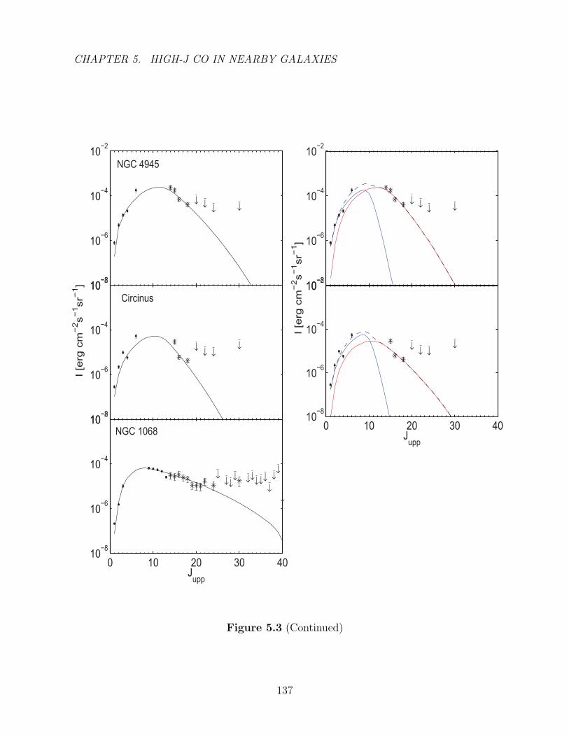
CHAPTER 5. HIGH-J CO IN NEARBY GALAXIES
10−8
10−6
10−4
10−2
↓↓
↓ ↓
10−8
10−6
10−4
10−2
↓↓ ↓
↓
0 10 20 30 4010
−8
10−6
10−4
10−2
↓
↓↓
↓ ↓↓
↓↓↓
↓
↓
↓
↓
I [e
rg c
m−
2s
−1sr−
1]
Jupp
0 10 20 30 4010
−8
10−6
10−4
10−2
↓↓ ↓
↓
I [e
rg c
m−
2s
−1sr−
1]
Jupp
10−8
10−6
10−4
10−2
↓↓
↓ ↓
NGC 4945
Circinus
NGC 1068
Figure 5.3 (Continued)
137
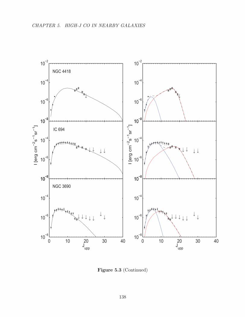
CHAPTER 5. HIGH-J CO IN NEARBY GALAXIES
10−8
10−6
10−4
10−2
↓
10−8
10−6
10−4
10−2
↓ ↓↓ ↓
10−8
10−6
10−4
10−2
↓ ↓↓ ↓
10−8
10−6
10−4
10−2
↓
0 10 20 30 4010
−8
10−6
10−4
10−2
↓ ↓ ↓↓ ↓
↓
↓
I [e
rg c
m−
2s
−1sr−
1]
Jupp
0 10 20 30 4010
−8
10−6
10−4
10−2
↓ ↓ ↓↓ ↓
↓
↓
I [e
rg c
m−
2s
−1sr−
1]
Jupp
NGC 4418
IC 694
NGC 3690
Figure 5.3 (Continued)
138
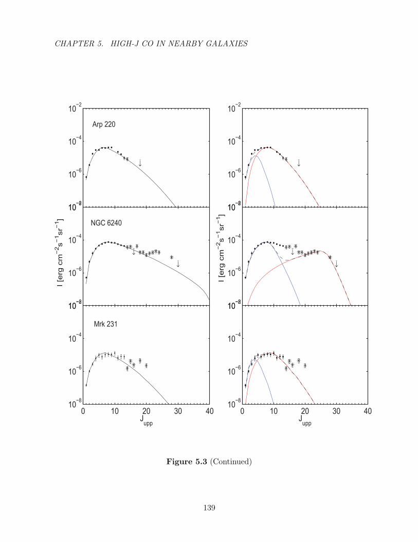
CHAPTER 5. HIGH-J CO IN NEARBY GALAXIES
10−8
10−6
10−4
10−2
↓
10−8
10−6
10−4
10−2
↓
↓
0 10 20 30 4010
−8
10−6
10−4
10−2
I [e
rg c
m−
2s
−1sr−
1]
Jupp
0 10 20 30 4010
−8
10−6
10−4
10−2
I [e
rg c
m−
2s
−1sr−
1]
Jupp
10−8
10−6
10−4
10−2
↓
↓
10−8
10−6
10−4
10−2
↓
Arp 220
NGC 6240
Mrk 231
Figure 5.3 (Continued)
139

CHAPTER 5. HIGH-J CO IN NEARBY GALAXIES
with ZEUS, to constrain the high-excitation component. Requiring that Tkin ≤ 200
K and restricting the velocity gradient to dv/dr ∼ 7 - 40 km s−1pc−1, they found a
low-excitation component characterized by Tkin ≤ 40 K and nH2 = 102.4 - 103.0 and a
high-excitation component with kinetic temperature in the range 80-200 K and nH2 =
103.8 - 104.1, with a velocity gradient of 20 km s−1pc−1 in both cases.
With the additional CO transition lines observed by SPIRE, Rosenberg et al.
(2014a) modeled the CO SLED as arising from three distinct molecular gas phases where
the low-J lines (Jupp < 5) originate from regions characterized by temperatures Tkin =
60 K and Tkin = 40 K, and number densities nH2 = 103.5 cm−3 and nH2 = 104.5 cm−3
respectively, while the mid-to-high-J lines (5 ≤ Jupp ≤ 13) are emitted by a region with
a kinetic temperature 110 K and number density of 105.5 cm−3.
In our analysis, we limit ourselves to two-phase molecular gas and model our
“high-excitation” component to fit the recent high-J line PACS observations (J=15→14,
16→15, and 18 →17), in addition to the mid-J lines. We find that the low and
high-excitation components are characterized by similar number densities, nH2 ∼ 103.4−3.6
cm−3, while the temperatures range from 50 K to 1260 K for each respective component.
We estimate a total H2 mass of ∼ 5×10⁷ M, only ∼2% of which is in the warm phase
generating the high-J CO line emission.
5.5.2 M83
For the nearby, barred starburst galaxy M 83, Israel & Baas (2001) presented two LVG
models to fit the Jupper ≤ 4 CO emission lines: one with Tkin = 30-150 K and nH2 =
102.7-103.5 cm−3, and one with Tkin = 60-100 K and nH2 = 103.5-105.0 cm−3. Bayet et al.
140
CHAPTER 5. HIGH-J CO IN NEARBY GALAXIES
(2006), modeling the Jupper ≤ 6 CO emission lines as originating from a single region,
suggested a fit with Tkin = 40 K and nH2 = 105.8 cm−3.
With only two high-J line measurements for this source, CO(15-14) and CO(16-15),
we do not fit a two-component model in this case due to the underdetermined nature
of the problem. However, we find that the observed CO SLED for M 83 is reasonably
well-fitted by a single-component model with a kinetic temperature of ∼ 500 K and a H2
number density of 102.8 cm−3. The molecular mass traced by the CO emission within the
central 325 pc of the source (θ ∼ 21”) in this best-fit model is 1.3×10⁷ M, close to the
total gas mass estimate of 3×10⁷ M derived in Israel & Baas (2001).
5.5.3 M82
Due to its proximity, M 82 is an extensively studied starburst galaxy. Panuzzo et al.
(2010) fit the 12CO emission spectrum from J=4→3 to J=13→12 using a LVG model
with Tkin = 545 K, nH2 = 103.7 cm−3, and dv/dr = 35 km s−1pc−1. Kamenetzky et al.
(2012) proposed a two-component model where the cool molecular gas (traced by those
lines below J=4→3) was characterized by a kinetic temperature of 63 K and a H2 number
density of 103.4 cm−3, while the high-J CO lines traced a very warm gas component with
Tkin = 447 K and nH2 = 104.1 cm−3.
With the inclusion of the additional constraints on the high-excitation component
provided by the PACS lines CO(15-14), CO(16-15), and CO(18-17), we find that
our fitted parameters compare very well with the two-component model set forth in
Kamenetzky et al. (2012). Our LVG analysis yields a warm component with Tkin = 500
K and nH2 = 103.4 cm−3, and a cool component characterized by a kinetic temperature
141

CHAPTER 5. HIGH-J CO IN NEARBY GALAXIES
of 80 K, a H2 number density of 103.2 cm−3, and a velocity gradient of ∼ 200 km s−1pc−1.
This high velocity gradient in the low-excitation component is suspected to be the culprit
behind the low CO-to-H2 conversion factor in M 82, αCO ∼ 0.25 M/(K km−1pc2). Since
the optical depth of the J = 1→0 line is reduced by a large dv/dr, less molecular mass
is required to produce the observed flux, leading to a reduced estimate of MH2,tot and
consequently, of αCO. The total H2 mass within the 47”×47” PACS beam is estimated to
be ∼ 5×10⁷ M, of the same order as the mass estimates derived in Ward et al. (2003),
Panuzzo et al. (2010), and Kamenetzky et al. (2012), with 50% of the mass in the warm
component.
5.5.4 NGC4945 & Circinus
At distances of ∼ 3.7 and ∼ 4 Mpc, NGC 4945 and Circinus are among the nearest
and most infrared-bright spiral galaxies in the sky, with observations of their obscured
nuclei classifying them as Seyfert galaxies. In both NGC 4945 and Circinus, Hitschfeld
et al. (2008) used the ratios of the observed integrated intensities of the 12CO(1-0) to
12CO(4-3) lines, as well as the 13CO(1-0) and 13CO(2-1) transitions to obtain column
densities, H2 number densities, and kinetic temperatures for the two sources. Fitting
the CO and 13CO lines, they found a degeneracy in the best-fit parameters in nH2-Tkin
plane. Their best fit solution for NGC 4945 was nH2 = 3×104 cm−3 and Tkin = 20 K, a
solution not significantly better than one with nH2 = 103 cm−3 and Tkin = 100 K. Curran
et al. (2001) found a solution with nH2 = 3×103 cm−3 and Tkin = 100 K from 12CO
observations of the three lowest transitions and 13CO data of the two lowest transitions.
For Circinus, again, Hitschfeld et al. (2008) found a number of solutions that
142
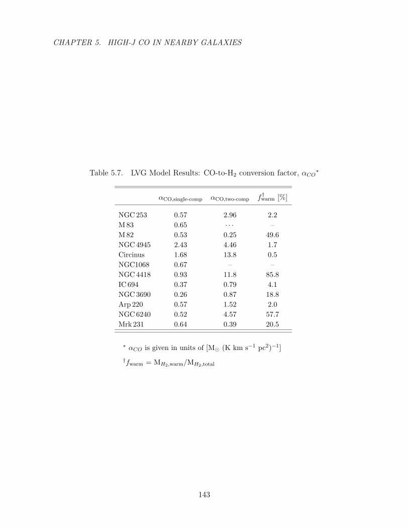
CHAPTER 5. HIGH-J CO IN NEARBY GALAXIES
Table 5.7. LVG Model Results: CO-to-H2 conversion factor, αCO∗
αCO,single-comp αCO,two-comp f †warm [%]
NGC 253 0.57 2.96 2.2
M 83 0.65 · · · –
M 82 0.53 0.25 49.6
NGC 4945 2.43 4.46 1.7
Circinus 1.68 13.8 0.5
NGC1068 0.67 – –
NGC 4418 0.93 11.8 85.8
IC 694 0.37 0.79 4.1
NGC 3690 0.26 0.87 18.8
Arp 220 0.57 1.52 2.0
NGC 6240 0.52 4.57 57.7
Mrk 231 0.64 0.39 20.5
∗ αCO is given in units of [M (K km s−1 pc2)−1]
†fwarm = MH2,warm/MH2,total
143
CHAPTER 5. HIGH-J CO IN NEARBY GALAXIES
provided consistent CO cooling curves for the low-J transitions. The lowest χ2 was
obtained for nH2 = 104 cm−3 and Tkin = 20 K; a second, degenerate, solution was found
with nH2 = 103 cm−3 and Tkin = 100 K. Their results agreed well with Curran et al.
(2001), who found a best-fit solution with Tkin = 50-80 K and nH2 = 2×103 cm−3 from
observations of the three lowest 12CO transitions and the two lowest 13 CO transitions in
this source.
Our LVG analysis of the 12CO(1-0) to 12CO(6-5) lines yields low-excitation
components with parameters consistent with those obtained by Hitschfeld et al. (2008).
We find best-fit solutions with a kinetic temperature of 50 K for both sources, and an
H2 number density of 104.8 cm−3 and 104.2 cm−3 in NGC 4945 and Circinus, respectively.
Modeling the high-J CO emission lines as originating from a separate region leads to
a warmer, denser component characterized by Tkin = 316 K and nH2 = 105 cm−3 in
NGC 4945, and Tkin = 500 K and nH2 = 104.2 cm−3 in Circinus. We estimate a total H2
gas mass of 4 - 5×10⁷ M in both sources, of which only ∼ 0.5 - 1% is in the warm phase.
5.5.5 NGC1068
NGC 1068 is one of the brightest and best studied Seyfert 2 galaxies. Its CO SLED,
including the PACS high-J lines, has been extensively analyzed by us (Hailey-Dunsheath
et al. 2012) and in the works of Spinoglio et al. (2012); we direct the reader to those
papers and to Table 5.5 for a summary of the LVG-modeled gas excitation in this source.
We only note that our single-component model yields an H2 gas mass of 107 M, twice
the total gas mass estimated by Hailey-Dunsheath et al. (2012).
144
CHAPTER 5. HIGH-J CO IN NEARBY GALAXIES
5.5.6 NGC4418
NGC 4418 is a peculiar, single nucleus galaxy, with a LIRG-like luminosity (≈ 1011L)
but with other properties similar to warm ULIRGs, like a high LFIR/MH2 ratio,
an extreme [C II] deficit (e.g.Gracia-Carpio et al. 2011), and an extremely compact
luminosity source (Evans et al. 2003).
We find that a cool gas phase characterized by Tkin = 50 K and nH2 = 1000 cm−3
gives rise to the three lowest 12CO transitions, while the corresponding high-J lines are
emitted by a denser, warmer component with Tkin = 100 K and nH2 = 105.6 cm−3. The
gas mass is estimated to be ∼108 and 109 M in each of the respective components,
indicating that a significant portion of the molecular gas (∼85%) is in a dense, warm
phase.
5.5.7 IC 694 & NGC3690
The two galaxies IC 694 and NGC 3690 form the luminous infrared merger system
known as Arp 299. The nuclear region of IC 694 shows the typical mid-IR characteristics
of ULIRGs (very compact and dust-enshrouded star formation, probably harboring a
low-luminosity AGN), while the nuclear region of NGC 3690 hosts a Seyfert 2 AGN and
is surrounded by regions of star formation.
Strong 12CO emission has been detected in the nuclei of both IC 694 and NGC 3690.
Sliwa et al. (2012) modeled the ratios of the observed integrated intensities of the
13CO(2-1) transition and the low-J 12CO lines in these two sources. Their best-fit LVG
solutions for IC 694 and NGC 3690 had kinetic temperatures ranging from 10 to 500 K
145
CHAPTER 5. HIGH-J CO IN NEARBY GALAXIES
and 10 to 1000 K, respectively, and a H2 number density greater than 102.5 cm−3 in both
cases.
For IC 694, we find that the low and high-J lines can be modeled as arising from two
distinct components characterized by the same kinetic temperature, 200 K, but different
H2 number densities, 103.4 cm−3 and 105.8 cm−3, where the high-J emission originates
from the denser component. The molecular gas mass in each of these components is
estimated to be ∼ 7×10⁸ and 3×10⁷ M, respectively. The total gas mass estimate
is consistent with the gas mass estimates of the molecular region modeled after the
low-J lines in Sliwa et al. (2012), as well as the mass estimates derived in Rosenberg
et al. (2014b) using only PDR heating. However, as evident from the LVG-modeled CO
SLED for this source (Figure 5.3), this two-component best-fit model under-predicts the
observed mid-J lines (9 ≤ Jupp ≤ 14), suggesting that in the case of IC 694, at least three
distinct components are necessary in fitting the full CO SLED.
The observed CO SLED for NGC 3690 (including the extended emission region
where its’ galaxy disk overlaps with that of IC 694), is well-fit by a two-component LVG
model in which the low-J lines arise from a cool gas phase (Tkin = 50 K) while the high-J
line emission originates from a warmer gas phase (Tkin = 250 K). These two components,
which both contribute to the mid-J line emission, are characterized by similar number
densities (4-6×103 cm−3) and have a combined gas mass of nearly 109 M.
5.5.8 Arp 220
At a distance of about 77 Mpc, Arp 220 is one of the nearest and best studied
ULIRGs, serving as a template for high-z studies of dusty starbursts. We found that
146

CHAPTER 5. HIGH-J CO IN NEARBY GALAXIES
a single-component model with Tkin = 630 K and nH2 = 102.8 cm−3 reproduces the
observed CO SLED quite well, yielding an associated H2 gas mass of ∼ 109 M.
Rangwala et al. (2011) found that the low-J transitions trace cold gas with Tkin
= 50 K and nH2 = 102.8 cm−3, while the mid-J to high-J lines trace a warmer, denser
component with Tkin = 1350 K and nH2 = 103.2 cm−3, yielding a total gas mass of
∼ 6×10⁹ M. Our two-component LVG analysis yields identical results for the cool
molecular gas region; however, we find that the mid to high-J lines are modeled best
as arising from a high-excitation component with Tkin = 316 K and nH2 = 104.4 cm−3.
The difference in these values when compared against the best-fit parameters obtained
in Rangwala et al. (2011) for the high-excitation component may be due to the fact
that the high-J CO lines are differentially affected by dust extinction, an effect which
Rangwala et al. (2011) argues and accounts for in his modeling, but which was not taken
into account in this analysis. Nonetheless, our two-component LVG model yields a total
gas mass MH2 ∼ 6×10⁹ M, (of which only 2% is in the warm phase), consistent with
the mass estimates derived in Rangwala et al. (2011).
5.5.9 NGC6240
NGC 6240 is a nearby luminous infrared galaxy, with a CO SLED similar in shape to
that of Mrk 231. Several X-ray studies have firmly established the presence of powerful
AGN activity (e.g. Iwasawa & Comastri 1998; Vignati et al. 1999), in fact occurring
in both nuclei (Komossa et al. 2003). The system is also known for strong shocked
emission in the superwind flow that is driven by the NGC 6240 starburst (van der Werf
et al. 1993; Lutz et al. 2003). Although the CO J=8→7 transition has the largest line
147
CHAPTER 5. HIGH-J CO IN NEARBY GALAXIES
intensity, the Jupper ≥ 14 transitions make a significant contribution, with the intensity
of the individual CO lines only slowly decreasing for higher rotational quantum numbers.
Limiting ourselves to a two-component LVG analysis, we find that the low-J lines
can be modeled as arising from a region with Tkin = 126 K and nH2 = 103.4 cm−3, while
the high-J lines are produced by a slightly warmer (Tkin = 160 K) and much denser
gas phase, with a H2 number density of 107.4 cm−3. The total gas mass derived for this
simplistic model is 2×10¹⁰ M, with close to 60% of the gas in the warmer, denser phase.
However, as in the case of IC 694, this two-component LVG model fails to reproduce
the observed mid-J lines, suggesting that three distinct components may be necessary
to fit the full CO SLED. An alternative approach may be to employ shock models to
further analyze the CO excitation in NGC 6240. This was pointed out in Meijerink et al.
(2013) when they found, among other things, that even the most optimistic estimate of
the AGN X-ray luminosity is not enough to explain the combined H2 and CO observed
luminosities.
5.5.10 Mrk 231
Mrk 231 is the most luminous of the local ULIRGs and a type 1, low-ionization broad
absorption line (LoBAL) AGN. Limited to observations of the CO ladder up to the
J=6→5 transition in Mrk 231, Papadopoulos et al. (2007) found that while the LVG
solutions derived solely from the three lowest CO transitions converged to Tkin = 55 -95
K and nH2 ∼ 103 cm−3, the CO(4-3) and CO(6-5) emission lines traced a much denser
gas phase with nH2 ∼ (1-3)×104 cm−3.
With the additional SPIRE FTS (van der Werf et al. 2010) and PACS high-J lines,
148

CHAPTER 5. HIGH-J CO IN NEARBY GALAXIES
we find that the CO lines up to J = 11-10 can be produced by a two-component LVG
model, with a cool region at Tkin = 50 K and nH2 = 103.8 cm−3 emitting the low-J
lines (Jupper < 4) and a warmer, denser region at Tkin = 316 K and nH2 = 104.2 cm−3
dominating the mid- to high-J line emissions. These models yield a total associated gas
mass of ∼ 109 M, with 20% of the gas in the high-excitation component. However, a
challenge is presented by the highest CO rotational lines (Jupper ≥ 12), which are strongly
under-produced by our two-component LVG model. These higher-J lines may signal the
presence of a third excitation component which could be a high-excitation PDR, XDR,
or shocks, as explained in van der Werf et al. (2010).
5.6 Summary
We have presented the extragalactic detections of FIR CO rotational line emission within
the central 10” of a sample of starburst galaxies, Seyfert galaxies, and (U)LIRGs in the
local universe. (z < 0.1). We have augmented our multi-J 12CO line dataset (Jupp ≥ 14),
detected with Herschel-PACS, with lower-J CO line measurements collected from the
literature to yield a well-sampled set of local CO SLEDs (Tables 5.3 and 5.4). Along
with providing a necessary benchmark for the usually more sparsely sampled SLEDs
obtained for high redshift galaxies, (e.g. Weiss et al. 2007), these SLEDs demonstrate
the uncertainties in relying solely on high-J CO diagnostics to characterize the excitation
source of a galaxy. Without a broad coverage of the entire SLED for a given source, a
single or few observed CO lines can easily be misinterpreted given the sheer diversity
in SLED shapes shown in Figure 5.1. However, while the detection of a high-J CO line
alone is not an unambiguous signature of a particular excitation source, the position
149
CHAPTER 5. HIGH-J CO IN NEARBY GALAXIES
of a source on a ratio-ratio diagram may be an indication of the presence, or lack
thereof, of a warm, dense molecular gas component. In the CO(18-17)/CO(1-0) versus
CO(18-17)/CO(6-5) plot shown in Figure 5.2, the sources that fall in the upper right
corner of the diagram, with CO(18-17)/CO(1-0) > 10 and CO(18-17)/CO(6-5) > 0.2,
consistently have a higher percentage of highly-excited molecular gas than those that fall
in the lower left corner, as verified by the LVG-modeling results for these sources.
Another tracer of high density molecular clouds, which is traditionally used in
ground-based mm observations, is provided by low HCN lines. These lines trace
similar critical densities as the CO lines in the PACS range (n ∼ 106 - 108 cm−3). In
fact, a similar trend is found if in the above ratio-ratio plot the x-axis is replaced by
the HCN(1-0)/CO(1-0) ratios of our objects as presented in Gao & Solomon (2004).
However, while both molecules trace dense gas, the energy levels of the upper transitions
are different, i.e. the CO traces warmer gas than HCN, and therefore, while HCN lines
provide complementary results, they are not 1:1 substitutes for the high-J CO lines.
Furthermore, at high redshifts, the CO lines have moved into the (sub-)mm range and
are thus better high density tracers than the low-lying HCN transitions which have
moved out of that window.
These results were verified using an LVG radiative transfer modeling technique,
which we employed to quantitatively analyze the CO emission from a subset of our
detected sources. For each CO SLED, we identify the set of characterizing parameters
that best reproduces the observed line intensities. Using both single-component and
two-component LVG models to fit the cloud’s kinetic temperature, velocity gradient, gas
density, and beam-averaged CO column density, we derive the molecular gas mass and
the corresponding CO-to-H2 conversion factor for each respective source. A summary of
150

CHAPTER 5. HIGH-J CO IN NEARBY GALAXIES
the best-fit LVG parameters is presented in Table 5.5 and the resulting LVG-modeled
SLEDs for the single and two-component fits are shown in the left and right panels
of Figure 5.3, respectively. Remarkably, the CO emission line spectra of star-forming
galaxies may often be representable by a single LVG SLED as a function of halo mass
and molecular gas mass content. Furthermore, we find that our two-component LVG
model results are mostly consistent with the fits obtained in Kamenetzky et al. (2014)
where the 12CO SLEDs from J=1→0 to J=13→12 are modeled for many of the same
sources discussed in this paper.
Estimates of the CO-to-H2 conversion factors derived from our best-fit single and
two-component LVG models can be found in Table 5.7. The relatively low αCO values
we find (compared to normal, star-forming galaxies like the Milky Way), are consistent
with previous measures of the conversion factor for some of the individual sources as
well as the general finding of low αCO’s in the center of bright galaxies (Wild et al. 1992;
Bryant & Scoville 1996; Scoville et al. 1997; Bryant & Scoville 1999; Papadopoulos &
Seaquist 1999; Israel 2009b,a; Sliwa et al. 2012). Conditions such as low metallicity, high
gas temperature, large velocity dispersion, and higher gas density in an extended warm
phase outside the GMCs (typical in ULIRGs) all drive αCO to lower values (Bolatto et al.
2013). While the high velocity gradient is the primary culprit behind the reduced value
of αCO in M 82 (∼ 0.25 M(K km−1pc2)−1), the bulk of our results are due to the higher
temperatures and warm-phase gas densities found in our sample targets (which never
approach the low-metallicity regime.) However, given our modest sample size and the
small degree of variance we find in the warm gas mass fractions, it becomes difficult to
identify any specific trend between these physical conditions and the conversion factor.
We also systematically find higher αCO values for the two-component models which
151
CHAPTER 5. HIGH-J CO IN NEARBY GALAXIES
provide separate fits for the low-and high-J lines, than for the single component models
where all CO line emissions trace a single region. This trend is consistent with the
existence of a dichotomy, most prominent in (U)LIRGS, pointed out in Papadopoulos
et al. (2012b). In their analysis of a CO line survey of (U)LIRGs, Papadopoulos et al.
(2012b) find that while one-phase radiative transfer models of the global CO SLEDs
yield low αCO values, < αCO >∼ 0.6 M(K km−1pc2)−1, in cases where higher-J CO
lines allow a separate assessment of gas mass at high densities, near-Galactic αCO ∼
(3-6) M(K km−1pc2)−1 values become possible.
In addition to the CO lines presented here, each of the objects of this study also has
(SHINING and other) observations of the FIR fine-structure lines. These will provide
further constraints on the physical properties of the photon-dominated regions (PDRs),
X-ray dominated regions (XDRs), and shocks in these galaxies, and will augment the
interpretation of the CO emission in future detailed studies.
5.7 Acknowledgements
N.M. is supported by the Raymond and Beverly Sackler Tel Aviv University-Harvard
Astronomy Program. We thank the DFG for support via German-Israeli Project
Cooperation grant STE1869/1-1.GE625/15-1. Basic research in IR astronomy at NRL
is funded by the US ONR; J.F. also acknowledges support from the NHSC. E.G-A
is a Research Associate at the Harvard-Smithsonian Center for Astrophysics. AV
thanks the Leverhulme Trust for a Research Fellowship. S.V. also acknowledges partial
support from NASA through Herschel grants 1427277 and 1454738. PACS has been
developed by a consortium of institutes led by MPE (Germany) and including UVIE
152
CHAPTER 5. HIGH-J CO IN NEARBY GALAXIES
(Austria); KU Leuven, CSL, IMEC (Belgium); CEA, LAM (France); MPIA (Germany);
INAF-IFSI/OAA/OAP/OAT, LENS, SISSA (Italy); IAC (Spain). This development has
been supported by the funding agencies BMVIT (Austria), ESA-PRODEX (Belgium),
CEA/CNES (France), DLR (Germany), ASI/INAF (Italy), and CICYT/MCYT (Spain).
This material is based upon work supported by the National Science Foundation
Graduate Research Fellowship under Grant No. DGE1144152. Any opinion, findings,
and conclusions or recommendations expressed in this material are those of the authors
and do not necessarily reflect the views of the National Science Foundation.
153
Chapter 6
Predicting the Intensity Mapping
Signal for multi-J CO lines
This thesis chapter originally appeared in the literature as
N. Mashian, A. Sternberg, and A. Loeb, Predicting the
intensity mapping signal for multi-J CO lines, Journal of
Cosmology and Astroparticle Physics, 11, 028, 2015
6.1 Abstract
We present a novel approach to estimating the intensity mapping signal of any CO
rotational line emitted during the Epoch of Reionization (EoR). Our approach is based
on large velocity gradient (LVG) modeling, a radiative transfer modeling technique
that generates the full CO spectral line energy distribution (SLED) for a specified gas
kinetic temperature, volume density, velocity gradient, molecular abundance, and column
154
CHAPTER 6. INTENSITY MAPPING SIGNAL FOR CO LINES
density. These parameters, which drive the physics of CO transitions and ultimately
dictate the shape and amplitude of the CO SLED, can be linked to the global properties
of the host galaxy, mainly the star formation rate (SFR) and the SFR surface density.
By further employing an empirically derived SFR−M relation for high redshift galaxies,
we can express the LVG parameters, and thus the specific intensity of any CO rotational
transition, as functions of the host halo mass M and redshift z. Integrating over the
range of halo masses expected to host CO-luminous galaxies, we predict a mean CO(1-0)
brightness temperature ranging from ∼ 0.6 µK at z = 6 to ∼ 0.03 µK at z = 10 with
brightness temperature fluctuations of ∆2CO ∼ 0.1 and 0.005 µK respectively, at k =
0.1 Mpc−1. In this model, the CO emission signal remains strong for higher rotational
levels at z = 6, with 〈TCO〉 ∼ 0.3 and 0.05 µK for the CO J = 6→5 and CO J = 10→9
transitions respectively. Including the effects of CO photodissociation in these molecular
clouds, especially at low metallicities, results in the overall reduction in the amplitude
of the CO signal, with the low- and high-J lines weakening by 2-20% and 10-45%,
respectively, over the redshift range 4 < z < 10.
6.2 Introduction
Within the last decade, spectral line intensity mapping has been proposed as an
additional, complementary probe of the large-scale structure (LSS) of star-forming
galaxies during the epoch of reionization (EoR) (Suginohara et al. 1999; Righi et al.
2008; Visbal & Loeb 2010). Glimpses into this era have been limited to observations of
individual massive galaxies and quasars at high redshifts, provided by the Hubble Space
Telescope (HST) and ground-based telescopes. While in the future, we anticipate new
155

CHAPTER 6. INTENSITY MAPPING SIGNAL FOR CO LINES
instruments like Atacama Large Millimeter Array (ALMA) and the James Webb Space
Telescope (JWST) providing more detailed views of this “cosmic dawn”, they will be
restricted by relatively small fields of view and an inability to observe galaxies that are
simply too faint to detect individually. Intensity mapping offers a complementary glimpse
of the three-dimensional structure of the high-redshift universe by imaging aggregate line
emissions from thousands of unresolved objects and studying the large-scale fluctuations
in the given line intensity due to the clustering of unresolved sources.
Intensity mapping can be performed using many different spectral lines, the 21
cm neutral hydrogen line being among the most common, given its unique insight
into the evolution of the neutral IGM during the EoR (Madau et al. 1997; Loeb &
Zaldarriaga 2004; Zaldarriaga et al. 2004; Furlanetto et al. 2006; Morales & Wyithe
2010; Pritchard & Loeb 2011). In this paper, we focus on the millimeter to far-infrared
rotational transitions of carbon monoxide (CO), a molecule that forms primarily in
star-forming regions and whose intensity maps promise a wealth of information on the
spatial distribution of star formation in the universe (Breysse et al. 2014). While CO
intensity fluctuations have already been studied, initially as foreground contaminants
to cosmic microwave background (CMB) measurements (Righi et al. 2008) and then as
probes of LSS (Visbal & Loeb 2010; Carilli 2011; Gong et al. 2011; Lidz et al. 2011;
Pullen et al. 2013), these studies have been limited to the lowest order transitions of the
molecule, mainly, CO(1-0) and CO(2-1). These lines are often considered because they
are typically among the brightest and have redshifted frequencies that can potentially
be observed from the ground. However, with the advent of ALMA1 and its frequency
1http://almascience.nrao.edu
156
CHAPTER 6. INTENSITY MAPPING SIGNAL FOR CO LINES
coverage (84 - 950 GHz), fluctuations in the line emission of many high-J CO transitions
will potentially be available and can be measured and translated into a 3D map of
the early universe. Having access to multiple CO rotational lines will further facilitate
redshift identification and mitigate line confusion, making it possible to statistically
isolate the fluctuations from a particular redshift by cross-correlating the emission from
different sets of lines (Visbal & Loeb 2010; Loeb & Furlanetto 2013).
Attempts in the recent literature to obtain a theoretical estimate of the CO emission
signal from high redshift galaxies have relied heavily on empirical relations calibrated
from local observations and are limited almost exclusively to the 12CO J=1→0 transition
line. To calculate this mean CO brightness, a simple model is often adopted that connects
the strength of the CO emission to the abundance of the dark matter halos that host CO
luminous galaxies. Visbal & Loeb (2010) construct this model by first approximating
a galaxy’s star formation rate (SFR) as a linear function of the mass of the galaxy’s
host halo. They then further assume a linear relationship between the line luminosity
and SFR and adopt the LCO to SFR ratio from M 82 to calibrate the proportionality
constant. Lidz et al. (2011) embrace a similar approach, adopting the SFR −M
relation proposed by Visbal & Loeb (2010), but using a set of empirical scaling relations
between a galaxy’s SFR, far-infrared luminosity, and CO(1-0) luminosity that have been
measured for galaxies at z . 3. Both studies lead to a simple empirical estimate of the
CO luminosity that is linear in halo mass (LCO ∝ SFR ∝ M) and that relies on the
extrapolation of low-redshift calibrations to higher redshifts, redshifts corresponding to
the EoR. Gong et al. (2011) arrives at the relation between CO(1-0) luminosity and
the halo mass via a different route, making use of the Millennium numerical simulation
results of Obreschkow et al. (2009), a study which, although incorporates many physical
157
CHAPTER 6. INTENSITY MAPPING SIGNAL FOR CO LINES
processes to model the CO emission from high-redshift galaxies, still invokes low-redshift
measurements to calibrate the normalization factor of the CO luminosity for a given
halo.
These various models, among others, have led to estimates of the CO power spectra
amplitude signal that vary over a range spanning two orders of magnitude, illustrating
the lack of theoretical understanding of the physics of CO transitions in a high-redshift
context (Breysse et al. 2014). In Munoz & Furlanetto (2013), this problem is addressed
and a computation of CO fluxes is presented within an analytic framework that
incorporates both global modes of star formation and the physics of molecular rotational
lines in z & 6 Lyman-break galaxies. Our paper follows the general direction taken by
Munoz & Furlanetto (2013) and introduces a simpler approach that captures and ties the
physics of molecular emission lines to high-redshift (z ≥ 4) observations of star-forming
galaxies (Mashian et al. 2016). Our approach is based on large velocity gradient (LVG)
modeling, a radiative transfer modeling technique that generates the full CO spectral
line energy distribution (SLED) for a specified set of physical parameters. Typically,
LVG modeling is employed to quantitatively analyze an observed set of emission lines
and determine the set of parameters that best reproduce the observed SED (Mashian
et al. 2015b). In this paper, we consider applying the LVG methodology in the reverse
direction: given a halo of mass M with CO-emitting molecular clouds characterized by
a kinetic temperature Tkin, velocity gradient dv/dr, gas volume density n, molecular
abundance χ, and column density N , we will derive the full CO SED and compute the
mean surface brightness of any CO rotational line emitted by halos with that mass at
any given redshift.
Our paper is organized as follows. In section 6.3, we introduce our LVG model
158

CHAPTER 6. INTENSITY MAPPING SIGNAL FOR CO LINES
for the specific intensity of CO emission and outline the formalism that relates the set
of LVG parameters driving the physics of CO transitions in molecular clouds to the
global properties of the host galaxy, mainly, the SFR. Given the empirically determined
high-redshift SFR −M relation (Mashian et al. 2016), these parameters, and thus, the
specific CO intensity, can ultimately be expressed as functions of the host halo mass M
and redshift z. In section 6.4 we compute the spatially averaged CO surface brightness
from star-forming galaxies, as well as the power spectrum of spatial fluctuations in the
CO emission at any given redshift, with a focus on redshifts corresponding to the EoR.
We conclude in section 6.5 with a summary of our results and a brief comparison with
other related calculations of the CO intensity mapping signal. Throughout we consider a
ΛCDM cosmology parametrized by ns = 1, σ8 = 0.8, δc = 1.69, Ωm = 0.31, ΩΛ = 0.69,
Ωb = 0.05, and h = 0.7, consistent with the latest measurements from Planck (Planck
Collaboration et al. 2016b).
6.3 Modeling the CO Emission
6.3.1 CO Brightness Temperature
To calculate the average CO brightness temperature, we follow the formalism presented
by Lidz et al. (2011) and consider the specific intensity of a CO line observed at frequency
νobs at redshift z = 0,
I(νobs) =c
4π
∫ ∞0
dz′ε [νobs(1 + z′)]
H(z′)(1 + z′)4(6.1)
as determined by solving the cosmological radiative transfer equation, where H(z) is the
Hubble parameter and ε [νobs(1 + z′)] is the proper volume emissivity of the given line.
159
CHAPTER 6. INTENSITY MAPPING SIGNAL FOR CO LINES
Since CO is emitted from within halos hosting star-forming galaxies, we take the CO
luminosity, LCO, to be some function of the halo mass M and redshift, and assume the
profile of each CO line is a delta function in frequency,
LCO = L(M, z)δD(ν − νJ) (6.2)
where νJ is the rest frame frequency of the transition of interest. If we then further
assume that at any given time, a fraction fduty of halos with mass larger than Mmin,CO
actively emit CO lines, then for a given halo mass function dn/dM , the volume emissivity
is,
ε(ν, z) = δD(ν − νJ)(1 + z)3fduty
∫ ∞Mmin,CO
dMdn
dM(M, z)L(M, z) (6.3)
The specific intensity of a line with rest frame frequency νJ , emitted by gas at
redshift zJ thus simplifies to
Iνobs =c
4π
1
νJH(zJ)fduty
∫ ∞Mmin,CO
dMdn
dM(M, zJ)L(M, zJ) (6.4)
or, written as the brightness temperature,
〈TCO〉 =c3
8π
(1 + zJ)2
kBν3JH(zJ)
fduty
∫ ∞Mmin,CO
dMdn
dM(M, zJ)L(M, zJ) (6.5)
where kB is the Boltzmann constant.
To determine L(M, zJ), the specific luminosity of a given CO line, we employ large
velocity gradient (LVG) modeling, a method of radiative transfer in which the excitation
and opacity of CO lines are determined by the kinetic temperature Tkin, velocity gradient
dv/dr, gas density n, CO-to-H2 abundance ratio χCO, and the CO column density of the
emitting source. We adopt the escape probability formalism (Castor 1970; Goldreich &
Kwan 1974) derived for a spherical cloud undergoing uniform collapse where
βJ =1− eτJτJ
(6.6)
160
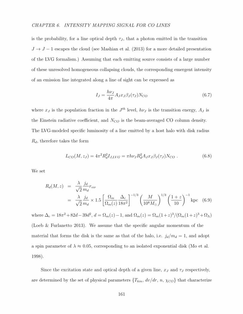
CHAPTER 6. INTENSITY MAPPING SIGNAL FOR CO LINES
is the probability, for a line optical depth τJ , that a photon emitted in the transition
J → J − 1 escapes the cloud (see Mashian et al. (2013) for a more detailed presentation
of the LVG formalism.) Assuming that each emitting source consists of a large number
of these unresolved homogeneous collapsing clouds, the corresponding emergent intensity
of an emission line integrated along a line of sight can be expressed as
IJ =hνJ4π
AJxJβJ(τJ)NCO (6.7)
where xJ is the population fraction in the J th level, hνJ is the transition energy, AJ is
the Einstein radiative coefficient, and NCO is the beam-averaged CO column density.
The LVG-modeled specific luminosity of a line emitted by a host halo with disk radius
Rd, therefore takes the form
LCO(M, zJ) = 4π2R2dIJ,LV G = πhνJR
2dAJxJβJ(τJ)NCO . (6.8)
We set
Rd(M, z) =λ√2
jdmd
rvir
=λ√2
jdmd
× 1.5
[Ωm
Ωm(z)
∆c
18π2
]−1/3(M
108M
)1/3(1 + z
10
)−1
kpc (6.9)
where ∆c = 18π2 +82d−39d2, d = Ωm(z)−1, and Ωm(z) = Ωm(1+z)3/(Ωm(1+z)3 +ΩΛ)
(Loeb & Furlanetto 2013). We assume that the specific angular momentum of the
material that forms the disk is the same as that of the halo, i.e. jd/md = 1, and adopt
a spin parameter of λ ≈ 0.05, corresponding to an isolated exponential disk (Mo et al.
1998).
Since the excitation state and optical depth of a given line, xJ and τJ respectively,
are determined by the set of physical parameters Tkin, dv/dr, n, χCO that characterize
161
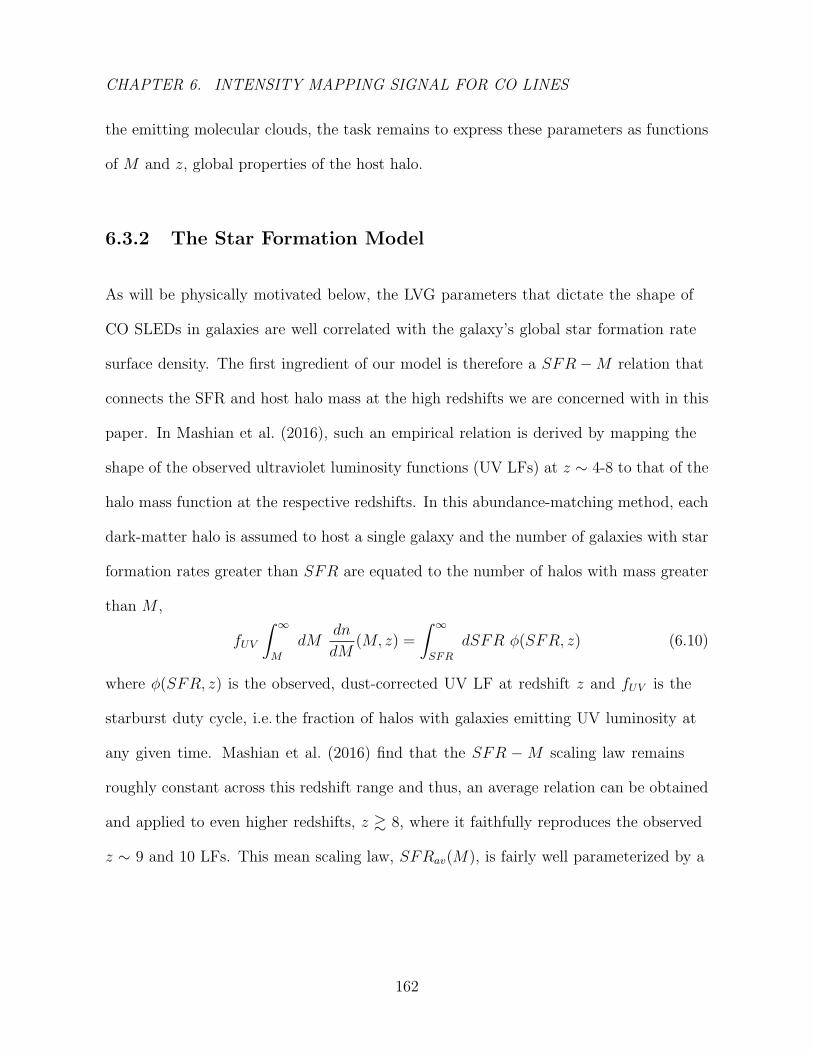
CHAPTER 6. INTENSITY MAPPING SIGNAL FOR CO LINES
the emitting molecular clouds, the task remains to express these parameters as functions
of M and z, global properties of the host halo.
6.3.2 The Star Formation Model
As will be physically motivated below, the LVG parameters that dictate the shape of
CO SLEDs in galaxies are well correlated with the galaxy’s global star formation rate
surface density. The first ingredient of our model is therefore a SFR −M relation that
connects the SFR and host halo mass at the high redshifts we are concerned with in this
paper. In Mashian et al. (2016), such an empirical relation is derived by mapping the
shape of the observed ultraviolet luminosity functions (UV LFs) at z ∼ 4-8 to that of the
halo mass function at the respective redshifts. In this abundance-matching method, each
dark-matter halo is assumed to host a single galaxy and the number of galaxies with star
formation rates greater than SFR are equated to the number of halos with mass greater
than M ,
fUV
∫ ∞M
dMdn
dM(M, z) =
∫ ∞SFR
dSFR φ(SFR, z) (6.10)
where φ(SFR, z) is the observed, dust-corrected UV LF at redshift z and fUV is the
starburst duty cycle, i.e. the fraction of halos with galaxies emitting UV luminosity at
any given time. Mashian et al. (2016) find that the SFR −M scaling law remains
roughly constant across this redshift range and thus, an average relation can be obtained
and applied to even higher redshifts, z & 8, where it faithfully reproduces the observed
z ∼ 9 and 10 LFs. This mean scaling law, SFRav(M), is fairly well parameterized by a
162
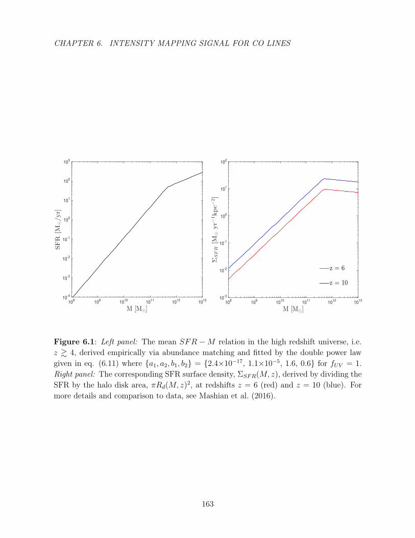
CHAPTER 6. INTENSITY MAPPING SIGNAL FOR CO LINES
M [M⊙]10
810
910
1010
1110
1210
13
SFR
[M⊙/yr]
10-4
10-3
10-2
10-1
100
101
102
103
M [M⊙]10
810
910
1010
1110
1210
13
ΣSFR[M
⊙yr−
1kpc−
2]
10-3
10-2
10-1
100
101
102
z = 6
z = 10
Figure 6.1: Left panel: The mean SFR −M relation in the high redshift universe, i.e.
z & 4, derived empirically via abundance matching and fitted by the double power law
given in eq. (6.11) where a1, a2, b1, b2 = 2.4×10⁻¹⁷, 1.1×10⁻⁵, 1.6, 0.6 for fUV = 1.
Right panel: The corresponding SFR surface density, ΣSFR(M, z), derived by dividing the
SFR by the halo disk area, πRd(M, z)2, at redshifts z = 6 (red) and z = 10 (blue). For
more details and comparison to data, see Mashian et al. (2016).
163
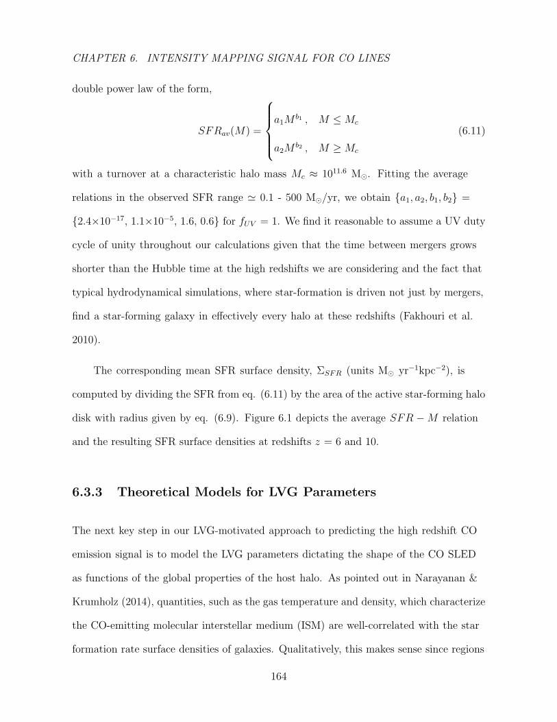
CHAPTER 6. INTENSITY MAPPING SIGNAL FOR CO LINES
double power law of the form,
SFRav(M) =
a1M
b1 , M ≤Mc
a2Mb2 , M ≥Mc
(6.11)
with a turnover at a characteristic halo mass Mc ≈ 1011.6 M. Fitting the average
relations in the observed SFR range ' 0.1 - 500 M/yr, we obtain a1, a2, b1, b2 =
2.4×10⁻¹⁷, 1.1×10⁻⁵, 1.6, 0.6 for fUV = 1. We find it reasonable to assume a UV duty
cycle of unity throughout our calculations given that the time between mergers grows
shorter than the Hubble time at the high redshifts we are considering and the fact that
typical hydrodynamical simulations, where star-formation is driven not just by mergers,
find a star-forming galaxy in effectively every halo at these redshifts (Fakhouri et al.
2010).
The corresponding mean SFR surface density, ΣSFR (units M yr−1kpc−2), is
computed by dividing the SFR from eq. (6.11) by the area of the active star-forming halo
disk with radius given by eq. (6.9). Figure 6.1 depicts the average SFR −M relation
and the resulting SFR surface densities at redshifts z = 6 and 10.
6.3.3 Theoretical Models for LVG Parameters
The next key step in our LVG-motivated approach to predicting the high redshift CO
emission signal is to model the LVG parameters dictating the shape of the CO SLED
as functions of the global properties of the host halo. As pointed out in Narayanan &
Krumholz (2014), quantities, such as the gas temperature and density, which characterize
the CO-emitting molecular interstellar medium (ISM) are well-correlated with the star
formation rate surface densities of galaxies. Qualitatively, this makes sense since regions
164

CHAPTER 6. INTENSITY MAPPING SIGNAL FOR CO LINES
of high SFR density typically arise from denser gas concentrations and have large UV
radiation fields, with increased efficiency for thermal coupling between gas and dust.
In the following sections, we will outline how each LVG parameter can be expressed in
terms of the SFR surface density, ΣSFR, and thus ultimately as a function of just the
halo mass and redshift.
6.3.3.1 Gas Kinetic Temperature
To determine the effective kinetic temperature of the CO-emitting molecular gas, we
assume that the gas and dust in the star-forming disk are thermally well-coupled, i.e.
Tgas ≈ Tdust. The temperature of a dust grain is set by the balance of radiative heating
and cooling processes taking place in molecular clouds. The rate of heating due to
absorption of optical or UV radiation and the incident cosmic microwave background
(CMB) can be written as(dE
dt
)abs
= πa2
[∫ ∞0
dν Qabs,UV (ν)Fν(ν) + σSBT4CMB
](6.12)
where σSB is the Stefan-Boltzmann constant, a is the grain radius, Qabs,UV (ν) is the
emissivity in the UV-optical regime, which we set equal to unity (Chanial et al. 2007),
TCMB = 2.73(1+z) is the CMB temperature and Fν(ν) is the flux of energy radiated
by the central starburst in the disk. Assuming optically thick conditions requires this
starlight energy to be totally reemitted in the infrared; the integral on the right-hand
side can thus be expressed as LIR/4πR2d and, adopting the conversion between LIR and
SFR presented in Kennicutt (1998b),(LIR
erg s−1
)= 2.2× 1043
(SFR
M yr−1
), (6.13)
165
CHAPTER 6. INTENSITY MAPPING SIGNAL FOR CO LINES
eq. (6.12) takes the final form:(dE
dt
)abs
= πa2
[2.2× 1043
4π
ΣSFR
(M yr−1kpc−2)+ σSB(2.73(1 + z))4
]. (6.14)
The rate of cooling of dust grains by infrared emission is given by(dE
dt
)em
= 4πa2
∫ ∞0
dν Qabs,IR(ν)πBν(ν, Td) (6.15)
where Qabs,IR(ν) ' Qabs(ν0)(ν/ν0)β is the emissivity in the infrared regime, ν0 is the
reference frequency, and β is the dust emissivity index. Substituting in for Qabs,IR(ν)
and πBν(ν, Td) (the flux emitted by a black-body), the integral simplifies to(dE
dt
)em
= πa2
[60σSBπ4
(kBh
)βQabs(ν0)
νβ0Γ(β + 4)ζ(β + 4)T β+4
d
]. (6.16)
At thermal equilibrium, (dE/dt)abs = (dE/dt)em, and the steady-state grain
temperature in units of kelvin is
Td(ΣSFR(M, z), z) =
(π4
60
(h
kB
)βνβ0
Qabs(ν0)
1
Γ(β + 4)ζ(β + 4)
[2.3× 10⁻³
4πσSB
ΣSFR(M, z)
(M yr−1kpc−2)
+(2.73(1 + z))4])1/(β+4)
. (6.17)
In the analysis below, we take the fiducial value of β = 1.3, consistent with the mean
emissivity index derived from the SCUBA Local Universe Galaxy Survey (Dunne et al.
2000), and the standard value Qabs(125 µm) = 7.5×10⁻⁴ (Hildebrand 1983; Alton et al.
2004; Chanial et al. 2007). A plot of the kinetic temperature as a function of halo mass
at different redshifts can be found in the left panel of Figure 6.2.
6.3.3.2 Cloud volume density
Another key parameter in determining the shape of the CO SLED is n, the cloud volume
density (cm−3) of the dominant collision partner for CO rotational excitation. Since we
166

CHAPTER 6. INTENSITY MAPPING SIGNAL FOR CO LINES
M [M⊙]10
810
910
1010
1110
1210
13
Tkin[K
]
60
65
70
75
80
85
90
95
100
M [M⊙]10
810
910
1010
1110
1210
13
nH
2[cm
−3]
101
102
103
104
105
106
z = 6
z = 10
Figure 6.2: Left panel: Gas kinetic temperature assuming the fiducial values β = 1.3 and
Qabs(125 µm) = 7.5×10⁻⁴ in eq. (6.17). Right panel: Cloud volume density of molecular
hydrogen as defined by eqs. (6.18)-(6.27) plotted at redshifts z = 6 (red) and z = 10
(blue).
167
CHAPTER 6. INTENSITY MAPPING SIGNAL FOR CO LINES
are assuming CO-emitting molecular clouds, n in this case is the cloud volume density of
H2, given by
nH2 =3Σcl
4µmH2rcl(6.18)
where µ = 1.36 takes into account the helium contribution to the molecular weight
(assuming cold, neutral gas), mH2 = 3.34×10⁻²⁷ kg, and rcl is the cloud radius assuming
a uniform sphere. At these high redshifts where the ISM is dominated by molecular
gas, the surface density of H2 in a given molecular cloud, Σcl, can be related to the
beam-averaged gas surface density in the galactic disk, Σgas.
Empirical studies have found that a correlation exists between the surface density
of molecular gas and the surface density of the SFR, a discovery that is consistent with
observations that stars form predominantly in the molecular component of the ISM.
The Kennicutt-Schmidt (KS) relation (Schmidt 1959; Kennicutt 1989) formulates this
correlation in terms of a power-law, 〈ΣSFR〉 ∝ 〈Σgas〉N , where estimates of the index
N range from super-linear (Kennicutt 1989, 1998b; Bouche et al. 2007; Liu et al. 2011;
Momose et al. 2013), to linear (Bigiel et al. 2008; Leroy et al. 2008, 2013), to sublinear
(Shetty et al. 2014). Given our paper’s focus on high redshift star-forming sources with
CO-emitting molecular clouds, we deemed it most appropriate to adopt the KS relation
presented in Genzel et al. (2010),
ΣSFR = (3.3± 0.6)× 10−4
(Σgas
1 M pc−2
)1.2±0.1
M yr−1 kpc−2 , (6.19)
a relation that was derived from data sets of CO molecular emission in z ∼ 1-3 normal
star-forming galaxies and restricted to the regime where molecular gas dominates the ISM
at these redshifts, i.e. Σgas & 3 M pc−2. Since no evidence of any redshift-dependence
of this relation has been found thus far, applying eq. (6.19) at the higher redshifts we
168
CHAPTER 6. INTENSITY MAPPING SIGNAL FOR CO LINES
consider in this paper, z ≥ 4, is a reasonable extrapolation.
We therefore set Σcl equal to Σgas, as defined by eq. (6.19), except in cases where
Σgas drops below the threshold surface density for which the cloud is predominantly
molecular. This “star-formation” threshold, defined by a molecular gas fraction of fH2 =
0.5, is derived in Sternberg et al. (2014) for a plane-parallel slab (including H2 dust) as a
function of metallicity Z ′,
Σgas,∗(Z′) =
2m
σg(Z ′)
(1.6 ln
[αG(Z ′)
3.2+ 1
])(6.20)
where m = 2.34×10⁻²⁷ kg is the mean particle mass per hydrogen nucleus,
σg(Z′) = 1.9 × 10⁻²¹Z ′ cm−2 is the dust-grain Lyman-Werner-photon absorption cross
section per hydrogen nucleon, and αG is the dimensionless parameter that defines the
LW-band optical depth in the cloud due to HI dust,
αG(Z ′) =
(1 + 3.1Z
′0.365
4.1
)6.78
1 +√
2.64Z ′. (6.21)
We adopt the fundamental metallicity relation (FMR), a tight relation between the
gas-phase metallicity Z ′, stellar mass M∗, and SFR, to ultimately express Z ′ as a function
solely of the halo mass and redshift. The FMR was initially observed and formulated
in Mannucci et al. (2010) for local galaxies in the mass range 9.2 ≤ logM∗/M ≤ 11.4.
Since then, the FMR has been confirmed to hold for star-forming galaxies at redshifts
as high as z ∼ 3 Belli et al. (2013), and to extend smoothly at lower masses (Mannucci
et al. 2011), taking the final form,
12 + log (O/H) =
8.90 + 0.37m− 0.14s− 0.19m2 + 0.12ms− 0.054s2 for µ0.32 ≥ 9.5
8.93 + 0.51(µ0.32 − 10) for µ0.32 < 9.5
(6.22)
169
CHAPTER 6. INTENSITY MAPPING SIGNAL FOR CO LINES
where µα = log (M∗)− α log (SFR), m = log (M∗)− 10, and s = log (SFR).
To further parametrize the metallicity as a function of the halo mass and redshift,
we rely on observations and models that support the conclusion that the SFR in galaxies
at redshifts z & 4 scales nearly linearly with increasing stellar mass and does not vary
by more than a factor of order 2 (Salmon et al. 2015). This behavior is consistent with a
crude estimation of the stellar mass of a galaxy with a star formation rate SFR:
M∗ ∼∫ tH(z)
0
dt SFR(t) ∼ SFR(z)× tH(z) (6.23)
where tH(z) is the age of the universe at a given redshift z. Since each halo of interest
formed at some fraction of the age of the universe, the right-hand side should be
multiplied by a factor . 1. We therefore calibrate the above expression using the
SFR-M∗ best-fit parameters presented in Salmon et al. (2015) for z ∼ 4 - 6 and obtain
the following relation
M∗(M, z) = (0.28± 0.02)SFRav(M) tH(z) (6.24)
where SFRav(M) is the average SFR for a halo of mass M . We assume this relation
continues to apply at redshifts z > 6 in the following calculations.
Armed with the parametrization of SFR introduced in section 6.3.2, and thus a
metallicity Z expressed solely as a function of halo mass and redshift, we can now return
to our model for the cloud surface density, Σcl. To ensure the molecular state of each
individual cloud, i.e. fH2 ≥ 0.5, we set Σcl equal to the beam-averaged gas surface
density Σgas(M, z) (derived by inverting eq. (6.19)) for all halo masses M > M and floor
170
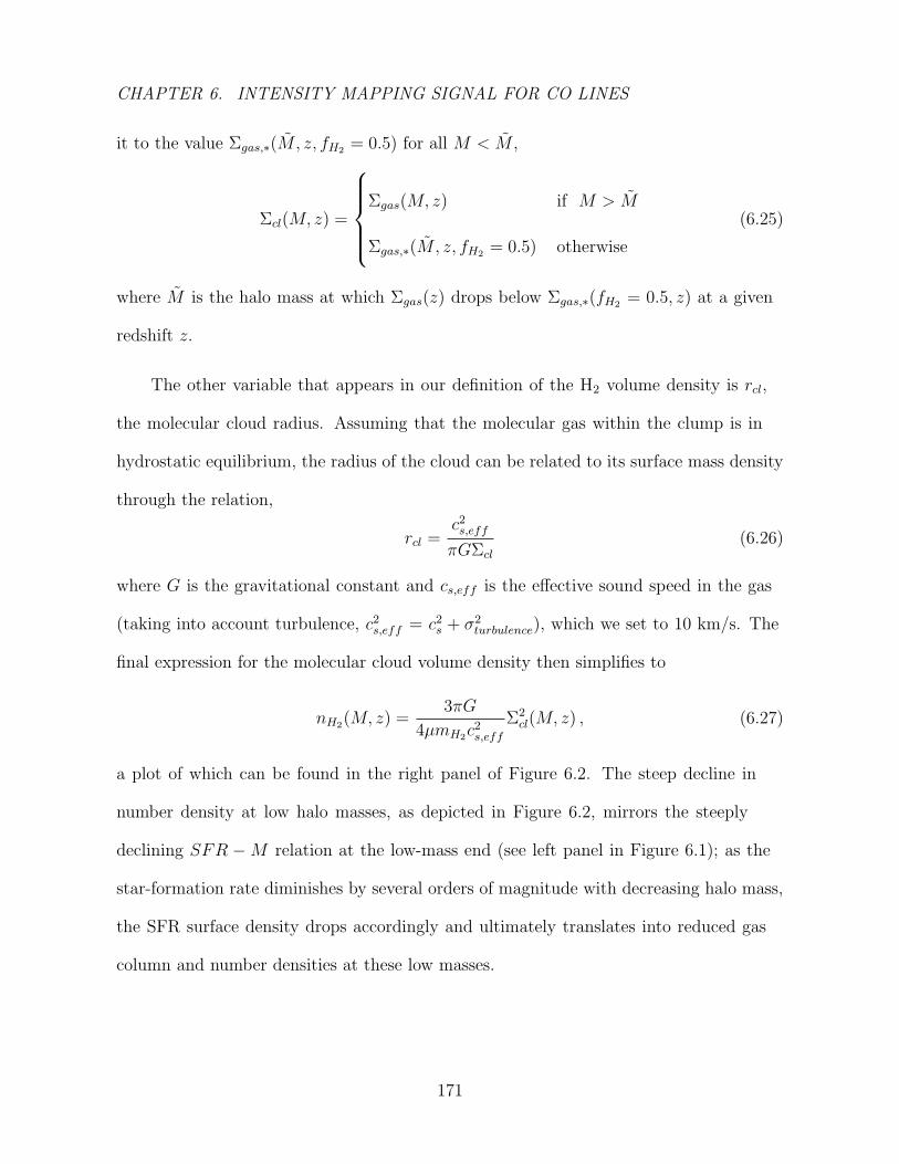
CHAPTER 6. INTENSITY MAPPING SIGNAL FOR CO LINES
it to the value Σgas,∗(M, z, fH2 = 0.5) for all M < M ,
Σcl(M, z) =
Σgas(M, z) if M > M
Σgas,∗(M, z, fH2 = 0.5) otherwise
(6.25)
where M is the halo mass at which Σgas(z) drops below Σgas,∗(fH2 = 0.5, z) at a given
redshift z.
The other variable that appears in our definition of the H2 volume density is rcl,
the molecular cloud radius. Assuming that the molecular gas within the clump is in
hydrostatic equilibrium, the radius of the cloud can be related to its surface mass density
through the relation,
rcl =c2s,eff
πGΣcl
(6.26)
where G is the gravitational constant and cs,eff is the effective sound speed in the gas
(taking into account turbulence, c2s,eff = c2
s + σ2turbulence), which we set to 10 km/s. The
final expression for the molecular cloud volume density then simplifies to
nH2(M, z) =3πG
4µmH2c2s,eff
Σ2cl(M, z) , (6.27)
a plot of which can be found in the right panel of Figure 6.2. The steep decline in
number density at low halo masses, as depicted in Figure 6.2, mirrors the steeply
declining SFR −M relation at the low-mass end (see left panel in Figure 6.1); as the
star-formation rate diminishes by several orders of magnitude with decreasing halo mass,
the SFR surface density drops accordingly and ultimately translates into reduced gas
column and number densities at these low masses.
171
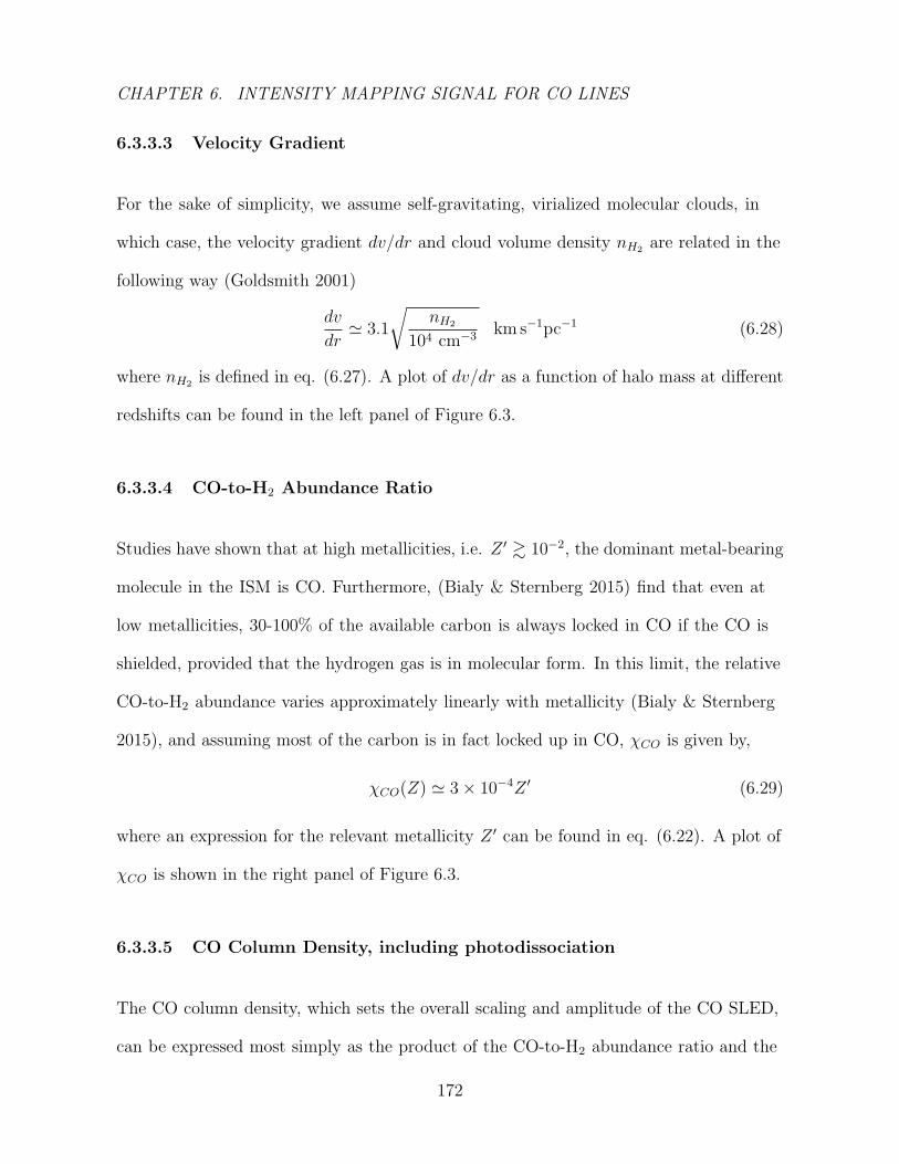
CHAPTER 6. INTENSITY MAPPING SIGNAL FOR CO LINES
6.3.3.3 Velocity Gradient
For the sake of simplicity, we assume self-gravitating, virialized molecular clouds, in
which case, the velocity gradient dv/dr and cloud volume density nH2 are related in the
following way (Goldsmith 2001)
dv
dr' 3.1
√nH2
104 cm−3 km s−1pc−1 (6.28)
where nH2 is defined in eq. (6.27). A plot of dv/dr as a function of halo mass at different
redshifts can be found in the left panel of Figure 6.3.
6.3.3.4 CO-to-H2 Abundance Ratio
Studies have shown that at high metallicities, i.e. Z ′ & 10−2, the dominant metal-bearing
molecule in the ISM is CO. Furthermore, (Bialy & Sternberg 2015) find that even at
low metallicities, 30-100% of the available carbon is always locked in CO if the CO is
shielded, provided that the hydrogen gas is in molecular form. In this limit, the relative
CO-to-H2 abundance varies approximately linearly with metallicity (Bialy & Sternberg
2015), and assuming most of the carbon is in fact locked up in CO, χCO is given by,
χCO(Z) ' 3× 10⁻⁴Z ′ (6.29)
where an expression for the relevant metallicity Z ′ can be found in eq. (6.22). A plot of
χCO is shown in the right panel of Figure 6.3.
6.3.3.5 CO Column Density, including photodissociation
The CO column density, which sets the overall scaling and amplitude of the CO SLED,
can be expressed most simply as the product of the CO-to-H2 abundance ratio and the
172
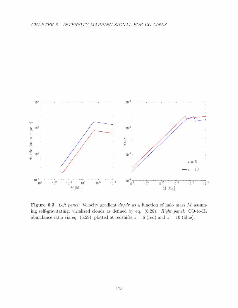
CHAPTER 6. INTENSITY MAPPING SIGNAL FOR CO LINES
M [M⊙]10
810
910
1010
1110
1210
13
dv/dr[km
s−1pc−1]
10-1
100
101
102
M [M⊙]10
810
910
1010
1110
1210
13
χCO
10-6
10-5
10-4
10-3
z = 6
z = 10
Figure 6.3: Left panel: Velocity gradient dv/dr as a function of halo mass M assum-
ing self-gravitating, virialized clouds as defined by eq. (6.28). Right panel: CO-to-H2
abundance ratio via eq. (6.29), plotted at redshifts z = 6 (red) and z = 10 (blue).
173
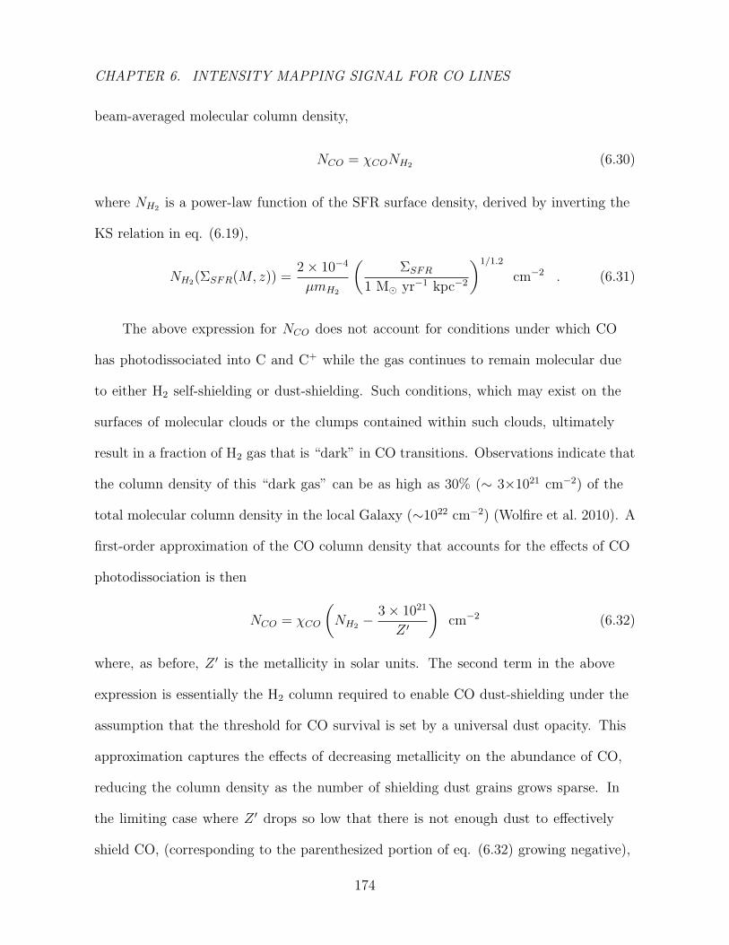
CHAPTER 6. INTENSITY MAPPING SIGNAL FOR CO LINES
beam-averaged molecular column density,
NCO = χCONH2 (6.30)
where NH2 is a power-law function of the SFR surface density, derived by inverting the
KS relation in eq. (6.19),
NH2(ΣSFR(M, z)) =2× 10⁻⁴
µmH2
(ΣSFR
1 M yr−1 kpc−2
)1/1.2
cm−2 . (6.31)
The above expression for NCO does not account for conditions under which CO
has photodissociated into C and C+ while the gas continues to remain molecular due
to either H2 self-shielding or dust-shielding. Such conditions, which may exist on the
surfaces of molecular clouds or the clumps contained within such clouds, ultimately
result in a fraction of H2 gas that is “dark” in CO transitions. Observations indicate that
the column density of this “dark gas” can be as high as 30% (∼ 3×1021 cm−2) of the
total molecular column density in the local Galaxy (∼1022 cm−2) (Wolfire et al. 2010). A
first-order approximation of the CO column density that accounts for the effects of CO
photodissociation is then
NCO = χCO
(NH2 −
3× 10²¹
Z ′
)cm−2 (6.32)
where, as before, Z ′ is the metallicity in solar units. The second term in the above
expression is essentially the H2 column required to enable CO dust-shielding under the
assumption that the threshold for CO survival is set by a universal dust opacity. This
approximation captures the effects of decreasing metallicity on the abundance of CO,
reducing the column density as the number of shielding dust grains grows sparse. In
the limiting case where Z ′ drops so low that there is not enough dust to effectively
shield CO, (corresponding to the parenthesized portion of eq. (6.32) growing negative),
174

CHAPTER 6. INTENSITY MAPPING SIGNAL FOR CO LINES
M [M⊙]10
810
910
1010
1110
1210
13
NCO[cm
−2]
1015
1016
1017
1018
1019
1020
1021
Photodissociation OFF, eq. (2.30)Photodissociation ON, eq. (2.32)
z = 6
z = 10
Figure 6.4: Beam-averaged CO column density derived at redshifts z=6 (red) and z=10
(blue) under conditions where CO photodissociation is accounted for (solid curves, eq.
(6.32)) and neglected (dashed curves, eq. (6.31)). In the case where the effects of CO
photodissociation are included, the CO column density drops to zero for halos smaller
than M . 1010 M, indicating that the CO in the gas has fully disassociated.
175
CHAPTER 6. INTENSITY MAPPING SIGNAL FOR CO LINES
the CO is fully dissociated and NCO is set to zero. We note that eq. (6.32) is only a
first-order approximation and that the constant, 3×10²¹, can be altered due to variations
in UV field intensity or gas clumping factors. The beam-averaged CO column density at
different redshifts is plotted in Figure 6.4, both for the case where CO photodissociation
is accounted for (solid curves) and neglected (dashed curves).
6.3.4 Model CO SLEDs
Equipped with analytic expressions for the LVG parameters that dictate the shape and
magnitude of the CO SLED, we can now compute the intensity of each CO line and the
resulting SED generated by the molecular clouds in a halo with mass M at redshift z.
To carry out the computations, we use the Mark & Sternberg LVG radiative transfer
code described in Davies et al. (2012), with CO-H2 collisional coefficients taken from
Yang et al. (2010) and energy levels, line frequencies, and Einstein A coefficients taken
from the Cologne Database for Molecular Spectroscopy (CDMS). For a given set of
parameters, Tkin, nH2 , dv/dr, χCO, NH2, the code determines the level populations
by iteratively solving the equations of statistical equilibrium which balance radiative
absorptions, stimulated emission, spontaneous emission, and collisions with H2 using the
escape probability formalism discussed in section 6.3.1. Once the level populations are
computed, the full CO rotational ladder and line intensities follow from eq. (6.7).
Figure 6.5 shows the CO SLEDs generated by halos at redshift z = 10 with masses in
the range M = 108-1013 M when the effects of CO photodisassociation are excluded. In
the case where photodissociation is considered, the line intensities emitted by low-mass
halos with M < 1010 M (red and orange curves) entirely disappear, reflecting the full
176
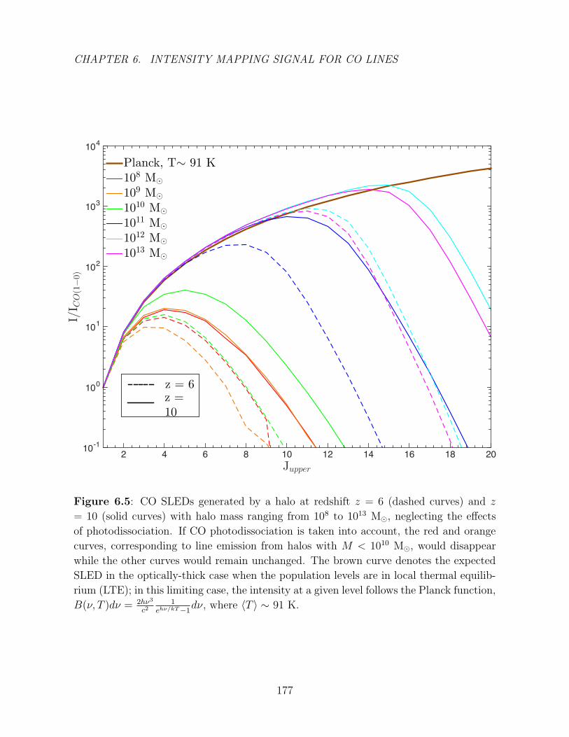
CHAPTER 6. INTENSITY MAPPING SIGNAL FOR CO LINES
Jupper2 4 6 8 10 12 14 16 18 20
I/I C
O(1−0)
10-1
100
101
102
103
104
Planck, T∼ 91 K108 M⊙
109 M⊙
1010 M⊙
1011 M⊙
1012 M⊙
1013 M⊙
z = 6z =10
Figure 6.5: CO SLEDs generated by a halo at redshift z = 6 (dashed curves) and z
= 10 (solid curves) with halo mass ranging from 108 to 1013 M, neglecting the effects
of photodissociation. If CO photodissociation is taken into account, the red and orange
curves, corresponding to line emission from halos with M < 1010 M, would disappear
while the other curves would remain unchanged. The brown curve denotes the expected
SLED in the optically-thick case when the population levels are in local thermal equilib-
rium (LTE); in this limiting case, the intensity at a given level follows the Planck function,
B(ν, T )dν = 2hν3
c21
ehν/kT−1dν, where 〈T 〉 ∼ 91 K.
177
CHAPTER 6. INTENSITY MAPPING SIGNAL FOR CO LINES
dissociation of CO in these molecular clouds where dust-shielding has grown inefficient.
However, the other curves, corresponding to line emission from higher mass halos that
have been normalized to the ground state, remain unchanged. This is due to the fact
that “turning on” photodissociation merely reduces the beam-averaged CO column
density according to eq. (6.32); since NCO controls the overall amplitude of the SLED
(and not the shape), adjusting this quantity simply amplifies or reduces the intensity of
all the CO lines by the same amount, leaving the ratio between lines unchanged.
As expected, we find that as the physical conditions in the emitting molecular clouds
grow more extreme, the CO rotational levels become increasingly populated and the
SLED rises accordingly. Consequently, the line intensities not only grow in magnitude,
but the peak of the CO SLED also shifts to higher J values, reflecting the excitation of
the more energetic states of the molecule.
The curves plotted in Figure 6.5 demonstrate this trend in the case where a UV duty
cycle of unity is assumed. In this scenario, the SFR and SFR surface density range from
10−4-1000 M yr−1 and 10−2-20 M yr−1 kpc−2 respectively, when the halo mass varies
from 108 to 1013 M (see figure 1). While the corresponding kinetic temperature remains
relatively constant for this ΣSFR range (Tkin ∼ 90 K), the H2 number density varies
significantly, 102 cm−3 . nH2 . 3× 105 cm−3. The variance in the shape of the CO SED
computed for fUV = 1 reflects this range of physical conditions parameterized by the
halo mass at z = 10; the SEDs produced by low-mass halos, M < 1010 M, peak at J '
4 before turning over and plummeting (neglecting CO photodissociation). In these low
density clouds, with correspondingly small velocity gradients (dv/dr ∼ 0.5 km s−1 pc−1)
and CO abundances (χCO ∼ 5×10⁻⁶), only the low-lying transitions such as CO J =
1→ 0 are optically thick. In contrast, in more extreme star-forming galaxies, i.e. M >
178
CHAPTER 6. INTENSITY MAPPING SIGNAL FOR CO LINES
1010 M, the H2 number densities reach ∼ 105 cm−3, the typical critical density value
for high-J CO emission. Consequently, the high-J lines grow optically thick and the line
ratios approach thermalization for transitions as high as J ∼ 13 in these high-mass halos.
6.4 Results
6.4.1 Predicted CO Fluxes and Spatially Averaged CO
Brightness Temperature
Given our LVG model of the full CO SLED, we can now predict the CO line fluxes
generated by a set of molecular clouds residing in a host halo of mass M at redshift z,
as well as compute the spatially averaged brightness temperature of any CO rotational
transition. The former is obtained by converting LVG-derived CO luminosities (eq.
(6.8)) into observed, velocity-integrated fluxes, FCO, using typical observer units,
LCOL
= 1.040× 10⁻³
(DL
Mpc
)2νobsGHz
FCOJy km s−1 (6.33)
where DL is the luminosity distance. The results are shown in Figure 6.6 for a range of
CO rotational lines emitted as a function of host halo mass at z = 6 (left panel) and z
= 10 (right panel). The dashed curves represent the fluxes obtained by including the
effects of CO photodissociation in our computations; as expected, the change in flux
when accounting for this phenomenon is most pronounced at the low-mass end where
FCO drops to zero once the CO is fully photodissociated. At the higher-mass end, we
predict that a ∼1011 M halo at redshift z = 6 will emit strongest in the J = 7 → 6
transition with a flux of ∼ 25 mJy while a halo with the same mass at z = 10 will emit
179

CHAPTER 6. INTENSITY MAPPING SIGNAL FOR CO LINES
FCO[Jykm/s]
10
-7
10
-6
10
-5
10
-4
10
-3
10
-2
10
-1
10
0
CO(1-0)
CO(3-2)
CO(5-4)
CO(7-6)
M[M
⊙]
10
81
09
10
10
10
11
10
12
10
13
10
-7
10
-6
10
-5
10
-4
10
-3
10
-2
10
-1
CO(2-1)
CO(4-3)
CO(6-5)
CO(8-7)
z =
6
PhotodissociationOFF
PhotodissociationON
FCO[Jykm/s]
10
-7
10
-6
10
-5
10
-4
10
-3
10
-2
10
-1
10
0
M[M
⊙]
10
81
09
10
10
10
11
10
12
10
13
10
-7
10
-6
10
-5
10
-4
10
-3
10
-2
10
-1
z =
10
Figure
6.6
:T
he
CO
rota
tion
alline
flux
asa
funct
ion
ofhal
om
ass
atz
=6
(lef
tpan
el)
andz
=10
(rig
ht
pan
el)
forJupper
=1-
8.Sol
idan
ddas
hed
curv
esden
ote
resu
lts
obta
ined
by
neg
lect
ing
(eq.
(6.3
1))
and
incl
udin
g(e
q.
(6.3
2))
the
effec
tsof
CO
phot
odis
soci
atio
n.
180
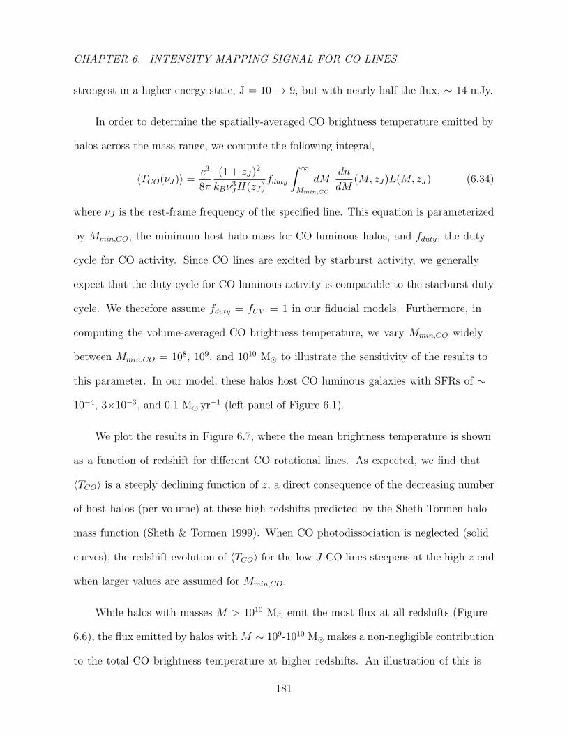
CHAPTER 6. INTENSITY MAPPING SIGNAL FOR CO LINES
strongest in a higher energy state, J = 10 → 9, but with nearly half the flux, ∼ 14 mJy.
In order to determine the spatially-averaged CO brightness temperature emitted by
halos across the mass range, we compute the following integral,
〈TCO(νJ)〉 =c3
8π
(1 + zJ)2
kBν3JH(zJ)
fduty
∫ ∞Mmin,CO
dMdn
dM(M, zJ)L(M, zJ) (6.34)
where νJ is the rest-frame frequency of the specified line. This equation is parameterized
by Mmin,CO, the minimum host halo mass for CO luminous halos, and fduty, the duty
cycle for CO activity. Since CO lines are excited by starburst activity, we generally
expect that the duty cycle for CO luminous activity is comparable to the starburst duty
cycle. We therefore assume fduty = fUV = 1 in our fiducial models. Furthermore, in
computing the volume-averaged CO brightness temperature, we vary Mmin,CO widely
between Mmin,CO = 108, 109, and 1010 M to illustrate the sensitivity of the results to
this parameter. In our model, these halos host CO luminous galaxies with SFRs of ∼
10−4, 3×10⁻³, and 0.1 M yr−1 (left panel of Figure 6.1).
We plot the results in Figure 6.7, where the mean brightness temperature is shown
as a function of redshift for different CO rotational lines. As expected, we find that
〈TCO〉 is a steeply declining function of z, a direct consequence of the decreasing number
of host halos (per volume) at these high redshifts predicted by the Sheth-Tormen halo
mass function (Sheth & Tormen 1999). When CO photodissociation is neglected (solid
curves), the redshift evolution of 〈TCO〉 for the low-J CO lines steepens at the high-z end
when larger values are assumed for Mmin,CO.
While halos with masses M > 1010 M emit the most flux at all redshifts (Figure
6.6), the flux emitted by halos with M ∼ 109-1010 M makes a non-negligible contribution
to the total CO brightness temperature at higher redshifts. An illustration of this is
181
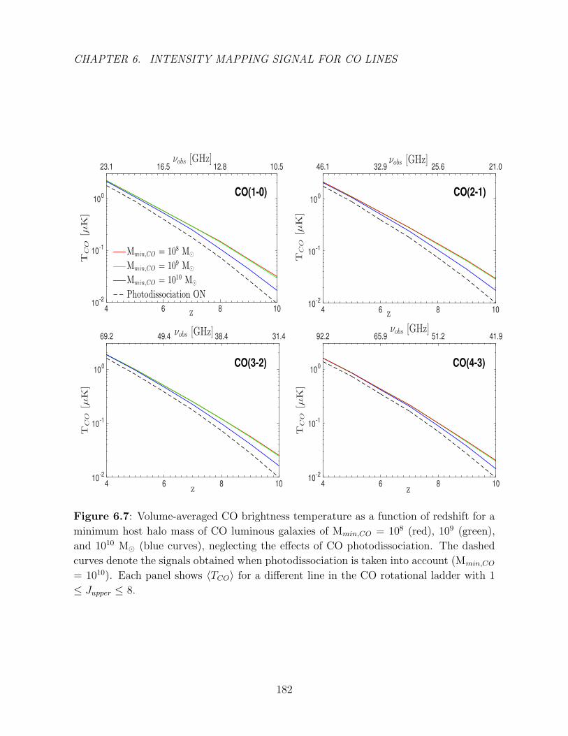
CHAPTER 6. INTENSITY MAPPING SIGNAL FOR CO LINES
νobs [GHz]23.1 16.5 12.8 10.5
z4 6 8 10
TCO[µK]
10-2
10-1
100
Mmin,CO = 108 M⊙
Mmin,CO = 109 M⊙
Mmin,CO = 1010 M⊙
Photodissociation ON
νobs [GHz]46.1 32.9 25.6 21.0
z4 6 8 10
TCO[µK]
10-2
10-1
100
νobs [GHz]69.2 49.4 38.4 31.4
z4 6 8 10
TCO[µK]
10-2
10-1
100
νobs [GHz]92.2 65.9 51.2 41.9
z4 6 8 10
TCO[µK]
10-2
10-1
100CO(3-2)
CO(1-0) CO(2-1)
CO(4-3)
Figure 6.7: Volume-averaged CO brightness temperature as a function of redshift for a
minimum host halo mass of CO luminous galaxies of Mmin,CO = 108 (red), 109 (green),
and 1010 M (blue curves), neglecting the effects of CO photodissociation. The dashed
curves denote the signals obtained when photodissociation is taken into account (Mmin,CO
= 1010). Each panel shows 〈TCO〉 for a different line in the CO rotational ladder with 1
≤ Jupper ≤ 8.
182

CHAPTER 6. INTENSITY MAPPING SIGNAL FOR CO LINES
νobs [GHz]115.3 82.3 64.0 52.4
z4 6 8 10
TCO[µK]
10-2
10-1
100
νobs [GHz]138.3 98.8 76.8 62.9
z4 6 8 10
TCO[µK]
10-2
10-1
100
νobs [GHz]161.4 115.3 89.7 73.4
z4 6 8 10
TCO[µK]
10-2
10-1
100
νobs [GHz]184.4 131.7 102.5 83.8
z4 6 8 10
TCO[µK]
10-2
10-1
100
CO(5-4)
CO(7-6)
CO(6-5)
CO(8-7)
Figure 6.7 (Continued)
183

CHAPTER 6. INTENSITY MAPPING SIGNAL FOR CO LINES
presented in Figure 6.8 which plots dT/d lnM , the contribution to the mean brightness
temperature per logarithmic halo mass for different CO lines as a function of halo mass
at z = 6 (dashed curves) and z = 10 (solid curves). It is clear that at z = 10, although
the primary component of the CO signal originates from halos with masses in the range
M ∼ 1010-1011 M, the CO emission from ∼ 109 M halos makes up nearly 15% of
the total signal for the low-J lines. Thus, raising the minimum host halo mass for CO
luminous halos from 108 M to 1010 M excludes a population of CO-emitting sources
and reduces the amplitude of 〈TCO〉 for the low-J lines by a factor of ∼ 2. The effects of
raising Mmin,CO vanish in the higher energy states since these low-mass halos emit less
than 1% of the total signal in these high-J lines; hence, the red, green, and blue solid
curves, denoting the mean brightness temperature for models where Mmin,CO = 108, 109,
and 1010 M, respectively, are barely distinguishable from one another for the higher
energy rotational transitions.
In the case where CO photodissociation is taken into account, we found that the
CO becomes fully photodissociated in halos with M < 1010 M (Figure 6.4); since these
low-mass halos do not emit CO flux in this model, the minimum host halo mass of a CO
luminous galaxy is effectively set to Mmin,CO = 1010 M. Accounting for CO destruction
in molecular clouds results in an overall reduction in the amplitude of 〈TCO〉, with the
low- and high-J lines weakening by ∼ 2-20% and 10-45%, respectively, over the range of
redshifts shown in Figure 6.7 (dashed curves).
The spatially averaged brightness temperature of the CO J = 1→ 0 line predicted
by our model assuming Mmin,CO = 108 M ranges from ∼ 0.6 µK at z = 6 to ∼ 0.03
µK at z = 10 when CO photodissociation is neglected. The strength of the CO signal
dwindles for higher-J lines, with 〈TCO(z = 6)〉 ∼ 0.3 µK and TCO(z = 10)〉 ∼ 0.1 µK for
184
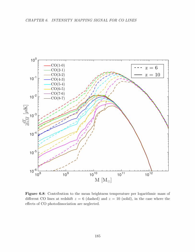
CHAPTER 6. INTENSITY MAPPING SIGNAL FOR CO LINES
M [M⊙]10
810
910
1010
1110
12
dT
dlnM
[µK]
10-6
10-5
10-4
10-3
10-2
10-1
100
CO(1-0)CO(2-1)CO(3-2)CO(4-3)CO(5-4)CO(6-5)CO(7-6)CO(8-7)
z = 6
z = 10
Figure 6.8: Contribution to the mean brightness temperature per logarithmic mass of
different CO lines at redshift z = 6 (dashed) and z = 10 (solid), in the case where the
effects of CO photodissociation are neglected.
185

CHAPTER 6. INTENSITY MAPPING SIGNAL FOR CO LINES
the CO J = 6→ 5 transition. “Turning on” photodissociation does not significantly effect
the mean brightness temperature of the high-J lines, but it does reduce the CO(1-0)
signal to 〈TCO〉 ∼ 0.4 and ∼ 0.01 µK at z = 6 and 10, respectively .
Without delving into any particular instrumental design, we briefly consider
the plausibility of detecting such signals. We use the radiometer equation for the
signal-to-noise ratio, S/N = (TCO/Tsys)√
∆ν tint where Tsys ∼ 20 K is the system
temperature of the detector, ∆ν is the observed bandwidth, and tint is the integration
time, which we take to be 1000 hours. We find that at z = 6, the predicted brightness
temperatures of the 4 lowest-lying CO transitions (neglecting CO photodissociation) can
be detected at 5σ confidence with a bandwidth of ∆ν ∼ 10 GHz, while a bandwidth of
∆ν ∼ 100 GHz is required for detection with 1σ confidence at z = 10. Higher J lines in
this model will require even longer integration times to achieve the desired brightness
sensitivity.
6.4.2 CO Power Spectrum
Given the existence of brighter foreground sources of emission at the relevant frequencies,
the mean redshifted CO signal will be difficult, if not impossible, to directly observe.
We therefore consider spatial fluctuations in the surface brightness and compute the
CO power spectrum predicted by different variations of our model. In contrast to the
spectrally smooth foreground sources, the CO signal is expected to have structure
in frequency space which can be used to isolate spatial fluctuations in its brightness
temperature. Since the power spectrum captures the underlying matter distribution and
structure, a map of the CO brightness temperature fluctuations at z ≥ 6 can be used to
186
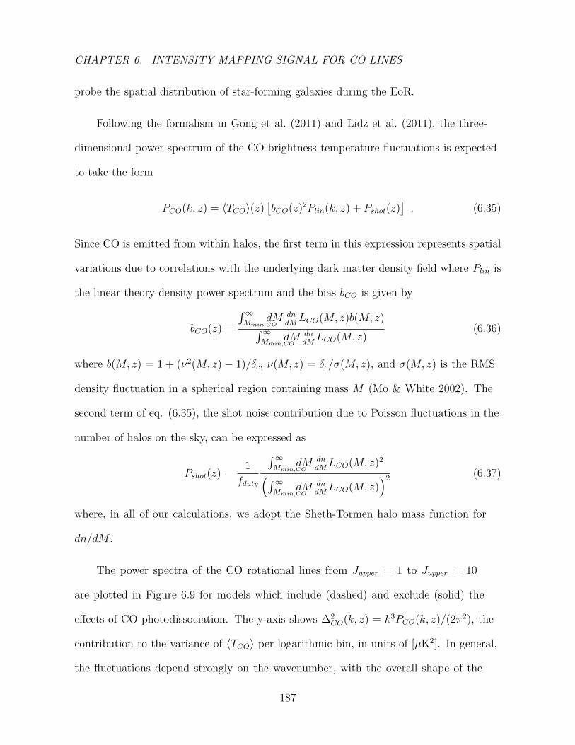
CHAPTER 6. INTENSITY MAPPING SIGNAL FOR CO LINES
probe the spatial distribution of star-forming galaxies during the EoR.
Following the formalism in Gong et al. (2011) and Lidz et al. (2011), the three-
dimensional power spectrum of the CO brightness temperature fluctuations is expected
to take the form
PCO(k, z) = 〈TCO〉(z)[bCO(z)2Plin(k, z) + Pshot(z)
]. (6.35)
Since CO is emitted from within halos, the first term in this expression represents spatial
variations due to correlations with the underlying dark matter density field where Plin is
the linear theory density power spectrum and the bias bCO is given by
bCO(z) =
∫∞Mmin,CO
dM dndMLCO(M, z)b(M, z)∫∞
Mmin,COdM dn
dMLCO(M, z)
(6.36)
where b(M, z) = 1 + (ν2(M, z) − 1)/δc, ν(M, z) = δc/σ(M, z), and σ(M, z) is the RMS
density fluctuation in a spherical region containing mass M (Mo & White 2002). The
second term of eq. (6.35), the shot noise contribution due to Poisson fluctuations in the
number of halos on the sky, can be expressed as
Pshot(z) =1
fduty
∫∞Mmin,CO
dM dndMLCO(M, z)2(∫∞
Mmin,COdM dn
dMLCO(M, z)
)2 (6.37)
where, in all of our calculations, we adopt the Sheth-Tormen halo mass function for
dn/dM .
The power spectra of the CO rotational lines from Jupper = 1 to Jupper = 10
are plotted in Figure 6.9 for models which include (dashed) and exclude (solid) the
effects of CO photodissociation. The y-axis shows ∆2CO(k, z) = k3PCO(k, z)/(2π2), the
contribution to the variance of 〈TCO〉 per logarithmic bin, in units of [µK2]. In general,
the fluctuations depend strongly on the wavenumber, with the overall shape of the
187

CHAPTER 6. INTENSITY MAPPING SIGNAL FOR CO LINES
k [Mpc−1]10
-210
-110
010
1
∆2 CO(k)[µK]2
10-4
10-3
10-2
10-1
100
101
102
z = 6
z = 10
Photodissociation OFFPhotodissociation ON
CO(1-0)
10-4
10-2
100
102
10-4
10-2
100
102
k [Mpc−1]10
-210
-110
010
1
∆2 CO(k)[µK]2
10-4
10-2
100
102
k [Mpc−1]10
-210
-110
010
1
∆2 CO(k)[µK]2
10-4
10-2
100
102
10-4
10-2
100
102
10-4
10-2
100
102
10-4
10-2
100
102
10-4
10-2
100
102
k [Mpc−1]10
-210
-110
010
1
∆2 CO(k)[µK]2
10-4
10-2
100
102
CO(4-3)
CO(3-2)
CO(5-4) CO(8-7)
CO(9-8)
CO(10-9)
CO(2-1)
CO(7-6)
CO(6-5)
Figure 6.9: Auto power spectrum of CO brightness temperature fluctuations for lines
all the way up to Jupper = 10, at z = 6 (red) and z = 10 (blue). In each panel, the solid
curves represent results for the models in which CO photodissociation was neglected and
a minimum host halo mass of MCO,min = 108 M was assumed; dashed curves denote
results for the case where the effects of CO photodissociation were included, effectively
setting the minimum host halo for CO luminous galaxies to MCO,min = 1010 M.
188
CHAPTER 6. INTENSITY MAPPING SIGNAL FOR CO LINES
predicted power spectra reflecting the form of eq. (6.35). On large scales, small k, the
clustering term dominates and the fluctuations in CO brightness temperature mirror the
underlying dark matter density field. Conversly, on small scales (large k), the shot noise
takes over and the fluctuations reach ∆2CO ∼ 300 - 1300 µK2 on scales of k = 10 Mpc−1
at z = 6, and ∆2CO ∼ 4 - 14 µK2 at z = 10 (when photodissociation is neglected). The J
= 1→ 0 transition is predicted to produce the strongest signal, with an amplitude that
drops by a factor of ∼5-50 across the wavenumber range k ∼ 10−2-10 Mpc−1 when the
higher energy state, J = 10→ 9, is considered instead.
The redshift evolution of ∆2CO is ultimately dictated by the behavior of 〈TCO〉(z);
although b2CO increases as the host halos become more clustered at higher redshifts, this
effect is not enough to compensate the declining brightness temperature with z. The
auto-correlation signal of all the CO lines therefore weakens as the redshift varies from z
= 6 to 10, dropping by ∼ 2 orders of magnitude over this redshift range. On the other
hand, our results for ∆2CO depend very weakly on our choice of the minimum host halo
mass for CO luminous galaxies; therefore, in the fiducial models where photodissociation
is neglected, we only plot results for the case where Mmin,CO = 108 M, thereby including
the contribution of the low-mass halos to the overall emission signal.
The effects of including CO photodissociation are most prominent for the low-J
lines, weakening the signal by, at most, a factor of ∼ 6 at z = 10 on large scales. At k =
0.1 Mpc−1, we find CO(1-0) brightness temperature fluctuations of amplitude ∆2CO ∼ 0.1
µK2 at z = 6, whether or not CO photodissociation is taken into account. At z = 10,
∆2CO(k = 0.1 Mpc−1) ∼ 5×10⁻⁴ and 8×10⁻⁵ µK2 for the J = 1→ 0 line in the models
where photodissociation is turned “off” (assuming fixed Mmin,CO = 108 M) and “on”,
respectively.
189
CHAPTER 6. INTENSITY MAPPING SIGNAL FOR CO LINES
6.5 Discussion
We have presented a new approach to estimating the mean CO emission signal from the
epoch of reionization (EoR) that links the atomic physics of molecular emission lines
to high-redshift observations of star-forming galaxies. This method is based on LVG
modeling, a radiative transfer modeling technique that generates the full CO SLED for
a specified set of characterizing parameters, namely, the kinetic temperature, number
density, velocity gradient, CO abundance, and column density of the emitting source.
We showed that these LVG parameters, which dictate both the shape and amplitude of
the CO SLED, can be expressed in terms of the emitting galaxy’s global star formation
rate, SFR, and the star formation rate surface density, ΣSFR. Employing the SFR-M
relation empirically derived for high-redshift galaxies, i.e. z ≥ 4, we can then ultimately
express the LVG parameters, and thus, the specific intensity of any CO rotational line,
as functions of the host halo mass M and redshift z.
Adopting a starburst duty cycle of fUV = 1, the average SFR−M relation derived
via abundance-matching for 4 < z < 8 is characterized by a steeply declining slope at
the low-mass end, where the star formation rate goes as SFR ∝ M1.6. With the SFR
dropping to values below 0.1 M yr−1 for M < 1010 M, the physical conditions in
these low-mass halos are not “extreme” enough to substantially excite the high-J CO
rotational states. The resulting CO SLEDs correspondingly peak around J ' 4 before
turning over, and the overall contribution of CO emission from this halo population
grows negligible at lower redshifts. On the other hand, the H2 number density and
CO-to-H2 abundance in halos with masses M ≥ 1010 M are large enough to keep the
high-J population levels thermalized; the CO SLEDs generated by these massive halos
190
CHAPTER 6. INTENSITY MAPPING SIGNAL FOR CO LINES
therefore have peaks shifited to J ≥ 10 and overall higher amplitudes, reflecting the
excitation of the more energetic states of the molecule.
We also consider the effects of CO photodissociation on the CO line intensities
generated by our fiducial models. Assuming that the threshold for CO survival is set by
a universal dust opacity, we adopt a first-order approximation of NCO which effectively
reduces the CO column density with decreasing metallicity. In the limiting case where
the metallicity drops so low that there is not enough dust to shield CO, the CO is
considered fully dissociated and NCO is set to zero. We find that such conditions occur
in halos with M . 1010 M, causing the line intensities emitted by these low-mass halos
to entirely disappear in models where CO photodissociation is accounted for.
Given our LVG model of the full CO SLEDs, we can predict both FCO, the CO line
flux generated by a set of molecular clouds in a host halo of mass M at redshift z, as well
as 〈TCO〉, the spatially averaged brightness temperature of any CO rotational transition.
We find that the flux emitted in the J = 1 → 0 transition by a halo at redshift z = 6
with mass M ∼ 1011 M is FCO(1−0) ∼ 0.8 mJy km/s. The higher rotational lines are
expected to be even brighter, with a 1011 M halo at z = 6 emitting a CO(6-5) flux of ∼
23 mJy km/s. These fluxes drop by 25-30% when considering a 1011 M halo emitting
at z = 10, with FCO(1−0) ∼ 0.2 mJy km/s and FCO(6−5) ∼ 7 mJy km/s.
The CO line fluxes emitted by individual host halos of mass M at redshift z
as estimated in this paper, are found to be generally higher than previous estimates
obtained in the literature (Obreschkow et al. 2009; Munoz & Furlanetto 2013). Building
an analytic formalism within a paradigm where star formation is a function of gas supply
and stellar feedback, the model presented in Munoz & Furlanetto (2013) provides radial
191
CHAPTER 6. INTENSITY MAPPING SIGNAL FOR CO LINES
distributions of SFR, Σgas, and T which are then used to calculate the masses, sizes,
and number of GMCs, and the corresponding total CO line luminosities emitted by
these clouds. Consequently, the CO(1-0) flux emitted by a 1011 M halo at z = 6 as
predicted by this model is ∼ 0.01-0.03 mJy km/s, an order of magnitude smaller than
the flux estimates derived with our methodology. The flux in the J = 6 → 5 transition
is found to be highly sensitive to the inclusion of turbulent clumps within the GMCs,
given that the high densities in such inhomogeneities can effect the thermalization of the
higher-J rotational lines; the resulting CO(6-5) flux in the models presented in Munoz
& Furlanetto (2013) thus varies from 10 mJy km/s to 10−3 mJy km/s when turbulent
clumps are included and excluded, respectively.
While these results are comparable to those derived using the semi-analytic methods
of Obreschkow et al. (2009), they are consistently smaller than the values presented in
this paper. The prolific number of parameters used to characterize the GMC properties
in Munoz & Furlanetto (2013) make it difficult to ascertain the source of divergence
between our results, which both use radiative transfer techniques. However, we suspect
these differences can be traced back to the different prescriptions used to set the star
formation rate surface density, ΣSFR, and gas surface density, Σgas, the two ingredients
which, once related to one another via the Kennicutt-Schmidt relation in our model,
determine the shape and amplitude of the resulting CO SLED. Furthermore, Munoz &
Furlanetto (2013) parameterizes the properties of MCs as a function of their position
relative to the disk center, and after considering the level populations and optical depth
of CO in each cloud directly, computes the resulting flux from the entire galaxy by
counting up the number of clouds at each galactic radius. The molecular clouds in our
model, on the other hand, are characterized by disk-averaged properties of the host
192

CHAPTER 6. INTENSITY MAPPING SIGNAL FOR CO LINES
halo disk; to derive the signal from a CO-emitting galaxy, we assume a large number
of these identical homogeneous collapsing clouds and scale the line intensities with the
disk-averaged CO column density. Based on the sensitivity limits quoted in Munoz &
Furlanetto (2013), our approach predicts that the Jupper = 1 line in z = 6 halos with
mass M ≥ 1012 M will be observable by JVLA2(Jansky Very Large Array) after ten
hours of observation; at this redshift, the CO(2-1) and CO(3-2) lines fluxes emitted by
halos with M > 1011 M are also expected to be observed by JVLA. Similarly, we expect
ALMA to detect the CO(6-5) flux emitted by z = 6 halos with mass M ≥ 5×10¹⁰ M
after ten hours of observation, and higher rotational lines Jupper ≥ 7 emitted by halos
with M & 1011 M.
To obtain an estimate of the spatially averaged brightness temperature of a given
line at a particular redshift, we simply integrate LCO(M, z) over the range of halo masses
that are expected to host CO-luminous galaxies. In the case where CO photodissociation
is included, the minimum host halo mass of CO-emitting galaxies is set to MCO,min ∼
1010 M by the model itself, since the CO is found to be fully dissociated in halos with
M < 1010 M. When CO photodissociation is ignored, varying MCO,min from 108 to 1010
M reduces the low-J line signals at high redshifts, where the CO emission from ∼ 109
M halos make up a non-negligible percentage of the total emission.
In our fiducial model where CO photodissociation is neglected and Mmin,CO = 108
M, we predict a spatially averaged brightness temperature of 〈TCO〉 ∼ 0.5 µK at z = 6
and 0.03 µK at z = 10 for the low-J CO rotational lines, with brightness temperature
fluctuations of amplitude ∆2CO ∼ 0.1 and 0.005 µK2 respectively, at k = 0.1 Mpc−1.
2http://www.vla.nrao.edu/
193

CHAPTER 6. INTENSITY MAPPING SIGNAL FOR CO LINES
These CO emission signals are further reduced to 〈TCO〉 ∼ 0.4 and 0.01 µK at z = 6 and
10, respectively, for the low-lying states when the effects of CO photodissociation are
included in the calculations. (Note that, since CO lines are typically excited by starburst
activity, the choice of Mmin,CO = 108 M is favored by theoretical and numerical
investigations which indicate that 108 M is the minimum mass required for a halo to
cool and form stars at these high redshifts (Haiman et al. 1996; Tegmark et al. 1997;
Trenti et al. 2010; Loeb & Furlanetto 2013)). Our estimates of 〈TCO〉 for the low-J CO
transitions are comparable to the values obtained in previous work by Carilli (2011),
Gong et al. (2011), Lidz et al. (2011), and Pullen et al. (2013). Constructing a model
based on the required cosmic star formation rate density to reionize the universe, Carilli
(2011) obtains an order-of-magnitude estimate of 〈TCO〉(z = 8) ∼ 1 µK for the J =
1→ 0 and J = 2→ 1 transitions. Gong et al. (2011) arrives at a slightly smaller estimate
of the CO(1-0) brightness temperature, 〈TCO〉 ∼ 0.5 µK for z = 6 and 0.1 µK for z =
10, by using the Millennium numerical simulation results of Obreschkow et al. (2009) to
model the CO emission from high-redshift galaxies. Lidz et al. (2011) assumes a linear
SFR−M relation and a set of low-z empirical scaling relations between a galaxy’s SFR,
LFIR, and LCO(1−0) to estimate 〈TCO〉 for these low-J lines; they find a mean brightness
temperature of ∼ 2 µK at z ∼ 6 and 0.5 µK at z ∼ 10 with fluctuations ∆2CO ∼ 0.2 and
0.02 µK2, respectively, on scales of k ∼ 0.1 Mpc−1. In a more recent paper, Pullen et al.
(2013) follows the approach taken in Lidz et al. (2011) with a few adjustments to the
SFR −M prescription to arrive at brightness temperatures of 〈TCO〉 ∼ 0.7 and 0.2 µK
at redshifts z = 6 and 10 respectively, assuming Mmin,CO = 109 M for the CO(1-0) and
CO(2-1) lines.
While these previous works are limited almost exclusively to predicting the signals
194

CHAPTER 6. INTENSITY MAPPING SIGNAL FOR CO LINES
of the 12CO J=1→0 and 2→1 transition lines, our LVG-based approach generates the
full CO SLED and thus allows us to compute the signal strength of the higher-J energy
states as well. For example, we predict a CO(10-9) brightness temperature of 〈TCO〉 ∼
0.05 µK at z = 6 and 0.003 µK at z = 10 with ∆2CO(k = 0.1) ∼ 0.003 and 10−5µK2
respectively. We look forward to future experiments, such as the Carbon MonOxide
Mapping Array (COMA)3 currently under development, which promise to provide
spectral-spatial intensity mapping of CO at the high redshifts characterizing the epoch
of reionization.
6.6 Acknowledgements
We thank Reinhard Genzel for helpful discussions and suggestions.This work was
supported by the Raymond and Beverly Sackler Tel Aviv University-Harvard/ITC
Astronomy Program. A.L. acknowledges support from the Sackler Professorship by
Special Appointment at Tel Aviv University. This work was also supported in part by
a PBC Israel Science Foundation I-CORE Program grant 1829/12, and in part by NSF
grant AST-1312034. This material is based upon work supported by the National Science
Foundation Graduate Research Fellowship under Grant No. DGE1144152. Any opinion,
findings, and conclusions or recommendations expressed in this material are those of the
authors and do not necessarily reflect the views of the National Science Foundation.
3http://www.stanford.edu/group/church_group/cgi-bin/wordpress/?page_id=515
195
Chapter 7
Spectral Distortion of the CMB by
the Cumulative CO Emission from
Galaxies throughout Cosmic History
This thesis chapter originally appeared in the literature as
N. Mashian, A. Loeb, and A. Sternberg, Spectral distortion
of the CMB by the cumulative CO emission from galaxies
throughout cosmic history, Monthly Notices of the Royal
Astronomical Society, 458, L99, 2016
7.1 Abstract
We show that the cumulative CO emission from galaxies throughout cosmic history
distorts the spectrum of the cosmic microwave background (CMB) at a level that is
196
CHAPTER 7. SPECTRAL DISTORTION BY CUMULATIVE CO EMISSION
well above the detection limit of future instruments, such as the Primordial Inflation
Explorer (PIXIE). The modeled CO signal has a prominent bump in the frequency
interval 100-200 GHz, with a characteristic peak intensity of ∼ 2×10⁻²³ W m−2 Hz−1 sr−1.
Most of the CO foreground originates from modest redshifts, z ∼ 2-5, and needs to be
efficiently removed for more subtle distortions from the earlier universe to be detected.
7.2 Introduction
Since the measurements by COBE/Far Infrared Absolute Spectrophotometer (FIRAS),
the average cosmic microwave background spectrum (CMB) spectrum is known to be
extremely close to a perfect blackbody with a temperature T0 = 2.726±0.001 K and
no detected global spectral distortions to date (Mather et al. 1994; Fixsen et al. 1996;
Fixsen 2009). However, the standard model of cosmology predicts tiny deviations from
the Planckian spectrum due to cosmological processes which heat, cool, scatter, and
create CMB photons throughout the history of the Universe (Sunyaev & Zeldovich
1969; Zeldovich & Sunyaev 1969; Sunyaev & Zeldovich 1970; Illarionov & Siuniaev
1975a,b; Danese & de Zotti 1982; Burigana et al. 1991; Hu & Silk 1993; Burigana &
Salvaterra 2003; Chluba et al. 2012; Sunyaev & Khatri 2013). While at redshifts z &
2×10⁶, the thermalization process (mediated by the combined action of double Compton
emission, Bremsstrahlung and Compton scattering) is rapid enough to efficiently erase
any distortion to unobservable levels, at lower redshifts, the CMB spectrum becomes
vulnerable and spectral distortions that form are “locked in” and can thus be theoretically
observed today (Chluba & Sunyaev 2012; Chluba 2014; Chluba et al. 2015).
In connection with early energy release, two types of CMB distortions are
197
CHAPTER 7. SPECTRAL DISTORTION BY CUMULATIVE CO EMISSION
traditionally distinguished: chemical potential µ- and Compton y- distortions (Sunyaev
& Zeldovich 1969, 1970; Illarionov & Siuniaev 1975a,b). In the regime 2×10⁶ . z .
3×10⁵, the efficiency of double Compton and Bremsstrahlung processes in controlling the
number of CMB photons gradually reduces while photons are still efficiently redistributed
in energy by the Compton process. In this case, where thermalization stops being
complete, electrons and photons are in kinetic equilibrium with respect to Compton
scattering, and any energy injection produces a chemical potential characterized by
µ(ν). At lower redshifts, z . 104, up-scattering of photons by electrons also becomes
inefficient and photos diffuse only little in energy, creating a y-type distortion y(ν) which
is an early-universe analogue of the thermal Sunyaev-Zeldovich effect. Both types of
distortions are tightly constrained by COBE/FIRAS measurements, with upper limits of
|µ| < 9×10⁻⁵ and |y| < 1.5×10⁻⁵ at 95% confidence (Fixsen et al. 1996).
The amplitude of these signals, predicted within the standard cosmological
paradigm, is expected to fall below the bounds set by COBE-FIRAS measurements.
The average amplitude of the y-parameter, due to the large-scale structure and the
reionization epoch, is expected to be y ' 10−7-10−6, with the most recent computations
predicting y ' 2×10⁻⁶ (Hu et al. 1994b; Refregier et al. 2000; Oh et al. 2003; Hill et al.
2015). The µ-distortion signal is expected to be even weaker, with the damping of
small-scale acoustic modes giving rise to µ ' 2×10⁻⁸ in the standard slow-roll inflation
scenario (Daly 1991; Hu et al. 1994a; Chluba et al. 2012). Although these distortions
are small, significant progress in technology in the last two decades promises to detect
these spectral distortions. Experimental concepts, like the Primordial Inflation Explorer
(PIXIE; Kogut et al. 2011a) and Polarized Radiation Imaging and Spectroscopy Mission
(PRISM; Andre et al. 2014), could possibly improve the absolute spectral sensitivity
198
CHAPTER 7. SPECTRAL DISTORTION BY CUMULATIVE CO EMISSION
limits of COBE/FIRAS by 2-3 orders of magnitude and detect the aforementioned
signals at the 5σ level, providing measurements at sensitivities µ = 5×10⁻⁸ for a chemical
potential distortion and y = 10−8 for a Compton distortion (Fixsen & Mather 2002;
Kogut et al. 2011a; Chluba 2013; Chluba & Jeong 2014).
However, it is not yet clear what the foreground limitations to measuring these
primordial spectral distortions will be. When considering the large angular scales of
interest to PIXIE, focus has been geared towards the foreground subtraction of polarized
emission from the Milky Way’s interstellar medium (ISM) which is dominated by
synchrotron radiation from cosmic ray electrons accelerated in the Galactic magnetic
field, and thermal emission from dust grains. Kogut et al. (2011b) claim that the
CMB emission can be distinguished from Galactic foregrounds based on their different
frequency spectra, as long as the number of independent frequency channels equals or
exceeds the number of free parameters to be derived from a multi-frequency fit.
But in addition to these Galactic foregrounds, there is another contaminant which
has been primarily neglected in the literature, and that is the diffuse background of CO
emission lines from external galaxies. Until recently, Righi et al. (2008) provided the
only estimate of this redshift-integrated CO emission signal. Assuming star formation is
driven by major mergers, they calculated the resulting star-formation rate (SFR) and
then converted it to a CO luminosity, LCO, using the measured ratio of LCO to SFR in
M82, a low-redshift starburst galaxy. The CO background they found, integrated over all
redshifts, is expected to contribute ∼ 1 µK at ν & 100 GHz with an almost flat spectrum.
De Zotti et al. (2016) also include estimates of the background contributed by CO lines
from star-forming galaxies when they consider the Galactic and extragalactic foreground
intensity compared with the CMB spectra. Using the LIR-LCO relations presented in
199

CHAPTER 7. SPECTRAL DISTORTION BY CUMULATIVE CO EMISSION
Greve et al. (2014) for the CO rotational ladder from J = 1→ 0 to J = 5→ 4, they find
that the CO signal is substantially higher than the PIXIE sensitivity, with the CO(4-3)
line alone contributing ∼ 3×10⁻²⁴ erg s−1 cm−2 sr−1 at sub-mm wavelengths.
In this paper, we apply the formalism and machinery presented in Mashian et al.
(2015a) to predict the total CO emission signal generated by a population of star-forming
halos with masses M ≥ 1010 M from the present-day, to redshifts as early as z ∼
15. Our comprehensive approach is based on large-velocity gradient (LVG) modeling,
a radiative transfer modeling technique that produces the full CO spectral line energy
distribution (SLED) for a specified set of parameters characterizing the emitting source.
By linking these parameters to the global properties of the host halos, we calculate the
CO line intensities emitted by a halo of mass M at redshift z, and then further integrate
these CO luminosities over the range of halo masses hosting CO-luminous galaxies to
derive the average surface brightness of each rotational line. We find that over a range
of frequencies (30-300 GHz) spanned by a PIXIE-like mission, the signal strength of this
diffuse background is 1-3 orders of magnitude larger than the spectral distortion limits
PIXIE aims to provide. The CO foreground must be removed in order for the more
subtle distortion signals from the earlier universe to be detected.
This Letter is organized as follows. Section 7.3 provides a brief overview of the
formalism and key ingredients of our CO-signal modeling technique. Section 7.4 presents
the results and Section 7.5 summarizes the main conclusions. We adopt a flat, ΛCDM
cosmology with Ωm = 0.3, ΩΛ = 0.7, Ωb = 0.045, H0 = 70 km s−1Mpc−1 (i.e. h = 0.7),
σ8 = 0.82, and ns = 0.95, consistent with the most recent measurements from Planck
(Planck Collaboration et al. 2016b).
200
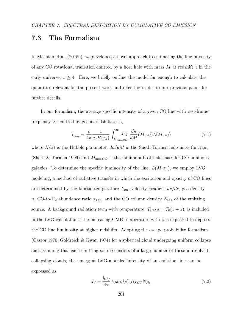
CHAPTER 7. SPECTRAL DISTORTION BY CUMULATIVE CO EMISSION
7.3 The Formalism
In Mashian et al. (2015a), we developed a novel approach to estimating the line intensity
of any CO rotational transition emitted by a host halo with mass M at redshift z in the
early universe, z ≥ 4. Here, we briefly outline the model far enough to calculate the
quantities relevant for the present work and refer the reader to our previous paper for
further details.
In our formalism, the average specific intensity of a given CO line with rest-frame
frequency νJ emitted by gas at redshift zJ is,
Iνobs =c
4π
1
νJH(zJ)
∫ ∞Mmin,CO
dMdn
dM(M, zJ)L(M, zJ) (7.1)
where H(z) is the Hubble parameter, dn/dM is the Sheth-Tormen halo mass function
(Sheth & Tormen 1999) and Mmin,CO is the minimum host halo mass for CO-luminous
galaxies. To determine the specific luminosity of the line, L(M, zJ), we employ LVG
modeling, a method of radiative transfer in which the excitation and opacity of CO lines
are determined by the kinetic temperature Tkin, velocity gradient dv/dr, gas density
n, CO-to-H2 abundance ratio χCO, and the CO column density NCO of the emitting
source. A background radiation term with temperature, TCMB = T0(1 + z), is included
in the LVG calculations; the increasing CMB temperature with z is expected to depress
the CO line luminosity at higher redshifts. Adopting the escape probability formalism
(Castor 1970; Goldreich & Kwan 1974) for a spherical cloud undergoing uniform collapse
and assuming that each emitting source consists of a large number of these unresolved
collapsing clouds, the emergent LVG-modeled intensity of an emission line can be
expressed as
IJ =hνJ4π
AJxJβJ(τJ)χCONH2 (7.2)
201

CHAPTER 7. SPECTRAL DISTORTION BY CUMULATIVE CO EMISSION
where xJ is the population fraction in the J th level, AJ is the Einstein radiative
coefficient, NH2 is the beam-averaged H2 column density, and βJ = (1 − eτJ )/τJ is
the photon-escape probability. To carry out these computations, we use the Mark &
Sternberg LVG radiative transfer code described in Davies et al. (2012).
We showed previously that the LVG parameters, Tkin, nH2 , dv/dr, χCO, and NH2
, which drive the physics of CO transitions and ultimately dictate both the shape and
amplitude of the resulting CO SLED, can be linked to the emitting galaxy’s global star
formation rate, SFR, and the star formation rate surface density, ΣSFR. The analytic
expressions for these quantities can be found in section 2.3 of Mashian et al. (2015a),
and will not be rederived here. The final ingredient in our model is thus a SFR −M
relation that allows us to express these LVG parameters solely as functions of the global
properties of the host halo, i.e. the halo mass M and redshift z.
For high redshifts, z ≥ 4, we adopt the average SFR −M relation derived in
Mashian et al. (2016) via abundance-matching. Assuming each dark-matter halo hosts
a single galaxy, they mapped the shape of the observed ultraviolet luminosity functions
(UV LFs) at z ∼ 4-8 to that of the halo mass function at the respective redshifts and
found that the SFR −M scaling law is roughly constant across this redshift range
(within 0.2 dex). This average relation, which faithfully reproduces the observed z ∼ 9
- 10 LFs, is therefore employed in our calculations for all redshifts greater than 4. For
z < 4, we rely on the results of Behroozi et al. (2013b,a) which empirically quantified
the stellar mass history of dark matter halos, using a comprehensive compilation of
observational data along with simulated halo merger trees to constrain a parameterized
stellar mass-halo mass relation.
202
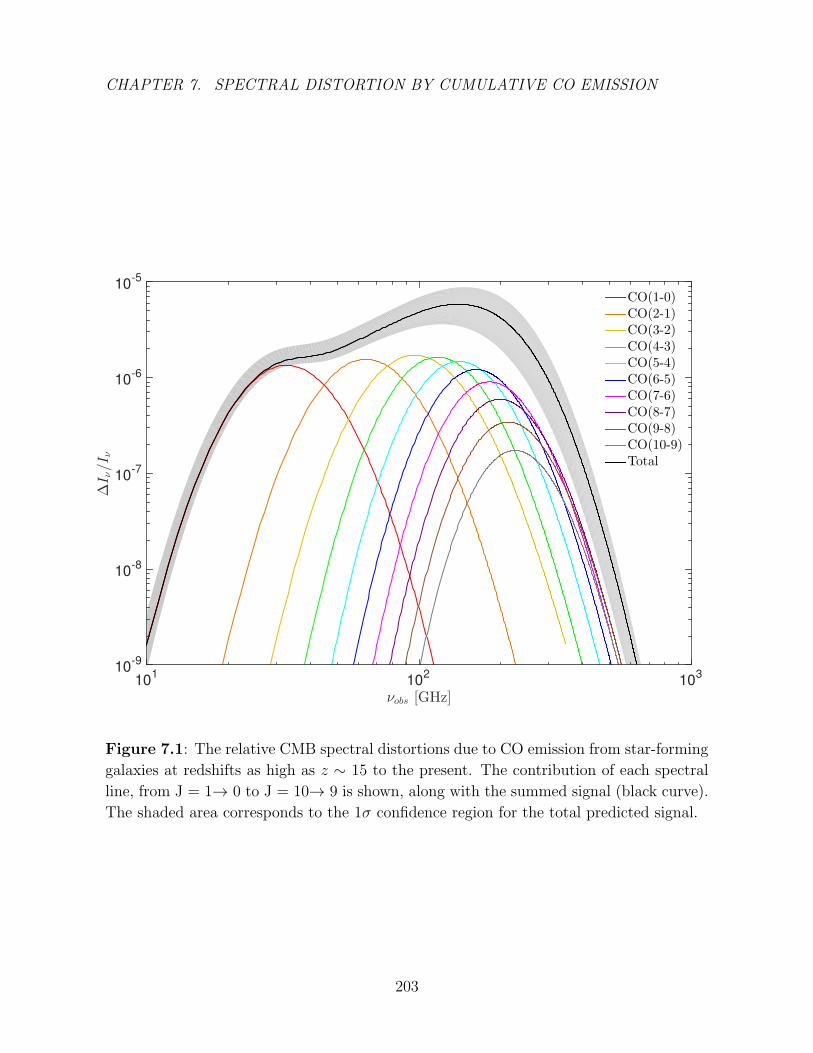
CHAPTER 7. SPECTRAL DISTORTION BY CUMULATIVE CO EMISSION
νobs [GHz]10
110
210
3
∆I ν/I ν
10-9
10-8
10-7
10-6
10-5
CO(1-0)CO(2-1)CO(3-2)CO(4-3)CO(5-4)CO(6-5)CO(7-6)CO(8-7)CO(9-8)CO(10-9)Total
Figure 7.1: The relative CMB spectral distortions due to CO emission from star-forming
galaxies at redshifts as high as z ∼ 15 to the present. The contribution of each spectral
line, from J = 1→ 0 to J = 10→ 9 is shown, along with the summed signal (black curve).
The shaded area corresponds to the 1σ confidence region for the total predicted signal.
203

CHAPTER 7. SPECTRAL DISTORTION BY CUMULATIVE CO EMISSION
7.4 Results
In Figure 7.1, we present our predictions of the contribution of each spectral line to the
cumulative CO background from star-forming galaxies at redshifts as high as z ∼ 15
to the present. The low-J CO lines peak at frequencies corresponding to an emission
redshift of z ∼ 2. This emission is dominated by star-forming halos with masses 1011-1012
M, hosting molecular clouds that are characterized by a gas kinetic temperature Tkin ∼
40 K and H2 number densities nH2 ∼ 100 - 1000 cm−3. The higher-J (J > 5) CO
signal is dominated by emission from 1011-1012 M host halos residing at z & 4; in the
star-forming galaxies at these high redshifts, the physical conditions in the emitting
molecular clouds are extreme enough to thermalize the higher-order CO transitions, with
gas kinetic temperatures of ∼ 60 K and number densities of order 104 cm−3. Integrating
over the population of CO luminous halos between redshifts 0 ≤ z ≤ 15, we find that
the total emission (black curve) predicted by our LVG-based model is not completely
spectrally smooth, but rather has a prominent bump in the frequency interval ∼ 100 - 200
GHz with a characteristic peak intensity of ∼ 2×10⁻²³ W m−2 Hz−1 sr−1, i.e. ∆Iν/Iν '
(5±2)×10−6. This is the frequency range within which the most prominent redshifted
CO line emissions, originating from sources at redshifts z ∼ 2 - 5, fall and accumulate to
form the peak in the cumulative signal depicted in Figure 7.1. The total CO intensity
is ∼ 0.01% of the far-infrared background intensity computed in Fixsen et al. (1998)
and Lutz (2014), where the former computes a total 125-2000 µm background of ∼ 14
nW m−2sr−1 and the latter computes a total 8-1000 µm background of ∼ 27 nW m−2sr−1.
The uncertainty in our estimates of the CO signal, represented by the shaded regions in
Figures 7.1-7.3, primarily stems from the uncertainty in the average SFR−M relations
204
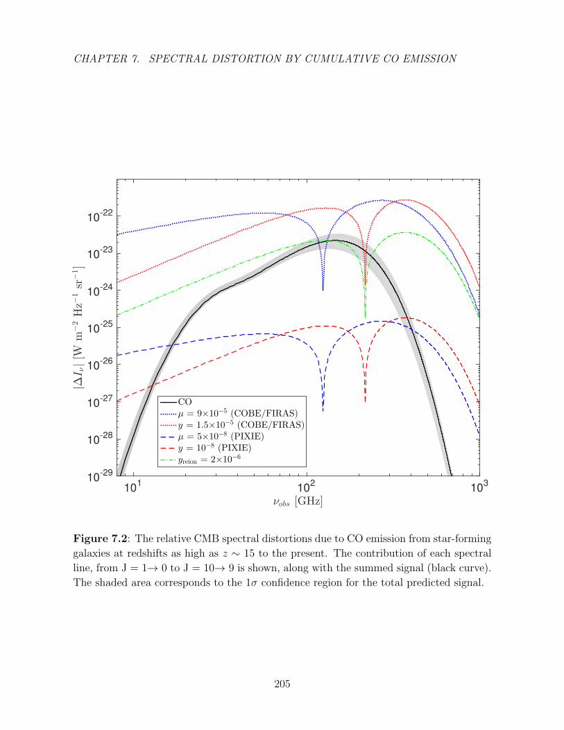
CHAPTER 7. SPECTRAL DISTORTION BY CUMULATIVE CO EMISSION
νobs [GHz]10
110
210
3
|∆I ν|[W
m−2Hz−
1sr
−1]
10-29
10-28
10-27
10-26
10-25
10-24
10-23
10-22
COµ = 9×10⁻⁵ (COBE/FIRAS)y = 1.5×10⁻⁵ (COBE/FIRAS)µ = 5×10⁻⁸ (PIXIE)y = 10−8 (PIXIE)yreion = 2×10⁻⁶
Figure 7.2: The relative CMB spectral distortions due to CO emission from star-forming
galaxies at redshifts as high as z ∼ 15 to the present. The contribution of each spectral
line, from J = 1→ 0 to J = 10→ 9 is shown, along with the summed signal (black curve).
The shaded area corresponds to the 1σ confidence region for the total predicted signal.
205
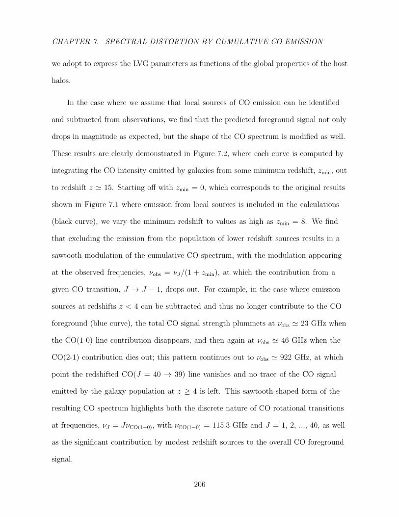
CHAPTER 7. SPECTRAL DISTORTION BY CUMULATIVE CO EMISSION
we adopt to express the LVG parameters as functions of the global properties of the host
halos.
In the case where we assume that local sources of CO emission can be identified
and subtracted from observations, we find that the predicted foreground signal not only
drops in magnitude as expected, but the shape of the CO spectrum is modified as well.
These results are clearly demonstrated in Figure 7.2, where each curve is computed by
integrating the CO intensity emitted by galaxies from some minimum redshift, zmin, out
to redshift z ' 15. Starting off with zmin = 0, which corresponds to the original results
shown in Figure 7.1 where emission from local sources is included in the calculations
(black curve), we vary the minimum redshift to values as high as zmin = 8. We find
that excluding the emission from the population of lower redshift sources results in a
sawtooth modulation of the cumulative CO spectrum, with the modulation appearing
at the observed frequencies, νobs = νJ/(1 + zmin), at which the contribution from a
given CO transition, J → J − 1, drops out. For example, in the case where emission
sources at redshifts z < 4 can be subtracted and thus no longer contribute to the CO
foreground (blue curve), the total CO signal strength plummets at νobs ' 23 GHz when
the CO(1-0) line contribution disappears, and then again at νobs ' 46 GHz when the
CO(2-1) contribution dies out; this pattern continues out to νobs ' 922 GHz, at which
point the redshifted CO(J = 40 → 39) line vanishes and no trace of the CO signal
emitted by the galaxy population at z ≥ 4 is left. This sawtooth-shaped form of the
resulting CO spectrum highlights both the discrete nature of CO rotational transitions
at frequencies, νJ = JνCO(1−0), with νCO(1−0) = 115.3 GHz and J = 1, 2, ..., 40, as well
as the significant contribution by modest redshift sources to the overall CO foreground
signal.
206
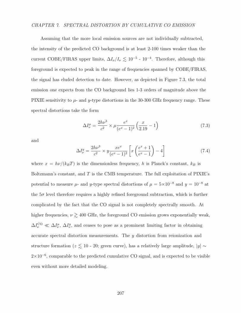
CHAPTER 7. SPECTRAL DISTORTION BY CUMULATIVE CO EMISSION
Assuming that the more local emission sources are not individually subtracted,
the intensity of the predicted CO background is at least 2-100 times weaker than the
current COBE/FIRAS upper limits, ∆Iν/Iν . 10−5 - 10−4. Therefore, although this
foreground is expected to peak in the range of frequencies spanned by COBE/FIRAS,
the signal has eluded detection to date. However, as depicted in Figure 7.3, the total
emission one expects from the CO background lies 1-3 orders of magnitude above the
PIXIE sensitivity to µ- and y-type distortions in the 30-300 GHz frequency range. These
spectral distortions take the form
∆Iµν =2hν3
c2× µ ex
(ex − 1)2
( x
2.19− 1)
(7.3)
and
∆Iyν =2hν3
c2× y xex
(ex − 1)2
[x
(ex + 1
ex − 1
)− 4
](7.4)
where x = hν/(kBT ) is the dimensionless frequency, h is Planck’s constant, kB is
Boltzmann’s constant, and T is the CMB temperature. The full exploitation of PIXIE’s
potential to measure µ- and y-type spectral distortions of µ = 5×10⁻⁸ and y = 10−8 at
the 5σ level therefore requires a highly refined foreground subtraction, which is further
complicated by the fact that the CO signal is not completely spectrally smooth. At
higher frequencies, ν & 400 GHz, the foreground CO emission grows exponentially weak,
∆ICOν ∆Iµν , ∆Iyν , and ceases to pose as a prominent limiting factor in obtaining
accurate spectral distortion measurements. The y distortion from reionization and
structure formation (z . 10 - 20; green curve), has a relatively large amplitude, |y| ∼
2×10⁻⁶, comparable to the predicted cumulative CO signal, and is expected to be visible
even without more detailed modeling.
207
CHAPTER 7. SPECTRAL DISTORTION BY CUMULATIVE CO EMISSION
νobs [GHz]10
110
210
3
∆I ν/I ν
10-11
10-10
10-9
10-8
10-7
10-6
10-5
zmin = 0zmin = 1zmin = 2zmin = 4zmin = 6zmin = 8
CO(1-0)
CO(2-1)
CO(3-2)
CO(4-3) ...
Figure 7.3: The relative CMB spectral distortions due to CO emission from star-forming
galaxies at redshifts as high as z ∼ 15 to the present. The contribution of each spectral
line, from J = 1→ 0 to J = 10→ 9 is shown, along with the summed signal (black curve).
The shaded area corresponds to the 1σ confidence region for the total predicted signal.
208

CHAPTER 7. SPECTRAL DISTORTION BY CUMULATIVE CO EMISSION
7.5 Discussion
We apply an LVG-based modeling approach to predict the cumulative CO emission
signal generated by star-forming galaxies throughout cosmic history. The relative
CMB distortion due to this CO foreground is not spectrally smooth, but rather peaks
in the frequency range ν ∼ 100 - 200 GHz with an amplitude of ∆Iν/Iν ' 5×10⁻⁶.
Exploring cases where nearby sources of CO emission can be identified and subtracted
from observations, we find that the dominant contributors to the CO signal originate
from star-forming halos with masses M ∼ 1011-1012 M at modest redshifts of z ∼ 2 -
5. While the intensity of this cumulative CO foreground is at least 2-100 times weaker
than the current COBE/FIRAS upper limits, and has thus far evaded detection, it falls
well above the detection limit of future instruments, such as PIXIE, which promise to
measure CMB spectral distortions with sensitivity improved by 2-3 orders of magnitude
compared to COBE/FIRAS.
In standard cosmology, there are a number of different heating/cooling processes
in the early Universe which may have given rise to CMB spectral distortions of
varying magnitudes and shapes. Silk damping of small-scale perturbations in the
primordial baryon-electron-photon fluid is one of them, resulting in CMB distortions
with magnitudes of ∆Iν/Iν ' 10−8 - 10−10, depending on the shape and amplitude of
the primordial power spectrum at scales 50 ≤ k ≤ 104 Mpc−1(Daly 1991; Hu et al.
1994a; Chluba et al. 2012). Residual annihilation of dark matter particles throughout
the history of the Universe is another, releasing energy that leads to µ and y distortions
of amplitude µ ≈ 3×10⁻⁹ (z > 5×10⁴) and y ≈ 5×10⁻¹⁰ (z < 5×10⁴), respectively
(Chluba & Sunyaev 2012; Chluba & Jeong 2014). The cosmological recombination of
209

CHAPTER 7. SPECTRAL DISTORTION BY CUMULATIVE CO EMISSION
hydrogen and helium is expected to have introduced distortions as well, with amplitudes
of ∆Iν/Iν ' 10−9 at redshifts z ∼ 1100 - 6000 (Chluba & Sunyaev 2006; Rubino-Martın
et al. 2006, 2008). Similar magnitude but opposite sign distortions, µ ∼ -2.7×10⁻⁹ and
y ∼ -6×10⁻¹⁰, are expected from energy losses of the CMB to baryons and electrons as
they cool adiabiatically faster than radiation with the expansion of the Universe (Chluba
2005; Chluba & Sunyaev 2012; Khatri et al. 2012).
Experiments like PIXIE will be able to constrain these spectral distortions in the
CMB at the 5σ level, providing measurements at sensitivities µ = 5×10⁻⁸ and y =
10−8. However, as demonstrated above, the cumulative CO foreground is an important
contaminant to these cosmological distortions, with a signal strength, ∆ICOν /Iν ∼
5×10⁻⁶- 10−7, that is 1-3 orders of magnitude higher than PIXIE’s sensitivity limits in
the frequency range ν ∼ 20 - 360 GHz. Based on the results depicted in Figure 2, CO
luminous sources at redshifts z < 8 need to be identified and subtracted in order to
reduce this cumulative signal to levels that are at least comparable to the µ- and y-type
spectral distortions one hopes to constrain. Removing all such sources is challenging,
both in terms of exposure time and in terms of field coverage. Even with ten hours of
integration time, instruments like the Atacama Large Millimeter Array (ALMA) will
miss CO emission from host halos with masses M . 5×10¹⁰ M, which contribute tens
of percent of the cumulative CO signal at redshifts z & 4. (In this paper, we integrate
over the population of CO luminous halos with masses M ≥ 1010 M and thus present
conservative estimates of the total CO foreground which do not account for contributions
from lower mass halos, M . 1010 M.) Removing the aggregate line emission from
unresolved sources throughout cosmic history poses its own difficulties. Unlike the
spectrally smooth synchrotron and thermal dust foregrounds which can be approximately
210
CHAPTER 7. SPECTRAL DISTORTION BY CUMULATIVE CO EMISSION
described by power laws, the CO foreground fluctuates in frequency due to the clustering
of sources over restricted regions on the sky; accurate foreground subtraction therefore
requires knowledge of the emission spectrum to high order of precision, challenging our
ability to fully exploit PIXIE’s sensitivity to constrain CMB spectral measurements.
7.6 Acknowledgements
This research was also supported by the Raymond and Beverly Sackler Tel Aviv
University - Harvard/ITC Astronomy Program. This work was supported in part by
NSF grant AST-1312034. This material is based upon work supported by the National
Science Foundation Graduate Research Fellowship under Grant No. DGE1144152. Any
opinion, findings, and conclusions or recommendations expressed in this material are
those of the authors and do not necessarily reflect the views of the National Science
Foundation.
211

Part III
Early Planetary Systems
212
Chapter 8
CEMP Stars: Possible Hosts to
Carbon Planets in the Early
Universe
This thesis chapter originally appeared in the literature as
N. Mashian and A. Loeb, CEMP stars: possible hosts to
carbon planets in the early Universe, Monthly Notices of the
Royal Astronomical Society, 460, 2482, 2016
8.1 Abstract
We explore the possibility of planet formation in the carbon-rich protoplanetary disks of
carbon-enhanced metal-poor (CEMP) stars, possible relics of the early Universe. The
chemically anomalous abundance patterns ([C/Fe] ≥ 0.7) in this subset of low-mass
213

CHAPTER 8. CEMP STARS: POSSIBLE HOSTS TO CARBON PLANETS
stars suggest pollution by primordial core-collapsing supernovae (SNe) ejecta that are
particularly rich in carbon dust grains. By comparing the dust-settling timescale in the
protoplanetary disks of CEMP stars to the expected disk lifetime (assuming dissipation
via photoevaporation), we determine the maximum distance rmax from the host CEMP
star at which carbon-rich planetesimal formation is possible, as a function of the host
star’s [C/H] abundance. We then use our linear relation between rmax and [C/H], along
with the theoretical mass-radius relation derived for a solid, pure carbon planet, to
characterize potential planetary transits across host CEMP stars. Given that the related
transits are detectable with current and upcoming space-based transit surveys, we
suggest initiating an observational program to search for carbon planets around CEMP
stars in hopes of shedding light on the question of how early planetary systems may have
formed after the Big Bang.
8.2 Introduction
The questions of when, where, and how the first planetary systems formed in cosmic
history remain crucial to our understanding of structure formation and the emergence of
life in the early Universe (Loeb 2014). In the Cold Dark Matter model of hierarchical
structure formation, the first stars are predicted to have formed in dark matter haloes
that collapsed at redshifts z . 50, about 100 million years after the Big Bang (Tegmark
et al. 1997; Barkana & Loeb 2001; Yoshida et al. 2003; Bromm & Larson 2004; Loeb &
Furlanetto 2013). These short-lived, metal-free, massive first-generation stars ultimately
exploded as supernovae (SNe) and enriched the interstellar medium (ISM) with the heavy
elements fused in their cores. The enrichment of gas with metals that had otherwise
214
CHAPTER 8. CEMP STARS: POSSIBLE HOSTS TO CARBON PLANETS
been absent in the early Universe enabled the formation of the first low-mass stars, and
perhaps, marked the point at which star systems could begin to form planets (Bromm &
Loeb 2003; Frebel et al. 2007; Clark et al. 2008). In the core accretion model of planet
formation (e.g. Papaloizou & Terquem 2006; Janson et al. 2011), elements heavier than
hydrogen and helium are necessary not only to form the dust grains that are the building
blocks of planetary cores, but to extend the lifetime of the protostellar disk long enough
to allow the dust grains to grow via merging and accretion to form planetesimals (Kornet
et al. 2005; Johansen et al. 2009; Yasui et al. 2009; Ercolano & Clarke 2010).
In the past four decades, a broad search has been launched for low-mass Population
II stars in the form of extremely metal-poor sources within the halo of the Galaxy. The
HK survey (Beers et al. 1985, 1992), the Hamburg/ESO Survey (Wisotzki et al. 1996;
Christlieb et al. 2008), the Sloan Digital Sky Survey (SDSS; York et al. 2000), and
the SEGUE survey (Yanny et al. 2009) have all significantly enhanced the sample of
metal-poor stars with [Fe/H] < –2.0. Although these iron-poor stars are often referred
to in the literature as “metal-poor” stars, it is critical to note that [Fe/H] does not
necessarily reflect a stellar atmosphere’s total metal content. The equivalence between
‘metal-poor” and “Fe-poor” appears to fall away for stars with [Fe/H] < –3.0 since many
of these stars exhibit large overabundances of elements such as C, N, and O; the total
mass fractions, Z, of the elements heavier than He are therefore not much lower than the
solar value in these iron-poor stars.
Carbon-enhanced metal-poor (CEMP) stars comprise one such chemically anomalous
class of stars, with carbon-to-iron ratios [C/Fe] ≥ 0.7 (as defined in Aoki et al. 2007;
Carollo et al. 2012; Norris et al. 2013). The fraction of sources that fall into this category
increases from ∼15-20% for stars with [Fe/H] < –2.0, to 30% for [Fe/H] < –3.0, to
215
CHAPTER 8. CEMP STARS: POSSIBLE HOSTS TO CARBON PLANETS
∼75% for [Fe/H] < –4.0 (Beers & Christlieb 2005; Norris et al. 2013; Frebel & Norris
2015). Furthermore, the degree of carbon enhancement in CEMP stars has been shown
to notably increase as a function of decreasing metallicity, rising from [C/Fe] ∼ 1.0
at [Fe/H] = -1.5 to [C/Fe] ∼ 1.7 at [Fe/H] = -2.7. (Carollo et al. 2012). Given the
significant frequency and level of carbon-excess in this subset of metal-poor Population II
stars, the formation of carbon planets around CEMP stars in the early universe presents
itself as an intriguing possibility.
From a theoretical standpoint, the potential existence of carbon exoplanets,
consisting of carbides and graphite instead of Earth-like silicates, has been suggested
by Kuchner & Seager (2005). Using the various elemental abundances measured in
planet-hosting stars, subsequent works have sought to predict the corresponding variety
of terrestrial exoplanet compositions expected to exist (Bond et al. 2010; Carter-Bond
et al. 2012a,b). Assuming that the stellar abundances are similar to those of the original
circumstellar disk, related simulations yield planets with a whole range of compositions,
including some that are almost exclusively C and SiC; these occur in disks with C/O >
0.8, favorable conditions for carbon condensation (Larimer 1975). Observationally, there
have also been indications of planets with carbon-rich atmospheres, e.g. WASP-12b
(Madhusudhan et al. 2011), and carbon-rich interiors, e.g. 55 Cancri e (Madhusudhan
et al. 2012).
In this paper, we explore the possibility of carbon planet formation around the
iron-deficient, but carbon-rich subset of low-mass stars, mainly, CEMP stars. In section
8.3, we discuss the origins of the unique elemental abundance patterns among these
C-rich objects and their potential implications for the carbon dust content of the gas
from which CEMP stars and their protostellar disks form. Comparing the expected disk
216
CHAPTER 8. CEMP STARS: POSSIBLE HOSTS TO CARBON PLANETS
lifetime to the dust-settling timescale in these protostellar disks, we then determine the
maximum distance from a host CEMP star at which the formation of a carbon-rich
planet is possible (section 8.4). In section 8.5, we calculate the theoretical mass-radius
relation for such a pure carbon planet and present the corresponding depth and duration
of its transit across the face of its host CEMP star in section 8.6. We conclude
with a discussion of our findings in section 8.7. Standard definitions of elemental
abundances and ratios are adopted in this paper. For element X, the logarithmic absolute
abundance is defined as the number of atoms of element X per 1012 hydrogen atoms,
log ε(X) = log10 (NX/NY) + 12.0. For elements X and Y, the logarithmic abundance ratio
relative to the solar ratio is defined as [X/Y] = log10 (NX/NY) − log10 (NX/NY). The
solar abundance set is that of Asplund et al. (2009), with a solar metallicity Z = 0.0134.
8.3 Star-forming Environment of CEMP Stars
A great deal of effort has been directed in the literature towards understanding
theoretically, the origin of the most metal-poor stars, and in particular, the large fraction
that is C-rich. These efforts have been further perturbed by the fact that CEMP stars
do not form a homogenous group, but can rather be further subdivided into two main
populations (Beers & Christlieb 2005): carbon-rich stars that show an excess of heavy
neutron-capture elements (CEMP-s, CEMP-r, and CEMP-r/s), and carbon-rich stars
with a normal pattern of the heavy elements (CEMP-no). In the following sections, we
focus on stars with [Fe/H] ≤ –3.0, which have been shown to fall almost exclusively in
the CEMP-no subset (Aoki 2010).
A number of theoretical scenarios have been proposed to explain the observed
217
CHAPTER 8. CEMP STARS: POSSIBLE HOSTS TO CARBON PLANETS
elemental abundances of these stars, though there is no universally accepted hypothesis.
The most extensively studied mechanism to explain the origin of CEMP-no stars is the
mixing and fallback model, where a “faint” Population III SN explodes, but due to a
relatively low explosion energy, only ejects its outer layers, rich in lighter elements (up
to magnesium); its innermost layers, rich in iron and heavier elements, fall back onto the
remnant and are not recycled in the ISM (Umeda & Nomoto 2003, 2005). This potential
link between primeval SNe and CEMP-no stars is supported by recent studies which
demonstrate that the observed ratio of carbon-enriched to carbon-normal stars with
[Fe/H] < –3.0 is accurately reproduced if SNe were the main source of metal-enrichment
in the early Universe (de Bennassuti et al. 2014; Cooke & Madau 2014). Furthermore,
the observed abundance patterns of CEMP-no stars have been found to be generally well
matched by the nucleosynthetic yields of primordial faint SNe (Umeda & Nomoto 2005;
Iwamoto et al. 2005; Tominaga et al. 2007; Joggerst et al. 2009; Yong et al. 2013; Keller
et al. 2014; Ishigaki et al. 2014; Marassi et al. 2014, 2015; Tominaga et al. 2014; Bonifacio
et al. 2015). These findings suggest that most of the CEMP-no stars were probably born
out of gas enriched by massive, first-generation stars that ended their lives as Type II
SNe with low levels of mixing and a high degree of fallback.
Under such circumstances, the gas clouds which collapse and fragment to form
these CEMP-no stars and their protostellar disks may contain significant amounts of
carbon dust grains. Observationally, dust formation in SNe ejecta has been inferred
from isotopic anomalies in meteorites where graphite, SiC, and Si3N4 dust grains have
been identified as SNe condensates (Zinner 1998). Furthermore, in situ dust formation
has been unambiguously detected in the expanding ejecta of SNe such as SN 1987A
(Lucy et al. 1989; Indebetouw et al. 2014) and SN 1999em (Elmhamdi et al. 2003). The
218

CHAPTER 8. CEMP STARS: POSSIBLE HOSTS TO CARBON PLANETS
existence of cold dust has also been verified in the supernova remnant of Cassiopeia A
by SCUBA’s recent submillimeter observations, and a few solar masses worth of dust is
estimated to have condensed in the ejecta (Dunne et al. 2003).
Theoretical calculations of dust formation in primordial core-collapsing SNe have
demonstrated the condensation of a variety of grain species, starting with carbon, in the
ejecta, where the mass fraction tied up in dust grains grows with increasing progenitor
mass (Kozasa et al. 1989; Todini & Ferrara 2001; Nozawa et al. 2003). Marassi et al.
(2014, 2015) consider, in particular, dust formation in weak Population III SNe ejecta,
the type believed to have polluted the birth clouds of CEMP-no stars. Tailoring the SN
explosion models to reproduce the observed elemental abundances of CEMP-no stars,
they find that: (i) for all the progenitor models investigated, amorphous carbon (AC) is
the only grain species that forms in significant amounts; this is a consequence of extensive
fallback, which results in a distinct, carbon-dominated ejecta composition with negligible
amounts of other metals, such as Mg, Si, and Al, that can enable the condensation of
alternative grain types; (ii) the mass of carbon locked into AC grains increases when the
ejecta composition is characterized by an initial mass of C greater than the O mass; this
is particularly true in zero metallicity supernova progenitors, which undergo less mixing
than their solar metallicity counterparts (Joggerst et al. 2009); in their stratified ejecta,
C-grains are found only to form in layers where C/O > 1; in layers where C/O < 1,
all the carbon is promptly locked in CO molecules; (iii) depending on the model, the
mass fraction of dust (formed in SNe ejecta) that survives the passage of a SN reverse
shock ranges between 1 to 85%; this fraction is referred to as the carbon condensation
efficiency; (iv) further grain growth in the collapsing birth clouds of CEMP-no stars, due
to the accretion of carbon atoms in the gas phase onto the remaining grains, occurs only
219
CHAPTER 8. CEMP STARS: POSSIBLE HOSTS TO CARBON PLANETS
if C/O > 1 and is otherwise hindered by the formation of CO molecules.
Besides the accumulation of carbon-rich grains imported from the SNe ejecta,
Fischer-Trope-type reactions (FTTs) may also contribute to solid carbon enrichment in
the protostellar disks of CEMP-no stars by enabling the conversion of nebular CO and H2
to other forms of carbon (Llorca & Casanova 1998; Kress & Tielens 2001). Furthermore,
in carbon-rich gas, the equilibrium condensation sequence changes signifcantly from the
sequence followed in solar composition gas where metal oxides condense first. In nebular
gas with C/O & 1, carbon-rich compounds such as graphite, carbides, nitrides, and
sulfides are the highest temperature condensates (T ≈ 1200-1600 K) (Larimer 1975).
Thus, if planet formation is to proceed in this C-rich gas, the protoplanetary disks of
these CEMP-no stars may spawn many carbon planets.
8.4 Orbital Radii of Potential Carbon Planets
Given the significant abundance of carbon grains, both imported from SNe ejecta
and produced by equilibrium and non-equilibrium mechanisms operating in the C-rich
protoplanetary disks, the emerging question is: would these dust grains have enough
time to potentially coagulate and form planets around their host CEMP-no stars?
In the core accretion model, terrestrial planet formation is a multi-step process,
starting with the aggregation and settling of dust grains in the protoplanetary disk
(Lissauer 1993; Beckwith et al. 2000; Papaloizou & Terquem 2006; Nagasawa et al. 2007;
Rieke 2008; Armitage 2010; Janson et al. 2011). In this early stage, high densities in
the disk allow particles to grow from submicron-size to meter-size through a variety
220
CHAPTER 8. CEMP STARS: POSSIBLE HOSTS TO CARBON PLANETS
of collisional processes including Brownian motion, settling, turbulence, and radial
migration. The continual growth of such aggregates by coagulation and sticking
eventually leads to the formation of kilometer-sized planetesimals, which then begin to
interact gravitationally and grow by pairwise collisions, and later by runaway growth
(Weidenschilling 1988; J. & Cuzzi 1993; Lissauer 1993). In order for terrestrial planets
to ultimately form, these processes must all occur within the lifetime of the disk itself,
a limit which is set by the relevant timescale of the physical phenomena that drive disk
dissipation.
A recent study by Yasui et al. (2009) of clusters in the Extreme Outer Galaxy
(EOG) provides observational evidence that low-metallicity disks have shorter lifetimes
(< 1 Myr) compared to solar metallicity disks (∼ 5-6 Myr). This finding is consistent
with models in which photoevaporation by energetic (ultraviolet or X-ray) radiation
of the central star is the dominant disk dispersal mechanism. While the opacity
source for EUV (extreme-ultraviolet) photons is predominantly hydrogen and is thus
metallicity-independent, X-ray photons are primarily absorbed by heavier elements,
mainly carbon and oxygen, in the inner gas and dust shells. Therefore, in low metallicity
environments where these heavy elements are not abundant and the opacity is reduced,
high density gas at larger columns can be ionized and will experience a photoevaporative
flow if heated to high enough temperatures (Gorti & Hollenbach 2009; Ercolano & Clarke
2010).
Assuming that photoevaporation is the dominant mechanism through which
circumstellar disks lose mass and eventually dissipate, we adopt the metallicity-
dependent disk lifetime, derived in Ercolano & Clarke (2010) using X-ray+EUV models
221

CHAPTER 8. CEMP STARS: POSSIBLE HOSTS TO CARBON PLANETS
(Ercolano et al. 2009),
tdisk ∝ Z0.77(4−2p)/(5−2p) (8.1)
where Z is the total metallicity of the disk and p is the power-law index of the disk
surface density profile (Σ ∝ r−p). A mean power-law exponent of p ∼ 0.9 is derived by
modeling the spatially resolved emission morphology of young stars at (sub)millimeter
wavelengths (Andrews et al. 2009, 2010) and the timescale is normalized such that the
mean lifetime for disks of solar metallicity is 2 Myr (Ercolano & Clarke 2010). We adopt
the carbon abundance relative to solar [C/H] as a proxy for the overall metallicity Z
since the opacity, which largely determines the photoevaporation rate, and thus the disk
lifetime, is dominated by carbon dust grains in the CEMP-no stars we consider in this
paper.
The timescale for planet formation is believed to be effectively set by the time it
takes dust grains to settle into the disk midplane. The subsequent process of runaway
planetesimal formation, possibly occurring via a series of pairwise collisions, must be
quick, since otherwise, the majority of the solid disk material would radially drift towards
the host star and evaporate in the hot inner regions of the circumstellar disk (Armitage
2010). We adopt the one-particle model of Dullemond & Dominik (2005) to follow the
mass growth of dust grains via collisions as they fall through and sweep up the small
grains suspended in the disk. Balancing the gravitational force felt by a small dust
particle at height z above the mid-plane of a disk with the aerodynamic drag (in the
Epstein regime) gives a dust settling velocity of
vsett =dz
dt=
3Ω2Kzm
4ρcsσd(8.2)
where σd = πa2 is the cross-section of the dust grain with radius a and cs =
222
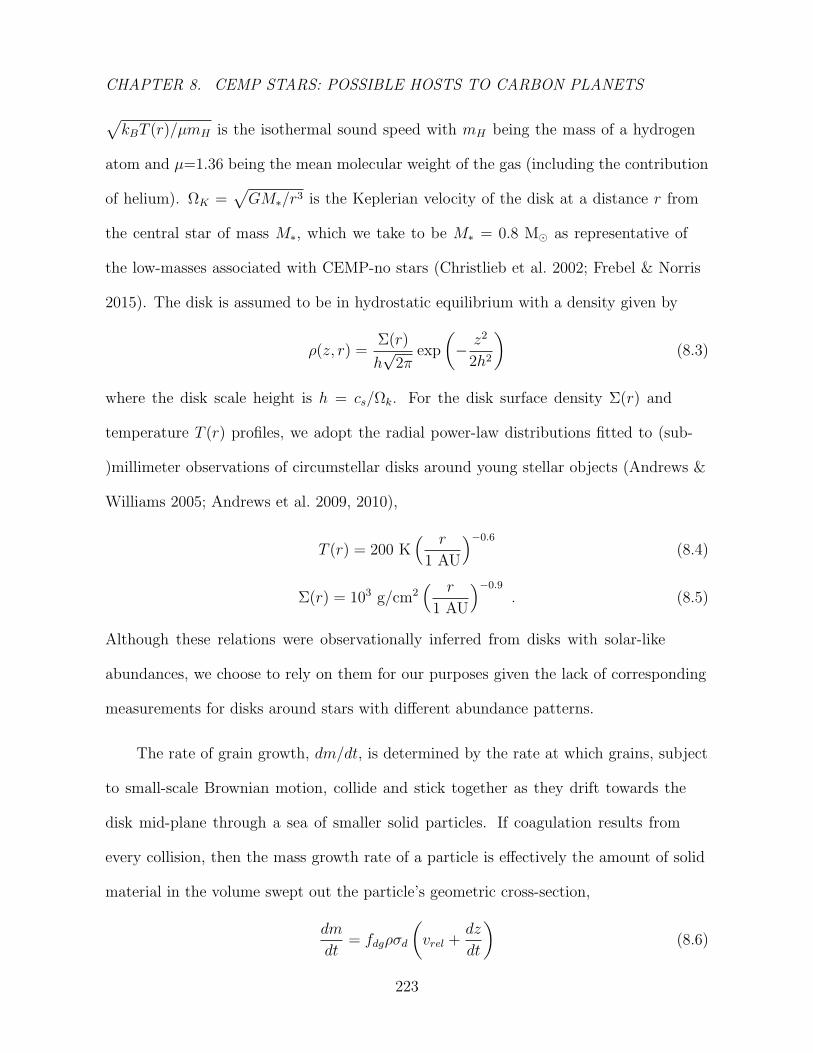
CHAPTER 8. CEMP STARS: POSSIBLE HOSTS TO CARBON PLANETS
√kBT (r)/µmH is the isothermal sound speed with mH being the mass of a hydrogen
atom and µ=1.36 being the mean molecular weight of the gas (including the contribution
of helium). ΩK =√GM∗/r3 is the Keplerian velocity of the disk at a distance r from
the central star of mass M∗, which we take to be M∗ = 0.8 M as representative of
the low-masses associated with CEMP-no stars (Christlieb et al. 2002; Frebel & Norris
2015). The disk is assumed to be in hydrostatic equilibrium with a density given by
ρ(z, r) =Σ(r)
h√
2πexp
(− z2
2h2
)(8.3)
where the disk scale height is h = cs/Ωk. For the disk surface density Σ(r) and
temperature T (r) profiles, we adopt the radial power-law distributions fitted to (sub-
)millimeter observations of circumstellar disks around young stellar objects (Andrews &
Williams 2005; Andrews et al. 2009, 2010),
T (r) = 200 K( r
1 AU
)−0.6
(8.4)
Σ(r) = 103 g/cm2( r
1 AU
)−0.9
. (8.5)
Although these relations were observationally inferred from disks with solar-like
abundances, we choose to rely on them for our purposes given the lack of corresponding
measurements for disks around stars with different abundance patterns.
The rate of grain growth, dm/dt, is determined by the rate at which grains, subject
to small-scale Brownian motion, collide and stick together as they drift towards the
disk mid-plane through a sea of smaller solid particles. If coagulation results from
every collision, then the mass growth rate of a particle is effectively the amount of solid
material in the volume swept out the particle’s geometric cross-section,
dm
dt= fdgρσd
(vrel +
dz
dt
)(8.6)
223

CHAPTER 8. CEMP STARS: POSSIBLE HOSTS TO CARBON PLANETS
where dz/dt is the dust settling velocity given by equation (2) and
vrel =
√8kBT (m1 +m2)
πm1m2
≈√
8kBT
πm(8.7)
is the relative velocity in the Brownian motion regime between grains with masses
m1 = m2 = m. To calculate the dust-to-gas mass ratio in the disk fdg, we follow the
approach in Ji et al. (2014) and relate two expressions for the mass fraction of C: (i) the
fraction of carbon in the dust, fdgMC,dust/Mdust, where Mdust is the total dust mass and
MC,dust is the carbon dust mass ; and (ii) the fraction of carbon in the gas, µCnC/µnH ,
where µC is the molecular weight of carbon (∼ 12mp) and nC and nH are the carbon and
hydrogen number densities, respectively. We then assume that a fraction fcond (referred
to from now on as the carbon condensation efficiency) of all the carbon present in the
gas cloud is locked up in dust, such that
fcondµCnCµnH
= fdgMC,dust
Mdust
. (8.8)
Since faint Population III SNe are believed to have polluted the birth clouds of CEMP-no
stars, and the only grain species that forms in non-negligible amounts in these ejecta
is amorphous carbon (Marassi et al. 2014, 2015), we set Mdust = MC,dust. Rewriting
equation (8) in terms of abundances relative to the Sun, we obtain
fdg = fcondµCµ
10[C/H]+log ε(C)−12 (8.9)
where log ε(C)=8.43±0.05 (Asplund et al. 2009) is the solar carbon abundance.
For a specified metallicity [C/H] and radial distance r from the central star, we
can then estimate the time it takes for dust grains to settle in the disk by integrating
eqs. (8.2) and (8.6) from an initial height of z(t = 0) = 4h with an initial dust grain
mass of m(t = 0) = 4πa3initρd/3. The specific weight of dust is set to ρd=2.28 g cm−3,
224

CHAPTER 8. CEMP STARS: POSSIBLE HOSTS TO CARBON PLANETS
reflecting the material density of carbon grains expected to dominate the circumstellar
disks of CEMP-no stars. The initial grain size ainit is varied between 0.01 and 1 µm to
reflect the range of characteristic radii of carbon grains found when modeling CEMP-no
star abundance patterns (Marassi et al. 2014). Comparing the resulting dust-settling
timescale to the disk lifetime given by eq. (8.1) for the specified metallicity, we can
then determine whether there is enough time for carbon dust grains to settle in the
mid-plane of the disk and there undergo runaway planetesimal formation before the disk
is dissipated by photoevaporation. For the purposes of this simple model, we neglected
possible turbulence in the disk which may counteract the effects of vertical settling,
propelling particles to higher altitudes and thus preventing them from fully settling into
the disk mid-plane (Armitage 2010). We have also not accounted for the effects of radial
drift, which may result in the evaporation of solid material in the hot inner regions of
the circumstellar disk.
As the dust settling timescale is dependent on the disk surface density Σ(r) and
temperature T (r), we find that for a given metallicity, [C/H], there is a maximum
distance rmax from the central star out to which planetesimal formation is possible. At
larger distances from the host star, the dust settling timescale exceeds the disk lifetime
and so carbon planets with semi-major axes r > rmax are not expected to form. A plot
of the maximum semi-major axis expected for planet formation around a CEMP-no star
as a function of the carbon abundance relative to the Sun [C/H] is shown in Figure 8.1
for carbon condensation efficiencies ranging between fcond = 0.1 and 1. As discovered in
Johnson & Li (2012) where the critical iron abundance for terrestrial planet formation
is considered as a function of the distance from the host star, we find a linear relation
225
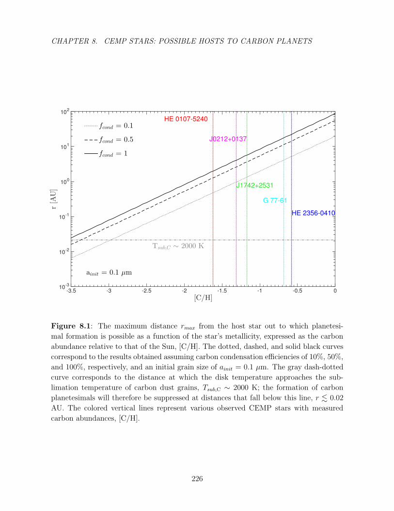
CHAPTER 8. CEMP STARS: POSSIBLE HOSTS TO CARBON PLANETS
[C/H]-3.5 -3 -2.5 -2 -1.5 -1 -0.5 0
r[A
U]
10-3
10-2
10-1
100
101
102
fcond = 0.1
fcond = 0.5
fcond = 1
HE 0107-5240
J0212+0137
J1742+2531
G 77-61
HE 2356-0410
Tsub,C ∼ 2000 K
ainit = 0.1 µm
Figure 8.1: The maximum distance rmax from the host star out to which planetesi-
mal formation is possible as a function of the star’s metallicity, expressed as the carbon
abundance relative to that of the Sun, [C/H]. The dotted, dashed, and solid black curves
correspond to the results obtained assuming carbon condensation efficiencies of 10%, 50%,
and 100%, respectively, and an initial grain size of ainit = 0.1 µm. The gray dash-dotted
curve corresponds to the distance at which the disk temperature approaches the sub-
limation temperature of carbon dust grains, Tsub,C ∼ 2000 K; the formation of carbon
planetesimals will therefore be suppressed at distances that fall below this line, r . 0.02
AU. The colored vertical lines represent various observed CEMP stars with measured
carbon abundances, [C/H].
226
CHAPTER 8. CEMP STARS: POSSIBLE HOSTS TO CARBON PLANETS
between [C/H] and rmax,
[C/H] = log( rmax
1 AU
)− α (8.10)
where α = 1.3, 1.7, and 1.9 for fcond = 0.1, 0.5, and 1, respectively, assuming an initial
grain size of ainit = 0.1 µm. These values for α change by less than 1% for smaller
initial grain sizes, ainit = 0.01 µm, and by no more than 5% for larger initial grain
sizes ainit = 1 µm; given this weak dependence on ainit, we only show our results for
a single initial grain size of ainit = 0.1 µm. The distance from the host star at which
the temperature of the disk approaches the sublimation temperature of carbon dust,
Tsub,C ∼ 2000 K (Kobayashi et al. 2011), is depicted as well (dash-dotted gray curve).
At distances closer to the central star than r ' 0.02 AU, temperatures well exceed
the sublimation temperature of carbon grains; grain growth and subsequent carbon
planetesimal formation are therefore quenched in this inner region.
Figure 8.1 shows lines representing various observed CEMP stars with measured
carbon abundances, mainly, HE 0107-5240 (Christlieb et al. 2002, 2004), SDSS
J0212+0137 (Bonifacio et al. 2015), SDSS J1742+2531 (Bonifacio et al. 2015), G 77-61
(Dahn et al. 1977; Plez & Cohen 2005; Beers et al. 2007), and HE 2356-0410 (Norris et al.
1997b; Roederer et al. 2014). These stars all have iron abundances (relative to solar)
[Fe/H] < -3.0, carbon abundances (relative to solar) [C/Fe] > 2.0, and carbon-to-oxygen
ratios C/O > 1. This latter criteria maximizes the abundance of solid carbon available
for planet formation in the circumstellar disks by optimizing carbon grain growth both
in stratified SNe ejecta and later, in the collapsing molecular birth clouds of these stars.
It also advances the possibility of carbon planet formation by ensuring that planet
formation proceeds by a carbon-rich condensation sequence in the protoplanetary disk.
SDSS J0212+0137 and HE 2356-0410 have both been classified as CEMP-no stars, with
227
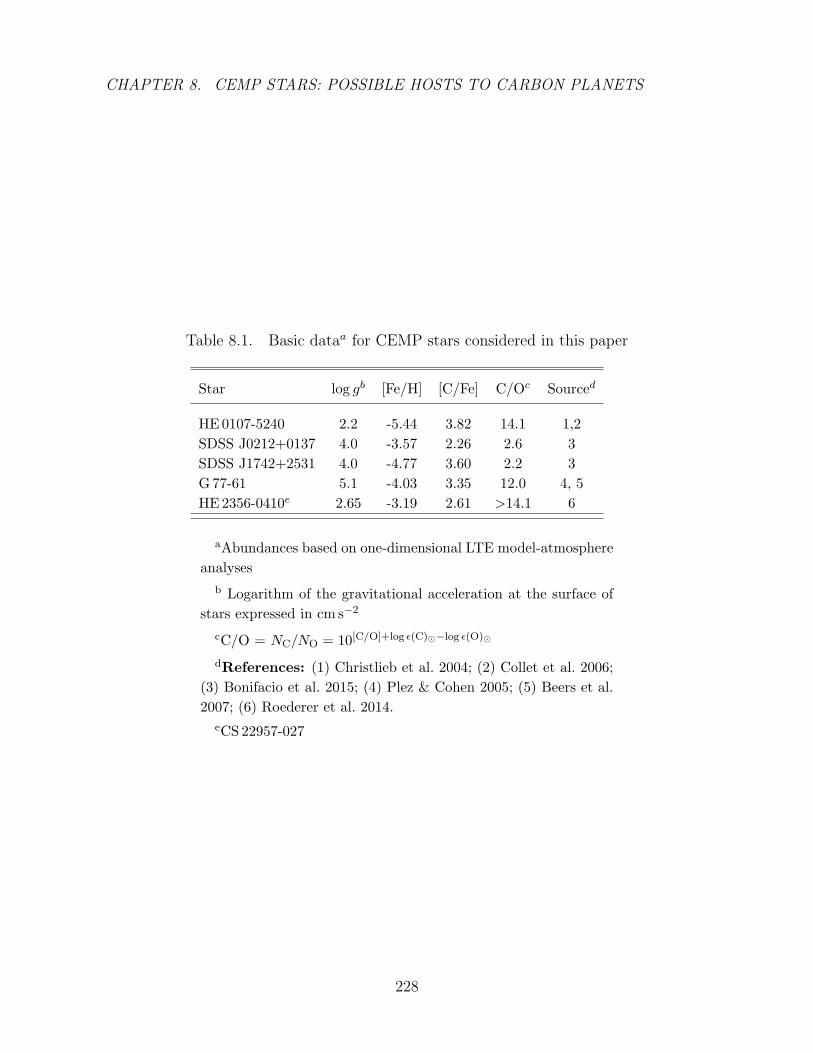
CHAPTER 8. CEMP STARS: POSSIBLE HOSTS TO CARBON PLANETS
Table 8.1. Basic dataa for CEMP stars considered in this paper
Star log gb [Fe/H] [C/Fe] C/Oc Sourced
HE 0107-5240 2.2 -5.44 3.82 14.1 1,2
SDSS J0212+0137 4.0 -3.57 2.26 2.6 3
SDSS J1742+2531 4.0 -4.77 3.60 2.2 3
G 77-61 5.1 -4.03 3.35 12.0 4, 5
HE 2356-0410e 2.65 -3.19 2.61 >14.1 6
aAbundances based on one-dimensional LTE model-atmosphere
analyses
b Logarithm of the gravitational acceleration at the surface of
stars expressed in cm s−2
cC/O = NC/NO = 10[C/O]+log ε(C)−log ε(O)
dReferences: (1) Christlieb et al. 2004; (2) Collet et al. 2006;
(3) Bonifacio et al. 2015; (4) Plez & Cohen 2005; (5) Beers et al.
2007; (6) Roederer et al. 2014.
eCS 22957-027
228
CHAPTER 8. CEMP STARS: POSSIBLE HOSTS TO CARBON PLANETS
measured barium abundances [Ba/Fe] < 0 (as defined in Beers & Christlieb 2005); the
other three stars are Ba-indeterminate, with only high upper limits on [Ba/Fe], but
are believed to belong to the CEMP-no subclass given their light-element abundance
patterns. The carbon abundance, [C/H], dominates the total metal content of the
stellar atmosphere in these five CEMP objects, contributing more than 60% of the total
metallicity in these stars. A summary of the relevant properties of the CEMP stars
considered in this analysis can be found in Table 8.1. We find that carbon planets may be
orbiting iron-deficient stars with carbon abundances [C/H] ∼ -0.6, such as HE 2356-0410,
as far out as ∼ 20 AU from their host star in the case where fcond = 1. Planets forming
around stars with less carbon enhancement, i.e. HE 0107-5240 with [C/H] ∼ -1.6, are
expected to have more compact orbits, with semi-major axes r < 2 AU. If the carbon
condensation efficiency is only 10%, the expected orbits grow even more compact, with
maximum semi-major axes of ∼ 5 and 0.5 AU, respectively.
8.5 Mass-Radius Relationship for Carbon Planets
Next we present the relationship between the mass and radius of carbon planets that we
have shown may theoretically form around CEMP-no stars. These mass-radius relations
have already been derived in the literature for a wide range of rocky and icy exoplanet
compositions (Zapolsky & Salpeter 1969; Leger et al. 2004; Valencia et al. 2006; Fortney
et al. 2007; Seager et al. 2007). Here, we follow the approach of Zapolsky & Salpeter
(1969) and solve the three canonical equations of internal structure for solid planets,
229
CHAPTER 8. CEMP STARS: POSSIBLE HOSTS TO CARBON PLANETS
1. mass conservation
dm(r)
dr= 4πr2ρ(r) , (8.11)
2. hydrostatic equilbrium
dP (r)
dr= −Gm(r)ρ(r)
r2, and (8.12)
3. the equation of state (EOS)
P (r) = f (ρ(r), T (r)) , (8.13)
where m(r) is the mass contained within radius r, P (r) is the pressure, ρ(r) is the density
of the spherical planet, and f is the unique equation of state (EOS) of the material of
interest, in this case, carbon.
Carbon grains in circumstellar disks most likely experience many shock events
during planetesimal formation which may result in the modification of their structure.
The coagulation of dust into clumps, the fragmentation of the disk into clusters of
dust clumps, the merging of these clusters into ∼ 1 km planetesimals, the collision
of planetesimals during the accretion of meteorite parent bodies, and the subsequent
collision of the parent bodies after their formation all induce strong shock waves that
are expected to chemically and physically alter the materials (Mimura & Sugisaki 2003).
Subject to these high temperatures and pressures, the amorphous carbon grains polluting
the protoplanetary disks around CEMP stars are expected to undergo graphitization and
may even crystallize into diamond (Tielens et al. 1987; Onodera et al. 1988; Papoular
et al. 1996; Takai et al. 2003). In our calculations, the equation of state at low pressures,
P ≤ 14 GPa, is set to the third-order finite strain Birch-Murnagham EOS (BME; Birch
230
CHAPTER 8. CEMP STARS: POSSIBLE HOSTS TO CARBON PLANETS
1947; Poirier 2000) for graphite,
P =3
2K0
(η7/3 − η5/3
) [1 +
3
4
(K′
0 − 4) (η2/3 − 1
)](8.14)
where η = ρ/ρ0 is the compression ratio with respect to the ambient density, ρ0, K0 is
the bulk modulus of the material, and K′0 is the pressure derivative. Empirical fits to
experimental data yields a BME EOS of graphite (ρ0 = 2.25 g cm−3) with parameters
K0 = 33.8 GPa and K′0 = 8.9 (Hanfland et al. 1989). At 14 GPa, we incorporate the
phase transition from graphite to diamond (Naka et al. 1976; Hanfland et al. 1989) and
adopt the Vinet EOS (Vinet et al. 1987, 1989),
P = 3K0η2/3(1− η−1/3
)exp
[3
2
(K′
0 − 1) (
1− η−1/3)]
(8.15)
with K0 = 444.5 GPa and K′0 = 4.18 empirically fit for diamond, ρ0 = 3.51 g cm−3
(Dewaele et al. 2008). (As pointed out in Seager et al. (2007), the BME EOS is not
fit to be extrapolated to high pressures since it is derived by expanding the elastic
potential energy as a function of pressure keeping only the lowest order terms.) Finally,
at pressures P & 1300 GPa where electron degeneracy becomes increasingly important,
we use the Thomas-Fermi-Dirac (TFD) theoretical EOS (Salpeter & Zapolsky 1967;
equations (40)-(49)), which intersects the diamond EOS at P ∼ 1300 GPa. Given that
the full temperature-dependent carbon EOSs are either undetermined or dubious at best,
all three EOSs adopted in this work are room-temperature EOSs for the sake of practical
simplification.
Using a fourth-order Runge-Kutta scheme, we solve the system of equations
simultaneously, numerically integrating eqs. (8.11) and (8.12) beginning at the planet’s
center with the inner boundary conditions M(r = 0) = 0 and P (r = 0) = Pcentral, where
Pcentral is the central pressure. The outer boundary condition P (r = Rp) = 0 then defines
231
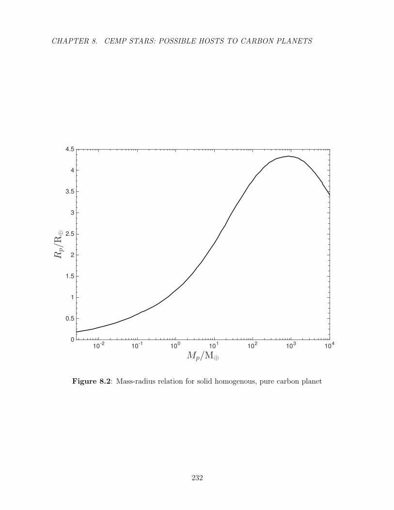
CHAPTER 8. CEMP STARS: POSSIBLE HOSTS TO CARBON PLANETS
Mp/M⊕
10-2
10-1
100
101
102
103
104
Rp/R
⊕
0
0.5
1
1.5
2
2.5
3
3.5
4
4.5
Figure 8.2: Mass-radius relation for solid homogenous, pure carbon planet
232
CHAPTER 8. CEMP STARS: POSSIBLE HOSTS TO CARBON PLANETS
the planetary radius Rp and total planetary mass Mp = m(r = Rp). Integrating these
equations for a range of Pcentral, with the appropriate EOS, P = P (ρ), to close the system
of equations, yields the mass-radius relationship for a given composition. We show this
mass-radius relation for a purely solid carbon planet in Figure 8.2. We find that for
masses Mp . 800 M⊕, gravitational forces are small compared with electrostatic Coulomb
forces in hydrostatic equilibrium and so the planet’s radius increases with increasing
mass, Rp ∝ M1/3p . However, at larger masses, the electrons are pressure-ionized and the
resulting degeneracy pressure becomes significant, causing the planet radius to become
constant and even decrease for increasing mass, Rp ∝ M−1/3p (Hubbard 1984). Planets
which fall within the mass range 500 . Mp . 1300 M⊕, where the competing effects of
Coulomb forces and electron degeneracy pressure cancel each other out, are expected
to be approximately the same size, with Rp ' 4.3 R⊕, the maximum radius of a solid
carbon planet. (In the case of gas giants, the planet radius can increase due to accretion
of hydrogen and helium.)
Although the mass-radius relation illustrated in Figure 8.2 may alone not be enough
to confidently distinguish a carbon planet from a water or silicate planet, the unique
spectral features in the atmospheres of these carbon planets may provide the needed
fingerprints. At high temperatures (T & 1000 K), the absorption spectra of massive
(M ∼ 10 - 60 M⊕) carbon planets are expected to be dominated by CO, in contrast with
the H2O-dominated spectra of hot massive planets with solar-composition atmospheres
(Kuchner & Seager 2005). The atmospheres of low-mass (M . 10 M⊕) carbon planets
are also expected to be differentiable from their solar-composition counterparts due to
their abundance of CO and CH4, and lack of oxygen-rich gases like CO2, O2, and O3
(Kuchner & Seager 2005). Furthermore, carbon planets of all masses at low temperatures
233
CHAPTER 8. CEMP STARS: POSSIBLE HOSTS TO CARBON PLANETS
are expected to accommodate hydrocarbon synthesis in their atmospheres; stable
long-chain hydrocarbons are therefore another signature feature that can help observers
distinguish the atmospheres of cold carbon planets and more confidently determine the
bulk composition of a detected planet (Kuchner & Seager 2005).
8.6 Transit Properties
The detection of theoretically proposed carbon planets around CEMP stars will provide
us with significant clues regarding how early planet formation may have started in the
Universe. While direct detection of these extrasolar planets remains difficult given the
low luminosity of most planets, techniques such as the transit method are often employed
to indirectly spot exoplanets and determine physical parameters of the planetary system.
When a planet “transits” in front of its host star, it partially occludes the star and causes
its’ observed brightness to drop by a minute amount. If the host star is observed during
one of these transits, the resulting dip in its measured light curve can yield information
regarding the relevant sizes of the star and the planet, the orbital semi-major axis, and
the orbital inclination, among other characterizing properties.
A planetary transit across a star is characterized by three main parameters: the
fractional change in the stellar brightness, the orbital period, and the duration of the
transit (Borucki et al. 1996). The fractional change in brightness is referred to as the
transit depth, ∆F (with a total observed flux F ), and is simply defined as the ratio of
the planet’s area to the host star’s area (Seager & Mallen-Ornelas 2003),
∆F =Fno transit − Ftransit
Fno transit
=
(Rp
R∗
)2
. (8.16)
234
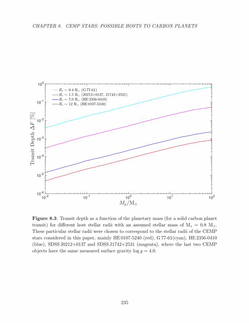
CHAPTER 8. CEMP STARS: POSSIBLE HOSTS TO CARBON PLANETS
Mp/M⊕
10-2
10-1
100
101
102
TransitDep
th∆F
[%]
10-6
10-5
10-4
10-3
10-2
10-1
100
R∗ ∼ 0.4 R⊙ (G 77-61)R∗ ∼ 1.5 R⊙ (J0212+0137, J1742+2531)R∗ ∼ 7.0 R⊙ (HE2356-0410)R∗ ∼ 12 R⊙ (HE0107-5240)
Figure 8.3: Transit depth as a function of the planetary mass (for a solid carbon planet
transit) for different host stellar radii with an assumed stellar mass of M∗ = 0.8 M.
These particular stellar radii were chosen to correspond to the stellar radii of the CEMP
stars considered in this paper, mainly HE 0107-5240 (red), G 77-61(cyan), HE 2356-0410
(blue), SDSS J0212+0137 and SDSS J1742+2531 (magenta), where the last two CEMP
objects have the same measured surface gravity log g = 4.0.
235
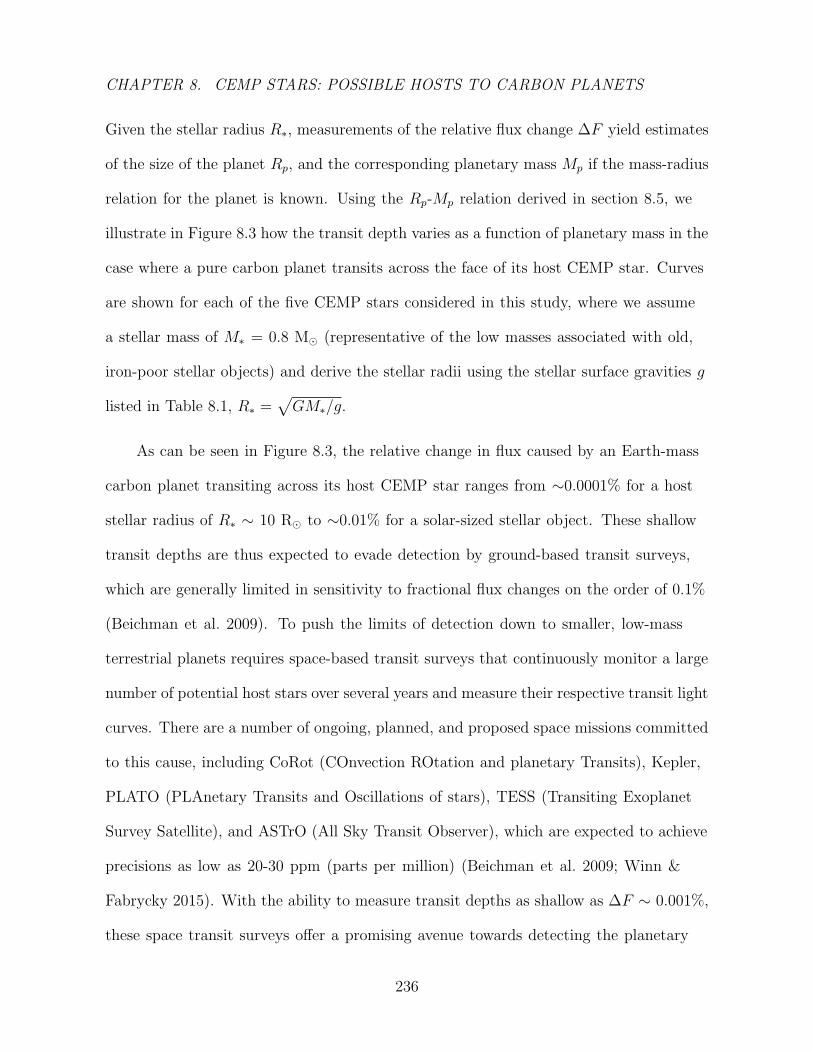
CHAPTER 8. CEMP STARS: POSSIBLE HOSTS TO CARBON PLANETS
Given the stellar radius R∗, measurements of the relative flux change ∆F yield estimates
of the size of the planet Rp, and the corresponding planetary mass Mp if the mass-radius
relation for the planet is known. Using the Rp-Mp relation derived in section 8.5, we
illustrate in Figure 8.3 how the transit depth varies as a function of planetary mass in the
case where a pure carbon planet transits across the face of its host CEMP star. Curves
are shown for each of the five CEMP stars considered in this study, where we assume
a stellar mass of M∗ = 0.8 M (representative of the low masses associated with old,
iron-poor stellar objects) and derive the stellar radii using the stellar surface gravities g
listed in Table 8.1, R∗ =√GM∗/g.
As can be seen in Figure 8.3, the relative change in flux caused by an Earth-mass
carbon planet transiting across its host CEMP star ranges from ∼0.0001% for a host
stellar radius of R∗ ∼ 10 R to ∼0.01% for a solar-sized stellar object. These shallow
transit depths are thus expected to evade detection by ground-based transit surveys,
which are generally limited in sensitivity to fractional flux changes on the order of 0.1%
(Beichman et al. 2009). To push the limits of detection down to smaller, low-mass
terrestrial planets requires space-based transit surveys that continuously monitor a large
number of potential host stars over several years and measure their respective transit light
curves. There are a number of ongoing, planned, and proposed space missions committed
to this cause, including CoRot (COnvection ROtation and planetary Transits), Kepler,
PLATO (PLAnetary Transits and Oscillations of stars), TESS (Transiting Exoplanet
Survey Satellite), and ASTrO (All Sky Transit Observer), which are expected to achieve
precisions as low as 20-30 ppm (parts per million) (Beichman et al. 2009; Winn &
Fabrycky 2015). With the ability to measure transit depths as shallow as ∆F ∼ 0.001%,
these space transit surveys offer a promising avenue towards detecting the planetary
236
CHAPTER 8. CEMP STARS: POSSIBLE HOSTS TO CARBON PLANETS
[C/H]-3.5 -3 -2.5 -2 -1.5 -1 -0.5 0
Pmax[days]
10-1
100
101
102
103
104
105
fcond = 0.1
fcond = 0.5
fcond = 1.0
HE 0107-5240
J0212+0137
J1742+2531
G 77-61
HE 2356-0410
Figure 8.4: Maximum orbital period of a carbon planet transiting across its host CEMP
star as a function of the star’s metallicity, expressed as the carbon abundance relative
to that of the Sun, [C/H]. The dotted, dashed, and solid black curves denote the results
obtained assuming carbon condensation efficiencies of 10%, 50%, and 100% in the parent
CEMP star with mass M∗ = 0.8 M. The colored vertical lines represent the five CEMP
stars considered in this paper with measured carbon abundances [C/H].
237
CHAPTER 8. CEMP STARS: POSSIBLE HOSTS TO CARBON PLANETS
systems that may have formed around CEMP stars.
The orbital period of a planet P , which can be determined if consecutive transits
are observed, is given by Kepler’s third law in the case of a circular orbit,
P 2 =4π2a3
G(M∗ +Mp)' 4π2a3
GM∗(8.17)
where a is the orbital semi-major axis and the planetary mass is assumed to be negligible
relative to the stellar mass, Mp M∗, in the second equality. Given the relation we
derived in eq. (8.10) between the metallicity [C/H] and the maximum semi-major axis
allowed for a planet orbiting a CEMP star, the maximum orbital period of the planet
can be expressed as a function of the metallicity of the host CEMP star (M∗ = 0.8 M),
Pmax ' 365.2510
32
([C/H]+α)√M∗/M
days (8.18)
where α ' 1.3, 1.7, and 1.9 for carbon condensation efficiencies of 10%, 50%, and 100%.
As can be seen in Figure 8.4, CEMP stars with higher carbon abundances [C/H], i.e.
G 77-61 and HE 2356-0410, and larger efficiencies for carbon dust condensation fcond, can
host planets with wider orbits and slower rotations, resulting in transits as infrequently
as once every couple hundred years. Conversely, carbon planets orbiting relatively less
carbon-rich CEMP stars, like SDSS J0212+0137, are expected to have higher rates of
transit reoccurrence, completing rotations around their parent stars every ∼ 1-10 years.
These shorter period planets therefore have a much higher probability of producing an
observable transit.
The maximum duration of the transit, T , can also be expressed as a function of the
metallicity [C/H] of the parent CEMP star. For transits across the center of a star, the
total duration is given by,
T ' 2R∗
√a
GM∗(8.19)
238
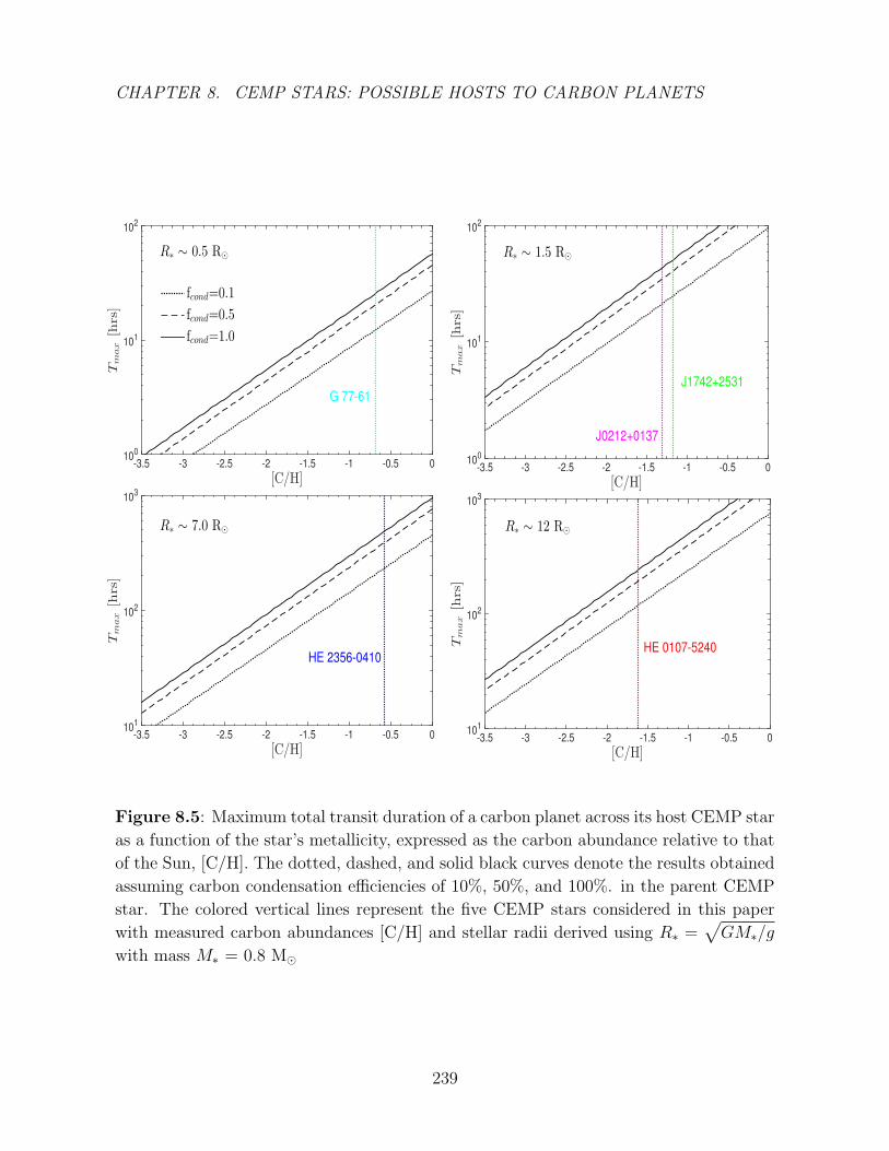
CHAPTER 8. CEMP STARS: POSSIBLE HOSTS TO CARBON PLANETS
[C/H]-3.5 -3 -2.5 -2 -1.5 -1 -0.5 0
Tmax[hrs]
100
101
102
fcond=0.1
fcond=0.5
fcond=1.0
[C/H]-3.5 -3 -2.5 -2 -1.5 -1 -0.5 0
Tmax[hrs]
100
101
102
[C/H]-3.5 -3 -2.5 -2 -1.5 -1 -0.5 0
Tmax[hrs]
101
102
103
[C/H]-3.5 -3 -2.5 -2 -1.5 -1 -0.5 0
Tmax[hrs]
101
102
103
R∗ ∼ 7.0 R⊙
R∗ ∼ 0.5 R⊙
HE 2356-0410
G 77-61
R∗ ∼ 1.5 R⊙
J1742+2531
J0212+0137
HE 0107-5240
R∗ ∼ 12 R⊙
Figure 8.5: Maximum total transit duration of a carbon planet across its host CEMP star
as a function of the star’s metallicity, expressed as the carbon abundance relative to that
of the Sun, [C/H]. The dotted, dashed, and solid black curves denote the results obtained
assuming carbon condensation efficiencies of 10%, 50%, and 100%. in the parent CEMP
star. The colored vertical lines represent the five CEMP stars considered in this paper
with measured carbon abundances [C/H] and stellar radii derived using R∗ =√GM∗/g
with mass M∗ = 0.8 M
239
CHAPTER 8. CEMP STARS: POSSIBLE HOSTS TO CARBON PLANETS
with the assumption that Mp M∗ and Rp R∗. Once again, using the relation from
eq. (8.10) to express the maximum orbital distance from the host star in terms of the
star’s carbon abundance, we find that the maximum transit duration of a carbon planet
across its parent CEMP star (M∗ = 0.8 M) is
Tmax ' 13R∗R
√10[C/H]+α
M∗/Mhrs . (8.20)
In Figure 8.5, these maximum durations are shown as a function of [C/H] for the various
stellar radii associated with the CEMP stars we consider in this paper. Transits across
CEMP stars with larger radii and higher carbon abundances are expected to take much
longer. While the total transit duration across SDSS J0212+0137 and SDSS J1742+2531
with R∗ ∼ 1.5 R and metallicities of [C/H] ∼ -1.3 – -1.2, is at most ∼ 1-2 days,
transits across HE 0107-5240 (R∗ ∼ 12 R, [C/H]∼ -1.6) can take up to 2 weeks (fcond =
1). In general, the geometric probability of a planet passing between the observer and
the planet’s parent star increases with stellar radius and decreases with orbital radius,
pt ' R∗/a Kane (2007). Therefore, focusing on CEMP stars, such as HE 0107-5240 and
HE 2356-0410, with large stellar radii increases the observer’s chance of spotting transits
and detecting a planetary system.
8.7 Discussion
We explored in this paper the possibility of carbon planet formation around the
iron-deficient, carbon-rich subset of low-mass stars known as CEMP stars. The observed
abundance patterns of CEMP-no stars suggest that these stellar objects were probably
born out of gas enriched by massive first-generation stars that ended their lives as
Type II SNe with low levels of mixing and a high degree of fallback. The formation of
240
CHAPTER 8. CEMP STARS: POSSIBLE HOSTS TO CARBON PLANETS
dust grains in the ejecta of these primordial core-collapsing SNe progenitors has been
observationally confirmed and theoretically studied. In particular, amorphous carbon
is the only grain species found to condense and form in non-negligible amounts in SN
explosion models that are tailored to reproduce the abundance patterns measured in
CEMP-no stars. Under such circumstances, the gas clouds which collapse and fragment
to form CEMP-no stars and their protoplanetary disks may contain significant amounts
of carbon dust grains imported from SNe ejecta. The enrichment of solid carbon in the
protoplanetary disks of CEMP stars may then be further enhanced by Fischer-Trope-type
reactions and carbon-rich condensation sequences, where the latter occurs specifically in
nebular gas with C/O & 1.
For a given metallicity [C/H] of the host CEMP star, the maximum distance out
to which planetesimal formation is possible can then be determined by comparing the
dust-settling timescale in the protostellar disk to the expected disk lifetime. Assuming
that disk dissipation is driven by a metallicity-dependent photoevaporation rate, we
find a linear relation between [C/H] and the maximum semi-major axis of a carbon
planet orbiting its host CEMP star. Very carbon-rich CEMP stars, such as G 77-61 and
HE 2356-0410 with [C/H] ' -0.7 – -0.6, can host carbon planets with semi-major axes as
large ∼ 20 AU for 100% carbon condensation efficiencies; this maximum orbital distance
reduces to ∼ 5 AU when the condensation efficiency drops by an order of magnitude.
In the case of the observed CEMP-no stars HE 0107-5240, SDSS J0212+0137, and
SDSS J1742+2531, where the carbon abundances are in the range [C/H] ' -1.6 – -1.2,
we expect more compact orbits, with maximum orbital distances rmax ' 2, 4, and 6 AU,
respectively, for fcond = 1 and rmax ' 0.5 - 1 AU for fcond = 0.1.
We then use the linear relation found between [C/H] and rmax (section 8.4), along
241
CHAPTER 8. CEMP STARS: POSSIBLE HOSTS TO CARBON PLANETS
with the theoretical mass-radius relation derived for a solid, pure carbon planet (section
8.5), to compute the three observable characteristics of planetary transits: the orbital
period, the transit depth, and the transit duration. We find that the relative change in
flux, ∆F , caused by an Earth-mass carbon planet transiting across its host CEMP star
ranges from ∼ 0.0001% for a stellar radius of R∗ ∼ 10 R to ∼ 0.01% for a solar-sized
stellar host. While the shallow transit depths of Earth-mass carbon planets around
HE 0107-5240 and HE 2356-0410 may evade detection, current and future space-based
transit surveys promise to achieve the precision levels (∆F ∼ 0.001%) necessary to detect
planetary systems around CEMP stars such as SDSS J0212+0137, SDSS J1742+2531,
and G 77-61.
Short orbital periods and long transit durations are also key ingredients in boosting
the probability of transit detection by observers. G 77-61 is not an optimal candidate
in these respects since given its large carbon abundance ([C/Fe] ∼ 3.4), carbon planets
may form out to very large distances and take up to a century to complete an orbit
around the star for fcond = 1 (Pmax ∼ 10 years for 10% carbon condensation efficiency).
The small stellar radius, R∗ ∼ 0.5 R, also reduces chances of spotting the transit since
the resulting transit duration is only ∼ 30 hours at most. Carbon planets around larger
CEMP stars with an equally carbon-rich protoplanetary disk, such as HE 2356-0410
(R∗ ∼ 7 R), have a better chance of being spotted, with transit durations lasting up to
∼ 3 weeks. The CEMP-stars SDSS J0212+0137, and SDSS J1742+2531 are expected to
host carbon planets with much shorter orbits, Pmax ∼ 16 years for 100% condensation
efficiency (Pmax ∼ 1 year for fcond = 0.1), and transit durations that last as long as ∼
60 hours. If the ability to measure transit depths improves to a precision of 1 ppm, then
potential carbon planets around HE 0107-5240 are the most likely to be spotted (among
242
CHAPTER 8. CEMP STARS: POSSIBLE HOSTS TO CARBON PLANETS
the group of CEMP-no stars considered in this paper), transiting across the host star at
least once every ∼ 5 months (10% condensation efficiency) with a transit duration of 6
days.
While our calculations place upper bounds on the distance from the host star
out to which carbon planets can form, we note that orbital migration may alter
a planet’s location in the circumstellar disk. As implied by the existence of ‘hot
Jupiters’, it is possible for a protoplanet that forms at radius r to migrate inward either
through gravitational interactions with other protoplanets, resonant interactions with
planetesimals with more compact orbits, or tidal interactions with gas in the surrounding
disk (Papaloizou & Terquem 2006). Since Figure 8.1 only plots rmax, the maximum
distance out to which a carbon planet with [C/H] can form, our results remain consistent
in the case of an inward migration. However, unless planets migrate inward from their
place of birth in the disk, we do not expect to find carbon exoplanets orbiting closer
than r ' 0.02 AU from the host stars since at such close proximities, temperatures are
high enough to sublimate carbon dust grains.
Protoplanets can also be gravitationally scattered into wider orbits through
interactions with planetesimals in the disk(Hahn & Malhotra 1999; Veras et al. 2009).
Such an outward migration of carbon planets may result in observations that are
inconsistent with the curves in Figure 8.1. A planet that formed at radius r rmax
still has room to migrate outwards without violating the ‘maximum distance’ depicted
in Figure 8.1; however, the outward migration of a carbon planet that originally formed
at, or near, rmax would result in a breach of the upper bounds placed on the transiting
properties of carbon planets (section 8.6). In particular, a carbon planet that migrates
to a semi-major axis r > rmax will have an orbital period and a transit duration time
243
CHAPTER 8. CEMP STARS: POSSIBLE HOSTS TO CARBON PLANETS
that exceeds the limits prescribed in eqs. (8.18) and (8.20), respectively.
Detection of the carbon planets that we suggest may have formed around CEMP
stars will provide us with significant clues regarding how planet formation may have
started in the early Universe. The formation of planetary systems not only signifies an
increasing degree of complexity in the young Universe, but it also carries implications
for the development of life at this early junction (Loeb 2014). The lowest metallicity
planetary system detected to date is around BD+20 24 57, a K2-giant with [Fe/H] =
-1.0 (Niedzielski et al. 2009), a metallicity already well below the critical value once
believed to be necessary for planet formation (Gonzalez et al. 2001; Pinotti et al. 2005).
More recent formulations of the minimum metallicity required for planet formation are
consistent with this observation, estimating that the first Earth-like planets likely formed
around stars with metallicities [Fe/H] . -1.0 (Johnson & Li 2012). The CEMP stars
considered in this paper are extremely iron-deficient, with [Fe/H] . -3.2, and yet, given
the enhanced carbon abundances which dominate the total metal content in these stars
( [C/H] & -1.6), the formation of solid carbon exoplanets in the protoplanetary disks of
CEMP stars remains a real possibility. An observational program aimed at searching
for carbon planets around these low-mass Population II stars could therefore potentially
shed light on the question of how early planets, and subsequently, life could have formed
after the Big Bang.
8.8 Acknowledgments
We are thankful to Sean Andrews and Karin Oberg for helpful discussions and feedback.
This work was supported in part by NSF grant AST-1312034. This material is
244

CHAPTER 8. CEMP STARS: POSSIBLE HOSTS TO CARBON PLANETS
based upon work supported by the National Science Foundation Graduate Research
Fellowship under Grant No. DGE1144152. Any opinion, findings, and conclusions
or recommendations expressed in this material are those of the authors and do not
necessarily reflect the views of the National Science Foundation.
245
Chapter 9
EPILOGUE
The Darkest of All Ends: Hunting
Black Holes with GAIA
This thesis chapter has been submitted to Monthly Notices of the Royal
Astronomical Society, and originally appeared in the arXiv as
N. Mashian and A. Loeb, Hunting Black Holes with GAIA,
2017
9.1 Abstract
We predict the number of black holes with stellar companions that are potentially
detectable with GAIA astrometry over the course of its five-year mission. Our model
estimates that nearly 3×10⁵ astrometric binaries hosting black holes and stellar
246

CHAPTER 9. HUNTING BLACK HOLES WITH GAIA
companions brighter than GAIA’s detection threshold, G ∼ 20, should be discovered
with 5σ sensitivity. Among these detectable binaries, systems with longer orbital periods
are favored, and black hole and stellar companion masses in the range MBH ∼ 6 - 10 M
and M∗ ∼ 1 - 2 M, respectively, are expected to dominate.
9.2 Introduction
Stellar evolution models, chemical enrichment by supernovae within the Milky Way,
and gravitational microlensing events all indicate that a population of about ∼108-109
stellar-mass black holes resides in our Galaxy (Shapiro & Teukolsky 1983; van den
Heuvel 1992; Brown & Bethe 1994; Samland 1998; Agol et al. 2002). And yet, despite
such high estimates, fewer than fifty stellar black hole candidates have been studied and
confirmed, all of which are in X-ray binary systems (G. & van der Klis M. 2006; Casares
2007; Fender et al. 2013; Narayan & McClintock 2013). We are therefore left to wonder,
where are all these “missing” black holes and how can we observe them?
While black holes in binary systems with ongoing mass transfer have been
preferentially detected via X-rays, we expect that at any given moment, a dominant
fraction of stellar black holes reside in binaries with no substantial X-ray emission. The
binary system may be an X-ray transient, undergoing dramatic episodes of enhanced
mass-transfer followed by quiescent phases where the X-rays switch off and the flux
drops by several magnitudes; all known low mass black hole binaries (LMBHBs) fall into
this category, demonstrating transient behavior (Tanaka & Lewin 1995; White et al.
1995; J. & R. 2006). Menou et al. (1999) suggested that there may be a population of
persistent LMBHBs that are simply dim due to the very low radiative efficiencies of their
247
CHAPTER 9. HUNTING BLACK HOLES WITH GAIA
advection-dominated accretion flow zones. These systems lack large-amplitude outbursts
and thus remain difficult to detect with their persistent, yet faint X-ray emission.
There may be a significant number of stellar black holes residing in detached binary
systems with companion stars that have not yet reached, or may never reach, the
evolutionary stage of transferring mass by Roche-lobe overflow to their compact primaries
(Yungelson et al. 2006). Karpov & Lipunov (2001) suggests the existence of hundreds
of times more detached binaries composed of a massive OB star and a stellar-wind
accreting black hole that remain impossible to detect through X-ray observations. The
spherically symmetric accretion that takes place in these systems can only result in the
effective generation of a hard radiation component if equipartition is established between
the gravitational and magnetic energies in the flow. Given the magnetic exhaust effect
operating in these binaries, such equilibrium is rarely established and most black holes
in these systems remain unobservable (Karpov & Lipunov 2001).
Given the difficulties associated with detecting stellar-mass black holes in binary
systems with no substantial X-ray emission, we explore the possibility of discovering
these elusive, compact objects through astrometric observations. The recent advent
of the European Space Agency mission Gaia (Perryman et al. 2001) is expected to
transform the field of astrometry by measuring the three-dimensional spatial and velocity
distribution of nearly ∼ 1 billion stars brighter than magnitude G ∼ 20 (Lindegren et al.
2016). Over the course of its five-year mission lifetime, Gaia is expected to perform an
all-sky survey, observing each source an average of 70 times and yielding final astrometric
accuracies of roughly 10 µas (micro-arcsec) between G ∼ 6 - 12, 25 µas at G ∼ 15, and
300 µas at G ∼ 20 (Gaia Collaboration et al. 2016). By surveying an unprecedented
1% of the Galaxy’s total stellar population with unparalleled precision, Gaia will not
248
CHAPTER 9. HUNTING BLACK HOLES WITH GAIA
only confirm and improve upon observations of the few dozen active X-ray binaries that
have already been closely studied, but it will also provide a unique opportunity to detect
astrometric binaries that have one invisible component, i.e. a black hole, by observing
the motion of the visible companion around the system’s barycenter.
In this Letter, we seek to estimate the number of black holes with stellar companions
that are potentially detectable with Gaia astrometry. We outline the components of our
model and explore the various constraints on the detectability of these binary systems
in section 9.3. Our results are presented and discussed in section 9.4. We adopt a flat,
ΛCDM cosmology with Ωm = 0.3, ΩΛ = 0.7, and H0 = 70 km s−1Mpc−1, consistent with
the most recent measurements from the Planck satellite (Planck Collaboration et al.
2016b).
9.3 The Model
To calculate the number of black holes we expect Gaia to detect astrometrically over
its five-year lifetime, our model accounts for several limiting factors: (i) the fraction of
stars assumed to end their lives as a black hole in a binary system with a fellow stellar
companion; (ii) the fraction of those systems with stellar companions that are still
shining and whose astrometric wobbles are thus detectable; (iii) the fraction of those
systems with periods in the range that Gaia can observe given its mission lifetime and
astrometric precision; and (iv) the volume of space Gaia can probe given its detection
threshold of G ∼ 20. We will now briefly discuss each factor in turn.
249
CHAPTER 9. HUNTING BLACK HOLES WITH GAIA
9.3.1 Black holes with stellar companions
The massive star progenitors of stellar black holes are commonly found in binaries, with
galactic surveys yielding bias-corrected spectroscopic binary fractions of 0.6-0.7 in the
Milky Way (Kobulnicky & Fryer 2007; Sana et al. 2012; Dunstall et al. 2015; Sana 2017).
Kiminki & Kobulnicky (2012) suggest that the binary fraction among these massive stars
may even be as high as 90% for systems with periods up to 104 years. The question then
becomes whether these black hole progenitors keep their companions throughout the
stellar evolutionary process. Various phenomena can lead to the unbinding of a binary,
including dynamical interactions, mass loss, supernova explosions of either companion,
and merging of the two sources. Fender et al. (2013) estimate that about one quarter
of O-stars merge with their companions during evolution and that nearly 50% of black
holes have companions that undergo iron core-collapse supernovae (CCSNe), producing
neutron stars with natal kicks that can unbind the system with their large velocities.
The formation of the black hole itself may disturb the binary system depending on
the formation mechanism. For the lower mass end of black hole progenitors, a metastable
proto-neutron star (PNS) is left behind by a weak CCSN and a black hole appears after
fallback accretion of the part of the stellar envelope that was not successfully expelled by
the supernova (SN) explosion. In the case of more massive stars with larger iron cores,
successful SNe explosions are even more difficult to achieve and black holes are formed
through accretion of the entire stellar material, either through direct collapse or as a
result of failed SNe (Kochanek et al. 2008; Belczynski et al. 2010; Adams et al. 2016).
This notion that some massive stars undergo collapse without producing an explosion
was first invoked by theorists to explain away difficulties in producing SN explosions in
250
CHAPTER 9. HUNTING BLACK HOLES WITH GAIA
analytical models and hydrodynamic simulations (Woosley & Weaver 1986; Gould &
Salim 2002). Since then, failed SNe have gained ground as a possible mechanism for
producing cosmological gamma-ray bursts (Woosley 1993) and as a potential solution
to the “Red Supergiant Problem”, referring to the statistically significant absence of
higher mass (& 16 M) red supergiants exploding as SNe (Smartt 2009, 2015). Evidence
in line with the suggestion that & 16 M stars do not explode as optically bright SNe
has been mounting in recent years. To date, there have been no observed Type IIP SNe
with strong [OII] emission consistent with a zero-age main sequence (ZAMS) progenitor
mass & 16 M (Jerkstrand et al. 2014). Furthermore, Brown & Woosley (2013) found
that Galactic abundances can be reproduced even if no stars with masses above 25
M contribute metals via SN explosions, a mass threshold that can be even lower if
uncertain mass loss parameters and reaction rates are modified. Though simulations
suggest that there is no single mass below which all stars explode and above which black
holes form by implosion, typically 95% of stars that do explode have masses less than 20
M (Sukhbold et al. 2016). For those stars that end up as black holes, which are most
but not all stars with masses above 20 M, only a few were found to form black holes
via fallback (Sukhbold et al. 2016).
Given the theoretical predictions and supporting observations, we assume for the
purposes of our calculation that progenitor stars with mass ≥ 20 M will collapse
to form black holes without undergoing an explosion. The mass loss experienced by
these black hole progenitors may effectively disrupt the binary if the system loses more
than half of its mass suddenly during stellar collapse; in such cases, the newly formed
black hole may receive a natal kick, enhancing binary disruption (Repetto et al. 2012;
Lovegrove & Woosley 2013; Kochanek 2015). On the other hand, if the progenitor loses
251
CHAPTER 9. HUNTING BLACK HOLES WITH GAIA
its mass gradually, i.e. via wind, adiabatic invariants should be preserved and the binary
separation will adjust accordingly to accommodate the mass loss, allowing the binary to
remain gravitationally bound (Smith 2014). The final fraction of stellar objects assumed
to end their lives as a black hole in a binary system is thus,
fB.F. = f
∫ 150 M
20 M
ε(M∗)dM∗ , (9.1)
where f is fudge factor accounting for the fraction of black hole progenitor stars that
either never host a companion, or lose their companion over the course of stellar
evolution. Rapid mass loss and SN-like kicks during black hole formation will result in
small values of f , while formation via implosion or failed SN of stripped Wolf-Rayet stars
imply values closer to unity.
The initial mass function (IMF) of progenitor stars, ε(M∗), is a multi-part power
law taken from Kroupa (2007),
ε(M∗) = k
(M∗0.5
)−1.30.1 < M∗ ≤ 0.5 M(
M∗0.5
)−2.30.5 < M∗ ≤ 150 M
where k is set to normalize the distribution such that∫ 150 M
0.1 MdM∗ε(M∗) = 1.
9.3.2 Visible binary companions
In order to detect a black hole via the astrometric wobble of its stellar companion, the
star must still be shining, i.e. observable in the visual range. To determine the fraction
of binary systems with stellar sources that are currently burning fuel, we adopt the
simplifying assumption that the Milky Way stars follow the cumulative star-formation
252
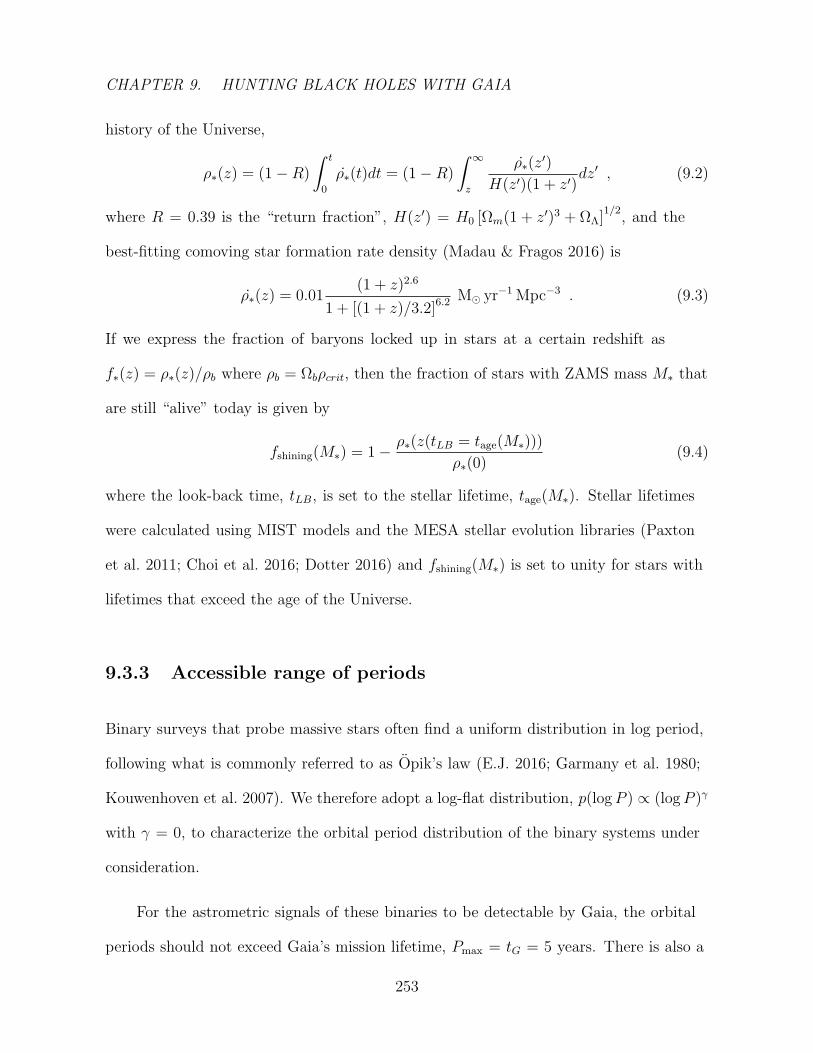
CHAPTER 9. HUNTING BLACK HOLES WITH GAIA
history of the Universe,
ρ∗(z) = (1−R)
∫ t
0
ρ∗(t)dt = (1−R)
∫ ∞z
ρ∗(z′)
H(z′)(1 + z′)dz′ , (9.2)
where R = 0.39 is the “return fraction”, H(z′) = H0 [Ωm(1 + z′)3 + ΩΛ]1/2
, and the
best-fitting comoving star formation rate density (Madau & Fragos 2016) is
ρ∗(z) = 0.01(1 + z)2.6
1 + [(1 + z)/3.2]6.2M yr−1 Mpc−3 . (9.3)
If we express the fraction of baryons locked up in stars at a certain redshift as
f∗(z) = ρ∗(z)/ρb where ρb = Ωbρcrit, then the fraction of stars with ZAMS mass M∗ that
are still “alive” today is given by
fshining(M∗) = 1− ρ∗(z(tLB = tage(M∗)))
ρ∗(0)(9.4)
where the look-back time, tLB, is set to the stellar lifetime, tage(M∗). Stellar lifetimes
were calculated using MIST models and the MESA stellar evolution libraries (Paxton
et al. 2011; Choi et al. 2016; Dotter 2016) and fshining(M∗) is set to unity for stars with
lifetimes that exceed the age of the Universe.
9.3.3 Accessible range of periods
Binary surveys that probe massive stars often find a uniform distribution in log period,
following what is commonly referred to as Opik’s law (E.J. 2016; Garmany et al. 1980;
Kouwenhoven et al. 2007). We therefore adopt a log-flat distribution, p(logP ) ∝ (logP )γ
with γ = 0, to characterize the orbital period distribution of the binary systems under
consideration.
For the astrometric signals of these binaries to be detectable by Gaia, the orbital
periods should not exceed Gaia’s mission lifetime, Pmax = tG = 5 years. There is also a
253
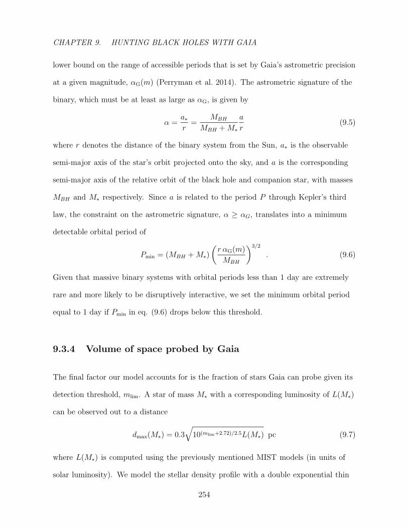
CHAPTER 9. HUNTING BLACK HOLES WITH GAIA
lower bound on the range of accessible periods that is set by Gaia’s astrometric precision
at a given magnitude, αG(m) (Perryman et al. 2014). The astrometric signature of the
binary, which must be at least as large as αG, is given by
α =a∗r
=MBH
MBH +M∗
a
r(9.5)
where r denotes the distance of the binary system from the Sun, a∗ is the observable
semi-major axis of the star’s orbit projected onto the sky, and a is the corresponding
semi-major axis of the relative orbit of the black hole and companion star, with masses
MBH and M∗ respectively. Since a is related to the period P through Kepler’s third
law, the constraint on the astrometric signature, α ≥ αG, translates into a minimum
detectable orbital period of
Pmin = (MBH +M∗)
(r αG(m)
MBH
)3/2
. (9.6)
Given that massive binary systems with orbital periods less than 1 day are extremely
rare and more likely to be disruptively interactive, we set the minimum orbital period
equal to 1 day if Pmin in eq. (9.6) drops below this threshold.
9.3.4 Volume of space probed by Gaia
The final factor our model accounts for is the fraction of stars Gaia can probe given its
detection threshold, mlim. A star of mass M∗ with a corresponding luminosity of L(M∗)
can be observed out to a distance
dmax(M∗) = 0.3√
10(mlim+2.72)/2.5L(M∗) pc (9.7)
where L(M∗) is computed using the previously mentioned MIST models (in units of
solar luminosity). We model the stellar density profile with a double exponential thin
254

CHAPTER 9. HUNTING BLACK HOLES WITH GAIA
and thick disk centered at the solar position in the Galaxy, (R, Z) = (8 kpc, 25 pc),
with scale lengths of hR,thin = 2.6 kpc and hR,thick = 3.6 kpc, scale heights of hz,thin = 0.3
kpc and hR,thick = 0.9 kpc, and a normalization of the thick disk (relative to the thin) of
fthick = 0.04 (Juric et al. 2008; Yoshii 2013). Normalized further to yield a total stellar
mass of M∗,tot = 6.08×10¹⁰ M (Licquia & Newman 2015), this stellar number density
distribution takes the following form (in spherical coordinates),
n(r, θ, φ) = n0
[exp
(−(r sinφ+R)
2.6 kpc− |r cosφ+ Z|
0.3 kpc
)+ 0.04 exp
(−(r sinφ+R)
3.6 kpc− |r cosφ+ Z|
0.9 kpc
)] (9.8)
where n0 ≈ 3 pc−3.
Taking into account all these various limiting factors, the resulting total number of
black holes we can expect Gaia to observe astrometrically over the course of its five-year
mission takes the following form,
Ntot = fB.F.
∫ ∞5 M
dMBH ψ(MBH)
∫ 150 M
0.1 M
dM∗ fshining(M∗) ε(M∗)
∫ 2π
0
dθ
∫ π
0
dφ sinφ ×∫ dmax(M∗,mlim)
0
dr r2
∫ log (tG)
log (Max[1 day, Pmin(r,M∗,MBH)])
d (logP ) n(r, θ, φ) p (logP ) ,
(9.9)
where ψ(MBH) represents the black hole mass distribution adopted from Ozel et al.
(2010, 2012),
ψ(MBH) =A(MBH)δ +
[B(MBH)−δ + C(MBH)−δ
]−11/δ
, (9.10)
with δ = -10.0 and,
A(MBH) = 4.367− 1.7294MBH + 0.1713M2BH
B(MBH) = 14.24e−0.542MBH
C(MBH) = 3.322e−0.386MBH . (9.11)
255
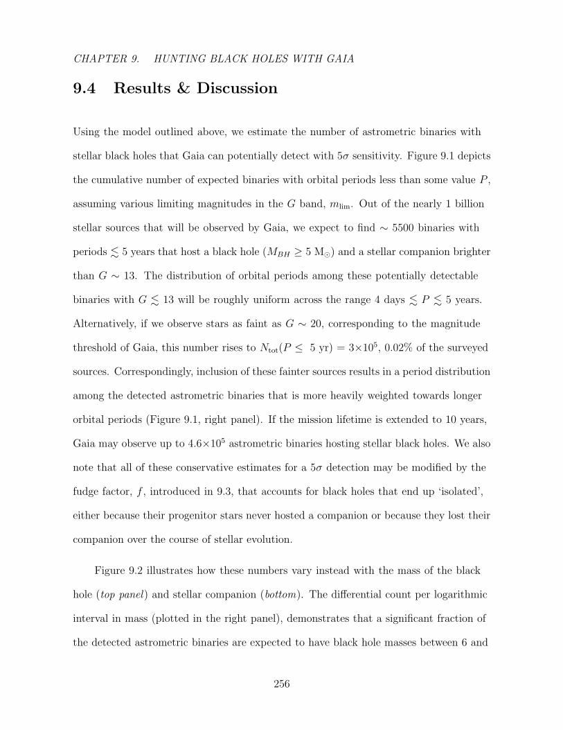
CHAPTER 9. HUNTING BLACK HOLES WITH GAIA
9.4 Results & Discussion
Using the model outlined above, we estimate the number of astrometric binaries with
stellar black holes that Gaia can potentially detect with 5σ sensitivity. Figure 9.1 depicts
the cumulative number of expected binaries with orbital periods less than some value P ,
assuming various limiting magnitudes in the G band, mlim. Out of the nearly 1 billion
stellar sources that will be observed by Gaia, we expect to find ∼ 5500 binaries with
periods . 5 years that host a black hole (MBH ≥ 5 M) and a stellar companion brighter
than G ∼ 13. The distribution of orbital periods among these potentially detectable
binaries with G . 13 will be roughly uniform across the range 4 days . P . 5 years.
Alternatively, if we observe stars as faint as G ∼ 20, corresponding to the magnitude
threshold of Gaia, this number rises to Ntot(P ≤ 5 yr) = 3×10⁵, 0.02% of the surveyed
sources. Correspondingly, inclusion of these fainter sources results in a period distribution
among the detected astrometric binaries that is more heavily weighted towards longer
orbital periods (Figure 9.1, right panel). If the mission lifetime is extended to 10 years,
Gaia may observe up to 4.6×10⁵ astrometric binaries hosting stellar black holes. We also
note that all of these conservative estimates for a 5σ detection may be modified by the
fudge factor, f , introduced in 9.3, that accounts for black holes that end up ‘isolated’,
either because their progenitor stars never hosted a companion or because they lost their
companion over the course of stellar evolution.
Figure 9.2 illustrates how these numbers vary instead with the mass of the black
hole (top panel) and stellar companion (bottom). The differential count per logarithmic
interval in mass (plotted in the right panel), demonstrates that a significant fraction of
the detected astrometric binaries are expected to have black hole masses between 6 and
256

CHAPTER 9. HUNTING BLACK HOLES WITH GAIA
P [yr]10-2 10-1 100
f−1Ntot(≤
P)
101
102
103
104
105
106mlim = 13mlim = 15mlim = 20
P [yr]10-2 10-1 100
f−1dNtot/dlnP
102
103
104
105
106
Figure 9.1: Left panel : Cumulative number of detectable astrometric binaries hosting
black holes with orbital periods less than P , assuming detection thresholds of mlim =
13, 15, and 20 in the G band. Right panel : The corresponding differential count per
logarithmic interval in P . Numbers are shown for a 5σ detection and may be modified
by a multiplicative factor f to account for the fraction of black hole progenitor stars that
end their lives isolated.
257
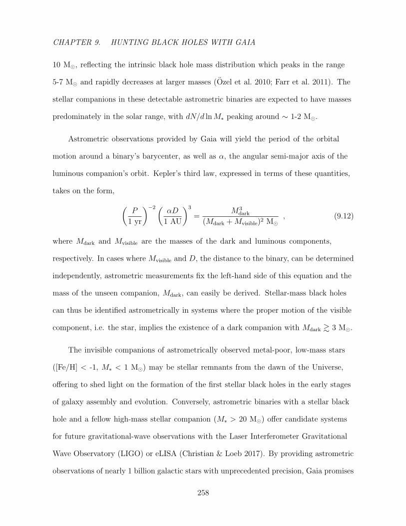
CHAPTER 9. HUNTING BLACK HOLES WITH GAIA
10 M, reflecting the intrinsic black hole mass distribution which peaks in the range
5-7 M and rapidly decreases at larger masses (Ozel et al. 2010; Farr et al. 2011). The
stellar companions in these detectable astrometric binaries are expected to have masses
predominately in the solar range, with dN/d lnM∗ peaking around ∼ 1-2 M.
Astrometric observations provided by Gaia will yield the period of the orbital
motion around a binary’s barycenter, as well as α, the angular semi-major axis of the
luminous companion’s orbit. Kepler’s third law, expressed in terms of these quantities,
takes on the form, (P
1 yr
)−2(αD
1 AU
)3
=M3
dark
(Mdark +Mvisible)2 M, (9.12)
where Mdark and Mvisible are the masses of the dark and luminous components,
respectively. In cases where Mvisible and D, the distance to the binary, can be determined
independently, astrometric measurements fix the left-hand side of this equation and the
mass of the unseen companion, Mdark, can easily be derived. Stellar-mass black holes
can thus be identified astrometrically in systems where the proper motion of the visible
component, i.e. the star, implies the existence of a dark companion with Mdark & 3 M.
The invisible companions of astrometrically observed metal-poor, low-mass stars
([Fe/H] < -1, M∗ < 1 M) may be stellar remnants from the dawn of the Universe,
offering to shed light on the formation of the first stellar black holes in the early stages
of galaxy assembly and evolution. Conversely, astrometric binaries with a stellar black
hole and a fellow high-mass stellar companion (M∗ > 20 M) offer candidate systems
for future gravitational-wave observations with the Laser Interferometer Gravitational
Wave Observatory (LIGO) or eLISA (Christian & Loeb 2017). By providing astrometric
observations of nearly 1 billion galactic stars with unprecedented precision, Gaia promises
258

CHAPTER 9. HUNTING BLACK HOLES WITH GAIA
MBH [M⊙]10 20 30 40
f−1Ntot(≤
MBH)
100
101
102
103
104
105
106
mlim = 13mlim = 15mlim = 20
MBH [M⊙]10 20 30 40
f−1dN
tot/dlnM
BH
10-2
10-1
100
101
102
103
104
105
106
M∗ [M⊙]100 101 102
f−1Ntot(≤
M∗)
100
101
102
103
104
105
106
M∗ [M⊙]100 101 102
f−1dNtot/dln
M∗
10-1
100
101
102
103
104
105
Figure 9.2: Left panel : Cumulative number of detectable astrometric binaries hosting
black holes with mass less than MBH (top) and stellar companions with mass less than
M∗ (bottom). Right panel : The corresponding differential count per logarithmic interval
in mass, assuming 5σ detection. The multiplicative factor f accounts for the fraction of
isolated black hole progenitors with no stellar companion.
259

CHAPTER 9. HUNTING BLACK HOLES WITH GAIA
to probe the stellar black hole population, a population that, despite its expected
abundance, has mostly evaded detection thus far.
9.5 Acknowledgements
This work was supported by the Black Hole Initiative, which is funded by a grant from
the John Templeton Foundation. We thank C. Kochanek and J. McClintock for helpful
comments on the manuscript.
260
References
Aalto, S., Monje, R., & Martın, S. 2007, A&A, 475, 479
Adams, S. M., Kochanek, C. S., Gerke, J. R., Stanek, K. Z., & Dai, X. 2016, ArXiv
e-prints
Agol, E., Kamionkowski, M., Koopmans, L. V. E., & Blandford, R. D. 2002, ApJ,
576, L131
Alton, P. B., Xilouris, E. M., Misiriotis, A., Dasyra, K. M., & Dumke, M. 2004,
A&A, 425, 109
Andre, P., et al. 2014, J. Cosmology Astropart. Phys., 2, 006
Andrews, S. M., & Williams, J. P. 2005, ApJ, 631, 1134
Andrews, S. M., Wilner, D. J., Hughes, A. M., Qi, C., & Dullemond, C. P. 2009,
ApJ, 700, 1502
—. 2010, ApJ, 723, 1241
Aoki, W. 2010, in IAU Symposium, Vol. 265, Chemical Abundances in the
Universe: Connecting First Stars to Planets, ed. K. Cunha, M. Spite, & B. Barbuy,
111–116
Aoki, W., Beers, T. C., Christlieb, N., Norris, J. E., Ryan, S. G., & Tsangarides,
S. 2007, ApJ, 655, 492
Armitage, P. 2010, Astrophysics of Planet Formation (Cambridge University Press)
Asplund, M., Grevesse, N., Sauval, A. J., & Scott, P. 2009, ARA&A, 47, 481
Barkana, R., & Loeb, A. 2000, ApJ, 531, 613
—. 2001, Phys. Rep., 349, 125
261
REFERENCES
Bartelmann, M. 1996, A&A, 313, 697
Bartelmann, M., & Schneider, P. 2001, Phys. Rep., 340, 291
Bayet, E., Gerin, M., Phillips, T. G., & Contursi, A. 2006, A&A, 460, 467
Bayliss, M. B., Wuyts, E., Sharon, K., Gladders, M. D., Hennawi, J. F., Koester,
B. P., & Dahle, H. 2010, ApJ, 720, 1559
Beckwith, S. V. W., Henning, T., & Nakagawa, Y. 2000, Protostars and Planets
IV, 533
Beers, T. C., & Christlieb, N. 2005, ARA&A, 43, 531
Beers, T. C., Preston, G. W., & Shectman, S. A. 1985, AJ, 90, 2089
—. 1992, AJ, 103, 1987
Beers, T. C., Sivarani, T., Marsteller, B., Lee, Y., Rossi, S., & Plez, B. 2007, AJ,
133, 1193
Behroozi, P. S., & Silk, J. 2015, ApJ, 799, 32
Behroozi, P. S., Wechsler, R. H., & Conroy, C. 2013a, ApJ, 762, L31
—. 2013b, ApJ, 770, 57
Beichman, C. A., Greene, T., & Krist, J. 2009, in IAU Symposium, Vol. 253,
Transiting Planets, ed. F. Pont, D. Sasselov, & M. J. Holman, 319–328
Belczynski, K., Bulik, T., Fryer, C. L., Ruiter, A., Valsecchi, F., Vink, J. S., &
Hurley, J. R. 2010, ApJ, 714, 1217
Belli, S., Jones, T., Ellis, R. S., & Richard, J. 2013, ApJ, 772, 141
Bialy, S., & Sternberg, A. 2015, MNRAS, 450, 4424
Bigiel, F., Leroy, A., Walter, F., Brinks, E., de Blok, W. J. G., Madore, B., &
Thornley, M. D. 2008, AJ, 136, 2846
Birch, F. 1947, Phys. Rev., 71, 809
Bloemen, J. B. G. M., et al. 1986, A&A, 154, 25
Boger, G. I., & Sternberg, A. 2005, ApJ, 632, 302
Bolatto, A. D., Wolfire, M., & Leroy, A. K. 2013, ARA&A, 51, 207
262
REFERENCES
Bolton, J. S., & Haehnelt, M. G. 2007, MNRAS, 382, 325
Bond, J. C., O’Brien, D. P., & Lauretta, D. S. 2010, ApJ, 715, 1050
Bonifacio, P., et al. 2015, A&A, 579, A28
Borucki, W. J., Dunham, E. W., Koch, D. G., Cochran, W. D., Rose, J. D.,
Cullers, D. K., Granados, A., & Jenkins, J. M. 1996, Ap&SS, 241, 111
Bouche, N., et al. 2007, ApJ, 671, 303
Bouwens, R. J., Illingworth, G. D., Oesch, P. A., Caruana, J., Holwerda, B., Smit,
R., & Wilkins, S. 2015a, ApJ, 811, 140
Bouwens, R. J., et al. 2004, ApJ, 616, L79
—. 2009a, ApJ, 705, 936
—. 2009b, ApJ, 690, 1764
—. 2010, ApJ, 709, L133
—. 2011a, Nature, 469, 504
—. 2011b, ApJ, 737, 90
—. 2012a, ApJ, 752, L5
—. 2012b, ApJ, 754, 83
—. 2014a, ApJ, 795, 126
—. 2014b, ApJ, 793, 115
—. 2015b, ApJ, 803, 34
—. 2016, ApJ, 830, 67
Bowler, R. A. A., et al. 2014, MNRAS, 440, 2810
—. 2015, MNRAS, 452, 1817
Bradley, L. D., et al. 2008, ApJ, 678, 647
—. 2012, ApJ, 760, 108
—. 2014, ApJ, 792, 76
263

REFERENCES
Breysse, P. C., Kovetz, E. D., & Kamionkowski, M. 2014, MNRAS, 443, 3506
Broadhurst, T. J., Taylor, A. N., & Peacock, J. A. 1995, ApJ, 438, 49
Bromm, V., & Larson, R. B. 2004, ARA&A, 42, 79
Bromm, V., & Loeb, A. 2003, Nature, 425, 812
Brown, G. E., & Bethe, H. A. 1994, ApJ, 423, 659
Brown, J. M., & Woosley, S. E. 2013, ApJ, 769, 99
Bryan, G. L., & Norman, M. L. 1998, ApJ, 495, 80
Bryant, P. M., & Scoville, N. Z. 1996, ApJ, 457, 678
—. 1999, AJ, 117, 2632
Bullock, J. S., Kolatt, T. S., Sigad, Y., Somerville, R. S., Kravtsov, A. V., Klypin,
A. A., Primack, J. R., & Dekel, A. 2001, MNRAS, 321, 559
Bullock, J. S., Wechsler, R. H., & Somerville, R. S. 2002, MNRAS, 329, 246
Bunker, A. J., Stanway, E. R., Ellis, R. S., & McMahon, R. G. 2004, MNRAS
Bunker, A. J., et al. 2010, MNRAS, 409, 855
Burigana, C., Danese, L., & de Zotti, G. 1991, A&A, 246, 49
Burigana, C., & Salvaterra, R. 2003, MNRAS, 342, 543
Cai, Z.-Y., Lapi, A., Bressan, A., De Zotti, G., Negrello, M., & Danese, L. 2014,
ApJ, 785, 65
Carilli, C. L. 2011, ApJ, 730, L30
Carilli, C. L., & Walter, F. 2013, ARA&A, 51, 105
Carollo, D., et al. 2012, ApJ, 744, 195
Carter-Bond, J. C., O’Brien, D. P., Delgado Mena, E., Israelian, G., Santos, N. C.,
& Gonzalez Hernandez, J. I. 2012a, ApJ, 747, L2
Carter-Bond, J. C., O’Brien, D. P., & Raymond, S. N. 2012b, ApJ, 760, 44
Casares, J. 2007, in IAU Symposium, Vol. 238, Black Holes from Stars to Galaxies
– Across the Range of Masses, ed. V. Karas & G. Matt, 3–12
264
REFERENCES
Casoli, F., Willaime, M.-C., Viallefond, F., & Gerin, M. 1999, A&A, 346, 663
Castellano, M., et al. 2012, A&A, 540, A39
Castor, J. I. 1970, MNRAS, 149, 111
Chanial, P., Flores, H., Guiderdoni, B., Elbaz, D., Hammer, F., & Vigroux, L.
2007, A&A, 462, 81
Chluba, J. 2005, PhD thesis, Ludwig Maximilians University
—. 2013, MNRAS, 436, 2232
—. 2014, ArXiv e-prints
Chluba, J., Hamann, J., & Patil, S. P. 2015, International Journal of Modern
Physics D, 24, 1530023
Chluba, J., & Jeong, D. 2014, MNRAS, 438, 2065
Chluba, J., Khatri, R., & Sunyaev, R. A. 2012, MNRAS, 425, 1129
Chluba, J., & Sunyaev, R. A. 2006, A&A, 458, L29
—. 2012, MNRAS, 419, 1294
Choi, J., Dotter, A., Conroy, C., Cantiello, M., Paxton, B., & Johnson, B. D. 2016,
ApJ, 823, 102
Chornock, R., Berger, E., Fox, D. B., Lunnan, R., Drout, M. R., Fong, W.-f.,
Laskar, T., & Roth, K. C. 2013, ApJ, 774, 26
Christian, P., & Loeb, A. 2017, ArXiv e-prints
Christlieb, N., Gustafsson, B., Korn, A. J., Barklem, P. S., Beers, T. C., Bessell,
M. S., Karlsson, T., & Mizuno-Wiedner, M. 2004, ApJ, 603, 708
Christlieb, N., Schorck, T., Frebel, A., Beers, T. C., Wisotzki, L., & Reimers, D.
2008, A&A, 484, 721
Christlieb, N., et al. 2002, Nature, 419, 904
Chung, A., Narayanan, G., Yun, M., Heyer, M., & Erickson, N. 2009, in Bulletin
of the American Astronomical Society, Vol. 41, American Astronomical Society
Meeting Abstracts #213, 486
Clark, P. C., Glover, S. C. O., & Klessen, R. S. 2008, ApJ, 672, 757
265
REFERENCES
Coe, D., et al. 2013, ApJ, 762, 32
Collet, R., Asplund, M., & Trampedach, R. 2006, ApJ, 644, L121
Conroy, C., & Kratter, K. M. 2012, ApJ, 755, 123
Conroy, C., & Wechsler, R. H. 2009, ApJ, 696, 620
Cooke, R. J., & Madau, P. 2014, ApJ, 791, 116
Cooray, A., & Milosavljevic, M. 2005, ApJ, 627, L89
Curran, S. J., Johansson, L. E. B., Bergman, P., Heikkila, A., & Aalto, S. 2001,
A&A, 367, 457
Curran, S. J., Koribalski, B. S., & Bains, I. 2008, MNRAS, 389, 63
da Cunha, E., et al. 2013, ApJ, 766, 13
Daddi, E., Dannerbauer, H., Elbaz, D., Dickinson, M., Morrison, G., Stern, D., &
Ravindranath, S. 2008, ApJ, 673, L21
Daddi, E., et al. 2010, ApJ, 713, 686
Dahlem, M., Golla, G., Whiteoak, J. B., Wielebinski, R., Huettemeister, S., &
Henkel, C. 1993, A&A, 270, 29
Dahn, C. C., Liebert, J., Kron, R. G., Spinrad, H., & Hintzen, P. M. 1977, ApJ,
216, 757
Daly, R. A. 1991, ApJ, 371, 14
Danese, L., & de Zotti, G. 1982, A&A, 107, 39
Dannerbauer, H., Daddi, E., Riechers, D. A., Walter, F., Carilli, C. L., Dickinson,
M., Elbaz, D., & Morrison, G. E. 2009, ApJ, 698, L178
Davies, R., Mark, D., & Sternberg, A. 2012, A&A, 537, A133
Dayal, P., Dunlop, J. S., Maio, U., & Ciardi, B. 2013, MNRAS, 434, 1486
Dayal, P., Ferrara, A., Dunlop, J. S., & Pacucci, F. 2014, MNRAS, 445, 2545
de Bennassuti, M., Schneider, R., Valiante, R., & Salvadori, S. 2014, MNRAS, 445,
3039
266
REFERENCES
De Zotti, G., Negrello, M., Castex, G., Lapi, A., & Bonato, M. 2016, J. Cosmology
Astropart. Phys., 3, 047
Dewaele, A., Datchi, F., P., L., & Mezouar, M. 2008, Phys. Rev. B, 77, 094106
Dickinson, M., et al. 2004, ApJ, 600, L99
Dickman, R. L. 1978, ApJS, 37, 407
Dotter, A. 2016, ApJS, 222, 8
Downes, D., & Solomon, P. M. 1998, ApJ, 507, 615
Dullemond, C. P., & Dominik, C. 2005, A&A, 434, 971
Dunlop, J. S., et al. 2013, MNRAS, 432, 3520
Dunne, L., Eales, S., Edmunds, M., Ivison, R., Alexander, P., & Clements, D. L.
2000, MNRAS, 315, 115
Dunne, L., Eales, S., Ivison, R., Morgan, H., & Edmunds, M. 2003, Nature, 424,
285
Dunstall, P. R., et al. 2015, A&A, 580, A93
E.J., Opik. 2016, A&A, 594, A13
Ellis, R., Santos, M. R., Kneib, J.-P., & Kuijken, K. 2001, ApJ, 560, L119
Ellis, R. S., et al. 2013, ApJ, 763, L7
Elmhamdi, A., et al. 2003, MNRAS, 338, 939
Ercolano, B., & Clarke, C. J. 2010, MNRAS, 402, 2735
Ercolano, B., Clarke, C. J., & Drake, J. J. 2009, ApJ, 699, 1639
Evans, A. S., et al. 2003, AJ, 125, 2341
Fakhouri, O., Ma, C.-P., & Boylan-Kolchin, M. 2010, MNRAS, 406, 2267
Farr, W. M., Sravan, N., Cantrell, A., Kreidberg, L., Bailyn, C. D., Mandel, I., &
Kalogera, V. 2011, ApJ, 741, 103
Fender, R. P., Maccarone, T. J., & Heywood, I. 2013, MNRAS, 430, 1538
Finkelstein, S. L., Papovich, C., Giavalisco, M., Reddy, N. A., Ferguson, H. C.,
Koekemoer, A. M., & Dickinson, M. 2010, ApJ, 719, 1250
267
REFERENCES
Finkelstein, S. L., et al. 2012a, ApJ, 758, 93
—. 2012b, ApJ, 756, 164
—. 2015, ApJ, 810, 71
Finlator, K., Dave, R., & Ozel, F. 2011a, ApJ, 743, 169
Finlator, K., Oh, S. P., Ozel, F., & Dave, R. 2012, MNRAS, 427, 2464
Finlator, K., Oppenheimer, B. D., & Dave, R. 2011b, MNRAS, 410, 1703
Fixsen, D. J. 2009, ApJ, 707, 916
Fixsen, D. J., Cheng, E. S., Gales, J. M., Mather, J. C., Shafer, R. A., & Wright,
E. L. 1996, ApJ, 473, 576
Fixsen, D. J., Dwek, E., Mather, J. C., Bennett, C. L., & Shafer, R. A. 1998, ApJ,
508, 123
Fixsen, D. J., & Mather, J. C. 2002, ApJ, 581, 817
Flower, D. R., & Launay, J. M. 1977, Journal of Physics B Atomic Molecular
Physics, 10, 3673
Flower, D. R., & Pineau Des Forets, G. 2010, MNRAS, 406, 1745
Fortney, J. J., Marley, M. S., & Barnes, J. W. 2007, ApJ, 659, 1661
Frebel, A., Johnson, J. L., & Bromm, V. 2007, MNRAS, 380, L40
Frebel, A., & Norris, J. E. 2015, ARA&A, 53, 631
Frerking, M. A., Langer, W. D., & Wilson, R. W. 1982, ApJ, 262, 590
Furlanetto, S. R., Oh, S. P., & Briggs, F. H. 2006, Phys. Rep., 433, 181
G., L. W. H., & van der Klis M. 2006, Cambridge Astrophysics Series. No. 39,
Compact Stellar X-ray Sources (Cambridge Univ. Press, Cambridge)
Gaia Collaboration et al. 2016, A&A, 595, A1
Gao, Y., & Solomon, P. M. 2004, ApJ, 606, 271
Gardner, J. P., et al. 2006, Space Sci. Rev., 123, 485
Garmany, C. D., Conti, P. S., & Massey, P. 1980, ApJ, 242, 1063
268
REFERENCES
Genzel, R., et al. 2010, MNRAS, 407, 2091
—. 2012, ApJ, 746, 69
Giavalisco, M., & Dickinson, M. 2001, ApJ, 550, 177
Goldreich, P., & Kwan, J. 1974, ApJ, 189, 441
Goldsmith, P. F. 2001, ApJ, 557, 736
Gong, Y., Cooray, A., Silva, M. B., Santos, M. G., & Lubin, P. 2011, ApJ, 728,
L46
Gonzalez, G., Brownlee, D., & Ward, P. 2001, Icarus, 152, 185
Gonzalez, V., Labbe, I., Bouwens, R. J., Illingworth, G., Franx, M., & Kriek, M.
2011, ApJ, 735, L34
Gonzalez-Alfonso, E., et al. 2012, A&A, 541, A4
Gorti, U., & Hollenbach, D. 2009, ApJ, 690, 1539
Gould, A., & Salim, S. 2002, ApJ, 572, 944
Gracia-Carpio, J., et al. 2011, ApJ, 728, L7
Greve, T. R., Papadopoulos, P. P., Gao, Y., & Radford, S. J. E. 2009, ApJ, 692,
1432
Greve, T. R., et al. 2014, ApJ, 794, 142
Griffin, M. J., et al. 2010, A&A, 518, L3
Hahn, J. M., & Malhotra, R. 1999, AJ, 117, 3041
Hailey-Dunsheath, S. 2009, PhD thesis, Cornell University
Hailey-Dunsheath, S., Nikola, T., Stacey, G. J., Oberst, T. E., Parshley, S. C.,
Bradford, C. M., Ade, P. A. R., & Tucker, C. E. 2008, ApJ, 689, L109
Hailey-Dunsheath, S., et al. 2012, ApJ, 755, 57
Haiman, Z., Kocsis, B., & Menou, K. 2008, ArXiv e-prints
Haiman, Z., Thoul, A. A., & Loeb, A. 1996, ApJ, 464, 523
Hanfland, M., Beister, H., & Syassen, K. 1989, Phys. Rev. B, 39, 12598
269
REFERENCES
Hayes, M., Schaerer, D., Ostlin, G., Mas-Hesse, J. M., Atek, H., & Kunth, D. 2011,
ApJ, 730, 8
Hildebrand, R. H. 1983, QJRAS, 24, 267
Hill, J. C., Battaglia, N., Chluba, J., Ferraro, S., Schaan, E., & Spergel, D. N.
2015, Physical Review Letters, 115, 261301
Hitschfeld, M., et al. 2008, A&A, 479, 75
Hu, W., Scott, D., & Silk, J. 1994a, ApJ, 430, L5
—. 1994b, Phys. Rev. D, 49, 648
Hu, W., & Silk, J. 1993, Phys. Rev. D, 48, 485
Hubbard, W. B. 1984, Planetary interiors
Hughes, D. H., et al. 1998, Nature, 394, 241
Illarionov, A. F., & Siuniaev, R. A. 1975a, Soviet Ast., 18, 413
—. 1975b, Soviet Ast., 18, 691
Indebetouw, R., et al. 2014, ApJ, 782, L2
Ishigaki, M., Kawamata, R., Ouchi, M., Oguri, M., Shimasaku, K., & Ono, Y.
2015, ApJ, 799, 12
Ishigaki, M. N., Tominaga, N., Kobayashi, C., & Nomoto, K. 2014, ApJ, 792, L32
Israel, F. P. 2009a, A&A, 493, 525
—. 2009b, A&A, 506, 689
Israel, F. P., & Baas, F. 2001, A&A, 371, 433
Ivison, R. J., Papadopoulos, P. P., Smail, I., Greve, T. R., Thomson, A. P.,
Xilouris, E. M., & Chapman, S. C. 2011, MNRAS, 412, 1913
Iwamoto, N., Umeda, H., Tominaga, N., Nomoto, K., & Maeda, K. 2005, Science,
309, 451
Iwasawa, K., & Comastri, A. 1998, MNRAS, 297, 1219
J., M., & R., R. 2006, in Compact Stellar X-ray Sources (Cambridge Univ. Press,
Cambridge)
270
REFERENCES
J., W. S., & Cuzzi, J. N. 1993, Formation of planetesimals in the solar nebula
(Univ. of Arizona Press)
Jaacks, J., Choi, J.-H., Nagamine, K., Thompson, R., & Varghese, S. 2012,
MNRAS, 420, 1606
Janson, M., Bonavita, M., Klahr, H., Lafreniere, D., Jayawardhana, R., &
Zinnecker, H. 2011, ApJ, 736, 89
Jerkstrand, A., Smartt, S. J., Fraser, M., Fransson, C., Sollerman, J., Taddia, F.,
& Kotak, R. 2014, MNRAS, 439, 3694
Ji, A. P., Frebel, A., & Bromm, V. 2014, ApJ, 782, 95
Joggerst, C. C., Woosley, S. E., & Heger, A. 2009, ApJ, 693, 1780
Johansen, A., Youdin, A., & Mac Low, M.-M. 2009, ApJ, 704, L75
Johnson, J. L., & Li, H. 2012, ApJ, 751, 81
Juric, M., et al. 2008, ApJ, 673, 864
Kamenetzky, J., Rangwala, N., Glenn, J., Maloney, P. R., & Conley, A. 2014, ApJ,
795, 174
Kamenetzky, J., et al. 2012, ApJ, 753, 70
Kane, S. R. 2007, MNRAS, 380, 1488
Karpov, S. V., & Lipunov, V. M. 2001, Astronomy Letters, 27, 645
Keller, S. C., et al. 2014, Nature, 506, 463
Kennicutt, R. C., & Evans, N. J. 2012, ARA&A, 50, 531
Kennicutt, Jr., R. C. 1989, ApJ, 344, 685
—. 1998a, ARA&A, 36, 189
—. 1998b, ApJ, 498, 541
Khatri, R., Sunyaev, R. A., & Chluba, J. 2012, A&A, 540, A124
Kiminki, D. C., & Kobulnicky, H. A. 2012, ApJ, 751, 4
Kobayashi, H., Kimura, H., Watanabe, S.-i., Yamamoto, T., & Muller, S. 2011,
Earth, Planets, and Space, 63, 1067
271

REFERENCES
Kobulnicky, H. A., & Fryer, C. L. 2007, ApJ, 670, 747
Kochanek, C. S. 2015, MNRAS, 446, 1213
Kochanek, C. S., Beacom, J. F., Kistler, M. D., Prieto, J. L., Stanek, K. Z.,
Thompson, T. A., & Yuksel, H. 2008, ApJ, 684, 1336
Kogut, A., et al. 2011a, in Proc. SPIE, Vol. 8146, Society of Photo-Optical
Instrumentation Engineers (SPIE) Conference Series, 81460T
Kogut, A., et al. 2011b, J. Cosmology Astropart. Phys., 7, 025
Komatsu, E., et al. 2011, ApJS, 192, 18
Komossa, S., Burwitz, V., Hasinger, G., Predehl, P., Kaastra, J. S., & Ikebe, Y.
2003, ApJ, 582, L15
Koopmans, L. V. E., & Treu, T. 2003, ApJ, 583, 606
Kornet, K., Bodenheimer, P., Rozyczka, M., & Stepinski, T. F. 2005, A&A, 430,
1133
Kouwenhoven, M. B. N., Brown, A. G. A., Portegies Zwart, S. F., & Kaper, L.
2007, A&A, 474, 77
Kozasa, T., Hasegawa, H., & Nomoto, K. 1989, ApJ, 344, 325
Kress, M. E., & Tielens, A. G. G. M. 2001, Meteoritics and Planetary Science, 36,
75
Krips, M., et al. 2011, ApJ, 736, 37
Kroupa, P. 2007, ArXiv Astrophysics e-prints
Krumholz, M. R., McKee, C. F., & Tumlinson, J. 2009, ApJ, 699, 850
Kuchner, M. J., & Seager, S. 2005, ArXiv Astrophysics e-prints
Kuhlen, M., & Faucher-Giguere, C.-A. 2012, MNRAS, 423, 862
Larimer, J. W. 1975, Geochim. Cosmochim. Acta, 39, 389
Launay, J.-M., & Roueff, E. 1977, Journal of Physics B Atomic Molecular Physics,
10, 879
Lee, K.-S., Giavalisco, M., Conroy, C., Wechsler, R. H., Ferguson, H. C., Somerville,
R. S., Dickinson, M. E., & Urry, C. M. 2009, ApJ, 695, 368
272
REFERENCES
Leger, A., et al. 2004, Icarus, 169, 499
Leroy, A. K., Walter, F., Brinks, E., Bigiel, F., de Blok, W. J. G., Madore, B., &
Thornley, M. D. 2008, AJ, 136, 2782
Leroy, A. K., et al. 2011, ApJ, 737, 12
—. 2013, AJ, 146, 19
Li, L.-X., & Ostriker, J. P. 2002, ApJ, 566, 652
Licquia, T. C., & Newman, J. A. 2015, ApJ, 806, 96
Lidz, A., Furlanetto, S. R., Oh, S. P., Aguirre, J., Chang, T.-C., Dore, O., &
Pritchard, J. R. 2011, ApJ, 741, 70
Lilly, S. J., Le Fevre, O., Hammer, F., & Crampton, D. 1996, ApJ, 460, L1
Lindegren, L., et al. 2016, A&A, 595, A4
Lissauer, J. J. 1993, ARA&A, 31, 129
Liu, G., Koda, J., Calzetti, D., Fukuhara, M., & Momose, R. 2011, ApJ, 735, 63
Llorca, J., & Casanova, I. 1998, Meteoritics and Planetary Science, 33
Loeb, A. 2014, International Journal of Astrobiology, 13, 337
Loeb, A., & Furlanetto, S. R. 2013, The first galaxies in the universe (Princeton
University Press)
Loeb, A., & Zaldarriaga, M. 2004, Physical Review Letters, 92, 211301
Lovegrove, E., & Woosley, S. E. 2013, ApJ, 769, 109
Lucy, L. B. 1971, ApJ, 163, 95
Lucy, L. B., Danziger, I. J., Gouiffes, C., & Bouchet, P. 1989, in Lecture Notes in
Physics, Berlin Springer Verlag, Vol. 350, IAU Colloq. 120: Structure and Dynamics
of the Interstellar Medium, ed. G. Tenorio-Tagle, M. Moles, & J. Melnick, 164
Lutz, D. 2014, ARA&A, 52, 373
Lutz, D., Sturm, E., Genzel, R., Spoon, H. W. W., Moorwood, A. F. M., Netzer,
H., & Sternberg, A. 2003, A&A, 409, 867
273
REFERENCES
Madau, P., Ferguson, H. C., Dickinson, M. E., Giavalisco, M., Steidel, C. C., &
Fruchter, A. 1996, MNRAS, 283, 1388
Madau, P., & Fragos, T. 2016, ArXiv e-prints
Madau, P., Meiksin, A., & Rees, M. J. 1997, ApJ, 475, 429
Madhusudhan, N., Lee, K. K. M., & Mousis, O. 2012, ApJ, 759, L40
Madhusudhan, N., et al. 2011, Nature, 469, 64
Magnelli, B., et al. 2012, A&A, 548, A22
Mannucci, F., Cresci, G., Maiolino, R., Marconi, A., & Gnerucci, A. 2010, MNRAS,
408, 2115
Mannucci, F., Salvaterra, R., & Campisi, M. A. 2011, MNRAS, 414, 1263
Marassi, S., Chiaki, G., Schneider, R., Limongi, M., Omukai, K., Nozawa, T.,
Chieffi, A., & Yoshida, N. 2014, ApJ, 794, 100
Marassi, S., Schneider, R., Limongi, M., Chieffi, A., Bocchio, M., & Bianchi, S.
2015, MNRAS, 454, 4250
Mashian, N., Oesch, P. A., & Loeb, A. 2016, MNRAS, 455, 2101
Mashian, N., Sternberg, A., & Loeb, A. 2013, MNRAS, 435, 2407
—. 2015a, J. Cosmology Astropart. Phys., 11, 028
Mashian, N., et al. 2015b, ApJ, 802, 81
Mason, C. A., Trenti, M., & Treu, T. 2015, ApJ, 813, 21
Mather, J. C., et al. 1994, ApJ, 420, 439
Mauersberger, R., Henkel, C., Whiteoak, J. B., Chin, Y.-N., & Tieftrunk, A. R.
1996, A&A, 309, 705
McGreer, I. D., Mesinger, A., & D’Odorico, V. 2015, MNRAS, 447, 499
McLeod, D. J., McLure, R. J., & Dunlop, J. S. 2016, MNRAS, 459, 3812
McLeod, D. J., McLure, R. J., Dunlop, J. S., Robertson, B. E., Ellis, R. S., &
Targett, T. A. 2015, MNRAS, 450, 3032
274
REFERENCES
McLure, R. J., Dunlop, J. S., Cirasuolo, M., Koekemoer, A. M., Sabbi, E., Stark,
D. P., Targett, T. A., & Ellis, R. S. 2010, MNRAS, 403, 960
McLure, R. J., et al. 2013, MNRAS, 432, 2696
Meijerink, R., & Spaans, M. 2005, A&A, 436, 397
Meijerink, R., Spaans, M., & Israel, F. P. 2007, A&A, 461, 793
Meijerink, R., et al. 2013, ApJ, 762, L16
Meneghetti, M., Argazzi, R., Pace, F., Moscardini, L., Dolag, K., Bartelmann, M.,
Li, G., & Oguri, M. 2007, A&A, 461, 25
Menou, K., Narayan, R., & Lasota, J.-P. 1999, ApJ, 513, 811
Meurer, G. R., Heckman, T. M., & Calzetti, D. 1999, ApJ, 521, 64
Mimura, K., & Sugisaki, R. 2003, Shock Reactions of Carbon-Bearing Materials
and Their Cosmochemical Significance, ed. L. Davison, Y. Horie, & T. Sekine (New
York, NY: Springer New York), 75–116
Mirabel, I. F., Booth, R. S., Johansson, L. E. B., Garay, G., & Sanders, D. B.
1990, A&A, 236, 327
Mo, H. J., Mao, S., & White, S. D. M. 1998, MNRAS, 295, 319
Mo, H. J., & White, S. D. M. 2002, MNRAS, 336, 112
Momose, R., et al. 2013, ApJ, 772, L13
Morales, M. F., & Wyithe, J. S. B. 2010, ARA&A, 48, 127
Munoz, J. A. 2012, J. Cosmology Astropart. Phys., 4, 015
Munoz, J. A., & Furlanetto, S. R. 2013, MNRAS, 435, 2676
Munoz, J. A., & Loeb, A. 2011, ApJ, 729, 99
Muders, D., et al. 2006, A&A, 454, L25
Nagamine, K., Ouchi, M., Springel, V., & Hernquist, L. 2010, PASJ, 62, 1455
Nagasawa, M., Thommes, E. W., Kenyon, S. J., Bromley, B. C., & Lin, D. N. C.
2007, Protostars and Planets V, 639
Naka, S., Horii, K., Takeda, Y., & Hanawa, T. 1976, Nature, 259, 38
275
REFERENCES
Narayan, R., & Bartelmann, M. 1996, ArXiv Astrophysics e-prints
Narayan, R., & McClintock, J. E. 2013, ArXiv e-prints
Narayanan, D., & Krumholz, M. R. 2014, MNRAS, 442, 1411
Navarro, J. F., Frenk, C. S., & White, S. D. M. 1997, ApJ, 490, 493
Niedzielski, A., Nowak, G., Adamow, M., & Wolszczan, A. 2009, ApJ, 707, 768
Norris, J. E., Ryan, S. G., & Beers, T. C. 1997a, ApJ, 488, 350
—. 1997b, ApJ, 489, L169
Norris, J. E., et al. 2013, ApJ, 762, 28
Nozawa, T., Kozasa, T., Umeda, H., Maeda, K., & Nomoto, K. 2003, ApJ, 598,
785
Obreschkow, D., Croton, D., De Lucia, G., Khochfar, S., & Rawlings, S. 2009,
ApJ, 698, 1467
Oesch, P. A., et al. 2009, ApJ, 690, 1350
—. 2010, ApJ, 709, L21
—. 2012a, ApJ, 745, 110
—. 2012b, ApJ, 759, 135
—. 2013, ApJ, 773, 75
—. 2014, ApJ, 786, 108
—. 2016, ApJ, 819, 129
Oh, S. P., Cooray, A., & Kamionkowski, M. 2003, MNRAS, 342, L20
Oke, J. B., & Gunn, J. E. 1983, ApJ, 266, 713
Onodera, A., Higashi, K., & Irie, Y. 1988, JMatS
O’Shea, B. W., Wise, J. H., Xu, H., & Norman, M. L. 2015, ApJ, 807, L12
Ozel, F., Psaltis, D., Narayan, R., & McClintock, J. E. 2010, ApJ, 725, 1918
Ozel, F., Psaltis, D., Narayan, R., & Santos Villarreal, A. 2012, ApJ, 757, 55
276
REFERENCES
Panuzzo, P., et al. 2010, A&A, 518, L37
Papadopoulos, P. P., Isaak, K. G., & van der Werf, P. P. 2007, ApJ, 668, 815
Papadopoulos, P. P., & Seaquist, E. R. 1999, ApJ, 516, 114
Papadopoulos, P. P., van der Werf, P., Xilouris, E., Isaak, K. G., & Gao, Y. 2012a,
ApJ, 758, 71
—. 2012b, ApJ, 751, 10
Papaloizou, J. C. B., & Terquem, C. 2006, Reports on Progress in Physics, 69, 119
Papoular, R., Conard, J., Guillois, O., Nenner, I., Reynaud, C., & Rouzaud, J.-N.
1996, A&A, 315, 222
Pawlik, A. H., Schaye, J., & van Scherpenzeel, E. 2009, MNRAS, 394, 1812
Paxton, B., Bildsten, L., Dotter, A., Herwig, F., Lesaffre, P., & Timmes, F. 2011,
ApJS, 192, 3
Peacock, J. A. 1982, MNRAS, 199, 987
Perryman, M., Hartman, J., Bakos, G. A., & Lindegren, L. 2014, ApJ, 797, 14
Perryman, M. A. C., et al. 2001, A&A, 369, 339
Pettini, M., Steidel, C. C., Adelberger, K. L., Dickinson, M., & Giavalisco, M.
2000, ApJ, 528, 96
Pilbratt, G. L., et al. 2010, A&A, 518, L1
Pinotti, R., Arany-Prado, L., Lyra, W., & Porto de Mello, G. F. 2005, MNRAS,
364, 29
Planck Collaboration et al. 2016a, A&A, 594, A11
—. 2016b, A&A, 594, A13
—. 2016c, ArXiv e-prints
Plez, B., & Cohen, J. G. 2005, A&A, 434, 1117
Poelman, D. R., & Spaans, M. 2005, A&A, 440, 559
Poglitsch, A., et al. 2010, A&A, 518, L2
277

REFERENCES
Poirier, J.-P. 2000, Introduction to the Physics of the Earth’s Interior (Cambridge
University Press)
Pritchard, J. R., & Loeb, A. 2011, in Bulletin of the American Astronomical
Society, Vol. 43, American Astronomical Society Meeting Abstracts #217, #107.03
Prochaska, J. X., & Wolfe, A. M. 2009, ApJ, 696, 1543
Pullen, A. R., Chang, T.-C., Dore, O., & Lidz, A. 2013, ApJ, 768, 15
Rangwala, N., et al. 2011, ApJ, 743, 94
Reddy, N. A., Steidel, C. C., Pettini, M., Adelberger, K. L., Shapley, A. E., Erb,
D. K., & Dickinson, M. 2008, ApJS, 175, 48
Refregier, A., Komatsu, E., Spergel, D. N., & Pen, U.-L. 2000, Phys. Rev. D, 61,
123001
Refregier, A., & Loeb, A. 1997, ApJ, 478, 476
Repetto, S., Davies, M. B., & Sigurdsson, S. 2012, MNRAS, 425, 2799
Richard, J., Pello, R., Schaerer, D., Le Borgne, J.-F., & Kneib, J.-P. 2006, A&A,
456, 861
Richard, J., Stark, D. P., Ellis, R. S., George, M. R., Egami, E., Kneib, J.-P., &
Smith, G. P. 2008, ApJ, 685, 705
Riechers, D. A., Hodge, J., Walter, F., Carilli, C. L., & Bertoldi, F. 2011a, ApJ,
739, L31
Riechers, D. A., Walter, F., Brewer, B. J., Carilli, C. L., Lewis, G. F., Bertoldi, F.,
& Cox, P. 2008a, ApJ, 686, 851
Riechers, D. A., Walter, F., Carilli, C. L., Bertoldi, F., & Momjian, E. 2008b, ApJ,
686, L9
Riechers, D. A., et al. 2006, ApJ, 650, 604
—. 2009, ApJ, 703, 1338
—. 2011b, ApJ, 739, L32
Rieke, G. H. 2008, in Exoplanets (Springer), 89–113
Righi, M., Hernandez-Monteagudo, C., & Sunyaev, R. A. 2008, A&A, 489, 489
278

REFERENCES
Robertson, B. E., Ellis, R. S., Furlanetto, S. R., & Dunlop, J. S. 2015, ApJ, 802,
L19
Robertson, B. E., et al. 2013, ApJ, 768, 71
Roederer, I. U., Preston, G. W., Thompson, I. B., Shectman, S. A., Sneden, C.,
Burley, G. S., & Kelson, D. D. 2014, AJ, 147, 136
Rogers, A. B., et al. 2014, MNRAS, 440, 3714
Rosenberg, M. J. F., Kazandjian, M. V., van der Werf, P. P., Israel, F. P.,
Meijerink, R., Weiß, A., Requena-Torres, M. A., & Gusten, R. 2014a, A&A, 564,
A126
Rosenberg, M. J. F., Meijerink, R., Israel, F. P., van der Werf, P. P., Xilouris,
E. M., & Weiß, A. 2014b, A&A, 568, A90
Rubino-Martın, J. A., Chluba, J., & Sunyaev, R. A. 2006, MNRAS, 371, 1939
—. 2008, A&A, 485, 377
Rusin, D., Kochanek, C. S., & Keeton, C. R. 2003, ApJ, 595, 29
Sakamoto, K., Aalto, S., Costagliola, F., Martın, S., Ohyama, Y., Wiedner, M. C.,
& Wilner, D. J. 2013, ApJ, 764, 42
Salmon, B., et al. 2015, ApJ, 799, 183
Salpeter, E. E., & Zapolsky, H. S. 1967, Phys. Rev., 158, 876
Salvaterra, R., Ferrara, A., & Dayal, P. 2011, MNRAS, 414, 847
Samland, M. 1998, ApJ, 496, 155
Sana, H. 2017, ArXiv e-prints
Sana, H., et al. 2012, Science, 337, 444
Sanders, D. B., Mazzarella, J. M., Kim, D.-C., Surace, J. A., & Soifer, B. T. 2003,
AJ, 126, 1607
Sanders, D. B., Soifer, B. T., Scoville, N. Z., & Sargent, A. I. 1988, ApJ, 324, L55
Sandstrom, K. M., et al. 2013, ApJ, 777, 5
Schechter, P. 1976, ApJ, 203, 297
279

REFERENCES
Schenker, M. A., Ellis, R. S., Konidaris, N. P., & Stark, D. P. 2014, ApJ, 795, 20
Schenker, M. A., Stark, D. P., Ellis, R. S., Robertson, B. E., Dunlop, J. S., McLure,
R. J., Kneib, J.-P., & Richard, J. 2012, ApJ, 744, 179
Schenker, M. A., et al. 2013, ApJ, 768, 196
Schmidt, K. B., et al. 2014, ApJ, 786, 57
Schmidt, M. 1959, ApJ, 129, 243
Schneider, Peter, E. J., & Falco, E. E. 1992, Gravitational Lenses (Springer)
Schruba, A., et al. 2012, AJ, 143, 138
Scoville, N. Z., Yun, M. S., & Bryant, P. M. 1997, ApJ, 484, 702
Seager, S., Kuchner, M., Hier-Majumder, C. A., & Militzer, B. 2007, ApJ, 669,
1279
Seager, S., & Mallen-Ornelas, G. 2003, ApJ, 585, 1038
Shapiro, S. L., & Teukolsky, S. A. 1983, Black Holes, White Dwarfs and Neutron
Stars (Wiley-Interscience, New York)
Shapley, A. E. 2011, ARA&A, 49, 525
Shepler, B. C., et al. 2007, A&A, 475, L15
Sheth, R. K., & Tormen, G. 1999, MNRAS, 308, 119
Shetty, R., Kelly, B. C., Rahman, N., Bigiel, F., Bolatto, A. D., Clark, P. C.,
Klessen, R. S., & Konstandin, L. K. 2014, MNRAS, 437, L61
Shull, J. M., Harness, A., Trenti, M., & Smith, B. D. 2012, ApJ, 747, 100
Sliwa, K., Wilson, C. D., Petitpas, G. R., Armus, L., Juvela, M., Matsushita, S.,
Peck, A. B., & Yun, M. S. 2012, ApJ, 753, 46
Smail, I., Ivison, R. J., & Blain, A. W. 1997, ApJ, 490, L5
Smartt, S. J. 2009, ARA&A, 47, 63
—. 2015, PASA, 32, e016
Smit, R., Bouwens, R. J., Franx, M., Illingworth, G. D., Labbe, I., Oesch, P. A., &
van Dokkum, P. G. 2012, ApJ, 756, 14
280
REFERENCES
Smith, N. 2014, ARA&A, 52, 487
Sobolev, V. V. 1960, Moving envelopes of stars
Sobral, D., Matthee, J., Darvish, B., Schaerer, D., Mobasher, B., Rottgering,
H. J. A., Santos, S., & Hemmati, S. 2015, ApJ, 808, 139
Solomon, P., & Barrett, J. 1991, in IAU Symp, Vol. 146, 235
Solomon, P. M., Downes, D., Radford, S. J. E., & Barrett, J. W. 1997, ApJ, 478,
144
Solomon, P. M., Rivolo, A. R., Barrett, J., & Yahil, A. 1987, ApJ, 319, 730
Solomon, P. M., & Vanden Bout, P. A. 2005, ARA&A, 43, 677
Spinoglio, L., et al. 2012, ApJ, 758, 108
Stark, D. P. 2016, ARA&A, 54, 761
Stark, D. P., Ellis, R. S., Richard, J., Kneib, J.-P., Smith, G. P., & Santos, M. R.
2007, ApJ, 663, 10
Steidel, C. C., Adelberger, K. L., Giavalisco, M., Dickinson, M., & Pettini, M.
1999, ApJ, 519, 1
Sternberg, A., & Dalgarno, A. 1995, ApJS, 99, 565
Sternberg, A., Le Petit, F., Roueff, E., & Le Bourlot, J. 2014, ApJ, 790, 10
Straatman, C. M. S., et al. 2014, ApJ, 783, L14
Strong, A. W., et al. 1988, A&A, 207, 1
Suginohara, M., Suginohara, T., & Spergel, D. N. 1999, ApJ, 512, 547
Sukhbold, T., Ertl, T., Woosley, S. E., Brown, J. M., & Janka, H.-T. 2016, ApJ,
821, 38
Sun, G., & Furlanetto, S. R. 2016, MNRAS, 460, 417
Sunyaev, R. A., & Khatri, R. 2013, International Journal of Modern Physics D, 22,
1330014
Sunyaev, R. A., & Zeldovich, Y. B. 1969, Nature, 223, 721
—. 1970, Ap&SS, 7, 20
281

REFERENCES
Tacchella, S., Trenti, M., & Carollo, C. M. 2013, ApJ, 768, L37
Tacconi, L. J., et al. 2006, ApJ, 640, 228
—. 2008, ApJ, 680, 246
—. 2010, Nature, 463, 781
—. 2013, ApJ, 768, 74
Takai, K., Oga, M., Sato, H., Enoki, T., Ohki, Y., A., T., K., S., & Iijima, S. 2003,
Phys. Rev. B.
Tanaka, Y., & Lewin, W. H. G. 1995, X-ray Binaries, 126
Tegmark, M., Silk, J., Rees, M. J., Blanchard, A., Abel, T., & Palla, F. 1997, ApJ,
474, 1
Tielens, A. G. G. M., & Hollenbach, D. 1985, ApJ, 291, 722
Tielens, A. G. G. M., Seab, C. G., Hollenbach, D. J., & McKee, C. F. 1987, ApJ,
319, L109
Tinney, C. G., Scoville, N. Z., Sanders, D. B., & Soifer, B. T. 1990, ApJ, 362, 473
Todini, P., & Ferrara, A. 2001, MNRAS, 325, 726
Tominaga, N., Iwamoto, N., & Nomoto, K. 2014, ApJ, 785, 98
Tominaga, N., Umeda, H., & Nomoto, K. 2007, ApJ, 660, 516
Trac, H., Cen, R., & Mansfield, P. 2015, ApJ, 813, 54
Trenti, M., Stiavelli, M., Bouwens, R. J., Oesch, P., Shull, J. M., Illingworth, G. D.,
Bradley, L. D., & Carollo, C. M. 2010, ApJ, 714, L202
Treu, T. 2010, ARA&A, 48, 87
Treu, T., & Koopmans, L. V. E. 2002, ApJ, 575, 87
Treu, T., Schmidt, K. B., Trenti, M., Bradley, L. D., & Stiavelli, M. 2013, ApJ,
775, L29
Turner, E. L., Ostriker, J. P., & Gott, III, J. R. 1984, ApJ, 284, 1
Tyson, J. A., & Fischer, P. 1995, ApJ, 446, L55
Umeda, H., & Nomoto, K. 2003, Nature, 422, 871
282
REFERENCES
—. 2005, ApJ, 619, 427
Vale, A., & Ostriker, J. P. 2004, MNRAS, 353, 189
—. 2006, MNRAS, 371, 1173
Valencia, D., O’Connell, R. J., & Sasselov, D. 2006, Icarus, 181, 545
van den Heuvel, E. 1992, Environment Observation and Climate Modeling Through
International Space Projects (ESA Publications Division, Noordwijk)
van der Werf, P. P., Genzel, R., Krabbe, A., Blietz, M., Lutz, D., Drapatz, S.,
Ward, M. J., & Forbes, D. A. 1993, ApJ, 405, 522
van der Werf, P. P., et al. 2010, A&A, 518, L42
Veilleux, S., et al. 2009, ApJS, 182, 628
—. 2013, ApJ, 776, 27
Veras, D., Crepp, J. R., & Ford, E. B. 2009, ApJ, 696, 1600
Vignati, P., et al. 1999, A&A, 349, L57
Vinet, P., Ferrante, J., Rose, J. H., & Smith, J. R. 1987, Journal of Geophysical
Research: Solid Earth, 92, 9319
Vinet, P., Rose, J. H., J., F., & Smith, J. R. 1989, JPCM, 1, 1941
Visbal, E., & Loeb, A. 2010, J. Cosmology Astropart. Phys., 11, 16
Walter, F., Carilli, C., Bertoldi, F., Menten, K., Cox, P., Lo, K. Y., Fan, X., &
Strauss, M. A. 2004, ApJ, 615, L17
Walter, F., Riechers, D., Cox, P., Neri, R., Carilli, C., Bertoldi, F., Weiss, A., &
Maiolino, R. 2009, Nature, 457, 699
Walter, F., et al. 2012, Nature, 486, 233
Wang, Z., Scoville, N. Z., & Sanders, D. B. 1991, ApJ, 368, 112
Ward, J. S., Zmuidzinas, J., Harris, A. I., & Isaak, K. G. 2003, ApJ, 587, 171
Wechsler, R., Bullock, J., Somerville, R., Kolatt, T. S., Primack, J. R., Blumenthal,
G. R., & Dekel, A. 2000, in Astronomical Society of the Pacific Conference Series,
Vol. 200, Clustering at High Redshift, ed. A. Mazure, O. Le Fevre, & V. Le Brun,
29
283

REFERENCES
Weidenschilling, S. J. 1988, Formation processes and time scales for meteorite
parent bodies, ed. J. F. Kerridge & M. S. Matthews, 348–371
Weiss, A., Downes, D., Walter, F., & Henkel, C. 2007, in Astronomical
Society of the Pacific Conference Series, Vol. 375, From Z-Machines to ALMA:
(Sub)Millimeter Spectroscopy of Galaxies, ed. A. J. Baker, J. Glenn, A. I. Harris,
J. G. Mangum, & M. S. Yun, 25
White, N. E., Nagase, F., & Parmar, A. N. 1995, X-ray Binaries, 1
Wild, W., Harris, A. I., Eckart, A., Genzel, R., Graf, U. U., Jackson, J. M., Russell,
A. P. G., & Stutzki, J. 1992, A&A, 265, 447
Wilkins, S. M., Bunker, A. J., Stanway, E., Lorenzoni, S., & Caruana, J. 2011,
MNRAS, 417, 717
Windhorst, R. A., Cohen, S. H., Jansen, R. A., Conselice, C., & Yan, H. 2006, New
A Rev., 50, 113
Winn, J. N., & Fabrycky, D. C. 2015, ARA&A, 53, 409
Wise, J. H., & Cen, R. 2009, ApJ, 693, 984
Wise, J. H., Demchenko, V. G., Halicek, M. T., Norman, M. L., Turk, M. J., Abel,
T., & Smith, B. D. 2014, MNRAS, 442, 2560
Wisotzki, L., Koehler, T., Groote, D., & Reimers, D. 1996, A&AS, 115, 227
Wolfire, M. G., Hollenbach, D., & McKee, C. F. 2010, ApJ, 716, 1191
Woosley, S. E. 1993, ApJ, 405, 273
Woosley, S. E., & Weaver, T. A. 1986, ARA&A, 24, 205
Wyithe, J. S. B., & Loeb, A. 2006, Nature, 441, 322
Wyithe, J. S. B., Loeb, A., & Oesch, P. A. 2014, MNRAS, 439, 1326
Yan, H., & Windhorst, R. A. 2004a, ApJ, 612, L93
—. 2004b, ApJ, 600, L1
Yang, B., Stancil, P. C., Balakrishnan, N., & Forrey, R. C. 2010, ApJ, 718, 1062
Yang, X., Mo, H. J., & van den Bosch, F. C. 2003, MNRAS, 339, 1057
Yanny, B., et al. 2009, AJ, 137, 4377
284
REFERENCES
Yasui, C., Kobayashi, N., Tokunaga, A. T., Saito, M., & Tokoku, C. 2009, ApJ,
705, 54
Yong, D., et al. 2013, ApJ, 762, 27
York, D. G., et al. 2000, AJ, 120, 1579
Yoshida, N., Abel, T., Hernquist, L., & Sugiyama, N. 2003, ApJ, 592, 645
Yoshii, Y. 2013, Star Counts and Nature of the Galactic Thick Disk, ed. T. D.
Oswalt & G. Gilmore, 393
Yungelson, L. R., Lasota, J.-P., Nelemans, G., Dubus, G., van den Heuvel, E. P. J.,
Dewi, J., & Portegies Zwart, S. 2006, A&A, 454, 559
Zackrisson, E., et al. 2012, MNRAS, 427, 2212
Zaldarriaga, M., Furlanetto, S. R., & Hernquist, L. 2004, ApJ, 608, 622
Zapolsky, H. S., & Salpeter, E. E. 1969, ApJ, 158, 809
Zeldovich, Y. B., & Sunyaev, R. A. 1969, Ap&SS, 4, 301
Zemcov, M., et al. 2013, ApJ, 769, L31
Zhang, Z.-Y., et al. 2014, A&A, 568, A122
Zheng, W., et al. 2012, Nature, 489, 406
Zinner, E. 1998, Meteoritics and Planetary Science, 33, 549
Zitrin, A., et al. 2014, ApJ, 793, L12
285