UCRL-ID-129120

Modeling the Corrosion of High-Level Waste Containers: CAM-CRM Interface

Joseph C. Farmer Peter J. Bedrossian R. Daniel McCright

June I, 1998

This is an informal report intended primarily for internal or limited external distribution. The opinions and conclusions stated are those of the author and may or may not be those of the Laboratory. Work performed under the auspices of the Department of Energy by the Lawrence Livermore National Laboratory under Contract W-7405-Enn-48.

DISCLAIMER

This document was repared as an account of work sponsored by an agency of the United States Government. f

Neither the United States Government nor the University o Califomia nor any of their employees, makes any warranty, express or implied, or assumes any legal liability or res onsibility for the accuracy, completeness, or usefulness of any mfomtation, apparatus, product, or process disclosed, or represents that its use wo d not infringe uf privately owned rights. Reference herein to any specific commercial product, process, or service by trade name, trademark, manufacturer, or otherwise, does not necessarily constitute or imply its endorsement, recommendatton, or favoring by the United States Government or the University of California. The views and opinions of authors expressed herein do not necessarily state or reflect those of the United States Government or the University of California, and shall not be used for advertising or product endorsement purposes.

This report has been reproduced ,directly from the best avatlable copy.

Available to DOE and DOE contractors from the Office of Scientific and Technical Information

P.O. Box 62, Oak Ridge, TN 3783 1 Prices available from (615) 5768401, PI’S 626-8401

Available to the public from the National Technical Information Service

U.S. Department of Commerce 5285 Port Royal Rd.,

Springfield, VA 22161

MODELING THE CORROSION OF HIGH-LEVEL WASTE CONTAINERS: CAM-CRM INTERFACE

t . I

Josenh C. Farmer Peter J. Bedrossian R. Daniel McCright Lawrence Livermore National Lab Lawrence Livermore National Lab Lawrence Livermore National Lab

$ Livermore, California 94550 Livermore, California 94550 Livermore, California 94550 (925) 423-6574 (925) 423-5938 (925) 422-705 1

ABSTRACT

A key component of the Engineered Barrier System (EBS) being designed for containment of spent-fuel and high-level waste at the proposed geological repository at Yucca Mountain, Nevada is a two-layer canister. In this particular design, the inner barrier is made of a corrosion resistant material (CRM) such as Alloy 825, 625 or C-22, while the outer barrier is made of a corrosion-allowance material (CAM) such as A5 16 or Monel 400. At the present time, Alloy C-22 and A516 are favored. This publication addresses the development of models to account for corrosion of Alloy C-22 surfaces exposed directly to the Near Field Environment (NFE), as well as to the exacerbated conditions in the CAM-CRM crevice.

BACKGROUND

A. Environment and Modes of Degradation

Initially, the containers will be hot and dry due to the heat generated by radioactive decay. However, the temperature will eventually drop to levels where both humid air and aqueous phase corrosion will be possible. As the outer barrier is penetrated, corrosion of the underlying CRM will initiate. In the case of Alloys 825, 625 and C-22, it is believed that a crevice will have to form before significant penetration of the CRM could occur. The crevice creates a localized environment with suppressed pH and elevated chloride. Jones and Wilde have prepared solutions of FeCl,, NiCI, and CrCl, to simulate such localized environments and measured substantial pH suppression [I]. As pointed out by McCoy, the measured pH in active, artificial crevices is: 3.3 to 4.7 if the crevice is formed with carbon steel; 2.4 to 4.0 if the crevice is formed with a Fe-Cr alloy, and I 2.3 if the crevice is formed with a stainless steel [2,3]. It must be noted that crevice corrosion of candidate CRM’s has been well documented. For example, Lillard and SculIy have induced crevice corrosion in Alloy 625 during exposure

to artificial sea water [4], though others have observed no significant localized attack in less severe environments [5]. Haynes International has published corrosion rates of Alloys 625 and C-22 in artificial crevice solutions (5- 10 wt. % FeCl,) at various temperatures (25, 50 and 75°C) [6,7]. In this case, the observed rates for Alloy C-22 appear to be due to passive dissolution. It is believed that Alloy C-22 must be at an electrochemical potential above the repassivation potential to initiate localized corrosion.

B. Selection of Materials

From the standpoint of corrosion engineering, the current container design has several desirable attributes. For example, the thick outer barrier (10 cm of A51 6) enables construction of a relatively low-cost, robust container which will provide substantial mechanical integrity during emplacement. Furthermore, it will provide shielding, thereby reducing the effect of radiolysis products such as H,O, on the electrochemical corrosion potential [S]. After penetration of the CAM, it will suppress the electrochemical potential of the CRM at the point of penetration (crevice mouth). The relatively thin inner barrier (2 cm of Alloy C-22) then provides superior corrosion resistance. Note that Ti-based alloys are also being considered for the inner barrier, but may be more susceptible to hydrogen embrittlement. Others have expressed concern that galvanic coupling of the inner barrier (CRM) to a less-noble outer barrier (CAM) could result in cathodic hydrogen charging of the CRM. Alloys 825 and 625 are more prone to localized corrosion (LC) than Alloy C-22 [6,7]. The unusual LC resistance of Alloy C-22 is believed to be due to the additions of both MO and W, which stabilize the passive film at very low pH [9]. This material therefore exhibits a very high repassivation potential, approaching that required for 0, evolution [lo]. The repassivation potential is believed to be the threshold for initiation of LC. Furthermore, preliminary predictions made with a modified pit stifling criterion predict that the maximum pit depth is less than

the wall thickness (2 cm) over the range of pH extending from -1 to 10. In experiments with simulated crevice solutions (10 wt. % FeCl,), very low (passive) corrosion rates are observed. Finally, no attack of Alloy C-22 was observed in CAM-CRM crevices exposed to simulated acidified water (SAW) for one year. These tests were conducted in the Long Term Corrosion Test Facility (LTCTF) at Lawrence Livermore National Laboratory (LLNL).

C. Model Development

A variety of research is being conducted at LLNL, directed towards degradation of the CAM and CRM. Corrosion modeling for Total System Performance Assessment (TSPA) is a key component of this work. Models include simple correlations of experimental data [ 111, as well as detailed mechanistic models necessary for believable long-term predictions [12,13]. Several interactive modes of corrosion are possible and have made it necessary to develop: (a) a corrosion-inhibition and spallation model to account for the effects of the ceramic coating on CAM life; (b) a crevice corrosion model based upon mass transport and solution equilibria for prediction of pH suppression and Cr elevation in the crevice; (c) deterministic and probabilistic models for pit initiation; (d) deterministic models for pit growth and stifling; (e) a criterion for the initiation of stress corrosion cracking at a pre-existing flaw such as a pit; and (f) a deterministic model for thermal embrittlement of the CAM based upon the diffusion of phosphorous, P, to grain boundaries. This publication addresses the development of models to accyunt for corrosion of Alloy C-22 surfaces exposed directly to the Near Field Environment (NFE), as well as to the exacerbated conditions in the crevice.

The Long Term Corrosion Test Facility (LTCTF) appears to be the most complete source of corrosion data for Alloy C-22 in environments relevant to the proposed high-level waste repository at Yucca Mountain. This, facility is equipped with an array of cubic fiberglass tanks (4 fi x 4 ft x 4 fi). Each tank has a total volume of -2000 liters and is filled with -1000 liters of aqueous test solution. The solution in a particular tank is controlled at either 60 or 9O”C, purged with air flowing at approximately 150 cm3 mine’, and agitated. The test environments used in the LTCTF are referred to as: Simulated Dilute Well (SDW); Simulated Concentrated Well (SCW); Simulated Acidified Well (SAW); and Simulated Cement-Modified Water (SCMW). The descriptions and compositions of these solutions are summarized in Table 1. Four generic types of samples, U-bends, crevices, weight loss samples and galvanic couples, are mounted on insulating racks and placed in tanks. Approximately half of the samples are submersed, half are in the saturated vapor above the aqueous phase, and a limited number at the water line. It is important to note that condensed water can form on specimens located in the saturated vapor. In regard to Alloys 516 Gr 55 [UNS K01800; 0.2C-O.SMn-Fe(bal)] and C-22 [UNS N06022; 2 1 Cr- 13Mo-4Fe-3 W-2Co-Ni(bal)], the rates of penetration observed in the LTCTF during the first six months of testing are included in the analyses presented here. The loss in weight and change in dimension were measured with electronic instruments calibrated to traceable standards. Since all data was digitally transferred to computer, the possibility of human key- punch error was minimized. Thus far, more than 16,000 samples have been incorporated into tests.

GENERAL CORROSION

A. Correlation of Corrosion (Penetration) Rates D. Test Program

Models are supported by a variety of corrosion tests. For example, atmospheric corrosion is being investigated with humidity chambers, a thermogravimetric analyzer (quartz microbalance, TGA), and a variety of surface analytical probes. Electrochemical testing includes both potentiostatic and cyclic polarization, as well as ac impedance spectroscopy. Mechanical testing involves double cantilever beam (DCB) experiments, slow strain rate testing (SSRT) and other techniques. Confirmatory testing to support mechanistic models include Raman spectroscopy and X-ray diffraction of corrosion products, scanning electron microscopy, atomic force microscopy, and the development and application of in situ chemical sensors (pH microprobes).

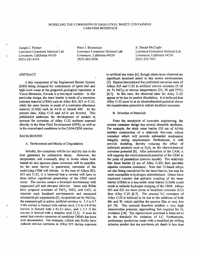
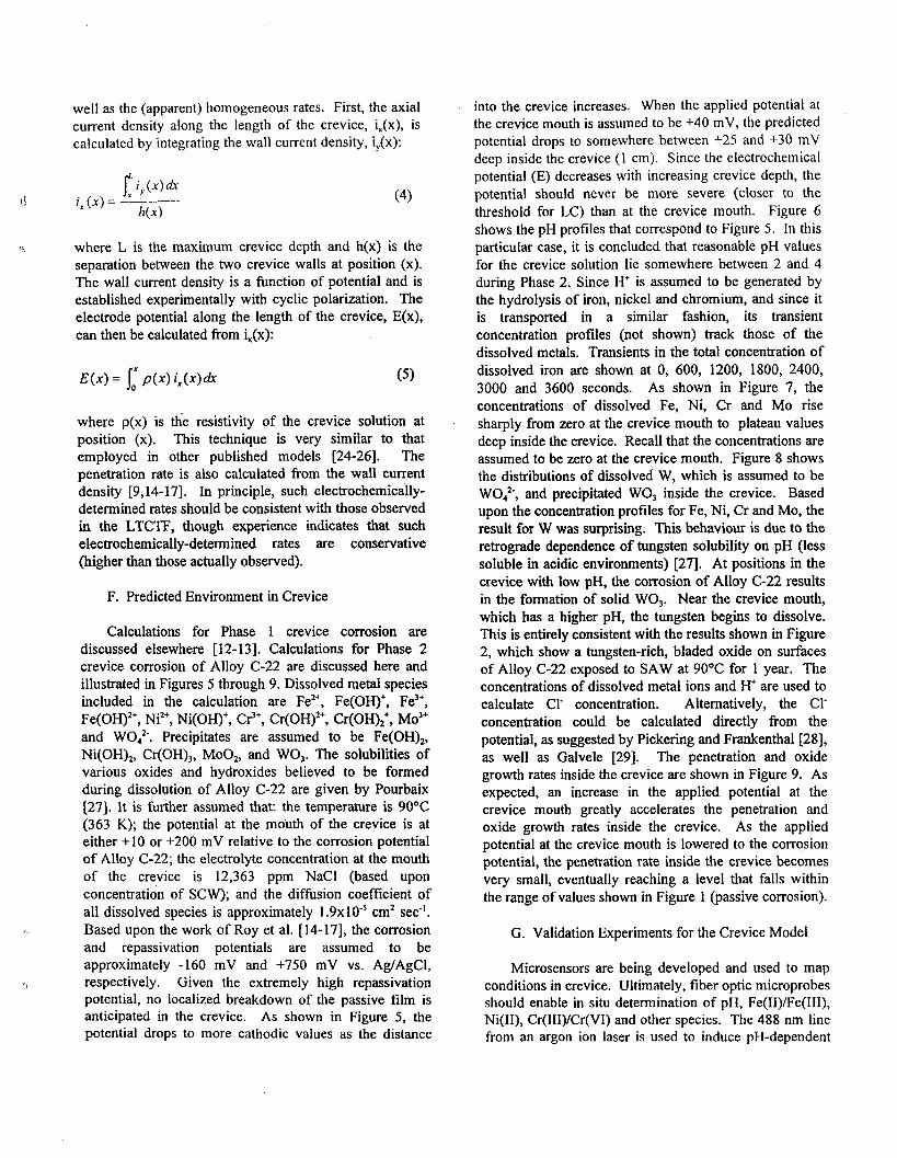
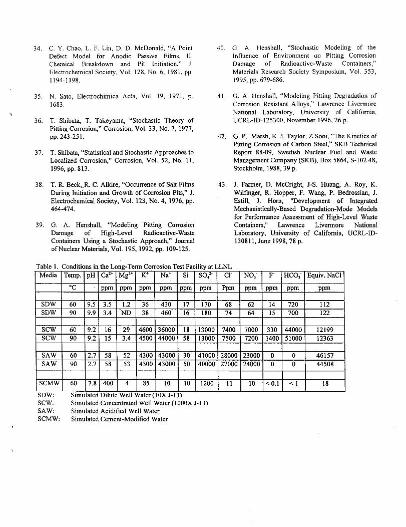
The modes of corrosion that are believed to be relevant to the ultimate failure of the CRM include: (a) passive corrosion; (b) crevice corrosion; (c) pitting; and (d) stress corrosion cracking. Passive corrosion of the CRM is expected to occur on surfaces where the CAM has exfoliated, as well as on surfaces that lie inside the CAM-CRM crevice, provided that environmental conditions (pH, chloride, potential, and temperature) are below the thresholds for localized attack. A correlation of Alloy C-22 passive corrosion rates with temperature, pH, equivalent NaCl concentration, and FeCI, concentration has been developed Ill]. The rates used as a basis of this correlation are from the LTCTF, Roy’s electrochemical measurements [ 14- 171, and Haynes International [6,7]. The following linear equation was found to be adequate for the correlation:

ln(z)=l3.409-(s)-0.87409($/) (1)

+ 0.56965@,)+ 0.608Ol(C,,,)

where Ap/At is the apparent penetration rate (pm yr-‘); T is the temperature (“C); CNaC, is the equivalent concentration of NaCl (wt. %); and C,,,, is the concentration of FeCl, (wt. %). Based upon this correlation, it is concluded that the apparent activation energy is approximately 12 kcal mot’, which is quite reasonable. The “standard error of estimate” (s~,,~,J and the “sample multiple variable regression coefficient” (ry~,234> are defined by Crow, Davis and Maxfield [IS]. The “standard error of estimate” is a measure of the scatter of the observed penetration rates about the regression plane. About 95% of the points in a large sample are expected to lie within tin,,,..,, of the plane, measured in the y direction. Values for the above correlation are:

s,,,,~,~ = 1.5092 rv,,234 = 0.65628

(2)

The “multiple variable regression coefficient” indicates a reasonably good fit to the dam set, given the large number of independent variables. This simple correlation has been tested within the bounds of anticipated conditions. As shown in Figure 1, the predictions appear to be reasonable for combinations of input parameters representative of the: Near Field Environment (NFE); Simulated Dilute Well (SDW), Simulated Concentrated Well (SCW), and Simulated Acidified Well (SAW) waters; Simulated Cement-Modified Water (SCMW); the unusually harsh, simulated crevice corrosion test of Haynes International (10 wt. % FeCl,) [6,7]; and the conditions predicted during preliminary tests of the LLNL crevice model.

B. Corrosion Products and Surface Morphology B. Crevice Corrosion Model

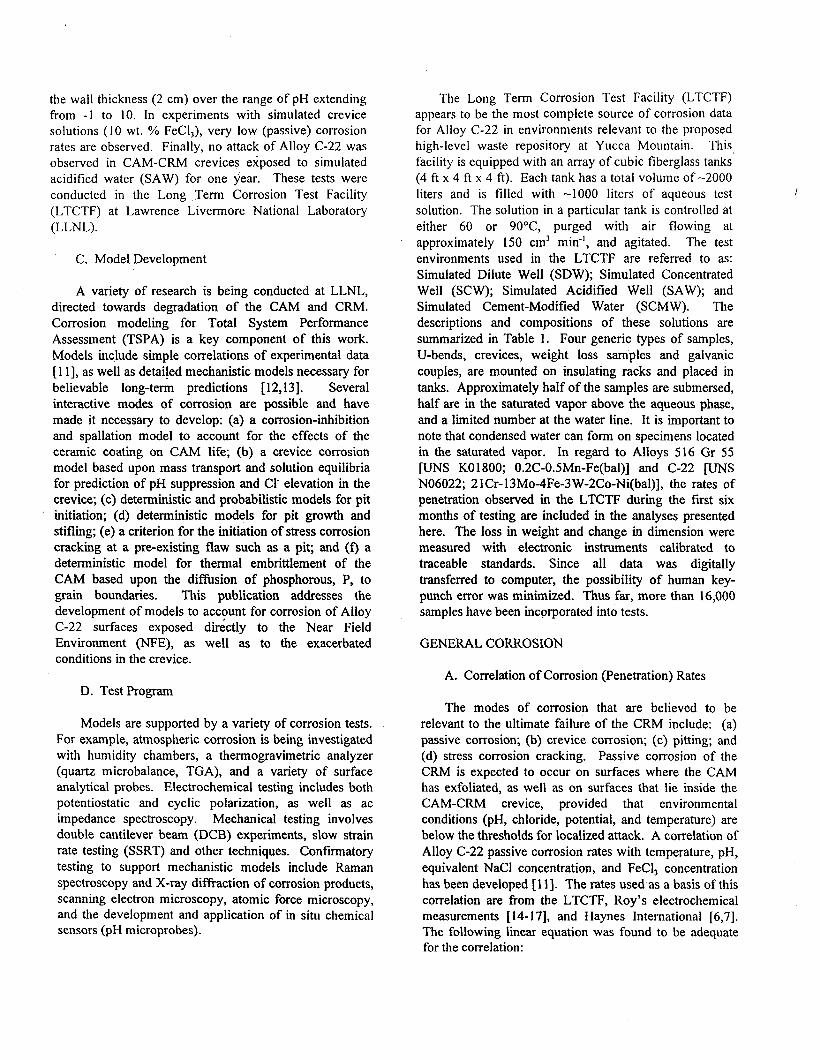
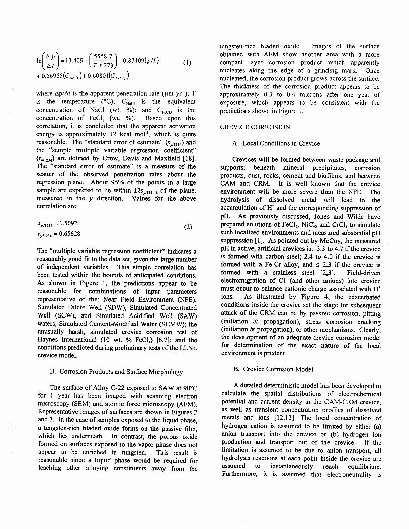
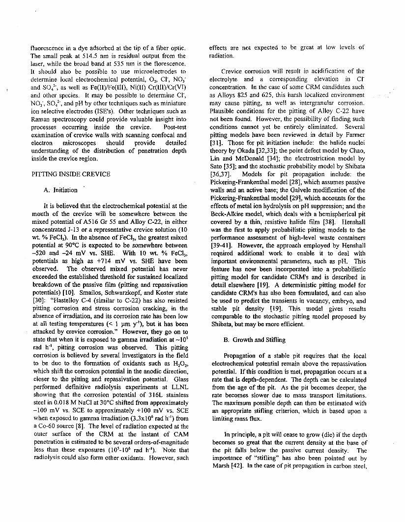
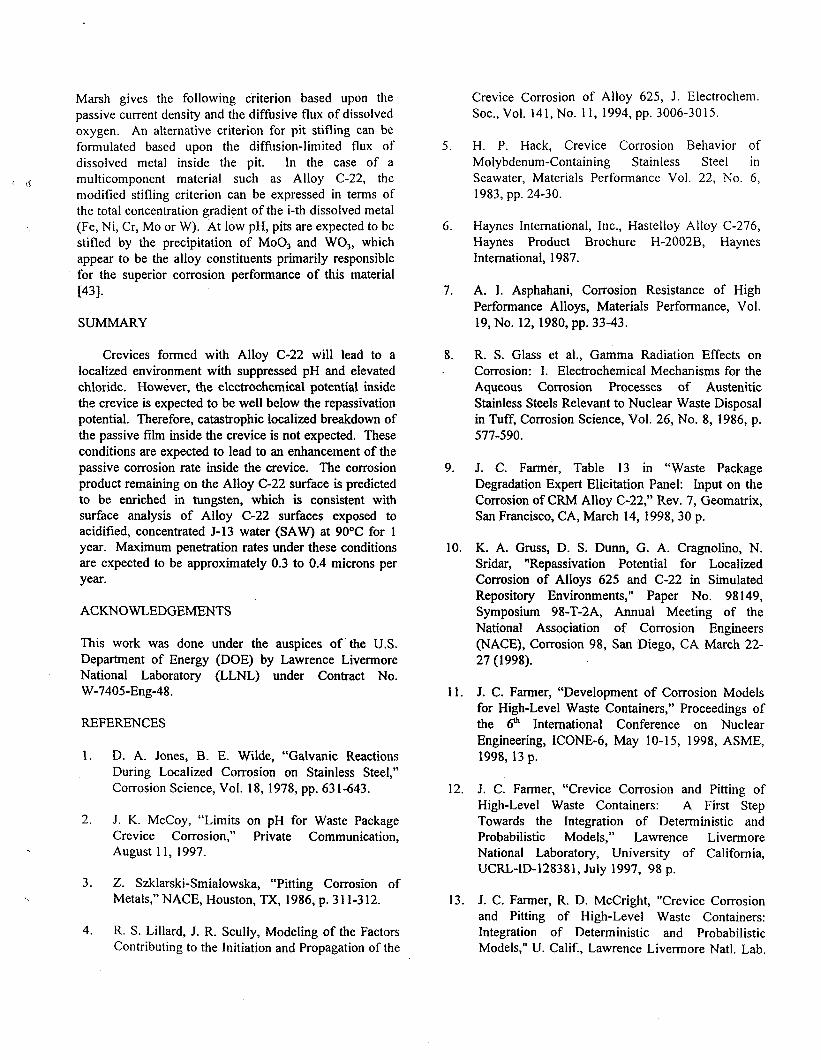
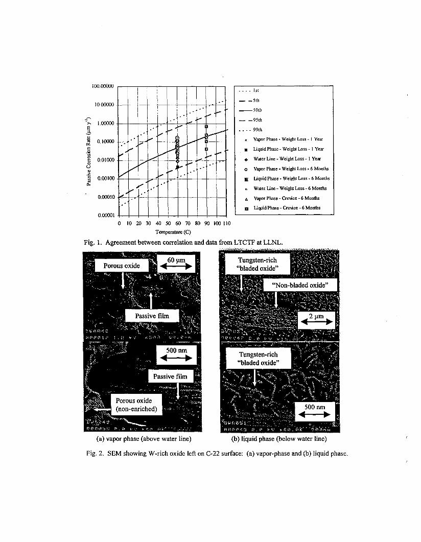
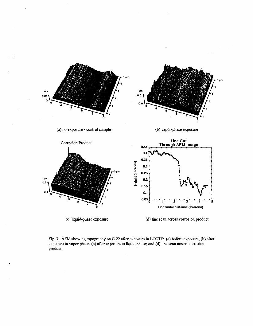
The surface of Alloy C-22 exposed to SAW at 90°C for 1 year has been imaged with scanning electron microscopy (SEM) and atomic force microscopy (AFM). Representative images of surfaces are shown in Figures 2 and 3. In the case of samples exposed to the liquid phase, a tungsten-rich bladed oxide forms on the passive film, which lies underneath. In contrast, the porous oxide formed on surfaces exposed to the vapor phase does not appear to be enriched in tungsten. This result is reasonable since a liquid phase would be required for leaching other alloying constituents away from the

tungsten-rich bladed oxide. Images of the surface obtained with AF&l show another area with a more compact layer corrosion product which apparently nucleates along the edge of a grinding mark. Once nucleated, the corrosion product grows across the surface. The thickness of the corrosion product appears to be approximately 0.3 to 0.4 microns after one year of exposure, which appears to be consistent with the predictions shown in Figure 1.

CREVICE CORROSION

A. Local Conditions in Crevice

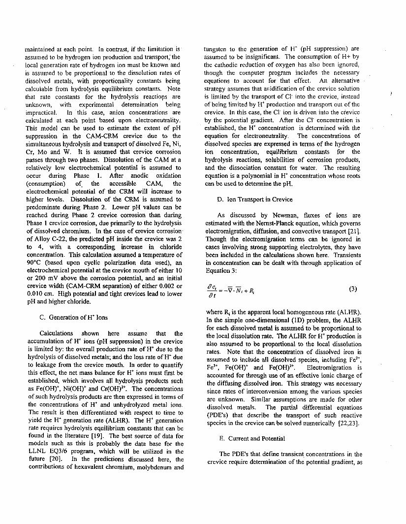
Crevices will be formed between waste package and supports; beneath mineral precipitates, corrosion products, dust, rocks, cement and biofilms; and between CAM and CRM. It is well known that the crevice environment will be more severe than the NFE. The hydrolysis of dissolved metal will lead to the accumulation of H’ and the corresponding suppression of pH. As previously discussed, Jones and Wilde have prepared solutions of FeCl,, NiCl, and CrCI, to simulate such localized environments and measured substantial pH suppression [l]. As pointed out by McCoy, the measured pH in active, artificial crevices is: 3.3 to 4.7 if the crevice is formed with carbon steel; 2.4 to 4.0 if the crevice is formed with a Fe-Cr alloy, and 5 2.3 if the crevice is formed with a stainless steel [2,3]. Field-driven electromigration of Cl- (and other anions) into crevice must occur to balance cationic charge associated with H’ ions. As illustrated by Figure 4, the exacerbated conditions inside the crevice set the stage for subsequent attack of the CRM can be by passive corrosion, pitting (initiation & propagation), stress corrosion cracking (initiation & propagation), or other mechanisms. Clearly, the development of an adequate crevice corrosion model for determination of the exact nature of the local environment is prudent.

A detailed deterministic model has been developed to calculate the spatial distributions of electrochemical potential and current density in the CAM-CRM crevice, as well as transient concentration profiles of dissolved metals and ions [ 12,131. The local concentration of hydrogen cation is assumed to be limited by either (a) anion transport into the crevice or (b) hydrogen ion production and transport out of the crevice. If the limitation is assumed to be due to anion transport, all hydrolysis reactions at each point inside the crevice are assumed to instantaneously reach equilibrium. Furthermore, it is assumed that electroneutrality is

maintained at each point. In contrast, if the limitation is assumed to be hydrogen ion production and transport,’ the local generation rate of hydrogen ion must be known and is assumed to be proportional to the dissolution rates of dissolved metals, with proportionality constants being calculable from hydrolysis equilibrium constants. Note that rate constants for the hydrolysis reactions are unknown, with experimental determination being impractical. In this case, anion concentrations are calculated at each point based upon electroneutrality. This model can be used to estimate the extent of pH suppression in the CAM-CRM crevice due to the simultaneous hydrolysis and transport of dissolved Fe, Ni, Cr, MO and W. It is assumed that crevice corrosion passes through two phases. Dissolution of the CAM at a relatively low electrochemical potential is assumed to occur during Phase 1. After anodic oxidation (consumption) of- the accessible CAM, the electrochemical potential of the CRM will increase to higher levels. Dissolution of the CRM is assumed to predominate during Phase 2. Lower pH values can be reached during Phase 2 crevice corrosion than during Phase 1 crevice corrosion, due primarily to the hydrolysis of dissolved chromium. In the case of crevice corrosion of Alloy C-22, the predicted pH inside the crevice was 2 to 4, with a corresponding increase in chloride concentration. This calculation assumed a temperature of 90°C (based upon cyclic polarization data used), an electrochemical potential at the crevice mouth of either 10 or 200 mV above the corrosion potential, and an initial crevice width (CAM-CRM separation) of either 0.002 or 0.010 cm. High potential and tight crevices lead to lower pH and higher chloride.

C. Generation of H’ Ions

Calculations shown here assume that the accumulation of H’ ions (pH suppression) in the crevice is limited by: the overall production rate of H’ due to the hydrolysis of dissolved metals; and the loss rate of H’ due to leakage from the crevice mouth. In order to quantify this effect, the net mass balance for H’ ions must first be established, which involves all hydrolysis products such as Fe(OH)‘, Ni(OH)’ and Cr(OH)‘+. The concentrations of such hydrolysis products are then expressed in terms of the concentrations of H’ and unhydrolyzed metal ions. The result is then differentiated with respect to time to yield the H’ generation rate (ALHR). The H’ generation rate requires hydrolysis equilibrium constants that can be found in the literature [19]. The best source of data for models such as this is probably the data base for the LLNL EQ3/6 program, which will be utilized in the future [20]. In the predictions discussed here, the contributions of hexavalent chromium, molybdenum and

tungsten to the generation of H’ (pH suppression) are assumed to be insignificant. The consumption of H+ by the cathodic reduction of oxygen has also been ignored, though the computer program includes the necessary equations to account for that effect. An alternative strategy assumes that acidification of the crevice solution is limited by the transport of Cl- into the crevice, instead of being limited by H’ production and transport out of the crevice. In this case, the Cl ion is driven into the crevice by the potential gradient, After the Cl concentration is established, the H’ concentration is determined with the equation for electroneutrality. The concentrations of dissolved species are expressed in terms of the hydrogen ion concentration, equilibrium constants for the hydrolysis reactions, solubilities of corrosion products, and the dissociation constant for water. The resulting equation is a polynomial in H’ concentration whose roots can be used to determine the pH.

D. Ion Transport in Crevice

As discussed by Newman, fluxes of ions are estimated with the Nemst-Planck equation, which governs electromigration, diffusion, and convective transport [2 11. Though the electromigration terms can be ignored in cases involving strong supporting electrolytes, they have been included in the calculations shown here. Transients in concentration can be dealt with through application of Equation 3 :

where R is the apparent local homogeneous rate (ALHR). In the simple one-dimensional (1 D) problem, the ALHR for each dissolved metal is assumed to be proportional to the local dissolution rate. The ALHR for H’ production is also assumed to be proportional to the local dissolution rates. Note that the concentration of dissolved iron is assumed to include all dissolved species, including Fe”, Fe’+, Fe(OH)’ and Fe(OH)“. Electromigration is accounted for through use of an effective ionic charge of the difI%sing dissolved iron. This strategy was necessary since rates of interconversion among the various species are unknown. Similar assumptions are made for other dissolved metals. The partial differential equations (PDE’s) that describe the transport of such reactive species in the crevice can be solved numerically [22,23].

E. Current and Potential

The PDE’s that define transient concentrations in the crevice require determination of the potential gradient, as

well as the (apparent) homogeneous rates. First, the axial current density along the length of the crevice, i,(x), is calculated by integrating the wall current density, i,(x):

i,(x) = I” I i,(x)&

h(x) (4)

where L is the maximum crevice depth and h(x) is the separation between the two crevice wails at position (x). The wall current density is a function of potential and is established experimentally with cyclic polarization. The electrode potential along the length of the crevice, E(x), can then be calculated from i,(x):

(5)

where p(x) is the resistivity of the crevice solution at position (x). This technique is very similar to that employed in other published models [24-261. The penetration rate is also calculated from the wall current density [9,14-171. In principle, such electrochemically- determined rates should be consistent with those observed in the LTCTF, though experience indicates that such electrochemically-determined rates are conservative (higher than those actually observed).

F. Predicted Environment in Crevice

Calculations for Phase 1 crevice corrosion are discussed elsewhere [ 12- 131. Calculations for Phase 2 crevice corrosion of Alloy C-22 are discussed here and illustrated in Figures 5 through 9. Dissolved metal species included in the calculation are Fe”, Fe(OH)“, Fe3’, Fe(OH)2’, Ni’+, Ni(OH)‘, Cr”, Cr(OH)2’, Cr(OH)2+, MO” and W0,2‘. Precipitates are assumed to be Fe(OH),, Ni(OH),, Cr(OH),, MOO,, and WO,. The solubilities of various oxides and hydroxides believed to be formed during dissolution of Alloy C-22 are given by Pourbaix [27]. It is further assumed that: the temperature is 90°C (363 K); the potential at the mouth of the crevice is at either +lO or +200 mV relative to the corrosion potential of Alloy C-22; the electrolyte concentration at the mouth of the crevice is 12,363 ppm NaCl (based upon concentration of SCW); and the diffusion coefftcient of all dissolved species is approximately 1.9x l@’ cm2 set“. Based upon the work of Roy et al. [ 14-171, the corrosion and repassivation potentials are assumed to be approximately -160 mV and +750 mV vs. Ag/AgCl, respectively. Given the extremely high repassivation potential, no localized breakdown of the passive film is anticipated in the crevice. As shown in Figure 5, the potential drops to more cathodic values as the distance

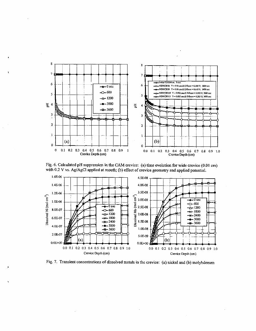
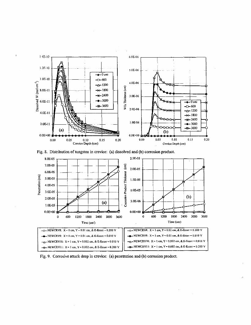
into the crevice increases. When the applied potential at the crevice mouth is assumed to be +40 mV, the predicted potential drops to somewhere between +25 and +30 mV deep inside the crevice (1 cm). Since the electrochemical potential (E) decreases with increasing crevice depth, the potential should never be more severe (closer to the threshold for LC) than at the crevice mouth. Figure 6 shows the pH profiles that correspond to Figure 5. In this particular case, it is concludedthat reasonable pH values for the crevice solution lie somewhere between 2 and 4 during Phase 2. Since H’ is assumed to be generated by the hydrolysis of iron, nickel and chromium, and since it is transported in a similar fashion, its transient concentration profiles (not shown) track those of the dissolved metals. Transients in the total concentration of dissolved iron are shown at 0, 600, 1200, 1800, 2400, 3000 and 3600 seconds. As shown in Figure 7, the concentrations of dissolved Fe, Ni, Cr and MO rise sharply from zero at the crevice mouth to plateau values deep inside the crevice. Recall that the concentrations are assumed to be zero at the crevice mouth. Figure 8 shows the distributions of dissolved W, which is assumed to be WO,‘-, and precipitated WO, inside the crevice. Based upon the concentration profiles for Fe, Ni, Cr and MO, the result for W was surprising. This behaviour is due to the retrograde dependence of tungsten solubility on pH (less soluble in acidic environments) 1271. At positions in the crevice with low pH, the corrosion of Alloy C-22 results in the formation of solid WO,. Near the crevice mouth, which has a higher pH, the tungsten begins to dissolve. This is entirely consistent with the results shown in Figure 2, which show a tungsten-rich, bladed oxide on surfaces of Alloy C-22 exposed to SAW at 90°C for 1 year. The concentrations of dissolved metal ions and H’ are used to calculate Cl concentration. Alternatively, the Cl concentration could be calculated directly from the potential, as suggested by Pickering and Frankenthal [28], as well as Galvele [29]. The penetration and oxide growth rates inside the crevice are shown in Figure 9. As expected, an increase in the applied potential at the crevice mouth greatly accelerates the penetration and oxide growth rates inside the crevice. As the applied potential at the crevice mouth is lowered to the corrosion potential, the penetration rate inside the crevice becomes very small, eventually reaching a level that falls within the range of values shown in Figure 1 (passive corrosion).

G. Validation Experiments for the Crevice Model

Microsensors are being developed and used to map conditions in crevice. Ultimately, fiber optic microprobes should enable in situ determination of pH, Fe(II)/Fe(III), Ni(II), Cr(III)/Cr(VI) and other species. The 488 nm line from an argon ion laser is used to induce pH-dependent

fluorescence in a dye adsorbed at the tip of a fiber optic. The small peak at 514.5 nm is residual output from the laser, while the broad band at 535 nm is the florescence. It should also be possible to use microelectrodes to determine local electrochemical potential, O,, Cl‘, NO,‘ and SOb2-, as well as Fe(II)/Fe(III), Ni(I1) Cr(IlI)/Cr(VI) and other species. It may be possible to determine Cl, NO,‘, S0,2-, and pH by other techniques such as miniature ion selective electrodes (ISE’s). Other techniques such as Raman spectroscopy could provide valuable insight into processes occurring inside the crevice. Post-test examination of crevice walls with scanning confocal and electron microscopes should provide detailed understanding of the distribution of penetration depth inside the crevice region.

PITTING INSIDE CREVICE

A. Initiation -

It is believed that the electrochemical potential at the mouth of the crevice will be somewhere between the mixed potential of A516 Gr 55 and Alloy C-22, in either concentrated J- 13 or a representative crevice solution (10 wt. % FeCl,). In the absence of FeCl,, the greatest mixed potential at 90°C is expected to be somewhere between -520 and -24 mV vs. SHE. With 10 wt. % FeCl,, potentials as high as +714 mV vs. SHE have been observed. The observed mixed potential has never exceeded the established threshold for sustained localized breakdown of the passive film (pitting and repassivation potentials) [lo]. Smailos, Schwarzkopf, and Koster state [30]: “Hastelloy C-4 (similar to C-22) has also resisted pitting corrosion and stress corrosion cracking, in the absence of irradiation, and its corrosion rate has been low at all testing temperatures (C 1 pm ye’), but it has been attacked by crevice corrosion.” However, they go on to state that when it is exposed to gamma irradiation at -10’ rad h-‘, pitting corrosion was observed. This pitting corrosion is believed by several investigators in the field to be due to the formation of oxidants such as H202, which shift the corrosion potential in the anodic direction, closer to the pitting and repassivation potential. Glass performed definitive radiolysis experiments at LLNL showing that the corrosion potential of 3 16L stainless steel in 0.0 18 M NaCl at 30°C shifted from approximately -100 mV vs. SCE to approximately +I00 mV vs. SCE when exposed to gamma irradiation (3.3~10~ rad h’) from a Co-60 source [8]. The level of radiation expected at the outer surface of the CRM at the instant of CAM penetration is estimated to be several orders-of-magnitude less than these exposures (lo’- 1 O6 rad h“). Note that radiolysis could also form other oxidants. However, such

effects are not expected to be great at low levels of radiation.

Crevice corrosion will result in acidification of the electrolyte and a corresponding elevation in Cl concentration. In the case of some CRM candidates such as Alloys 825 and 625, this harsh localized environment may cause pitting, as well as intergranular corrosion. Plausible conditions for the pitting of Alloy C-22 have not been found. However, the possibility of finding such conditions cannot yet be entirely eliminated. Several pitting models have been reviewed in detail by Farmer [31]. Those for pit initiation include: the halide nuclei theory by Okada [32,33]; the point defect model by Chao, Lin and McDonald [34]; the electrostriction model by Sato [35]; and the stochastic probability model by Shibata [36,37]. Models for pit propagation include: the Pickering-Frankenthal model [28], which assumes passive walls and an active base; the Galvele modification of the Pickering-Frankenthal model [29], which accounts for the effects of metal ion hydrolysis on pH suppression; and the Beck-Alkire model, which deals with a hemispherical pit covered by a thin, resistive halide film [38]. Henshall was the first to apply probabilistic pitting models to the performance assessment of high-level waste containers [39-41]. However, the approach employed by Henshall required additional work to enable it to deal with important environmental parameters, such as pH. This feature has now been incorporated into a probabilistic pitting model for candidate CRM’s and is described in detail elsewhere [ 193. A deterministic pitting model for candidate CRM’s has also been formulated, and can also be used to predict the transients in vacancy, embryo, and stable pit density [ 191. This model gives results comparable to the stochastic pitting model proposed by Shibata, but may be more efficient.

B. Growth and Stifling

Propagation of a stable pit requires that the local electrochemical potential remain above the repassivation potential. If this condition is met, propagation occurs at a rate that is depth-dependent. The depth can be calculated from the age of the pit. As the pit becomes deeper, the rate becomes slower due to mass transport limitations. The maximum possible depth can then be estimated with an appropriate stifling criterion, which is based upon a limiting mass flux.

In principle, a pit will cease to grow (die) if the depth becomes so great that the current density at the base of the pit falls below the passive current density. The importance of “stifling” has also been pointed out by Marsh [42]. In the case of pit propagation in carbon steel,

’ \t

‘I

Marsh gives the following criterion based upon the passive current density and the diffusive flux of dissolved oxygen. An alternative criterion for pit stifling can be formulated based upon the diffusion-limited flux of dissolved metal inside the pit. In the case of a multicomponent material such as Alloy C-22, the modified stifling criterion can be expressed in terms of the total concentration gradient of the i-th dissolved metal (Fe, Ni, Cr, MO or W). At low pH, pits are expected to be stifled by the precipitation of MOO, and WO,, which appear to be the alloy constituents primarily responsible for the superior corrosion performance of this material [431.

SUMMARY

Crevices formed with Alloy C-22 will lead to a localized environment with suppressed pH and elevated chloride. However, the electrochemical potential inside the crevice is expected to be well below the repassivation potential. Therefore, catastrophic localized breakdown of the passive film inside the crevice is not expected. These conditions are expected to lead to an enhancement of the passive corrosion rate inside the crevice. The corrosion product remaining on the Alloy C-22 surface is predicted to be enriched in tungsten, which is consistent with surface analysis of Alloy C-22 surfaces exposed to acidified, concentrated J-13 water (SAW) at 90°C for 1 year. Maximum penetration rates under these conditions are expected to be approximately 0.3 to 0.4 microns per year.

ACKNOWLEDGEMENTS

This work was done under the auspices of the U.S. Department of Energy (DOE) by Lawrence Livermore National Laboratory (LLNL) under Contract No. W-7405-Eng-48.

REFERENCES

1. D. A. Jones, B. E. Wilde, “Galvanic Reactions During Localized Corrosion on Stainless Steel,” Corrosion Science, Vol. 18, 1978, pp. 631-643.

2. J. K. McCoy, “Limits on pH for Waste Package Crevice Corrosion,” Private Communication, August 11, 1997.

3. Z. Szklarski-Smialowska, “Pitting Corrosion of Metals,” NACE, Houston, TX, 1986, p. 3 1 l-3 12.

4. R. S. Lillard, J. R. Scully, Modeling of the Factors Contributing to the Initiation and Propagation of the

5.

6.

7.

8.

9.

10.

11.

12.

13.

Crevice Corrosion of Alloy 625, J. Electrochem. Soc.,Vol. 141,No. 11, 1994,~~. 3006-3015.

H. P. Hack, Crevice Corrosion Behavior of Molybdenum-Containing Stainless Steel in Seawater, Materials Performance Vol. 22, No. 6, 1983, pp. 24-30.

Haynes International, Inc., Hastelloy Alloy C-276, Haynes Product Brochure H-2002B, Haynes International, 1987.

A. I. Asphahani, Corrosion Resistance of High Performance Alloys, Materials Performance, Vol. 19, No. 12, 1980, pp. 33-43.

R. S. Glass et al., Gamma Radiation Effects on Corrosion: I. Electrochemical Mechanisms for the Aqueous Corrosion Processes of Austenitic Stainless Steels Relevant to Nuclear Waste Disposal in Tuff, Corrosion Science, Vol. 26, No. 8, 1986, p. 577-590.

J. C. Farmer, Table 13 in “Waste Package Degradation Expert Elicitation Panel: Input on the Corrosion of CRM Alloy C-22,” Rev. 7, Geomatrix, San Francisco, CA, March 14, 1998,30 p.

K. A. Gruss, D. S. Dunn, G. A. Cragnolino, N. Sridar, “Repassivation Potential for Localized Corrosion of Alloys 625 and C-22 in Simulated Repository Environments,” Paper No. 98149, Symposium 98-T-2A, Annual Meeting of the National Association of Corrosion Engineers (NACE), Corrosion 98, San Diego, CA March 22- 27 (1998).

J. C. Farmer, “Development of Corrosion Models for High-Level Waste Containers,” Proceedings of the 6* International Conference on Nuclear Engineering, ICONE-6, May 10-15, 1998, ASME, 1998, 13 p.

J. C. Farmer, “Crevice Corrosion and Pitting of High-Level Waste Containers: A First Step Towards the Integration of Deterministic and Probabilistic Models,” Lawrence Livermore National Laboratory, University of California, UCRL-ID-128381, July 1997, 98 p.

J. C. Farmer, R. D. McCright, “Crevice Corrosion and Pitting of High-Level Waste Containers: Integration of Deterministic and Probabilistic Models,” U. Calif., Lawrence Livermore Natl. Lab.

14.

15.

16.

17.

18.

19.

20.

21.

22.

23.

24.

Rept. No. UCRL-ID-127980, Part 1, 24 p, October 13, 1997; Paper No. 98 160, Symposium 9%T-2A, Annual Meeting of the National Association of Corrosion Engineers (NACE), Corrosion 98, San Diego, CA March 22-27 (1998).

A. K. Roy, D. L. Fleming, B. Y. Lum, “Effect of Environmental Variables on Localized Corrosion of High-Performance Container Materials,” Lawrence Livermore National Laboratory, University of California, UCRL-JC- 125329, January 1997, 16 p.

A. K. Roy, D. L. Fleming, B. Y. Lum, “Localized Corrosion of Container Materials in Anticipated Repository Environments,,’ Lawrence Livermore National Laboratory, University of California, UCRL-JC-122861, May 1996, 10 p.

A. K. Roy,- D. L. Fleming, B. Y. Lum, “Electrochemical and Metallographic Evaluation of Alloy C-22 and 625,“’ Lawrence Livermore National Laboratory, University of California, UCRL-ID- 127355, May 1997, 10 p.

A. K. Roy, D. L. Fleming, B. Y. Lum, Unpublished Data, 1997.

E. L. Crow, F. A. Davis, M. W. Maxfield, Statistics Manual, Dover Publications, Inc., New York, NY, 1960, pp. 147-19.

J. W. Oldfield, W. H. Sutton, “Crevice Corrosion of Stainless Steels: I. A Mathematical Model,” British Corrosion Journal, Vol. 13, No. 1, 1978, pp. 13-22.

J. C. Walton, G. Cragnoliino, S. K. Kalandros, “A Numerical Model of Crevice Corrosion for Passive and Active Metals,” Corrosion Science, Vol. 38, No. 1, 1996, pp. l-18.

J. S. Newman, Electrochemical Svstems, 2nd Ed., Prentice Hall, Englewood Cliffs, NJ, 199 1.

V. G. Jenson, G. V. Jeffreys, Mathematical Methods in Chemical Engineering, Academic Press, New York, NY, 1963, pp. 410-422.

D. D. McCracken, W. S. Dom, Numerical Methods and Fortran Programming with Applications in Science and Engineering, John Wiley and Sons, New York, NY, 1964, pp. 377-385.

P. 0. Gartland, “A Simple Model of Crevice Corrosion Propagation for Stainless Steels in Sea

25.

26.

27.

28.

29.

30.

31.

32.

33.

Water,” Corrosion 97, Paper No. 417, National Association of Corrosion Engineers, Houston, TX, 1997, 17 p.

Y. Xu, H. W. Pickering, “The Initial Potential and Current Distributions of the Crevice Corrosion! Process,” J. Electrochemical Society, Vol. 140, No. 3, 1993, pp. 658-668.

E. A. Nystrom, J. B. Lee, A. A. Sagues, H. W. Pickering, “An Approach for Estimating Anodic Current Distributions in Crevice Corrosion from Potential Measurements,” J. Electrochemical Society, Vol. 141,No. 2, 1994, pp. 358-361.

M. Pourbaix, Atlas of Electrochemical Equilibria in Aqueous Solutions, English Translation by J. A. Franklin, Pergamon Press, New York, NY; Cebelcor, Brussels, Belgium, 1966,644 p.

H. W. Pickering, R. P. Frankenthal, “On the Mechanism of Localized Corrosion of Iron and Stainless Steel: I. Electrochemical Studies,,’ J. Electrochemical Society, Vol. 119, No. 10, 1972, pp. 1297-1304.

J. R. Galvele, “Transport Processes and the Mechanism of Pitting of Metals,” J. Electrochemical Society, Vol. 123, No. 4, 1976, pp. 464-474.

E. Smailos, W. Schwarzkopf, R. Koster, “Corrosion Behaviour of Container Materials for the Disposal of High-Level Wastes in Rock Salt Formations,” Nuclear Science and Technology, Commission of the European Communities, DUR 10400, 1986.

J. C. Farmer, G. E. Gdowski, R. D. McCright, H. S. Ahluwahlia, “Corrosion Models for Performance Assessment of High-Level Radioactive-Waste Containers,” Nuclear Engineering Design, Vol. 129, 199 1, pp. 57-88.

T. Okada, “Halide Nuclei Theory of Pit Initiation in Passive Metals, J. Electrochemical Society, Vol. 131, No. 2, 1984, pp. 241-247.

T. Okada, “A Theory of Perturbation-Initiated Pitting, Proceedings of the International Symposium Honoring Professor Marcel Pourbaix on his Eightieth Birthday: Equilibrium Diagrams and Localized Corrosion, R. P. Frankenthal, J. Kruger, Eds., Electrochemical Society, Pennington, NJ, Vol. 84-9, 1984, pp. 402-43 1.

34. C. Y. Chao, L. F. Lin, D. D. McDonald, “A Point Defect Model for Anodic Passive Films, II. Chemical Breakdown and Pit Initiation,” J. Electrochemical Society, Vol. 128, NO. 6, 1981, pp. 1194-l 198.

'1

35. N. Sato, Electrochimica Acta, Vol. 19, 1971, p. 1683.

36. T. Shibata, T. Takeyama, “Stochastic Theory of Pitting Corrosion,” Corrosion, Vol. 33, No. 7, 1977, pp. 243-25 1.

37. T. Shibata, “Statistical and Stochastic Approaches to Localized Corrosion,” Corrosion, Vol. 52, No. 11, 1996, pp. 813.

38. T. R. Beck,-R. C. Alkire, “Occutrence of Salt Films During Initiation and Growth of Corrosion Pits,,, J. Electrochemical Society, Vol. 123, No. 4, 1976, pp. 464-474.

39. G. A. Henshall, “Modeling Pitting Corrosion Damage of High-Level Radioactive-Waste Containers Using a Stochastic Approach,,, Journal of Nuclear Materials, Vol. 195, 1992, pp. 109-125.

40.

41.

42.

43.

G. A. Henshall, “Stochastic Modeling of the Influence of Environment on Pitting Corrosion Damage of Radioactive-Waste Containers,” Materials Research Society Symposium, Vol. 353, 1995, pp. 679-686.

G. A. Henshall, “Modeling Pitting Degradation of Corrosion Resistant Alloys,” Lawrence Livermore National Laboratory, University of California, UCRL-ID-125300, November 1996’26 p.

G. P. Marsh, K. J. Taylor, Z Sooi, “The Kinetics of Pitting Corrosion of Carbon Steel,” SKB Technical Report 88-09, Swedish Nuclear Fuel and Waste Management Company (SKB), Box 5864, S- 102 48, Stockholm, 1988’39 p.

J. Farmer, D. McCright, J-S. Huang, A. Roy, K. Wilfinger, R. Hopper, F. Wang, P. Bedrossian, J. Estill, J. Horn, “Development of Integrated Mechanistically-Based Degradation-Mode Models for Performance Assessment of High-Level Waste Containers,” Lawrence Livermore National Laboratory, University of California, UCRL-ID- 130811, June 1998’78 p.

Table 1. Conditions in the Long-Term Corrosion Test Facility at LLNL

SDW: Simulated Dilute Well Water (1 OX J- 13) sew: Simulated Concentrated Well Water (1000X J- 13) SAW: Simulated Acidified Well Water SCMW: Simulated Cement-Modified Water

,

loo.ccooO

lO.COOOO

% 1.00000 E

s

3 O.lcooO

.B

fi 0.01ooo 8 .$

2 O.oolGQ

o.oco1o

O.ooool

- _ _ _ 1st

- -5th

-50th

- -95th

_ _ - . 99th

x Vapor Phase - Weight Loss - I Year

m Liquid Phase - Weight Loss - I Year

* Water Line - Weight Loss - 1 Year

0 Vapor Phase - Wci&t Lass - 6 Months

6 Liquid Phase - Weight Loss - 6 Months

D Water Line - Weight Loss - 6 Months

6. Vapor Phase - Credce - 6 Months

q Liquid Phase - Credce - 6 Months

0 10 20 30 40 50 60 70 80 90 100110

Temperature (C)

Fig. 1. Agreement between correlation and data from LTCTF at LLNL.

Passive film I

4 Porous oxide (non-enriched)

Tungsten-rich “bladed oxide”

(a) vapor phase (above water line) (b) liquid phase (below water line)

Fig. 2. SEM showing W-rich oxide left on C-22 surface: (a) vapor-phase and (b) liquid phase.

nm

180

0 1

0

(a) no exposure - control sample

Corrosion Product

(c) liquid-phase exposure

5 (rm

m

0.3

\ 0.0

(b) vapor-phase exposure

Line Cut Through AFM Image o.a5,....,....,....,....,....,

0.4 .

0.35 f !? 0.3

g 025 r----l

;I ,,,,,,,,,,. y , 1 2 3 4 5

Horizontal distance (microns)

(d) line scan across corrosion product

Fig. 3. AFM showing topography on C-22 after exposure in LTCTF: (a) before exposure; (b) after exposure in vapor phase; (c) after exposure to liquid phase; and (d) line scan across corrosion product.

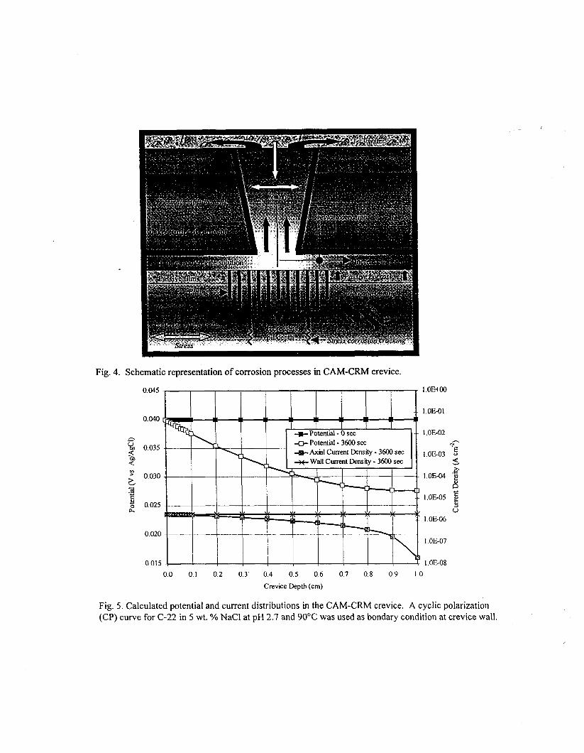
Fig. 4. Schematic representation of corrosion processes in CAM-CRM crevice.

0.045 -

0.040

2 0.035 + Potential - 3600 xc 5 + *Wall Axial Current Current Density Density - - 3600 3600 set set

2 5

0.030

3 2 2 0.025 ---t--~-+-+----,--.+---l a

0.020

1 .OE+oo

I .OE02

7 I.OE03 g

5

I.0504 P

1

1.OE05 ii 5

v

I OE08

0.0 0.1 0.2 0.3 0.4 0.5 0.6 0.7 0.8 0.9 I.0

Crevice Depth (cm)

Fig. 5. Calculated potential and current distributions in the CAM-CRM crevice. A cyclic polarization (CP) curve for C-22 in 5 wt. % NaCl at pH 2.7 and 90°C was used as bondary condition at crevice wall.

6

5

z4

3

2

1

0

x CL

-O-~~~.Y=0.0lun&LEsorr=O.KY)V; 36oOrsc +NEWCRW Y=0.01cm&LEmr=0.010V. 3K0ssc ~Nl3'/Cl&'IO Y=0.OMan&E~~=0.010V:3600sce n

1 i @I i i i i i i i I I 0 0.1 0.2 0.3 0.4 0.5 0.6 0.7 0.8 0.9 1 0.0 0.1 0.2 0.3 0.4 0.5 0.6 0.7 0.8 0.9 1.0

Crevice Depth (cm) Crevice Depth (cm)

Fig. 6. Calculated pH suppression in the CAM crevice: (a) time evolution for wide crevice (0.01 cm) with 0.2 V vs. Ag/AgCl applied at mouth; (b) effect of crevice geometry and applied potential.

1.6EO6 4.5E-08

1.4EO6 4.OM8

‘E ; 1.0~06 5 '5 8.OE07

5 6.OEO7 .B a 4.OE07

2.OE-07

O.OE+OO

'$ 3.OE-08 z .%2.X-08

l--L- I -Lose0 I I x/ J&l -0-m *1200

8 B 2.OE-08 1. i? 1.5Ft-08 8

i.OE-08

5.oEm

O.OE+CG 0.0 0.1 0.2 0.3 0.4 0.5 0.6 0.7 0.8 0.9 1.0 0.0 0.1 0.2 0.3 0.4 0.5 0.6 0.7 0.8 0.9 1.0

Crevice Depth (cm) Crevice Depth (cm)

Fig. 7. Transient concentrations of dissolved metals in the crevice: (a) nickel and (b) molybdenum

1.4E-IO 6.OL06

1.2E-IO S.OE-06

l.OE-10 T

$ z .5 8.0511

3 3 6.OE-11

4 .a

n 4.oE-II

4.OE-06

-2 s I

3 3.OE-06 .o

F?,

2 2.OE-06

I .OE-06

O.OE+OC 1 O.OE+C!O 0.00 0.05 0.10 0.15 0.20 0.00 0.05 0.10 0.15 0.20

Crevice Depth (cm) Crc\icc Depth (cm)

Fig. 8. Distribution of tungsten in crevice: (a) dissolved and (b) corrosion product.

0 600 1200 1800 2400 3ooO 3600 0 600 1200 1800 2400 3ooO 3600

2.5LQ5

-2 * 2.OE-05

1

2‘2 1.5E-05 e

4 -8 1.OE-05 k

O.OE+OO

Time (set) Time (see)

+NEWCRVt?: X = I cm, Y = 0.01 cm. & E-Ecorr = 0.200 V eNEWCRV8: X = 1 cm. Y = 0.01 cm. & E-Eeorr = 0.200 V

+NEWCRW: X = I cm. Y = 0.01 cm, & E-F.corr = 0.010 V +NEWCRW: X= I cm.Y=O.Ol cm.&E-Ecorr=O.OIOV

+NEWCRVIO: X=Icm,Y=O.O02cm,&E-F.eorr=O.OlOV +N!ZWCRVIO: X=icm,Y=O.O02cm,&E-Ec.orr=O.OlOV

+NEWCRVl I : X = I cm, Y = 0.002 cm, & E-Ecorr = 0.200 V

Fig. 9. Corrosive attack deep in crevice: (a) penetration and (b) corrosion product.