Modeling the formation of bright slope deposits associated

Modeling the formation of bright slope deposits associated with gulliesin Hale Crater, Mars: Implications for recent liquid water

Kelly Jean Kolb a,*, Jon D. Pelletier a,b, Alfred S. McEwen a

aDepartment of Planetary Sciences/Lunar and Planetary Laboratory, University of Arizona, 1629 E. University Blvd., Tucson, AZ 85721, USAbDepartment of Geosciences, University of Arizona, 1040 E. 4th St., Tucson, AZ 85721, USA

a r t i c l e i n f o

Article history:Received 31 October 2008Revised 29 August 2009Accepted 1 September 2009Available online 29 September 2009

Keywords:Mars, SurfaceGeological processesMars

a b s t r a c t

Our study investigates possible formation mechanisms of the very recent bright gully deposits (BGDs)observed on Mars in order to assess if liquid water was required. We use two models in our assessment:a one-dimensional (1D) kinematic model to model dry granular flows and a two-dimensional (2D) fluid-dynamic model, FLO-2D (O’Brien et al., 1993, FLO Engineering), to model water-rich and wet sediment-rich flows. Our modeling utilizes a high-resolution topographic model generated from a pair of imagesacquired by the High Resolution Imaging Science Experiment (HiRISE) aboard the Mars ReconnaissanceOrbiter. For the 1D kinematic modeling of dry granular flows, we examine a range of particle sizes, flowthicknesses, initial velocities, flow densities, and upslope initiation points to examine how these param-eters affect the flow run-out distances of the center of mass of a flow. Our 1D modeling results show thatmultiple combinations of realistic parameters could produce dry granular flows that travel to within theobserved deposits’ boundaries. We run the 2D fluid-dynamic model, FLO-2D, to model both water-richand wet sediment-rich flows. We vary the inflow volume, inflow location, discharge rate, water-loss rate(water-rich models only), and simulation time and examine the resulting maximum flow depths andvelocities. Our 2D modeling results suggest that both wet sediment-rich and water-rich flows could pro-duce the observed bright deposits. Our modeling shows that the BGDs are not definitive evidence ofrecent liquid water on the surface of Mars.

� 2009 Elsevier Inc. All rights reserved.

1. Introduction

Although Mars appears dry and barren today, there is abundantevidence that it was wetter in its past. The discovery of the martiangullies (Malin and Edgett, 2000) by the Mars Orbiter Camera (MOC,Malin and Edgett, 2001) aboard the Mars Global Surveyor (MGS,Albee et al., 1998) raised the possibility that liquid water was pres-ent on the martian surface in geologically recent times, within thepast 1 Ma (Malin and Edgett, 2000). It was initially proposed thatthe gullies formed by groundwater seepage from a subsurfaceaquifer because of their similarities to terrestrial seepage gullies(Malin and Edgett, 2000). Since this original proposal, gully forma-tion has been frequently debated, with no single theory capable ofexplaining all of the observed characteristics. The High ResolutionImaging Science Experiment (HiRISE) (McEwen et al., 2007b) cam-era aboard the Mars Reconnaissance Orbiter (MRO) has revealedunprecedented details of gullies down to a pixel scale of 25 cm/pix-el, providing new clues about gully formation (McEwen et al.,2007a; Gulick and the HiRISE Team, 2008).

1.1. Gully characteristics

Malin and Edgett (2000) defined a martian gully to be a small-scale feature (generally less than a few km long) with an alcove,channel, and debris apron. Often martian gullies are much largerthan terrestrial gullies and are evolved landforms with multiplechannels on their floors, such that they might be better termed ra-vines or gulches (Wilson, 1900, pp. 36–39). Material is thought tohave been removed from the alcove, transported through the chan-nel, and deposited in a fan at the base of the slope. Gullies arefound on mid-latitude slopes, including mesas, troughs, and craterwalls. They are also found in polar pits, on crater central peaks, onisolated mounds, and on dunes. Gullies, by the Malin and Edgett(2000) definition, are occasionally found in equatorial regions aswell. Gullies have a wide range of morphologies, ranging from nar-row, shallow channels to wide, deeply incised and developed chan-nel systems. Their source regions can be short and wide, long andnarrow, or barely resolvable (Malin and Edgett, 2000). Many gullieshave characteristics reminiscent of terrestrial fluvial features,including terraces, point bars, braided channels, and sinuous chan-nels (Gulick and McEwen, 2007). Gullies often contain overlappingand crosscutting channels and debris aprons, which implies that

0019-1035/$ - see front matter � 2009 Elsevier Inc. All rights reserved.doi:10.1016/j.icarus.2009.09.009

* Corresponding author. Address: 1629 E. University Blvd., Room 325, Box 244,Tucson, AZ 85721, USA. Fax: +1 520 621 4933.

E-mail address: [email protected] (K.J. Kolb).

Icarus 205 (2010) 113–137

Contents lists available at ScienceDirect

Icarus

journal homepage: www.elsevier .com/locate / icarus

multiple flow episodes in a given channel system are common. Al-coves are thought to expand through undermining and collapse.Boulders are often concentrated in gully channels, which is sugges-tive of a flow that preferentially transports smaller particles (McE-wen et al., 2007a).

Many gullies are relatively young; they are extremely sparselycratered and their debris aprons are often superposed on otheryoung features such as dunes and polygonal ground (Malin andEdgett, 2000). The gullies are not all pristine; many gullies haveexperienced aeolian, mass wasting, and periglacial modificationsince their formation. The relative youth of the gullies makes themparticularly intriguing. How these features with potential fluvialcharacteristics formed recently in a low pressure, low temperatureenvironment that rarely (Hecht, 2002) permits the existence of li-quid water remains a mystery.

1.2. An overview of gully erosional agents

Gully formation theories center around different erosionalagents. Several theories invoke liquid water, but the origin of thiswater varies. Malin and Edgett (2000) proposed that the wateroriginates from a shallow subsurface aquifer and seeps onto thesurface. Hartmann et al. (2003) suggested that the aquifer’s wateris released due to local geothermal heating events. Gaidos (2001)put forth the idea that water in a deep pressurized aquifer couldbe transported to the surface through the aqueous equivalents ofdikes and sills. Lee et al. (2001) and Christensen (2003) proposedthat melting snow pack could generate run-off to form gullies. Cos-tard et al. (2002) suggested that melting near-surface ground icecould form the gullies. Gilmore and Phillips (2002) suggested thataquicludes could transport melting ice to slope faces. Mellon andPhillips (2001) and Knauth and Burt (2002) theorized that brinesmight form the gullies because of the ability of salts to depressthe freezing point of a liquid.

Carbon dioxide and dry granular material have also been in-voked as gully erosional agents. Musselwhite et al. (2001) andHoffman (2002) suggested that a carbon dioxide suspended flowcould erode the gullies, but Stewart and Nimmo (2002) and Urqu-hart and Gulick (2003) found that a sufficient carbon dioxide reser-voir should not exist on present-day Mars and Stewart and Nimmo(2002) also noted that the expected morphology of CO2 gulliesdoes not match what is observed. Formation of gullies by ava-lanches of granular CO2 ice was described by Ishii et al. (2006).Treiman (2003) proposed that dry aeolian material deposited onthe lee side of slopes moves downslope and carves gullies, and Bart(2007) suggested that dry landslides could produce certain gullies.

Each proposed erosional agent and related formation hypothe-ses involving the proposed agents has certain strengths and weak-nesses (see Treiman, 2003; Heldmann and Mellon, 2004;Heldmann et al., 2007 for reviews). It is not required that all gulliesform by the same mechanism, and it has been suggested (Held-mann et al., 2008b) that different classes of gullies have unique for-mation mechanisms. However, it is probable that the majority ofgullies within each class form in the same way given their overallsimilarities in morphology. For this study, we focus on a particularclass of gullies, those with recent relatively bright deposits.

1.3. Bright gully deposits

Malin et al. (2006) reported the discovery of newly formed, rel-atively bright, deposits in two martian gullies and proposed thatthe new deposits were evidence that liquid water reaches or formson the surface of Mars today in sufficient quantities to cause a flow.These two new bright gully deposits (BGDs) formed near pre-exist-ing channels (Malin et al., 2006) and thus represent gully activity(McEwen et al., 2007a) but not necessarily gully formation. Gully

‘‘activity” refers to a flow that occurs within a gully, while gully‘‘formation” refers to a flow that creates or carves a gully. Sincethe BGDs were not observed to carve new channels, they werenot necessarily emplaced by the same mechanism that drives gullyformation. The new deposits both occur in well-preserved craterswith steep walls and depth-to-diameter ratios typical of their ori-ginal form (McEwen et al., 2007a; Kolb et al., 2007). The underlyinggullies are very narrow, shallow, and pristine. The gullies with thenew BGDs are among the most pristine in their setting, whichmight suggest that their host walls are the most recent sites ofgully activity. There are some bright deposits associated with gul-lies that have noticeable modification in the form of bright aeolianripples (Fig. 1); these are not currently thought to be related to therecent, unmodified BGDs.

Several interpretations have been offered for why the depositsare bright. Malin et al. (2006) proposed that the deposits might con-tain ice, frost, fine-grained materials, or precipitates and that thebrightness of an ice or frost deposit could be maintained if ice isreplenished from within the deposit or another source. Williamset al. (2007) evaluated the scenario of a water-rich deposit existingat the observed new BGD locations. Theymodeled the lifetime of anice-rich deposit at the locations of the new BGDs and found that athin ice-rich deposit would completely sublimate in less than twomartian years, a shorter time than the deposits have been observedto exist. HiRISE re-imaged the BGDs multiple times and did not de-tect any significant changes in shape or contrast as would be ex-pected if they were composed of water ice. The CompactReconnaissance Imaging Spectrometer for Mars (CRISM, Murchie

Fig. 1. A relatively old bright deposit associated with a gully. Left shows the entiregully and bright deposit. Right shows a closer view of the deposit. Aeolian andpossible periglacial (Mellon, 1997) modification can be seen. HiRISE imagePSP_001846_2390, equirectangular projection centered at 57.8�N, 82.4�E,0.312 m/pixel, in Utopia Planitia. North in this, and all following images, is upunless otherwise indicated.

114 K.J. Kolb et al. / Icarus 205 (2010) 113–137

et al., 2007), the visible to infrared spectrometer aboard MRO, hasnot detected any ice or hydrated minerals in the deposits (McEwenet al., 2007a; Barnouin-Jha et al., 2008). Hydratedmineralsmight beexpected if liquid water transported the material; however, theirexistence would not be diagnostic of a water-rich flow because awet or dry flow could have transported pre-existing hydrated orunhydrated minerals from steep upper slopes. Heldmann et al.(2008a) proposed that the deposits are remnant mudflows thattransported fine grains. Given the lack of evidence for ice or evapor-ites, it is most likely that the deposits are bright because they con-tain fine-grained materials or because inherently bright materialswere transported by the flow (McEwen et al., 2007a; Pelletieret al., 2008). It is important to note that the new deposits are lo-cated in relatively dark regions compared to Mars globally, whichhas an average albedo of �0.20. Williams et al. (2007) estimatedthe albedos of the deposits to be 0.15 and 0.20 and the surroundingterrains to be 0.13 and 0.189 for the Naruko Crater and PentictonCrater deposits, respectively. The bright gully deposits would ap-pear dark if they formed in a relatively bright region of Mars.

1.4. Previous related work

Previous studies (Lanza and Gilmore, 2006; Dickson et al., 2007;Parsons et al., 2008) examined the average slopes on which gulliesare located and incorrectly stated that, if the average slope is belowthe angle of repose (�26.4–32.78�, determined experimentally byPouliquen, 1999), then a completely dry formation mechanism isruled out. This assumption neglects the fact that the upslope re-gions of concave slopes are steeper than the average slope andpotentially steeper than the angle of repose. Heldmann and Mellon(2004) looked at the average slopes of the walls adjacent to gullyalcoves using interpolated Mars Orbiter Laser Altimeter (MOLA,aboard MGS, Zuber et al., 1992) topography data and found theaverage slopes to be typically less than the angle of repose. Theyclaimed that the calculated slopes rule out mass wasting as thedominant mechanism that forms gully alcoves but noted thatpost-gully modification within steepened alcoves could occur bymass wasting. Average source region slopes are not necessarilyrepresentative of actual source regions due to the extended natureof the alcoves, which can extend up to �1.5 km (Heldmann andMellon, 2004). The average slopes in the above-mentioned workswere derived using MOLA topography that has an along-trackspacing of �300 m and a footprint size of �168 m (Neumannet al., 2001). Given that gully channels are observed down to thelimit of resolution (less than 1 m), there is a large scale differencebetween MOLA footprints and the features of interest. High-resolu-tion topography is needed to best model and understand gulliesand their formation mechanisms.

Pelletier et al. (2008) used high-resolution topography to modelpossible formation mechanisms of the Penticton Crater BGD. Theyused a 1 m/post digital elevation model (DEM) of the PentictonCrater BGD from a HiRISE stereo pair created using the methodsof Kirk et al. (2008) and used one-dimensional kinematic modelingand two-dimensional fluid-dynamic modeling to assess the forma-tion of the Penticton Crater BGD. Their modeling indicated that acompletely dry flow could explain the location and morphologyof the deposit. Given the difficulty of producing liquid water onthe martian surface today (Mellon and Phillips, 2001), Pelletieret al. (2008) concluded that the Penticton Crater deposit was likelyemplaced by a dry granular flow. Pelletier et al. (2008) pointed outthe important distinction between the angle of static friction(�26.4–32.76�, determined experimentally by Pouliquen, 1999),commonly called the angle of repose (Nicholson, 1838, p. 36;McClung and Schaerer, 2006, p. 87), and the angle of kinetic friction(20.7–22.9�, determined experimentally by Pouliquen, 1999), be-low which all dry, non-fluidized flows will decelerate. The distinc-

tion is that a flow on a slope with an angle between the kinetic andstatic friction angles will not spontaneously start but will continueto flow if already moving with sufficient momentum. This showsthat, as long as an upslope region is steeper than the angle of re-pose for the slope’s material, then a dry granular flow could flowon a shallower slope without depositing until the slope is approx-imately the angle of kinetic friction.

1.5. Current study

Our study extends the work of Pelletier et al. (2008) to twoBGDs located in Hale Crater (Fig. 2). Hale Crater has a large numberof gullies and multiple BGDs (Fig. 3), hereafter identified basedupon their designation in Fig. 3. No high-resolution images wereacquired with HiRISE or MOC before the bright deposits in Haleformed, but the deposits have no resolvable modification andtherefore are presumably young. While most of the Hale gulliescontain characteristics that may be interpreted as fluvial, thisstudy focuses only on the formation of the BGDs. An analysis ofslopes hosting BGDs (Kolb et al., 2007) found that the Hale BGDshad the lowest average slopes and therefore were the best candi-dates for deposits requiring liquid water. However, higher resolu-tion topography was needed to determine if the source regionwas below the angle of repose. We use a high-resolution topo-graphic model created from a stereo pair of HiRISE images toexamine the slopes where the BGDs formed and to model their for-mation using one-dimensional kinematic modeling of dry granularflows and two-dimensional fluid-dynamic modeling of water-richand wet sediment-rich flows. We model wet flows to see if wecan rule out the presence of water during the formation of BGDs.The overarching goal of this project is to test the hypothesis thatsignificant quantities of liquid water reached the surface of Marsin today’s climate by modeling the formation of the BGDs.

The remainder of this document is organized as follows:Section 2 describes the types of data used. Section 3 details how weselected our study region. Section 4 contains observations of theHale BGDs. Section 5 includes methods and results from an analy-sis of HiRISE color images of the BGDs. Section 6 includes modeldetails, modeling methods, and results for our 1D kinematic mod-eling of dry granular flows. Section 7 includes model details, mod-eling methods, and results for our 2D fluid-dynamic modeling of

Fig. 2. Hale Crater, Mars. The rectangle shows the approximate area of the BGDs(Fig. 3) and the DEM (Fig. 4). The BGDs are concentrated near and in the DEM’sboundaries. Hale Crater is 125 km � 150 km and centered near 35.8�S, 323.5�E.THEMIS Day IR mosaic, 256 pixels per degree.

K.J. Kolb et al. / Icarus 205 (2010) 113–137 115

water-rich and wet sediment-rich flows. Section 8 contains a dis-cussion of our results and possible implications. Section 9 summa-rizes our work and conclusions.

2. Data

2.1. Imagery

This study used MOC, HiRISE, and Context Camera (CTX, aboardMRO, Malin et al., 2007) images acquired at visible wavelengths.MOC images have pixel scales of �1.5–6 m/pixel, while CTX imagesare typically 5–6 m/pixel. HiRISE images have a smaller field ofview than CTX images at a pixel scale as fine as 25 cm/pixel. Thebulk of the analysis in this study comes from HiRISE imagesPSP_002932_1445 and PSP_003209_1445 (Table 1). The HiRISEimages were processed using the Integrated Software for Imagersand Spectrometers (ISIS3) developed by the United States Geolog-ical Survey in Flagstaff, Arizona (Anderson et al., 2004). The CTXimages were used to survey Hale Crater for gullies and BGDs be-cause full crater coverage was available. MOC and CTX images

were used in conjunction with HiRISE images for multitemporalanalyses of the BGDs to look for changes in shape and tone.

2.2. Topography

The two types of elevation data used in this study are MOLAPrecision Experiment Data Records (PEDRs, Smith et al., 1998)and a high-resolution topographic model developed from theHiRISE stereo pair described in Table 1.

Fig. 3. Bright deposits associated with gullies in Hale Crater. The boxes mark the locations of the lettered insets. (A) BGD1. Left and right mark the upslope branches. (B)BGD2. (C) BGD3. Middle and right mark two of the upslope branches. (D) BGD4. The possible source alcoves of the bright flow are noted. See text for reasoning. HiRISE imagePSP_002932_1445, equirectangular projection centered at 35.16�S, 324.68�E, 0.255 m/pixel.

Table 1HiRISE images used to produce the digital elevation model.

Parameter PSP_002932_1445 PSP_003209_1445

Center latitude 35.16�S 35.13�SCenter longitude 324.68�E 324.69�ELs 199.19� 212.19�Emission angle 4.65� 20.390�Incidence angle 58.49� 56.65�Pixel scale (RED CCDs) 0.255 m/pixel 0.271 m/pixel


We obtained MOLA PEDRs from the Planetary Data System(PDS, McMahon, 1996) and extracted using PEDR2TAB (Softwareby G. Neumann) applying the crossover correction developed byNeumann et al. (2001). With the crossover correction applied,MOLA points have vertical errors less than 1 m and horizontalplacement errors of�100 m (Neumann et al., 2001). Between-trackspacing varies depending on latitude, being greater at the equator,and the orbit of the spacecraft.

The DEM used in this study (Fig. 4) was produced by Oded Aha-ronson’s group at Caltech using SOCET-SET’s (http://www.soc-etgxp.com/) area-based automatic image matching package andpreprocessing methods developed by Kirk et al. (2008). The DEMis 1 m/post and has an overall estimated vertical precision of�0.19 m although it contains larger matching errors in certainlocations without manual editing. Manual corrections of the DEMwere necessary to minimize errors produced by the automatedprocessing.

3. Site selection

HiRISE has observed several BGDs in addition to the ones dis-cussed in Malin et al. (2006) (McEwen et al., 2007a; Kolb et al.,2007). Table 2 lists characteristics of the BGDs studied by McEwenet al. (2007a) and Kolb et al. (2007). In most of these cases, thereare no high-resolution images that show these gullies before theformation of the bright deposits, but the deposits appear geomor-phologically identical to the two known examples that formed inthe past decade and have no resolvable modification down to HiR-ISE scales (�25 cm/pixel). There has not yet been a systematic glo-bal search for BGDs, so there is a possible selection bias in ouranalysis. BGDs were distinguished from typical gully debris apronsbased on distinct albedo differences from their surroundings. TheBGDs occur near the end of a gully channel and sometimes alongthe sides of channels, indicating that the flow level was higher thanthe local channel depth or that dust lofted by the flow extended be-yond the channel. Identification of BGDs is limited by image cover-age, quality, and resolution. The BGDs of interest are presently onlythose without any resolvable modification, leading to the assump-tion that they formed recently. Overall, the BGDs are located onsteep average slopes, close to the angle of repose, with the actualdeposits lying on shallower portions downslope.

The BGDs are typically located in well-preserved craters. Inevery case, there are obvious bright layers upslope that are a likelysource of the transported material. The bright deposits observed inPenticton Crater and Hale Crater are extremely thin, below the res-olution of HiRISE DEMs with vertical precisions of �16 cm and

�19 cm for the Penticton Crater and Hale DEMs, respectively (Kirket al., 2008). The deposits are elongated and consist of digitatelobes (Malin et al., 2006). HiRISE images show that the flows some-times overtopped obstacles (Fig. 5) and sometimes were deflectedby them. Overall, the distribution of the deposits appears moreconsistent with a dry granular flow (e.g., a dust avalanche) than awet density current. In the following sections, we use numericalmodels to test this qualitative suggestion.

Hale Crater was chosen based on an analysis of average slopesof gullies containing BGDs on Mars summarized in Table 2. Theaverage slopes were determined by overlaying MOLA points ontop of HiRISE images with a method developed by Kolb and Okubo(in press) or using shadow lengths measured in the down-Sundirection, where available. The BGDs in Hale Crater are likelyamong the best candidates for liquid water given their relativelylow average slopes, which is why we selected them for our studyand produced a DEM at this location.

4. Observations

4.1. Hale Crater

Hale Crater (Fig. 2) is a large 125 � 150 km impact crater lo-cated in the southern hemisphere of Mars. Hale Crater is inter-preted as Late Hesperian/Early Amazonian (Cabrol et al., 2001)but might be younger (Tornabene et al., 2008). It is possibly themost pristine crater of its size based on crater counts and morpho-logical features interpreted as primary, including ponded and pit-ted material (Tornabene et al., 2008). Hale Crater contains a largenumber of gullies on multiple slope orientations, which is fairlyrare on Mars. There are also gullies on its central peak and on bothsides of part of its rim (Dickson and Head, 2005; Dickson et al.,2007). None of the gullies in Hale Crater imaged by HiRISE havesuperposed craters, indicating that the gullies formed well afterthe impact event, perhaps even within the last million years assuggested by Malin and Edgett (2000) for gullies globally.

4.2. Hale Crater BGDs

Hale Crater has four bright slope deposits associated with gul-lies, BGDs, on its northeast rim (Figs. 2 and 3). Unlike other gullieswith BGDs around Mars, the Hale Crater BGDs are not narrow andshallow and have abundant evidence of multiple flows (Kolb et al.,2007). BGD1, BGD2, and BGD3 lie on top of debris aprons, butBGD4 stops midslope. The BGDs start midslope even though thegully channels extend most of the slope’s length. The BGDs followthe underlying channels and in some locations appear to haveovertopped the channels, depositing bright material along thechannel banks (Fig. 8).

Near the BGDs, the upper rim of Hale consists of eroding out-crops that are breaking into boulders (Fig. 6). A large concentrationof boulders is seen in Fig. 6 to clog the middle branch of BGD3’s al-cove. Several of the BGD channels have a high concentration ofboulders relative to surrounding terrain. Most of the bouldersfound in the gullies are probably the result of post-gully formationmass wasting. Some of the boulders in the left branch of BGD1(Figs. 3A and 7) have bright material on them suggesting that theywere present during movement of the bright flow but preferen-tially left behind as the flow transported finer particles.

The underlying channel systems are rather complex and welldeveloped. Several of the channels contain features interpretedas fluvial, including bars, braided channels, streamlined islands,and terraces (McEwen et al., 2007a; Gulick et al., 2007). Fine chan-nels are also visible in several of the other gullies on Hale Crater’snortheast rim (HiRISE image PSP_002932_1445), west rim (HiRISE

Fig. 4. Hale Crater digital elevation model: perspective view. HiRISE imagePSP_002932_1445 (Fig. 3) overlaid on the DEM. The vertical exaggeration is fivetimes, and the vertical scale ranges from �1170 to 1130 m. The DEM is 1 m/post.Since BGD4 is located at the edge of PSP_002932_1445 (Fig. 3), it is cut off and notincluded in the DEM.


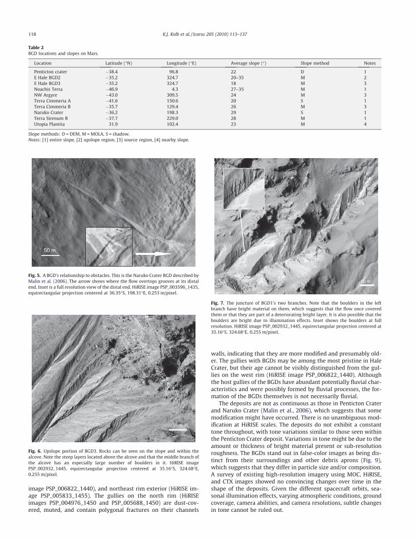
image PSP_006822_1440), and northeast rim exterior (HiRISE im-age PSP_005833_1455). The gullies on the north rim (HiRISEimages PSP_004976_1450 and PSP_005688_1450) are dust-cov-ered, muted, and contain polygonal fractures on their channels

walls, indicating that they are more modified and presumably old-er. The gullies with BGDs may be among the most pristine in HaleCrater, but their age cannot be visibly distinguished from the gul-lies on the west rim (HiRISE image PSP_006822_1440). Althoughthe host gullies of the BGDs have abundant potentially fluvial char-acteristics and were possibly formed by fluvial processes, the for-mation of the BGDs themselves is not necessarily fluvial.

The deposits are not as continuous as those in Penticton Craterand Naruko Crater (Malin et al., 2006), which suggests that somemodification might have occurred. There is no unambiguous mod-ification at HiRISE scales. The deposits do not exhibit a constanttone throughout, with tone variations similar to those seen withinthe Penticton Crater deposit. Variations in tone might be due to theamount or thickness of bright material present or sub-resolutionroughness. The BGDs stand out in false-color images as being dis-tinct from their surroundings and other debris aprons (Fig. 9),which suggests that they differ in particle size and/or composition.A survey of existing high-resolution imagery using MOC, HiRISE,and CTX images showed no convincing changes over time in theshape of the deposits. Given the different spacecraft orbits, sea-sonal illumination effects, varying atmospheric conditions, groundcoverage, camera abilities, and camera resolutions, subtle changesin tone cannot be ruled out.

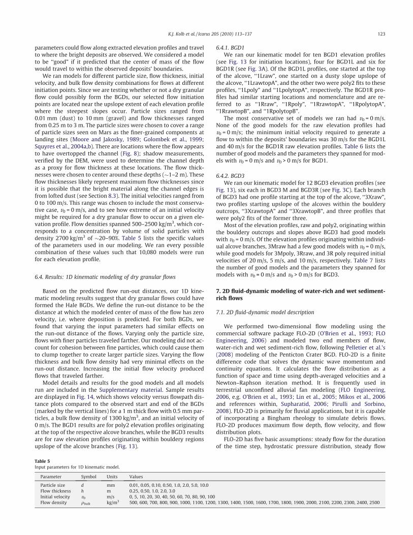
Table 2BGD locations and slopes on Mars.

Location Latitude (�N) Longitude (�E) Average slope (�) Slope method Notes

Penticton crater �38.4 96.8 22 D 1E Hale BGD2 �35.2 324.7 20–35 M 2E Hale BGD3 �35.2 324.7 18 M 3Noachis Terra �46.9 4.3 27–35 M 1NW Argyre �43.0 309.5 24 M 3Terra Cimmeria A �41.6 150.6 20 S 1Terra Cimmeria B �35.7 129.4 26 M 3Naruko Crater �36.2 198.3 29 S 1Terra Sirenum B �37.7 229.0 28 M 1Utopia Planitia 31.9 102.4 23 M 4

Slope methods: D = DEM, M = MOLA, S = shadow.Notes: [1] entire slope, [2] upslope region, [3] source region, [4] nearby slope.

Fig. 5. A BGD’s relationship to obstacles. This is the Naruko Crater BGD described byMalin et al. (2006). The arrow shows where the flow overtops grooves at its distalend. Inset is a full resolution view of the distal end. HiRISE image PSP_003596_1435,equirectangular projection centered at 36.35�S, 198.31�E, 0.253 m/pixel.

Fig. 6. Upslope portion of BGD3. Rocks can be seen on the slope and within thealcove. Note the steep layers located above the alcove and that the middle branch ofthe alcove has an especially large number of boulders in it. HiRISE imagePSP_002932_1445, equirectangular projection centered at 35.16�S, 324.68�E,0.255 m/pixel.

Fig. 7. The juncture of BGD1’s two branches. Note that the boulders in the leftbranch have bright material on them, which suggests that the flow once coveredthem or that they are part of a deteriorating bright layer. It is also possible that theboulders are bright due to illumination effects. Inset shows the boulders at fullresolution. HiRISE image PSP_002932_1445, equirectangular projection centered at35.16�S, 324.68�E, 0.255 m/pixel.


4.3. Individual deposits

BGD1 (Fig. 3A) has two main channel branches in its alcove,hereafter known as BGD1L (left branch) and BGD1R (right branch).Both branches have resolvable channels on their bottoms andbright material along the channel walls (Fig. 7). There is an outcropcontaining bright layers to the north side of the left branch. Theright branch does not have any bright layers upslope, but there isan abundance of bright material near the upslope end of the chan-nel. The fine channel in the left alcove branch is easily traced to thebranch juncture but beyond that it is difficult to determine whichof the many channels on the gully floor is the most recent. Themost continuous part of the bright deposit starts near a potentialbar, although bright material was deposited on top of streamlinedfeatures on the channel floor upslope of here. The flow appears tohave deposited bright material on the channel walls and marginsin downslope locations where it overtopped the channel(Fig. 8A). If the flow was largely dry, this overbank deposit mightbe from a dilute gravity current (i.e., a cloud of dust) moving withbut above the main flow.

The channel of BGD2 (Fig. 3B) can be traced upslope to anoutcrop that does not have bright layers. Bright material isabundant where the gully becomes more incised and a finechannel is first seen. Mid-channel regions have multiple terracesand a streamlined island. There is no distinct fine channel on thechannel floor; it is possible that it is below resolution limits(<�0.75 m) or has been infilled by aeolian deposits. The channelwalls are dusted with bright material in a discontinuous manner.The actual deposit starts near a series of terraces located nearthe base of the slope (Fig. 10). BGD2 is the least distinct of thosestudied.

BGD3 (Fig. 3C) has three branches in its alcove. Only the mid-dle and right branches, hereafter BGD3M (middle) and BGD3R(right), have traceable channels. There is an eroding outcrop con-taining bright layers upslope of the alcove (Fig. 6). The middlebranch has bright material lining its south wall and a remnantrockfall, rockslide or avalanche clogging it near the outcrop. Thechannels in the two branches cannot be distinguished from eachother in terms of age. The main channel contains streamlined is-lands, terraces, and multiple channels. The bright deposit starts

Fig. 8. Shadow measurements where flow overtopped banks. (A) BGD1 (Fig. 3A). (B) BGD3 (Fig. 3C). Shadows were measured, where available, where the flow appears tohave overtopped the channel and deposited along the banks. The numbers and arrows indicate where shadows were measured. HiRISE image PSP_002932_1445,equirectangular projection centered at 35.16�S, 324.68�E, 0.255 m/pixel.

Fig. 9. Bright gully deposits in color. The BGDs stand out compared to their surroundings, which suggests a difference in materials and/or particle sizes. (A) BGD1 (Fig. 3A). (B)BGD4 (Fig. 3D). HiRISE image PSP_003209_1445, equirectangular projection centered at 35.13�S, 324.69�E, 0.542 m/pixel.


approximately midslope and has a diffuse end. It appears to over-top a terrace at its start (Fig. 11).

BGD4 (Fig. 3D) is located at the south edge of the sceneimaged by HiRISE. Its alcove contains numerous channels. Thedeposit traces back up to the left side of the alcove where finechannels are seen as well as bright material (Fig. 3D). BGD4 isthe only BGD studied that stops midslope and does not followthe pre-existing channel’s path. The fact that BGD4 does notfollow the pre-existing channel is indicative of a flow with ahigher velocity and/or lower density than the flows that carvedthe underlying channel, which supports our belief that the BGDsdid not form the same way that gullies did. There are terracesand multiple channels on the gully floor. The deposit startswhere the two main groups of channels in the alcove meetdownslope. BGD4 is the most continuous of the BGDs observedin this study.

5. Color image analysis

5.1. Color measurements

Using the HiRISE images described in Table 1, we performed aquantitative color analysis to seek evidence that the compositionof the BGDs was markedly different from other surrounding mate-rial and bright material upslope. HiRISE has near-infrared (IR), red(R), and blue–green (BG) bands. The color swath of HiRISE imagescovers approximately 1.2 km at the center of the scene imaged. Theradiometric calibration of processed HiRISE data is generally goodto ±20% absolute and approximately 2% relative within an observa-tion; within a single channel, the pixel-to-pixel radiance values arecorrect to about 0.5% (Delamare et al., 2009).

We imported HiRISE PDS products into ISIS3. We used ISIS3’sqview to view and extract data from the false-color images. Qviewdisplays pixel information and I/F values for each of the bandssimultaneously. We measured the bright deposits, dusty surround-ing areas, bright layers upslope, bright material upslope, and brightmaterial along the channel walls, as available. We made four mea-surements within each feature, and then averaged the four valuesfor each band. We ratioed the bands to each other to minimize illu-mination effects.

5.2. Quantitative color analysis results

The locations of the color measurements are listed in Table 3and shown in Fig. 12. The color analysis of HiRISE imagePSP_003209_1445 does not reveal any visibly significant differ-ences between dusty areas, the bright deposits, bright layers, andbright material upslope (Fig. 12). There is not much variability be-tween the ratios of the various bright materials. The composition ofbright materials upslope of BGDs appears comparable to the com-position of the downslope BGDs. In Fig. 12, the points for a givenband ratio move down the image from left to right. It appears thatthere might be a slight general decrease in scene color variation inthe BG band moving down the image.

In order to test the reliability of the color analysis at distinguish-ing differences using the ratio method, we repeated our methodsdescribed in Section 5.1 for HiRISE image PSP_004052_2045 inMawrth Vallis, a Noachian outflow channel shown to have largecompositional variations (Wray et al., 2008). Wray et al. (2008)reported that there are six layers of distinct composition in thenorthern wall of the four kilometer crater featured in this image.Wemeasured color I/F valueswithin each of these spectroscopicallydistinct layers, as indicated by the colored arrows in Wray et al.(2008, see their Fig. 3), and found that a larger variation in colorratios is present (Fig. 12) when compared to the BGD ratios. Thisconfirms our findings that there is little difference between the

Fig. 11. The upslope edge of BGD3. Fig. 3C shows all of BGD3. Note that the flowoverlaps the terrace. HiRISE image PSP_002932_1445, equirectangular projectioncentered at 35.16�S, 324.68�E, 0.255 m/pixel.

Table 3Regions measured in color.

ID Description

B1 Diffuse end of BGD1B2 Bright material on BGD2’s wallB3 Diffuse end of BGD3B4 Near the end of BGD3B5 Start of BGD3B6 Middle branch in BGD3’s alcoveB7 Layers above BGD3B8 Bright material on gully wall near BGD4B9 BGD4B10 Alcove above BGD4 (left branch)D1 General wall dustyD2 Dusty region near BGD1D3 Dusty debris apron underlying BGD1D4 Dusty region near BGD4

Fig. 10. Terraces associated with BGD2. Fig. 3B shows all of BGD2. The brightdeposit starts near where the multiple terraces are observed. HiRISE imagePSP_002932_1445, equirectangular projection centered at 35.16�S, 324.68�E,0.255 m/pixel.


compositions of bright material in the bright gully deposits andbright material elsewhere in the scene.

6. 1D kinematic modeling of dry granular flows

6.1. Elevation profile extraction

We extracted channel elevation profiles from the DEM usingRiverTools (http://www.rivertools.com/, RIVIX, LLC), a GIS applica-tion that has the capability to extract flow grids from high-resolu-tion topography. Prior to elevation extraction, we pre-processedthe DEM using a 3 � 3 low pass filter twice to minimize high fre-quency noise. The DEM has errors near BGD2 and cuts off BGD4,so only BGD1 and BGD3 profiles were extracted for modeling. ForBGD1 and BGD3, we generated flow grids then extracted elevationprofiles using the channel profile tool. We extracted elevation pro-files for two branches of each BGD, left (BGD1L) and right (BGD1R)for BGD1 (Fig. 3A) and middle (BGD3M) and right (BGD3R) forBGD3 (Fig. 3C). We also extracted elevation profiles starting ups-lope of the gully alcoves on dusty slopes and in bouldery outcrops,as available, to examine the possibility of flows initiating in theselocations. Fig. 13 shows the upslope initiation point of all extractedelevation profiles.

When RiverTools produces a flow grid, it applies hydrologicalcorrections so that a flow will always move downslope, which

can create artificial steps in elevation profiles. The artifacts arelikely enhanced for an imperfect DEM and over regions whererough small-scale topography occurs. The BGD3 profiles did nothave many visible steps, but the BGD1 profiles had a large numberof visible steps. In a DEM with small-scale errors, slope determina-tion at the smallest scale is very problematic. Artificial steps have amajor impact on the modeling because they can cause the flow tostop near the initiation points (i.e. before the flow has acquired suf-ficient momentum to flow through small, artificial steps in theDEM). In order to minimize the effect of small-scale errors in theDEM, we fit second order polynomials (poly2) to the extracted pro-files. We think that this aggressive level of smoothing is necessarygiven uncertainties in the DEM; however, we also retain the origi-nally extracted, ‘‘raw,” elevation profiles.

6.2. 1D kinematic model description

We used the one-dimensional state-dependent kinematic mod-el created by Pelletier et al. (2008) to model the run-out distance ofdry granular flows along the elevation profiles extracted from Riv-erTools. We chose to implement the model in IDL (Interactive DataLanguage) in order to efficiently run a larger number of parametercombinations than Pelletier et al. (2008). Supplementary file ‘‘kine-matics.pro” contains our kinematic model. The kinematic modeluses Newton’s law of motion for the center of mass of a dry

Fig. 12. Color analyses results. Left: labels show approximate location of measurements. Underlying image is HiRISE image PSP_002932_1445, equirectangular projectioncentered at 35.16�S, 324.68�E, 0.255 m/pixel. Right: ratios between all combinations of the three available HiRISE color bands, near-infrared (IR), red (R), and blue–green (BG)are plotted. Note that the y-axis scale is not the same for each ratio. The labels along the x-axis refer to the group of data points above each, and the numbers correspond to theidentifier of each region displayed in the left panel and described in Table 4 for the Hale Crater measurements. Measurements in Hale Crater were made on the color bands ofHiRISE image PSP_003209_1445, equirectangular projection centered at 35.13�S, 324.69�E, 0.542 m/pixel, at the locations marked in the left panel. For the Mawrth Vallismeasurements, the numbers correspond to colored arrows marking spectroscopically distinct layers from Fig. 3 of Wray et al. (2008). Measurements were taken on HiRISEimage PSP_004052_2045, equirectangular projection centered at 24.31�N, 340.68�E, color scale 0.573 m/pixel.


granular flow. Kinematic modeling focuses on the motion of thecenter of mass of a flow along a given path rather than the flow’ssize or initiation mechanism. In our kinematic model, the center ofmass of the flow is accelerated by gravity and retarded by friction.

We now present the equations used in our model and describehow the model is implemented. In the following equations, numer-ical subscripts denote the value of a variable at a specific locationalong the elevation profile, with zero representing the upslopepoint of the profile. Table 4 compiles the symbols used in the equa-tions and their units. Our kinematic model uses a coefficient of fric-tion from Jop et al. (2006, see Eq. (1)) developed for a densegranular flow over a rough surface. In Eq. (1), I0 is an empiricaldimensionless constant derived by Jop et al. (2005, see theirAppendix A) based on experiments of dry granular flows.

li ¼ tan hS þ ½ðtan h2 � tan hSÞ=ððI0=IiÞ þ 1Þ� ð1Þ

Eq. (2) shows the inertial number, which is a ratio of a macroscopicdeformation timescale ð1= _cÞ and an inertial timescale ((d2qsolid/P)0.5),where P is the overburden pressure, as defined by Jop et al. (2006).The inertial number incorporates how particle size affects inter-granular contacts and collisions.

Ii ¼ _cidffiffiffiffiffiffiffiffiffiffiffiffiffiffiffiffiffiffiffiffiffiffiffiffiffiffiffiffiffiffiffiqsolid=ðqbulkghÞ

qð2Þ

Eq. (3) is the mean shear rate measured at the center of the flow (h/2).

_ci ¼ 2v i=h ð3ÞFor each model run, we set the initial values of the mean shear rateand inertial number at 0 s�1 and 0.001, respectively. The initial con-ditions correspond to flow parameters at the upslope locationwhere we start the flow. At each position along the elevation profile,our model calculates the velocity (Eq. (4)), mean shear rate (Eq. (3)),inertial number (Eq. (2)), coefficient of friction (Eq. (1)), local slope(Eq. (5)), acceleration (Eq. (6)), and initial velocity (Eq. (7)).

v i ¼ v i�1 þ ai�1ðxi � xi�1Þ=v i�1 ð4Þ#i ¼ tan�1ðzi � ziþ1Þ=ðxiþ1 � xiÞ ð5Þai ¼ gðsin#i � li cos#iÞ ð6Þv1 ¼ 2a0

ffiffiffiffiffiffiffiffiffiffiffiffiffiffiffiffiffiffiffiffiffiffiffiffiffiffiffiffiffiffiffiffiffiffiffiffiffiffiffiffiðx1 � x0Þ=ða0 þ a1Þ

pþ v0 ð7Þ

For models with an initial velocity of 0 m/s, we use Eq. (7) at thefirst profile location only to avoid dividing by zero. We calculate theviscosity (Eq. (8)) at each position and compute an event-averagedviscosity for each model. We calculate one yield stress (Eq. (9)) foreach set of input parameters.

gi ¼ liqbulkgh2=2v i ð8Þ

sY ¼ ðtan hSÞqbulkgh ð9ÞModel output includes the run-out distance of the flow, an event-averaged viscosity, and a yield stress appropriate for the flow. Wedefine the run-out distance of the flow to be the along-slope dis-tance the center of mass travels before coming to rest.

6.3. 1D modeling strategy

The main purpose of the kinematic modeling is to determineif a dry granular flow with zero initial velocity and reasonable

Table 4Symbols used in formulas.

Symbol Parameter Value or units

a Acceleration m/s2

hS Angle of kinetic friction �h2 Angle of response �qbulk Bulk flow density kg/m3

l Coefficient of friction –I0 Constant in coefficient of friction equation 0.279K Constant in Manning equation 5.32qsolid Density of solid material kg/m3

g Gravity on Mars 3.71 m/s2

h Flow thickness mx Horizontal position mvhorz Horizontal component of velocity m/sI Inertial number –# Local slope angle �n Manning roughness s m�1/3

d Particle diameter m_c Mean shear rate s�1

r Size of typical bed roughness element mt Time sv Velocity m/sg Viscosity Pa ssY Yield stress Pa

Fig. 13. Upslope initiation points of extracted elevation profiles for BGD1 andBGD3. Top panel shows BGD1; bottom panel shows BGD3. The ‘‘poly” profiles aresecond order polynomial fits to the corresponding ‘‘raw” elevation profiles. HiRISEimage PSP_002932_1445, equirectangular projection centered at 35.16�S, 324.68�E,0.255 m/pixel.


parameters could flow along extracted elevation profiles and travelto where the bright deposits are observed. We considered a modelto be ‘‘good” if it predicted that the center of mass of the flowwould travel to within the observed deposits’ boundaries.

We ran models for different particle size, flow thickness, initialvelocity, and bulk flow density combinations for flows at differentinitiation points. Since we are testing whether or not a dry granularflow could possibly form the BGDs, our selected flow initiationpoints are located near the upslope extent of each elevation profilewhere the steepest slopes occur. Particle sizes ranged from0.01 mm (dust) to 10 mm (gravel) and flow thicknesses rangedfrom 0.25 m to 3 m. The particle sizes were chosen to cover a rangeof particle sizes seen on Mars as the finer-grained components atlanding sites (Moore and Jakosky, 1989; Golombek et al., 1999;Squyres et al., 2004a,b). There are locations where the flow appearsto have overtopped the channel (Fig. 8); shadow measurements,verified by the DEM, were used to determine the channel depthas a proxy for flow thickness at these locations. The flow thick-nesses were chosen to center around these depths (�1–2 m). Theseflow thicknesses likely represent maximum flow thicknesses sinceit is possible that the bright material along the channel edges isfrom lofted dust (see Section 8.3). The initial velocities ranged from0 to 100 m/s. This range was chosen to include the most conserva-tive case, v0 = 0 m/s, and to see how extreme of an initial velocitymight be required for a dry granular flow to occur on a given ele-vation profile. Flow densities spanned 500–2500 kg/m3, which cor-responds to a concentration by volume of solid particles withdensity 2700 kg/m3 of �20–90%. Table 5 lists the specific valuesof the parameters used in our modeling. We ran every possiblecombination of these values such that 10,080 models were runfor each elevation profile.

6.4. Results: 1D kinematic modeling of dry granular flows

Based on the predicted flow run-out distances, our 1D kine-matic modeling results suggest that dry granular flows could haveformed the Hale BGDs. We define the run-out distance to be thedistance at which the modeled center of mass of the flow has zerovelocity, i.e. where deposition is predicted. For both BGDs, wefound that varying the input parameters had similar effects onthe run-out distance of the flows. Varying only the particle size,flows with finer particles traveled farther. Our modeling did not ac-count for cohesion between fine particles, which could cause themto clump together to create larger particle sizes. Varying the flowthickness and bulk flow density had very minimal effects on therun-out distance. Increasing the initial flow velocity producedflows that traveled farther.

Model details and results for the good models and all modelsrun are included in the Supplementary material. Sample resultsare displayed in Fig. 14, which shows velocity versus flowpath dis-tance plots compared to the observed start and end of the BGDs(marked by the vertical lines) for a 1 m thick flowwith 0.5 mm par-ticles, a bulk flow density of 1300 kg/m3, and an initial velocity of0 m/s. The BGD1 results are for poly2 elevation profiles originatingat the top of the respective alcove branches, while the BGD3 resultsare for raw elevation profiles originating within bouldery regionsupslope of the alcove branches (Fig. 13).

6.4.1. BGD1We ran our kinematic model for ten BGD1 elevation profiles

(see Fig. 13 for initiation locations), four for BGD1L and six forBGD1R (see Fig. 3A). Of the BGD1L profiles, one started at the topof the alcove, ‘‘1Lraw”, one started on a dusty slope upslope ofthe alcove, ‘‘1LrawtopA”, and the other two were poly2 fits to theseprofiles, ‘‘1Lpoly” and ‘‘1LpolytopA”, respectively. The BGD1R pro-files had similar starting locations and nomenclature and are re-ferred to as ‘‘1Rraw”, ‘‘1Rpoly”, ‘‘1RrawtopA”, ‘‘1RpolytopA”,‘‘1RrawtopB”, and ‘‘1RpolytopB”.

The most conservative set of models we ran had v0 = 0 m/s.None of the good models for the raw elevation profiles hadv0 = 0 m/s; the minimum initial velocity required to generate aflow to within the deposits’ boundaries was 30 m/s for the BGD1Land 40 m/s for the BGD1R raw elevation profiles. Table 6 lists thenumber of good models and the parameters they spanned for mod-els with v0 = 0 m/s and v0 > 0 m/s for BGD1.

6.4.2. BGD3We ran our kinematic model for 12 BGD3 elevation profiles (see

Fig. 13), six each in BGD3 M and BGD3R (see Fig. 3C). Each branchof BGD3 had one profile starting at the top of the alcove, ‘‘3Xraw”,two profiles starting upslope of the alcoves within the boulderyoutcrops, ‘‘3XrawtopA” and ‘‘3XrawtopB”, and three profiles thatwere poly2 fits of the former three.

Most of the elevation profiles, raw and poly2, originating withinthe bouldery outcrops and slopes above BGD3 had good modelswith v0 = 0 m/s. Of the elevation profiles originating within individ-ual alcove branches, 3Mraw had a few good models with v0 = 0 m/s,while good models for 3Mpoly, 3Rraw, and 3R poly required initialvelocities of 20 m/s, 5 m/s, and 10 m/s, respectively. Table 7 liststhe number of good models and the parameters they spanned formodels with v0 = 0 m/s and v0 > 0 m/s for BGD3.

7. 2D fluid-dynamic modeling of water-rich and wet sediment-rich flows

7.1. 2D fluid-dynamic model description

We performed two-dimensional flow modeling using thecommercial software package FLO-2D (O’Brien et al., 1993; FLOEngineering, 2006) and modeled two end members of flow,water-rich and wet sediment-rich flow, following Pelletier et al.’s(2008) modeling of the Penticton Crater BGD. FLO-2D is a finitedifference code that solves the dynamic wave momentum andcontinuity equations. It calculates the flow distribution as afunction of space and time using depth-averaged velocities and aNewton–Raphson iteration method. It is frequently used interrestrial unconfined alluvial fan modeling (FLO Engineering,2006, e.g. O’Brien et al., 1993; Lin et al., 2005; Mikos et al., 2006and references within, Supharatid, 2006; Pirulli and Sorbino,2008). FLO-2D is primarily for fluvial applications, but it is capableof incorporating a Bingham rheology to simulate debris flows.FLO-2D produces maximum flow depth, flow velocity, and flowdistribution plots.

FLO-2D has five basic assumptions: steady flow for the durationof the time step, hydrostatic pressure distribution, steady flow

Table 5Input parameters for 1D kinematic model.

Parameter Symbol Units Values

Particle size d mm 0.01, 0.05, 0.10, 0.50, 1.0, 2.0, 5.0, 10.0Flow thickness h m 0.25, 0.50, 1.0, 2.0, 3.0Initial velocity v0 m/s 0, 5, 10, 20, 30, 40, 50, 60, 70, 80, 90, 100Flow density qbulk kg/m3 500, 600, 700, 800, 900, 1000, 1100, 1200, 1300, 1400, 1500, 1600, 1700, 1800, 1900, 2000, 2100, 2200, 2300, 2400, 2500


resistance equation, sufficiently uniform cross section shape andhydraulic roughness of the channel, and single values of grid ele-ment elevation and roughness (O’Brien et al., 1993). FLO-2D routesa flood hydrograph, a user-specified volume discharged at specifiedtime intervals for each input cell, over an input surface. It incorpo-rates fluid drag using a Manning’s roughness for water-rich modelsand using a viscosity and yield stress (a Bingham rheology) for ourwet sediment-rich models. It is not capable of computing viscosity

as a function of velocity, which is a limitation of the code. It ishardwired for Earth’s gravity. Our models are run on a static bedand do not include sediment transport. We chose not to implementsediment transport because our input DEM is post-flow topogra-phy. Adjusting FLO-2D to operate under martian conditions is chal-lenging, but we believe that we have made the appropriatecorrections to deal with the difference in gravity. We used FLO-2Dto investigate whether or not water-rich and/or wet sediment-rich

Fig. 14. Velocity versus flowpath distance output for 1D kinematic models with a particle size (d) of 0.5 mm, a flow thickness (h) of 1 m, a bulk flow density (q) of 1300 kg/m3,and an initial velocity (v0) of 0 m/s. The BGD1 profiles are poly2 profiles starting at the top of the respective alcove branches (1Lpoly and 1Rpoly, see Fig. 13). The BGD3profiles are raw elevation profiles starting within the bouldery outcrop upslope of the alcoves (3MrawtopA and 3RrawtopA, see Fig. 13). The vertical lines mark the observedstart and end of each deposit.

Table 6Summary of good models produced for BGD1 elevation profiles.

Profile v0 (m/s) Number of models d (mm) h (m) qbulk (kg/m3) v0 (m/s)

1Lraw 0 0>0 635 0.01–10 0.25–3 500–2500 30–50

1Lpoly 0 586 0.01–10 0.25–3 500–2500 0>0 1525 0.01–10 0.25–3 500–2500 5–40

1LrawtopA 0 0>0 546 0.01–10 0.25–3 500–2500 30–50

1LpolytopA 0 429 0.01–2 0.25–3 500–2500 0>0 1233 0.01–10 0.25–3 500–2500 5–40

1Rraw 0 0>0 197 0.1–10 0.25–3 500–2500 40–60

1Rpoly 0 504 0.01–5 0.05–3 500–2500 0>0 1508 0.01–10 0.25–3 500–2500 5–50

1RrawtopA 0 0>0 207 0.1–10 0.25–3 500–2500 40–60

1RpolytopA 0 402 0.01–2 0.25–3 500–2500 0>0 1295 0.01–10 0.25–3 500–2500 5–50

1RrawtopB 0 0>0 209 0.1–10 0.25–3 500–2500 40–60

1RpolytopB 0 163 0.01–2 0.25–3 500–2500 0>0 418 0.05–10 0.25–3 500–2500 5–50

v0: initial velocity, d: particle size, h: flow thickness, qbulk: bulk flow density.


flows could produce the location and morphology of the brightdeposits.

7.1.1. Wet sediment-rich flow modelsThe wet sediment-rich flow models invoke the Bingham rheol-

ogy capabilities of FLO-2D. FLO-2D can model Bingham flows witha prescribed yield stress and viscosity. Although the FLO-2D Binghamflow model is designed for wet debris flows (in which viscosity is afunction of sediment concentration), it can be used to model dryflows by inputting the appropriate viscosity as determined by thekinematic model framework of Jop et al. (2006). The wet sedi-ment-rich flowmodels require a specified viscosity, yield stress, in-flow volume, inflow hydrograph, Manning’s n, simulation time,sediment concentration, and specific gravity. We use a specificgravity of 2.7, corresponding to a density of 2700 kg/m3, for the so-lid particles in the flow. We selected a solid particle density of2700 kg/m3 because it falls in the range of values (2500 kg/m3 inNimmo, 2002 to 2900 kg/m3 in Andrews-Hanna et al., 2008) com-monly used for regolith material on Mars.

For each BGD, we surveyed our good 1D kinematic models forall elevation profiles to determine estimates for an appropriateevent-averaged viscosity (Eq. (8)) and yield stress (Eq. (9)) for inputinto FLO-2D. We first examined our results for good models withan initial velocity of 0 m/s to represent the most conservative case.We then looked at a subset of those models which had bulk densi-ties ranging from 1200 to 1500 kg/m3 to represent a dry flow with�50% solid particles of density 2700 kg/m3 or a wet flow with�20% solid particles of the same density.

For BGD1L, as noted above, we found that only the poly2 pro-files produced good models with v0 = 0 m/s. Of the models with abulk density between 1200 and 1500 kg/m3, we found that modelsfor the two BGD1L poly2 elevation profiles with a 1 m thick flowand a 0.5 mm particle size fell into the good category. These mod-els had event-averaged viscosities ranging from 51 to 91 Pa s, withan average of 70 Pa s and a standard deviation of 15 Pa s. For

BGD3R, we found good models with v0 = 0 m/s, a 1 m thick flow,0.5 mm particles, and a bulk flow density in the desired range forall BGD3R elevation profiles except 3Rraw and 3R poly. These mod-els for the BGD3R had event-averaged viscosities ranging from46 Pa s to 133 Pa s with an average of 80 Pa s and a standard devi-ation of 29 Pa s. Acknowledging that the use of parameters for adry granular flow may not be appropriate for a wet sediment-richflow, we selected a viscosity of �100 Pa s to represent an overesti-mate of the average viscosity for flows in BGD1L and BGD3R. Theviscosity does not need a gravity correction because both the accel-eration and viscous drag terms are directly proportional to gravity(Pelletier et al., 2008). We used a single value (event-averaged) ofviscosity because of FLO-2D’s inability to compute the viscosity asa function of velocity.

We calculated a yield stress (Eq. (9)) of�1860 Pa for a density of�1350 kg/m3 and a flow thickness of 1 m even though observa-tions suggest that the bright deposits are thinner. For this estimate,hS and g in Eq. (9) are constants and the density could span1200–1500 kg/m3 corresponding to a flow thickness of �1 ± 0.1 m.The input yield stress for both BGDs was �5000 Pa, when account-ing for the difference in gravity between Mars and Earth. Wemultiplied the yield stress obtained from Eq. (9), 1860 Pa, by thegravitational ratio gE/gM because of the linear dependence of yieldstress on gravity (Eq. (9)).

In order to get an approximate total flow volume for our initialmodel runs, we measured the surface area of the deposits usingISIS3’s qview. We determined the approximate surface area ofBGD1 to be 3850 m2 and of BGD3 to be 9425 m2. The thicknessof both deposits is below the expected vertical resolution of theDEM, 0.19 m, since the deposits are not resolvable in the DEM.For a 10 cm thick deposit, the deposits would contain approxi-mately 385 m3 and 940 m3 of bright material, respectively. Sincethe deposits are not continuous and the flow likely containednon-bright material as well, we ran our initial models with vol-umes of �500–1000 m3 for BGD1L and �900–1200 m3 for BGD3R.

Table 7Summary of good models produced for BGD3 elevation profiles.

Profile v0 (m/s) Number of models d (mm) h (m) qbulk (kg/m3) v0 (m/s)

3Mraw 0 6 0.5–10 0.25–2 900–2500 0>0 2526 0.01–10 0.25–3 500–2500 5–50

3Mpoly 0 0>0 1462 0.01–10 0.25–3 500–2500 20–50

3MrawtopA 0 661 0.01–10 0.25–3 500–2500 0>0 2712 0.01–10 0.25–3 500–2500 5–50

3MpolytopA 0 296 0.01–1 0.25–3 500–2500 0>0 2352 0.01–10 0.25–3 500–2500 5–50

3MrawtopB 0 715 0.01–10 0.25–3 500–2500 0>0 2419 0.01–10 0.25–3 500–2500 5–50

3MpolytopB 0 484 0.05–10 0.25–3 500–2500 0>0 1478 0.05–10 0.25–3 500–2500 5–40

3Rraw 0 0>0 1957 0.01–10 0.25–3 500–2500 5–50

3Rpoly 0 0>0 1703 0.01–10 0.25–3 500–2500 10–50

3RrawtopA 0 536 0.01–10 0.25–3 500–2500 0>0 1416 0.05–10 0.25–3 500–2500 5–40

3RpolytopA 0 467 0.05–10 0.25–3 500–2500 0>0 1380 0.05–10 0.25–3 500–2500 5–40

3RrawtopB 0 661 0.01–10 0.25–3 500–2500 0>0 3947 0.01–10 0.25–3 500–2500 5–50

3RpolytopB 0 606 0.01–10 0.25–3 500–2500 0>0 2540 0.01–10 0.25–3 500–2500 5–50

v0: initial velocity, d: particle size, h: flow thickness, qbulk: bulk flow density.


Based on the modeling output, we later expanded the inflow vol-umes to span 300–4500 m3 for BGD1L and 300–7200 m3 forBGD3R.

FLO-2D requires an input Manning’s n to represent bed rough-ness; physically, Manning’s n is only relevant for fluid flows. Weran models with a range of Manning’s n values, from 0.001 to 0.1(Fig. S1) to investigate an appropriate Manning’s n to use for theremainder of our modeling. The bulk of our wet sediment-richmodels use a terrestrial Manning’s n value of 0.07 because n valuesof 0.07 and lower produced visibly identical output with all otherinput parameters equal. We decided to err on the cautious sideand use the largest of the values, 0.07, that produced similar outputfor the remainder of our wet sediment-rich models. This value cor-responds to a Manning’s n of 0.0431 on Mars, which is within therange suggested by Wilson et al. (2004) for the much larger mar-tian outflow channels.

7.1.2. Water-rich flow modelsThe water-rich flow models require a specified inflow volume,

inflow hydrograph, Manning’s n, and simulation time. The densityof the fluid is not an input parameter, so we could not preciselymodel brines. Wilson et al. (2004) determined Manning’s n valuesfor outflow channels on Mars based on rock size distributions fromthe Viking Landers and Mars Pathfinder. Eq. (10) is the Manningroughness equation used by Wilson et al. (2004). Here, n is

n ¼ r1=6g�1=2K�1 ð10Þ

the Manning roughness, r is the typical size of a roughness elementin the bed in meters, g is gravity in m/s2, and K is a dimensionlessconstant. The best estimate that Wilson et al. (2004) found for n onMars is 0.0545 s m�1/3, and the authors state that 0.04–0.08 s m�1/3

is probably a reasonable range. Since FLO-2D is hardwired forEarth’s gravity, we correct these values to be applicable underEarth’s gravity by multiplying the values by 1.63, the square rootof the ratio of Earth’s gravity to Mars’ gravity, which also includesthe dependency of the flow’s acceleration (Eq. (6)) on gravity(Pelletier et al., 2008). The minimum, average, and maximumManning’s n values determined by Wilson et al. (2004) correspondto terrestrial values of 0.065, 0.089, and 0.13, respectively. The bulkof our water-rich models used an n of 0.089, but we also ran modelsfor BGD1L with 0.065 and 0.130. We investigated the effects ofvarying Manning’s n for water-rich (Fig. S2) flows and found that,as expected, the flows reached the location of the observed depositfaster for lower roughness values. Decreasing the Manning’s nvalue increased the run-out distance of the flow and produced aless-confined flow with more overflow.

FLO-2D includes the option of incorporating a water-loss rate.FLO-2D incorporates water loss as an evaporation term. We utilizeit as a bulk water-loss rate that includes multiple mechanisms,such as freezing, evaporation, and possibly infiltration; we do notexamine the effects of each mechanism separately. Water lossrates can be adjusted to match the observed run-out distance ofthe flow. We use four order of magnitude water loss rates103 mm h�1, 104 mm h�1, 105 mm h�1, and 106 mm h�1. These val-ues are constrained by values found in the literature based onexperiments and modeling. Laboratory experiments measuringevaporation rates of pure water (Sears and Moore, 2005; Mooreand Sears, 2006) and brines (Sears and Chittenden, 2005) undermartian conditions found water evaporation rates of �1 mm h�1.Given that evaporation is the minimal water loss process occur-ring, we used 1 mm h�1 as hard lower limit for our minimumwater-loss rate. Modeling of bulk water loss in a gully flow (Held-mann et al., 2005) and water loss in a BGD-forming flow (Pelletieret al., 2008) predicted total water loss rates of �2 � 104 mm h�1

and �3 � 103 mm h�1, respectively. We initially ran our models

with a value in the middle of the range, 103 mm h�1, to examinethe output. Since none of the models predicted a reasonable run-out distance, even with short simulation times, we decided notto run models with water loss rates less than 103 mm h�1. Awater-loss rate of 106 mm h�1 overpredicted the water loss forall models, so we did not run models with larger water loss rates.

We chose inflow volumes ranging from 600 to 3000 m3 (BGD1L)and 525 to 5100 m3 (BGD3R) which included the value of�2500 m3 per flow event suggested by Malin and Edgett (2000)for a single gully forming event.

7.2. 2D modeling strategy

Table 8 includes the combinations of input parameters we ran.Supplementary material includes the combinations of inputparameters we ran and a brief description of how well the pre-dicted flow distribution matched the observed deposits’ locationandmorphology. Since the main goal of our project is to investigatethe possibility that liquid water was involved in the formation ofthe Hale Crater BGDs, we pick the shallowest branches, BGD1Land BGD3R, of each BGD to model, with the most extensive mod-eling done on BGD1L because it is the shallowest branch overall.Our original DEM is 1 m/post, but we reduced its resolution to4 m/post for the modeling to reduce computational times.

FLO-2D requires an inflow hydrograph that specifies where theflow originates as well as the inflow discharge and timing of thedischarge events. For both end members we varied the total flowvolume, inflow location, inflow discharge, and simulation time.All inflow was released over an across slope distance of �17 m(diagonally across three grid cells). We chose to release the flowin three grid cells to simplify computations and reduce modelrun times. Since we were not interested in the flow initiation,but rather the overall flow distribution, this should not affect ourresults. For BGD1L only, we investigated the effects of startingthe flow at three locations along the slope, at the top of the slope,�50 m downslope, and �80 m downslope, to investigate how sen-sitive the model output was to flow initiation point. For BGD3R, allmodel runs start at the top of the slope.

For each of the BGDs, our general modeling strategy was as fol-lows. We started with a grid of elevation points and a specifiedManning’s n (surface roughness) value. We ran models with thesame flow initiation location for a variety of inflow volumes. Afterfinding an appropriate range of inflow volumes, we then varied theinflow discharge and simulation time. For the water-rich models,we also varied the water-loss rate. We only ran order of magnitudewater loss rates, so we terminated the water-rich models when theflow reached the location of the BGD or at the end of the simulationtime. We stopped each simulation when the flow appeared to stopmoving or when drastic overflow was occurring. We compared theoutput maximum depth flow distribution to the observed deposits’locations and morphologies. Our criterion for a good model wasbased on visual comparison to the actual BGD deposits, notablythe extent of the deposits and evidence for overbank flows.

7.3. Results: 2D fluid-dynamic modeling of water-rich and wetsediment-rich flows

7.3.1. BGD1L: extensive modeling7.3.1.1. General trends. The most extensive modeling was done onthe left branch (BGD1L) of BGD1. We explored the general trendsof what happens when input variables are varied. We did thisexplicitly for the BGD1L wet sediment-rich models but found thatour water-rich models and the BGD3R models followed the sametrends. The time between discharge events and volume dischargedper time step relate to the discharge rate of the flow. When thetime between discharge events was increased, the run-out distance


Table 82D modeling input parameters.

Branch Model Vtotal (m3) tsim (h) Vdis (m3) Dt (h) n Inflow location Water-loss rate (10x mm/month)

BGD1L S 300 0.1 50 0.01 0.001 Top n/aBGD1L S 600 0.2 50 0.02 0.001 Top n/aBGD1L S 600 0.5 50 0.02 0.001 Top n/aBGD1L S 600 �0.3 50 0.02 0.001 Top n/aBGD1L S 1200 �0.4 50 0.01 0.001 Top n/aBGD1L S 1500 0.3 50 0.01 0.001 Top n/aBGD1L S 1800 0.3 50 0.01 0.001 Top n/aBGD1L S 1800 0.5 50 0.01 0.001 Top n/aBGD1L S 2100 0.21 50 0.01 0.001 Top n/aBGD1L S 2400 0.18 50 0.01 0.001 Top n/aBGD1L S 2400 0.19 50 0.01 0.02 Top n/aBGD1L S 2400 0.24 50 0.01 0.04 Top n/aBGD1L S 2400 0.37 50 0.01 0.05 Top n/aBGD1L S 2400 0.3 50 0.01 0.06 Top n/aBGD1L S 2400 0.5 50 0.01 0.06 Top n/aBGD1L S 2400 0.65 50 0.01 0.065 Top n/aBGD1L S 2400 0.8 50 0.01 0.07 Top n/aBGD1L S 2400 0.5 50 0.01 0.08 Top n/aBGD1L S 2400 0.86 50 0.01 0.08 Top n/aBGD1L S 2400 1 50 0.01 0.1 Top n/aBGD1L S 2400 0.4 50 0.01 0.065 Inloc2 n/aBGD1L S 2400 0.38 50 0.01 0.065 Inloc3 n/aBGD1L S 2400 0.8 50 0.01 0.07 Top n/aBGD1L S 2400 0.75 40 0.01 0.07 Top n/aBGD1L S 2400 0.75 30 0.01 0.07 Top n/aBGD1L S 2400 0.7 20 0.01 0.07 Top n/aBGD1L S 2400 0.76 16 0.01 0.07 Top n/aBGD1L S 2400 0.9 12 0.01 0.07 Top n/aBGD1L S 2400 0.33 50 0.025 0.07 Top n/aBGD1L S 2400 1 50 0.005 0.07 Top n/aBGD1L S 2700 0.18 50 0.01 0.001 Top n/aBGD1L S 3000 0.2 50 0.0025 0.001 Top n/aBGD1L S 3000 0.19 50 0.01 0.001 Top n/aBGD1L S 4500 1 50 0.0025 0.001 Top n/aBGD1L W 600 0.16 25 0.01 0.089 Top n/aBGD1L W 600 0.15 25 0.01 0.089 Top n/aBGD1L W 600 0.16 25 0.01 0.089 Top n/aBGD1L W 600 0.15 25 0.01 0.089 Top 3BGD1L W 600 0.16 25 0.01 0.089 Top 4BGD1L W 600 0.2 25 0.01 0.089 Top 5BGD1L W 600 0.25 30 0.01 0.089 Top 5BGD1L W 600 0.08 30 0.01 0.089 Top 6BGD1L W 750 0.15 25 0.01 0.089 Top n/aBGD1L W 900 0.15 25 0.01 0.089 Top n/aBGD1L W 1200 0.15 30 0.01 0.089 Top n/aBGD1L W 1200 0.13 30 0.01 0.089 Top 3BGD1L W 1200 0.13 30 0.01 0.089 Top n/aBGD1L W 1200 0.15 30 0.01 0.089 Top 6BGD1L W 1200 0.5 30 0.01 0.089 Top 6BGD1L W 1200 0.1 30 0.01 0.089 Top 6BGD1L W 1200 0.14 30 0.01 0.089 Top 4BGD1L W 1200 0.16 30 0.01 0.089 Top 5BGD1L W 1200 0.2 30 0.01 0.089 Top 6BGD1L W 1200 0.14 30 0.01 0.065 Top 5BGD1L W 1200 0.17 30 0.01 0.13 Top 5BGD1L W 1200 0.14 30 0.01 0.089 Inloc2 5BGD1L W 1200 0.14 30 0.01 0.089 Inloc3 5BGD1L W 1500 0.1 50 0.01 0.089 Top n/aBGD1L W 2100 0.1 50 0.005 0.089 Top n/aBGD1L W 2400 0.07 100 0.01 0.089 Top n/aBGD1L W 2400 0.07 100 0.01 0.089 Top 3BGD1L W 2400 0.15 100 0.01 0.089 Top 6BGD1L W 2400 0.07 100 0.01 0.089 Top 4BGD1L W 2400 0.07 100 0.01 0.089 Top 5BGD1L W 2400 0.08 30 0.01 0.089 Top 6BGD1L W 3000 0.07 100 0.01 0.089 Top n/aBGD3R S 300 0.5 50 0.01 0.07 Top n/aBGD3R S 900 0.5 50 0.01 0.07 Top n/aBGD3R S 900 1 50 0.01 0.07 Top n/aBGD3R S 1200 0.32 50 0.01 0.07 Top n/aBGD3R S 1800 0.5 50 0.005 0.07 Top n/aBGD3R S 1800 0.75 50 0.005 0.07 Top n/aBGD3R S 2100 0.45 50 0.005 0.07 Top n/aBGD3R S 2400 0.35 50 0.005 0.07 Top n/a

(continued on next page)


of the flow increased, the flow was less confined, and more over-flow occurred; the flow’s velocity was not affected. When the vol-ume discharged per time step increased, overflow increased nearthe top of the channel, the flow became concentrated at the topof the channel, the run-out distance of the flow decreased, therange of velocities in the channel increased, and the velocity withinthe channel increased. When the total flow volume increased, therun-out distance of the flow increased and more overflow oc-curred; the velocity of the flow was not affected. In general, longer

simulation times allowed the flow to travel farther, except for thewater-rich models that incorporated water loss. The water-richflows typically flowed the same distance as long as the simulationtime was greater than a minimum value.

We also investigated starting wet sediment-rich (Fig. S3) andwater-rich (Fig. S4) flows at three different locations withinBGD1L’s alcove. For the water-rich models, the flow with the fur-thest downslope initiation point ran out the farthest and had themost overflow. The maximum velocity in different portions of

Table 8 (continued)

Branch Model Vtotal (m3) tsim (h) Vdis (m3) Dt (h) n Inflow location Water-loss rate (10x mm/month)

BGD3R S 2400 1 50 0.0025 0.07 Top n/aBGD3R S 2700 0.25 50 0.005 0.07 Top n/aBGD3R S 2700 1 50 0.0025 0.07 Top n/aBGD3R S 3000 0.5 50 0.0025 0.07 Top n/aBGD3R S 3000 0.75 50 0.0025 0.07 Top n/aBGD3R S 3000 1 50 0.0025 0.07 Top n/aBGD3R S 3000 1.5 50 0.0025 0.07 Top n/aBGD3R S 3000 0.24 50 0.005 0.07 Top n/aBGD3R S 3200 0.95 40 0.0025 0.07 Top n/aBGD3R S 3200 1.05 40 0.0025 0.07 Top n/aBGD3R S 3200 0.85 30 0.0025 0.07 Top n/aBGD3R S 3200 0.75 20 0.0025 0.07 Top n/aBGD3R S 3200 1.05 40 0.0025 0.07 Top n/aBGD3R S 3200 1.5 40 0.001 0.07 Top n/aBGD3R S 3200 0.24 40 0.005 0.07 Top n/aBGD3R S 3200 0.21 40 0.01 0.07 Top n/aBGD3R S 3200 0.42 40 0.003 0.07 Top n/aBGD3R S 3200 1.5 40 0.002 0.07 Top n/aBGD3R S 3300 0.9 50 0.0025 0.07 Top n/aBGD3R S 3300 0.9 50 0.0025 0.07 Top n/aBGD3R S 3600 0.67 50 0.0025 0.07 Top n/aBGD3R S 4200 0.5 50 0.0025 0.07 Top n/aBGD3R S 4500 0.38 50 0.0025 0.07 Top n/aBGD3R S 4800 0.58 50 0.002 0.07 Top n/aBGD3R S 5100 0.45 50 0.002 0.07 Top n/aBGD3R S 5400 0.4 50 0.002 0.07 Top n/aBGD3R S 5700 0.3 50 0.002 0.07 Top n/aBGD3R S 6000 0.3 50 0.002 0.07 Top n/aBGD3R S 7200 0.25 50 0.002 0.07 Top n/aBGD3R W 525 0.06 25 0.01 0.089 Top 3BGD3R W 600 0.06 25 0.005 0.089 Top 3BGD3R W 600 0.06 25 0.005 0.089 Top 4BGD3R W 600 0.06 25 0.005 0.089 Top 5BGD3R W 600 0.2 25 0.01 0.089 Top 6BGD3R W 660 0.06 30 0.01 0.089 Top 3BGD3R W 660 0.06 30 0.01 0.089 Top 4BGD3R W 660 0.06 30 0.01 0.089 Top 5BGD3R W 660 0.12 30 0.01 0.089 Top 6BGD3R W 900 0.05 50 0.01 0.089 Top 3BGD3R W 900 0.05 50 0.01 0.089 Top 4BGD3R W 900 .04/.05 50 0.01 0.089 Top 5BGD3R W 900 0.06 25 0.005 0.089 Top 5BGD3R W 900 0.2 25 0.01 0.089 Top 6BGD3R W 1200 0.2 30 0.01 0.089 Top 6BGD3R W 1350 .04/.05 50 0.005 0.089 Top 3BGD3R W 1500 0.04 100 0.01 0.089 Top 4BGD3R W 1500 0.04 100 0.01 0.089 Top 5BGD3R W 1500 0.07 50 0.01 0.089 Top 6BGD3R W 1650 0.05 50 0.005 0.089 Top 4BGD3R W 1650 0.05 50 0.005 0.089 Top 5BGD3R W 1800 0.03/0.04 100 0.005 0.089 Top 5BGD3R W 2100 0.03/0.04 100 0.005 0.089 Top 5BGD3R W 2100 0.05 50 0.002 0.089 Top 5BGD3R W 2400 0.03/0.04 100 0.005 0.089 Top 5BGD3R W 2400 0.05 50 0.002 0.089 Top 5BGD3R W 2700 0.04 100 0.005 0.089 Top 4BGD3R W 2700 0.04 100 0.005 0.089 Top 5BGD3R W 3150 0.04 50 0.002 0.089 Top 4BGD3R W 3900 0.05 50 0.002 0.089 Top 5BGD3R W 4500 0.05 50 0.001 0.089 Top 5BGD3R W 5100 0.05 50 0.001 0.089 Top 5

Model: S – sediment-rich, W – water-rich; Vtotal: total volume, tsim: simulation time, Vdis: volume discharged, Dt: time between discharge events, n: Manning’s n, inflowlocation: top – top of slope, inloc2 – �50 m downslope, inloc3 – �80 m downslope.


the channel was similar for all three initiation points, but the flowwith the furthest downslope initiation point had the overall slow-est velocity. For the wet sediment-rich flows, the output was visi-bly similar, which suggests that a wet sediment-rich floworiginating anywhere within the left branch of BGD1 could flowout to the location of the observed deposit. Typical channel veloc-ities were very similar regardless of the upslope initiation point.

7.3.1.2. Best-fitting models. We define a ‘‘best-fit” model to be onewhose predicted flow distribution most closely matches that ob-served in HiRISE images. We determined the best-fitting modelsby qualitatively examining the model output. We paid particularattention to the predicted flow distribution at the flow’s down-slope end and to regions where overflow was predicted by themodels versus where it was observed in the HiRISE images. Thebest-fitting wet sediment-rich and water-rich models for BGD1Lare shown in Fig. 15.

After running wet sediment-rich models with inflow volumesranging from 300 to 4500 m3 starting at the top of the slope, wedetermined that models with an inflow volume of 2400 m3 pro-duced output that most closely matched the observed flow distri-bution in HiRISE images. We modeled flows with this total volumeand a range of time between discharge events and discharge vol-umes. The best wet sediment-rich model (Fig. 15) has a total vol-ume of 2400 m3, a simulation time of 0.9 h, and a dischargevolume of 12 m3 released every 0.01 h. This model had typical

channel velocities of �2–3 m/s and typical overflow velocities of<0.4 m/s. In general, the flow slows down after rounding the prom-inent bend. Several of the locations where the best-fit model pre-dicts overflow (Fig. 16) correspond with locations in the HiRISEimage where bright material lines channel walls or appears to haveovertopped the channel.

For the water-rich models, we examined howwater loss rates of103, 104, 105, and 106 mm h�1 affected the distribution and mor-phology of flows with volumes of 600 m3, 1200 m3, and 2400 m3

and discharge volumes of 25 m3, 30 m3, and 100 m3, respectively.All of the water-rich models for BGD1L had a time between dis-charge events of 0.01 h. We investigated how the simulation timeaffected the model predictions using a 1200 m3 flow with simula-tion times of 0.15, 0.20, and 0.50 h with a water-loss rate of106 mm h�1. For all three simulations, the predicted flow distribu-tions and velocities are identical and the flow does not flow beyondthe downslope end of the bend. Typical channel velocities are�8–10 m/s, and typical overflow velocities are �1–2 m/s. For aninflow volume of 600 m3

, the 104 mm h�1 water-loss rate modelwith a simulation time of 0.16 h was the best fit (Fig. 15B). The bestfits with inflow volumes of 1200 m3 and 2400 m3 had a water-lossrate of 105 mm h�1 and simulation times of 0.16 h and 0.07 h,respectively (Fig. S5).

The best-fit model for BGD1L is for a wet sediment-rich flowwith a volume of 2400 m3. When this model is compared to thebest-fit water-rich model with a volume of 600 m3 (Fig. 15), which

Fig. 15. Best-fit model output for BGD1L. The wet sediment-rich model has an inflow volume of 2400 m3, a discharge volume of 12 m3, discharge events spaced 0.01 h apart,and a Manning’s n of 0.07. The water-rich model has an inflow volume of 600 m3, a discharge volume of 25 m3, discharge events spaced 0.01 h apart, a water-loss rate of104 mm h�1, and a Manning’s n of 0.089. Both models start at the top of the slope. Corresponding features in A, B, and C line up vertically. (A) Maximum flow depth outputfrom the best-fit wet sediment-rich model with a simulation time of 0.9 h. (B) Maximum flow depth output from the best-fit water-rich model with a simulation time of0.16 h. (C) HiRISE image PSP_002932_1445 of BGD1. (D) Maximum velocity output from the best-fit wet sediment-rich model with a simulation time of 1 h. (E) Maximumvelocity output at simulation time 0.20 h from the best-fit water-rich model. Note: in this and subsequent figures, the velocity plots are shown for the maximum simulationtime run in order to prevent data from not being displayed during time capture mode.


predicted the least amount of overflow of the best-fit water-richmodels, the output looks fairly similar except that the water-richmodel has more extensive overflow in some regions not seen inthe best-fit wet sediment-rich model or in HiRISE images. Overall,based on the predicted flow distribution, the best-fit wet sedi-ment-rich model output matches the observed distribution ofBGD1 better than the best-fit water-rich model.

7.3.2. BGD3RThe best-fit wet sediment-rich and water-rich models are

shown in Fig. 17. Our modeling for BGD3R was not as extensiveas that for BGD1L since BGD3R is a steeper channel and thereforea dry formation mechanism would be more likely to occur. We ex-plored a range of flow volumes for wet sediment-rich models in anattempt to constrain the potential inflow volume.

We ran wet sediment-rich models for BGD3R with volumesranging from 300 m3 to 7200 m3, simulation times up to 1.5 h, aManning’s n of 0.07, and discharge volumes of 40 m3 or 50 m3.The time between discharge events varied from 0.001 to 0.01 h.Overall, the modeled flows typically were confined to the channelwith no large overflow regions. The flows are predicted to haveoverflow paralleling the channel, which is observed in the HiRISEimages as bright material lining the channel walls (Fig. 18). Manyof the wet sediment-rich flow models produced two distinct flowlobes downslope.

Models with volumes of 900 m3 and greater that are less than orequal to 5400 m3 predict appropriate run-out distances and mor-phologies. Volumes larger than 5400 m3 produce a spurious sideflow (Fig. S6) near the upslope start of the deposit. Volumes smal-ler than 900 m3 did not contain enough material to produce a wideenough deposit (a few to 10 m versus the observed �50 m) even

with long simulation times. Our results suggest that a wet sedi-ment-rich flow with a volume 900–5400 m3 could have formedthe BGD3 deposit. For illustration purposes, we selected the best-fit model with an intermediate inflow volume of 3200 m3 a dis-charge volume of 40 m3, discharge events 0.0025 h apart, and asimulation time of 1.05 h (Fig. 17). We are confident that adjustingthe discharge rate for the remaining volumes ranging from 900 m3

to 5400 m3 would produce similar results. We note that the largerthe inflow volume, the more a model tends to predict thicker distaldeposits than are actually observed. It is possible that furthermanipulation of the input parameters could allow for larger inflowvolumes to produce acceptable results; however, doing so wouldnot necessarily add to the evidence that a wet sediment-rich flowcould produce the observed deposit in BGD3.

We ran water-rich models for BGD3R with inflow volumes525–5100m3, discharge volumes of 25–100m3, and water loss ratesof 103, 104, 105, and 106 mm h�1 with simulation times up to 0.20 h.The best-fitting water-rich models for BGD3R had inflow volumesranging from 525 m3 (minimum modeled) to 1650 m3; volumes of1800 m3 and larger produced a spurious side flow independent ofthe other model input parameters. We select the best-fit water-rich model for BGD3R to be the one with an inflow volume of900 m3 (Fig. 17), a water-loss rate of 105 mm h�1, a discharge vol-ume of 50 m3 released 0.01 h apart, and a simulation time of0.05 h. Other combinations of parameters produce similar results,but we select this as our best-fit water-rich model because it rep-resents an intermediate inflow volume from the acceptable range.

Overall, the best-fit model for BGD3R is a wet sediment-richmodel based on overflow patterns; all of the water-rich modelsproduce more overflow than is seen in the wet sediment-rich mod-els, even the model with the smallest volume (525 m3).

Fig. 16. Overflow regions of BGD1. The top shows the best-fit wet sediment-rich model output from (A). The bottom shows HiRISE image PSP_002932_1445. Overflow regionsOF1, OF2, OF3, and OF4 (described in the text) are highlighted in both images. Prominent features are also marked in both images to provide a sense of location.


8. Discussion

8.1. 1D kinematic modeling

Our 1D kinematic modeling (Tables 6 and 7, see Supplementarymaterial) demonstrates that the center of mass of a dry granularflow with a range of realistic flow parameters and initiation pointscould travel about as far as the flows that transported bright mate-rial. The range of conditions used is important because it empha-sizes that a unique set of circumstances is not required. Thelocation of the exact start and end of the deposits is subjectiveand likely contains a small amount of error, estimated to be�10 m, due to possible measurement inaccuracies. It is also possi-ble that non-modeled parameters could also reproduce the ob-served run-out distances.

The modeling uses one particle size for each flow. If the bulk ofthe flows were not bright, fine-grained material, then a coarserparticle size would be appropriate to represent the average particlesize, which would not exclude the bright material from being fine-grained. Also, bright particles cemented together would be coarser.In general, finer-grained flows and flows with a positive initialvelocity traveled farther, which was expected based on the depen-dency of friction on particle size (Eqs. (1)–(3)) and the dependenceof velocity on the initial velocity (Eqs. (4) and (7)).

The range of acceptable flow initiation points in the 1D model-ing shows that there are multiple locations upslope where a drygranular flow could originate and flow to within the boundarieswhere the bright deposits are observed. Although at least one ele-vation profile for each BGD branch did not have a good model withv0 = 0 m/s, we still found 2084 good models with v0 = 0 m/s (2.0% of

Fig. 17. Best-fit model output for BGD3R. The best-fit wet sediment-rich model has an inflow volume of 3200 m3, a discharge volume of 40 m3, discharge events spaced0.0025 h apart, and a Manning’s n of 0.07. The best-fit water-rich model has an inflow volume of 900 m3, a discharge volume of 50 m3, discharge events spaced 0.01 h apart, awater-loss rate of 105 mm h�1, and a Manning’s n of 0.089. Corresponding features in A, B, and C line up vertically. A. Maximum flow depth output from the best-fit wetsediment-rich model with a simulation time of 1.05 h. (B) Maximum flow depth output from the best-fit water-rich model with a simulation time of 0.05 h. (C) HiRISE imagePSP_002932_1445 of BGD3. (D) Maximum velocity output from the best-fit wet sediment-rich model at a simulation time of 1.5 h. (E) Maximum velocity output from thebest-fit water-rich model at a simulation time of 0.05 h.


the 100,800 possible) for BGD1 and 4432 good models withv0 = 0 m/s (3.7% of the 120,960 possible) for BGD3. Including thegood models with v0 > 0 m/s shows that the elevation profiles pro-duced 9.857 (9.8% of those possible) and 30,324 (25.1% of thosepossible) good models for BGD1 and BGD3, respectively. These per-centages are probably underestimates for the actual number ofmodels that might be good because the total possible models in-clude those for the elevation profiles containing a large numberof artificial steps from RiverTools and DEM errors.

A summary of our good BGD1 model results with v0 = 0 m/s(Table 6) suggests that a flow with any value of flow thickness(0.25–3 m) and bulk flow density (500–2500 kg/m3) but that onlyparticle sizes ranging from 0.1 to 2 mm worked on multiple eleva-tion profiles. A similar summary of our good BGD3 model resultswith v0 = 0 m/s (Table 7) suggests that a flow with 0.5–1 mmparticles, a flow thickness of 0.25–2 m, and a bulk flow density of900–2500 kg/m3 worked on multiple elevation profiles. Theseranges are limited by the six good models on 3Mraw and expandto flows with 0.05–1 mm particles, a flow thickness of 0.25–3,

and a bulk flow density of 500–2500 kg/m3 when 3Mraw isexcluded. Note that these ranges do not necessarily include everypossible combination of the parameters. Based on the resultssummary, our modeling predicts flow particles sand sized or finer,which would be consistent with fine-grained flows or sand sizedagglomerates of fine-grained particles.

8.2. 2D fluid-dynamic modeling

Despite the limitations of FLO-2D and our selection of inputparameters, the results from the 2D flow modeling suggest thatwet sediment-rich and water-rich flows could reproduce the brightdeposits’ locations and morphology for both BGD1L and BGD3R.Although we cannot point to a distinct difference in deposit mor-phology between our wet sediment-rich and water-rich modelslike Pelletier et al. (2008) did for the Penticton Crater BGD, we notethat wet sediment-rich flows fit the observed deposits’ locationsand morphologies as least as well as do the water-rich flowmodelssuch that there is no need to invoke a large volume of water to

Fig. 18. Overflow regions of BGD3. The top shows the best-fit wet sediment-rich model output from (A). The bottom shows HiRISE image PSP_002932_1445. Overflow regionsOF1 and OF2 (described in the text) are highlighted in both images. Prominent features are also marked in both images to provide a sense of location. The two lobes predictedby the models and seen in the HiRISE images are also highlighted.


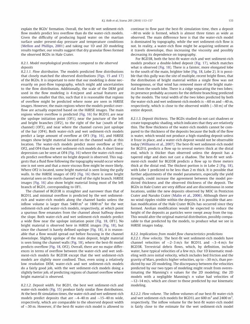
explain the BGDs’ formation. Overall, the best-fit wet sediment-richflow models predict less overflow than do the water-rich models.Given the difficulty of producing liquid water on the martiansurface under present-day pressure and temperature conditions(Mellon and Phillips, 2001) and taking our 1D and 2D modelingresults together, our results suggest that dry granular flows formedthe observed BGDs in Hale Crater.

8.2.1. Model morphological predictions compared to the observeddeposits8.2.1.1. Flow distribution. The models predicted flow distributionsthat closely matched the observed distributions (Figs. 15 and 17)of the BGDs. It is important to note that our modeling is done nec-essarily on post-flow topography, which might add uncertaintiesto the flow distribution. Additionally, the scale of the DEM gridused in the flow modeling is 4 m/post and actual features aresometimes smaller that this, such that it is reasonable that regionsof overflow might be predicted where none are seen in HiRISEimages. However, the main regions where the models predict over-flow are actually expected based on the HiRISE images. The mainregions where overflow is predicted (Fig. 16) for BGD1L are nearthe upslope initiation point (OF1), near the juncture of the leftand bright branches (OF2), to the right of the bar (south of thechannel) (OF3), and near where the channel curves just upslopeof the bar (OF4). Both water-rich and wet sediment-rich modelspredict a large amount of overflow at OF3 (Fig. 16), and HiRISEimages show bright material located on the channel walls at thislocation. The water-rich models predict more overflow at OF1,OF2, and OF4 than the wet sediment-rich models do. A short lineardepression can be seen at OF4 (Fig. 16) where the water-rich mod-els predict overflow where no bright deposit is observed. This sug-gests that a fluid flow following the topography would occur whereone is not seen and that a more viscous flow might be more likely.Where OF2 is located, some bright material is seen lining the gullywalls. In the HiRISE images of OF2 (Fig. 16) there is some brightmaterial seen on the north channel wall of the right branch. HiRISEimages (Fig. 16) also show bright material lining most of the leftbranch of BGD1, corresponding to OF1.

The channel of BGD3R is straighter and narrower than that ofBGD1L and minimal overflow is predicted by the wet sediment-rich and water-rich models along the channel banks unless theinflow volume is larger than 5400 m3 or 1800 m3 for the wetsediment-rich and water-rich models, respectively, at which pointa spurious flow emanates from the channel about halfway downthe slope. Both water-rich and wet sediment-rich models predicta wide flow near the upslope initiation point (Fig. 18, OF1). Nobright material is observed here in HiRISE images (Fig. 18), butsince the channel is barely defined upslope (Fig. 18), it is reason-able that a flow would spread out before focusing in the channeldownslope. Slightly upslope of the main deposit, bright materialis seen lining the channel walls (Fig. 18), where the best-fit modelpredicts overflow (Fig. 18, OF2). Overall, there are no major differ-ences in terms of overflow between the water-rich and wet sedi-ment-rich models for BGD3R except that the wet sediment-richmodels are slightly more confined. Thus, even using a relativelylow resolution DEM, water-rich and wet sediment-rich modelsdo a fairly good job, with the wet sediment-rich models doing aslightly better job, of predicting regions of channel overflow wherebright material is observed.

8.2.1.2. Deposit width. For BGD1, the best wet sediment-rich andwater-rich models (Fig. 15) produce fairly similar flow distributions.At the best-fit simulation times, the water-rich andwet sediment-richmodels predict deposits that are �4–40 m and �15–40 m wide,respectively, which are comparable to the observed deposit widthof �30 m. However, if the best-fit water-rich model is allowed to

continue to flow past the best-fit simulation time, then a deposit�80 m wide is formed, which is almost three times as wide asobserved. The main difference here is that the water-rich modelis dominated by topography, while the wet sediment-rich flow isnot. In reality, a water-rich flow might be acquiring sediment asit travels downslope, thus increasing the viscosity and possiblydecreasing its dependence on topography.

For BGD3R, both the best-fit water-rich and wet sediment-richmodels produce a double-lobed deposit (Fig. 17), which matcheswhat is observed (Fig. 18). There is a fainter, more elongated lobeto the south of the main, brighter lobe (Fig. 18, Lobe 2). It is possi-ble that this gully was the site of multiple, recent bright flows, thatthe distribution of bright material within a single flow was nothomogenous, or that wind has removed more of the bright mate-rial from the south lobe. There is a ridge separating the two lobes;its presence probably accounts for the definite branching predictedby the models. The total width of the two lobes predicted by boththe water-rich and wet sediment-rich models is �60 m and �40 m,respectively, which is close to the observed width (�50 m) of theentire deposit.

8.2.1.3. Deposit thickness. The BGDs studied do not cast shadows orcreate topographic shading, which indicates that they are relativelythin. The flow thickness of the water-rich models cannot be com-pared to the thickness of the deposits because the bulk of the flowis water, which would not produce a high-standing deposit unlessit froze in place, and a water-rich deposit would not be observabletoday (Williams et al., 2007). The best-fit wet sediment-rich modelfor BGD1L predicts a flow up to several meters thick at the distalend, which is thicker than observed unless the deposit has atapered edge and does not cast a shadow. The best-fit wet sedi-ment-rich model for BGD3R predicts a flow up to three metersthick at the distal end. The thickest portion is in Lobe 2 (Fig. 18),with Lobe 1 predicted to be less than 2 m thick. It is possible thatfurther adjustments of the model parameters, especially the yieldstrength, could increase the agreement between the model pre-dicted thickness and the observed thickness of the deposit. TheBGDs in Hale Crater are very diffuse and are discontinuous in somelocations, unlike the new deposits observed by MOC in PentictonCrater and Naruko Crater (Malin et al., 2006). Although there areno wind ripples visible within the deposits, it is possible that aeo-lian modification of the Hale Crater BGDs has occurred since theyformed. Aeolian modification would be expected to reduce theheight of the deposits as particles were swept away from the top.This would alter the original material distribution, possibly compa-rable to that predicted by the models, to produce what we see inHiRISE images today.

8.2.2. Implications from model flow characteristics predictions8.2.2.1. Flow velocity. The best-fit wet sediment-rich models havechannel velocities of �2–3 m/s for BGD1L and �3–4 m/s forBGD3R. Terrestrial debris flows, which, by definition, includewater, have typical velocities of a few m/s. Our 1D kinematic mod-eling with zero initial velocity, which includes bed friction and thegravity of Mars, predicts higher velocities, up to �30 m/s, than pre-dicted by our 2D modeling. The discrepancy between the velocitiespredicted by our two types of modeling might result from overes-timating the Manning’s n values for the 2D modeling; the 2Dmodels with a negligible Manning’s n value had velocities of�12–14 m/s, which are closer to those predicted by our kinematicmodeling.

8.2.2.2. Flow volume. The inflow volumes of our best-fit water-richand wet sediment-rich models for BGD1L are 600 m3 and 2400 m3,respectively. The inflow volume for the best-fit water-rich modelis fairly close to the estimate for the wet sediment-rich model


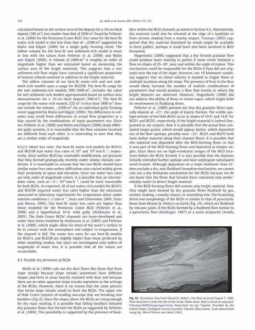
calculated based on the surface area of the deposit for a 10 cm thickdeposit (385m3), but smaller than that of 2500m3 found by Pelletieret al. (2008) for the Penticton Crater BGD. Our value for the best-fitwater-rich model is also less than that of �2500 m3 suggested byMalin and Edgett (2000) for a single gully forming event. Theinflow volume for the best-fit wet sediment-rich model is morein line with the values from Pelletier et al. (2008) and Malinand Edgett (2000). A volume of 2400 m3 is roughly an order ofmagnitude higher than we estimated based on measuring thesurface area of the bright materials. This suggests that a wetsediment-rich flow might have contained a significant proportionof neutral colored material in addition to the bright material.

The inflow volumes of our best-fit water-rich and wet sedi-ment-rich models span a range for BGD3R. The best-fit range forthe wet sediment-rich models, 900–5400 m3, includes the valuefor wet sediment-rich models approximated based on surface areameasurements for a 10 cm thick deposit (940 m3). The best-fitrange for the water-rich models, 525 m3 to less than 1800 m3 doesnot include the volume, �2500 m3, for an individual gully formingevent suggested by Malin and Edgett (2000). The differences in vol-umes may result from differences in actual flow properties or abias caused by the combinations of input parameters run. Sincewe, Pelletier et al. (2008) and Malin and Edgett (2000) study differ-ent gully systems, it is reasonable that the flow volumes involvedare different from each other. It is interesting to note that theyare a similar order of magnitude.

8.2.2.3. Water loss rates. Our best-fit water-rich models for BGD1Land BGD3R had water loss rates of 104 and 105 mm h�1, respec-tively. Since neither BGD has resolvable modification, we presumethat they formed geologically recently under similar climatic con-ditions. It is reasonable to assume that the two BGDs should havesimilar water loss rates unless infiltration rates varied widely giventheir proximity in space and elevation. Since our water loss ratesare only order of magnitude values, it is possible that an interme-diate value, such as �5 � 104 mm h�1, could be most reasonablefor both BGDs. As expected, all of our water-rich models for BGD1Land BGD3R required water loss rates higher than the minimummeasured in laboratory experiments for evaporation alone undermartian conditions (�1 mm h�1, Sears and Chittenden, 2005; Searsand Moore, 2005). Our best-fit water loss rates are higher thanthose modeled for the Penticton Crater BGD (Pelletier et al.,2008) and a hypothetical 10 m wide gully (Heldmann et al.,2005). The Hale Crater BGDs’ channels are more-developed andwider than those modeled by Heldmann et al. (2005) and Pelletieret al. (2008), which might allow for more of the water’s surface tobe in contact with the atmosphere and subject to evaporation, ifthe channel is full. The water loss rates for our best-fit modelsfor BGD1L and BGD3R are slightly higher than those predicted byother modeling studies, but since we investigated only orders ofmagnitude of water loss, it is possible that all the values arereconcilable.

8.3. Possible dry formation of BGDs

Malin et al. (2006) rule out dry dust flows like those that formslope streaks because slope streaks sometimes have differentshapes and form in areas heavily mantled with dust and becausethere are no other apparent slope streaks anywhere in the settingsof the BGDs. However, there is no reason that the same processthat forms slope streaks needs to form the BGDs. The upper rimof Hale Crater consists of eroding outcrops that are breaking intoboulders (Fig. 6). Since the slopes above the BGDs are steep enoughfor dry mass wasting, it is possible that falling boulders initiateddry granular flows that formed the BGDs as suggested by Pelletieret al. (2008). This possibility is supported by the presence of boul-

ders within the BGD channels as noted in Section 4.2. Alternatively,dry material could also be released at the edge of a landslide orfrom seismic shaking from a nearby impact. Treiman (2003) sug-gested that dry material deposited by winds might be availableto form gullies; perhaps it could have also been involved in BGDformation.

Hugenholtz (2008) suggested that a dry frosted granular flowcould produce mass wasting in gullies if some event initiated aflow on slopes of 25–30�, near and within the angle of repose. Thismechanism could be responsible for the BGDs if they did not orig-inate near the top of the slope; however, our 1D kinematic model-ing suggests that no initial velocity is needed to trigger flows atmultiple locations along the slope. The presence of frost in the flowwould likely increase the number of realistic combinations ofparameters that would produce a flow that travels to where thebright deposits are observed. However, Hugenholtz (2008) didnot address the ability of flows to retain vapor, which might limitits involvement in fluidizing flows.

Pelletier et al. (2008) pointed out that dry granular flows typi-cally deposit at �21�, the angle of kinetic friction. The visible ups-lope extents of the Hale BGDs occur at slopes of 10.4� and 14.8� forBGD1 and BGD3, respectively. If the bright material is indeed fine-grained as we suspect, then it is possible that the actual flow con-tained larger grains, which would appear darker, which depositedout of the flow upslope, possibly near �21�. BGD1 and BGD3 bothhave darker material along their channel floors. It is possible thatthis material was deposited after the BGD-forming flows or thatit was part of the BGD-forming flows and deposited at steeper an-gles. Since there are no high-resolution images of the BGD loca-tions before the BGDs formed, it is also possible that the depositsinitially extended further upslope and have undergone subsequentwind erosion. Although deposition on a slope shallower than 21�does exclude a dry, non-fluidized formation mechanism, we cannotrule out a dry formation mechanism for the BGDs because we donot know that the flows that formed them contained only prefer-entially easier to detect bright material.

If the BGD-forming flows did contain only bright material, thenthey might have formed by dry granular flows fluidized by gas,seismic shaking, a nearby impact, or something else. The branchingdistal end morphology of the BGDs is similar to that of pyroclasticflows fromMount St. Helen’s on Earth (Fig. 19), which are fluidizedby volcanic gases. If the BGDs formed by a fluidized flow similar toa pyroclastic flow (Denlinger, 1987) or a snow avalanche (Sovilla

Fig. 19. Pyroclastic flow from Mount St. Helen’s. The flow occurred August 7, 1980.Flow direction is from the left of the scene. Photo from: http://vulcan.wr.usgs.gov/Volcanoes/MSH/Images/pyroclastic_flows.html by Lyn Topinka. Provided by theUnited States Geological Survey/Cascades Volcano Observatory. Scale determinedusing Fig. 298 of Wilson and Head (1981).


and Bartelt, 2002), then the presence of the bright material seenlining the channels of the BGDs (Fig. 8) could be explained bylofted dust that is typical of these types of flows. It is interestingto note that bright flows on ungullied slopes (Fig. 20) have alsobeen observed, which supports our suggestion that the BGDsmay not be genetically related to the gullies, but only BGDs associ-ated with gullies are, to date, known to be very recently active frombefore-and-after images.

Heldmann et al. (2008a) suggested that mudflows, requiring li-quid water, formed the bright deposits based on a rain-inducedterrestrial analog in the Atacama Desert. They did not propose asource of the liquid water required distinct from those suggestedfor gullies. They also did not comment on the different slope con-ditions at the two locations; the Atacama deposit appears to be ona very shallow slope, while the BGDs are found below steep slopes.If water was involved in the formation of the Hale Crater BGDs,then the bright deposits represent a location of current or very re-cent water. However, because of the steep nature of the slopes,there is no conclusive evidence that the bright deposits are formedby recently flowing surficial water (McEwen et al., 2007a; Pelletieret al., 2008). Our 1D kinematic modeling shows that dry granularflows with zero initial velocity and a range of parameters couldflow out approximately as far as the deposits are observed. Weare unable to rule out muddy flows, but given the difficulty of pro-ducing significant quantities of liquid water on the martian surfacetoday (Mellon and Phillips, 2001) and the fact that the BGDs areobserved at locations with steep upslope regions, the results of thisstudy support the likelihood that the Hale Crater BGDs, similar tothe Penticton Crater BGD (Pelletier et al., 2008), were formed bydry granular flows.

9. Summary and conclusions

The BGDs are probably bright due to the redeposition of pre-existing bright material, which consists of fine-grained particles(McEwen et al., 2007a). Based on our color analysis, the materialscomprising the bright deposits may not have a different composi-tion from surrounding material but likely differ in grain size. This isconsistent with CRISM results (Supporting Online Material, McEwenet al., 2007a; Barnouin-Jha et al., 2008). The existence of brightlayers upslope and bright material lining the gully channel wallsprovides a source for the bright material. Even though the BGDsstart midslope, they could have been transported from the top ofthe slope with deposition beginning when the slope falls belowthe angle of kinetic friction, �21�, or when the supply of a trans-

porting fluid diminishes enough to start depositing transportedsediment. Fine dust, which appears bright, could easily be depos-ited from the atmosphere, possibly forming agglomerates thatare transported as or by a flow. It is possible that the bright mate-rials were bleached by water or contain evaporites, althoughCRISM has not yet detected the latter. The multitemporal imagestudy did not find any significant changes in the deposits’ shapes,which reaffirms that the deposits are not likely composed of waterice or frost (Williams et al., 2007). The fact that the Hale CraterBGDs have rather diffuse ends suggests that aeolian processesmight have acted on them since or during their formation. HiRISEimage ESP_011819_1445, acquired approximately one martianyear after PSP_002932_1445 and PSP_3209_1445 at the same loca-tion, shows no visible changes in the deposits’ tone or shape. FutureHiRISE images at complementary seasons might allow for tonechange detection.

The question about whether all the recent bright deposits wereformed by wet or dry flows remains; however, these analyses sug-gest that pronouncement of definitive evidence of recent liquidwater on Mars (Malin et al., 2006) was premature. Given thelengthy nature of the DEM development and modeling processes,it is necessary to focus future efforts on the best candidate BGDsfor liquid water involvement with the overall goal being to dis-cover if formation of any of the recent BGDs cannot be explainedby a dry granular flow. Our results suggest that the BGD-formingflows were likely dry flows initiated by a rockfall in steep regionsupslope of the BGDs and consisting of fine-grained particles, possi-bly clumped together, as well as other materials.

Acknowledgments

The authors wish to acknowledge Oded Aharonson’s group atCaltech for producing the DEM used in this study and the HiRISEand MRO teams for useful discussions and advice. KJK and ASMwould like to acknowledge support from the HiRISE (on theMRO) Grant (JPL Subcontract #1272218) and a NASA MDAP Grant# NNX08AL08G. We would like to thank an anonymous reviewer,Allan Treiman, and Laszlo Keszthelyi for helpful reviews thatgreatly improved this manuscript.

Appendix A. Supplementary material

Supplementary data associated with this article can be found, inthe online version, at doi:10.1016/j.icarus.2009.09.009.

References

Albee, A.L., Palluconi, F.D., Arvidson, R.E., 1998. Mars global surveyor mission:Overview and status. Science 279, 1671–1672. doi:10.1126/science.279.5357.1671.

Anderson, J.A., Sides, S.C., Soltesz, D.L., Sucharski, T.L., Becker, K.J., 2004.Modernization of the integrated software for imagers and spectrometers.Lunar Planet. Sci. 35. <http://www.lpi.usra.edu/meetings/lpsc2004/pdf/2039.pdf>(Abstract 2039).

Andrews-Hanna, J.C., Zuber, M.T., Banerdt, W.B., 2008. The Borealis basin and theorigin of the martian crustal dichotomy. Nature 453, 1212–1215. doi:10.1038/nature07011.

Barnouin-Jha, O.S., McGovern, A., Buczkowski, D., Seelos, K., Seelos, F., Murchie, S.,Ehlmann, B., 2008. Martian gullies as seen by the Compact ReconnaissanceImaging Spectrometer for Mars (CRISM). Fall AGU Meeting. <http://adsabs.harvard.edu/abs/2008AGUFM.P32B..04B> (Abstract 8380).

Bart, G.D., 2007. Comparison of small lunar landslides and martian gullies. Icarus187 (2), 417–421. doi:10.1016/j.icarus.2006.11.004.

Cabrol, N.A., Wynn-Williams, D.D., Crawford, D.A., Grin, E.A., 2001. Recent aqueousenvironments in martian impact craters: An astrobiological perspective. Icarus154 (1), 98–112. doi:10.1006/icar.2001.6661.

Christensen, P.R., 2003. Formation of recent martian gullies through melting ofextensive water-rich snow deposits. Nature 422, 45–48. doi:10.1038/nature01436.

Fig. 20. Bright deposits without gullies. These bright deposits are located in BahramVallis. Note that these deposits are modified and cover most of their host slopes,unlike the BGDs. They are very thin deposits based on the fact that they do not castshadows. HiRISE image PSP_003671_2010, equirectangular projection centered at20.6�N, 303�E, 0.282 m/pixel.


Costard, F., Forget, F., Mangold, N., Peulvast, J.P., 2002. Formation of recent martiandebris flows by melting of near-surface ground ice at high obliquity. Science295, 110–113. doi:10.1126/science.1066698.

Delamare, W.A., and 13 colleagues, 2009. Color imaging of Mars by the HighResolution Imaging Science Experiment (HiRISE). Icarus, 205, 38–52.

Denlinger, R.P., 1987. A model for generation of ash clouds by pyroclastic flows,with application to the 1980 eruptions at Mount St. Helens, Washington. J.Geophys. Res. 92 (B10), 10284–10298. doi:10.1029/JB092iB10p10284.

Dickson, J.L., Head, J.W., 2005. Detection of gullies on central peaks and crater rimson Mars: implications for the origin of gullies. Lunar Planet. Sci. 36. <http://www.lpi.usra.edu/meetings/lpsc2005/pdf/1097.pdf> (Abstract 1097).

Dickson, J.L., Head, J.W., Kreslavsky, M., 2007. Martian gullies in the southern mid-latitudes of Mars: Evidence for climate-controlled formation of young fluvialfeatures based upon local and global topography. Icarus 188 (2), 315–323.doi:10.1016/j.icarus.2006.11.020.

FLO Engineering, Inc., 2006. FLO-2D User Manual, Version 2006.1. Nutrioso, Arizona.<http://www.flo-2d.com/v2006/Documentation/Manual_Main_2006.pdf>.

Gaidos, E.J., 2001. Note: Cryovolcanism and the recent flow of liquid water on Mars.Icarus 153 (1), 218–223. doi:10.1006/icar.2001.6649.

Gilmore, M.S., Phillips, E.L., 2002. Role of aquicludes in formation of martian gullies.Geology 30 (12), 1107–1110. doi:10.1130/0091-7613(2002)030.

Golombek, M.P., and 54 colleagues, 1999. Overview of the Mars Pathfinder mission:Launch through landing, surface operations, data sets, and science results. J.Geophys. Res. 104 (E4), 8523–8554. doi:10.1029/98JE02554.

Gulick, V.C., McEwen, A.S., 2007. Early HiRISE observations of fluvial andhydrothermal features. Lunar Planet. Sci. 38. <http://www.lpi.usra.edu/meetings/lpsc2007/pdf/2300.pdf> (Abstract 1338).

Gulick, V.C., Davatzes, A., Kolb, K., and the HiRISE Team, 2007. Some insights ongully morphology and formation on Mars from HiRISE. In: Seventh InternationalConference on Mars. <http://www.lpi.usra.edu/meetings/7thmars2007/pdf/3371.pdf> (Abstract 3371).

Gulick, V.C., and the HiRISE Team, 2008. A closer look at valley, channel and gullyformation on Mars with HiRISE. Lunar Planet. Sci. 39. <http://www.lpi.usra.edu/meetings/lpsc2008/pdf/2411.pdf> (Abstract 2411).

Hartmann, W.K., Thorsteinsson, T., Sigurdsson, F., 2003. Martian hillside gullies andicelandic analogs. Icarus 162 (2), 259–277. doi:10.1016/S0019-1035(02)00065-9.

Hecht, M.H., 2002. Metastability of liquid water on Mars. Icarus 156, 373–386.doi:10.1006/icar.2001.6794.

Heldmann, J.L., Conley, C., Brown, A.J., Fletcher, L., 2008a. Atacama Desert mudflowas an analog for recent gully activity on Mars. In: Workshop on Martian Gullies.<http://www.lpi.usra.edu/meetings/gullies2008/pdf/8017.pdf> (Abstract 8017).

Heldmann, J.L., Edgett, K.S., Toon, O.B., Mellon, M.T., 2008b. Martian gullies: Varietyof settings and implications for formation processes. In: Workshop on MartianGullies. <http://www.lpi.usra.edu/meetings/gullies2008/pdf/8031.pdf>(Abstract 8031).

Heldmann, J.L., Mellon, M.T., 2004. Observations of martian gullies and constraintson potential formation mechanisms. Icarus 168 (2), 285–304. doi:10.1016/j.icarus.2003.11.024.

Heldmann, J.L., Toon, O.B., Pollard, W.H., Mellon, M.T., Pitlick, J., McKay, C.P.,Andersen, D.T., 2005. Formation of martian gullies by the action of liquid waterflowing under current martian environmental conditions. J. Geophys. Res. 110(E5), E05004. doi:10.1029/2004JE002261.

Heldmann, J.L., Carlsson, E., Johansson, H., Mellon, M.T., Toon, O.B., 2007.Observations of martian gullies and constraints on potential formationmechanisms II. The northern hemisphere. Icarus 188 (2), 324–344.doi:10.1016/j.icarus.2006.12.010.

Hoffman, N., 2002. Active polar gullies on Mars and the role of carbon dioxide.Astrobiology 2 (3), 313–323. doi:10.1089/153110702762027899.

Hugenholtz, C.H., 2008. Frosted granular flow: A new hypothesis for mass wastingin martian gullies. Icarus 197 (1), 65–72. doi:10.1016/j.icarus.2008.04.010.

Ishii, T., Miyamoto, H., Sasaki, S., Tajika, E., 2006. Constraints on the formation ofgullies on Mars: A possibility of formation of gullies by avalanches of granularCO2 Ice particles. Lunar Planet. Sci. 37. <http://www.lpi.usra.edu/meetings/lpsc2006/pdf/1646.pdf> (Abstract 1646).

Jop, P., Forterre, Y., Pouliquen, O., 2005. Crucial role of sidewalls in granular surfaceflows: Consequences for the rheology. J. Fluid Mech. 541, 167–192. doi:10.1017/S0022112005005987.

Jop, P., Forterre, Y., Pouliquen, O., 2006. A constitutive law for dense granular flows.Nature 441, 727–730. doi:10.0138/nature04801.

Kirk, R.L., and 18 colleagues, 2008. Ultrahigh resolution topographic mapping ofMars with MRO HiRISE stereo images: Meter-scale slopes of candidate Phoenixlanding sites. J. Geophys. Res. 113 (E12), E00A24. doi:10.1029/2007JE003000.

Knauth, L.P., Burt, D.M., 2002. NOTE eutectic brines on Mars: Origin and possiblerelation to young seepage features. Icarus 158 (1), 267–271. doi:10.1006/icar.2002.6866.

Kolb, K.J., McEwen, A.S., Gulick, V.C., and the HiRISE Team, 2007. Bright gullydeposits: Geological and topographical settings. In: Seventh InternationalConference on Mars. <http://www.lpi.usra.edu/meetings/7thmars2007/pdf/3245.pdf> (Abstract 1353).

Kolb, K.J., Okubo, C.H., 2009. Coregistration of Mars Orbiter Laser Altimeter (MOLA)topography with high-resolution Mars images. Comput. Geosci., in press.doi:10.1016/j.cageo.2009.04.008.

Lanza, N.L., Gilmore, M.S., 2006. Depths, orientations and slopes of martian hillsidegullies in the northern hemisphere. Lunar Planet. Sci. 37. <http://www.lpi.usra.edu/meetings/lpsc2006/pdf/2412.pdf> (Abstract 2412).

Lee, P., Cockell, C.S., Marinova, M.M., McKay, C.P., Rice Jr., J.W., 2001. Snow and icemelt flow features on Devon Island, Nunavut, Arctic Canada as possible analogsfor recent slope flow features on Mars. Lunar Planet. Sci. 32. <http://www.lpi.usra.edu/meetings/lpsc2001/pdf/1809.pdf> (Abstract 1809).

Lin, M.-L., Wang, K.-L., Huang, J.-J., 2005. Debris flow run off simulation andverification – Case study of Chen-You-Lan Watershed, Taiwan. Nat. HazardsEarth Syst. Sci. 5, 439–445.

Malin,M.C., and13 colleagues, 2007. Context Camera Investigation onboard theMarsReconnaissance Orbiter. J. Geophys. Res. 112 (E5). doi:10.0129/2006JE002808.

Malin, M.C., Edgett, K.S., 2000. Evidence for recent groundwater seepage and surfacerunoff on Mars. Science 288, 2330–2335. doi:10.1126/science.288.5475.2330.

Malin, M.C., Edgett, K.S., 2001. Mars global surveyor Mars orbiter camera:Interplanetary cruise through primary mission. J. Geophys. Res. 106 (E10),23429–23570. doi:10.1029/2000JE001455.

Malin, M.C., Edgett, K.S., Posiolova, L.V., McCauley, S.M., Noe Dobrea, E.Z., 2006.Present-day impact cratering rate and contemporary gully activity on Mars.Science 314, 1573–1577. doi:10.1126/science.1135156.

McClung, D., Schaerer, P., 2006. The Avalanche Handbook, third ed. TheMountaineers Books, Seattle, p. 87.

McEwen, A.S., and 32 colleagues, 2007a. A closer look at water-related geologicactivity on Mars. Science 317, 1706–1709. doi:10.1126/science.1143987.

McEwen, A.S., and 14 colleagues, 2007b. Mars Reconnaissance Orbiter’s HighResolution Imaging Science Experiment (HiRISE). J. Geophys. Res. 112 (E05),E0505S02. doi:10.1029/2005JE002605.

McMahon, S.K., 1996. Overview of the planetary data system. Planet. Space Sci. 44(1), 3–12.

Mellon, M.T., 1997. Small-scale polygonal features on Mars: Seasonal thermalcontraction cracks in permafrost. J. Geophys. Res. 102 (E11), 25617–25638.doi:10.1029/97JE02582.

Mellon, M.T., Phillips, R.J., 2001. Recent gullies on Mars and the source of liquidwater. J. Geophys. Res. 106 (E10), 23165–23180. doi:10.1029/2000JE001424.

Mikos, M., Fazarinc, R., Majes, B., Rajar, R., Zagar, D., Krzyk, M., Hojnik, T., Cetina, M.,2006. Numerical simulation of debris flows triggered from the Strug rock fallsource area, W Slovenia. Nat. Hazards Earth Syst. Sci. 6 (2), 261–270.

Moore, H.J., Jakosky, B.M., 1989. Viking landing sites, remote-sensing observations,and physical properties of martian surface materials. Icarus 81, 164–184.doi:10.1016/0019-1035(89)90132-2.

Moore, S.R., Sears, D.W.G., 2006. On laboratory simulation and the effect of smalltemperature oscillations about the freezing point and ice formation on theevaporation rate of water on Mars. Astrobiology 6 (4), 644–650. doi:10.1089/ast.2006.6.644.

Murchie, S., and 49 colleagues, 2007. Compact Reconnaissance ImagingSpectrometer for Mars (CRISM) on Mars Reconnaissance Orbiter (MRO). J.Geophys. Res. 112 (E5). doi:10.1029/2006JE002682.

Musselwhite, D.S., Swindle, T.D., Lunine, J.I., 2001. Liquid CO2 breakout and theformation of recent small gullies on Mars. Geophys. Res. Lett. 28 (7), 1283–1285. doi:10.1029/2000GL012496.

Neumann, G.A., Rowlands, D.D., Lemoine, F.G., Smith, D.E., Zuber, M.T., 2001.Crossover analysis of Mars Orbiter Laser Altimeter data. J. Geophys. Res. 106(E10), 23753–23768. doi:10.1029/2000JE001381.

Nicholson, P., 1838. Practical Masonry, Bricklaying and Plastering, both Plain andOrnamental. Thomas Kelly, London, p. 36.

Nimmo, F., 2002. Admittance estimates of mean crustal thickness and density of themartian hemispheric dichotomy. J. Geophys. Res. 107 (E11). doi:10.1029/2000JE001488.

O’Brien, J.S., Julien, P.Y., Fullerton, W.T., 1993. Two-dimensional water flood andmudflow simulation. J. Hydraulic Eng. 119 (2), 244–261. doi:10.1061/(ASCE)0733-9429(1993)119:2(244).

Parsons, R.A., Kreslavsky, M.A., Nimmo, F., 2008. Martian gully slope measurementsmade using HiRISE stereo pairs. Lunar Planet. Sci. 39. <http://www.lpi.usra.edu/meetings/lpsc2008/pdf/2328.pdf> (Abstract 2328).

Pelletier, J.D., Kolb, K.J., McEwen, A.S., Kirk, R.L., 2008. Recent bright gully depositson Mars: Wet or dry flow? Geology 36, 211–214. doi:10.1130/G24346A.1.

Pirulli, M., Sorbino, G., 2008. Assessing potential debris flow runout: A comparisonof two simulation models. Nat. Hazards Earth Syst. Sci. 8, 961–971.

Pouliquen, O., 1999. Scaling laws in granular flows down rough inclined planes.Phys. Fluids 11 (3), 542–548. doi:10.1063/1.869928.

Sears, D.W.G., Chittenden, J.D., 2005. On laboratory simulation and the temperaturedependence of the evaporation rate of brine on Mars. Geophys. Res. Lett. 32(23), L23203. doi:10.1029/2005GL024154.

Sears, D.W.G., Moore, S.R., 2005. On laboratory simulation and the evaporation rateof water on Mars. Geophys. Res. Lett. 32 (16), L16202. doi:10.1029/2005GL023443.

Smith, D., Neumann, G., Ford, P., Arvidson, R.E., Guinness, E.A., Slavney, S., 1998.Mars global surveyor laser altimeter precision experiment data record. NASAPlanetary Data System, MGS-M-MOLA-3-PEDR-L1A-V1.0.

Sovilla, B., Bartelt, P., 2002. Observations and modeling of snow avalancheentrainment. Nat. Hazards Earth Syst. Sci. 2 (3/4), 169–179.

Squyres, S.W., and 49 colleagues, 2004a. The Opportunity Rover’s Athena scienceinvestigation at Meridiani Planum, Mars. Science 306, 1698–1703. doi:10.1126/science.1106171.

Squyres, S.W., and 49 colleagues, 2004b. The Spirit Rover’s Athena science inves-tigation at Gusev Crater, Mars. Science 305, 794–800. doi:10.1126/science.1100194.

Stewart, S.T., Nimmo, F., 2002. Surface runoff features on Mars: Testing the carbondioxide formation hypothesis. J. Geophys. Res. 107 (E9), 5069–5080.doi:10.1019/2000JE001465.


Supharatid, S., 2006. The Hat Yai 2000 flood: The worst flood in Thai history. Hydrol.Process. 20 (2), 307–318. doi:10.1002/hyp.5912.

Tornabene, L.L., McEwen, A.S., and the HiRISE Team, 2008. Recent channel systemsemanating from Hale Crater ejecta: Implications for the Noachian landscapeevolution of Mars. Lunar Planet. Sci. 39. <http://www.lpi.usra.edu/meetings/lpsc2008/pdf/2180.pdf> (Abstract 2180).

Treiman, A.H., 2003. Geologic settings of martian gullies: Implications fortheir origins. J. Geophys. Res. 108 (E4), 8031–8043. doi:10.1029/2002JE001900.

Urquhart, M.L., Gulick, V.C., 2003. Plausibility of the ‘‘White Mars” hypothesis basedupon the thermal nature of the martian subsurface. Geophys. Res. Lett. 30 (12),1–24. doi:10.1029/2002GL016158.

Williams, K.E., Toon, O.B., Heldmann, J., 2007. Modeling water ice lifetimes at recentmartian gully locations. Geophys. Res. Lett. 34 (9), L09204. doi:10.1029/2007GL029507.

Wilson, H.M., 1900. A dictionary of topographic forms. J. Am. Geogr. Soc. NY 32 (1),36–39.

Wilson, L., Ghatan, G.J., Head, J.W., Mitchell, K.L., 2004. Mars outflow channels: Areappraisal of the estimation of water flow velocities from water depths,regional slopes, and channel floor properties. J. Geophys. Res. 109 (E9).doi:10.1029/2004JE002281.

Wilson, L., Head, J.W., 1981. Morphology and rheology of pyroclastic flows and theirdeposits, and guidelines for future observations. US Geological SurveyProfessional Paper 1250, pp. 513–524.

Wray, J.J., Ehlmann, B.L., Squyres, S.W., Mustard, J.F., Kirk, R.L., 2008. Compositionalstratigraphy of clay-bearing layered deposits at Mawrth Vallis, Mars. Geophys.Res. Lett. 35 (12), L12202. doi:10.1029/2008GL034385.

Zuber, M.T., Smith, D.H., Solomon, S.C., Muhleman, D.O., Head, J.W., Garvin, J.B.,Abshire, J.B., Bufton, J.L., 1992. The Mars observer laser altimeter investigation. J.Geophys. Res. 97 (E5), 7781–7797 (92JE00341).


Documents

Modeling the formation of bright slope deposits associated