Modeling the Magnetron Toy

Chris DuBois

May 9, 2005

Abstract

Many real-world phenomena are often too complex for us to capture entirely using mathematicaltools, but a careful approach enables an exploration of that complexity and may provide insight intothe phenomena. The author found a simple desk toy, the “Magnetron,” to be a perfect target forexploration: while simply designed and constructed, one quickly realizes the system has very complexdynamics. The toy features two rotors, spaced slightly apart, with magnets mounted at the end ofeach arm; manually spinning one rotor causes the other rotor to spin due to the interactions betweenthe magnetic fields. In this paper we present a mathematical model that successfully reproducesseveral of the toy’s behaviors. In the future we hope to explore the transitions between variousequilibria of the system.

The Magnetron

The Magnetron toy has two plastic rotors mounted on a wooden block by metal spindles that serveas axles. Each rotor has three evenly spaced arms. At the end of each arm, there is a small barmagnet mounted inside a plastic housing with its North pole oriented away from the rotor center.The two rotors are spaced such that they nearly touch when they are closest to each other. Sincedipoles are subject to forces due to external magnetic fields, the fields produced by the magnets inone rotor affect the rotation of the opposite rotor and vice versa.

Introduction

There are several interesting aspects of this physical system that become apparent after a week-longobsession with this toy. First, the system has a stable equilibrium when two arms are pointingtowards the middle but not directly at each other. This can be explained by the magnets wantingto align themselves in the other magnet’s field. The system has two unstable equilibria: when therotor arms are as far away from each other as possible and when two arms are positioned directlytowards each other. Additionally, there is a steady state when one rotor is moving fast and the otheris such that one arm points directly away from the system center.

Aside from equilibria, the toy shows some cool behavior such as “momentum transfer” - whereone rotor begins with high angular velocity but suddenly stops while the second rotor begins fastrotation from a standstill. It is quite fascinating to watch how the two transfer energy to each otherso efficiently without physically touching. Another neat effect is “velocity matching,” where the tworotors are spinning in opposite directions such that they keep a nearly constant velocity. Also, thereis a bouncing effect that is important for understanding the system since it often happens when thesystem is winding down to equilibrium.

To the author’s knowledge, there is only one other attempt at modeling this particular system [1].Whereas this paper also models the magnets as point dipoles, I use the system’s potential energyto find the equations of motion instead of calculating the individual forces present. This modelimproves on previous models by incorporating a frictional force (and by successfully modeling thedynamics of the toy!).

1

Assumptions of The Model

2 Dimensional

Because of the way the two rotors are mounted, rotational motion is restricted a single plane parallelto the base plate. Also, the magnetic fields in the vertical direction are symmetric with respect tothis plane, so they do not play an important role in the dynamics of the two rotors. Both of theseconsiderations make a 2D model reasonable.

Energy

We consider the total energy of the system to be the sum of the kinetic and potential energy. Usingfundamental Newtonian principles, we calculate the rotational kinetic energy from the inertia andangular velocity of each rotor. Using equations from electromagnetic theory, we can calculate thepotential energy present from the interacting magnetic fields of the dipoles. Approaching the stateof the system in terms of total energy allows us to use a Lagrangian formulation of the model todescribe the progression of the system.

Rotational Friction

We make the assumption that the axle provides a rotational frictional force on the rotors that isproportional to each rotor’s angular velocity. Since it is impossible that both axles act upon therotors in exactly the same amount, the coefficient of friction must be slightly different for each rotor.Employing a rotational drag term is a reasonable choice since it is impossible for the axles to beperfectly frictionless and an important choice since it provides an avenue for energy loss. (We knowthe toy exhibits energy loss since, in practice, the two rotors eventually find a stable, motionlessequilibrium after initially having angular velocity.)

Higher Order Frictions

We ignore the effects of air resistance and other higher order drags to clarify the effects of thefirst order terms. And after considering the geometry of the rotor arms and the angular velocitiesachieved, it is likely that the effects of air resistance are minimal.

Mass

We will consider the magnets to each have equal mass. We will consider the rotor structures to bemassless so that calculating moments of inertia of each rotor is easier. This is a good simplificationsince we can vary the moments of inertia by just changing the mass of the magnets rather thanneeding to consider the rotor structure to have mass.

The Magnets As Point-Dipoles

Each of the six magnets is a cylindrical bar magnet made of a ferromagnetic material (iron mostlikely). Bar magnets have two parts, designated as the North pole and the South pole, and thus fallunder the category of “dipoles.” In our notation, each magnet will be represented by its “magneticmoment vector” whose direction will be from the magnet’s South pole to its North pole and whosemagnitude will represent the magnet’s strength. Most importantly, we will consider each magnetto be a “point dipole,” which means we will consider them to have an infinitesimally small size.

2

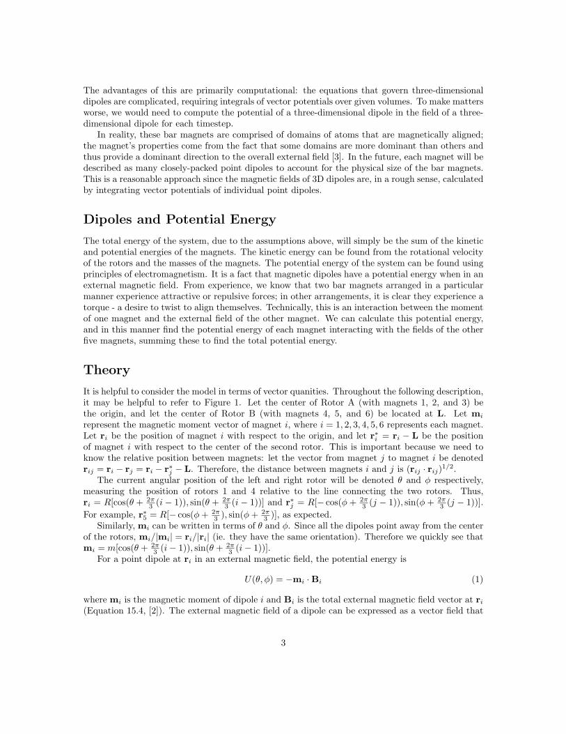
The advantages of this are primarily computational: the equations that govern three-dimensionaldipoles are complicated, requiring integrals of vector potentials over given volumes. To make mattersworse, we would need to compute the potential of a three-dimensional dipole in the field of a three-dimensional dipole for each timestep.

In reality, these bar magnets are comprised of domains of atoms that are magnetically aligned;the magnet’s properties come from the fact that some domains are more dominant than others andthus provide a dominant direction to the overall external field [3]. In the future, each magnet will bedescribed as many closely-packed point dipoles to account for the physical size of the bar magnets.This is a reasonable approach since the magnetic fields of 3D dipoles are, in a rough sense, calculatedby integrating vector potentials of individual point dipoles.

Dipoles and Potential Energy

The total energy of the system, due to the assumptions above, will simply be the sum of the kineticand potential energies of the magnets. The kinetic energy can be found from the rotational velocityof the rotors and the masses of the magnets. The potential energy of the system can be found usingprinciples of electromagnetism. It is a fact that magnetic dipoles have a potential energy when in anexternal magnetic field. From experience, we know that two bar magnets arranged in a particularmanner experience attractive or repulsive forces; in other arrangements, it is clear they experience atorque - a desire to twist to align themselves. Technically, this is an interaction between the momentof one magnet and the external field of the other magnet. We can calculate this potential energy,and in this manner find the potential energy of each magnet interacting with the fields of the otherfive magnets, summing these to find the total potential energy.

Theory

It is helpful to consider the model in terms of vector quanities. Throughout the following description,it may be helpful to refer to Figure 1. Let the center of Rotor A (with magnets 1, 2, and 3) bethe origin, and let the center of Rotor B (with magnets 4, 5, and 6) be located at L. Let mi

represent the magnetic moment vector of magnet i, where i = 1, 2, 3, 4, 5, 6 represents each magnet.Let ri be the position of magnet i with respect to the origin, and let r∗i = ri − L be the positionof magnet i with respect to the center of the second rotor. This is important because we need toknow the relative position between magnets: let the vector from magnet j to magnet i be denotedrij = ri − rj = ri − r∗j − L. Therefore, the distance between magnets i and j is (rij · rij)1/2.

The current angular position of the left and right rotor will be denoted θ and φ respectively,measuring the position of rotors 1 and 4 relative to the line connecting the two rotors. Thus,ri = R[cos(θ + 2π

3 (i − 1)), sin(θ + 2π3 (i − 1))] and r∗j = R[− cos(φ + 2π

3 (j − 1)), sin(φ + 2π3 (j − 1))].

For example, r∗5 = R[− cos(φ + 2π3 ), sin(φ + 2π

3 )], as expected.Similarly, mi can be written in terms of θ and φ. Since all the dipoles point away from the center

of the rotors, mi/|mi| = ri/|ri| (ie. they have the same orientation). Therefore we quickly see thatmi = m[cos(θ + 2π

3 (i − 1)), sin(θ + 2π3 (i − 1))].

For a point dipole at ri in an external magnetic field, the potential energy is

U(θ, φ) = −mi ·Bi (1)

where mi is the magnetic moment of dipole i and Bi is the total external magnetic field vector at ri

(Equation 15.4, [2]). The external magnetic field of a dipole can be expressed as a vector field that

3

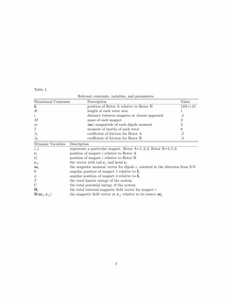
Table 1.

Relevant constants, variables, and parameters.Situational Constants Description ValueL position of Rotor A relative to Rotor B (2R+ε,0)R length of each rotor arm 1ε distance between magnets at closest approach .4M mass of each magnet 2m |m|=magnitude of each dipole moment 3I moment of inertia of each rotor 6β1 coefficient of friction for Rotor A .2β2 coefficient of friction for Rotor B .3

Dynamic Variables Descriptioni, j represents a particular magnet. Rotor A=1, 2, 3, Rotor B=4, 5, 6.ri position of magnet i relative to Rotor Ar∗i position of magnet i relative to Rotor Brij the vector with tail rj and head ri

mi the magnetic moment vector for dipole i, oriented in the direction from S-Nθ angular position of magnet 1 relative to Lφ angular position of magnet 4 relative to LT the total kinetic energy of the systemU the total potential energy of the systemBi the total external magnetic field vector for magnet iB(mj , rij) the magnetic field vector at rij relative to its source mj

4

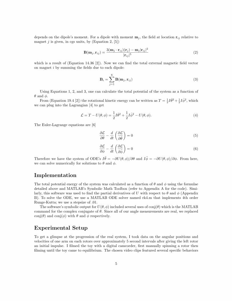
depends on the dipole’s moment. For a dipole with moment mj , the field at location rij relative tomagnet j is given, in cgs units, by (Equation 2, [5])

B(mj , rij) =3(mj · rij)(rj) −mj |rij |2

|rij |5(2)

which is a result of (Equation 14.36 [2]). Now we can find the total external magnetic field vectoron magnet i by summing the fields due to each dipole:

Bi =6∑

j=1

B(mj , rij) (3)

Using Equations 1, 2, and 3, one can calculate the total potential of the system as a function ofθ and φ.

From (Equation 19.4 [2]) the rotational kinetic energy can be written as T = 12Iθ̇2 + 1

2Iφ̇2, whichwe can plug into the Lagrangian [4] to get

L = T − U(θ, φ) =12Iθ̇2 +

12Iφ̇2 − U(θ, φ). (4)

The Euler-Lagrange equations are [6]

∂L∂θ

− d

dt

(∂L∂θ̇

)= 0 (5)

∂L∂φ

− d

dt

(∂L∂φ̇

)= 0 (6)

Therefore we have the system of ODE’s Iθ̈ = −∂U(θ, φ)/∂θ and Iφ̈ = −∂U(θ, φ)/∂φ. From here,we can solve numerically for solutions to θ and φ.

Implementation

The total potential energy of the system was calculated as a function of θ and φ using the formulaedetailed above and MATLAB’s Symbolic Math Toolbox (refer to Appendix A for the code). Simi-larly, this software was used to find the partial derivatives of U with respect to θ and φ (AppendixB). To solve the ODE, we use a MATLAB ODE solver named rk4.m that implements 4th orderRunge-Kutta; we use a stepsize of .01.

The software’s symbolic output for U(θ, φ) included several uses of conj(θ) which is the MATLABcommand for the complex conjugate of θ. Since all of our angle measurements are real, we replacedconj(θ) and conj(φ) with θ and φ respectively.

Experimental Setup

To get a glimpse at the progression of the real system, I took data on the angular positions andvelocities of one arm on each rotors over approximately 5 second intervals after giving the left rotoran initial impulse. I filmed the toy with a digital camcorder, first manually spinning a rotor thenfilming until the toy came to equilibrium. The chosen video clips featured several specific behaviors

5

of the Magnetron that I hope my model will replicate in test simulations (e.g. equilibrium points,“momentum transfer”, etc).

The Magnetron toy was provided by Dr. Ami Radunskaya. The equipment used to take dataincluded a Sony digital camcorder connected via FireWire to an Apple PowerBook laptop withiMovie and VideoPoint software. This setup allowed for a capture rate up to 30 fps. I markedone arm on each rotor with chalk for a visual cue so that using DataPoint would be more precise.Analysis in VideoPoint was performed as accurately as possible with the project’s time constraints.

Discussion

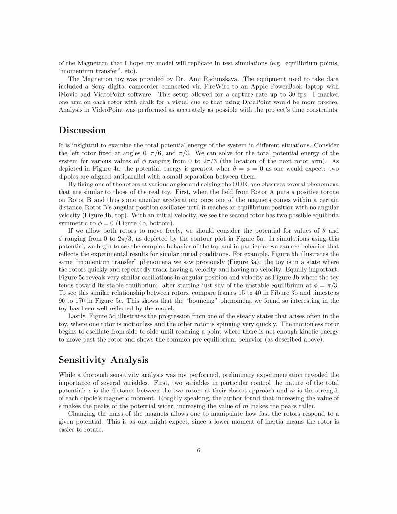
It is insightful to examine the total potential energy of the system in different situations. Considerthe left rotor fixed at angles 0, π/6, and π/3. We can solve for the total potential energy of thesystem for various values of φ ranging from 0 to 2π/3 (the location of the next rotor arm). Asdepicted in Figure 4a, the potential energy is greatest when θ = φ = 0 as one would expect: twodipoles are aligned antiparallel with a small separation between them.

By fixing one of the rotors at various angles and solving the ODE, one observes several phenomenathat are similar to those of the real toy. First, when the field from Rotor A puts a positive torqueon Rotor B and thus some angular acceleration; once one of the magnets comes within a certaindistance, Rotor B’s angular position oscillates until it reaches an equilibrium position with no angularvelocity (Figure 4b, top). With an initial velocity, we see the second rotor has two possible equilibriasymmetric to φ = 0 (Figure 4b, bottom).

If we allow both rotors to move freely, we should consider the potential for values of θ andφ ranging from 0 to 2π/3, as depicted by the contour plot in Figure 5a. In simulations using thispotential, we begin to see the complex behavior of the toy and in particular we can see behavior thatreflects the experimental results for similar initial conditions. For example, Figure 5b illustrates thesame “momentum transfer” phenomena we saw previously (Figure 3a): the toy is in a state wherethe rotors quickly and repeatedly trade having a velocity and having no velocity. Equally important,Figure 5c reveals very similar oscillations in angular position and velocity as Figure 3b where the toytends toward its stable equilibrium, after starting just shy of the unstable equilibrium at φ = π/3.To see this similar relationship between rotors, compare frames 15 to 40 in Fibure 3b and timesteps90 to 170 in Figure 5c. This shows that the “bouncing” phenomena we found so interesting in thetoy has been well reflected by the model.

Lastly, Figure 5d illustrates the progression from one of the steady states that arises often in thetoy, where one rotor is motionless and the other rotor is spinning very quickly. The motionless rotorbegins to oscillate from side to side until reaching a point where there is not enough kinetic energyto move past the rotor and shows the common pre-equilibrium behavior (as described above).

Sensitivity Analysis

While a thorough sensitivity analysis was not performed, preliminary experimentation revealed theimportance of several variables. First, two variables in particular control the nature of the totalpotential: ε is the distance between the two rotors at their closest approach and m is the strengthof each dipole’s magnetic moment. Roughly speaking, the author found that increasing the value ofε makes the peaks of the potential wider; increasing the value of m makes the peaks taller.

Changing the mass of the magnets allows one to manipulate how fast the rotors respond to agiven potential. This is as one might expect, since a lower moment of inertia means the rotor iseasier to rotate.

6

The chosen ODE solver and its respective stepsize appears to have significant effects on theresults, but their exact influence is still unclear. The author does know that with high velocities andtoo large a stepsize, rotors often pass by each other when they would normally “bounce” away inthe opposite direction. Further investigation might provide an optimal combination of realism andcomputational time.

Conclusion

This paper presents a model for the Magnetron toy that uses a Lagrangian formulation by solvingfor the total energy of the system, considering the potential energies of dipoles in the fields of otherdipoles. Preliminary solutions show that the model successfully captures several of the phenomenaof the real toy: “momentum transfers,” “bouncing,” as well as the correct equilibria and steadystates. Some behavior has not been observed in the model, however. The most notable behaviormissing often accompanies the velocity matching behavior, where rotors transition from both havingpositive angular velocity to both having negative angular velocity.

Intuitively, most would consider the toy’s dynamics complex, perhaps even describe it as chaotic.In this vein, future work will determine if there is a dependence on initial conditions and approachthe solutions from a more analytic standpoint in the hopes of affirming our intuition.

7

Bibliography

[1] Jimmy Corno. Chaotic Magnetic Spinner Toy Dynamics (2003).http://chaosbook.org/projects/Corno/Corno.pdf (last accessed 5/3/2005).

[2] Richard P. Feynman. Feynman Lectures on Physics. 1989.

[3] R. Nave. Magnetic Domains and Ferromagnetism. http://hyperphysics.phy-astr.gsu.edu/hbase/hframe.html (last accessed 5/9/2005).

[4] Eric W. Weisstein. ”Lagrangian.” From ScienceWorld –A Wolfram Web Resource.http://scienceworld.wolfram.com/physics/Lagrangian.html (last accessed 5/9/2005).

[5] Eric W. Weisstein. ”Magnetic Dipole.” From ScienceWorld –A Wolfram Web Re-source. http://mathworld.wolfram.com/Euler-LagrangeDifferentialEquation.html (last accessed5/3/2005).

[6] Eric W. Weisstein. ”Euler-Lagrange Differential Equation.” From MathWorld–A WolframWeb Resource. http://scienceworld.wolfram.com/physics/MagneticDipole.html (last accessed5/3/2005).

8

Appendix A

% find_p.m% MATLAB code for Magnetron Project - Chris DuBois% Symbolically find U as a function of theta and phi.

clear;syms theta phi L C R epsilon m m1 m2 m3 m4 m5 m6 r r1 r2 r3 r4 r5 r6;syms U U1 U2 U3 U4 U5 U6;syms B1 B2 B3 B4 B5 B6;syms B14 B15 B16 B24 B25 B26 B34 B35 B36 B41 B42 B43 B51 B52 B53 B61 B62 B63;syms thetadotdot phidotdot I;

% Find mi and ri in vector form.L=2*R+epsilon;m1=m*[cos(theta);sin(theta)];m2=m*[cos(theta+2*pi/3);sin(theta+2*pi/3)];m3=m*[cos(theta+4*pi/3);sin(theta+4*pi/3)];m4=m*[-cos(phi);sin(phi)];m5=m*[-cos(phi+2*pi/3);sin(phi+2*pi/3)];m6=m*[-cos(phi+4*pi/3);sin(phi+4*pi/3)];r1=[cos(theta);sin(theta)];r2=[cos(theta+2*pi/3);sin(theta+2*pi/3)];r3=[cos(theta+4*pi/3);sin(theta+4*pi/3)];r4=[L-cos(phi);sin(phi)];r5=[L-cos(phi+2*pi/3);sin(phi+2*pi/3)];r6=[L-cos(phi+4*pi/3);sin(phi+4*pi/3)];

% Magnetic Field on Rotor 1ri=r1;rj=r4;mi=m1;mj=m4;r=ri-rj;rm=dot(r,r)^.5;B14=(3*r*dot(mj,r)-mj*rm^2)/rm^5;ri=r1;rj=r5;mi=m1;mj=m5;r=ri-rj;rm=dot(r,r)^.5;B15=(3*(ri-rj)*dot(mj,ri-rj)-mj*dot(ri-rj,ri-rj)^2)/dot(ri-rj,ri-rj)^5;B15=C*(3*r*dot(mj,r)-mj*rm^2)/rm^5;

ri=r1;rj=r6;mi=m1;

9

mj=m6;r=ri-rj;rm=dot(r,r)^.5;B16=(3*(ri-rj)*dot(mj,ri-rj)-mj*dot(ri-rj,ri-rj)^2)/dot(ri-rj,ri-rj)^5;B16=C*(3*r*dot(mj,r)-mj*rm^2)/rm^5;

B1=B14+B15+B16;

% Magnetic Field on Rotor 2ri=r2;rj=r4;mi=m2;mj=m4;r=ri-rj;rm=dot(r,r)^.5;B24=(3*(ri-rj)*dot(mj,ri-rj)-mj*dot(ri-rj,ri-rj)^2)/dot(ri-rj,ri-rj)^5;B24=C*(3*r*dot(mj,r)-mj*rm^2)/rm^5;ri=r2;rj=r5;mi=m2;mj=m5;r=ri-rj;rm=dot(r,r)^.5;B25=(3*(ri-rj)*dot(mj,ri-rj)-mj*dot(ri-rj,ri-rj)^2)/dot(ri-rj,ri-rj)^5;B25=C*(3*r*dot(mj,r)-mj*rm^2)/rm^5;ri=r2;rj=r6;mi=m2;mj=m6;r=ri-rj;rm=dot(r,r)^.5;B26=(3*(ri-rj)*dot(mj,ri-rj)-mj*dot(ri-rj,ri-rj)^2)/dot(ri-rj,ri-rj)^5;B26=C*(3*r*dot(mj,r)-mj*rm^2)/rm^5;

B2=B24+B25+B26;

% Magnetic Field on Rotor 3ri=r3;rj=r4;mi=m3;mj=m4;r=ri-rj;rm=dot(r,r)^.5;B34=(3*(ri-rj)*dot(mj,ri-rj)-mj*dot(ri-rj,ri-rj)^2)/dot(ri-rj,ri-rj)^5;B34=C*(3*r*dot(mj,r)-mj*rm^2)/rm^5;ri=r3;rj=r5;mi=m3;

10

mj=m5;r=ri-rj;rm=dot(r,r)^.5;B35=(3*(ri-rj)*dot(mj,ri-rj)-mj*dot(ri-rj,ri-rj)^2)/dot(ri-rj,ri-rj)^5;B35=C*(3*r*dot(mj,r)-mj*rm^2)/rm^5;ri=r3;rj=r6;mi=m3;mj=m6;r=ri-rj;rm=dot(r,r)^.5;B36=(3*(ri-rj)*dot(mj,ri-rj)-mj*dot(ri-rj,ri-rj)^2)/dot(ri-rj,ri-rj)^5;B36=C*(3*r*dot(mj,r)-mj*rm^2)/rm^5;

B3=B34+B35+B36;

% Magnetic Field on Rotor 4ri=r4;rj=r1;mi=m4;mj=m1;r=ri-rj;rm=dot(r,r)^.5;B41=(3*(ri-rj)*dot(mj,ri-rj)-mj*dot(ri-rj,ri-rj)^2)/dot(ri-rj,ri-rj)^5;B41=C*(3*r*dot(mj,r)-mj*rm^2)/rm^5;ri=r4;rj=r2;mi=m4;mj=m2;r=ri-rj;rm=dot(r,r)^.5;B42=(3*(ri-rj)*dot(mj,ri-rj)-mj*dot(ri-rj,ri-rj)^2)/dot(ri-rj,ri-rj)^5;B42=C*(3*r*dot(mj,r)-mj*rm^2)/rm^5;ri=r4;rj=r3;mi=m4;mj=m3;r=ri-rj;rm=dot(r,r)^.5;B43=(3*(ri-rj)*dot(mj,ri-rj)-mj*dot(ri-rj,ri-rj)^2)/dot(ri-rj,ri-rj)^5;B43=C*(3*r*dot(mj,r)-mj*rm^2)/rm^5;

B4=B41+B42+B43;

% Magnetic Field on Rotor 5ri=r5;rj=r1;mi=m5;

11

mj=m1;r=ri-rj;rm=dot(r,r)^.5;B51=(3*(ri-rj)*dot(mj,ri-rj)-mj*dot(ri-rj,ri-rj)^2)/dot(ri-rj,ri-rj)^5;B51=C*(3*r*dot(mj,r)-mj*rm^2)/rm^5;ri=r5;rj=r2;mi=m5;mj=m2;r=ri-rj;rm=dot(r,r)^.5;B52=(3*(ri-rj)*dot(mj,ri-rj)-mj*dot(ri-rj,ri-rj)^2)/dot(ri-rj,ri-rj)^5;B52=C*(3*r*dot(mj,r)-mj*rm^2)/rm^5;ri=r5;rj=r3;mi=m5;mj=m3;r=ri-rj;rm=dot(r,r)^.5;B53=(3*(ri-rj)*dot(mj,ri-rj)-mj*dot(ri-rj,ri-rj)^2)/dot(ri-rj,ri-rj)^5;B53=C*(3*r*dot(mj,r)-mj*rm^2)/rm^5;

B5=B51+B52+B53;

% Magnetic Field on Rotor 6ri=r6;rj=r1;mi=m6;mj=m1;r=ri-rj;rm=dot(r,r)^.5;B61=(3*(ri-rj)*dot(mj,ri-rj)-mj*dot(ri-rj,ri-rj)^2)/dot(ri-rj,ri-rj)^5;B61=C*(3*r*dot(mj,r)-mj*rm^2)/rm^5;ri=r6;rj=r2;mi=m6;mj=m2;r=ri-rj;rm=dot(r,r)^.5;B62=(3*(ri-rj)*dot(mj,ri-rj)-mj*dot(ri-rj,ri-rj)^2)/dot(ri-rj,ri-rj)^5;B62=C*(3*r*dot(mj,r)-mj*rm^2)/rm^5;ri=r6;rj=r3;mi=m6;mj=m3;r=ri-rj;rm=dot(r,r)^.5;B63=(3*(ri-rj)*dot(mj,ri-rj)-mj*dot(ri-rj,ri-rj)^2)/dot(ri-rj,ri-rj)^5;

12

B63=C*(3*r*dot(mj,r)-mj*rm^2)/rm^5;

B6=B61+B62+B63;

% Total Potential EnergiesU1=-dot(m1,B1);U2=-dot(m2,B2);U3=-dot(m3,B3);U4=-dot(m4,B4);U5=-dot(m5,B5);U6=-dot(m6,B6);

Utotal=U1+U2+U3+U4+U5+U6;save Utotal;

Appendix B

% U.m% MATLAB code for Magnetron Project - Chris DuBois% Here, we show MATLAB’s solution for Utotal found by find_p.m% Unew is Utotal without any ’conj’ functions.% We also find dUnew/dtheta and dUnew/dphi symbolically and save them% for use in other code.

Unew=-(m*cos(theta))*(((-(m*cos(phi))*(cos(theta)-2*R-epsilon+cos(phi))+(m*sin(phi))*(sin(theta)-sin(phi)))*(3*cos(theta)-6*R-3*epsilon+3*cos(phi))+((cos(theta)-2*R-epsilon+cos(phi))*(cos(theta)-2*R-epsilon+cos(phi))+(sin(theta)-sin(phi))*(sin(theta)-sin(phi)))*m*cos(phi))/((cos(theta)-2*R-epsilon+cos(phi))*(cos(theta)-2*R-epsilon+cos(phi))+(sin(theta)-sin(phi))*(sin(theta)-sin(phi)))^(5/2)+C*(((m*sin(phi+1/6*pi))*(cos(theta)-2*R-epsilon-sin(phi+1/6*pi))+(m*cos(phi+1/6*pi))*(sin(theta)-cos(phi+1/6*pi)))*(3*cos(theta)-6*R-3*epsilon-3*sin(phi+1/6*pi))-((cos(theta)-2*R-epsilon-sin(phi+1/6*pi))*(cos(theta)-2*R-epsilon-sin(phi+1/6*pi))+(sin(theta)-cos(phi+1/6*pi))*(sin(theta)-cos(phi+1/6*pi)))*m*sin(phi+1/6*pi))/((cos(theta)-2*R-epsilon-sin(phi+1/6*pi))*(cos(theta)-2*R-epsilon-sin(phi+1/6*pi))+(sin(theta)-cos(phi+1/6*pi))*(sin(theta)-cos(phi+1/6*pi)))^(5/2)+C*(((m*cos(phi+1/3*pi))*(cos(theta)-2*R-epsilon-cos(phi+1/3*pi))-(m*sin(phi+1/3*pi))*(sin(theta)+sin(phi+1/3*pi)))*(3*cos(theta)-6*R-3*epsilon-3*cos(phi+1/3*pi))-((cos(theta)-2*R-epsilon-cos(phi+1/3*pi))*(cos(theta)-2*R-epsilon-cos(phi+1/3*pi))+(sin(theta)+sin(phi+1/3*pi))*(sin(theta)+sin(phi+1/3*pi)))*m*cos(phi+1/3*pi))/((cos(theta)-2*R-epsilon-cos(phi+1/3*pi))*(cos(theta)-2*R-epsilon-cos(phi+1/3*pi))+(sin(theta)+sin(phi+1/3*pi))*(sin(theta)+sin(phi+1/3*pi)))^(5/2))-(m*sin(theta))*(((-(m*cos(phi))*(cos(theta)-2*R-epsilon+cos(phi))+(m*sin(phi))*(sin(theta)-sin(phi)))*(3*sin(theta)-3*sin(phi))-((cos(theta)-2*R-epsilon+cos(phi))*(cos(theta)-2*R-epsilon+cos(phi))+(sin(theta)-sin(phi))*(sin(theta)-sin(phi)))*m*sin(phi))/((cos(theta)-2*R-epsilon+cos(phi))*(cos(theta)-2*R-epsilon+

13

cos(phi))+(sin(theta)-sin(phi))*(sin(theta)-sin(phi)))^(5/2)+C*(((m*sin(phi+1/6*pi))*(cos(theta)-2*R-epsilon-sin(phi+1/6*pi))+(m*cos(phi+1/6*pi))*(sin(theta)-cos(phi+1/6*pi)))*(3*sin(theta)-3*cos(phi+1/6*pi))-((cos(theta)-2*R-epsilon-sin(phi+1/6*pi))*(cos(theta)-2*R-epsilon-sin(phi+1/6*pi))+(sin(theta)-cos(phi+1/6*pi))*(sin(theta)-cos(phi+1/6*pi)))*m*cos(phi+1/6*pi))/((cos(theta)-2*R-epsilon-sin(phi+1/6*pi))*(cos(theta)-2*R-epsilon-sin(phi+1/6*pi))+(sin(theta)-cos(phi+1/6*pi))*(sin(theta)-cos(phi+1/6*pi)))^(5/2)+C*(((m*cos(phi+1/3*pi))*(cos(theta)-2*R-epsilon-cos(phi+1/3*pi))-(m*sin(phi+1/3*pi))*(sin(theta)+sin(phi+1/3*pi)))*(3*sin(theta)+3*sin(phi+1/3*pi))+((cos(theta)-2*R-epsilon-cos(phi+1/3*pi))*(cos(theta)-2*R-epsilon-cos(phi+1/3*pi))+(sin(theta)+sin(phi+1/3*pi))*(sin(theta)+sin(phi+1/3*pi)))*m*sin(phi+1/3*pi))/((cos(theta)-2*R-epsilon-cos(phi+1/3*pi))*(cos(theta)-2*R-epsilon-cos(phi+1/3*pi))+(sin(theta)+sin(phi+1/3*pi))*(sin(theta)+sin(phi+1/3*pi)))^(5/2))+(m*sin(theta+1/6*pi))*(C*((-(m*cos(phi))*(-sin(theta+1/6*pi)-2*R-epsilon+cos(phi))+(m*sin(phi))*(cos(theta+1/6*pi)-sin(phi)))*(-3*sin(theta+1/6*pi)-6*R-3*epsilon+3*cos(phi))+((-sin(theta+1/6*pi)-2*R-epsilon+cos(phi))*(-sin(theta+1/6*pi)-2*R-epsilon+cos(phi))+(cos(theta+1/6*pi)-sin(phi))*(cos(theta+1/6*pi)-sin(phi)))*m*cos(phi))/((-sin(theta+1/6*pi)-2*R-epsilon+cos(phi))*(-sin(theta+1/6*pi)-2*R-epsilon+cos(phi))+(cos(theta+1/6*pi)-sin(phi))*(cos(theta+1/6*pi)-sin(phi)))^(5/2)+C*(((m*sin(phi+1/6*pi))*(-sin(theta+1/6*pi)-2*R-epsilon-sin(phi+1/6*pi))+(m*cos(phi+1/6*pi))*(cos(theta+1/6*pi)-cos(phi+1/6*pi)))*(-3*sin(theta+1/6*pi)-6*R-3*epsilon-3*sin(phi+1/6*pi))-((-sin(theta+1/6*pi)-2*R-epsilon-sin(phi+1/6*pi))*(-sin(theta+1/6*pi)-2*R-epsilon-sin(phi+1/6*pi))+(cos(theta+1/6*pi)-cos(phi+1/6*pi))*(cos(theta+1/6*pi)-cos(phi+1/6*pi)))*m*sin(phi+1/6*pi))/((-sin(theta+1/6*pi)-2*R-epsilon-sin(phi+1/6*pi))*(-sin(theta+1/6*pi)-2*R-epsilon-sin(phi+1/6*pi))+(cos(theta+1/6*pi)-cos(phi+1/6*pi))*(cos(theta+1/6*pi)-cos(phi+1/6*pi)))^(5/2)+C*(((m*cos(phi+1/3*pi))*(-sin(theta+1/6*pi)-2*R-epsilon-cos(phi+1/3*pi))-(m*sin(phi+1/3*pi))*(cos(theta+1/6*pi)+sin(phi+1/3*pi)))*(-3*sin(theta+1/6*pi)-6*R-3*epsilon-3*cos(phi+1/3*pi))-((-sin(theta+1/6*pi)-2*R-epsilon-cos(phi+1/3*pi))*(-sin(theta+1/6*pi)-2*R-epsilon-cos(phi+1/3*pi))+(cos(theta+1/6*pi)+sin(phi+1/3*pi))*(cos(theta+1/6*pi)+sin(phi+1/3*pi)))*m*cos(phi+1/3*pi))/((-sin(theta+1/6*pi)-2*R-epsilon-cos(phi+1/3*pi))*(-sin(theta+1/6*pi)-2*R-epsilon-cos(phi+1/3*pi))+(cos(theta+1/6*pi)+sin(phi+1/3*pi))*(cos(theta+1/6*pi)+sin(phi+1/3*pi)))^(5/2))-(m*cos(theta+1/6*pi))*(C*((-(m*cos(phi))*(-sin(theta+1/6*pi)-2*R-epsilon+cos(phi))+(m*sin(phi))*(cos(theta+1/6*pi)-sin(phi)))*(3*cos(theta+1/6*pi)-3*sin(phi))-((-sin(theta+1/6*pi)-2*R-epsilon+cos(phi))*(-sin(theta+1/6*pi)-2*R-epsilon+cos(phi))+(cos(theta+1/6*pi)-sin(phi))*(cos(theta+1/6*pi)-sin(phi)))*m*sin(phi))/((-sin(theta+1/6*pi)-2*R-epsilon+cos(phi))*(-sin(theta+1/6*pi)-2*R-epsilon+cos(phi))+(cos(theta+1/6*pi)-sin(phi))*(cos(theta+1/6*pi)-sin(phi)))^(5/2)+C*(((m*sin(phi+1/6*pi))*(-sin(theta+1/6*pi)-2*R-epsilon-sin(phi+1/6*pi))+(m*cos(phi+1/6*pi))*(cos(theta+1/6*pi)-cos(phi+1/6*pi)))*(3*cos(theta+1/6*pi)-3*cos(phi+1/6*pi))-((-sin(theta+1/6*pi)-2*R-epsilon-sin(phi+1/6*pi))*(-sin(theta+1/6*pi)-2*R-epsilon-sin(phi+1/6*pi))+(cos(theta+1/6*pi)-cos(phi+1/6*pi))*(cos(theta+1/6*pi)-cos(phi+1/6*pi)))*m*cos(phi+1/6*pi))/((-sin(theta+1/6*pi)-2*R-epsilon-sin(phi+1/6*pi))*(-sin(theta+1/6*pi)-2*R-epsilon-sin(phi+1/6*pi))+(cos(theta+1/6*pi)-

14

cos(phi+1/6*pi))*(cos(theta+1/6*pi)-cos(phi+1/6*pi)))^(5/2)+C*(((m*cos(phi+1/3*pi))*(-sin(theta+1/6*pi)-2*R-epsilon-cos(phi+1/3*pi))-(m*sin(phi+1/3*pi))*(cos(theta+1/6*pi)+sin(phi+1/3*pi)))*(3*cos(theta+1/6*pi)+3*sin(phi+1/3*pi))+((-sin(theta+1/6*pi)-2*R-epsilon-cos(phi+1/3*pi))*(-sin(theta+1/6*pi)-2*R-epsilon-cos(phi+1/3*pi))+(cos(theta+1/6*pi)+sin(phi+1/3*pi))*(cos(theta+1/6*pi)+sin(phi+1/3*pi)))*m*sin(phi+1/3*pi))/((-sin(theta+1/6*pi)-2*R-epsilon-cos(phi+1/3*pi))*(-sin(theta+1/6*pi)-2*R-epsilon-cos(phi+1/3*pi))+(cos(theta+1/6*pi)+sin(phi+1/3*pi))*(cos(theta+1/6*pi)+sin(phi+1/3*pi)))^(5/2))+(m*cos(theta+1/3*pi))*(C*((-(m*cos(phi))*(-cos(theta+1/3*pi)-2*R-epsilon+cos(phi))+(m*sin(phi))*(-sin(theta+1/3*pi)-sin(phi)))*(-3*cos(theta+1/3*pi)-6*R-3*epsilon+3*cos(phi))+((-cos(theta+1/3*pi)-2*R-epsilon+cos(phi))*(-cos(theta+1/3*pi)-2*R-epsilon+cos(phi))+(-sin(theta+1/3*pi)-sin(phi))*(-sin(theta+1/3*pi)-sin(phi)))*m*cos(phi))/((-cos(theta+1/3*pi)-2*R-epsilon+cos(phi))*(-cos(theta+1/3*pi)-2*R-epsilon+cos(phi))+(-sin(theta+1/3*pi)-sin(phi))*(-sin(theta+1/3*pi)-sin(phi)))^(5/2)+C*(((m*sin(phi+1/6*pi))*(-cos(theta+1/3*pi)-2*R-epsilon-sin(phi+1/6*pi))+(m*cos(phi+1/6*pi))*(-sin(theta+1/3*pi)-cos(phi+1/6*pi)))*(-3*cos(theta+1/3*pi)-6*R-3*epsilon-3*sin(phi+1/6*pi))-((-cos(theta+1/3*pi)-2*R-epsilon-sin(phi+1/6*pi))*(-cos(theta+1/3*pi)-2*R-epsilon-sin(phi+1/6*pi))+(-sin(theta+1/3*pi)-cos(phi+1/6*pi))*(-sin(theta+1/3*pi)-cos(phi+1/6*pi)))*m*sin(phi+1/6*pi))/((-cos(theta+1/3*pi)-2*R-epsilon-sin(phi+1/6*pi))*(-cos(theta+1/3*pi)-2*R-epsilon-sin(phi+1/6*pi))+(-sin(theta+1/3*pi)-cos(phi+1/6*pi))*(-sin(theta+1/3*pi)-cos(phi+1/6*pi)))^(5/2)+C*(((m*cos(phi+1/3*pi))*(-cos(theta+1/3*pi)-2*R-epsilon-cos(phi+1/3*pi))-(m*sin(phi+1/3*pi))*(-sin(theta+1/3*pi)+sin(phi+1/3*pi)))*(-3*cos(theta+1/3*pi)-6*R-3*epsilon-3*cos(phi+1/3*pi))-((-cos(theta+1/3*pi)-2*R-epsilon-cos(phi+1/3*pi))*(-cos(theta+1/3*pi)-2*R-epsilon-cos(phi+1/3*pi))+(-sin(theta+1/3*pi)+sin(phi+1/3*pi))*(-sin(theta+1/3*pi)+sin(phi+1/3*pi)))*m*cos(phi+1/3*pi))/((-cos(theta+1/3*pi)-2*R-epsilon-cos(phi+1/3*pi))*(-cos(theta+1/3*pi)-2*R-epsilon-cos(phi+1/3*pi))+(-sin(theta+1/3*pi)+sin(phi+1/3*pi))*(-sin(theta+1/3*pi)+sin(phi+1/3*pi)))^(5/2))+(m*sin(theta+1/3*pi))*(C*((-(m*cos(phi))*(-cos(theta+1/3*pi)-2*R-epsilon+cos(phi))+(m*sin(phi))*(-sin(theta+1/3*pi)-sin(phi)))*(-3*sin(theta+1/3*pi)-3*sin(phi))-((-cos(theta+1/3*pi)-2*R-epsilon+cos(phi))*(-cos(theta+1/3*pi)-2*R-epsilon+cos(phi))+(-sin(theta+1/3*pi)-sin(phi))*(-sin(theta+1/3*pi)-sin(phi)))*m*sin(phi))/((-cos(theta+1/3*pi)-2*R-epsilon+cos(phi))*(-cos(theta+1/3*pi)-2*R-epsilon+cos(phi))+(-sin(theta+1/3*pi)-sin(phi))*(-sin(theta+1/3*pi)-sin(phi)))^(5/2)+C*(((m*sin(phi+1/6*pi))*(-cos(theta+1/3*pi)-2*R-epsilon-sin(phi+1/6*pi))+(m*cos(phi+1/6*pi))*(-sin(theta+1/3*pi)-cos(phi+1/6*pi)))*(-3*sin(theta+1/3*pi)-3*cos(phi+1/6*pi))-((-cos(theta+1/3*pi)-2*R-epsilon-sin(phi+1/6*pi))*(-cos(theta+1/3*pi)-2*R-epsilon-sin(phi+1/6*pi))+(-sin(theta+1/3*pi)-cos(phi+1/6*pi))*(-sin(theta+1/3*pi)-cos(phi+1/6*pi)))*m*cos(phi+1/6*pi))/((-cos(theta+1/3*pi)-2*R-epsilon-sin(phi+1/6*pi))*(-cos(theta+1/3*pi)-2*R-epsilon-sin(phi+1/6*pi))+(-sin(theta+1/3*pi)-cos(phi+1/6*pi))*(-sin(theta+1/3*pi)-cos(phi+1/6*pi)))^(5/2)+C*(((m*cos(phi+1/3*pi))*(-cos(theta+1/3*pi)-2*R-epsilon-cos(phi+1/3*pi))-(m*sin(phi+1/3*pi))*(-sin(theta+1/3*pi)+sin(phi+1/3*pi)))*(-3*sin(theta+1/3*pi)+3*sin(phi+1/3*pi))+((-cos(theta+1/3*pi)-2*R-epsilon-cos(phi+1/3*pi))*(-cos(theta+1/3*pi)-2*R-epsilon-

15

cos(phi+1/3*pi))+(-sin(theta+1/3*pi)+sin(phi+1/3*pi))*(-sin(theta+1/3*pi)+sin(phi+1/3*pi)))*m*sin(phi+1/3*pi))/((-cos(theta+1/3*pi)-2*R-epsilon-cos(phi+1/3*pi))*(-cos(theta+1/3*pi)-2*R-epsilon-cos(phi+1/3*pi))+(-sin(theta+1/3*pi)+sin(phi+1/3*pi))*(-sin(theta+1/3*pi)+sin(phi+1/3*pi)))^(5/2))+(m*cos(phi))*(C*(((m*cos(theta))*(2*R+epsilon-cos(phi)-cos(theta))+(m*sin(theta))*(sin(phi)-sin(theta)))*(6*R+3*epsilon-3*cos(phi)-3*cos(theta))-((2*R+epsilon-cos(phi)-cos(theta))*(2*R+epsilon-cos(phi)-cos(theta))+(sin(phi)-sin(theta))*(sin(phi)-sin(theta)))*m*cos(theta))/((2*R+epsilon-cos(phi)-cos(theta))*(2*R+epsilon-cos(phi)-cos(theta))+(sin(phi)-sin(theta))*(sin(phi)-sin(theta)))^(5/2)+C*((-(m*sin(theta+1/6*pi))*(2*R+epsilon-cos(phi)+sin(theta+1/6*pi))+(m*cos(theta+1/6*pi))*(sin(phi)-cos(theta+1/6*pi)))*(6*R+3*epsilon-3*cos(phi)+3*sin(theta+1/6*pi))+((2*R+epsilon-cos(phi)+sin(theta+1/6*pi))*(2*R+epsilon-cos(phi)+sin(theta+1/6*pi))+(sin(phi)-cos(theta+1/6*pi))*(sin(phi)-cos(theta+1/6*pi)))*m*sin(theta+1/6*pi))/((2*R+epsilon-cos(phi)+sin(theta+1/6*pi))*(2*R+epsilon-cos(phi)+sin(theta+1/6*pi))+(sin(phi)-cos(theta+1/6*pi))*(sin(phi)-cos(theta+1/6*pi)))^(5/2)+C*((-(m*cos(theta+1/3*pi))*(2*R+epsilon-cos(phi)+cos(theta+1/3*pi))-(m*sin(theta+1/3*pi))*(sin(phi)+sin(theta+1/3*pi)))*(6*R+3*epsilon-3*cos(phi)+3*cos(theta+1/3*pi))+((2*R+epsilon-cos(phi)+cos(theta+1/3*pi))*(2*R+epsilon-cos(phi)+cos(theta+1/3*pi))+(sin(phi)+sin(theta+1/3*pi))*(sin(phi)+sin(theta+1/3*pi)))*m*cos(theta+1/3*pi))/((2*R+epsilon-cos(phi)+cos(theta+1/3*pi))*(2*R+epsilon-cos(phi)+cos(theta+1/3*pi))+(sin(phi)+sin(theta+1/3*pi))*(sin(phi)+sin(theta+1/3*pi)))^(5/2))-(m*sin(phi))*(C*(((m*cos(theta))*(2*R+epsilon-cos(phi)-cos(theta))+(m*sin(theta))*(sin(phi)-sin(theta)))*(3*sin(phi)-3*sin(theta))-((2*R+epsilon-cos(phi)-cos(theta))*(2*R+epsilon-cos(phi)-cos(theta))+(sin(phi)-sin(theta))*(sin(phi)-sin(theta)))*m*sin(theta))/((2*R+epsilon-cos(phi)-cos(theta))*(2*R+epsilon-cos(phi)-cos(theta))+(sin(phi)-sin(theta))*(sin(phi)-sin(theta)))^(5/2)+C*((-(m*sin(theta+1/6*pi))*(2*R+epsilon-cos(phi)+sin(theta+1/6*pi))+(m*cos(theta+1/6*pi))*(sin(phi)-cos(theta+1/6*pi)))*(3*sin(phi)-3*cos(theta+1/6*pi))-((2*R+epsilon-cos(phi)+sin(theta+1/6*pi))*(2*R+epsilon-cos(phi)+sin(theta+1/6*pi))+(sin(phi)-cos(theta+1/6*pi))*(sin(phi)-cos(theta+1/6*pi)))*m*cos(theta+1/6*pi))/((2*R+epsilon-cos(phi)+sin(theta+1/6*pi))*(2*R+epsilon-cos(phi)+sin(theta+1/6*pi))+(sin(phi)-cos(theta+1/6*pi))*(sin(phi)-cos(theta+1/6*pi)))^(5/2)+C*((-(m*cos(theta+1/3*pi))*(2*R+epsilon-cos(phi)+cos(theta+1/3*pi))-(m*sin(theta+1/3*pi))*(sin(phi)+sin(theta+1/3*pi)))*(3*sin(phi)+3*sin(theta+1/3*pi))+((2*R+epsilon-cos(phi)+cos(theta+1/3*pi))*(2*R+epsilon-cos(phi)+cos(theta+1/3*pi))+(sin(phi)+sin(theta+1/3*pi))*(sin(phi)+sin(theta+1/3*pi)))*m*sin(theta+1/3*pi))/((2*R+epsilon-cos(phi)+cos(theta+1/3*pi))*(2*R+epsilon-cos(phi)+cos(theta+1/3*pi))+(sin(phi)+sin(theta+1/3*pi))*(sin(phi)+sin(theta+1/3*pi)))^(5/2))-(m*sin(phi+1/6*pi))*(C*(((m*cos(theta))*(2*R+epsilon+sin(phi+1/6*pi)-cos(theta))+(m*sin(theta))*(cos(phi+1/6*pi)-sin(theta)))*(6*R+3*epsilon+3*sin(phi+1/6*pi)-3*cos(theta))-((2*R+epsilon+sin(phi+1/6*pi)-cos(theta))*(2*R+epsilon+sin(phi+1/6*pi)-cos(theta))+(cos(phi+1/6*pi)-sin(theta))*(cos(phi+1/6*pi)-sin(theta)))*m*cos(theta))/((2*R+epsilon+sin(phi+1/6*pi)-cos(theta))*(2*R+epsilon+sin(phi+1/6*pi)-cos(theta))+(cos(phi+1/6*pi)-sin(theta))*(cos(phi+1/6*pi)-sin(theta)))^(5/2)+C*((-(m*sin(theta+1/6*pi))*(2*R+epsilon+sin(phi+1/6*pi)+sin(theta+1/6*pi))+(m*cos(theta+1/6*pi))*(cos(phi+1/6*pi)-cos(theta+1/6*pi)))*(6*R+3*epsilon+3*sin(phi+1/6*pi)+3*sin(theta+1/6*

16

pi))+((2*R+epsilon+sin(phi+1/6*pi)+sin(theta+1/6*pi))*(2*R+epsilon+sin(phi+1/6*pi)+sin(theta+1/6*pi))+(cos(phi+1/6*pi)-cos(theta+1/6*pi))*(cos(phi+1/6*pi)-cos(theta+1/6*pi)))*m*sin(theta+1/6*pi))/((2*R+epsilon+sin(phi+1/6*pi)+sin(theta+1/6*pi))*(2*R+epsilon+sin(phi+1/6*pi)+sin(theta+1/6*pi))+(cos(phi+1/6*pi)-cos(theta+1/6*pi))*(cos(phi+1/6*pi)-cos(theta+1/6*pi)))^(5/2)+C*((-(m*cos(theta+1/3*pi))*(2*R+epsilon+sin(phi+1/6*pi)+cos(theta+1/3*pi))-(m*sin(theta+1/3*pi))*(cos(phi+1/6*pi)+sin(theta+1/3*pi)))*(6*R+3*epsilon+3*sin(phi+1/6*pi)+3*cos(theta+1/3*pi))+((2*R+epsilon+sin(phi+1/6*pi)+cos(theta+1/3*pi))*(2*R+epsilon+sin(phi+1/6*pi)+cos(theta+1/3*pi))+(cos(phi+1/6*pi)+sin(theta+1/3*pi))*(cos(phi+1/6*pi)+sin(theta+1/3*pi)))*m*cos(theta+1/3*pi))/((2*R+epsilon+sin(phi+1/6*pi)+cos(theta+1/3*pi))*(2*R+epsilon+sin(phi+1/6*pi)+cos(theta+1/3*pi))+(cos(phi+1/6*pi)+sin(theta+1/3*pi))*(cos(phi+1/6*pi)+sin(theta+1/3*pi)))^(5/2))-(m*cos(phi+1/6*pi))*(C*(((m*cos(theta))*(2*R+epsilon+sin(phi+1/6*pi)-cos(theta))+(m*sin(theta))*(cos(phi+1/6*pi)-sin(theta)))*(3*cos(phi+1/6*pi)-3*sin(theta))-((2*R+epsilon+sin(phi+1/6*pi)-cos(theta))*(2*R+epsilon+sin(phi+1/6*pi)-cos(theta))+(cos(phi+1/6*pi)-sin(theta))*(cos(phi+1/6*pi)-sin(theta)))*m*sin(theta))/((2*R+epsilon+sin(phi+1/6*pi)-cos(theta))*(2*R+epsilon+sin(phi+1/6*pi)-cos(theta))+(cos(phi+1/6*pi)-sin(theta))*(cos(phi+1/6*pi)-sin(theta)))^(5/2)+C*((-(m*sin(theta+1/6*pi))*(2*R+epsilon+sin(phi+1/6*pi)+sin(theta+1/6*pi))+(m*cos(theta+1/6*pi))*(cos(phi+1/6*pi)-cos(theta+1/6*pi)))*(3*cos(phi+1/6*pi)-3*cos(theta+1/6*pi))-((2*R+epsilon+sin(phi+1/6*pi)+sin(theta+1/6*pi))*(2*R+epsilon+sin(phi+1/6*pi)+sin(theta+1/6*pi))+(cos(phi+1/6*pi)-cos(theta+1/6*pi))*(cos(phi+1/6*pi)-cos(theta+1/6*pi)))*m*cos(theta+1/6*pi))/((2*R+epsilon+sin(phi+1/6*pi)+sin(theta+1/6*pi))*(2*R+epsilon+sin(phi+1/6*pi)+sin(theta+1/6*pi))+(cos(phi+1/6*pi)-cos(theta+1/6*pi))*(cos(phi+1/6*pi)-cos(theta+1/6*pi)))^(5/2)+C*((-(m*cos(theta+1/3*pi))*(2*R+epsilon+sin(phi+1/6*pi)+cos(theta+1/3*pi))-(m*sin(theta+1/3*pi))*(cos(phi+1/6*pi)+sin(theta+1/3*pi)))*(3*cos(phi+1/6*pi)+3*sin(theta+1/3*pi))+((2*R+epsilon+sin(phi+1/6*pi)+cos(theta+1/3*pi))*(2*R+epsilon+sin(phi+1/6*pi)+cos(theta+1/3*pi))+(cos(phi+1/6*pi)+sin(theta+1/3*pi))*(cos(phi+1/6*pi)+sin(theta+1/3*pi)))*m*sin(theta+1/3*pi))/((2*R+epsilon+sin(phi+1/6*pi)+cos(theta+1/3*pi))*(2*R+epsilon+sin(phi+1/6*pi)+cos(theta+1/3*pi))+(cos(phi+1/6*pi)+sin(theta+1/3*pi))*(cos(phi+1/6*pi)+sin(theta+1/3*pi)))^(5/2))-(m*cos(phi+1/3*pi))*(C*(((m*cos(theta))*(2*R+epsilon+cos(phi+1/3*pi)-cos(theta))+(m*sin(theta))*(-sin(phi+1/3*pi)-sin(theta)))*(6*R+3*epsilon+3*cos(phi+1/3*pi)-3*cos(theta))-((2*R+epsilon+cos(phi+1/3*pi)-cos(theta))*(2*R+epsilon+cos(phi+1/3*pi)-cos(theta))+(-sin(phi+1/3*pi)-sin(theta))*(-sin(phi+1/3*pi)-sin(theta)))*m*cos(theta))/((2*R+epsilon+cos(phi+1/3*pi)-cos(theta))*(2*R+epsilon+cos(phi+1/3*pi)-cos(theta))+(-sin(phi+1/3*pi)-sin(theta))*(-sin(phi+1/3*pi)-sin(theta)))^(5/2)+C*((-(m*sin(theta+1/6*pi))*(2*R+epsilon+cos(phi+1/3*pi)+sin(theta+1/6*pi))+(m*cos(theta+1/6*pi))*(-sin(phi+1/3*pi)-cos(theta+1/6*pi)))*(6*R+3*epsilon+3*cos(phi+1/3*pi)+3*sin(theta+1/6*pi))+((2*R+epsilon+cos(phi+1/3*pi)+sin(theta+1/6*pi))*(2*R+epsilon+cos(phi+1/3*pi)+sin(theta+1/6*pi))+(-sin(phi+1/3*pi)-cos(theta+1/6*pi))*(-sin(phi+1/3*pi)-cos(theta+1/6*pi)))*m*sin(theta+1/6*pi))/((2*R+epsilon+cos(phi+1/3*pi)+sin(theta+1/6*pi))*(2*R+epsilon+cos(phi+1/3*pi)+sin(theta+1/6*pi))+(-sin(phi+1/3*pi)-cos(theta+1/6*pi))*(-sin(phi+1/3*pi)-cos(theta+1/6*pi)))^(5/2)+C*((-(m*cos(theta+1/3*pi))*(2*R+epsilon+cos(phi+1/3*pi)+cos(theta+1/3*pi))-(m*

17

sin(theta+1/3*pi))*(-sin(phi+1/3*pi)+sin(theta+1/3*pi)))*(6*R+3*epsilon+3*cos(phi+1/3*pi)+3*cos(theta+1/3*pi))+((2*R+epsilon+cos(phi+1/3*pi)+cos(theta+1/3*pi))*(2*R+epsilon+cos(phi+1/3*pi)+cos(theta+1/3*pi))+(-sin(phi+1/3*pi)+sin(theta+1/3*pi))*(-sin(phi+1/3*pi)+sin(theta+1/3*pi)))*m*cos(theta+1/3*pi))/((2*R+epsilon+cos(phi+1/3*pi)+cos(theta+1/3*pi))*(2*R+epsilon+cos(phi+1/3*pi)+cos(theta+1/3*pi))+(-sin(phi+1/3*pi)+sin(theta+1/3*pi))*(-sin(phi+1/3*pi)+sin(theta+1/3*pi)))^(5/2))+(m*sin(phi+1/3*pi))*(C*(((m*cos(theta))*(2*R+epsilon+cos(phi+1/3*pi)-cos(theta))+(m*sin(theta))*(-sin(phi+1/3*pi)-sin(theta)))*(-3*sin(phi+1/3*pi)-3*sin(theta))-((2*R+epsilon+cos(phi+1/3*pi)-cos(theta))*(2*R+epsilon+cos(phi+1/3*pi)-cos(theta))+(-sin(phi+1/3*pi)-sin(theta))*(-sin(phi+1/3*pi)-sin(theta)))*m*sin(theta))/((2*R+epsilon+cos(phi+1/3*pi)-cos(theta))*(2*R+epsilon+cos(phi+1/3*pi)-cos(theta))+(-sin(phi+1/3*pi)-sin(theta))*(-sin(phi+1/3*pi)-sin(theta)))^(5/2)+C*((-(m*sin(theta+1/6*pi))*(2*R+epsilon+cos(phi+1/3*pi)+sin(theta+1/6*pi))+(m*cos(theta+1/6*pi))*(-sin(phi+1/3*pi)-cos(theta+1/6*pi)))*(-3*sin(phi+1/3*pi)-3*cos(theta+1/6*pi))-((2*R+epsilon+cos(phi+1/3*pi)+sin(theta+1/6*pi))*(2*R+epsilon+cos(phi+1/3*pi)+sin(theta+1/6*pi))+(-sin(phi+1/3*pi)-cos(theta+1/6*pi))*(-sin(phi+1/3*pi)-cos(theta+1/6*pi)))*m*cos(theta+1/6*pi))/((2*R+epsilon+cos(phi+1/3*pi)+sin(theta+1/6*pi))*(2*R+epsilon+cos(phi+1/3*pi)+sin(theta+1/6*pi))+(-sin(phi+1/3*pi)-cos(theta+1/6*pi))*(-sin(phi+1/3*pi)-cos(theta+1/6*pi)))^(5/2)+C*((-(m*cos(theta+1/3*pi))*(2*R+epsilon+cos(phi+1/3*pi)+cos(theta+1/3*pi))-(m*sin(theta+1/3*pi))*(-sin(phi+1/3*pi)+sin(theta+1/3*pi)))*(-3*sin(phi+1/3*pi)+3*sin(theta+1/3*pi))+((2*R+epsilon+cos(phi+1/3*pi)+cos(theta+1/3*pi))*(2*R+epsilon+cos(phi+1/3*pi)+cos(theta+1/3*pi))+(-sin(phi+1/3*pi)+sin(theta+1/3*pi))*(-sin(phi+1/3*pi)+sin(theta+1/3*pi)))*m*sin(theta+1/3*pi))/((2*R+epsilon+cos(phi+1/3*pi)+cos(theta+1/3*pi))*(2*R+epsilon+cos(phi+1/3*pi)+cos(theta+1/3*pi))+(-sin(phi+1/3*pi)+sin(theta+1/3*pi))*(-sin(phi+1/3*pi)+sin(theta+1/3*pi)))^(5/2))

dUdTheta=diff(Unew,’theta’);dUdPhi=diff(Unew,’phi’);save Unew;save dUdTheta;save dUdPhi;

Appendix C

% graph_p.m% MATLAB code for Magnetron Project - Chris DuBois% Script for plotting potentials

load Utotal;

%%% CONSTANTSR=1;epsilon=.4;M=2;

18

m=3;I=3*M*R^2;beta1=.2;beta2=.3;C=1; % C=\mu_0/4pi

% Step sized=2*pi/3/500;

% Potential Energy Plot for% theta=(0,2pi/3), phi=(0,2pi/3)P=0;i=1;for theta=0:d:2*pi/3

j=1;for phi=0:d:2*pi/3

P(i,j)=eval(U);j=j+1;

endi=i+1;

end

% Potential Energy Plot for% Theta Fixed, Phi (0,2pi/3)

theta=0;i=1;for theta=0:pi/6:pi/3

j=1;for phi=0:d:2*pi/3

P(i,j)=eval(Utotal);j=j+1;

endi=i+1;

endhold off;plot(P(1,:)); hold on;plot(P(2,:));plot(P(3,:));

Appendix D

% main.m% MATLAB code for Magnetron Project - Chris DuBois% Solve the ODEs using rk4

global dUdTheta dUdPhi;

19

load dUdTheta;load dUdPhi;

hold off; clf;[t, y] = rk4(’projectFun’, [0 20], [-pi/6;0;pi/3;30],.005);save run036 y;

Appendix E

% projectFun.m% MATLAB code for Magnetron Project - Chris DuBois% Provides the ODEs to solve

function Yprime = projectFun(t,y)

%%% CONSTANTSR=1;epsilon=.4;M=2;m=3;I=3*M*R^2;beta1=.2;beta2=.3;C=1; % C=\mu_0/4pi

Theta = y(1);ThetaDot = y(2);Phi = y(3);PhiDot = y(4);

theta=mod(Theta,2*pi);phi=mod(Phi,2*pi);

global dUdTheta dUdPhi;

dUdT=eval(dUdTheta);dUdP=eval(dUdPhi);

ThetaDotDot=-dUdT/I;PhiDotDot=-dUdP/I;

Yprime=[ThetaDot;ThetaDotDot-beta1*ThetaDot;PhiDot;PhiDotDot-beta2*PhiDot];

% % Uncomment for fixed theta

20

% Yprime=[Theta;% ThetaDot;% PhiDot;% PhiDotDot-beta2*PhiDot];

21