ICARUS 99, 1--14 (1992)

Modeling the Martian Seasonal C02 Cycle

1. Fitting the Viking Lander Pressure Curves

STEPHEN E . WOOD AND DAVID A. PAIGE

Department of Earth and Space Sciences, University of California, Los Angeles, Los Angeles, California 90024

Received January 29, 1992; revised May 19, 1992

A diurnal and seasonal thermal model is used to simulate the seasonal exchange of carbon dioxide between the atmosphere and polar caps of Mars. Surface CO2 frost condensation and sublima- tion rates are determined by the net effects of radiation, latent heat, and heat conduction in subsurface soil layers. We show that this model can successfully reproduce the measured seasonal pressure variations at the Viking lander 1 site using constant values for frost albedo and emissivity in each hemisphere. An exact treatment of heat conduction is found to have important effects, as our best-fit CO2 frost albedos and emissivities are not unique, but depend on the value of soil thermal inertia assumed in each hemisphere. We find that Martian seasonal pressure variations are primarily due to frost condensation and sublimation in the 55 o to 70 ° latitude regions in both hemispheres. The observed retreat of the north and south seasonal polar caps can also be matched closely by this model, but no combination of best-fit frost albedos and emissivities was consistent with the stability of permanent CO2 deposits at either pole. The fact that this relatively simple model can provide such a good fit to the Viking Lander 1 pressure curve makes it a useful platform for studying the Martian CO2 cycle over seasonal, interannual, and climatic timescales. © 1992 Academic Press, Inc.

INTRODUCTION

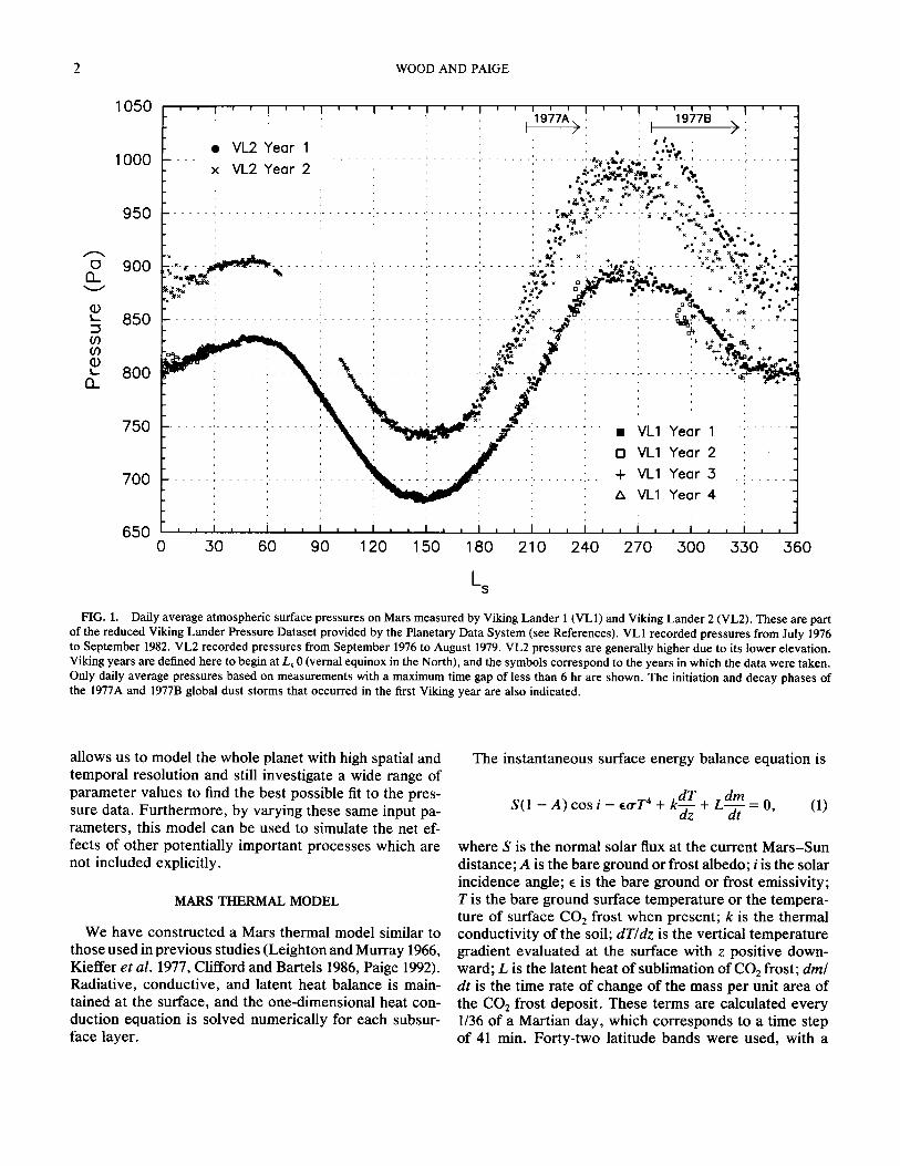
The atmospheric surface pressure records acquired at the two Viking Lander sites are extremely valuable for studying the Martian climate. These data show short time-scale fluctuations due to dynamical phenomena in the Martian atmosphere, seasonal time-scale variations due to the condensation and sublimation of carbon dioxide frost in the Martian north and south polar regions, and interannual variations due to year-to-year differences in the Martian weather and in the Martian seasonal CO2 cycle (Hess et al. 1979, Ryan and Henry 1979, Tillman et al. 1979, Leovy 1981, Leovy et al. 1985, Barnes 1980, 1981, and TiUman 1988) (Fig. 1). This seasonal cycle in-

volves a large fraction of the mass of the Martian atmo- sphere, as well as a large fraction of the surface of the planet. Any realistic model for the polar caps and atmo- sphere of Mars should at least be able to reproduce the seasonal variations exhibited by these data before at- tempting to predict the behavior of the Martian CO2 cycle during other climatic epochs.

The first serious attempt to reproduce the Viking pres- sure curves for a complete annual cycle was by James and North (1982). They employed a one-dimensional model of the North-Coakley (North et al. 1981) type, which solved for the surface heat balance as a function of lati- tude. All quantities were diurnally and zonally averaged, with an integration period of 1/200 of a Martian year. The surface was modeled as a single soil layer with a fixed heat capacity, but true subsurface heat conduction was neglected. James and North were not able to simultane- ously match the amplitudes and the relative depths of the minima of the seasonal pressure variations observed by Viking using this simple, one-dimensional model. They were, however, able to obtain a substantially better fit using a more complex, two-dimensional model that in- cluded the expected effects of global dust storms, polar hood clouds, and other atmospheric phenomena.

In this paper, we present the results of our own efforts to match the Viking Lander pressure data using a straight- forward diurnal and seasonal thermal model which in- cludes an accurate treatment of the potential effects of heat conduction. The model is similar in function to the original model developed in 1966 by Leighton and Murray (1966), which was the first to demonstrate that the advance and retreat of the seasonal polar caps on Mars can be explained by the condensation and sublimation of CO 2 frost in solid-vapor equilibrium with CO2 gas in the Mar- tian atmosphere. We find that this type of model can accurately simulate most of the major processes responsi- ble for the net heat balance of the Martian polar caps using a minimum number of input parameters. Its simplicity

0019-1035/92 $5.00 Copyright © 1992 by Academic Press, Inc.

All rights of reproduction in any form reserved.

2 WOOD A N D PAIGE

1050

1 0 0 0

950

o 900 O_

(D L 850 09 O9 @ ~-- 800

EL

750

700

6 5 0

' ' I ~ ' ! ' ' I ' ' ' ' ' ' I ' ' i , , I ' ' ; ' ' ' ' ' '

I 1977A ) I 1977B )

• VL2 Year 1 i i , t~_.),¢ : x VL2 Year 2 : : : ,; m,,~-.--.-~-.'~:"[~t"~¢~" ., ~, "t& :

. . . . . . . . . . . . ! . . . . . . . . . . . . . . : . . . . . . . . . . . . . . : . . . . . . . . . - ~ -~ ~ . . . . . :- ~. , *,.-.- ~-" . . . . : . . . . . . ' ' ' , ' ~ x , x x x ~ • ° ,

' ' *.~" . ' ~ ,.'~', 1 , , • ~ ' P . x x x , ' x , x • e .

, , , : , , ~ . , ~ . ~ . . . " , . .

¥ " ~ " " ~ . . . . . . ~ . . . . . ~ . . . . . . . . . . . . . . . . . . . . . , . . . . . . . . . . . . . . ~ - - - * J ~ * - o ' - , . . . . . , - - - . - * - - ~ - ' . - ~ - ' . - - . - I

~ , ~ . ¢ - , - , ~ , ' , , 4 . ° • . . . . ' ~ e . . ~ ? ~ . - . . " " • = " " ~ ' . . - I

%" " " ° ~ ' . "" + ~ . . . . " % • " 3 • , ' , ' , ' . . ' , . ~ . , " " ' iS. . ' . • , , ' , ' " , - , i t + , o c ~ x • . % ' 1

. . . . . . . . . . . . . . . . . . . : . . . . . . i . . . . . . . . . . . . . . . . . . . . . t , : . : ..~*" ~ : : , ~ + ÷ 1

: % . , . , : , ~ ;~ : ~ , . , + + . ~ , ~ . + . . . . ]

. . . . . . . ' . . . . . . . . . . . . " K : % . - , : , ~ y ~ ; . , , ~ . ~'Zr-~

' ' ~ - - - - ' " ' ; ~ ' ~ , * - " ~ ' ' ' 4

: , : , : . , , : , , :

. . . . . . . . . . . . . . . . . . . . . . . . . y ' i . . . . . . i • VL1 Year 1 : - i i i ~ ' : : / '. : O VL1 Yea r2 : t ~ . ~ . . _ _ j . _ _ _ ~ [ _ . ' _ . . . . . . : . . . . . . . : . . -I- ME1 Y e a r 3 : - - - - 1

Z X V L 1 Y e a r 4 t l

, , I . . . . I , , i , , I . . . . I , , i , , i , , I . . . . I

0 30 60 90 120 150 180 210 240 270 300 330 360

L s

FIG. 1. Daily average a tmospher ic surface pressures on Mars measu red by Viking Lande r 1 (VL1) and Viking Lande r 2 (VL2). These are part o f the reduced Viking L ande r Pressure Datase t provided by the Planetary Data Sys t em (see References) . V L I recorded p re s su re s f rom July 1976 to September 1982. VL2 recorded p ressures f rom September 1976 to Augus t 1979. VL2 pressures are general ly higher due to its lower elevation. Viking years are defined here to begin at L s 0 (vernal equinox in the North), and the symbols cor respond to the years in which the da ta were taken. Only daily average p ressures based on m e a s u r e m e n t s with a m a x i m u m time gap of less than 6 hr are shown. The initiation and decay phases of the 1977A and 1977B global dus t s to rms that occurred in the first Viking year are also indicated.

allows us to model the whole planet with high spatial and temporal resolution and still investigate a wide range of parameter values to find the best possible fit to the pres- sure data. Fur thermore , by varying these same input pa- rameters, this model can be used to simulate the net ef- fects of other potentially important processes which are not included explicitly.

M A R S T H E R M A L M O D E L

We have constructed a Mars thermal model similar to those used in previous studies (Leighton and Murray 1966, Kieffer et al. 1977, Clifford and Bartels 1986, Paige 1992). Radiative, conductive, and latent heat balance is main- tained at the surface, and the one-dimensional heat con- duction equation is solved numerically for each subsur- face layer.

The instantaneous surface energy balance equation is

S(1 - A) cos i - F.o'T 4 + k d T + L d m = O, dz dt

( i )

where S is the normal solar flux at the current Mars -Sun distance; A is the bare ground or frost albedo; i is the solar incidence angle; ~ is the bare ground or frost emissivity; T is the bare ground surface temperature or the tempera- ture of surface CO2 frost when present; k is the thermal conductivi ty of the soil; dT/dz is the vertical temperature gradient evaluated at the surface with z positive down- ward; L is the latent heat of sublimation of CO2 frost; d m/ dt is the time rate of change of the mass per unit area of the CO2 frost deposit. These terms are calculated every 1/36 of a Martian day, which corresponds to a time step of 41 min. For ty- two latitude bands were used, with a

FITTING THE VIKING LANDER PRESSURE CURVES 3

resolution of 2 ° near the poles and 5 ° at lower latitudes, with flat topography over the entire globe. The subsurface is divided into 40 layers of increasing thickness down to several annual skin depths. Subsurface temperatures are initialized to the estimated annual average surface temper- ature for that latitude. The one-dimensional heat conduc- tion equation

dT k d2T - ( 2 )

dt pc dz 2

is solved numerically, and the temperature of each layer is updated at time intervals which also increase with depth, but are consistent with a stable, nonoscillatory solution. We used l06 J m -3 K -1 for the product of the density p and the heat capacity c for all layers. The thermal conductivity is cast in terms of the thermal inertia, I = X/kpc, which is proportional to the heat flux in and out of the soil. The deep layers affected only by the seasonal thermal wave are assumed to have the same thermal iner- tias as layers near the surface.

The atmosphere used in our model is composed of CO2 and a small percentage (7.9 kg m -l) of noncondensible gases, and is assumed to be transparent to all radiation. Since atmospheric CO 2 is in vapor equilibrium with the seasonal frost deposits, its partial pressure determines the frost-point temperature by the solid-vapor equilibrium relation (Fanale et al. 1982). This frost-point temperature is maintained wherever any frost is on the surface by the condensation/sublimation of enough CO2 to make up any deficit/excess in the energy balance through the release/ absorption of latent heat. Since the total mass of CO2 in the cap-atmosphere system is fixed, subtracting the total CO2 condensed on the surface gives the atmospheric mass. Using a gravitational acceleration of 3.72 m sec -2, the atmospheric pressure is calculated at each time step and then used to recalculate the frost-point temperature. These adjustments can be made instantaneously because the rate at which these pressure changes are propagated is determined by the sound speed, so a disturbance can travel l0 ° of latitude in one time step and the circumfer- ence of Mars in one day.

FITTING THE VIKING LANDER PRESSURE CURVES

A. Procedure

In order to evaluate the success of our attempts to match the data, we used a smooth reference curve based on the daily average surface pressures measured by Vik- ing Lander 1 (VL1) (22.48 ° N, 47.8 ° W) (Tillman 1989). Some of the sols contained one or more data gaps lasting several hours. For our reference curve, we used daily average pressures only from those sols with a maximum time gap of less than 6 hr. The VL1 data show less suscep-

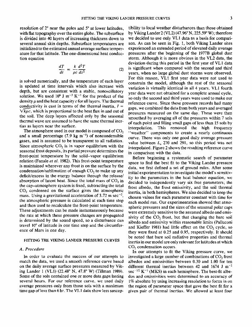
tibility to local weather disturbances than those obtained by Viking Lander 2 (VL2) (47.96 ° N, 225.59 ° W); therefore we decided to use only VL1 data as a basis for compari- son. As can be seen in Fig. 1, both Viking Lander sites experienced an extended period of elevated daily average pressures after the beginning of the 1977B global dust storm. Although it is more obvious in the VL2 data, the deviation during this period in the first year of VL1 data is significant when compared with the second and third years, when no large global dust storms were observed. For this reason, VL1 first year data were not used to constrain the model, although the rest of the seasonal variation is virtually identical in all 4 years. VL1 fourth year data were not obtained for a complete annual cycle, so only the second and third years were used to make our reference curve. Since these pressure records had many gaps, we combined the data from both years and averaged pressures measured on the same day. These were then smoothed by averaging all of the pressures within 7 sols of each point and filling small gaps of less than 15 sols by interpolation. This removed the high frequency "weather" components to create a nearly continuous curve. There was only one good daily average pressure value between L s 270 and 291, so this period was not interpolated. Figure 2 shows the resulting reference curve in comparison with the data.

Before beginning a systematic search of parameter space to find the best fit to the Viking Lander pressure data, we first defined a set of ground rules. After some initial experimentation to investigate the model's sensitiv- ity to the parameters in the heat balance equation, we decided to independently vary six free parameters; the frost albedo, the frost emissivity, and the soil thermal inertia, in both hemispheres. We also decided to keep the chosen values for each parameter constant with time for each model run. Our experimentation showed that atmo- spheric pressures and the sizes of the seasonal polar caps were extremely sensitive to the assumed albedo and emis- sivity of the CO 2 frost, but that changing the bare soil albedo and emissivity within reasonable limits (Palluconi and Kieffer 1981) had little effect on the CO2 cycle, so they were fixed at 0.25 and 0.95, respectively. It should be noted that bare soil radiative properties and thermal inertia in our model are only relevant for latitudes at which CO z condensation occurs.

In our attempts to fit the Viking pressure curve, we investigated a large number of combinations of CO 2 frost albedos and emissivities between 0.30 and 1.00 for ten different thermal inertias between 42 and 1674 J m -2 sec-l/2 K-I (MKS) in each hemisphere. The best-fit albe- dos and emissivities were determined to an accuracy of 1% absolute by using increasing resolution to focus in on the region of parameter space that gave the best fit for a given pair of thermal inertias. We allowed at least four

4 WOOD AND PAIGE

950 ' ' 1 ' ' ' ' ' 1 ' ' ' ' ! ' 1 ' ' 1 ' '

900

o 850 £L

(1) L 800

O3

L 750 rl

700

650

. . + + . . .

. . . . . . . . . . . . . . . . . . . - _ - + , ± - o ~ , !

. w

. . . . . : . . . . . . : . . . . . . . : . . . . . . . . . . . . . . . . . . . . . . . . . . . : . . . . . . . . . . . . . . . . . . . . 1 ~ : ' ' ', ' . " ' ' . "-++~ '. /

~ , : ~ : : : . : i + : : : ÷ ; \ ~ I t - - ~ , ~ . L . . . . . . ' . . . . . . . . . . . . . . . . . . . . . 1 ~ - . . . . . . . . . . . . . . . . . . . . . . . . . ". t ~ 4 z . . . . . . . : . . . . . . ! . . . . : : , . , - , , : , : ' . ' r l

. . . . . . . . . . . . . . . . . . . . . . . . . . : . . . . . . . : j "-: . . . . . . . . Reference . . . . . . .

. . . . . ': . . . . . . "- . . . . . . . . . . . . . : i ' ~ , # ~ i ~ . . . . . . . : . . . . . . . "- Vkl Yeor 3. + . " -

. . . . . . i , , , , , I . . . . . . . . i , , , , , I , ,

0 30 60 90 120 150 180 2 1 0 2 4 0 2 7 0 3 0 0 3 3 0 3 6 0

L s

FIG. 2. Comparison of the reference curve and the VL1 second and third year data (November 1977-August 1981) which were smoothed and interpolated to create it. This reference curve was used to evaluate the standard deviation of model-generated pressure curves.

Mars years for stabilization, then output the calculated daily average surface pressures and seasonal polar cap boundaries for a comple te annual cycle. Cases that yielded permanent polar caps did not converge complete ly after 4 years since the residual deposit accumulated more frost each year. Although the annual average pressures continued to fall, the shapes of the seasonal pressure variations remained the same because frost-point temper- ature depends only very weakly on vapor pressure. How- ever , these cases never resulted in a close match to the VL1 data (see Discussion and Interpretat ion, Section B). Surface pressures are calculated by our model at the alti- tude of the polar caps, which corresponds to the zero reference altitude. Since our model has n o topography, our output daily average pressures were adjusted to the measured VL1 altitude of - 1 . 5 km (Michael et al. 1976, Chris tensen 1975) using a cons tant scale height of 11.5 km (Seiff and Kirk 1977). We found that slightly changing the total mass of CO2 in the sys tem would raise or lower the annual average pressures , but it had very little effect on the shapes of the curves or the mass of the polar caps, again because it resulted in only a small change in frost- point tempera ture . For all of our model runs, we kept the total mass of CO2 fixed at 210 kg m -2, and then added or subtracted a small, constant amount of pressure to or f rom the model-calculated curves to give annual average pressures that agreed with the observat ions . We ranked

the quality of each cu rve ' s fit to the reference curve by least-squares analysis. The cases with the lowest standard deviat ion were run again, if necessary , using a total mass of CO2 which resulted in the correct annual average pres- sure. The best-fit a lbedos and emissivities were then found by checking values differing by 0.01 f rom the original set to see if a bett~r fit could be obtained using a self-consis- tent total mass of CO2.

B. Resul ts

We were able to obtain excellent fits for a wide range of model input parameters , with standard deviations of less than 10 Pa compared to an average pressure of 800 Pa. Table I lists best-fit pa rame te r values and standard deviations for several representa t ive cases. Figures 3, 4, and 5 show the pressure curves and seasonal polar cap boundaries generated by the model using these same pa- rameter values. In general, the quality of the fit increased with thermal inertia in the north, but the lowest inertias worked best in the south.

Examinat ion of our results showed that if the pa ramete r values in one hemisphere are held constant , then the best- fit frost a lbedos and emissivities in the other are linearly proport ional to the thermal inertia. I f we take the best-fit values corresponding to a thermal inertia of 1340 (MKS) in the north and 167 (MKS) in the south as a reference

FITTING THE VIKING LANDER PRESSURE CURVES

TABLE I

Best-Fit Parameter Values

Thermal Total CO2 Standard inertia Frost Frost in system deviation (MKS) albedo emissivity (kg/m 2) (Pa)

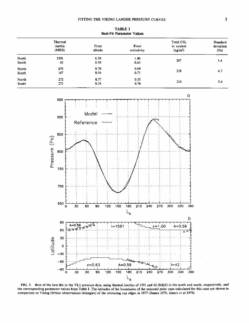
North 1591 0.59 1.00 207 3.4

South 42 0.59 0.63

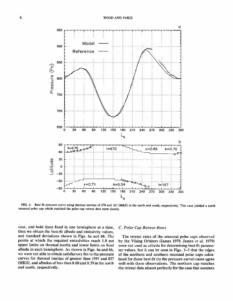
North 670 0.70 0.69 210 4.7

South 167 0.54 0.71

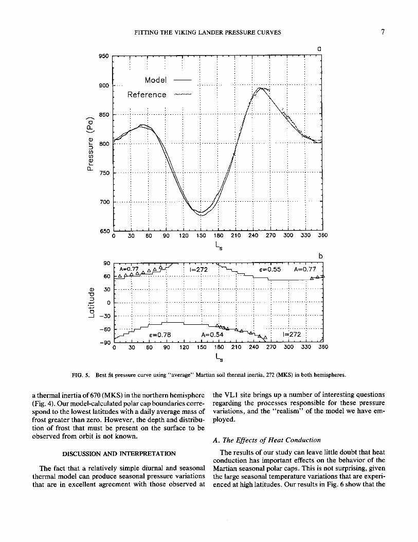
North 272 0.77 0.55 214 5.4

South 272 0.54 0.78

(3

9 5 0 / ' ' , ' • v ' • ~ ' " ~ . . . . . . . . ! . . . . . . . .

: : : ,.

M o d e l 900 . . . . . . . . . . . . . " . . . . . . . . . . . . . . : . . . . . . . . . . . . . . . : . . . . . . . : . . . .

: : i i : ~ ' : ~ .

R e f e r e n c e ............... i

. - - . . 8 5 o . . . . . . . . . . . . . . i . . . . . . . :: i . . . . . . . . . . . . . . . . . . . . . . . . . . . . . . . . . . . . :: :: i . . . . . . i ~ ~ !

rl

L 8 0 0

( / )

L .

[3_ 750

7OO

6 5 0 . . . . . . . . ; . . . . . . . . . . . . . . 0 3 0 6 0 9 0 1 2 0 1 5 0 1 8 0 2 1 0 2 4 0 2 7 0 3 0 0 3 3 0 3 6 0

Ls b

9O A - o : s 9

' ' ~ z ~ ' ' " ' . . . . . . " q 2 _ ' " ' " " ' " ' ' . . . . : j , , / ' E ~ " i ! 1 = 1 5 9 1 ~ E = I . 0 0 A = U . 5 9

6 0 - ~ - ~ ~ - - ~ . - - - - : . . . . . . . : . . . . . . . " . . . . . . -.' . . . . . . . . . . . . . . ; . . . . . . . : . . . . . . . : : A / "

3 0 . . . . . . i . . . . . . . . . . . . . . . i . . . . . . . : . . . . . . . ! . . . . . . . . . . . . . . . : . . . . . . . i . . . . . . . . . . . . . . . . . . . . . . . . . . . . . : : :

::3 0 . . . . . . . . . . . . . . . . . . . . . . . . . . . . . . . . . . . . . . . . . . . . . . . . . . . . . . . . . . . . . . . . . . . . . . . . . . . . . . . . . . . . . . . . .

o - - J - 3 0 . . . . . . . i . . . . . . . i . . . . . . ~ . . . . . . . : . . . . . . . :. . . . . . . . : . . . . . . . . . . . . . . ; . . . . . . . . . . . . . . . . . . . . . . . . . . .

i i i

- - 6 0 - - ,~- x-- . . . . ; . . . . . . . . . . . . . . . . . . . . . . . . . . . . . . ,=0.63

0 3 0 6 0 9 0 1 2 0 1 5 0 1 8 0 2 1 0 2 4 0 2 7 0 3 0 0 3 3 0 3 6 0

L s FIG. 3. Best of the best fits to the VL1 pressure data, using thermal inertias of 1591 and 42 (MKS) in the north and south, respectively, and

the corresponding parameter values from Table I. The latitudes of the boundaries of the seasonal polar caps calculated for this case are shown in comparison to Viking Orbiter observations (triangles) of the retreating cap edges in 1977 (James 1979, James et al. 1979).

6 WOOD AND PAIGE

0 Q..

(D k _

03

(D k _

EL

(D -U

E] ._1

950

900

850

800

750

700

650

90

60

.30

0

- .30

- 6 0

- 9 0

0

Cl

• • I • • ! • ' I ' ' I . . . . . . . . . . . . . . . .

: :

M o d e l . . . : . . . . . . . , . . . . . . . . . . . . . . . . . . . . . . . ! . . . . . . . : . . . . . . . ~ . . . .

R e f e r e n c e ............... ~ ::

• , . , ' .

. . . . . i . . . . . . . i . . . . . . . ! . . . . . . . i . . . . . . . . . . . . . . . . . . . . . . . . . . . . . . . . . .

i : ', : ' ' % '. • : : . . . ~ :

: : : : : ?%,:

`30 60 90 120 150 180 210 240 270 `300 330 .360

Ls

b ' A ~ 0 . 7 0 ' i • • i ~ ' ~ ~ . ~ ! • • i • • i . . . . ~ _ . ~ i , , i , i ' • i • , i ' ' i ' '

. A : : ----670 : "~'-n___ ~=0.69 A----0.70 ~ . i . . . . . . . ! . . . . . . . i . . . . . . " . . . . . . . . . . . . . . i . . . . . .

. . . . . . i . . . . . . . i . . . . . . . ~. . . . . . . . : . . . . . . . . . . . . . . . . . . . . . . . . . . . . . . . . . . . . . . . . . . . . . . . . . . . . . . . . .

~E=0.71 , , I • I I , , I , , I

0 30 60 90 120

. . . . : . . . . . . . . . . . . . . . . . . . . . . . , . . . . . . . . . . . . . . . . . . . . . . . . . . . . .

. . . . . , I , , I , \ , ' , , i , = ' , ,

150 180 210 240 270 300 .330 36(

L s

FIG. 4. Best fit pressure curve using thermal inertias of 670 and 167 (MKS) in the north and south, respectively. This case yielded a north seasonal polar cap which matched the polar cap retreat data most closely.

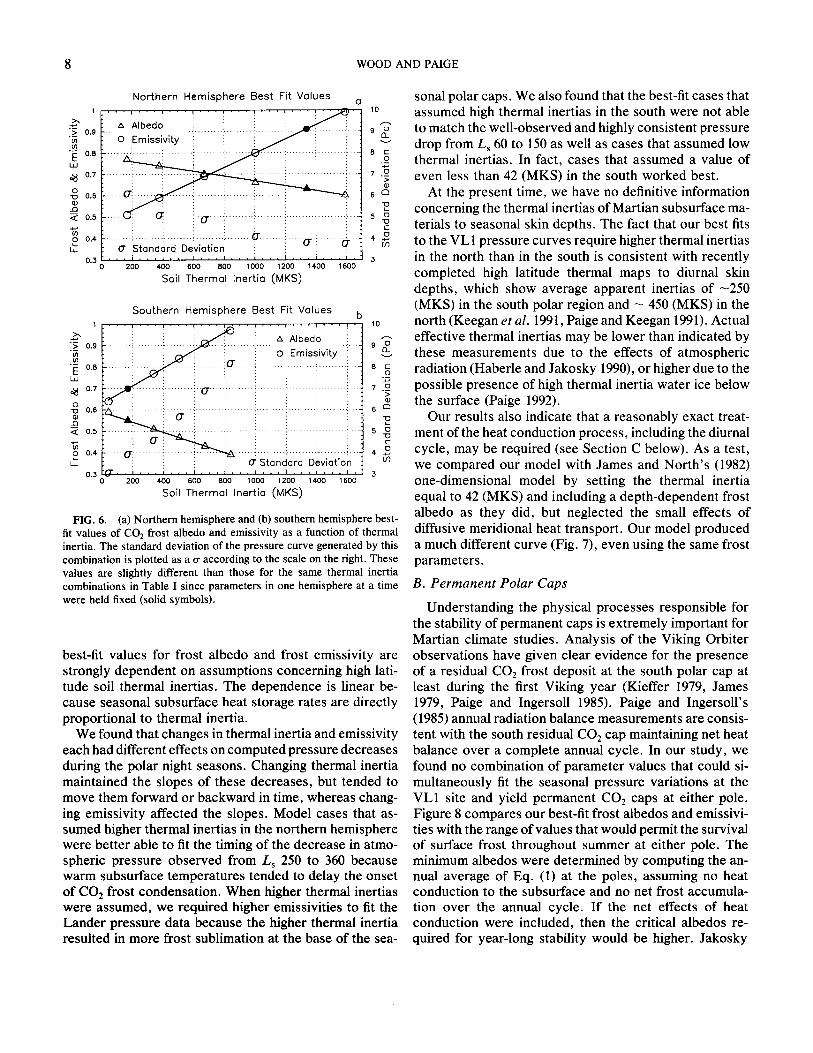
case, and hold them fixed in one hemisphere at a time, then we obtain the best-fit albedo and emissivity values, and standard deviations shown in Figs. 6a and 6b. The points at which the required emissivities reach 1.0 put upper limits on thermal inertia and lower limits on frost albedo in each hemisphere. As shown in Figs. 6a and 6b, we were not able to obtain satisfactory fits to the pressure curves for thermal inertias of greater than 1591 and 837 (MKS), and albedos of less than 0.60 and 0.39 in the north and south, respectively.

C. Polar Cap Retreat Rates

The retreat rates of the seasonal polar caps observed by the Viking Orbiters (James 1979, James et al. 1979) were not used as criteria for determining best-fit parame- ter values, but it can be seen in Figs. 3-5 that the edges of the northern and southern seasonal polar caps calcu- lated for these best-fit (to the pressure curve) cases agree well with these observations. The northern cap matches the retreat data almost perfectly for the case that assumes

FITTING THE VIKING LANDER PRESSURE CURVES 7

O £L

(1) k_ "-I

(/)

k_ £L

FIG. 5.

"0

._J

950

900

850

800

750

700

650

90

60

30

0

- 3 0

- 6 0

- 9 0 0

(3 • , u • , ! ' • I ' ' I . . . . . . . . . . . . . . .

:

M o d e l

R e f e r e n c e ............... ~ i

. . . . . ! . . . . . . . i . . . . . . . i . . . . . . . i . . . . . . . . . . . . . . . . . . . . . . . . . . . .~. . . . . . . . . . . . . .

.. . : , : : : . , ~ :

, , . : : . ~ , . : , , . : . . , ~ . : . , .

: : i i : : I ; : i : : • ' . . , , t * . . ' : , , , ' s : . . . .

i i . . . . . . i . . . . I , , , , , . i . . . .

0 30 60 90 120 150 180 210 240 270 300 330 360

I- s

• ' I ' ' I ' • I • • . i . . . . I ' ' I ' ' I • •

A=0.77 i ~ 1=272 " ~ ' L L ' ~ ' E=0.55 . , , ¢~ ~ " ~ - - ! . . . . . . . . . . . . . . . . . . . . . . '.. . . . . .

t

. . . . . . i . . . . . . . i . . . . . . . . . . . . . . . . . . . . . . . . . . . . . . . . . . . . . . . . . . . . . . . . . . . . . . . . . . . . . . . . . . . . . . . . . . . .

. . . . . . i . . . . . . . ; . . . . . . i . . . . . . . i . . . . . . . . . . . . . . . . . . . . . . . i . . . . . . . . . . . . . . . . . . . . . . . . . . . . . . . . . . . . . . .

b

'A;c;.77'

~ : : I A~^i, ^

" ; - - 0 . p , , , , , °, . : . . . . . . . : . . . . . . . . . . . . . . . . . . . . . , .

30 60 90 120 150 180 210 240 270 300 330 360

L s

Best fit pressure curve using "ave rage" Martian soil thermal inertia, 272 (MKS) in both hemispheres .

a thermal inertia of 670 (MKS) in the northern hemisphere (Fig. 4). Our model-calculated polar cap boundaries corre- spond to the lowest latitudes with a daily average mass of frost greater than zero. However, the depth and distribu- tion of frost that must be present on the surface to be observed from orbit is not known.

DISCUSSION AND INTERPRETATION

The fact that a relatively simple diurnal and seasonal thermal model can produce seasonal pressure variations that are in excellent agreement with those observed at

the VL1 site brings up a number of interesting questions regarding the processes responsible for these pressure variations, and the "real ism" of the model we have em- ployed.

A. The Effects of Heat Conduction

The results of our study can leave little doubt that heat conduction has important effects on the behavior of the Martian seasonal polar caps. This is not surprising, given the large seasonal temperature variations that are experi- enced at high latitudes. Our results in Fig. 6 show that the

8 WOOD AND PAIGE

I

i~ 0.9

"~ 0.8

ILl ,.8 0.7

~ O 0.6

~< 0.5

O 0.4 t a _

0 . 3

N o r t h e r n H e m i s p h e r e Bes t Fit Va lues a

• ; 0ado . . . , . . .

'"""" " 5 : ' ' O" i 4

. . . . . . . . . ' . . . . . . . . . . : . . . . . . . . : ' : : (7 : CT Standard Deviation i i i :

• . . i . , . t . . , I , , . i . . . I . . . I . • • . • • • I . 3

200 400 600 aoo ~ooo 12oo 14oo 16oo

Soil Thermal Inertia (MKS)

10

8 E 0

~.~

7 . N

6 C 2 1

o

2 [ / 3

S o u t h e r n H e m i s p h e r e Bes t Fit Va lues b 1 . . . . . . i • . . ! . . . i . • • i • • • i ' ' ' i . , , ! ,

"~ 0 .9 . . . . . . . . . . . . . . . . : . . . . . . . . . . . . . . . . ; . . . . . . . . .i . . . . 0 E m s s : v ;*'',,~y ! . . . .

• ~: 0.8 ....... ......... ........ ......... ..... : ................ i ......... ~ .....

,~ 0.7 .................................

0

. . . . . . . . . . . . . . . . . . . . . . . . . . . . . . . ................................ ! ........... : ................ i o 0., .... i i , ........ i , , , i o , u_ i 0 . 3 v

0 200 4oo 600 soo i000 1200 1400 isoo

Soil Thermal Inertia (MKS)

1 0

9 ~

7 ~

6 ¢ ~

E

4 ~ ( 1 3

3

FIG. 6. (a) Northern hemisphere and (b) southern hemisphere best- fit values of CO2 frost albedo and emissivity as a function of thermal inertia. The standard deviation of the pressure curve generated by this combination is plotted as a o- according to the scale on the right. These values are slightly different than those for the same thermal inertia combinations in Table I since parameters in one hemisphere at a time were held fixed (solid symbols).

best-fit values for frost albedo and frost emissivity are strongly dependent on assumptions concerning high lati- tude soil thermal inertias. The dependence is linear be- cause seasonal subsurface heat storage rates are directly proport ional to thermal inertia.

We found that changes in thermal inertia and emissivity each had different effects on computed pressure decreases during the polar night seasons. Changing thermal inertia maintained the slopes of these decreases, but tended to move them forward or backward in time, whereas chang- ing emissivity affected the slopes. Model cases that as- sumed higher thermal inertias in the northern hemisphere were bet ter able to fit the timing of the decrease in atmo- spheric pressure observed from L s 250 to 360 because warm subsurface temperatures tended to delay the onset of CO2 frost condensation. When higher thermal inertias were assumed, we required higher emissivities to fit the Lander pressure data because the higher thermal inertia resulted in more frost sublimation at the base of the sea-

sonal polar caps. We also found that the best-fit cases that assumed high thermal inertias in the south were not able to match the well-observed and highly consistent pressure drop from L~ 60 to 150 as well as cases that assumed low thermal inertias. In fact, cases that assumed a value of even less than 42 (MKS) in the south worked best.

At the present time, we have no definitive information concerning the thermal inertias of Martian subsurface ma- terials to seasonal skin depths. The fact that our best fits to the VL1 pressure curves require higher thermal inertias in the north than in the south is consistent with recently completed high latitude thermal maps to diurnal skin depths, which show average apparent inertias of - 2 5 0 (MKS) in the south polar region and - 450 (MKS) in the north (Keegan e t a l . 1991, Paige and Keegan 1991). Actual effective thermal inertias may be lower than indicated by these measurements due to the effects of atmospheric radiation (Haberle and Jakosky 1990), or higher due to the possible presence of high thermal inertia water ice below the surface (Paige 1992).

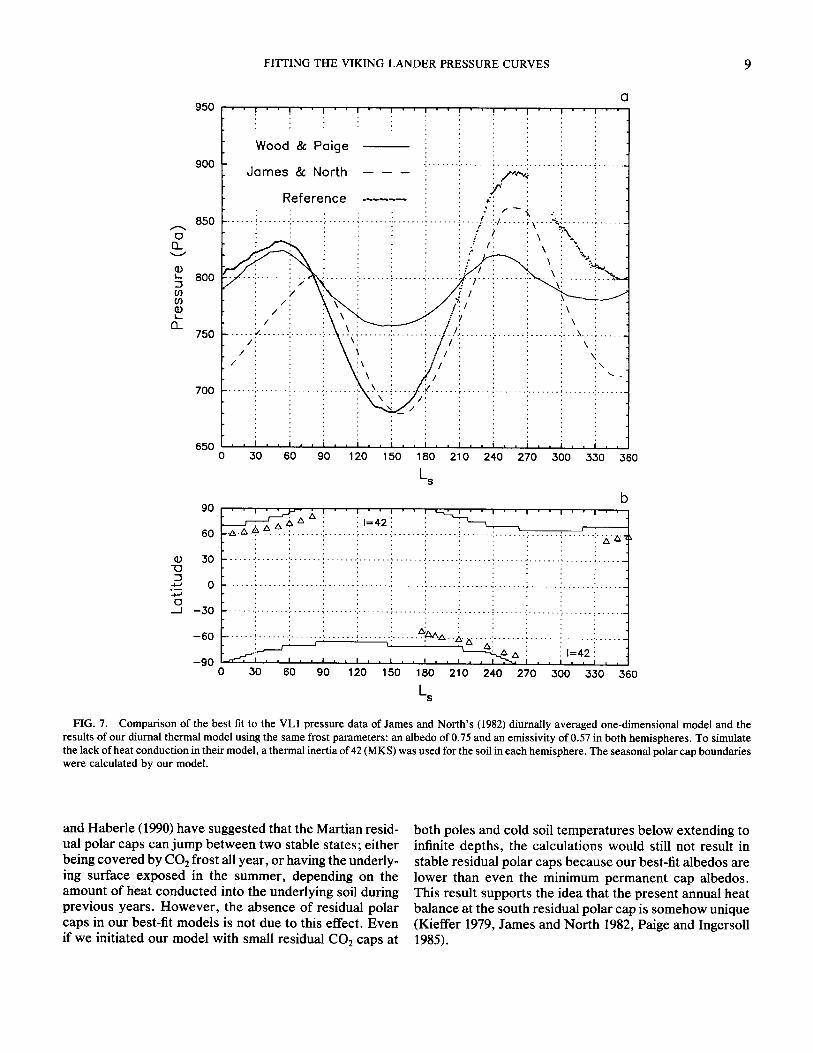
Our results also indicate that a reasonably exact treat- ment of the heat conduct ion process, including the diurnal cycle, may be required (see Section C below). As a test, we compared our model with James and Nor th ' s (1982) one-dimensional model by setting the thermal inertia equal to 42 (MKS) and including a depth-dependent frost albedo as they did, but neglected the small effects of diffusive meridional heat transport. Our model produced a much different curve (Fig. 7), even using the same frost parameters.

B . P e r m a n e n t P o l a r C a p s

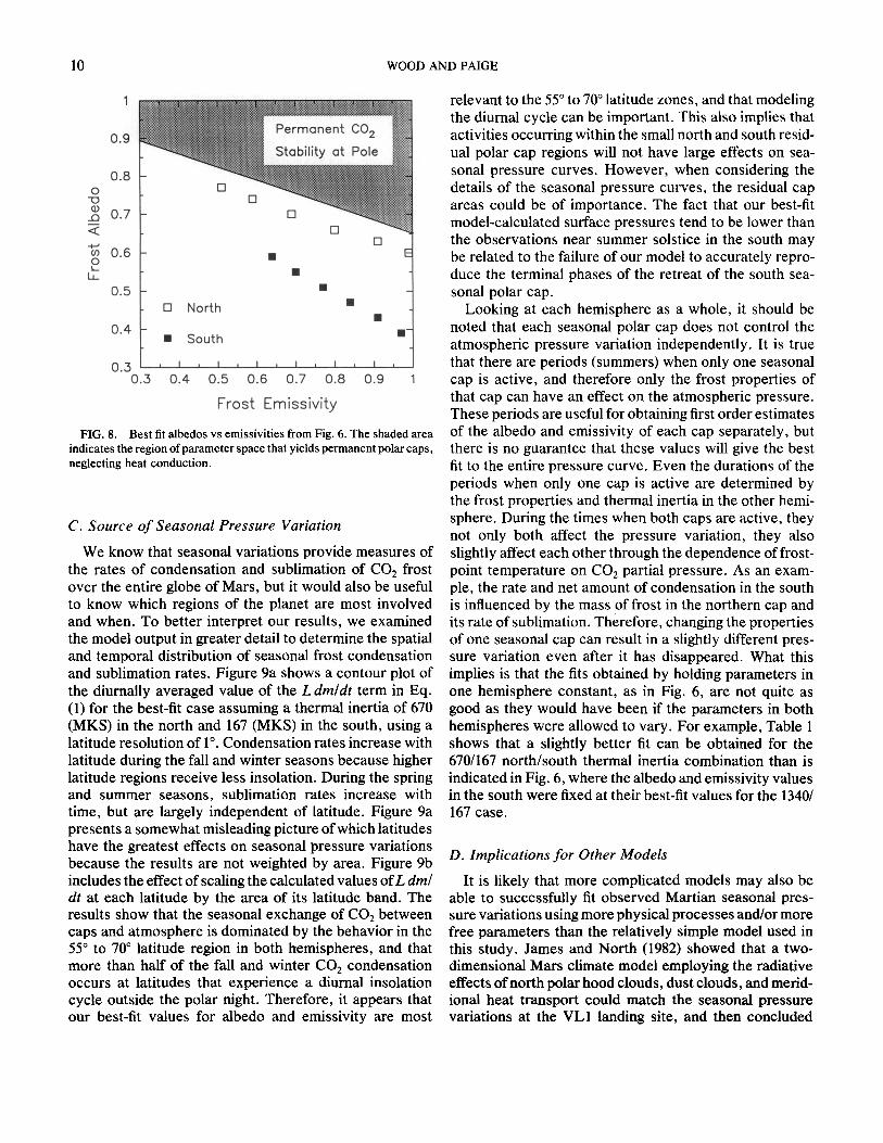
Understanding the physical processes responsible for the stability of permanent caps is extremely important for Martian climate studies. Analysis of the Viking Orbiter observations have given clear evidence for the presence of a residual CO2 frost deposit at the south polar cap at least during the first Viking year (Kieffer 1979, James 1979, Paige and Ingersoll 1985). Paige and Ingersoll 's (1985) annual radiation balance measurements are consis- tent with the south residual COz cap maintaining net heat balance over a complete annual cycle. In our study, we found no combination of parameter values that could si- multaneously fit the seasonal pressure variations at the VL1 site and yield permanent CO2 caps at either pole. Figure 8 compares our best-fit frost albedos and emissivi- ties with the range of values that would permit the survival of surface frost throughout summer at either pole. The minimum albedos were determined by computing the an- nual average of Eq. (1) at the poles, assuming no heat conduct ion to the subsurface and no net frost accumula- tion over the annual cycle. If the net effects of heat conduct ion were included, then the critical albedos re- quired for year-long stability would be higher. Jakosky

FITTING THE VIKING LANDER PRESSURE CURVES 9

0 EL

© L .

U) ( 0

L_ EL

"U

0

950

900

8 5 0

800

750

7 0 0

6 5 0

90

60

30

0

- 3 0

- 6 0

- 9 0

' ! ' " ! " ' I ' '

W o o d & P a i g e

d o m e s & N o r t h

R e f e r e n c e

• • i ' '

o . . . . ! . . . . . . . .

. / : g : :

. . . . . . :i ............... :~ .... . . . . . . . . . . . . . . . . . . . . . . . . . . . . . .: ¢: i " . . . . . - ~ s, . : .... : \ . . . . ;: . . . . . . . . • : \ :'N : , : : :' , . % :

i : .~ / : : \ \ . i ~ • . ' ~ . . . . ~

• : > . . . . . . :: . . . . . . . i . . . . . . . i . . . . . . . . . . . ~ . . . . . . i . . . . .

: / : ' . \ \ ~ : : ' ~ / i - , ' i : : \ i - i i i , i .

. . . . . . . : . . . . . . . : . . . . . . . : . . . . . . . :. , : . . . ~ . . . . . . : . . . . . . . . . . . . : . . . . . . .

:

i i

30 60 90 120 150 180 210 240 270 300 330 360

I- s

b ' ' i . . . . i • • i • , i . . . . . . . . . . . . .

! , = , 2 ! ' ' '

_~.tx ~ . . . . . . ; . . . . . . . : . . . . . . . ! . . . . . . ! . . . . . . . . . . . . . . . . . . . . . . ~ . . . . . . . . . . . . . . . . . . . . . . . " x ~ '

l

. . . . . . : . . . . . . . i . . . . . . . '. . . . . . . . ; . . . . . . . .~ . . . . . . . . . . . . . . . . . . . . . . . . . . . . . . . . . . . . . . . . . . . . . . . . . . . .

. . . . . . ~ . . . . . . i . . . . . . . ! . . . . . . . : . . . . . . . i . . . . . . . ~ . . . . . . ~ . . . . . . . . . . . . . . . . . . . . . . . . . . . . . . . . . . . . .

. . . . . . . ! . . . . . . . ; . . . . . . i . . . . . . . i . . . . . . . ; . . . . . . . i . . . . . . . i . . . . . . . . . . . . . . . . . . . . . . . . . . . . . . . . . . .

. . . . : i i .- --! . . . . . . . ; . . . . . ;-,

" ~ l w = |

0 30 60 90

: i i i ~ , , , , . . . . . Z~" ~ / . . . . ', . . . . . . . : . . . . . . . '. . . . . . . . '. . . . . . . -£----_ . . . . ~ ~ . . . 1 = 4 2 A

i . I I . , i . . i , , ! I"-%, , , . , i i

120 150 180 210 240 270 300 330 360

L s

FIG. 7. Comparison of the best fit to the VLI pressure data of James and North's (1982) diurnally averaged one-dimensional model and the results of our diurnal thermal model using the same frost parameters: an aibedo of 0.75 and an emissivity of 0.57 in both hemispheres. To simulate the lack of heat conduction in their model, a thermal inertia of 42 (MKS) was used for the soil in each hemisphere. The seasonal polar cap boundaries were calculated by our model.

a n d H a b e r l e (1990) h a v e s u g g e s t e d t h a t t h e M a r t i a n r e s id -

ua l p o l a r c a p s c a n j u m p b e t w e e n t w o s t a b l e s t a t e s ; e i t h e r

b e i n g c o v e r e d b y CO2 f r o s t al l y e a r , o r h a v i n g t h e u n d e r l y -

i ng s u r f a c e e x p o s e d in t h e s u m m e r , d e p e n d i n g o n t h e a m o u n t o f h e a t c o n d u c t e d i n t o t h e u n d e r l y i n g soi l d u r i n g

p r e v i o u s y e a r s . H o w e v e r , t h e a b s e n c e o f r e s i d u a l p o l a r

c a p s in o u r bes t - f i t m o d e l s is n o t d u e to th is e f f e c t . E v e n

i f w e i n i t i a t e d o u r m o d e l w i t h s m a l l r e s i d u a l CO2 c a p s a t

b o t h p o l e s a n d c o l d so i l t e m p e r a t u r e s b e l o w e x t e n d i n g to

in f in i te d e p t h s , t h e c a l c u l a t i o n s w o u l d st i l l n o t r e s u l t in

s t a b l e r e s i d u a l p o l a r c a p s b e c a u s e o u r bes t - f i t a l b e d o s a r e

l o w e r t h a n e v e n t h e m i n i m u m p e r m a n e n t c a p a l b e d o s . T h i s r e s u l t s u p p o r t s t h e i d e a t h a t t h e p r e s e n t a n n u a l h e a t

b a l a n c e a t t h e s o u t h r e s i d u a l p o l a r c a p is s o m e h o w u n i q u e

( K i e f f e r 1979, J a m e s a n d N o r t h 1982, P a i g e a n d I n g e r s o l l 1985).

10 WOOD AND PAIGE

0

(D

< :

03 0 k_

t,

1 I 0.9

0.8

0.7

0.6

0.5

0.4

0.3 - 0.3

Permonent CO 2

Stability ot Pole

[ ] [ ]

13 [ ]

[ ]

[] North •

• South

0.4 0.5 0.6 0.7 0.8 0.9

F r o s t Emissivity

FIG. 8. Best fit albedos vs emissivities from Fig. 6. The shaded area indicates the region of parameter space that yields permanent polar caps, neglecting heat conduction.

C. Source of Seasonal Pressure Variation

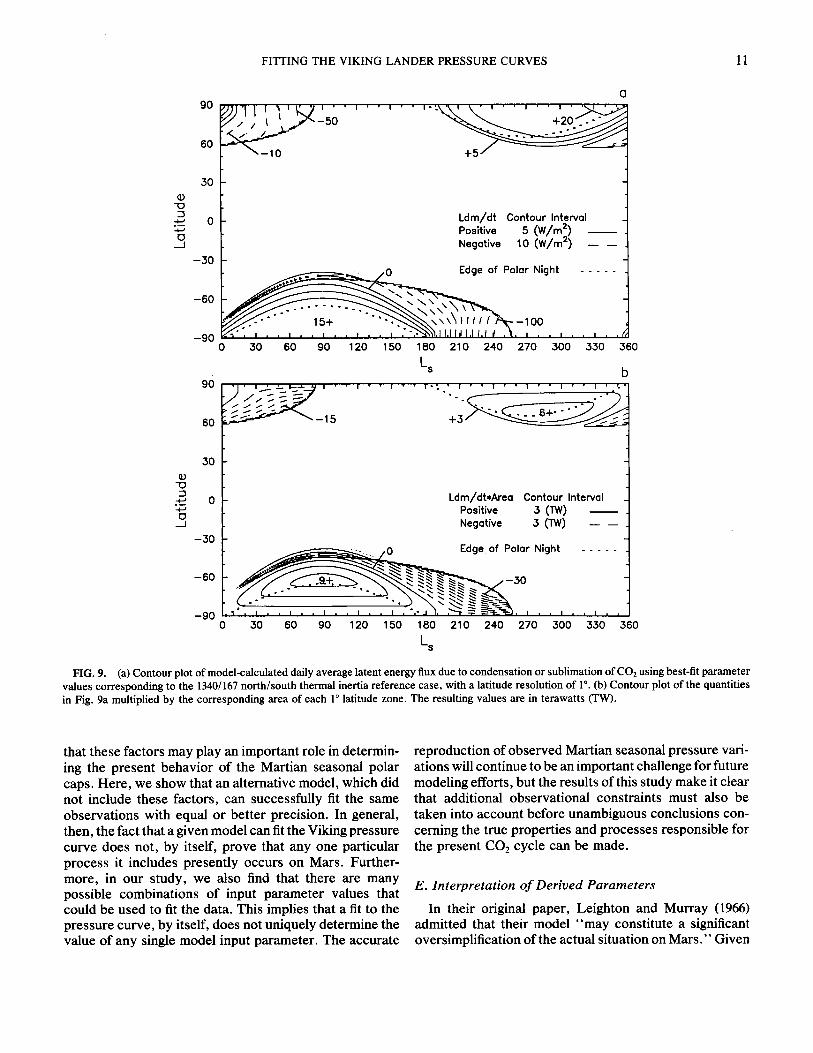
We know that seasonal variations provide measures of the rates of condensation and sublimation of CO 2 frost over the entire globe of Mars, but it would also be useful to know which regions of the planet are most involved and when. To better interpret our results, we examined the model output in greater detail to determine the spatial and temporal distribution of seasonal frost condensation and sublimation rates. Figure 9a shows a contour plot of the diurnally averaged value of the L dm/dt term in Eq. (1) for the best-fit case assuming a thermal inertia of 670 (MKS) in the north and 167 (MKS) in the south, using a latitude resolution of 1 °. Condensation rates increase with latitude during the fall and winter seasons because higher latitude regions receive less insolation. During the spring and summer seasons, sublimation rates increase with time, but are largely independent of latitude. Figure 9a presents a somewhat misleading picture of which latitudes have the greatest effects on seasonal pressure variations because the results are not weighted by area. Figure 9b includes the effect of scaling the calculated values ofL dm/ dt at each latitude by the area of its latitude band. The results show that the seasonal exchange of CO2 between caps and atmosphere is dominated by the behavior in the 55 ° to 70 ° latitude region in both hemispheres, and that more than half of the fall and winter CO 2 condensation occurs at latitudes that experience a diurnal insolation cycle outside the polar night. Therefore, it appears that our best-fit values for albedo and emissivity are most

relevant to the 55 ° to 70 ° latitude zones, and that modeling the diurnal cycle can be important. This also implies that activities occurring within the small north and south resid- ual polar cap regions will not have large effects on sea- sonal pressure curves. However, when considering the details of the seasonal pressure curves, the residual cap areas could be of importance. The fact that our best-fit model-calculated surface pressures tend to be lower than the observations near summer solstice in the south may be related to the failure of our model to accurately repro- duce the terminal phases of the retreat of the south sea- sonal polar cap.

Looking at each hemisphere as a whole, it should be noted that each seasonal polar cap does not control the atmospheric pressure variation independently. It is true that there are periods (summers) when only one seasonal cap is active, and therefore only the frost properties of that cap can have an effect on the atmospheric pressure. These periods are useful for obtaining first order estimates of the albedo and emissivity of each cap separately, but there is no guarantee that these values will give the best fit to the entire pressure curve. Even the durations of the periods when only one cap is active are determined by the frost properties and thermal inertia in the other hemi- sphere. During the times when both caps are active, they not only both affect the pressure variation, they also slightly affect each other through the dependence of frost- point temperature on CO2 partial pressure. As an exam- ple, the rate and net amount of condensation in the south is influenced by the mass of frost in the northern cap and its rate of sublimation. Therefore, changing the properties of one seasonal cap can result in a slightly different pres- sure variation even after it has disappeared. What this implies is that the fits obtained by holding parameters in one hemisphere constant, as in Fig. 6, are not quite as good as they would have been if the parameters in both hemispheres were allowed to vary. For example, Table 1 shows that a slightly better fit can be obtained for the 670/167 north/south thermal inertia combination than is indicated in Fig. 6, where the albedo and emissivity values in the south were fixed at their best-fit values for the 1340/ 167 case.

D. Implications for Other Models

It is likely that more complicated models may also be able to successfully fit observed Martian seasonal pres- sure variations using more physical processes and/or more free parameters than the relatively simple model used in this study. James and North (1982) showed that a two- dimensional Mars climate model employing the radiative effects of north polar hood clouds, dust clouds, and merid- ional heat transport could match the seasonal pressure variations at the VL1 landing site, and then concluded

FITTING THE VIKING LANDER PRESSURE CURVES 11

60

30

% 2

.% 0 Ldm/dt Contour lntervol

5 Negative 10 (W/m’) - -

-30 Edge of Polar Night - - - - -

-60

-90 0 30 60 90 120 150 160 210 240 270 300 330 360

90

60

30

: .z 0 Ldm/dt*Area Contour Interval

4

-30 Edge of Polar Night - - - - -

-60

-90 0 30 60 90 120 150 180 210 240 270 300 330 360

Ls

FIG. 9. (a) Contour plot of model-calculated daily average latent energy flux due to condensation or sublimation of CO2 using best-fit parameter values corresponding to the 1340/167 north/south thermal inertia reference case, with a latitude resolution of 1”. (b) Contour plot of the quantities in Fig. 9a multiplied by the corresponding area of each 1” latitude zone. The resulting values are in terawatts (TW).

that these factors may play an important role in determin- ing the present behavior of the Martian seasonal polar caps. Here, we show that an alternative model, which did not include these factors, can successfully fit the same observations with equal or better precision. In general, then, the fact that a given model can fit the Viking pressure curve does not, by itself, prove that any one particular process it includes presently occurs on Mars. Further- more, in our study, we also find that there are many possible combinations of input parameter values that could be used to fit the data. This implies that a fit to the pressure curve, by itself, does not uniquely determine the value of any single model input parameter. The accurate

reproduction of observed Martian seasonal pressure vari- ations will continue to be an important challenge for future modeling efforts, but the results of this study make it clear that additional observational constraints must also be taken into account before unambiguous conclusions con- cerning the true properties and processes responsible for the present CO2 cycle can be made.

E. Interpretation of Derived Parameters

In their original paper, Leighton and Murray (1966) admitted that their model “may constitute a significant oversimplification of the actual situation on Mars.” Given

12 W O O D A N D P A I G E

950

9 0 0

850 13_

©

L 800 "-i 03 03

Q _ 7 5 0

700

650

With Dust S t o r m s . . . . ! .

" ' " W / o u t Ous t S t o r m s - - . ' : . . . . . . ~ : ~ . . . . : . . . . . . . : . . . . . . r

VL1 Y e a r 1 D a t a . , . . . - 1 , . :: ~ ~ . ~ , ::

. . . . . :: . . . . . . : . . . . . . . i . . . . . . z . . . . . . i . . . . . . . . . . . . . i . . . . . ' . . . . i . . . . . . !

7

. . . . . . ) . . : . . . . . . . . . . . . . . : . . . . . . ! . . . . . . ~. . . . . . . . •

/ ' , .. , '. : , N : " . . i i . " ~ " i : : : : ! : : : . : " :

. . . . . . . . I , , I . . . . . . . i i i i i i i

0 30 60 90 120 150 180 210 240 270 300 330 360

L s

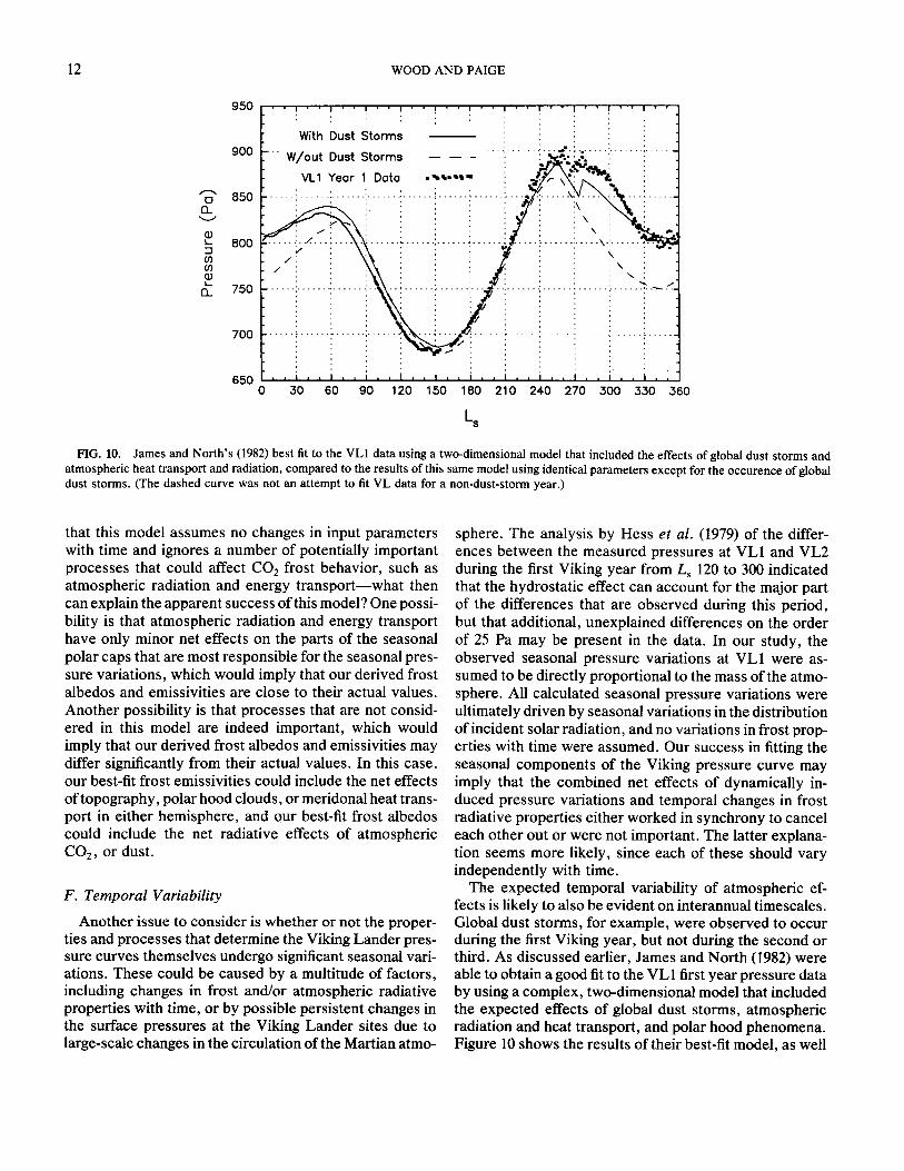
FIG. 10. James and North's (1982) best fit to the VL1 data using a two-dimensional model that included the effects of global dust storms and atmospheric heat transport and radiation, compared to the results of this same model using identical parameters except for the occurence of global dust storms. (The dashed curve was not an attempt to fit VL data for a non-dust-storm year.)

that this model assumes no changes in input parameters with time and ignores a number of potentially important processes that could affect C02 frost behavior, such as atmospheric radiation and energy transport--what then can explain the apparent success of this model? One possi- bility is that atmospheric radiation and energy transport have only minor net effects on the parts of the seasonal polar caps that are most responsible for the seasonal pres- sure variations, which would imply that our derived frost albedos and emissivities are close to their actual values. Another possibility is that processes that are not consid- ered in this model are indeed important, which would imply that our derived frost albedos and emissivities may differ significantly from their actual values. In this case, our best-fit frost emissivities could include the net effects of topography, polar hood clouds, or meridonal heat trans- port in either hemisphere, and our best-fit frost albedos could include the net radiative effects of atmospheric C02, or dust.

F. Temporal Variability

Another issue to consider is whether or not the proper- ties and processes that determine the Viking Lander pres- sure curves themselves undergo significant seasonal vari- ations. These could be caused by a multitude of factors, including changes in frost and/or atmospheric radiative properties with time, or by possible persistent changes in the surface pressures at the Viking Lander sites due to large-scale changes in the circulation of the Martian atmo-

sphere. The analysis by Hess et al. (1979) of the differ- ences between the measured pressures at VL1 and VL2 during the first Viking year from Ls 120 to 300 indicated that the hydrostatic effect can account for the major part of the differences that are observed during this period, but that additional, unexplained differences on the order of 25 Pa may be present in the data. In our study, the observed seasonal pressure variations at VL1 were as- sumed to be directly proportional to the mass of the atmo- sphere. All calculated seasonal pressure variations were ultimately driven by seasonal variations in the distribution of incident solar radiation, and no variations in frost prop- erties with time were assumed. Our success in fitting the seasonal components of the Viking pressure curve may imply that the combined net effects of dynamically in- duced pressure variations and temporal changes in frost radiative properties either worked in synchrony to cancel each other out or were not important. The latter explana- tion seems more likely, since each of these should vary independently with time.

The expected temporal variability of atmospheric ef- fects is likely to also be evident on interannual timescales. Global dust storms, for example, were observed to occur during the first Viking year, but not during the second or third. As discussed earlier, James and North (1982) were able to obtain a good fit to the VL1 first year pressure data by using a complex, two-dimensional model that included the expected effects of global dust storms, atmospheric radiation and heat transport, and polar hood phenomena. Figure 10 shows the results of their best-fit model, as well

FITTING THE VIKING LANDER PRESSURE CURVES 13

as the results of their model using identical parameters with the exception of dust storm effects (James and North 1982). As can be seen in the figure, James and North's two-dimensional model appears to rely heavily on the effects of the dust storm itself in order to fit the VL1 first year data. To match the pressure minima around L S 360, which is nearly the same in all 3 years, their model would require a different set of atmospheric effects. One com- mon aspect of the James and North best-fit model results and our own is the need for a heat source in the north polar region to delay the onset of frost condensation in fall, and to reduce net frost condensation rates during fall and winter. In our model, this heat source is not due to dynamic and radiative processes occurring in the atmo- sphere, but to heat conduction from the subsurface. Of the two, subsurface heat conduction would be expected to exhibit the least interannual variability, and thus may help to explain the interannual repeatability of the Viking Lander seasonal pressure variations.

G. Potential Applications

The present CO 2 cycle on Mars is a complex and sensi- tive system. In many investigations of the atmosphere, surface, and subsurface of Mars, it is desirable to have a conceptually simple, computationally efficient, and physi- cally based model that fits the Viking Lander pressure curve and the seasonal polar cap retreat data. For prob- lems that require knowledge of the mass of CO2 on the surface, or the rates of CO2 condensation or sublimation, at any given place and time, our model can provide esti- mates of these quantities that are consistent with available observations. The model should also be useful for study- ing the effects of global dust storms, the long-term stability of permanent polar caps, and the sensitivity of the sea- sonal cycle to variations in the orbital and axial elements of Mars.

C O N C L U S I O N S

This investigation has shown that: 1. It is possible to fit the seasonal component of the

Viking Lander pressure variations to within a few pascal using a diurnal and seasonal thermal model without any explicit atmospheric contributions to the heat balance, and parameters that are kept constant with time.

2. Although the best-fit model parameter values are not unique, there is a fixed relationship between them, so that if one is specified, the others are determined.

3. Subsurface heat conduction has significant effects on Martian seasonal pressure variations, polar cap bound- aries, and best-fit frost albedos and emissivities. It can provide a means of influencing frost accumulation rates that is highly repeatable from year to year.

4. Seasonal pressure variations are dominated by the heat balance of the 55 ° to 70 ° latitude zone in both hemi- spheres. Thus, almost all of the most influential portions of the seasonal polar caps receive some sunlight through- out the winter.

5. The albedo and emissivity values required to fit the pressure curve with the model used in this study are not consistent with the stability of permanent CO2 deposits at either pole, even if the model is initialized with a cold subsurface. This implies that the heat balance of the sea- sonal frost deposits at the south residual cap differs from that of the most influential portions of the south seasonal cap.

A C K N O W L E D G M E N T S

We thank J. E. Tillman, the Viking Lander Meteorology Team, and the Planetary Data System for supplying us with these invaluable data, and P. B. James and R. W. Zurek for helpful reviews of this manuscript. This work was supported by the NASA Mars Surface and Atmosphere Through Time Program.

R E F E R E N C E S

BARNES, J. R. 1980. Time spectral analysis of midlatitude disturbances in the Martian atmosphere. J. Atmos. Sci. 37, 2002-2015.

BARNES, J. R. 1981. Midlatitude disturbances in the Martian atmosphere: A second Mars year. J. Atmos. Sci. 38, 225-234.

CHRISTENSEN, E. J. 1975. Martian topography derived from occultation, radar, spectral, and optical measurements. J. Geophys. Res. 80, 2909-2913.

CLIFFORD, S. M., AND C. J. BARTELS 1986. The Mars thermal model (MARSTHERM): A Fortran 77 finite-difference program designed for general distribution. Proc. Lunar Planet Sci. Conf. 17th, 142-143.

FANALE, F. P., J. R. SALVAIL, W. B. BANERDT, AND R. S. lAUNDERS 1982. Mars: The regoli th-atmosphere-cap system and climate change. Icarus 50, 381-407.

HABERLE, R. M. AND B. M. JAKOSKY 1991. Atmospheric effects on the remote determination of thermal inertia on Mars. Icarus 90, 187-204.

HESS, S. L., R. M. HENRY, AND J. E. TILLMAN 1979. The seasonal variation of atmospheric pressure on Mars as affected by the South Polar Cap. J. Geophys. Res. 84, 2923-2927.

JAKOSKY, B. M., AND R. M. HABERLE 1990. Year-to-year instability of the Mars South Polar Cap. J. Geophys. Res. 95, 1359-1365.

JAMES, P. B. 1979. Recession of Martian North Polar Cap: 1977-1978 Viking observations. J. Geophys. Res. 84, 8332-8334.

JAMES, P. B., G. BRIGGS, J. BARNES, AND A. SPRUCK 1979. Seasonal recession of Mars' South Polar Cap as seen by Viking. J. Geophys. Res. 84, 2889-2922.

JAMES. P. B., AND G. R. NORTH 1982. The seasonal cycle of CO 2 on Mars: An application of an energy balance climate model. J. Geophys. Res. 87, 10271-10283.

KEEGAN, K .D., J. E. BACHMAN, AND D. A. PAIGE 1991. Thermal and albedo mapping of the North Polar Region of Mars. Lunar Planet. Sci. XXII, 701-702.

KIEFFER, H. H. 1979. Mars south polar spring and summer tempera- tures: A residual CO 2 frost. J. Geophys. Res. 84, 8263-8288.

14 WOOD AND PAIGE

KIEFFER, H. H., T. Z. MARTIN, A. R. PETERFREUND, B. M. JAKOSKY, E. D. MINER, AND F. D. PALLUCONI 1977. Thermal and albedo map- ping of Mars during the Viking primary mission. J. Geophys. Res. 82, 4249-4291.

LEIGHTON, R. l . , AND B. C. MURRAY 1966. Behavior of carbon dioxide and other volatiles on Mars. Science 153, 136-144.

LEOVY, C. B. 1981. Observations of Martian tides over two annual cycles. J. Atmos. Sci. 38, 30-39.

LEOVY, C. B., J. E. TILLMAN, W. R. GUEST, AND J. BARNES 1985. Interannual variability of Martian weather. In Recent Advances in Planetary Meteorology (G. E. Hunt, Ed.), pp. 19-44. Cambridge Univ. Press, New York.

MICHAEL, W. H., JR., A. P. MAYO, W. T. BLACKSHEAR, R. H. TOLSON, G. M. KELLY, J. P. BRENKLE, D.L. CAIN, G. FJELDBO, D. N. SWEETNAM, R. B. GOLDSTEIN, P. E. MACNEIL, R. O. REASENBERG, I. I. SHAPIRO, Z. I. S. BOAK, M. D. GROSSI, AND C. H. TANG 1976. Mars dynamics, atmospheric, and surface properties: Determination from Viking tracking data. Science 194, 1337-1338.

NORTH, G. R., R. F. CAHALAN, AND J. A. COAKLEY 1981. Energy balance climate models. Rev. Geophys. Space Phys. 19, 91-121.

PAIGE, D. A., AND A. P. INGERSOLL 1985. Annual heat balance of Martian polar caps: Viking observations. Science 228, 1160-68.

PAIGE, D. A., AND K. D. KEEGAN 1991. Thermal and albedo mapping of the south polar region of Mars. Lunar Planet. Sci. XXII, 1013-1014.

PAIGE, D. A. 1992. The thermal stability of near-surface ground ice on Mars. Nature 356, 43-45.

PALLUCONI, F. D., AND H. H. KIEFFER 1981. Thermal inertia mapping of Mars from 60°S to 60°N. Icarus 45, 415-426.

RYAN, J. A., AND R. M. HENRY 1979. Mars atmospheric phenomena during major dust storms, as measured at the surface. J. Geophys Res. 84, 2821-2829.

SEIFF, A., AND D. B. KIRK 1977. Structure of the atmosphere of Mars in summer at mid-latitudes. J. Geophys. Res. 82, 4364-4378.

TILLMAN, J. E., R. M. HENRY, AND S. L. HESS 1979. Frontal systems during passage of the Martian north polar hood over the Viking Lander 2 site prior to the first 1977 dust storm. J. Geophys. Res. 84, 2947- 2955.

TILLMAN, J. E. 1988. Mars global atmospheric oscillations: Annually synchronized, transient normal-mode oscillations and the triggering of global dust storms. J. Geophys. Res. 93, 9433-9451.

TILLMAN, J. E. 1989. Planetary Data System, VL1/VL2 Mars Meteorol- ogy Data Calibrated Pressure Data VI.0, "VL1/VL2-M-MET-3-P- V 1.0". [For information contact PDS Operator, Jet Propulsion Labo- ratory MS 301-275, 4800 Oak Grove Drive, Pasadena, CA 91109.]