Embed Size (px)
Citation preview

Research ArticleModeling the Morning Commute Problem in a Bottleneck ModelBased on Personal Perception
Xiao Guo 12 and Huijun Sun 2
1School of Logistics Beijing Wuzi University China2School of Traffic and Transportation Beijing Jiaotong University China
Correspondence should be addressed to Huijun Sun hjsun1bjtueducn
Received 4 November 2018 Revised 1 March 2019 Accepted 7 March 2019 Published 1 April 2019
Academic Editor Yair Wiseman
Copyright copy 2019 Xiao Guo and Huijun Sun This is an open access article distributed under the Creative Commons AttributionLicense which permits unrestricted use distribution and reproduction in any medium provided the original work is properlycited
This paper studies the travel behavior of travelers who drive from the living area through the highway to the work area duringthe morning rush hours The bottleneck model based on personal perception travel behavior has been investigated Based ontheir willingness to arrive early travelers can be divided into two categories active travelers and negative travelers Three possiblesituations have been considered based on travelersrsquo personal perception Travelersrsquo travel choice behaviors are analyzed in detail andequilibrium is achieved with these three situations The numerical examples show that the departure time choice of the travelers isrelated not only to the proportion of each type of travelers but also to personal perceived size
1 Introduction
The well-known bottleneck model was originally developedby Vickrey [1] This model is a common situation during themorning rush hour where a fixed and very large number ofcommuters travel from home to workplace along the samestretch of road This road has a single bottleneck with afixed capacity If the arrival rate at the bottleneck exceeds itscapacity a queue forms Although all the commuters wishto arrive at the destination at the same time this is notphysically possible because the bottleneck capacity is finiteConsequently some travelers may decide to depart earlieror later to avoid the cost of waiting in the queue and paythe penalty cost for doing so Therefore each traveler facesa trade-off between travel time cost and the schedule delaycost and chooses an optimal departure time to minimize thetotal travel cost At equilibrium the total travel expenses of alltravelers are equal and no one can reduce hisher commutingcost by changing hisher departure time
The bottleneck model depicts the commuting behavior oftravelers during morning rush hours with a simple and directway and clearly describes the formation and dissipation ofqueuing congestion and the departure time choice behaviorof travelers Subsequently the morning commuting problem
has been expended by many others Henderson [2] consid-ered the importance of the schedule delay and departure timedecisions in a single bottleneck model Congestion tolls influ-ence the individual commuterrsquos decision of when to finisha trip and change the distribution of traffic flow Carey andSrinivasan [3] derived system marginal costs user perceivedcosts and user externality costs and obtain a set of optimalcongestion tolls Mun [4] studies a dynamic model of trafficflow which is presented and describes the formation anddevelopment of the traffic jam and proposes a coarse toll toalleviate traffic congestion Mounce [5] considered a dynamictraffic assignment model with deterministic queuing andinelastic demand for each origin-destination (OD) pair in thenetwork
In previous studies travelers choose their own departuretime by trade-off betweenwaiting time and the schedule delay[6ndash12] But in real life travelers measure the effect of thosepractical factors [9ndash13] their personal subjective judgmentalso plays a considerable role
The perceived judgment is the travelerrsquos psychologicaljudgment of the route travel time because travelers have theirunderstanding of the route choice In the static model theSUE (Stochastic User Equilibrium) is achieved when userscan no longer change their perceived utility This indicates
HindawiJournal of Advanced TransportationVolume 2019 Article ID 6184827 12 pageshttpsdoiorg10115520196184827
2 Journal of Advanced Transportation
that travelerrsquos psychological choice plays a key role in thetravel process
For example there are two highways from the Beijingarea to Capital Airport the Jingcheng Expressway and theCapital Airport ExpresswayThe toll of Jingcheng Expresswayis a little higher than that of the Capital Airport Express-way but the freeway patency of Capital Airport is muchlower than that of Beijing-Chengdu Expressway and theexpressway of Capital Airport is congested all day Generallyspeaking this phenomenon is explained by the fact thatthe underestimation of travelersrsquo time value is the cause oflow toll road utilization [14] However the perceived choicebehavior of travelers is also one of the principal reasons forthe low traffic flow Mahmassani and Jou [15] gave detailsof the travelerrsquos travel route choice behavior based on thesatisfactory decision criterion and believe that as long asthe route choice falls within the undifferentiated curve thetraveler will not change the current route choice Lou et al[16] studied the travelers route choice behavior under thebounded rationality established the bounded rational userequilibrium model (BRUE) based on the route flow and linkflow and analyzed the traffic distribution in the best andworst cases Guo and Liu [17] considered the route choicebehavior of travelers with bounded rationality established aday-to-day evolutionary dynamic model based on boundedrationality and simulated the irreversible evolution of thetraffic network Zhao and Huang [18] studied the boundedrational route choice behavior under Simonrsquos satisficingrule when travelers considered perceived travel time costsWiseman [19] pointed that the travelersrsquo attitude played animportant role in mode choice
In those studies the influence of psychological factorson the travelers was investigated in the static model Fewscholars have considered the effects of psychological factorsin dynamic models Based on this situation the impactof human psychological decision-making behavior in thebottleneck model has been studied In the bottleneck modelsince the travel time on the road does not affect the travelerrsquosdeparture time choice behavior it is usually assumed to bezero and it is not considered Therefore each commuterfaces a trade-off between travel time cost and the delaycost and chooses an optimal departure time For scheduledelay on the one hand travelers need to consider theirown earlylate time cost on the other hand their subjectivejudgment also plays a certain role in the travel processHow to describe the travelers travel choice behavior throughthe subjective consciousness judgment will be the researchcontent of this paper In the process of psychological decision-making different travelers have different reactions to arrivalearlylate Therefore this paper divides travelers into twotypes according to whether they wish to arrive early or notactive and inactive Next we will introduce these two kindsof travelers in turn
For some travelers the closer he arrives at work themore he feels nervous and the more he becomes uneasywhen he is late For these travelers arriving early can reducetheir tension and arriving late can increase their tensionThis tension based on personal perception is bound to havean impact on the travelerrsquos choice of departure time For
those who have a strong sense of time they are called activetravelers
On the contrary some travelers are not proactive think-ing that arriving at work before the work starting time wouldcost them some of their own benefits They are more likely toarrive near the preferred arrival time than arriving early Forthis part of the travelers their travel behavior is not as activeas the active travelers So we call this part of the travelers isnegative travelers
Compared with the previous models which only considerthe waiting time and the schedule delay this paper takesthe bottleneck model as a foothold studies the travelerrsquosdeparture time choice behavior by considering the travelersrsquopersonal perception and establishes a bottleneck modelbased on personal perception
2 The Bottleneck Model Based onPersonal Perception
21 Model Description Let us consider a highway betweena residential area and a CBD where 119873 travelers commuteIf the arrival rate exceeds the capacity of the bottleneckon the highway a queue develops All individuals want toarrive at the workplace at work start time Due to capacitythere always exist some persons with queuing time andarrive early or late On the other hand people consider thepersonal perception when they choose the departure timeBased on the previous description the bottleneck modelbased on personal perception has been built by consideringthe travelerrsquos personal perception Similar to the classicalbottleneck model the influence of free travel time is notconsidered
According to the former description the general travelcost mainly includes three parts in the bottleneck modelbased on personal perception queuing waiting time costschedule delay cost and personal perceived cost There existtwo kinds of generalized travel cost by the active travelersand negative travelers Here we suppose that the personalperceived utility is a linear function of time 119905 dependenceThepersonal perceived utility of active travelers is1198911(119905) = 1198961(119905lowast minus119905minus119908(119905)) 0 lt 1198961 lt 120573Thepersonal perceived utility of negativetravelers is1198912(119905) = 1198962(119905lowastminus119905minus119908(119905)) 0 lt 1198962 lt 120573 Integrating thetravel time schedule delay and personal perception utilitytravelerrsquos generalized travel cost can be formulated as follows
The generalized travel cost 1198621(119905) of active travelers com-muting who left home at time 119905 would be expressed
1198621 (119905)= 120572119908 (119905)
+max 120573 (119905lowast minus 119908 (119905) minus 119905) minus 1198961 (119905lowast minus 119905 minus 119908 (119905)) 0+max 120574 (119905 + 119908 (119905) minus 119905lowast) minus 1198961 (119905lowast minus 119905 minus 119908 (119905)) 0
(1)
The generalized travel cost 1198622(119905) of negative travelerscommuting who left home at time 119905 would be expressed
1198622 (119905)= 120572119908 (119905)
Journal of Advanced Transportation 3
+max 120573 (119905lowast minus 119908 (119905) minus 119905) + 1198962 (119905lowast minus 119905 minus 119908 (119905)) 0+max 120574 (119905 + 119908 (119905) minus 119905lowast) + 1198962 (119905lowast minus 119905 minus 119908 (119905)) 0
(2)
where 120572 denotes the value of travel time 120573 denotes theunit cost of schedule delay early and 120574 denotes the unit costof schedule delay late (0 lt 120573 lt 120572 lt 120574) 119905lowast is the preferredarrival time
According to the former assumption travelers can bedivided into active travelers and negative travelers If thenumber of active travelers is 120579119873 then the number of negativetravelers is (1 minus 120579)119873 If 120579=1 all the travelers are active If120579=0 all the travelers are negative If 0 lt 120579 lt 1 both activetravelers and negative travelers are existing According tothe division of 120579 there are three situations in the bottleneckmodel based on personal perception first all the travelers areactive second all the travelers are negative third both activetravelers and negative travelers are existingWewill talk aboutthese three situations in detail
22 Personal Perceived Bottleneck Model Based on ActiveTravelers In this section this paper examines the departuretime choice behavior of active travelers At equilibrium thedriver incurs the same travel cost no matter when he leaveshome During the entire operation the bottleneck has fullcapacity load operation This condition implies that all thetravelersrsquo generalized travel costs are the same Let 11990501 and 1199051198901be respectively the earliest and the latest times of rush hoursThe generalized travel cost of the first active traveler is
1198621 (11990501) = 120573 (119905lowast minus 11990501) minus 1198961 (119905lowast minus 11990501)= (120573 minus 1198961) (119905lowast minus 11990501) (3a)
The generalized travel cost of the last active traveler is
1198621 (1199051198901) = 120574 (1199051198901 minus 119905lowast) + 1198961 (1199051198901 minus 119905lowast)= (120574 + 1198961) (1199051198901 minus 119905lowast) (3b)
During the entire operation the bottleneck has fullcapacity load operation and the length of the period isdetermined by the following formula
1199051198901 minus 11990501 = 119873119904 (4)
According to (3a) (3b) (4) and equilibrium conditionsthe equilibrium generalized travel cost 1198621 is obtained
1198621 = (120573 minus 1198961) (120574 + 1198961)120573 + 120574119873119904 (5)
The total travel cost 1198791198621 is1198791198621 = (120573 minus 1198961) (120574 + 1198961)120573 + 120574
1198732119904 (6)
According to (1) (3a) (3b) and (5) 11990501 1199051198901 and 1199051198991 (beingthe departure time at which an individual arrives at work ontime 119905lowast) can be obtained
11990501 = 119905lowast minus 120574 + 1198961120573 + 120574119873119904 (7)
1199051198901 = 119905lowast + 120573 minus 1198961120573 + 120574119873119904 (8)
1199051198991 = 119905lowast minus (120573 minus 1198961) (120574 + 1198961)120572 (120573 + 120574)119873119904 (9)
According to (1) (3a) (3b) (5) and (7)-(9) the waitingtime function 1199081(119905) and the departure time rate 1199031(119905) areobtained
1199081 (119905) =
120573 minus 1198961120572 minus 120573 + 1198961 (119905 minus 11990501) 119905 isin [11990501 1199051198991]120574 + 1198961120572 + 120574 + 1198961 (1199051198901 minus 119905) 119905 isin [1199051198991 1199051198901]
(10)
1199031 (119905) =
120572119904120572 minus 120573 + 1198961 119905 isin [11990501 1199051198991]120572119904120572 + 120574 + 1198961 119905 isin [1199051198991 1199051198901] (11)
23 Personal Perceived Bottleneck Model Based on NegativeTravelers In this section this paper examines the departuretime choice behavior of negative travelers At equilibrium thedriver incurs the same travel cost no matter when he leaveshome During the entire operation the bottleneck has fullcapacity load operation This condition implies that all thetravelersrsquo generalized travel costs are the same Let 11990502 and 1199051198902be respectively the earliest and the latest times of rush hoursThe generalized travel cost of the first negative traveler is
1198622 (11990502) = 120573 (119905lowast minus 11990502) + 1198962 (119905lowast minus 11990502)= (120573 + 1198962) (119905lowast minus 11990502) (12a)
The generalized travel cost of the last negative traveler is
1198622 (1199051198902) = 120574 (1199051198902 minus 119905lowast) + 1198962 (1199051198902 minus 119905lowast)= (120574 minus 119896) (1199051198902 minus 119905lowast) (12b)
During the entire operation the bottleneck has fullcapacity load operation and the length of the period isdetermined by the following formula
1199051198902 minus 11990502 = 119873119904 (13)
According to (12a) (12b) (13) and equilibrium condi-tions the equilibrium generalized travel cost 1198622 is obtained
1198622 = (120573 + 1198962) (120574 minus 1198962)120573 + 120574119873119904 (14)
The total travel cost 11987911986211198791198622 = (120573 + 1198962) (120574 minus 1198962)120573 + 120574
1198732119904 (15)
4 Journal of Advanced Transportation
According to (2) (12a) (12b) and (14) 11990502 1199051198902 and 1199051198992(being the departure time at which an individual arrives atwork on time 119905lowast) can be obtained
11990502 = 119905lowast minus 120574 minus 1198962120573 + 120574119873119904 (16)
1199051198902 = 119905lowast + 120573 + 1198962120573 + 120574119873119904 (17)
1199051198992 = 119905lowast minus (120573 + 1198962) (120574 minus 1198962)120572 (120573 + 120574)119873119904 (18)
According to (12a) (12b) (14) and (16)-(18) the waitingtime function 1199082(119905) and the departure time rate 1199032(119905) areobtained
1199082 (119905) =
120573 + 1198962120572 minus 120573 minus 1198962 (119905 minus 11990502) 119905 isin [11990502 1199051198992]120574 minus 1198962120572 + 120574 minus 1198962 (1199051198902 minus 119905) 119905 isin [1199051198992 1199051198902]
(19)
1199032 (119905) =
120572119904120572 minus 120573 minus 1198962 119905 isin [11990502 1199051198992]120572119904120572 + 120574 minus 1198962 119905 isin [1199051198992 1199051198902] (20)
24 Personal Perceived Bottleneck Model Based on ActiveTravelers and Negative Travelers In the former two sectionsthis paper considers two extreme cases when 120579 is equal to 0or 1 The travelersrsquo choice behavior would be analyzed when0 lt 120579 lt 1 According to the traveler arriving early or latethe travelers travel choice behavior can be divided into threesituations the first case all early travelers are active all latetravelers are negative the second case some early travelersare active the rest are negative In the third case some latetravelers are negative and the others are active The followingis a detailed analysis of travelers choice behavior in thesethree situations
(1) In the first case all early travelers are active all latetravelers are negative For the early travelers the generalizedtravel cost at time 119905 can be expressed as
1198621 (119905) = 120572119908 (119905) + 120573 (119905lowast minus 119908 (119905) minus 119905)minus 1198961 (119905lowast minus 119905 minus 119908 (119905)) (21a)
For the late travelers the generalized travel cost at time 119905can be expressed as
1198622 (119905) = 120572119908 (119905) + 120574 (119905 + 119908 (119905) minus 119905lowast)+ 1198962 (119905lowast minus 119905 minus 119908 (119905)) (21b)
At equilibrium the traveler incurs the same travel costno matter when he leaves home During the entire operationthe bottleneck has full capacity load operationThis conditionimplies that all the travelersrsquo generalized travel costs are equalLet 11990503 and 1199051198903 be respectively the earliest and the latest timesof rush hours 1199051198993 is the departure time at which a travelerarrives at work on time 119905lowast
At equilibrium 1198621015840(119905) = 0 because all the travelersrsquo gener-alized travel costs are equal We can get the derivative of thewaiting time
119908101584031 (119905) =
120573 minus 1198961120572 minus 120573 + 1198961 119905 isin [11990503 1199051198993]minus 120574 minus 1198962120572 + 120574 minus 1198962 119905 isin [1199051198993 1199051198903]
(22)
According to (22) the waiting time function of travelersat time 119905 is
11990831 (119905) =
120573 minus 1198961120572 minus 120573 + 1198961 (119905 minus 11990503) 119905 isin [11990503 1199051198993]120574 minus 1198962120572 + 120574 minus 1198962 (1199051198903 minus 119905) 119905 isin [1199051198993 1199051198903]
(23)
At equilibrium the waiting times at time 119905 are equal120573 minus 1198961120572 minus 120573 + 1198961 (1199051198993 minus 11990503) = 120574 minus 1198962120572 + 120574 minus 1198962 (1199051198903 minus 1199051198993) (24)
In this case active travelers can only arrive early andnegative travelers are all late This means that 1199051198993 is a criticalvalue Thus 119862(1199051198993) = 119862(11990503) 119862(1199051198993) = 119862(1199051198903) We can obtain
119862 (11990503) = 119862 (1199051198903) (25)
The generalized travel costs of the first traveler and thelast traveler are
1198621 (11990503) = (120573 minus 1198961) (119905lowast minus 11990503) (26)
1198622 (1199051198903) = (120574 minus 1198962) (1199051198903 minus 119905lowast) (27)
The departure time rate 11990331(119905) is obtained
11990331 (119905) =
120572120572 minus 120573 + 1198961 119904 11990503 le 119905 lt 1199051198993120572120572 + 120574 minus 1198962 119904 1199051198993 le 119905 le 1199051198903 (28)
The number of active travelers and negative travelers is
120572119904120572 minus 120573 + 1198961 (1199051198993 minus 11990503) = 120579119873 (29)
120572119904120572 + 120574 minus 1198962 (1199051198903 minus 1199051198993) = (1 minus 120579)119873 (30)
During the entire operation the bottleneck has fullcapacity load operation and the length of the period isdetermined by the following formula
1199051198903 minus 11990503 = 119873119904 (31)
Journal of Advanced Transportation 5
Cumulative departures
Cumulativearrivals
Queuing delay
Scheduledelay
Cum
ulat
ive d
epar
ture
s and
arriv
als
t03 tn3 tlowast te3
Figure 1 Cumulative departures and arrivals at equilibrium in Case1
According to (25)-(31) 11990503 1199051198903 1199051198993 and 120579 can be obtained
11990503 = 119905lowast minus 120574 minus 1198962120573 + 120574 minus 1198961 minus 1198962119873119904 (32)
1199051198903 = 119905lowast + 120573 minus 1198961120573 + 120574 minus 1198961 minus 1198962119873119904 (33)
1199051198993 = 119905lowast minus (120573 minus 1198961) (120574 minus 1198962)120572 (120573 + 120574 minus 1198961 minus 1198962)119873119904 (34)
120579 = 120574 minus 1198962120573 + 120574 minus 1198961 minus 1198962 (35)
According to (25) (26) and (32) the equilibrium gener-alized travel cost of active travelers and negative travelers isobtained
1198621 (11990503) = 1198622 (1199051198903) = (120573 minus 1198961) (120574 minus 1198962)120573 + 120574 minus 1198961 minus 1198962119873119904 (36)
The illustrative departure and arrival profiles are plottedin Figure 1The horizontal axis represents travelersrsquo departuretime while the vertical axis represents the cumulative depar-tures and arrivals The horizontal distance between the twocurves is the queuing timewhile the vertical distance betweenthe two curves is queue length The area between the twocurves is the total queuing time Active travelers depart homein the departure time interval [11990503 1199051198993] Negative travelersdepart home in the departure time interval [1199051198993 1199051198903]
(2) In the second case some early travelers are activewhile others are not In this situation 120579 lt 120579 Active travelersin the departure time interval [11990503 11990510158403] are early (11990510158403 is thedividing point between the active travelers and the negativetravelers) Negative travelers in the departure time interval[11990510158403 1199051198993] are early Negative travelers in the departure timeinterval [1199051198993 1199051198903] are late
For the early travelers in the departure time interval[11990503 11990510158403] the generalized travel cost at time 119905 can be expressedas
1198621 (119905) = 120572119908 (119905) + 120573 (119905lowast minus 119908 (119905) minus 119905)minus 1198961 (119905lowast minus 119905 minus 119908 (119905)) (37a)
For the early travelers in the departure time interval[11990510158403 1199051198993] the generalized travel cost at time 119905 can be expressedas
1198622 (119905) = 120572119908 (119905) + 120573 (119905lowast minus 119908 (119905) minus 119905)+ 1198962 (119905lowast minus 119905 minus 119908 (119905)) (37b)
For the late travelers in the departure time interval[1199051198993 1199051198903] the generalized travel cost at time 119905 can be expressedas
1198622 (119905) = 120572119908 (119905) + 120574 (119905 + 119908 (119905) minus 119905lowast)+ 1198962 (119905lowast minus 119905 minus 119908 (119905)) (37c)
At equilibrium 1198621015840(119905) = 0 because all the travelersrsquogeneralized travel costs are equal We can get the derivativeof the waiting time
119908101584032 (119905) =
120573 minus 1198961120572 minus 120573 + 1198961 11990503 le 119905 lt 11990510158403120573 + 1198962120572 minus 120573 minus 1198962 11990510158403 le 119905 lt 1199051198993
minus 120574 minus 1198962120572 + 120574 minus 1198962 1199051198993 le 119905 le 119905119890311990503 le 119905 lt 11990510158403 (38)
According to (38) the waiting time function of travelers11990832(119905) at time 119905 is11990832 (119905)
=
120573 minus 1198961120572 minus 120573 + 1198961 (119905 minus 11990503) 11990503 le 119905 lt 11990510158403120573 + 1198962120572 minus 120573 minus 1198962 (119905 minus 11990510158403) + 120573 minus 1198961120572 minus 120573 + 1198961 (119905
10158403 minus 11990503) 11990510158403 le 119905 lt 1199051198993
minus 120574 minus 1198962120572 + 120574 minus 1198962 (119905 minus 1199051198903) 1199051198993 le 119905 le 1199051198903
(39)
The departure time rate 11990332(119905) is obtained
11990332 (119905) =
120572120572 minus 120573 + 1198961 119904 11990503 le 119905 lt 11990510158403120572120572 minus 120573 minus 1198962 119904 11990510158403 le 119905 lt 1199051198993120572120572 + 120574 minus 1198962 119904 1199051198993 le 119905 le 1199051198903
(40)
The generalized travel cost of the negative travelers at 11990510158403is
1198622 (11990510158403) = (120572 minus 120573 minus 1198962) 120573 minus 1198961120572 minus 120573 + 1198961 (11990510158403 minus 11990503)
+ (120573 + 1198962) (119905lowast minus 11990510158403)(41)
The generalized travel cost of the last traveler is
1198622 (1199051198903) = (120574 minus 1198962) (1199051198903 minus 119905lowast) (42)
6 Journal of Advanced Transportation
At equilibrium all the negative travelersrsquo generalizedtravel costs are equal We get
(120572 minus 120573 minus 1198962) 120573 minus 1198961120572 minus 120573 + 1198961 (11990510158403 minus 11990503)
+ (120573 + 1198962) (119905lowast minus 11990510158403) = (120574 minus 1198962) (1199051198903 minus 119905lowast)(43)
According to (40) the number of active travelers is120572
120572 minus 120573 + 1198961 119904 (11990510158403 minus 11990503) = 120579119873 (44)
The number of negative travelers is120572
120572 minus 120573 minus 1198962 119904 (1199051198993 minus 11990510158403) + 120572120572 + 120574 minus 1198962 119904 (1199051198903 minus 1199051198993)
= (1 minus 120579)119873(45)
During the entire operation the bottleneck has fullcapacity load operation and the length of the period isdetermined by the following formula
1199051198903 minus 11990503 = 119873119904 (46)
According to (41)-(46) 11990503 1199051198903 1199051198993 and 11990510158403 can be obtained11990503 = 119905lowast minus (1198961 + 1198962) 120579119873(120573 + 120574) 119904 minus (120574 minus 1198962)119873(120573 + 120574) 119904 (47)
11990510158403 = 119905lowast + 120579119873120572119904 (120572 minus 120573 + 1198961) minus (1198961 + 1198962) 120579119873(120573 + 120574) 119904
minus (120574 minus 1198962)119873(120573 + 120574) 119904(48)
1199051198903 = 119905lowast + (120573 + 1198962)119873(120573 + 120574) 119904 minus (1198961 + 1198962) 120579119873(120573 + 120574) 119904 (49)
1199051198993 = 119905lowast + 119873120572 (120573 + 120574) 119904 (120574 minus 1198962) (1205791198961 + 1205791198962 minus 120573 minus 1198962) (50)
According to (47) the equilibrium generalized travel costof active travelers is obtained
1198621 (11990503) = (120573 minus 1198961) (119905lowast minus 11990503)= (120573 minus 1198961) ((1198961 + 1198962) 120579119873(120573 + 120574) 119904 + (120574 minus 1198962)119873(120573 + 120574) 119904 ) (51)
According to (49) the equilibrium generalized travel costof negative travelers is obtained
1198622 (1199051198903) = (120574 minus 1198962) (1199051198903 minus 119905lowast)= (120574 minus 1198962) ((120573 + 1198962)119873(120573 + 120574) 119904 minus (1198961 + 1198962) 120579119873(120573 + 120574) 119904 ) (52)
The illustrative departure and arrival profiles are plottedin Figure 2 The horizontal axis represents travelersrsquo depar-ture time while the vertical axis represents the cumulative
Cumulative departures
Cumulativearrivals
Queuing delay
Scheduledelay
Cum
ulat
ive d
epar
ture
s and
arriv
als
t03 tn3 tlowast te3t
3
Figure 2 Cumulative departures and arrivals at equilibrium in Case2
departures and arrivals The horizontal distance between thetwo curves is the queuing time while the vertical distancebetween the two curves is the queue lengthThe area betweenthe two curves is the total queuing time Active travelersdepart home in the departure time interval [11990503 11990510158403] Negativetravelers depart home in the departure time interval [11990510158403 1199051198903]
(3) In the third case some early travelers are negativewhile others are not In this situation 120579 gt 120579 The activetravelers in the departure time interval [11990503 1199051198993] are earlyActive travelers in the departure time interval [1199051198993 119905101584010158403 ] are late(119905101584010158403 is the dividing point between the active travelers and thenegative travelers) Negative travelers in the departure timeinterval [119905101584010158403 1199051198903] are late
For the early travelers in the departure time interval[11990503 1199051198993] the generalized travel cost at time 119905 can be expressedas
1198621 (119905) = 120572119908 (119905) + 120573 (119905lowast minus 119908 (119905) minus 119905)minus 1198961 (119905lowast minus 119905 minus 119908 (119905)) (53a)
For the early travelers in the departure time interval[1199051198993 119905101584010158403 ] the generalized travel cost at time 119905 can be expressedas
1198621 (119905) = 120572119908 (119905) + 120574 (119905 + 119908 (119905) minus 119905lowast)minus 1198961 (119905lowast minus 119905 minus 119908 (119905)) (53b)
For the late travelers in the departure time interval[119905101584010158403 1199051198903] the generalized travel cost at time 119905 can be expressedas
1198622 (119905) = 120572119908 (119905) + 120574 (119905 + 119908 (119905) minus 119905lowast)+ 1198962 (119905lowast minus 119905 minus 119908 (119905)) (53c)
At equilibrium 1198621015840(119905) = 0 because the active travelersrsquogeneralized travel costs and the negative travelersrsquo generalizedtravel costs are equal in their time intervals We can get thederivative of the waiting time
Journal of Advanced Transportation 7
119908101584033 (119905) =
120573 minus 1198961120572 minus 120573 + 1198961 11990503 le 119905 lt 1199051198993minus 120574 + 1198961120572 + 120574 + 1198961 1199051198993 le 119905 lt 119905101584010158403minus 120574 minus 1198962120572 + 120574 minus 1198962 119905101584010158403 le 119905 le 1199051198903
(54)
According to (54) the waiting time function of travelers11990833(119905) at time 119905 is11990833 (119905)
=
120573 minus 1198961120572 minus 120573 + 1198961 (119905 minus 11990503) 11990503 le 119905 lt 1199051198993minus 120574 + 1198961120572 + 120574 + 1198961 (119905 minus 119905101584010158403 ) minus 120574 minus 1198962120572 + 120574 minus 1198962 (119905
101584010158403 minus 1199051198903) 1199051198993 le 119905 lt 119905101584010158403
minus 120574 minus 1198962120572 + 120574 minus 1198962 (119905 minus 1199051198903) 119905101584010158403 le 119905 le 1199051198903
(55)
The departure time rate 11990333(119905) is obtained
11990333 (119905) =
120572120572 minus 120573 + 1198961 119904 11990503 le 119905 lt 1199051198993120572120572 + 120574 + 1198961 119904 1199051198993 le 119905 lt 119905101584010158403120572120572 + 120574 minus 1198962 119904 119905101584010158403 le 119905 le 1199051198903
(56)
Similar to the second case the waiting time at 119905101584010158403 is119908(119905101584010158403 ) = minus 120574 minus 1198962120572 + 120574 minus 1198962 (119905
101584010158403 minus 1199051198903) (57)
Thus the generalized travel cost of active travelers at 119905101584010158403 is1198621 (119905101584010158403 ) = (120572 + 120574 + 119896) 120574 minus 1198962120572 + 120574 minus 1198962 (1199051198903 minus 119905101584010158403 )
+ (120574 + 1198961) (119905101584010158403 minus 119905lowast)(58)
The first traveler is active and the generalized travel costbelonging to him is
1198621 (11990503) = (120573 minus 1198961) (119905lowast minus 11990503) (59)
At equilibrium all the active travelersrsquo generalized travelcosts are equal Thus 1198621(11990503) = 1198621(119905101584010158403 )
(120573 minus 1198961) (119905lowast minus 11990503)= (120572 + 120574 + 1198961) 120574 minus 1198962120572 + 120574 minus 1198962 (1199051198903 minus 119905101584010158403 )
+ (120574 + 1198961) (119905101584010158403 minus 119905lowast)(60)
According to (54) the number of active travelers is
120572120572 minus 120573 + 1198961 119904 (1199051198993 minus 11990503) + 120572
120572 + 120574 + 1198961 119904 (119905101584010158403 minus 1199051198993) = 120579119873 (61)
The number of negative travelers is
120572119904120572 + 120574 minus 1198962 (1199051198903 minus 119905101584010158403 ) = (1 minus 120579)119873 (62)
During the entire operation the bottleneck has fullcapacity load operation and the length of the period isdetermined by the following formula
1199051198903 minus 11990503 = 119873119904 (63)
According to (58)-(63) 11990503 1199051198903 1199051198993 and 119905101584010158403 can beobtained
11990503 = 119905lowast + (1198961 + 1198962) (1 minus 120579)119873(120573 + 120574) 119904 minus (120574 + 1198961)119873(120573 + 120574) 119904 (64)
1199051198903 = 119905lowast + (1198961 + 1198962) (1 minus 120579)119873(120573 + 120574) 119904 + (120573 minus 1198961)119873(120573 + 120574) 119904 (65)
119905101584010158403 = 119905lowast + (1198961 + 1198962) (1 minus 120579)119873(120573 + 120574) 119904 + (120573 minus 1198961)119873(120573 + 120574) 119904
minus (120572 + 120574 minus 1198962) (1 minus 120579)119873120572119904
(66)
1199051198993 = 119905lowast minus (120573 minus 1198961) (120574 + 1205791198961 + 1205791198962 minus 1198962)119873120572 (120573 + 120574) 119904 (67)
According to (64) the equilibrium generalized travel costof active travelers is obtained
1198621 (11990503) = (120573 minus 1198961) (119905lowast minus 11990503)= (120574 + 1198961) (120573 minus 1198961)119873(120573 + 120574) 119904
minus (1198961 + 1198962) (120573 minus 1198961) (1 minus 120579)119873(120573 + 120574) 119904
(68)
According to (65) the equilibrium generalized travel costof negative travelers is obtained
1198622 (1199051198903) = (120574 minus 1198962) (1199051198903 minus 119905lowast)= ((1198961 + 1198962) (1 minus 120579)119873
(120573 + 120574) 119904 + (120573 minus 1198961)119873(120573 + 120574) 119904 ) (120574 minus 1198962)(69)
The illustrative departure and arrival profiles are plottedin Figure 3 The horizontal axis represents travelersrsquo depar-ture time while the vertical axis represents the cumulativedepartures and arrivals The horizontal distance between thetwo curves is the queuing time while the vertical distancebetween the two curves is queue length The area betweenthe two curves is the total queuing time Active travelersdepart home in the departure time interval [11990503 119905101584010158403 ] Negativetravelers depart home in the departure time interval [119905101584010158403 1199051198903]
We present the following propositions to reveal someinteresting properties of the equilibrium solution in thissection
Proposition 1 When the value of parameter 120579 approacheszero the personal perception bottleneck model based on active
8 Journal of Advanced Transportation
Scheduledelay
Cumulative departures
Cumulativearrivalsm
Queuing delay
Cum
ulat
ive d
epar
ture
s and
arriv
als
t03 tn3 tlowast te3t
3
Figure 3 Cumulative departures and arrivals at equilibrium in Case3
travelers and negative travelers follows the personal perceptionbottleneck model based on negative travelers
lim120579997888rarr0
11990503 = lim120579997888rarr0
119905lowast minus (1198961 + 1198962) 120579119873(120573 + 120574) 119904 minus (120574 minus 1198962)119873(120573 + 120574) 119904= 119905lowast minus (120574 minus 1198962)119873(120573 + 120574) 119904
lim120579997888rarr0
1199051198903 = lim120579997888rarr0
119905lowast + 119873119904 minus (1198961 + 1198962) 120579119873(120573 + 120574) 119904 minus (120574 minus 1198962)119873(120573 + 120574) 119904
= 119905lowast + (120573 + 1198962)119873(120573 + 120574) 119904lim120579997888rarr0
11990510158403= lim120579997888rarr0
119905lowast + 120579119873120572119904 (120572 minus 120573 + 1198961) minus (1198961 + 1198962) 120579119873(120573 + 120574) 119904
minus (120574 minus 1198962)119873(120573 + 120574) 119904 = 119905lowast minus (120574 minus 1198962)119873(120573 + 120574) 119904lim120579997888rarr0
1199051198993= lim120579997888rarr0
119905lowast
+ 119873120572 (120573 + 120574) 119904 (120574 minus 1198962) (1205791198961 + 1205791198962 minus 120573 minus 1198962)
= 119905lowast minus (120573 + 1198962) (120574 minus 1198962)120572 (120573 + 120574)119873119904
lim120579997888rarr0
11990832 (119905) =
120573 + 1198962120572 minus 120573 minus 1198962 (119905 minus 11990503) 119905 isin [11990503 1199051198993]120574 minus 1198962120572 + 120574 minus 1198962 (1199051198902 minus 119905) 119905 isin [1199051198993 1199051198903]
(70)
Thus we obtain the same traffic flow pattern as thepersonal perception bottleneck model based on negativetravelers
Proposition 2 When the value of parameter 120579 approachesone the personal perception bottleneck model based on activetravelers and negative travelers follows the personal perceptionbottleneck model based on active travelers
lim120579997888rarr1
11990503 = lim120579997888rarr1
119905lowast + (1198961 + 1198962) (1 minus 120579)119873(120573 + 120574) 119904
minus (120574 + 1198961)119873(120573 + 120574) 119904 = 119905lowast minus (120574 + 1198961)119873(120573 + 120574) 119904lim120579997888rarr1
1199051198903 = lim120579997888rarr1
119905lowast + (1198961 + 1198962) (1 minus 120579)119873(120573 + 120574) 119904
+ (120573 minus 1198961)119873(120573 + 120574) 119904 = 119905lowast + (120573 minus 1198961)119873(120573 + 120574) 119904lim120579997888rarr1
1199051198993 = lim120579997888rarr1
119905lowast
minus (120573 minus 1198961) (120574 + 1205791198961 + 1205791198962 minus 1198962)119873120572 (120573 + 120574) 119904= 119905lowast minus (120573 minus 1198961) (120574 + 1198961)120572 (120573 + 120574)
119873119904
lim120579997888rarr0
119905101584010158403 = lim120579997888rarr0
119905lowast + (1198961 + 1198962) (1 minus 120579)119873(120573 + 120574) 119904
+ (120573 minus 1198961)119873(120573 + 120574) 119904 minus (120572 + 120574 minus 1198962) (1 minus 120579)119873120572119904
= 119905lowast + (120573 minus 1198961)119873(120573 + 120574) 119904
lim120579997888rarr0
11990833 (119905) =
120573 minus 1198961120572 minus 120573 + 1198961 (119905 minus 11990503) 119905 isin [11990503 1199051198993]120574 + 1198961120572 + 120574 + 1198961 (1199051198903 minus 119905) 119905 isin [1199051198993 1199051198903]
(71)
Thus we obtain the same traffic flow pattern as the per-sonal perception bottleneck model based on active travelers
3 Properties of the Personal PerceivedBottleneck Model
Proposition 3 At equilibrium no matter the departure timeinterval of active travelers or negative travelers there has nojam phenomenon which means that it is impossible to haveboth active travelers and negative travelers
Proof (Reversal Law) According to the equilibrium condi-tions the equilibrium cost of each traveler will not changeat equilibrium Suppose that at the time 119905119909 and 119905119910 the travelerarrives at the workplace before the preferred arrival timeAssume that the travelers in the time interval [1199050 1199051] are active
Journal of Advanced Transportation 9
travelers and there exist two departure times 119905119909 and 119905119910 If thetravelers at time 119905119909 and 119905119910 are active travelers the generalizedtravel cost is
1198621 (119905119909) = 120572119908 (119905119909) + 120573 (119905lowast minus 119908 (119905119909) minus 119905119909)minus 1198961 (119905lowast minus 119905119909 minus 119908 (119905119909))
1198621 (119905119910) = 120572119908 (119905119910) + 120573 (119905lowast minus 119908 (119905119910) minus 119905119910)minus 1198961 (119905lowast minus 119905119910 minus 119908 (119905119910))
(72)
If the travelers at time 119905119909 and 119905119910 are negative travelers thegeneralized travel cost is
1198622 (119905119909) = 120572119908 (119905119909) + 120573 (119905lowast minus 119908 (119905119909) minus 119905119909)+ 1198962 (119905lowast minus 119905119909 minus 119908 (119905119909))
1198622 (119905119910) = 120572119908 (119905119910) + 120573 (119905lowast minus 119908 (119905119910) minus 119905119910)+ 1198962 (119905lowast minus 119905119910 minus 119908 (119905119910))
(73)
The wait time of 119905119909 and 119905119910 is119908 (119905119909) = 120573 minus 1198961120572 minus 120573 + 1198961 (119905119909 minus 11990503)
119908 (119905119910) = 120573 minus 1198961120572 minus 120573 + 1198961 (119905119910 minus 11990503)(74)
Substituting this result into 1198621(119905119909) 1198621(119905119910) 1198621(119905119909) and1198621(119905119910) we get the generalized travel cost
1198621 (119905119909) = 120573 (119905lowast minus 11990503)1198621 (119905119910) = 120573 (119905lowast minus 11990503)1198622 (119905119909) = (120572 + 120573 + 1198962) 120573 minus 1198961120572 minus 120573 + 1198961 (119905119909 minus 11990503)
+ (120573 + 1198962) (119905lowast minus 119905119909)1198622 (119905119910) = (120572 + 120573 + 1198962) 120573 minus 1198961120572 minus 120573 + 1198961 (119905119910 minus 11990503)
+ (120573 + 1198962) (119905lowast minus 119905119910)
(75)
We can find 1198621(1199051) = 1198621(1199052) 1198622(1199051) = 1198622(1199052) There is nojam phenomenon Similarly it is possible to prove that thereare no active travelers in the departure time interval wherethere are negative travelersThus Proposition 3 is established
Proposition 4 At equilibrium state the generalized travel costfor every active and negative traveler is a strictly monotonicallydecreasing function of the personal perceived cost 1198961 that is1205971198621(11990503)1205971198961 lt 0 1205971198622(11990503)1205971198961 lt 0Proof For instance according to (36) (51) and (68) 120579 lt 1and 120574 gt 120573 it is easy to verify the following
(36)
1205971198621 (11990503)1205971198961 = minus (120574 minus 1198962)2(120573 + 120574 minus 1198961 minus 1198962)2 lt 0 (76)
(51)
1205971198621 (11990503)1205971198961 = (120573 minus 120574 minus 21198961) 120579119873(120573 + 120574) 119904 minus (120574 minus 1198962)119873(120573 + 120574) 119904 lt 0 (77)
(68)
1205971198621 (11990503)1205971198961 = (120573 minus 21198961) 120579119873(120573 + 120574) 119904 minus (120574 minus (1 minus 120579) 1198962)119873(120573 + 120574) 119904= 119873(120573 + 120574) 119904 [(120573 minus 21198961) 120579 minus (120574 minus (1 minus 120579) 1198962)]
lt 119873(120573 + 120574) 119904 [(120573 minus 21198961) 120579 minus (120573 minus (1 minus 120579) 1198962)]
= 119873(120573 + 120574) 119904 [(120579 minus 1) (120573 minus 1198962) minus 21198961120579] lt 0
(78)
(36)
1205971198622 (1199051198903)1205971198961 = minus (120574 minus 1198962)2(120573 + 120574 minus 1198961 minus 1198962)2 lt 0 (79)
(52)
1205971198622 (1199051198903)1205971198961 = minus 1198961119873(120573 + 120574) 119904 lt 0 (80)
(69)
1205971198622 (1199051198903)1205971198961 = minus120579 (120574 minus 1198962)119873(120573 + 120574) 119904 lt 0 (81)
which clearly shows that the active and negative travelerrsquostravel cost decreases with 11989614 Numerical Examples
In this section we present numerical results for the personalperception bottleneck model According to Vickrey [1] theremust be 120573 lt 120572 lt 120574 Unless otherwise specified throughoutthis section we adopt the following three parameter valuesfrom Arnott de Palma and Lindsey [20] the unit of traveltime cost 120572=64 the unit of schedule delay early 120573=39 andthe unit of schedule delay late 120574=1521 and consider thesituation with 119904=3600119873=5000 and 119905lowast=900
Figure 4 depicts the change of the beginning of rush hourswhen the proportion of active travelers changesThe solid linerepresents the change of the beginning of rush hours whenthe proportion of active travelers changes in the personalperception bottleneck model The black dotted line is thebeginning time of the rush hours in the classical bottleneckmodel When 120579 equals 0 it is clear that the beginning ofdeparture time in the personal perception bottleneck model
10 Journal of Advanced Transportation
The proportion of active travelers
The beginning time in classical bottleneck model
The beginning time in personal perceived bottleneck model
1009080706050403020100
780
782
784
786
788
790
792
794
796
798
800
Tim
e
Figure 4 Changes of the beginning of rush hours with respect to the 120579
The total travel costThe negative travelerrsquos costThe active travelerrsquos cost
28
30
32
34
36
38
40
42
44
46
48
50
52
The g
ener
aliz
ed tr
avel
cost
01 02 03 04 05 06 07 08 09 1000
The proportion of active travelers
0
5000
10000
15000
20000
25000
The t
otal
trav
el co
st
Figure 5 Changes of the travel cost with respect to 120579
is later than that in classical bottleneck model When 120579equals 05 it is clear that the beginning of departure timein the personal perception bottleneck model is equal to thatin classical bottleneck model According to the previoustheoretical calculation the beginning of rush hours in themixed state is equal to that in the classical bottleneck modeland this is only when 120579 equals 1198962(1198961 + 1198962) In this example1198961 = 1198962 = 1 is assumed That is why the beginning ofdeparture time in the personal perceived bottleneck modelequal to that in classical bottleneck model happens When 120579is more than 05 it is found that the starting time of the rushhours is earlier than that of the classical bottleneck modelThis is because as the proportion of active travelers 120579 becomeslarger and larger their influence becomes greater and greaterin the system Eventually rush hours occurred earlier andbecame earlier
Figure 5 depicts the change of the generalized travel costand total travel cost when the proportion of active travelers
changes With the growth of 120579 the cost of active travelers isincreasing while the negative travelerrsquos cost is decreasingTheincrease rate of active travelerrsquos cost is less than that of thenegative travelers That is to say the influence of the activetravelers on system is greater than that of negative travelerson system When 120579 is equal to 084 it is easy to find thatthe active travelerrsquos cost is equal to the negative travelerrsquoscost The reason may be that under such circumstances allactive travelers arrive early and all negative travelers arrivelate From the numerical example we also verify the abovetheory At the same time the figure also depicts the influenceof the total travel cost when the proportion of active travelerschanges The total travel costs initially decreased but withthe number of active travelers increasing the speed of totaltravel costs effectively slowed down even to a certain extentbut the total travel costs increased
Figure 6 depicts the change of the generalized travel costwhen 1198961 and 1198962 change Figure 6(a) depicts the change ofactive and negative travelerrsquos cost when 1198961 changes 1198962 isfixed The active and negative travelerrsquos cost decreases with1198961 increasing This shows that active travelers can choosedeparture time more accurately to reduce their cost whenthe unit personal perception cost of active traveler increasesWhen active travelers change their departure time negativetravelers change their departure time choice behavior mak-ing travel cost lower Figure 6(b) depicts the change of activeand negative travelerrsquos cost when 1198962 changes 1198961 is fixedActive travelerrsquos cost is reduced slightly and negative travelerrsquoscost is increased slightly This means that the influence of1198962 is not as great as we think because negative travelers arestarting after active travelers This also means that the unitpersonal perception cost of negative traveler has less effect onthe system than that of the active traveler
5 Conclusions
Based on the classical bottleneck model this paper estab-lishes a bottleneck model based on personal perception by
Journal of Advanced Transportation 11
Active travelerNegative traveler
11 12 13 14 15 16 17 18 19 2010
k1
00
05
10
15
20
25
30
35
40
The g
ener
aliz
ed tr
avel
cost
(a)
Active travelerNegative traveler
20
22
24
26
28
30
32
34
36
38
40
42
44
The g
ener
aliz
ed tr
avel
cost
11 12 13 14 15 16 17 18 19 20 2110
k2
(b)
Figure 6 Changes of the generalized travel cost with respect to 1198961 and 1198962
considering the influence of personal perception on depar-ture time selection For travelers some prefer to arrive earlycalled active travelers while some are not likely to arriveearly called negative travelers This paper mainly studies thedeparture time choice behavior of travelers under these twotravel attitudes It is concluded that the bottleneck modelbased on personal perception can accurately describe thedeparture time choice behavior of travelers which are notonly related to the proportion of each type of travelers butalso related to the size of travel perceptionThis paper mainlyconsiders the departure time choice behavior of travelers butdoes not take into consideration the impact of congestionpricing and other related strategies on travelers These will bethe contents of our next research
Data Availability
The data used to support the findings of this study areincluded within the article
Conflicts of Interest
The authors declare that there are no conflicts of interestregarding the publication of this paper
Acknowledgments
The work described in this paper was supported by theNational Natural Science Foundation of China (7177101891846202 71525002 and 71621001)
References
[1] W Vickrey ldquoCongestion theory and transport investmentrdquoAmerican Economic Review vol 59 pp 251ndash261 1969
[2] J V Henderson ldquoRoad congestion A reconsideration of pricingtheoryrdquo Journal of Urban Economics vol 1 no 3 pp 346ndash3651974
[3] M Carey and A Srinivasan ldquoExternalities average andmarginal costs and tolls on congested networks with time-varying flowsrdquo Operations Research vol 41 no 1 pp 217ndash2311993
[4] S-I Mun ldquoTraffic jams and the congestion tollrdquo TransportationResearch Part BMethodological vol 28 no 5 pp 365ndash375 1994
[5] R Mounce ldquoConvergence in a continuous dynamic queueingmodel for traffic networksrdquo Transportation Research Part BMethodological vol 40 no 9 pp 779ndash791 2006
[6] L-L Xiao T-L Liu and H-J Huang ldquoOn the morning com-mute problem with carpooling behavior under parking spaceconstraintrdquoTransportation Research Part BMethodological vol91 pp 383ndash407 2016
[7] W Liu H Yang Y Yin and F Zhang ldquoA novel permit schemefor managing parking competition and bottleneck congestionrdquoTransportation Research Part C Emerging Technologies vol 44pp 265ndash281 2014
[8] W-X Wu and H-J Huang ldquoAn ordinary differential equationformulation of the bottleneck model with user heterogeneityrdquoTransportation Research Part B Methodological vol 81 no 1pp 34ndash58 2015
[9] V A C van den Berg and E T Verhoef ldquoAutonomous cars anddynamic bottleneck congestion the effects on capacity valueof time and preference heterogeneityrdquo Transportation ResearchPart B Methodological vol 94 pp 43ndash60 2016
[10] Y Ji M Xu H Wang and C Tan ldquoCommute equilibriumfor mixed networks with autonomous vehicles and traditionalvehiclesrdquo Journal of Advanced Transportation vol 2017 no 1pp 1ndash10 2017
[11] J Knockaert E T Verhoef and J Rouwendal ldquoBottleneckcongestion differentiating the coarse chargerdquo TransportationResearch Part B Methodological vol 83 pp 59ndash73 2016
[12] K Sakai T Kusakabe and Y Asakura ldquoAnalysis of tradablebottleneck permits scheme when marginal utility of toll cost
12 Journal of Advanced Transportation
changes among driversrdquo Transportation Research Procedia vol10 pp 51ndash60 2015
[13] Z-C Li W H K Lam and S C Wong ldquoBottleneckmodel revisited An activity-based perspectiverdquo TransportationResearch Part B Methodological vol 68 pp 262ndash287 2014
[14] Y Bao Z Gao M Xu H Sun and H Yang ldquoTravel mentalbudgeting under road toll an investigation based on user equi-libriumrdquo Transportation Research Part A Policy and Practicevol 73 pp 1ndash17 2015
[15] H S Mahmassani and R-C Jou ldquoTransferring insights intocommuter behavior dynamics from laboratory experimentsto field surveysrdquo Transportation Research Part A Policy andPractice vol 34 no 4 pp 243ndash260 2000
[16] Y Lou Y Yin and S Lawphongpanich ldquoRobust congestionpricing under boundedly rational user equilibriumrdquo Trans-portation Research Part B Methodological vol 44 no 1 pp 15ndash28 2010
[17] XGuo andHX Liu ldquoBounded rationality and irreversible net-work changerdquo Transportation Research Part B Methodologicalvol 45 no 10 pp 1606ndash1618 2011
[18] C-L Zhao andH-J Huang ldquoExperiment of boundedly rationalroute choice behavior and the model under satisficing rulerdquoTransportation Research Part C Emerging Technologies vol 68pp 22ndash37 2016
[19] Y Wiseman ldquoIn an era of autonomous vehicles rails areobsoleterdquo International Journal of Control and Automation vol11 no 2 pp 151ndash160 2018
[20] R Arnott A de Palma and R Lindsey ldquoEconomics of abottleneckrdquo Journal of Urban Economics vol 27 no 1 pp 111ndash130 1990
International Journal of
AerospaceEngineeringHindawiwwwhindawicom Volume 2018
RoboticsJournal of
Hindawiwwwhindawicom Volume 2018
Hindawiwwwhindawicom Volume 2018
Active and Passive Electronic Components
VLSI Design
Hindawiwwwhindawicom Volume 2018
Hindawiwwwhindawicom Volume 2018
Shock and Vibration
Hindawiwwwhindawicom Volume 2018
Civil EngineeringAdvances in
Acoustics and VibrationAdvances in
Hindawiwwwhindawicom Volume 2018
Hindawiwwwhindawicom Volume 2018
Electrical and Computer Engineering
Journal of
Advances inOptoElectronics
Hindawiwwwhindawicom
Volume 2018
Hindawi Publishing Corporation httpwwwhindawicom Volume 2013Hindawiwwwhindawicom
The Scientific World Journal
Volume 2018
Control Scienceand Engineering
Journal of
Hindawiwwwhindawicom Volume 2018
Hindawiwwwhindawicom
Journal ofEngineeringVolume 2018
SensorsJournal of
Hindawiwwwhindawicom Volume 2018
International Journal of
RotatingMachinery
Hindawiwwwhindawicom Volume 2018
Modelling ampSimulationin EngineeringHindawiwwwhindawicom Volume 2018
Hindawiwwwhindawicom Volume 2018
Chemical EngineeringInternational Journal of Antennas and
Propagation
International Journal of
Hindawiwwwhindawicom Volume 2018
Hindawiwwwhindawicom Volume 2018
Navigation and Observation
International Journal of
Hindawi
wwwhindawicom Volume 2018
Advances in
Multimedia
Submit your manuscripts atwwwhindawicom
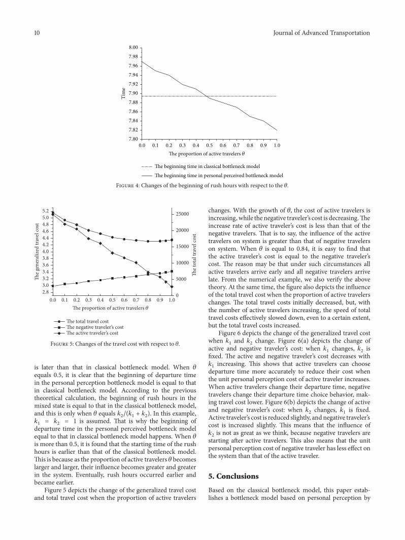

International Journal of
AerospaceEngineeringHindawiwwwhindawicom Volume 2018
RoboticsJournal of
Hindawiwwwhindawicom Volume 2018
Hindawiwwwhindawicom Volume 2018
Active and Passive Electronic Components
VLSI Design
Hindawiwwwhindawicom Volume 2018
Hindawiwwwhindawicom Volume 2018
Shock and Vibration
Hindawiwwwhindawicom Volume 2018
Civil EngineeringAdvances in
Acoustics and VibrationAdvances in
Hindawiwwwhindawicom Volume 2018
Hindawiwwwhindawicom Volume 2018
Electrical and Computer Engineering
Journal of
Advances inOptoElectronics
Hindawiwwwhindawicom
Volume 2018
Hindawi Publishing Corporation httpwwwhindawicom Volume 2013Hindawiwwwhindawicom
The Scientific World Journal
Volume 2018
Control Scienceand Engineering
Journal of
Hindawiwwwhindawicom Volume 2018
Hindawiwwwhindawicom
Journal ofEngineeringVolume 2018
SensorsJournal of
Hindawiwwwhindawicom Volume 2018
International Journal of
RotatingMachinery
Hindawiwwwhindawicom Volume 2018
Modelling ampSimulationin EngineeringHindawiwwwhindawicom Volume 2018
Hindawiwwwhindawicom Volume 2018
Chemical EngineeringInternational Journal of Antennas and
Propagation
International Journal of
Hindawiwwwhindawicom Volume 2018
Hindawiwwwhindawicom Volume 2018
Navigation and Observation
International Journal of
Hindawi
wwwhindawicom Volume 2018
Advances in
Multimedia
Submit your manuscripts atwwwhindawicom