Modeling the temperature effect on the specific growth

HAL Id: hal-01576871https://hal.inria.fr/hal-01576871

Submitted on 24 Aug 2017

HAL is a multi-disciplinary open accessarchive for the deposit and dissemination of sci-entific research documents, whether they are pub-lished or not. The documents may come fromteaching and research institutions in France orabroad, or from public or private research centers.

L’archive ouverte pluridisciplinaire HAL, estdestinée au dépôt et à la diffusion de documentsscientifiques de niveau recherche, publiés ou non,émanant des établissements d’enseignement et derecherche français ou étrangers, des laboratoirespublics ou privés.

Modeling the temperature effect on the specific growthrate of phytoplankton: a review

Ghjuvan Grimaud, Francis Mairet, Antoine Sciandra, Olivier Bernard

To cite this version:Ghjuvan Grimaud, Francis Mairet, Antoine Sciandra, Olivier Bernard. Modeling the temperatureeffect on the specific growth rate of phytoplankton: a review. Reviews in Environmental Science andBio/technology, Springer Verlag, 2017. �hal-01576871�

https://hal.inria.fr/hal-01576871

https://hal.archives-ouvertes.fr

Reviews in Environmental Science and Bio/Technology manuscript No.(will be inserted by the editor)

Modeling the temperature effect on the specific growth rate ofphytoplankton: a review

Ghjuvan Micaelu Grimaud · Francis Mairet ·Antoine Sciandra · Olivier Bernard

Received: date / Accepted: date

Abstract Phytoplankton are key components of ecosystems. Their growth is deeply influencedby temperature. In a context of global change, it is important to precisely estimate the impactof temperature on these organisms at different spatial and temporal scales. Here, we review theexisting deterministic models used to represent the effect of temperature on microbial growth thatcan be applied to phytoplankton. We first describe and provide a brief mathematical analysis ofthe models used in constant conditions to reproduce the thermal growth curve. We present themechanistic assumptions concerning the effect of temperature on the cell growth and mortality,and discuss their limits. The coupling effect of temperature and other environmental factors suchas light are then shown. Finally, we introduce the models taking into account the acclimationneeded to thrive with temperature variations. The need for new thermal models, coupled withexperimental validation, is argued.

Keywords Temperature growth models, thermal growth curve, protein thermal stability,phytoplankton, microalgae, cyanobacteria

1 Introduction

Recent estimations predict a global temperature increase of 1◦C to 5◦C by the year 2100 (Rogelj1

et al, 2012). In this context, the microbial communities, either terrestrial or aquatic, are expected2

to be deeply impacted (Frey et al, 2013; Vezzulli et al, 2012; Thomas et al, 2012). Unicellular3

organisms are ectotherms and cannot regulate their temperature. They are thus particularly sensi-4

tive to temperature, which controls cellular metabolism by affecting enzymatic activity (Privalov,5

1979; Kingsolver, 2009) and stability (Privalov, 1979; Danson et al, 1996; Eijsink et al, 2005).6

Microorganisms play a key ecological role since they are involved in most of the biogeochemical7

fluxes (Paul, 2014; Fuhrman et al, 2015). Especially, the autotrophic unicellular organisms (i.e.8

phytoplankton) are the basis of trophic chains in the majority of ecological systems (Field et al,9

1998). Modeling the effect of temperature on phytoplankton physiology and cellular metabolism is10

thus crucial for better predicting ecosystems evolution in a changing environment.11

In balanced growth conditions, the net growth rate of every microorganism as a function of12

temperature is an asymmetric curve (see fig. 1) called the thermal growth curve or the thermal13

reaction norm (Kingsolver, 2009). The cardinal temperatures corresponding to the boundaries of14

thermal tolerance are defined as the minimal (Tmin) and maximal (Tmax) temperatures for growth.15

The temperature for which growth is maximal is called the optimal temperature (Topt). The growth16

rate obtained at Topt is the maximal growth rate µopt, whenever all the other factors affecting17

growth are non-limiting. The thermal range on which a given species can thrive is the thermal18

Ghjuvan Micaelu Grimaud . Francis Mairet . Olivier BernardBIOCORE-INRIA, BP93, 06902 Sophia-Antipolis Cedex, France. E-mail: [email protected]

Antoine SciandraUPMC Univ Paris 06, UMR 7093, LOV, Observatoire oceanologique, F-06234, CNRS, UMR 7093, LOV, Observatoireoceanologique, F-06234, Villefranche/mer, France.

2 Ghjuvan Micaelu Grimaud et al.

50 µm

Asterionella formosa

Temperature (°C)

Gro

wth

rat

e (d

ay-1)

µopt

Topt TmaxTmin

Fig. 1 Thermal growth curve of the microalgae species Astrionella formosa (redrawn from Bernard and Remond(2012)).

niche width (i.e. Tmax−Tmin). The asymmetry of the growth curve results from differential effects19

on physiology at low (under Topt) and high (above Topt) temperatures. At low temperatures the20

rate of every enzymatic biochemical reactions are affected. At high temperatures, structure and21

stability of some cellular components, such as key enzymes or membrane compounds (mainly lipids22

or proteins) are denatured. The consequences on cell metabolism and integrity leads to an increase23

in mortality (Serra-Maia et al, 2016). These deleterious effects depend on the time spent at high24

temperature, while the ‘thermal dose’ represent the temperature damages (Holcomb et al, 1999).25

The combined effects on metabolism, cell regulation mechanisms and cell integrity give the thermal26

growth curve (Corkrey et al, 2014; Ghosh et al, 2016). While most of these underlying mechanisms27

have not been fully elucidated, several authors have proposed macroscopic models to represent this28

thermal growth curve. These simple models account for a minimum number of variables and do29

not provide a detailed mechanistic description of the involved biochemical underlying phenomena.30

The aim of this study is to summarize the existing deterministic temperature growth models31

that can be used for phytoplankton, and to clarify the assumptions on the considered physiological32

processes. Firstly, models in non-limited and balanced growth conditions (i.e. when all the cell33

variables grow at the same constant rate over time) are described. The key hypotheses are explored34

through the review of growth models as well as the representation of the effect of temperature on35

cell mortality. Secondly, the coupling effect of temperature and other environmental factors such as36

light is addressed. Thirdly, a guideline is proposed to choose a model depending on the modelling37

purposes. Then, we present models taking into account temperature variations. The challenges to38

design a new generation of thermal models are finally discussed.39

Mod

el

Typ

e#

Para

met

ers

Valid

ati

on

(data

sets

)C

ard

inal

tem

per

atu

res

Mort

ali

tyE

mp

iric

al

mod

els

Squ

are

-root

E4

29,

bact

eria

(Ratk

ow

ksy

etal,

1983)

Tmin

an

dTmax

are

exp

lici

tN

oTopt

isfo

un

dby

nu

mer

ical

op

tim

izati

on

CT

MI

E4

47,

bact

eria

&yea

st(R

oss

oet

al,

1993)

Exp

lici

tN

oB

lan

chard

E4

2,

ben

thic

phyto

pla

nkto

n(B

lan

chard

etal,

1996)

Topt

an

dTmax

are

exp

lici

tN

oTmin

isn

ot

defi

ned

Ber

nard

&R

emon

dE

415,

phyto

pla

nkto

n(B

ern

ard

an

dR

emon

d,

2012)

Exp

lici

tN

o

Ep

ple

y-N

orb

erg

SE

45,

phyto

pla

nkto

n(N

orb

erg,

2004)

Topt

=bz−

1+√ (w

/2)2b2

+1

bN

o

ab

s(Tmax−Tmin

)=w

Sem

i-em

pir

ical

mod

els

Arr

hen

ius

equ

ati

on

SE

2-

Not

defi

ned

No

Gen

eral

mech

an

isti

cm

od

els

Mast

erre

act

ion

M4

1,

norm

alize

d,

bact

eria

(Joh

nso

nan

dL

ewin

,1946)

Topt

=∆H‡ /R

ln

( −∆H‡ e∆S−∆He∆

S

∆H

)Y

es

(for

eq.

19)

an

dth

enyea

st(V

an

Ud

en,

1985)

Tmin

an

dTmax

are

not

defi

ned

(im

plici

t)

Hin

shel

wood

M4

No

Topt

=E

1−E

2

Rln

( A 1E

1

A2E

2

)Y

es

Tmax

=E

1−E

2

Rln

( A 1 A2

)(e

xp

lici

t)

Tmin

=Topt

(−E

1/γ

Topt−E

2/γ

)w

ithγ

=R

ln(A

2/A

1ε(E

2−E

1)/E

1)

DE

Bth

eory

M6

No

Tmin

an

dTmax

are

not

defi

ned

Yes

Topt

isfo

un

dnu

mer

ically

(im

plici

t)

Prote

in-s

tab

ilit

yb

ase

dm

od

els

Mod

ified

Mast

erre

act

ion

M4

230,

norm

ali

zed

,all

mic

roorg

an

ism

s(C

ork

rey

etal,

2014)

Topt

=∆CpT0

+∆H

∆Cp

+R

Yes

Tmin

an

dTmax

are

not

defi

ned

(im

plici

t)P

rote

om

eb

ase

dM

212,

norm

alize

d,

bact

eria

(Dil

let

al,

2011)

Tmin

an

dTmax

are

not

defi

ned

Yes

Topt

isfo

un

dnu

mer

ically

(im

plici

t)H

eat

cap

aci

tyb

ase

dM

412,

soil

pro

cess

es(S

chip

per

etal,

2014)

Tmin

,Topt,Tmax

are

fou

nd

nu

mer

ically

No

Tab

le1

Synth

esis

of

the

main

mod

els

for

gro

wth

rate

as

afu

nct

ion

of

tem

per

atu

re(s

eeals

ose

ctio

n3.1

).E

,em

pir

ical

mod

els.

M,

mec

han

isti

cm

od

els.

SE

,se

mi-

emp

iric

al

mod

els.

‘Valid

ati

on

’co

rres

pon

ds

toth

eori

gin

al

data

sets

use

dto

dev

elop

an

dvalid

ate

the

mod

els.


0 10 20 30

0

0.2

0.4

0.6

0.8

1

Ratkowsky

0 10 20 30

0

0.2

0.4

0.6

0.8

1

CTMI

0 10 20 30

0

0.2

0.4

0.6

0.8

1

Blanchard

0 10 20 30

0

0.2

0.4

0.6

0.8

1

MRM

0 10 20 30

0

0.2

0.4

0.6

0.8

1

Hinshelwood

0 10 20 30

0

0.2

0.4

0.6

0.8

1

MMRM

0 10 20 30

0

0.2

0.4

0.6

0.8

1

Proteome

0 10 20 30

0

0.2

0.4

0.6

0.8

1

Heat Capacity

0 10 20 30

0

0.2

0.4

0.6

0.8

1

Eppley−Norberg

0 10 20 30

0

0.2

0.4

0.6

0.8

1

DEB

Square-root CTMI Blanchard MRM* Hinshelwood

DEB MMRM* Proteome* Heat-capacity*Eppley-Norberg

Temperature (°C)

Nor

mal

ized

µ(T

)

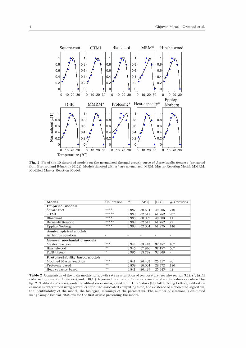
Fig. 2 Fit of the 10 described models on the normalized thermal growth curve of Asterionella formosa (extractedfrom Bernard and Remond (2012)). Models denoted with a * are normalized. MRM, Master Reaction Model, MMRM,Modified Master Reaction Model.

Model Calibration r2 |AIC| |BIC| # CitationsEmpirical modelsSquare-root **** 0.987 50.694 49.906 710CTMI ***** 0.989 52.541 51.752 267Blanchard **** 0.988 50.092 49.303 111Bernard&Remond ***** 0.989 52.541 51.752 77Eppley-Norberg **** 0.988 52.064 51.275 146

Semi-empirical modelsArrhenius equation - - - - -

General mechanistic modelsMaster reaction *** 0.944 33.443 32.457 107Hinshelwood ** 0.945 37.946 37.157 507DEB theory * 0.985 33.748 32.368 -

Protein-stability based modelsModified Master reaction *** 0.841 26.403 25.417 20Proteome based ** 0.839 30.064 29.472 126Heat capacity based ** 0.841 26.429 25.443 42

Table 2 Comparison of the main models for growth rate as a function of temperature (see also section 3.1). r2, |AIC|(Akaike Information Criterion) and |BIC| (Bayesian Information Criterion) are the absolute values calculated forfig. 2. ‘Calibration’ corresponds to calibration easiness, rated from 1 to 5 stars (the latter being better); calibrationeasiness is determined using several criteria: the associated computing time, the existence of a dedicated algorithm,the identifiability of the model, the biological meanings of the parameters. The number of citations is estimatedusing Google Scholar citations for the first article presenting the model.

Modeling the temperature effect on the specific growth rate of phytoplankton: a review 5

2 Modeling the specific growth rate of unicellular organisms as a function oftemperature: the thermal growth curve

In this section, we detail the existing models dedicated to the effect of temperature on the specific40

growth rate of microorganisms in non-limiting conditions (see table 1 and 2 for a summary). As41

discussed latter on, the specific growth rate concept (i.e. biomass increase per unit of time per unit42

of biomass) is highly dependent on the biomass descriptor.43

2.1 Experimental and methodological clarifications

The specific growth rate is defined, in batch acclimated cultures, as the specific biomass growth44

rate during the exponential phase:45

µ(T ) =1

X

dX

dt=

ln(2)

g(T )(1)

where T is a fixed temperature, X is the biomass concentration and g(T ) is the generation time46

(i.e the time it takes to double the population size). The organisms are assumed to be in balanced47

growth conditions as defined by Campbell (1957) (i.e. every extensive property of the growing48

system increases by the same factor over a time interval), for a period long enough so that the49

acclimation processes have reached their steady state. µ(T ) is commonly called the thermal growth50

curve or the thermal reaction norm (Kingsolver, 2009).51

It is important to note that in practice the thermal growth curve depends on different factors,52

especially the way biomass is measured. Firstly, different biomass descriptors are commonly used,53

such as cell counts, particulate organic carbon concentration (POC), total cell biovolume or optical54

density. The dynamics of some descriptors is likely to be affected differentially by temperature55

than, for example, the dynamics of cell concentration. In phytoplankton, the chlorophyll content56

is a function of temperature (Geider, 1987), and thus the evolution of optical density results both57

from the growth process and from the shift in the cellular optical properties. An ideal biomass58

estimate should be proportional to the carbon mass with a temperature-independent constant.59

The difficulty to compare observations from different studies is inherent to heterogeneity in the60

measured descriptors.61

Secondly, the experimental protocols are most of the time unclear on the acclimation period62

preceding the growth measurement. Acclimation time can vary from one day to several weeks63

(Boyd et al, 2013; Corkrey et al, 2014). In some cases, biomass evolution is probably affected64

by acclimation to the new temperature. For example, some experimental protocols proceed by65

gradually increasing temperature and measuring the growth rate. The main advantage is that they66

provides a rapid evaluation of the temperature response, but the recorded response reflects a mix67

between a transient acclimation phase and the effect of temperature on the cell metabolism. The68

possible bias is however even stronger when the descriptor used is related to carbon content with69

a temperature-dependent constant. For example, a too short period of acclimation results in a still70

evolving biomass to chlorophyll a ratio. Therefore, if the growth rate is estimated using chlorophyll71

a concentration (or turbidity) the computed growth rate will be biased.72

The growth rate estimated from oxygen production must also be considered with care. The light73

phase of photosynthesis is mainly a photochemical process and is hardly affected by temperature at74

temperatures below Topt. Carbon dioxide fixation in the Calvin cycle is an enzymatic process which75

is highly temperature dependant. Estimating growth rate from oxygen production will thus mask76

most of the temperature impact if an acclimation period has not been considered. The experimental77

acclimation period at a given temperature is of major importance for the consistency of the thermal78

growth curve.79

For all these reasons, Boyd et al (2013) have developed a protocol to construct the thermal80

growth curve for phytoplankton and optimize the comparability of different thermal growth curves81

between different experiments and different species. This protocol specifies that:82

1. the population must be acclimated to the experimental temperature for at least 4 generations83

(we recommend even 7 generations),84

2. the population must be kept at an exponential growth phase using semi-continuous cultures,85


3. multiple biomass descriptors must be used and compared to obtain growth rates (cell counts,86

chlorophyll a fluorescence, etc.); we recommend to consider carbon or dry weight for biomass,87

4. a minimum of 6 experimental growth rates at 6 different temperatures must be obtained,88

5. the cultures must be carried out with three replicates,89

6. all the other parameters must be kept constant, if possible at optimal levels,90

7. the experiments with temperatures at which the cells do not grow or grow very slowly must be91

repeated several times,92

8. several strains of the same species should be compared.93

2.2 Empirical approach to model the thermal growth curve

Various empirical models (i.e. not developed from biological assumptions) have been proposed94

since the 1960’s to represent the thermal growth curve, but only three are still commonly used.95

Historically, these models have mostly been developed for food-processing industry and medical96

applications.97

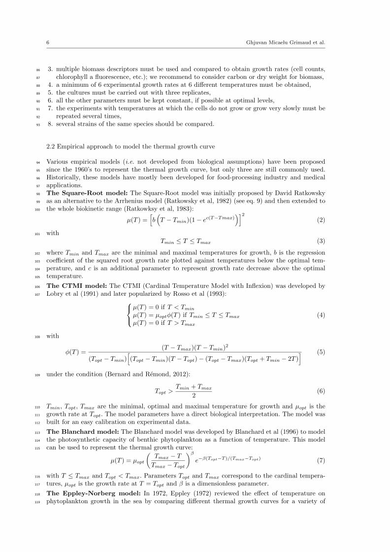
The Square-Root model: The Square-Root model was initially proposed by David Ratkowsky98

as an alternative to the Arrhenius model (Ratkowsky et al, 1982) (see eq. 9) and then extended to99

the whole biokinetic range (Ratkowksy et al, 1983):100

µ(T ) =[b(T − Tmin)(1− ec(T−Tmax)

)]2(2)

with101

Tmin ≤ T ≤ Tmax (3)

where Tmin and Tmax are the minimal and maximal temperatures for growth, b is the regression102

coefficient of the squared root growth rate plotted against temperatures below the optimal tem-103

perature, and c is an additional parameter to represent growth rate decrease above the optimal104

temperature.105

The CTMI model: The CTMI (Cardinal Temperature Model with Inflexion) was developed by106

Lobry et al (1991) and later popularized by Rosso et al (1993):107 µ(T ) = 0 if T < Tminµ(T ) = µoptφ(T ) if Tmin ≤ T ≤ Tmaxµ(T ) = 0 if T > Tmax

(4)

with108

φ(T ) =(T − Tmax)(T − Tmin)2

(Topt − Tmin)[(Topt − Tmin)(T − Topt)− (Topt − Tmax)(Topt + Tmin − 2T )

] (5)

under the condition (Bernard and Remond, 2012):109

Topt >Tmin + Tmax

2(6)

Tmin, Topt, Tmax are the minimal, optimal and maximal temperature for growth and µopt is the110

growth rate at Topt. The model parameters have a direct biological interpretation. The model was111

built for an easy calibration on experimental data.112

The Blanchard model: The Blanchard model was developed by Blanchard et al (1996) to model113

the photosynthetic capacity of benthic phytoplankton as a function of temperature. This model114

can be used to represent the thermal growth curve:115

µ(T ) = µopt

(Tmax − TTmax − Topt

)βe−β(Topt−T )/(Tmax−Topt) (7)

with T ≤ Tmax and Topt < Tmax. Parameters Topt and Tmax correspond to the cardinal tempera-116

tures, µopt is the growth rate at T = Topt and β is a dimensionless parameter.117

The Eppley-Norberg model: In 1972, Eppley (1972) reviewed the effect of temperature on118

phytoplankton growth in the sea by comparing different thermal growth curves for a variety of119


w

z

Temperature (°C)

Gro

wth

rat

e (d

oubl

ing

per

day-1

)

Fig. 3 A, Eppley envelope function with the original data points. B, 5 data sets for eukaryotic phytoplanktonspecies. C, Eppley-Norberg plot for the 5 species (redrawn from Norberg (2004)).

phytoplankton species in non-limiting conditions (nearly 200 data points). Eppley (1972) deter-120

mined that the maximal growth rate µopt for each species is constrained by a virtual envelope along121

the optimal temperature trait Topt, the so-called ‘Eppley curve’ (see fig. 3). Eppley (1972) stated122

that for any phytoplankton species growing under 40◦C, ‘hotter is faster’.123

Using Eppley’s hypothesis, Norberg (2004) developed a temperature-growth model, the ‘Eppley-124

Norberg’ model:125

µ(T ) =

[1−

(T − zw

)2]aebT (8)

where w is the thermal niche width, z is the temperature at which the growth rate is equal to126

the Eppley function and is a proxy of Topt, a and b are parameters of the Eppley function. The127

Eppley-Norberg model is widely used by the scientific community working on phytoplankton (e.g.128

see the recent paper of Taucher et al (2015)).129

2.3 Empirical model comparison130

A comparison between the Square-Root model and the CTMI was made by Rosso et al (1993) and131

more recently by Valik et al (2013). According to these studies, the two models fit equally well132

the data. Both models are validated by Valik et al (2013) using an F-test. However, the b and c133

parameters of the Square-root model are correlated, whereas the CTMI parameters are not, which134

allows easier parameter identification.135

A more extensive comparison between the set of empirical models is presented on Figure 2136

for Asterionella formosa. It turns out that most of them can successfully describe this data set,137

but the fit is almost perfect for the CTMI and the Square-Root model. The CTMI proves useful138

for cardinal temperatures identification since all these parameters have a biological meaning. A139

guideline for choosing the most appropriate model is proposed in the discussion section.140

2.4 Semi-empirical approach141

Semi-empirical models use a combination of biological mechanisms and empirical formulations. The142

very first temperature model, the Arrhenius equation, was developed in this way.143


The Arrhenius equation: In the beginning of the 20th century, the work of Jacobius Van’t-144

Hoff and Svante Arrhenius on the effect of temperature on chemical reactions (Arrhenius, 1889)145

was introduced in biology by Charles Snyder (Snyder, 1906), setting that temperature has an146

exponential influence on biological reactions and then on cellular growth according to the following147

equation called ‘the Arrhenius law’:148

k(T ) = Ae−E/(RT ) (9)

where k(T ) is the rate of reaction, R is the gas constant, A is called the ‘collision factor’ or the149

pre-exponential part and E is the activation energy, determined empirically. The Arrhenius equa-150

tion is semi-empirical, partially based on thermodynamical considerations; it can be interpreted151

as the number of collisions per unit of time multiplied by the probability that a collision results152

in a reaction. The Arrhenius equation is widely used to describe the temperature effect on differ-153

ent biological processes, from enzyme catalysis to community activity (e.g. see Frauenfelder et al154

(1991), Lloyd and Taylor (1994), Gillooly et al (2001)). However, it is only valid on a small range155

of temperature, excluding high temperatures inhibiting growth (Slator, 1916). Arrhenius model156

parameters are easy to estimate using an Arrhenius plot, by expressing ln(µ(T )) as a function of157

1/T , which gives a linear relationship; parameters can thus be obtained with a linear regression.158

The Arrhenius model allows good representations of growth rates at low temperatures, but some159

Arrhenius plot does not give straight lines, indicating for example that E can vary with T . More-160

over, the Arrhenius model cannot represent the decreasing part of the thermal growth curve, e.g.161

when temperature causes cell death. Arrhenius equation can be conveniently reformulated as:162

k(T ) = kreTA/Tr−TA/T (10)

where Tr is a reference temperature, TA is the Arrhenius temperature (i.e. slope of the straight163

line of the Arrhenius plot) and kr is the reaction rate at Tr.164

2.5 Mechanistic approach165

The empirical models are convenient to identify the main characteristics of the thermal growth166

curve. However, the mechanistic approach aims to represent the thermal growth curve as a result of167

the inherent physiological processes. These models are mostly based on the Arrhenius formulation,168

but also on the Eyring equation. In addition to their explanatory role, because their parameters169

have thermodynamical meanings, it is possible to extract thermodynamical informations from the170

thermal growth curve only.171

2.5.1 General models based on the Arrhenius and Eyring formulations172

The Eyring equation and the Transition-State theory: this theory stipulates that, during a173

chemical reaction, there exists an intermediate form between the reactants and the products (e.g.174

the native and denatured protein and enzyme) which is in rapid equilibrium with the reactants175

(Eyring, 1935):176

Pfk1k2TS

kd→ Pu (11)

where, in this example, Pf and Pu are the fraction of native and denatured proteins, respectively,177

and TS is the transition state. The Eyring equation, roughly similar to the Arrhenius law, was178

nonetheless based on these pure mechanistic considerations and reads (Eyring, 1935):179

k(T ) =KBT

he∆S

‡/Re−∆H‡/(RT ) (12)

where KB is the Boltzmann constant, h is the Planck’s constant. The parameters ∆S‡ and ∆H‡180

correspond to the entropy and enthalpy of activation for the transition state.181

The master reaction model: In 1946, Johnson and Lewin noticed that cultures of Escherichia182

coli exposed to 45◦C during a long time ceased to grow, but grew exponentially again when replaced183

at 37◦C. The longer the cultures were exposed to the high temperature, the lower was the growth184

rate at 37◦C. However, there was no sign of viability loss. They concluded that cells endured185

reversible damage, particularly protein denaturation. They considered a simple case where a single186

reaction controlled by one master enzyme En limits growth (with no substrate limitation):187


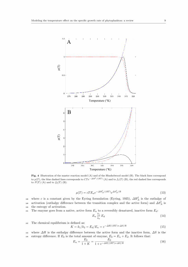
Temperature (°K)

Temperature (°K)

A

B

µ(T

)µ

(T)

Fig. 4 Illustration of the master reaction model (A) and of the Hinshelwood model (B). The black lines correspond

to µ(T ), the blue dashed lines corresponds to CTe−∆H‡/(RT ) (A) and to f1(T ) (B), the red dashed line corresponds

to P (T ) (A) and to f2(T ) (B).

µ(T ) = cTEne−∆H‡

A/(RT )e∆S‡A/R (13)

where c is a constant given by the Eyring formulation (Eyring, 1935), ∆H‡A is the enthalpy of188

activation (enthalpy difference between the transition complex and the active form) and ∆S‡A is189

the entropy of activation.190

The enzyme goes from a native, active form En to a reversibly denatured, inactive form Ed:191

Enk1k2Ed (14)

The chemical equilibrium is defined as:192

K = k1/k2 = Ed/En = e−∆H/(RT )+∆S/R (15)

where ∆H is the enthalpy difference between the active form and the inactive form, ∆S is the193

entropy difference. If E0 is the total amount of enzyme, E0 = En + Ed. It follows that:194

En =E0

1 +K=

E0

1 + e−∆H/(RT )+∆S/R(16)


Then, by posing C = ce∆S‡A/RE0 and replacing En by eq. 16 in eq. 13, Johnson and Lewin obtained195

the master reaction model (see fig. 4 A):196

µ(T ) = CTe−∆H‡A/(RT ) · 1

1 + e−∆G(T )/(RT )︸︷︷︸P (T )

(17)

where P (T ) is the probability that the enzyme is in its native state and ∆G(T ) is the Gibbs free197

energy change:198

∆G(T ) = ∆H − T∆S (18)

However, the master reaction model assumes that ∆G is temperature independent. An other version199

of eq.17 exists, where the exponential part does not follow an Eyring formulation but rather an200

Arrhenius one, which is relevant in the case of reactions with high activation energy like protein201

denaturation (Bischof and He, 2005):202

µ(T ) = Ce−∆H‡A/(RT ) · 1

1 + e−∆G(T )/(RT )(19)

It is worth noting that this equation here simplifies the calculation of the cardinal temperature203

Topt and is supposed to have little influence on the model fit and behavior (see table 1 and 2).204

The Hinshelwood model: In 1945, Sir Norman Hinshelwood proposed a rather simple model in205

which the temperature-dependent growth rate is just the difference between a synthesis rate f1(T )206

and a degenerative rate f2(T ) (Hinshelwood, 1945) (see fig. 4 B):207

µ(T ) =

f1(T )︷︸︸︷A1e

−E1/(RT )−A2e−E2/(RT )︸︷︷︸f2(T )

(20)

where A1 and A2 are related to entropy and E1 and E2 are related to enthalpy. Hinshelwood208

believed that the function f2(T ), which causes the ‘catastrophic decline to zero’(Hinshelwood,209

1945), represents protein denaturation. He argued that the model only works if E2 is higher than E1,210

because the degenerative process represented by f2(T ) must be sudden. Since protein denaturation211

possesses a high activation energy, it is a good candidate for driving the process. Moreover, A2212

(corresponding to entropy) also has to be quite high. Thus, the ‘activated state must be highly213

disordered compared with the initial state’ which ‘results in an easy transition to the activated state214

in spite of the large amount of energy which has to be taken up to reach it ’(Hinshelwood, 1945).215

Precisely, protein denaturation leads from a highly ordered state to an higly disordered state and216

is therefore associated with a large entropy increase. From the Hinshelwood model, after some217

mathematical manipulations, it is possible to express Tmin, Topt, Tmax (see table 1).218

The DEB theory approach: In the Dynamics Budget Theory, the effect of temperature on219

population growth is taken into account using a modified Master Reaction model (Kooijman,220

2010), where all the temperature-dependent functions are Arrhenius modified equations:221

µ(T ) =k1e

TA/T1−TA/T

1 + eTAL/T−TAL/TL + eTAH/TH−TAH/T︸︷︷︸fD

(21)

where TL and TH are related to cold and hot denaturation (lower and upper boundaries), TAL and222

TAH are the Arrhenius temperatures (i.e. the slope of the straight line of the Arrhenius plot at223

low and high temperatures respectively, see eq. 10). The ratio f−1D corresponds to the fraction of224

enzyme in its native state. This model therefore also accounts for cold denaturation, contrary to225

the Master Reaction model.226

2.5.2 The protein thermal stability hypothesis227

In addition to the temperature-dependent enzyme activity, protein thermal stability plays a key role228

in the microbial thermal growth curve (Johnson and Lewin, 1946; Rosenberg et al, 1971; Zeldovich229

et al, 2007; Pena et al, 2010). If temperature increases, certain proteins become first inactive and230

then denatured. Especially, at high temperatures (T > Topt), this phenomenon occurs for many231

proteins and causes a growth rate decrease. In line with the master reaction model, some models232


C

Nor

mal

ized

µ(T

)

Temperature (°K)

Fig. 5 The modified master reaction model plot for a microbial species (black line) with activation function (bluedashed line) and protein denaturation probability P (T ) (red dashed line).

include additional assumptions about protein thermal stability and its consequences on growth,233

assuming that proteins are the key factors controlling thermal growth curves.234

The modified master reaction model: The master reaction model assumes that ∆G, the235

Gibbs free energy difference between the native and denatured protein, is temperature independent.236

Based on Murphy et al (1990) work, Ross (1993) and then Ratkowsky et al (2005) remarked that237

∆G should vary with T in eq. 17 following eq. 18. Moreover, Murphy et al (1990) showed that238

globular proteins (including enzymes) share common thermodynamic properties. For any protein,239

the denaturation enthalpy change (∆H) and the denaturation entropy change (∆S), normalized to240

the number of amino-acids residues of this protein, both converge to a fixed value ∆H∗ and ∆S∗241

at T ∗H and T ∗S respectively (Privalov, 1979). The reason for such a temperature convergence is still242

unclear. Nonetheless, it has been shown that, at T ∗H and T ∗S , the hydrophobic contribution to ∆H243

and ∆S approaches zero (Robertson and Murphy, 1997). Using the heat capacity thermodynamic244

parameter Cp, Murphy et al (1990) stated that ∆H and ∆S can be expressed as a function of the245

heat capacity change ∆Cp:246

∆H = ∆H∗ +∆Cp(T − T ∗H) (22)

∆S = ∆S∗ +∆Cpln(T/T ∗S) (23)

where ∆H∗ is the enthalpy change per mol of amino-acid residue of the enzyme at T ∗H , ∆S∗ is247

the entropy change per mol of amino-acid residue of the enzyme at T ∗S , ∆Cp is the heat capacity248

difference between the native and denatured protein, T ∗H is the temperature at which the contri-249

bution of ∆Cp to enthalpy is zero and T ∗S is the temperature at which the contribution of ∆Cp250

to entropy is zero. The heat capacity change ∆Cp is constant for a given protein (Privalov and251

Khechinashvili, 1974). Using eq. 22 and eq. 23, the Gibbs free energy of protein denaturation (i.e.252

the protein thermal stability) is (fig. 5):253

∆G(T ) = n[∆H∗ − T∆S∗ +

∆Ghydro︷︸︸︷∆Cp[(T − T ∗H)− T ln(T/T ∗S)]

](24)

where n is the number of amino-acid residues in the master enzyme and ∆Ghydro is the hydrophobic254

contribution to the free energy change. Eq. 24 describes protein thermal stability in terms of255

hydrophobic contribution of apolar compounds.256

Ross (1993) and Ratkowsky et al (2005) proposed to replace ∆G by eq. 24 in eq. 17 (forming the257

modified master reaction model). Because T ∗H , T ∗S and ∆S∗ are considered as universal constant258

for globular proteins (Murphy and Gill, 1991), the modified master reaction model has 5 tunable259


Num

ber

of p

rote

ins

P(Δ

G)

0 10 20 30 40ΔG(RT)

0

100

200

300

400 0.1

0.025

0.075

0.05

0

Fig. 6 Gibbs free energy distribution of Escherichia coli proteome at 37◦C (adapted from Ghosh and Dill (2010)).

parameters (fig. 5). As a validation, Ratkowsky et al (2005) fitted the model on 35 bacterial strains260

normalized data sets obtained in non-limiting conditions. Their main conclusion points towards the261

crucial role played by a single master enzyme whose thermal sensitivity is driven by hydrophobic262

interactions.263

Corkrey et al (2014) extended the modified master reaction model to unicellular and multi-264

cellular eukaryotes. They considered ∆H∗ as a universal constant as well, reducing the model265

parameters to 4. They fitted the model on 230 strains normalized data sets covering a range of266

124◦C. Their principal conclusion states that the model is able to find coherent protein ther-267

modynamics parameters with only net growth rates data (i.e. growth rate versus temperature).268

Hyperthermophiles proteins seem to be more widely robust. Moreover, they found several links269

between thermodynamic parameters, for example between Topt and ∆Cp (enzyme stability), and270

between Topt and ∆H‡ (enzyme activity). However, they did not provide further explanations.271

They finally speculate on the nature of the single limiting reaction. They assume that if a single272

reaction (and not several) is rate limiting, then it should be linked to the protein unfolding and273

re-folding process. They particularly focus on the role of chaperones proteins responsible for de274

novo folding.275

The proteome-scale approach: Zeldovich et al (2007) proposed that the whole proteome276

plays a role in microbial thermal sensitivity. Resuming this idea, Chen and Shakhnovich (2010)277

considered that each important protein i has its own Gibbs free energy of denaturation ∆Gi. The278

growth rate of a microbe becomes dependent of the stability of each protein, and the thermal279

denaturation of several proteins causes a bottleneck effect on growth:280

µ(T ) = CTe−∆H‡/(RT ) · 1

Np∏i

1 + e−∆Gi(T )/(RT )

(25)

where Np is the number of proteins. According to Zeldovich et al (2007), the proteome can be281

described in protein stability distribution thanks to a dedicated probability function of the Gibbs282

free energy, P (∆G) (see fig.6). By taking the natural logarithm of eq. 25, Chen and Shakhnovich283

(2010) expressed the growth rate as:284

ln(µ(T )) = ln(CT )−∆H‡/(RT )−Np∑i=1

ln(

1 + e−∆Gi/(RT ))

(26)

that is, by integrating the resulting equation over the whole P (∆G) distribution range and by285

averaging over the proteome:286


ln(µ(T )) ' ln(CT )−∆H‡/(RT )−Np∫ L

0

ln(

1 + e−∆G/(RT ))P (∆G) d∆G (27)

where L is the maximum value of ∆G (for example L = 40 in fig. 6). Np can be reduced to the287

number of the only important proteins. According to Sawle and Ghosh (2011) and Ghosh and Dill288

(2010), ∆G can be expressed as a function of ∆H, ∆S and ∆Cp (using eq. 22 and eq. 23), itself289

depending on the protein chain length denoted N :290

∆G = ∆H(N) +∆Cp(N)(T − Th)− T∆S(N)− T∆Cp(N)ln (T/Ts) (28)

with291

∆H(N) = aN + b∆S(N) = cN + d∆Cp(N) = lN +m

(29)

where a, b, c, d, l,m are empirical parameters defined for mesophilic and for thermophilic organisms.292

The distribution of chain length over the proteome P (N) can be known (Zhang, 2000) and is used293

to estimate P (∆G). It can be modelled by a gamma distribution:294

P (N) =Nα−1e−N/θ

Γ (α)θα(30)

where θ and α are the parameters of the gamma distribution corresponding to:295

< N >= αθ< (∆N)2 >= αθ2

(31)

The brackets represent the mean over all the proteins. Γ (α) is the gamma function evaluated at296

α. The model (eq. 27), presented as universal, has thus only two parameters, Np and ∆H‡. It has297

been validated on 12 normalized data sets of prokaryotes.298

The heat capacity hypothesis: Hobbs et al (2013) and Schipper et al (2014) proposed a299

model called the Macromolecular Rate Theory (MMRT) in which the thermal growth curve is300

driven by the heat capacity change of activation ∆C‡p (i.e. the heat capacity difference between301

the ground state and the transition state). More precisely, the growth rate is expressed as:302

µ(T ) =kBhTe∆G

‡(T )/(RT ) (32)

where kB and h are the Boltzmann and Planck’s constants, ∆G‡ is the Gibbs free energy difference303

between the ground state and the transition state of a possible rate-limiting enzyme. Contrary to304

the master reaction model, the MMRT considers that enzymes do not denature easily and are in305

rapid equilibrium with a folded, inactive intermediate (i.e. the transition state). The Gibbs free306

energy difference can be here written as:307

∆G‡(T ) = ∆H‡T0+∆C‡p(T − T0) + T (∆S‡T0

+∆C‡pln(T/T0)) (33)

If ∆C‡p > 0, then the heat capacity difference between the ground state and the transition state308

(i.e. the inactive folded enzyme) itself is sufficient to explain the decrease of growth rate above309

Topt. Schipper et al (2014) validated the MMRT model on microbial soil processes data sets.310

2.6 Mortality induced by temperature311

Warm temperatures increase cell mortality because of protein denaturation and membranes in-312

juries. For phytoplankton, photosystems and electron chain transport are denaturated (Song et al,313

2014), and a transient imbalance between the energy needed and produced must be managed by314

the cell (Ras et al, 2013; Smelt and Brul, 2014; Serra-Maia et al, 2016).315

So far, models explicitly presenting the mortality rate as a function of temperature are rare.316

The Hinshelwood model explicitly integrates a mortality rate with an Arrhenius law (see fig. 7 B).317

This model turned out to efficiently represent mortality together with growth for the chlorophyta318

Chlorella vulgaris (Serra-Maia et al, 2016). Another example is Van Uden (1985) who combined a319

master reaction growth model and an exponential death model for yeast:320


ln(N(t)/N0)

Time (t)

B

Temperature (T)

Growthrateµ(T)

Time (min) Time (min)

ln(N(t))

52.5°C 65°CA

Fig. 7 A, Survival curves at different temperatures for Listeria innocus (redrawn from Corradini and Peleg (2006)).B, Hinshelwood model (black curve) with mortality (red curve) as in Serra-Maia et al (2016).

µ(T ) =Ce−∆H

‡/(RT )

1 + e−∆G/(RT )− kBT

he∆S

‡den/R−∆H

‡den/(RT ) (34)

where ∆S‡den and ∆H‡den are the entropy and enthalpy of activation of cells mortality.321

Outside of the thermal niche width, for temperatures above the species Tmax, the kinetics of322

cell inactivation is called the survival curve (Moats, 1971) (fig. 7 A); from each survival curve, it is323

possible to infer the mortality rate at a given temperature. Different empirical models have been324

developed, especially in food science, to represent these survival curves (Mafart et al, 2002; Smelt325

et al, 2002; Smelt and Brul, 2014).326

3 Choosing the most appropriate model327

In this section, we propose a guideline for choosing the most appropriate model depending on the328

study objectives. We summarize and compare the models performance and their applicability to329

phytoplankton in different modeling scenario, and highlight the most appropriate models.330

The model comparison is based on the analysis of 193 thermal curve responses associated to331

193 different strains, resulting from 130 species (Thomas et al, 2012). This data set includes the332

main phyla of unicellular photosynthetic organisms.333

An illustration of the model performance for 5 strains of the cyanobacterium genus Synechococ-334

cus sp. is plotted on fig. S1 (Pittera et al, 2014).335


3.1 Synthesis of model performance336

Three criteria have been considered to assess a model efficiency. The absolute model performance337

is estimated using r2. To account both for the fit quality and the number of parameters, we338

considered the Akaike Information Criterion (AIC) (Akaike, 1992) and the Bayesian Information339

Criterion (BIC) (Schwarz et al, 1978) (see table 2 and table S1-S3). The best models are, globally,340

the empirical models, and the CTMI and the Eppley-Norberg turn out to obtain the best score341

(see table S2, fig. S2). The Hinshelwood model, in the other way, has the best score among the342

mechanistic models. It is worth noting here that the CTMI assumes that Tmax−Topt ≤ Topt−Tmin,343

which is not the case for the Eppley-Norberg. Thus, for small data sets with few points near Topt,344

the Eppley-Norberg model has a better fit score (see fig. S3).345

To highlight the combination of fit quality and other important characteristics, we defined346

several criterions in table 1. From these criterions, we could derive advantages, limitations and347

rating for each model (table 1). The CTMI, Bernard&Remond and the Hinshelwood model obtain348

the highest score, with the best trade-off between complexity (e.g. few parameters), fit quality,349

calibration easiness and parameters interpretation.350

3.2 Macroscopic modeling without including mortality351

A common scenario when modeling the effect of temperature on phytoplankton is the need of352

representing the net thermal response, without explicitly representing mortality. The response is353

generally focusing on growth rate, but it can also represent a detailed physiological processes. Below354

the optimal temperature, the Arrhenius equation has been widely used, has a good fit, is easy to355

calibrate and its parameters can be interpreted. However, to represent the whole thermal growth356

curve, the CTMI is the best choice because its parameters are directly the cardinal temperatures357

and its calibration is easily possible thanks to a dedicated algorithm. Other similar models (e.g.358

Eppley-Norberg) are also satisfactory. When light is not photoinhibiting, these models can be359

easily combined with the light effect on growth. In particular, the Bernard&Remond model is a360

good trade-off. This latter model has been originally validated on 15 phytoplankton species and361

here on 193 phytoplankton species (table S1-S3) from the main phytoplankton phyla. The CTMI362

is thus expected to be the ideal candidate to represent the effect of temperature on phytoplankton363

communities. The Eppley-Norberg model is also interesting for modeling communities given that364

from its four parameters, two are considered universal and only two are strain-specific.365

3.3 Macroscopic modeling with explicit mortality rate366

As we pointed out, few studies exist to represent the effect of temperature on phytoplankton367

mortality. The only model that explicitly represents mortality is the Hinshelwood model. Adapted368

for phytoplankton (Serra-Maia et al, 2016), this model is thus recommended because its parameters369

can be interpreted, and the fit quality is acceptable; however, its parameters calibration are not370

easy on experimental data with few data points. We thus recommend to use the CTMI to generate371

a patron for the net growth rate. The patron, made of the data points simulated by the CTMI372

model can then be advantageously used to calibrate the Hinshelwood model.373

3.4 Physiological or metabolic modeling374

The proteome model is certainly the best candidate to explain the thermal growth curve, as it375

includes the effect of temperature on the whole proteome and has only two parameters. However,376

it does not fit very well the experimental data for phytoplankton growth rates compared to the377

empirical models. As for the Hinshwelwood model, a patron can be used to artificially increase378

the number of data points. This model could also be adapted to phytoplankton when light is379

photoinhibiting.380


Model Advantages Limitations RatingSquare-root Fit quality No mortality, Topt ***

is not easily definedCTMI Fit quality, No mortality ****

parameters interpretationBlanchard Calibration easiness, fit quality, No mortality ***

application to phytoplankton Tmin is not definedBernard&Remond Calibration easiness, fit quality, No mortality *****

parameters interpretation,application to phytoplankton

Eppley-Norberg Fit quality, No mortality, implicit linkapplication to phytoplankton between Topt and µopt ****

Arrhenius equation Fit quality No representation of the **below Topt decreasing phase above Topt

Master reaction Parameters interpretation Tmin and Tmax **are undefined

Hinshelwood Fit quality, parameters Tmin is not defined ****interpretation, explicit mortality

DEB theory Fit quality High number *of parameters

Modified Master reaction Parameters intepretation Poorness of fit **

Proteome based Parameters intepretation, Poorness of fit ***only 2 parameters

Heat capacity based - Poorness of fit, parameters *interpretation not clear

Table 3 Advantages, limitations and rating of the main models for growth rate as a function of temperature. Ratingis based on criterion from table 1, from 1 to 5 stars (the latter being better).

4 Coupling temperature and other environmental factors381

4.1 Factors influencing the thermal growth curve382

The thermal growth curve is assumed to be obtained in non-limited conditions (Kingsolver, 2009).383

However, some limitations and perturbations usually occur in the environment that may simultane-384

ously involve changes in metabolism. The simplest representation of some multi-factors impact on385

the growth rate is to assume that all the factors are uncoupled. A classical formalism to represent386

the effect of n uncoupled factors is given by the gamma concept (Zwietering et al, 1993; Augustin387

and Carlier, 2000):388

µ = µopt.

n∏k=1

γk (35)

where µopt is the maximal growth rate when all the n environmental factors are optimal, γk389

is a normalized function of the environmental factor k. One of the γk represents the impact of390

temperature.391

In a more accurate approach, the impact of a factor on the cardinal temperatures can be repre-392

sented (or more generally the parameters of the thermal model can be a function of another factor).393

In this case, these environmental factors are coupled to temperature. For example, temperature394

plays a role on oxygen dissolution in water, and the two factors have then a coupled effect on395

microbial growth rates; this coupling is enhanced for unicellular diazotrophic cyanobacteria which396

are particularly sensitive to the oxygen concentration, because oxygen inhibits their diazotrophic397

activity (Brauer et al, 2013).398

For the majority of phytoplankton species, the most important physico-chemicals factors are399

light and nutrients (mainly N and P) (Falkowski and Raven, 2013).400

4.2 The interplay between light and temperature in phytoplankton401

Phytoplankton perform oxygenic photosynthesis to harvest light. Photosynthesis metabolism is402

composed of a dark phase and a light phase, with different thermal sensitivities. The dark phase403


involves the Rubisco enzyme responsible for CO2 fixation in the Calvin cycle. In the light phase, at404

low temperatures, the reactions are mainly photochemical and not enzymatic and thus less sensitive405

to temperature. As a consequence, the cell has to balance the energy and electrons transferred from406

photons harvesting and their conversion into chemical energy in the dark phase, depending on the407

temperature (see for example the review by Ras et al (2013)). A shift down to low temperatures408

induces a strong imbalance and thus generates light saturating conditions (see Young et al (2015)).409

However, at high temperatures, the light phase is strongly affected by temperatures as electron410

transport chains and photosystems structural stability is affected (Song et al, 2014) and can induce411

cell mortality.412

4.2.1 Models assuming an uncoupling between light and temperature effects413

These models assume that temperature and light are independent factors. For example, the model414

developed by Bernard and Remond (2012) supposes that the growth rate is expressed as:415

µ(T, I) = f(I).φ(T ) (36)

where φ(T ) corresponds to the CTMI (eq. 5) and:416

f(I) = µmaxI

I +µmaxα

(I

Iopt− 1

)2 (37)

µmax is the maximum growth rate at optimal light intensity Iopt and optimal temperature Topt, α is417

the initial slope of the light response curve. f(I) was built in line with the Peeters and Eilers (1978)418

model with photoinhibition, but reparametrized for a better parameter identification. Bernard and419

Remond (2012) developed an algorithm to identify the cardinal temperature from data sets with420

different light conditions. This model was validated on 15 phytoplankton species. The hypothesis421

of uncoupling is, however, no longer available at high light intensities (i.e. when photoinhibition422

occurs) as temperature is known to play a role in photoinhibition (Jensen and Knutsen, 1993;423

Edwards et al, 2016).424

The model of Eppley-Norberg modified by Follows et al (2007), uses another formalism to425

represent both temperature and light effect:426

µ(T, I) = µmax.1

τ1

(AT e−B(T−T0)

c

− τ2)

︸︷︷︸γT

.1

γImax

(1− e−kpI

)e−kiI︸︷︷︸

γI

(38)

where µmax is the species maximum growth rate, γT and γI are respectively the normalized tem-427

perature function and the normalized photosynthesis function. The parameters τ1 and τ2 ensure428

the normalization of γT , while parameters A, B, T0 and c modify its shape by taking into ac-429

count the Eppley hypothesis (see fig.8). Similarly, γImax ensures the normalization of γI , 1− e−kpI430

represents the increase of growth with light at low irradiance and ki is a constant associated to431

photo-inhibition.432

4.2.2 Models considering a coupling between light and temperature433

The model developed by Dermoun et al (1992) for the unicellular Rhodophyta Porphyridium cru-434

entum accounts for a complex coupling between light and temperature:435

µ(T, I) = 2µm(T )(1 + β1)I/Iopt(T )

1 + 2β1I/Iopt(T ) + (I/Iopt(T ))2 (39)

where µm(T ) is the maximum specific growth rate at a given temperature T , Iopt is the optimal436

irradiance at a given temperature T and β1 is the shape factor for limiting irradiance. µm(T )437

and Iopt(T ) are rational functions (see Dermoun et al (1992)). It is worth noting that the tight438

coupling between light and temperature in this model leads to identifiability problems partially due439

to large number of parameters (9 parameters in the model). Furthermore, when light is limiting,440

the coupling between light and temperature becomes loose.441


0 10 20 30

0.5

1

0

Temperature/(°C)

Gro

wth

/fac

tor

1 100Irradiance/(µE/m²/s)

A Bγ T γ I

0.5

1

0

Fig. 8 A, Eppley curve normalized at 30◦C. B, photosynthesis as represented in eq. 38. The figure is redrawn afterFollows et al (2007).

4.3 The interplay between nutrients and temperature442

Phytoplankton growth in the oceans is often limited by nitrogen (N) or phosphorus (P). When443

limiting, these nutrients strongly impact the thermal growth curve (Pomeroy and Wiebe, 2001;444

Thomas, 2013; Thomas and Litchman, 2016). Trace nutrients such as trace metals or essential445

vitamins can also play an important role on growth but their interplay with temperature is largely446

unknown.447

Thomas (2013) has developed a model taking into account the nutrient effect (N), assuming448

that anabolism is temperature-dependent and nutrient-dependent, whereas catabolism or mortality449

only depend on temperature:450

µ(T,N) = b1eb2T

N

N +K− (d1e

d2T + d0) (40)

where b1, b2, d1, d2 are Arrhenius parameters for anabolism and catabolism, respectively, and K451

is the half-saturation constant of a Michaelis-Menten kinetics of nutrient uptake. d0 is a constant452

catabolism rate independent of temperature. Nutrient limitation leads to a decrease of the thermal453

niche width, Topt and µopt (see fig. 9 A). The model has been validated on temperature and nutrient454

experiments conducted with the phytoplankton diatom species Thalassiosira pseudonana (Thomas455

et al, 2017).456

Grimaud (2016) has developed a dynamical model taking into account temperature and nutrient457

for eukaryotes phytoplankton species, based on the Droop model (Droop, 1968). In balanced-growth458

conditions, the model gives the following thermal growth curve:459

µ(T,N) =φ2(T )φ1(T )ρ(N)

φ1(T )ρ(N) + φ2(T )Q0−m (41)

where φ1(T ) and φ2(T ) are CTMI equations for nutrients and carbon uptake, ρ(N) is a normalized460

Michaelis-Menten equation, Q0 corresponds to the minimal internal nutrient quota needed to grow,461

m is the constant mortality/catabolism rate. Fig. 9 B shows that a nutrient limitation leads to462

a decrease of Topt and µopt, in line with Thomas (2013). However, the amplitude of the thermal463

niche width is less marked, and is only reduced for strong nutrient limitation (see fig. 9 B). Also,464

these results depend on the difference between φ1(T ) and φ2(T ).465

5 Accounting for temperature variations466

In the natural environment, cells experience temperature fluctuations at different time-scales, rang-467

ing from days to seasons, influencing their physiology and forcing them to acclimate (Ras et al,468

2013; van Gestel et al, 2013). The question is then how to deal with these variations, while thermal469

growth curves are obtained in balanced conditions.470


0 5 10 15 20 25 30 35 400

0.1

0.2

0.3

0.4

0.5

0.6

5 10 15 20 25 30 35 40 45 500

0.5

1

1.5

2

2.5

3

3.5

4

Temperature (°C)

Growthrateµ(h-1)

Temperature (°C)

Growthrateµ(h-1)

B

A

N

N

Fig. 9 Growth rate as a function of nutrient and temperature µ(T,N). The black lines correspond to differentnutrient values, increasing with the arrow. A, model of Thomas (2013). The blue and red dashed lines correspondto the positive and negative terms of eq. 40, respectively. B, model of Grimaud (2016). Blue and red dashed linescorrespond to φ1(T ) and φ2(T ) of eq. 41, respectively.

5.1 Assuming instantaneous acclimation at large time scale471

The specific growth rate µ(T ) described in section 2.1 for balanced growth has been used as such472

when temperature is time-varying, assuming that the effect of temperature is instantaneous (see473

for example Baranyi and Roberts (1995); Baranyi et al (1995)). This approximation is valid in474

particular for slow variations of temperature, such as annual fluctuation of sea temperature.475

5.2 Acclimation to temperature variations476

Cell acclimate to temperature by adjusting the biosynthesis of key components (Hall et al, 2010;477

Ras et al, 2013). For example, Geider (1987) showed that phytoplankton cells are able to adapt478

their pigment content when temperature changes. The chlorophyll concentration is adjusted to479

the photon flux and to the cells capacity of converting it into chemical energy. The carbon to480

chlorophyll ratio (θ = Chla : C) increases with temperature, and, following Geider (1987), this481

ratio converges after an acclimation phase to θ∗(T ):482

θ∗(T ) =ekT

(a− bT )ekT + cI(42)

where a, b, c, k are constants and I is the light intensity. However, eq. 42 is valid for balanced483

growth.484


Dynamical models representing acclimation should therefore consider the different cellular com-485

ponents, and include the temperature effect on each reaction kinetic. Models for phytoplankton486

including chlorophyll have been proposed for example by Geider et al (1998), but the temperature487

effect has been overlooked (assuming that all the kinetics have the same temperature dependence).488

In Bernard et al (2015), an equation for cell acclimation is proposed, which can be straightfor-489

wardly extended to acclimation to temperature:490

θ = δ µ(T ) [θ∗(T )− θ] (43)

where δ is a parameter modulating the acclimation rate, which is assumed proportional to the491

growth rate µ. This kind of models is of particular interest given that it can deal with both492

temperature fluctuations and the interplay with other factors such as light, but more experimental493

data are required for calibration and validation.494

6 Conclusion and future developments495

To better picture the temperature effect, there is an urgent need for standard protocols, as proposed496

by Boyd et al (2013), fulfilling two crucial points: i/ assess the growth rate with biomass proxies497

which are not influenced by temperature; ii/ consider acclimation periods of at least one week for498

each temperature. Such a protocol is required to isolate the impact of temperature on growth and499

to compare different experimental results.500

Despite their simplicity, empirical models turn out to be very acute for representing the exper-501

imental data sets for phytoplankton (see fig. 2). Nonetheless, to be efficient, these models must be502

associated to tailored calibration algorithms in line with Bernard and Remond (2012) to rapidly503

fit a data set and quantify the uncertainty.504

The mechanistic approach brings a complementary viewpoint in the modeling of the thermal505

growth curve but also in representing the temperature response for non-balanced growth conditions.506

Temperature plays a concurrent role on enzyme activity and therefore on reactions kinetics, and507

on cell structural stability. Most of the mechanistic models consider that a single enzyme controls508

growth at low temperatures (e.g. MMRM and proteome-scale approach) whereas temperature509

affects enzyme and protein conformational stability and leads to a decrease of growth at high510

temperatures (Ghosh et al, 2016). Despite the recent development of a promising unicellular growth511

model (Corkrey et al, 2014), this ‘proteome paradigm’ should be further investigated for several512

reasons. First, the effect of temperature on protein stability is still relatively unclear given that we513

do not know, for example, in which extent proteins denaturation proceeds the same way in vivo as in514

vitro (Leuenberger et al, 2017). Second, other structural components play an important role in the515

cell thermal stability, and especially on membrane fluidity (Caspeta et al, 2014). Third, cells have516

the capacity to repair their damages and regrow after a heat shock (Li and Srivastava, 2004) which is517

not clearly understood, as well as the molecular mechanisms protecting against mortality (Ghosh518

et al, 2016). Finally, the link between the mortality rate and protein denaturation still remains519

unclear; it is for example not known how mortality increases between Topt and Tmax. Mortality520

models in line with Serra-Maia et al (2016) are needed. In addition to the ‘proteome paradigm’521

limits, the effect of temperature on cells kinetics is not limited to one enzyme controlling growth, but522

apply for all reactions. Some authors, for example, claim that the thermal growth curve is the result523

of an imbalance of cellular energy allocation (called the metabolic hypothesis) (Ruoff et al, 2007;524

Poertner, 2012; Zakhartsev et al, 2015). The use of metabolic models under non-balanced growth525

should be used to challenge this problematic (Baroukh, 2014). Additionally, models describing the526

dynamics of acclimation should be used to tackle the cellular response to temperature variations527

at different time-scales (Ras et al, 2013).528

This work is a step towards the comprehension of the effect of global warming on phytoplankton.529

To do so, new thermal models should be designed to represent the temperature coupling with530

the most important growth factors. For phytoplankton, some models accounting for light and531

temperature have been validated on experimental data (Bernard and Remond, 2012), but we do532

not know in which extent they can be used. For example, the effect of temperature at high light533

intensity has not clearly been investigated. The development of cell-scaled models representing534

the different states of the photosystem centers and their temperature sensitivities (as done, for535

example, by Duarte (1995)) should help to better understand the temperature and light coupling.536


For nutrients, the coupling effect of temperature and starvation have a drastic impact on growth,537

and models are in development (Thomas, 2013; Thomas et al, 2017).538

It is worth noting that we did not describe adaptation models at the evolutionary time-scale539

which are needed to understand long time effects of an increase in temperature on the thermal540

response. These models, mostly based on the adaptive dynamics theory, are currently being de-541

veloped (Thomas, 2013; Grimaud, 2016) and should be the next stage to understand the effect of542

global warming on oceans.543

Acknowledgements This work was supported by the ANR Purple Sun project ANR-13-BIME-004. We are gratefulto Quentin Bechet, Colin Kremer, Mridul Thomas and the Litchman&Klausmeier lab for their interesting commentson the paper.

References

Akaike H (1992) Information theory and an extension of the maximum likelihood principle. In:Breakthroughs in statistics, Springer, pp 610–624

Arrhenius S (1889) On the reaction velocity of the inversion of cane sugar by acids. Zeitschrift furPhysikalische Chemie 4:226–248

Augustin JC, Carlier V (2000) Modelling the growth rate of listeria monocytogenes with a multi-plicative type model including interactions between environmental factors. International Journalof Food Microbiology 56(1):53–70

Baranyi J, Roberts TA (1995) Mathematics of predictive food microbiology. International journalof food microbiology 26(2):199–218

Baranyi J, Robinson T, Kaloti A, Mackey B (1995) Predicting growth of brochothrix thermosphactaat changing temperature. International journal of food microbiology 27(1):61–75

Baroukh C (2014) Metabolic modeling under non-balanced growth. application to microalgae forbiofuels production. PhD thesis, Universite Montpellier 2

Bernard O, Remond B (2012) Validation of a simple model accounting for light and temperatureeffect on microalgal growth. Bioresource Technology 123:520–527

Bernard O, Mairet F, Chachuat B (2015) Modelling of microalgae culture systems with applicationsto control and optimization. In: Microalgae Biotechnology, Springer, pp 59–87

Bischof JC, He X (2005) Thermal stability of proteins. N Y Acad Sci 1066:12–33Blanchard GF, Guarini JM, Richard P, Gros P, Mornet F (1996) Quantifying the short-term

temperature effect on light-saturated photosynthesis of intertidal microphytobenthos. MarineEcology Progress Series 134:309–313

Boyd PW, Rynearson TA, Armstrong EA, Fu F, Hayashi K, Hu Z, Hutchins DA, Kudela RM, Litch-man E, Mulholland MR, Passow U, Strzepek RF, Whittaker KA, Yu E, Thomas MK (2013) Ma-rine phytoplankton temperature versus growth responses from polar to tropical waters outcomeof a scientific community-wide study. PLoS ONE 8:e63,091, DOI 10.1371/journal.pone.0063091

Brauer V, Stomp M, Rosso C, van Beusekom S, Emmerich B, Stal L, Huisman J (2013) Low temper-ature delays timing and enhances the cost of nitrogen fixation in the unicellular cyanobacteriumcyanothece. The ISME journal 13:1–11

Campbell A (1957) Synchronization of cell division. Bacteriological Reviews 21(4):263Caspeta L, Chen Y, Ghiaci P, Feizi A, Buskov S, Hallstrom BM, Petranovic D, Nielsen J (2014)

Altered sterol composition renders yeast thermotolerant. Science 346(6205):75–78Chen P, Shakhnovich EI (2010) Thermal adaptation of viruses and bacteria. Biophysical journal

98(7):1109–1118Corkrey R, McMeekin TA, Bowman JP, Ratkowsky DA, Olley J, Ross T (2014) Protein thermo-

dynamics can be predicted directly from biological growth rates. PloS one 9(5):e96,100Corradini MG, Peleg M (2006) On modeling and simulating transitions between microbial growth

and inactivation or vice versa. International journal of food microbiology 108(1):22–35Danson MJ, Hough DW, Russell RJ, Taylor GL, Pearl L (1996) Enzyme thermostability and

thermoactivity. Protein engineering 9(8):629–630


Dermoun D, Chaumont D, Thebault JM, Dauta A (1992) Modelling of growth of porphyridiumcruentum in connection with two interdependent factors: light and temperature. Bioresourcetechnology 42(2):113–117

Dill KA, Ghosh K, Schmit JD (2011) Physical limits of cells and proteomes. Proceedings of theNational Academy of Sciences 108(44):17,876–17,882

Droop M (1968) Vitamin b12 and marine ecology. iv. the kinetics of uptake, growth and inhibitionin monochrysis lutheri. J Mar Biol Assoc UK 48(3):689–733

Duarte P (1995) A mechanistic model of the effects of light and temperature on algal primaryproductivity. Ecological Modelling 82(2):151–160

Edwards KF, Thomas MK, Klausmeier CA, Litchman E (2016) Phytoplankton growth and theinteraction of light and temperature: A synthesis at the species and community level. Limnologyand Oceanography

Eijsink VG, Gaseidnes S, Borchert TV, van den Burg B (2005) Directed evolution of enzymestability. Biomolecular engineering 22(1):21–30

Eppley RW (1972) Temperature and phytoplankton growth in the sea. Fish Bull 70:1063–1085Eyring H (1935) The activated complex in chemical reactions. The Journal of Chemical Physics

3(2):107–115Falkowski PG, Raven JA (2013) Aquatic photosynthesis. Princeton University PressField CB, Behrenfled MJ, Randerson JT, Falkowski PG (1998) Primary production of the bio-

sphere: integrating terrestrial and oceanic components. Science 281:237Follows MJ, Dutkiewicz S, Grant S, Chisholm SW (2007) Emergent biogeography of microbial

communities in a model ocean. science 315(5820):1843–1846Frauenfelder H, Sligar SG, Wolynes PG (1991) The energy landscapes and motions of proteins.

Science 254(5038):1598–1603Frey SD, Lee J, Melillo JM, Six J (2013) The temperature response of soil microbial efficiency and

its feedback to climate. Nature Climate Change 3(4):395–398Fuhrman JA, Cram JA, Needham DM (2015) Marine microbial community dynamics and their

ecological interpretation. Nature Reviews Microbiology 13(3):133–146Geider R (1987) Light and temperature dependence of the carbon to chlorophyll a ratio in microal-

gae and cyanobacteria: implications for physiology and growth of phytoplankton. New Phytol106(1):1–34

Geider RJ, MacIntyre KL, Kana TM (1998) A dynamic regulatory model of phytoplanktonicacclimation to light, nutrients, and temperature. Limnoly and Oceanogry 43:679–694

van Gestel NC, Reischke S, Baath E (2013) Temperature sensitivity of bacterial growth in a hotdesert soil with large temperature fluctuations. Soil Biology and Biochemistry 65:180–185

Ghosh K, Dill K (2010) Cellular proteomes have broad distributions of protein stability. Biophysicaljournal 99(12):3996–4002

Ghosh K, de Graff AM, Sawle L, Dill KA (2016) The role of proteome physical chemistry in cellbehavior. The Journal of Physical Chemistry B

Gillooly JF, Brown JH, West GB, Savage VM, Charnov EL (2001) Effects of size and temperatureon metabolic rate. science 293(5538):2248–2251

Grimaud GM (2016) Modelling the effect of temperature on phytoplankton growth: from acclima-tion to adaptation. PhD thesis, Universite de Nice-Sophia Antipolis

Hall EK, Singer GA, Kainz MJ, Lennon JT (2010) Evidence for a temperature acclimation mech-anism in bacteria: an empirical test of a membrane-mediated trade-off. Functional Ecology24(4):898–908

Hinshelwood CN (1945) The chemical kinetics of bacterial cells. Oxford at the Clarendon pressHobbs JK, Jiao W, Easter AD, Parker EJ, Schipper LA, Arcus LV (2013) Change in heat capac-

ity for enzyme catalysis determines temperature dependence of enzyme catalyzed rates. ACSChemical Biology 8:2388–2393

Holcomb DL, Smith MA, Ware GO, Hung YC, Brackett RE, Doyle MP (1999) Comparison of sixdose-response models for use with food-borne pathogens. Risk Analysis 19(6):1091–1100

Jensen S, Knutsen G (1993) Influence of light and temperature on photoinhibition of photosynthesisinspirulina platensis. Journal of applied phycology 5(5):495–504

Johnson FH, Lewin I (1946) The growth rate of e. coli in relation to temperature, quinine andcoenzyme. Journal of Cellular and Comparative Physiology 28(1):47–75


Kingsolver JG (2009) The well-temperatured biologist. The American Naturalist 174:755–768Kooijman SALM (2010) Dynamic energy budget theory for metabolic organisation. Cambridge

university pressLeuenberger P, Ganscha S, Kahraman A, Cappelletti V, Boersema PJ, von Mering C, Claassen

M, Picotti P (2017) Cell-wide analysis of protein thermal unfolding reveals determinants ofthermostability. Science 355(6327):eaai7825

Li Z, Srivastava P (2004) Heat-shock proteins. Current Protocols in Immunology pp A–1TLloyd J, Taylor J (1994) On the temperature dependence of soil respiration. Functional ecology pp

315–323Lobry JR, Rosso L, Flandrois JP (1991) A fortran subroutine for the determination of parameter

confidence limits in non-linear models. Binary 3:86–93Mafart P, Couvert O, Gaillard S, Leguerinel I (2002) On calculating sterility in thermal preservation

methods: application of the weibull frequency distribution model. International journal of foodmicrobiology 72(1):107–113

Moats WA (1971) Kinetics of thermal death of bacteria. Journal of Bacteriology 105(1):165–171Murphy KP, Gill SJ (1991) Solid model compounds and the thermodynamics of protein unfolding.

Journal of molecular biology 222(3):699–709Murphy KP, Privalov PL, Gill SJ (1990) Common features of protein unfolding and dissolution of

hydrophobic compounds. Science 247(4942):559–561Norberg J (2004) Biodiversity and ecosystem functioning: A complex adaptive systems approach.

Limnol Oceanogr 49:1269–1277Paul EA (2014) Soil microbiology, ecology and biochemistry. Academic pressPeeters J, Eilers P (1978) The relationship between light intensity and photosynthesisa simple

mathematical model. Hydrobiological Bulletin 12(2):134–136Pena MI, Davlieva M, Bennett MR, Olson JS, Shamoo Y (2010) Evolutionary fates within a micro-

bial population highlight an essential role for protein folding during natural selection. Molecularsystems biology 6(1)

Pittera J, Humily F, Thorel M, Grulois D, Garczarek L, Six C (2014) Connecting thermal physiol-ogy and latitudinal niche partitioning in marine synechococcus. The ISME Journal 118:1751–7370

Poertner HO (2012) Integrating climate-related stressor effects on marine organisms: unifying prin-ciples linking molecule to ecosystem-level changes. Marine Ecology Progress Series 470:273–290

Pomeroy LR, Wiebe WJ (2001) Temperature and substrates as interactive limiting factors formarine heterotrophic bacteria. Aquatic Microbial Ecology 23(2):187–204

Privalov P, Khechinashvili N (1974) A thermodynamic approach to the problem of stabilization ofglobular protein structure: a calorimetric study. Journal of molecular biology 86(3):665–684

Privalov PL (1979) Stability of proteins small globular proteins. Advances in protein chemistry33:167–241

Ras M, Steyer JP, Bernard O (2013) Temperature effect on microalgae: a crucial factor for outdoorproduction. Reviews in Environmental Science and Bio/Technology 12(2):153–164

Ratkowksy D, Lowry R, McMeekin T, Stokes A, Chandler R (1983) Model for bacterial cul-ture growth rate throughout the entire biokinetic temperature range. Journal of Bacteriology154:1222–1226

Ratkowsky D, Olley J, McMeekin TA, Ball A (1982) Relationship between temperature and growthrate of bacterial cultures. Journal of Bacteriology 149(1):1–5

Ratkowsky DA, Olley J, Ross T (2005) Unifying temperature effects on the growth rate of bacteriaand the stability of globular proteins. Journal of theoretical biology 233(3):351–362

Robertson AD, Murphy KP (1997) Protein structure and the energetics of protein stability. Chem-ical reviews 97(5):1251–1268

Rogelj J, Meinshausen M, Knutti R (2012) Global warming under old and new scenarios using ipccclimate sensitivity range estimates. Nature climate change 2(4):248–253

Rosenberg B, Kemeny G, Switzer RC, Hamilton TC (1971) Quantitative evidence for proteindenaturation as the cause of thermal death. Nature (232):471 – 473

Ross T (1993) A philosophy for the development of kinetic models in predictive microbiology. PhDthesis, University of Tasmania

Rosso L, Lobry J, Flandrois J (1993) An unexpected correlation between cardinal temperatures ofmicrobial growth highlighted by a new model. J Theor Biol 162:447–463


Ruoff P, Zakhartsev M, Westerhoff HV (2007) Temperature compensation through systems biology.FEBS journal 274(4):940–950

Sawle L, Ghosh K (2011) How do thermophilic proteins and proteomes withstand high tempera-ture? Biophysical journal 101(1):217–227

Schipper LA, Hobbs JK, Ruledge S, Arcus VL (2014) Thermodynamic theory explains the temper-ature optima of soil microbial processes and high q10 values at low temperatures. Global ChangeBiology 20:3578–3586

Schwarz G, et al (1978) Estimating the dimension of a model. The annals of statistics 6(2):461–464Serra-Maia R, Bernard O, Goncalves A, Bensalem S, Lopes F (2016) Influence of temperature on

chlorella vulgaris growth and mortality rates in a photobioreactor. Algal Research 18:352–359Slator A (1916) Ii.the rate of growth of bacteria. Journal of the Chemical Society, Transactions

109:2–10Smelt J, Brul S (2014) Thermal inactivation of microorganisms. Critical reviews in food science

and nutrition 54(10):1371–1385Smelt JP, Hellemons JC, Wouters PC, van Gerwen SJ (2002) Physiological and mathematical

aspects in setting criteria for decontamination of foods by physical means. International Journalof Food Microbiology 78(1):57–77

Snyder CD (1906) The influence of temperature upon the rate of heart beat in the light of the lawfor chemical reaction velocity.ii. American Journal of Physiology–Legacy Content 17(4):350–361

Song Y, Chen Q, Ci D, Shao X, Zhang D (2014) Effects of high temperature on photosynthesisand related gene expression in poplar. BMC plant biology 14(1):111

Taucher J, Jones J, James A, Brzezinski M, Carlson C, Riebesell U, Passow U (2015) Combinedeffects of co2 and temperature on carbon uptake and partitioning by the marine diatoms thalas-siosira weissflogii and dactyliosolen fragilissimus. Limnology and Oceanography

Thomas M (2013) The effect of temperature on the ecology, evolution, and biogeography of phy-toplankton. PhD thesis, Michigan State University

Thomas M, Kremer C, Klausmeier C, Litchman E (2012) A global pattern of thermal adaptationin marine phytoplankton. Science 338:1085–1088

Thomas MK, Litchman E (2016) Effects of temperature and nitrogen availability on the growth ofinvasive and native cyanobacteria. Hydrobiologia 763(1):357–369

Thomas MK, Aranguren-Gassis M, Kremer CT, Gould MR, Anderson K, Klausmeier CA, LitchmanE (2017) Temperature-nutrient interactions exacerbate sensitivity to warming in phytoplankton.Global Change Biology

Valik L, Medvedova A, Cizniar M, Liptakova D (2013) Evaluation of temperature effect on growthrate of lactobacillus rhamnosus gg in milk using secondary models. Chemical Papers 67(7):737–742

Van Uden N (1985) Temperature profiles of yeasts. Advances in microbial physiology 25:195–251Vezzulli L, Brettar I, Pezzati E, Reid PC, Colwell RR, Hofle MG, Pruzzo C (2012) Long-term

effects of ocean warming on the prokaryotic community: evidence from the vibrios. The ISMEjournal 6(1):21–30

Young JN, Goldman JA, Kranz SA, Tortell PD, Morel FM (2015) Slow carboxylation of rubiscoconstrains the rate of carbon fixation during antarctic phytoplankton blooms. New Phytologist205(1):172–181

Zakhartsev M, Yang X, Reuss M, Portner HO (2015) Metabolic efficiency in yeast saccharomycescerevisiae in relation to temperature dependent growth and biomass yield. Journal of thermalbiology 52:117–129

Zeldovich KB, Chen P, Shakhnovich EI (2007) Protein stability imposes limits on organism com-plexity and speed of molecular evolution. Proceedings of the National Academy of Sciences104(41):16,152–16,157

Zhang J (2000) Protein-length distributions for the three domains of life. Genome Analysis16(3):107–109

Zwietering MH, Wijtzes T, Rombouts FM, van’t Riet K (1993) A decision support system forprediction of microbial spoilage in foods. Journal of Industrial Microbiology 12(3-5):324–329

Documents

Modeling the temperature effect on the specific growth