Modeling, identification and navigation ofautonomous air vehicles

MATTEO VANIN

Master’s Degree ProjectStockholm, Sweden May 2013

XR-EE-RT 2013:007

Modeling, identification and navigationof autonomous air vehicles

Candidate:Matteo Vanin

Examiner:prof. Bo Wahlberg

Supervisor:Dr. Dimos V. Dimarogonas

Stockholm, May 2013

Automatic ControlSchool of Electrical EngineeringKungliga Tekniska Högskolan

Abstract

During the last few years Unmanned Air Vehicles have seen a widespread utilization,both in civilian and military scenarios, because of the benefits of replacing thehuman presence in unsuitable or hostile environments and dangerous or dull tasks.Examples of their use are surveillance, firefighting, rescuing, extreme photographyand environmental monitoring.The main interest of this work is autonomous navigation of such air vehicles, specif-ically quadrotor helicopters (quadrocopters), and the focus is on convergence toa target destination with collision avoidance. In this work, a general model for aquadrocopter UAV is obtained, making use of a first principles modeling approach,and system identification is exploited in order to relate in a suitable manner thecontrol signals to the effective behavior of the vehicle. The main contribution is thedesign of a controller for convergence and avoidance of static obstacles, based bothon considerations on the dynamics of the agent and knowledge of the testbed for theexperiments.The controller is composed of a layered structure. The external layer consists in thecomputation of a collision-free path leading to the target position and is based on anavigation function approach. The inner layer is meant to make the vehicle followthe waypoints imposed by the outer layer and thus consists in a position controller.Experiments have been conducted in different scenarios in order to analyze thebehavior of the controlled system.The final part of the work regards the design of a controller for 3D navigation andcollision avoidance for an air vehicle with more constrained dynamics in respect tothe quadrocopter. This controller exploits both dipolar navigation functions andmodel predictive control in order to obtain the control inputs that safely lead thevehicle to its destination with the desired orientation.

Contents

1 Introduction 11.1 Literature survey . . . . . . . . . . . . . . . . . . . . . . . . . . . . . 21.2 Approach and motivations . . . . . . . . . . . . . . . . . . . . . . . . 31.3 Outline . . . . . . . . . . . . . . . . . . . . . . . . . . . . . . . . . . 4

2 Hardware and software 62.1 Overview on quadrotors and test-bed . . . . . . . . . . . . . . . . . . 62.2 Principles of working . . . . . . . . . . . . . . . . . . . . . . . . . . . 72.3 Introduction to the resources . . . . . . . . . . . . . . . . . . . . . . 82.4 Jdrones ArduCopter . . . . . . . . . . . . . . . . . . . . . . . . . . . 10

2.4.1 ArduPilot Mega . . . . . . . . . . . . . . . . . . . . . . . . . 102.4.2 Arducopter frame, power distribution and motors . . . . . . . 12

2.5 Qualysis motion capture system . . . . . . . . . . . . . . . . . . . . . 162.6 Communication link . . . . . . . . . . . . . . . . . . . . . . . . . . . 202.7 Preliminary operations . . . . . . . . . . . . . . . . . . . . . . . . . . 21

3 Quadrotor modeling and identification 233.1 Quadrotor mathematical model . . . . . . . . . . . . . . . . . . . . . 233.2 Transfer functions identification . . . . . . . . . . . . . . . . . . . . . 27

3.2.1 Throttle transfer function . . . . . . . . . . . . . . . . . . . . 293.2.2 Yaw transfer function . . . . . . . . . . . . . . . . . . . . . . 303.2.3 Pitch and Roll transfer functions . . . . . . . . . . . . . . . . 32

4 Quadrotor control 374.1 Controller description . . . . . . . . . . . . . . . . . . . . . . . . . . 374.2 Controller tuning . . . . . . . . . . . . . . . . . . . . . . . . . . . . . 40

4.2.1 Yaw control . . . . . . . . . . . . . . . . . . . . . . . . . . . . 414.2.2 XY plane position control . . . . . . . . . . . . . . . . . . . . 414.2.3 Height controller . . . . . . . . . . . . . . . . . . . . . . . . . 43

4.3 Experimental results . . . . . . . . . . . . . . . . . . . . . . . . . . . 44

i

4.3.1 Hover . . . . . . . . . . . . . . . . . . . . . . . . . . . . . . . 444.3.2 Circular path . . . . . . . . . . . . . . . . . . . . . . . . . . . 504.3.3 Obstacle avoidance path tracking . . . . . . . . . . . . . . . . 54

4.3.3.1 Navigation functions and their application to au-tonomous navigation . . . . . . . . . . . . . . . . . . 54

4.3.3.2 Experiment A: towers . . . . . . . . . . . . . . . . . 584.3.3.3 Experiment B: pillar . . . . . . . . . . . . . . . . . . 614.3.3.4 Experiment C: slalom . . . . . . . . . . . . . . . . . 65

5 Autonomous navigation of an air vehicle 685.1 Air vehicle model . . . . . . . . . . . . . . . . . . . . . . . . . . . . . 685.2 Control approach . . . . . . . . . . . . . . . . . . . . . . . . . . . . . 715.3 Dipolar navigation functions . . . . . . . . . . . . . . . . . . . . . . . 725.4 Model predictive control . . . . . . . . . . . . . . . . . . . . . . . . . 735.5 Proposed control . . . . . . . . . . . . . . . . . . . . . . . . . . . . . 75

5.5.1 Useful lemmas . . . . . . . . . . . . . . . . . . . . . . . . . . 765.5.2 Proof of convergence and collision avoidance . . . . . . . . . . 77

6 Conclusions 80

ii

Chapter 1

Introduction

The interest of mankind for aerial vehicles in general has always been flourishing,and in the twentieth century the aircraft industry has seen its birth and boost dueto military employment first and civilian transport then.

The concept of Unmanned Air Vehicles (UAVs), or drones, was born quite earlyin the twentieth century: as far back as in 1915 Nikola Tesla described an armed,pilotless aircraft designed to defend the United States [1]. The development ofUAV technology has regarded largely military purposes, but lately a lot of civilianapplications have become established as well. The main applications are intelligencegathering, surveillance, platooning, as well as climate and pollution monitoring,rescuing operations, pipeline inspection [2]. The success of this technology relies inreplacing the human presence when navigation and maneuver in adverse or uneasilyreachable environments is needed.

The control of these vehicles can be either manual, via remote transmitters, orautomatic, thanks to computing units, that in turn can be onboard or remotelyconnected to the agent. UAV units are usually equipped with various kinds of sensorsthat aim to provide information on the environment or are exploited for the controlof the vehicle itself. We can number among these: GPS antennas, vision, infrared(IR), thermal, proximity sensors, inertia measurement units (IMU), accelerometers,magnetometers.

Our focus regards vertical take off and landing (VTOL) UAVs: their clearadvantages are the reduced maneuvering space required for takeoff and landingoperations and the possibility to hover. Multicopters, or multirotors, are VTOL UAVspropelled by more than two rotors, and depending on the number of propellers (four,six or eight) they are named quadrocopters, hexacopters or octocopters respectively.These kinds of vehicles are increasingly being exploited for visual documentation ofsites and buildings because of their low-budget availability.

In our work we will analyze and exploit a quadrocopter (or quadrotor). Therefore,

1

let us review the literature on control methodologies and goals for such type ofvehicles.

1.1 Literature survey

Literature on quadrotor control is ample, because of the above-mentioned easyavailability of multicopters, the possibility for both indoor and outdoor flight andthe simpler structure in respect to the other multicopters.

Some of the most common applications for the control of quadrotors are

• Stabilization

• Path following

• Obstacle avoidance

• Cooperative control (see [3], [4])

• Acrobatic and aggressive maneuver (see [5], [6])

Various control methodologies are associated to these control goals, let us brieflydescribe them in association with their applications.

Stabilization. PID controllers are often used in onboard controllers to stabilize theangles of the quadrocopter. The generic (theoretical) structure of a PID controller inLaplace’s domain is, being KP , KI and KD nonnegative constants,

C(s) = KP + KI

s+KDs.

This transfer function expresses the relation between the control input and theprocess error.

Path following. Techniques as backstepping control [7], [8], [9], sliding modecontrol [10], [11] associated with input-output feedback linearization [12] are exploitedfor the task of path following; these methods all mean to control nonlinear dynamics.Backstepping is used to stabilize nested dynamical systems: when a subsystem(e.g. position control and yaw control) is assumed to be stabilized using some othermethod, backstepping provides a procedure to progressively stabilize the wholesystem. Generally speaking, sliding mode method consists in driving the trajectoryof the nonlinear state of the system into a pre-designed attractive surface of thestate space (switching surface) and to maintain the state on this surface by a controlthat switches its gain according on the state trajectory being above or below theswitching surface.

2

Obstacle avoidance The problem of obstacle avoidance presents basically twoapproaches: the first one relies on vision and distance sensors onboard the vehicle, thesecond one is based on a a priori knowledge of the environment the agent moves in.The former case presents methodologies based on visual recognition of the obstacles(see e.g. [13]), while the latter exploits techniques as

• C-obstacles: in [3] the region at disposal of the vehicle is restricted by thesubtraction of the subset that causes at least one collision from the total areaand then dynamic programming is exploited for the motion;

• LQG obstacles [14]: LQG-Obstacle is defined as the set of control objectivesthat result in a collision with high probability. Selecting a control objectiveoutside the LQG-Obstacle then produces collision-free motion;

• Potential functions [15]: potential and navigation functions are designed tobe attractive towards the destination of the vehicle and repulsive from theobstacles; these functions are integrated in the control to provide a collision-freepath to the agent.

1.2 Approach and motivations

The aim of the controller we design is providing collision-free navigation towardsa preset target. Fist we will present a heuristic controller: its structure and designcome from considerations about the actual testbed in which we operate, in particular:

• The quadrocopter comes with an onboard out-of-the-box stabilization system;

• The structure of the quadrocopter is such that lateral movement is easilyachieved in every direction;

• We can rely on a very accurate motion capture system providing 6 degrees offreedom (6DoF) data for the agent;

• The workspace is indoor so we need to take care of safety issues coming fromabrupt or too fast maneuvers

The control task will be pursued splitting it into collision-free path generation andpath following. In particular, we suppose to know the position of the obstacles1

and we will obtain a collision-free path for a kinematic agent, meaning by this thatwe do not consider any dynamical constraints on the motion of the agent itself.Because of this procedure, we cannot grant a priori that the path we generate can

1 or be able to retrieve this information thanks to the motion capture system

3

be tracked exactly by the actual quadrotor, that presents a highly nonlinear dynamicmodel. Nevertheless, the fact that our measurement system is extremely precise andthe possibility to exploit the stabilization system of the quadrotor suggest that apoint-to-point controller could be satisfactory implemented and if the desired pathis sampled in a suitable manner and safety margins are considered, the control cantrack a collision-free path to the destination. The experiments performed with theabove-described heuristic controller aim to test the collision avoidance system byreproducing in reduced scale possible scenarios in which an unmanned air vehiclecan be exploited, such as inspection and patrolling of environment or reaching of anadequate position to perform tasks of surveillance, rescue or visual documentation.

In order to extend the possibility of navigation in our framework it is suitable tomake the theory for a navigation controller as general as possible, so that differentlyconstrained air vehicles can be used in the testbed. For this purpose, we will introducea controller for a single integrator air vehicle that has a more constrained dynamicthan the one of the quadrotor. In this case the controller is also based on a navigationfunction approach, but the analysis will not just provide a suitable path, but alsothe inputs to feed the model in order to obtain convergence and collision avoidance:these properties will be demonstrated exploiting Lyapunov’s theory. Moreover, thecontroller will also take into account the orientation of the vehicle, since for the sakeof generality we do not consider it symmetrical, and a generic performance measure,that can be adapted according to the cases.

1.3 Outline

We will now present shortly the content of each of the next chapters.

Chapter 2. The hardware and software of the testbed is presented. After a quali-tative introduction on the principles of working of a quadrocopter, the quadrocopterplatform, the motion capture system and the communication link are described indetail.

Chapter 3. First, a model of the dynamics of the quadrocopter is obtained exploit-ing a first principles approach. Then, system identification is performed in order toobtain suitable transfer functions that relate the user inputs to the effective behaviorof the agent.

Chapter 4. The heuristic controller for obstacle avoidance is presented, as well asthe numerical and visual results of the experiments performed to test its behavior.

4

Chapter 5. The controller for a more constrained vehicle is presented and afteran introduction to dipolar navigation functions and model predictive control, itsproperties of convergence and collision avoidance are demonstrated.

Chapter 6. The results of this work are summed up and perspectives for futuredevelopment are presented.

5

Chapter 2

Hardware and software

2.1 Overview on quadrotors and test-bed

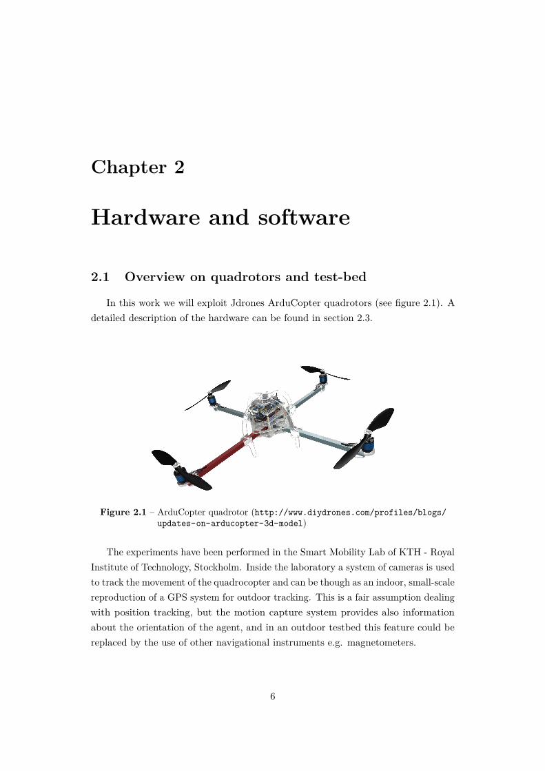
In this work we will exploit Jdrones ArduCopter quadrotors (see figure 2.1). Adetailed description of the hardware can be found in section 2.3.

Figure 2.1 – ArduCopter quadrotor (http://www.diydrones.com/profiles/blogs/updates-on-arducopter-3d-model)

The experiments have been performed in the Smart Mobility Lab of KTH - RoyalInstitute of Technology, Stockholm. Inside the laboratory a system of cameras is usedto track the movement of the quadrocopter and can be though as an indoor, small-scalereproduction of a GPS system for outdoor tracking. This is a fair assumption dealingwith position tracking, but the motion capture system provides also informationabout the orientation of the agent, and in an outdoor testbed this feature could bereplaced by the use of other navigational instruments e.g. magnetometers.

6

2.2 Principles of working

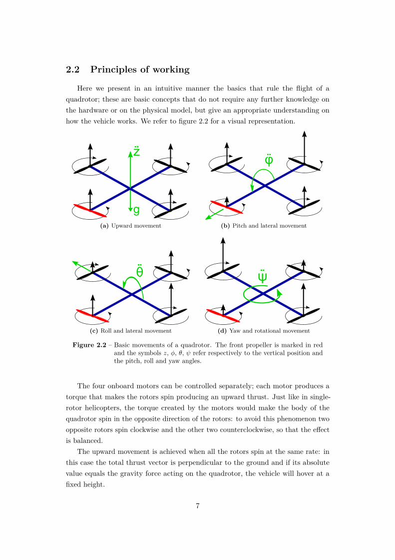
Here we present in an intuitive manner the basics that rule the flight of aquadrotor; these are basic concepts that do not require any further knowledge onthe hardware or on the physical model, but give an appropriate understanding onhow the vehicle works. We refer to figure 2.2 for a visual representation.

g

z..

(a) Upward movement

φ..

(b) Pitch and lateral movement

θ..

(c) Roll and lateral movement

..ψ

(d) Yaw and rotational movement

Figure 2.2 – Basic movements of a quadrotor. The front propeller is marked in redand the symbols z, φ, θ, ψ refer respectively to the vertical position andthe pitch, roll and yaw angles.

The four onboard motors can be controlled separately; each motor produces atorque that makes the rotors spin producing an upward thrust. Just like in single-rotor helicopters, the torque created by the motors would make the body of thequadrotor spin in the opposite direction of the rotors: to avoid this phenomenon twoopposite rotors spin clockwise and the other two counterclockwise, so that the effectis balanced.

The upward movement is achieved when all the rotors spin at the same rate: inthis case the total thrust vector is perpendicular to the ground and if its absolutevalue equals the gravity force acting on the quadrotor, the vehicle will hover at afixed height.

7

The lateral movement of the quadrotor is performed by decreasing the rate ofone rotor and increasing by the same amount the rate of the opposite one. In thisscenario the quadrotor will tilt towards the direction of the slow propeller and aslong as the total thrust do not variate, a lateral movement is achieved. This tiltingmovement is referred as pitch if the rotor that slows down is the front or the rearone, or roll if the rotor that slows down is a lateral one. However, since the vehicleis symmetrical with respect to its center of gravity, the choice of the orientation isnon-influential to the dynamics.

Finally, the rotational movement1, or yaw movement, can be obtained by slowingdown the spinning rate of two opposite propellers and increasing the spinning rate ofthe others by the same amount (so that the total thrust vector is not influenced). Inthis way, the quadrotor will rotate in the same direction as the slow propellers, infact as we have already stated, the torque of the motors produces a rotation of thebody in the opposite direction according to the third law of motion.

2.3 Introduction to the resources

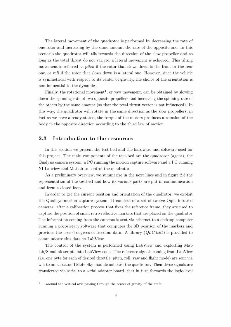
In this section we present the test-bed and the hardware and software used forthis project. The main components of the test-bed are the quadrotor (agent), theQualysis camera system, a PC running the motion capture software and a PC runningNI Labview and Matlab to control the quadrotor.

As a preliminary overview, we summarize in the next lines and in figure 2.3 therepresentation of the testbed and how its various parts are put in communicationand form a closed loop.

In order to get the current position and orientation of the quadrotor, we exploitthe Qualisys motion capture system. It consists of a set of twelve Oqus infraredcameras: after a calibration process that fixes the reference frame, they are used tocapture the position of small retro-reflective markers that are placed on the quadrotor.The information coming from the cameras is sent via ethernet to a desktop computerrunning a proprietary software that computes the 3D position of the markers andprovides the user 6 degrees of freedom data. A library (QLC.lvlib) is provided tocommunicate this data to LabView.

The control of the system is performed using LabView and exploiting Mat-lab/Simulink scripts into LabView code. The reference signals coming from LabView(i.e. one byte for each of desired throttle, pitch, roll, yaw and flight mode) are sent viawifi to an actuator TMote Sky module onboard the quadrotor. Then these signals aretransferred via serial to a serial adapter board, that in turn forwards the logic-level

1 around the vertical axis passing through the center of gravity of the craft.

8

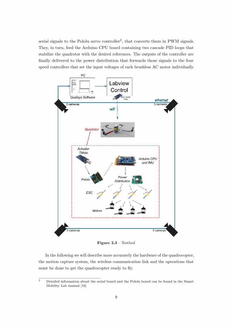
serial signals to the Pololu servo controller2, that converts them in PWM signals.They, in turn, feed the Arduino CPU board containing two cascade PID loops thatstabilize the quadrotor with the desired references. The outputs of the controller arefinally delivered to the power distribution that forwards those signals to the fourspeed controllers that set the input voltages of each brushless AC motor individually.

Figure 2.3 – Testbed

In the following we will describe more accurately the hardware of the quadrocopter,the motion capture system, the wireless communication link and the operations thatmust be done to get the quadrocopter ready to fly.

2 Detailed information about the serial board and the Pololu board can be found in the SmartMobility Lab manual [16]

9

2.4 Jdrones ArduCopter

Arducopter is a platform for multicopters and helicopters that provides bothmanual remote control and an autonomous flight system equipped with missionplanning, waypoints navigation and telemetry, managed via software from a groundstation.

The quadrocopter has been assembled from the ArduPilot Mega kit, containingthe Arduino controller board and the IMU board, and the JDrones ArduCopter kit,containing the frame, the motors, the speed controllers, the power distribution boardand the propellers. Detailed instruction on how to solder and assemble the parts ofthe kits are provided in the Wiki section of [17], we here present briefly how thesecomponents are connected and their role in the functioning of the quadrocopter.

2.4.1 ArduPilot Mega

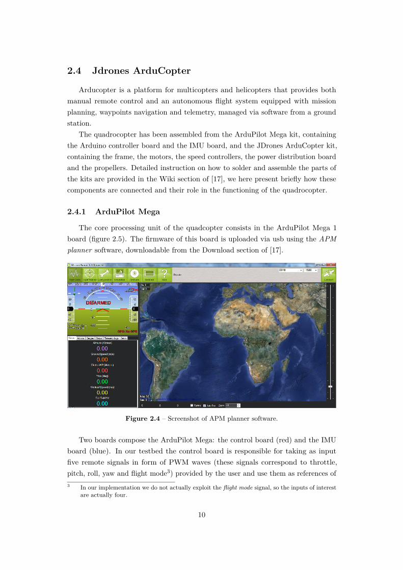
The core processing unit of the quadcopter consists in the ArduPilot Mega 1board (figure 2.5). The firmware of this board is uploaded via usb using the APMplanner software, downloadable from the Download section of [17].

Figure 2.4 – Screenshot of APM planner software.

Two boards compose the ArduPilot Mega: the control board (red) and the IMUboard (blue). In our testbed the control board is responsible for taking as inputfive remote signals in form of PWM waves (these signals correspond to throttle,pitch, roll, yaw and flight mode3) provided by the user and use them as references of3 In our implementation we do not actually exploit the flight mode signal, so the inputs of interest

are actually four.

10

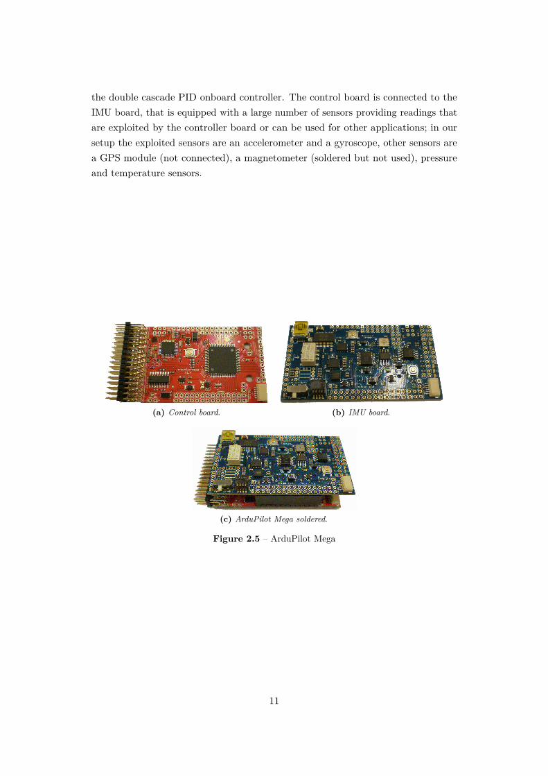
the double cascade PID onboard controller. The control board is connected to theIMU board, that is equipped with a large number of sensors providing readings thatare exploited by the controller board or can be used for other applications; in oursetup the exploited sensors are an accelerometer and a gyroscope, other sensors area GPS module (not connected), a magnetometer (soldered but not used), pressureand temperature sensors.

(a) Control board. (b) IMU board.

(c) ArduPilot Mega soldered.

Figure 2.5 – ArduPilot Mega

11

2.4.2 Arducopter frame, power distribution and motors

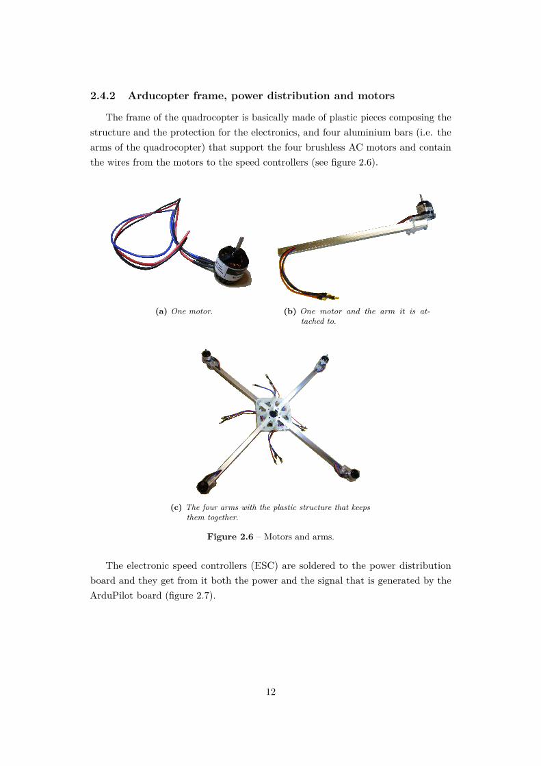
The frame of the quadrocopter is basically made of plastic pieces composing thestructure and the protection for the electronics, and four aluminium bars (i.e. thearms of the quadrocopter) that support the four brushless AC motors and containthe wires from the motors to the speed controllers (see figure 2.6).

(a) One motor. (b) One motor and the arm it is at-tached to.

(c) The four arms with the plastic structure that keepsthem together.

Figure 2.6 – Motors and arms.

The electronic speed controllers (ESC) are soldered to the power distributionboard and they get from it both the power and the signal that is generated by theArduPilot board (figure 2.7).

12

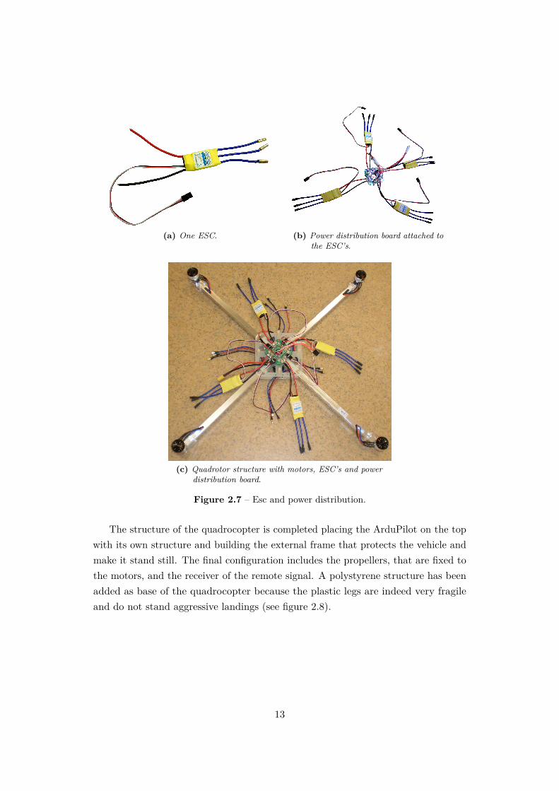
(a) One ESC. (b) Power distribution board attached tothe ESC’s.

(c) Quadrotor structure with motors, ESC’s and powerdistribution board.

Figure 2.7 – Esc and power distribution.

The structure of the quadrocopter is completed placing the ArduPilot on the topwith its own structure and building the external frame that protects the vehicle andmake it stand still. The final configuration includes the propellers, that are fixed tothe motors, and the receiver of the remote signal. A polystyrene structure has beenadded as base of the quadrocopter because the plastic legs are indeed very fragileand do not stand aggressive landings (see figure 2.8).

13

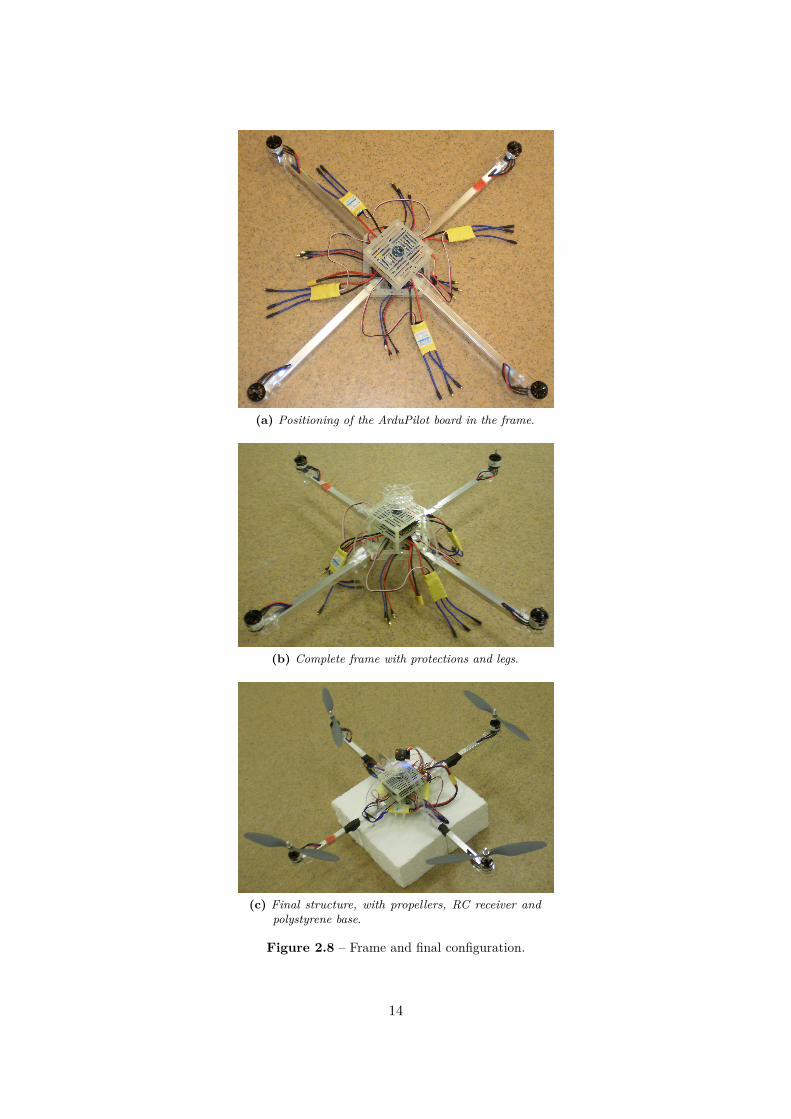
(a) Positioning of the ArduPilot board in the frame.

(b) Complete frame with protections and legs.

(c) Final structure, with propellers, RC receiver andpolystyrene base.

Figure 2.8 – Frame and final configuration.

14

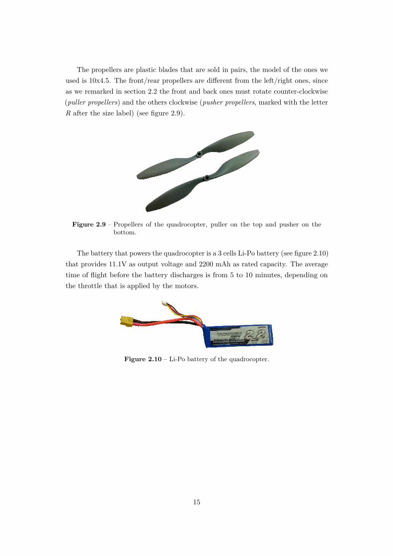
The propellers are plastic blades that are sold in pairs, the model of the ones weused is 10x4.5. The front/rear propellers are different from the left/right ones, sinceas we remarked in section 2.2 the front and back ones must rotate counter-clockwise(puller propellers) and the others clockwise (pusher propellers, marked with the letterR after the size label) (see figure 2.9).

Figure 2.9 – Propellers of the quadrocopter, puller on the top and pusher on thebottom.

The battery that powers the quadrocopter is a 3 cells Li-Po battery (see figure 2.10)that provides 11.1V as output voltage and 2200 mAh as rated capacity. The averagetime of flight before the battery discharges is from 5 to 10 minutes, depending onthe throttle that is applied by the motors.

Figure 2.10 – Li-Po battery of the quadrocopter.

15

2.5 Qualysis motion capture system

(a) Qualisys logo. (b) QTM logo.

Figure 2.11 – Qualysis and Qualisys Track Manager logos

The motion capture (MoCap) system provided by Qualisys consists in a certainnumber of IR cameras, each of them equipped with an infrared flash. The light ofthe flashes is reflected by small reflective balls (markers) that are placed in advanceon the objects we are interested in tracking, and the cameras capture these reflectedbeams and compute relative position and size of the markers. After the informationcollected by every camera is transmitted via ethernet to a computer running theQualisys Tracking Software (QTM) and the position of the cameras being known, the3D position of the markers is computed by the software. If a group of markers havebeen previously gathered by the user forming a body, then the software is able totrack not just the position of the markers, but also the 3D position and orientationof the body when it moves in the workspace.

In order for the cameras to accurately compute the position of the markers, acalibration process has to be carried out before data collection. This is performed byplacing an L-shaped tool representing the reference system on the ground, and, afterstarting the procedure in the QTM software, carrying around a calibration wand andmoving it in all directions for a preset time (see the tools in figure 2.12).

Figure 2.12 – Wand and reference system (www.qualysis.com).

16

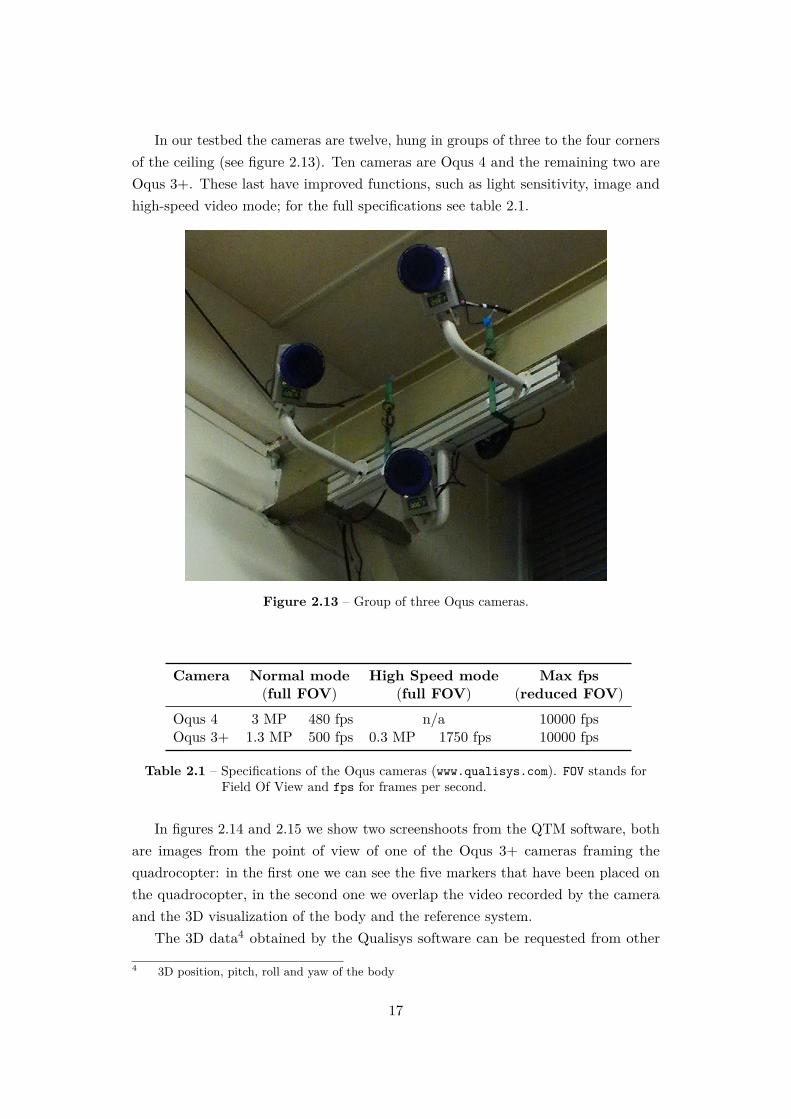
In our testbed the cameras are twelve, hung in groups of three to the four cornersof the ceiling (see figure 2.13). Ten cameras are Oqus 4 and the remaining two areOqus 3+. These last have improved functions, such as light sensitivity, image andhigh-speed video mode; for the full specifications see table 2.1.

Figure 2.13 – Group of three Oqus cameras.

Camera Normal mode High Speed mode Max fps(full FOV) (full FOV) (reduced FOV)

Oqus 4 3 MP 480 fps n/a 10000 fpsOqus 3+ 1.3 MP 500 fps 0.3 MP 1750 fps 10000 fps

Table 2.1 – Specifications of the Oqus cameras (www.qualisys.com). FOV stands forField Of View and fps for frames per second.

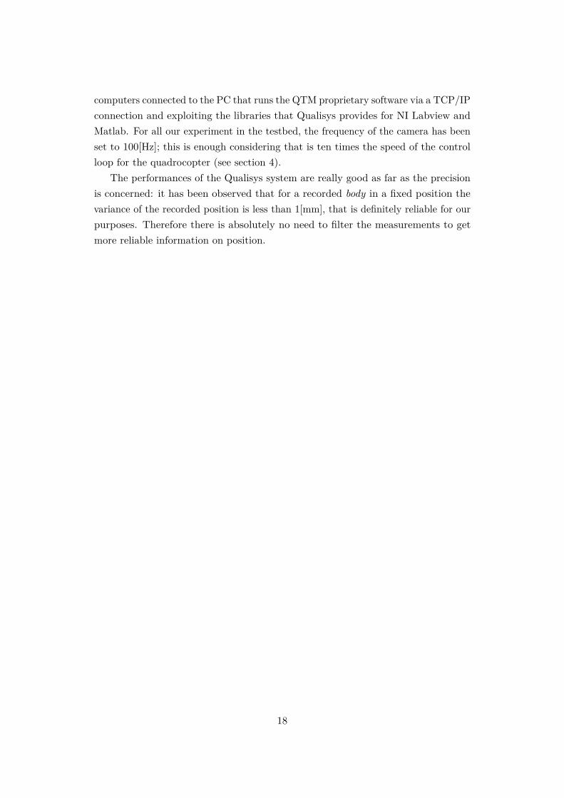
In figures 2.14 and 2.15 we show two screenshoots from the QTM software, bothare images from the point of view of one of the Oqus 3+ cameras framing thequadrocopter: in the first one we can see the five markers that have been placed onthe quadrocopter, in the second one we overlap the video recorded by the cameraand the 3D visualization of the body and the reference system.

The 3D data4 obtained by the Qualisys software can be requested from other

4 3D position, pitch, roll and yaw of the body

17

computers connected to the PC that runs the QTM proprietary software via a TCP/IPconnection and exploiting the libraries that Qualisys provides for NI Labview andMatlab. For all our experiment in the testbed, the frequency of the camera has beenset to 100[Hz]; this is enough considering that is ten times the speed of the controlloop for the quadrocopter (see section 4).

The performances of the Qualisys system are really good as far as the precisionis concerned: it has been observed that for a recorded body in a fixed position thevariance of the recorded position is less than 1[mm], that is definitely reliable for ourpurposes. Therefore there is absolutely no need to filter the measurements to getmore reliable information on position.

18

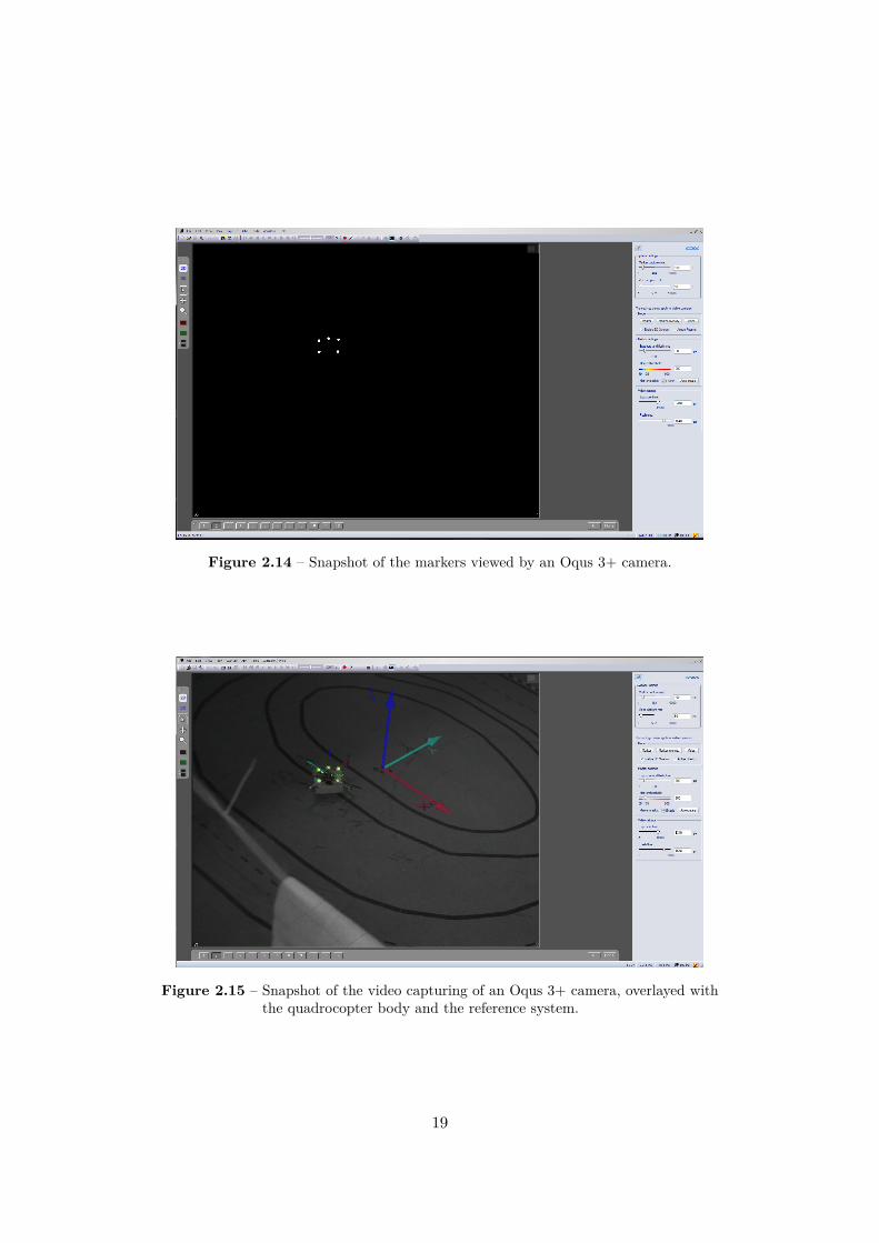
Figure 2.14 – Snapshot of the markers viewed by an Oqus 3+ camera.

Figure 2.15 – Snapshot of the video capturing of an Oqus 3+ camera, overlayed withthe quadrocopter body and the reference system.

19

2.6 Communication link

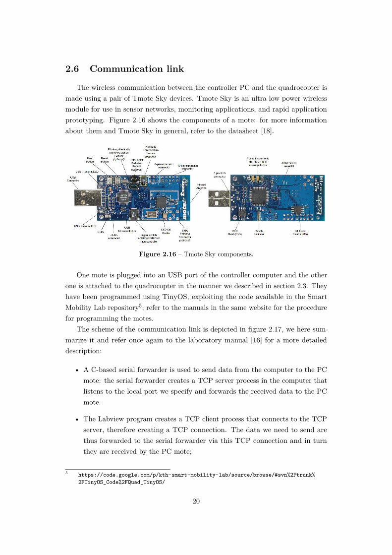
The wireless communication between the controller PC and the quadrocopter ismade using a pair of Tmote Sky devices. Tmote Sky is an ultra low power wirelessmodule for use in sensor networks, monitoring applications, and rapid applicationprototyping. Figure 2.16 shows the components of a mote: for more informationabout them and Tmote Sky in general, refer to the datasheet [18].

Figure 2.16 – Tmote Sky components.

One mote is plugged into an USB port of the controller computer and the otherone is attached to the quadrocopter in the manner we described in section 2.3. Theyhave been programmed using TinyOS, exploiting the code available in the SmartMobility Lab repository5; refer to the manuals in the same website for the procedurefor programming the motes.

The scheme of the communication link is depicted in figure 2.17, we here sum-marize it and refer once again to the laboratory manual [16] for a more detaileddescription:

• A C-based serial forwarder is used to send data from the computer to the PCmote: the serial forwarder creates a TCP server process in the computer thatlistens to the local port we specify and forwards the received data to the PCmote.

• The Labview program creates a TCP client process that connects to the TCPserver, therefore creating a TCP connection. The data we need to send arethus forwarded to the serial forwarder via this TCP connection and in turnthey are received by the PC mote;

5 https://code.google.com/p/kth-smart-mobility-lab/source/browse/#svn%2Ftrunk%2FTinyOS_Code%2FQuad_TinyOS/

20

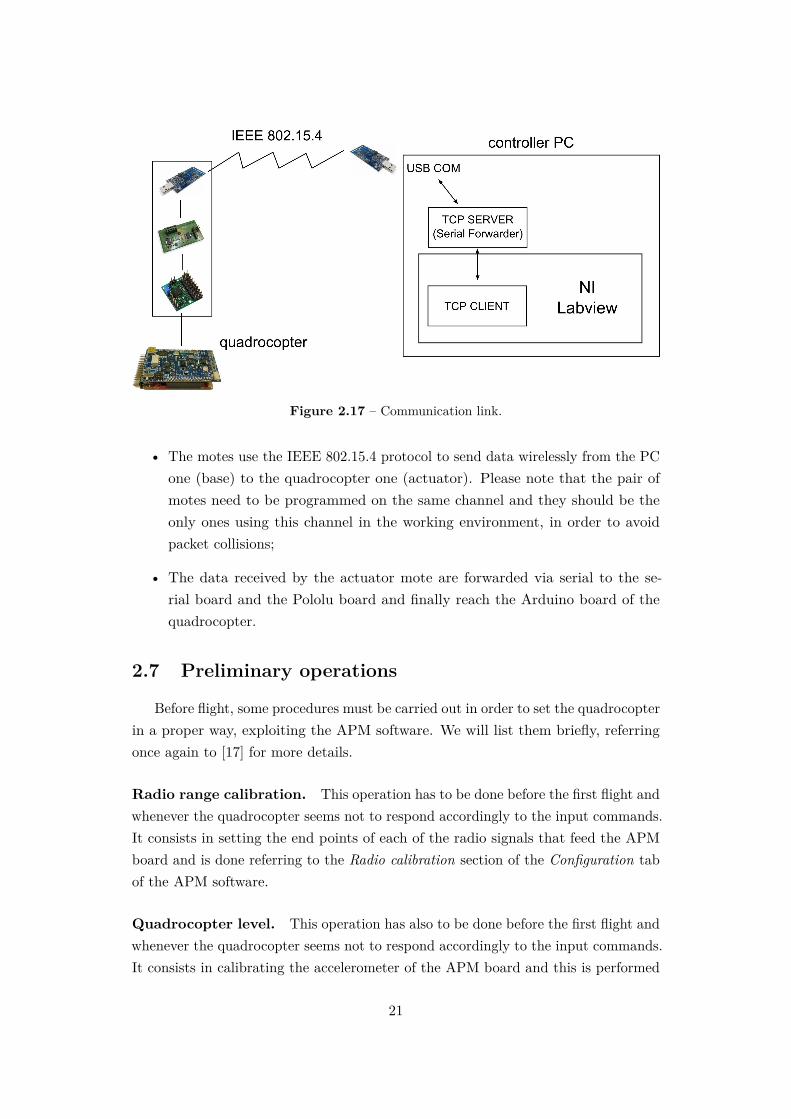
Figure 2.17 – Communication link.

• The motes use the IEEE 802.15.4 protocol to send data wirelessly from the PCone (base) to the quadrocopter one (actuator). Please note that the pair ofmotes need to be programmed on the same channel and they should be theonly ones using this channel in the working environment, in order to avoidpacket collisions;

• The data received by the actuator mote are forwarded via serial to the se-rial board and the Pololu board and finally reach the Arduino board of thequadrocopter.

2.7 Preliminary operations

Before flight, some procedures must be carried out in order to set the quadrocopterin a proper way, exploiting the APM software. We will list them briefly, referringonce again to [17] for more details.

Radio range calibration. This operation has to be done before the first flight andwhenever the quadrocopter seems not to respond accordingly to the input commands.It consists in setting the end points of each of the radio signals that feed the APMboard and is done referring to the Radio calibration section of the Configuration tabof the APM software.

Quadrocopter level. This operation has also to be done before the first flight andwhenever the quadrocopter seems not to respond accordingly to the input commands.It consists in calibrating the accelerometer of the APM board and this is performed

21

automatically by the software (Level section of the Configuration tab): the user onlyneeds to orientate the APM accordingly to the onscreen instructions and keep it stillwhile the software records the data it needs.

Esc calibration. This operation has to be done right after building the quadro-copter and whenever we suspect that the speed of the motors are not correctlybalanced. It aims to make the speed controllers react in the same fashion to theAPM and to the RC commands. Automatic calibration is the easiest way to performit, since it is just necessary to hear the tones emitted by the APM and move theremote sticks6 as a consequence.

Onboard PIDs. This operation is not strictly necessary, but we observed that itprovides better results in the height control. Since the motors the quadrocopter carriesare quite powerful in respect to the weight of the vehicle itself, it is recommended tomodify the proportional gain parameter of the stabilizing onboard controller.7 Thedefault parameter is the one for medium-size motors (0.110), we decided to switch itto 0.100, that is the mean value between the ones recommended for medium-size andlarge-size motors.

6 or changing the input values if we are using remote Labview control7 This can be done via the APM software, in the section Configuration → Standard parameters

→ Arducopter PIDs → Stabilization, angular rate control

22

Chapter 3

Quadrotor modeling andidentification

3.1 Quadrotor mathematical model

We want to provide here a mathematical model of the quadrotor, exploitingNewton and Euler equations for the 3D motion of a rigid body, i.e. the so-calledFirst principles modeling) (see for instance [19], [20], [21]). The goal of this sectionis obtaining a deeper understanding of the dynamics of the quadrotor and provide amodel that is enough reliable for simulating its behavior.

We start by defining two reference frames: the body reference frame (B), that isthe local reference system of the quadrotor, and the Earth inertial reference frame.In the continuation, all the quantities referring to the body and Earth frames will bewritten with B or E superscripts respectively.

Let us denominate as

qE , [ x y z φ θ ψ ]T

the vector containing the linear and angular position of the quadrotor in the earthframe and

qB , [ u v w p q r ]T

the vector containing the linear and angular velocities in the body frame. From 3Dbody dynamics, it follows that the two reference frames are linked by the following

23

relations (see [19], [22]):x

y

z

= ERB

u

v

w

,cψcθ −sψcφ + cφsθsφ sψsφ + cψsθcφ

sψcθ cψcφ + sψsθsφ −cψsφ + sψsθcφ

−sθ cθsφ cθcφ

u

v

w

φ

θ

ψ

= ETB

p

q

r

,

1 sφtθ cφtθ

0 cφ −sφ0 sφ/cθ cφ/cθ

p

q

r

,(3.1)

so we get

qE =

ERB 03×3

03×3ETB

qB (3.2)

We indicated for the sake of brevity sin(α), cos(α) and tan(α) as sα, cα and tα, fora generic angle α.

Newton’s law states the following matrix relation for the total force acting onthe quadrotor in the body frame:

FB = mV B + ΩB ×mV B, (3.3)

where FB ∈ R3×1 is the total force, m is the mass of the quadrotor, V B ∈ R3×1 isthe linear velocity of the quadrotor and ΩB ∈ R3×1 is the angular velocity of thequadrotor. Euler’s equation gives the total torque applied to the quadrotor:

τB = JΩB + ΩB × JΩB, (3.4)

where τB ∈ R3×1 is the total torque and J ∈ R3×3 is the diagonal inertia matrix.The kinematic equations (3.3) and (3.4) stand as long as we assume that the origin

and the axes of the body frame coincide with the center of mass of the quadrotorand the axes of inertia, respectively.

Let us now consider the dynamics of the quadrotor, i.e. how the total force andthe total torque vectors are composed.

Gravity. Gravity has effect on the total force and its direction is along the z axisof the earth frame1:

FBgr = BRE FEgr = (ERB)T

00−mg

=

mgsθ

−mgcθsφ−mgcθcφ

(3.5)

1 Since BRE is a rotational matrix, it is orthogonal, i.e. its inverse equals its transposed.

24

Gyroscopic effects. Gyroscopic contributions are present if the total sum of therotational speeds of the rotors ΩRtot = −ΩR1 + ΩR2 − ΩR3 + ΩR4 is not zero andthey influence the total torque adding the following term (see [19], [23]):

τBgyro = JRot

−qp

0

ΩRtot, (3.6)

where JRot is the moment of inertia of any rotor.

Control inputs. We here consider the inputs that can be applied to the system inorder to control the behavior of the quadrotor. The rotors are four and the degreesof freedom we control are as many: commonly, the control inputs that are consideredare one for the vertical thrust and one for each of the angular movements. Let usconsider the values of the input forces and torques proportional to the squared speedsof the rotors (see [19] for aerodynamic motivations); their values are the following:

U1 = b(Ω2R1 + Ω2

R2 + Ω2R3 + Ω2

R4)

U2 = bl(Ω2R3 − Ω2

R1)

U3 = bl(Ω2R4 − Ω2

R2)

U4 = d(−Ω2R1 + Ω2

R2 − Ω2R3 + Ω2

R4),

(3.7)

wherer l is the distance between any rotor and the center of the drone, ΩRi is theangular speed of the i-th rotor, b is the thrust factor, d is the drag factor. The inputsUi can be directly related, at least on first approximation, respectively the vertical,pitch, roll and yaw accelerations (see also the oncoming equation (3.9)).

As we summarize the above-obtained relations in one matrix equation we get 2

mI3×3 03×3

03×3 J

qB +

03×3 −Sk(mV B)03×3 −Sk(JΩB)

qB =

FB

τB

, (3.8)

2 We remind that the general cross product a× b ,

[a1a2a3

]×

[b1b2b3

]can be written as

Sk(a) b = −Sk(b) a, where Sk(a) is the skew-symmetric matrix

[ 0 −a3 a2a3 0 −a1−a2 a1 0

]

25

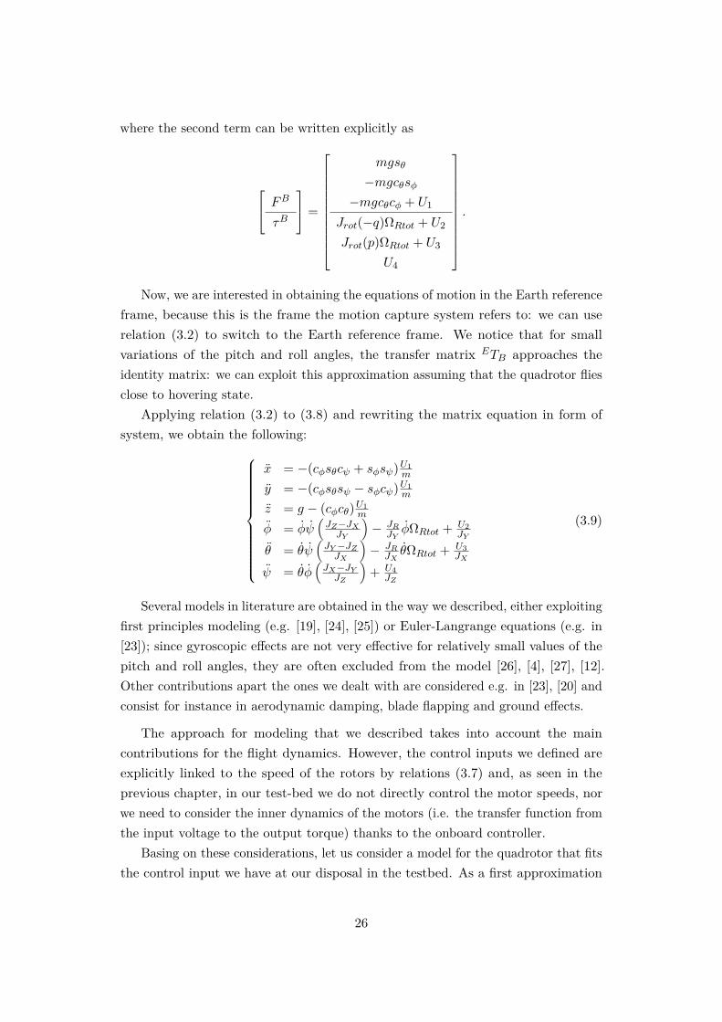
where the second term can be written explicitly as

FB

τB

=

mgsθ

−mgcθsφ−mgcθcφ + U1

Jrot(−q)ΩRtot + U2

Jrot(p)ΩRtot + U3

U4

.

Now, we are interested in obtaining the equations of motion in the Earth referenceframe, because this is the frame the motion capture system refers to: we can userelation (3.2) to switch to the Earth reference frame. We notice that for smallvariations of the pitch and roll angles, the transfer matrix ETB approaches theidentity matrix: we can exploit this approximation assuming that the quadrotor fliesclose to hovering state.

Applying relation (3.2) to (3.8) and rewriting the matrix equation in form ofsystem, we obtain the following:

x = −(cφsθcψ + sφsψ)U1m

y = −(cφsθsψ − sφcψ)U1m

z = g − (cφcθ)U1m

φ = φψ(JZ−JXJY

)− JR

JYφΩRtot + U2

JY

θ = θψ(JY −JZJX

)− JR

JXθΩRtot + U3

JX

ψ = θφ(JX−JYJZ

)+ U4

JZ

(3.9)

Several models in literature are obtained in the way we described, either exploitingfirst principles modeling (e.g. [19], [24], [25]) or Euler-Langrange equations (e.g. in[23]); since gyroscopic effects are not very effective for relatively small values of thepitch and roll angles, they are often excluded from the model [26], [4], [27], [12].Other contributions apart the ones we dealt with are considered e.g. in [23], [20] andconsist for instance in aerodynamic damping, blade flapping and ground effects.

The approach for modeling that we described takes into account the maincontributions for the flight dynamics. However, the control inputs we defined areexplicitly linked to the speed of the rotors by relations (3.7) and, as seen in theprevious chapter, in our test-bed we do not directly control the motor speeds, norwe need to consider the inner dynamics of the motors (i.e. the transfer function fromthe input voltage to the output torque) thanks to the onboard controller.

Basing on these considerations, let us consider a model for the quadrotor that fitsthe control input we have at our disposal in the testbed. As a first approximation

26

we can state that the values for throttle, pitch, roll and yaw movements we send tothe quadrotor are the control inputs Ui we described in the previous section. Sincein equation 3.9 the values of inertia are unknown3 and willing to understand howthe behavior of the actual system relates to those equations, we now aim to retrievethe relations between our inputs and effective vertical thrust, pitch, roll and yaw inthe form of transfer functions (t.f.).

These transfer functions can be estimated thanks to the knowledge of the inputs(expressed as byte values) and outputs of the system (expressed as height wrt thethrottle input and as angular value in degrees wrt the pitch, roll and yaw), and thisprocess will be content of the following section.

3.2 Transfer functions identification

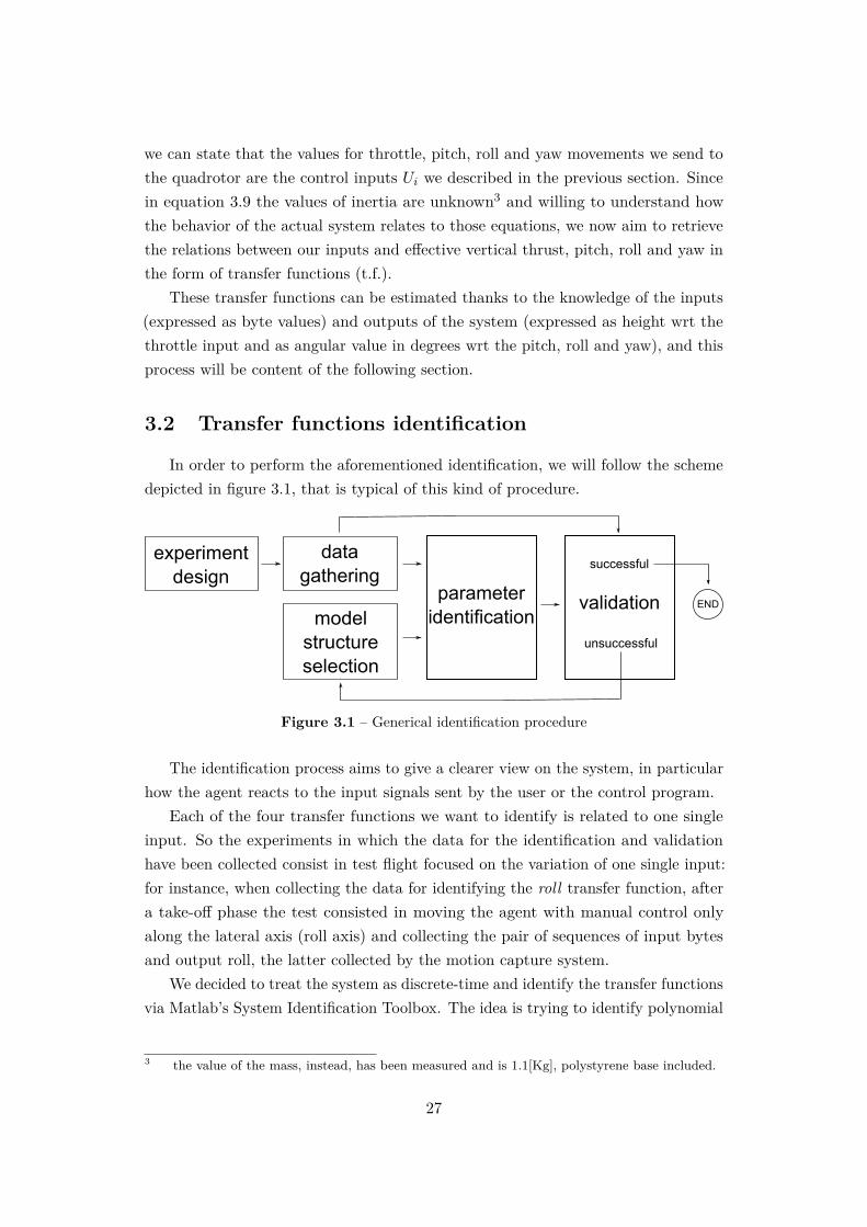
In order to perform the aforementioned identification, we will follow the schemedepicted in figure 3.1, that is typical of this kind of procedure.

experimentdesign

datagathering

modelstructureselection

parameteridentification

validation

successful

unsuccessful

END

Figure 3.1 – Generical identification procedure

The identification process aims to give a clearer view on the system, in particularhow the agent reacts to the input signals sent by the user or the control program.

Each of the four transfer functions we want to identify is related to one singleinput. So the experiments in which the data for the identification and validationhave been collected consist in test flight focused on the variation of one single input:for instance, when collecting the data for identifying the roll transfer function, aftera take-off phase the test consisted in moving the agent with manual control onlyalong the lateral axis (roll axis) and collecting the pair of sequences of input bytesand output roll, the latter collected by the motion capture system.

We decided to treat the system as discrete-time and identify the transfer functionsvia Matlab’s System Identification Toolbox. The idea is trying to identify polynomial

3 the value of the mass, instead, has been measured and is 1.1[Kg], polystyrene base included.

27

models of the form Output-Error (OE) i.e. models with the generic structure

y(t) = B(z)F (z)u(t− nd) + e(t),

where B(z) and F (z) are the polynomials to identify, nd is the input-output delayexpressed as number of samples and e(t) is white noise. We chose this kind of modelsince we are not interested in the structure of the noise, that we indeed assume tobe white, and since under hypothesis of small angular values, equations (3.9) let usrelate the input and output at our disposal in the following way:

z ≈ g − U1m

φ ≈ U2JY

θ ≈ U3JX

ψ ≈ U4JZ

(3.10)

so a linear input-output transfer function can be considered a fair approximation aslong as the previous ones stand.

Let us now describe the procedure for identification; for each unknown transferfunction:

• The collected data (both inputs and outputs) have been divided into identifica-tion and validation data;

• Two iddata objects are created, one for the identification and one for thevalidation;

• The number of poles, zeroes and delay samples is set and Matlab function oe

is run on the data. This function is based on the prediction error minimizationmethod (PEM): starting from a chosen structure of the model, a predictor of thepresent output is built, based on past inputs and outputs. The PEM methodestimates the parameters of the model minimizing the prediction errors, i.e.minimizing a cost function that depends on these errors, that in turn depend onthe unknown parameters and the measured outputs. For a detailed descriptionand analysis of the PEM method and system identification in general, see [28];

• The obtained transfer function is tested on the validation data using thecompare function of the toolbox, that gives both a numerical fit and a visualdepiction of the suitability of the estimated model;

• If the results are not satisfactory we change the order of the transfer functionand repeat the procedure.

28

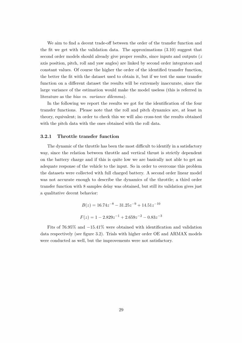
We aim to find a decent trade-off between the order of the transfer function andthe fit we get with the validation data. The approximations (3.10) suggest thatsecond order models should already give proper results, since inputs and outputs (zaxis position, pitch, roll and yaw angles) are linked by second order integrators andconstant values. Of course the higher the order of the identified transfer function,the better the fit with the dataset used to obtain it, but if we test the same transferfunction on a different dataset the results will be extremely inaccurate, since thelarge variance of the estimation would make the model useless (this is referred inliterature as the bias vs. variance dilemma).

In the following we report the results we got for the identification of the fourtransfer functions. Please note that the roll and pitch dynamics are, at least intheory, equivalent; in order to check this we will also cross-test the results obtainedwith the pitch data with the ones obtained with the roll data.

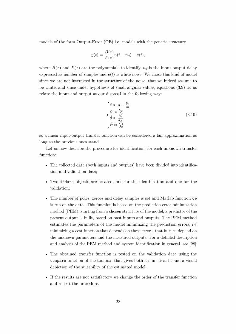
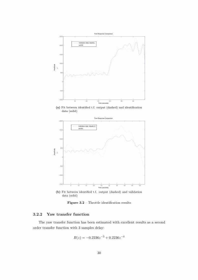
3.2.1 Throttle transfer function

The dynamic of the throttle has been the most difficult to identify in a satisfactoryway, since the relation between throttle and vertical thrust is strictly dependenton the battery charge and if this is quite low we are basically not able to get anadequate response of the vehicle to the input. So in order to overcome this problemthe datasets were collected with full charged battery. A second order linear modelwas not accurate enough to describe the dynamics of the throttle; a third ordertransfer function with 8 samples delay was obtained, but still its validation gives justa qualitative decent behavior:

B(z) = 16.74z−8 − 31.25z−9 + 14.51z−10

F (z) = 1− 2.829z−1 + 2.659z−2 − 0.83z−3

Fits of 76.95% and −15.41% were obtained with identification and validationdata respectively (see figure 3.2). Trials with higher order OE and ARMAX modelswere conducted as well, but the improvements were not satisfactory.

29

10 20 30 40 50 60-1000

-500

0

500

1000

1500

2000

2500

y1

Time Response Comparison

Time (seconds)

Am

plit

ud

e

Validation data: dataALL

oe338

(a) Fit between identified t.f. output (dashed) and identificationdata (solid)

5 10 15 20 25 30 35 40 45 50-1500

-1000

-500

0

500

1000

1500

2000

y1

Time Response Comparison

Time (seconds)

Am

plit

ud

e

Validation data: dataALL2

oe338

(b) Fit between identified t.f. output (dashed) and validationdata (solid)

Figure 3.2 – Throttle identification results

3.2.2 Yaw transfer function

The yaw transfer function has been estimated with excellent results as a secondorder transfer function with 3 samples delay:

B(z) = −0.2236z−3 + 0.2236z−4

30

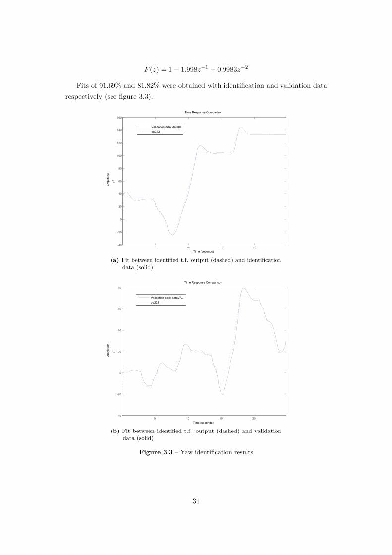
F (z) = 1− 1.998z−1 + 0.9983z−2

Fits of 91.69% and 81.82% were obtained with identification and validation datarespectively (see figure 3.3).

5 10 15 20-40

-20

0

20

40

60

80

100

120

140

160

y1Time Response Comparison

Time (seconds)

Am

plit

ud

e

Validation data: dataID

oe223

(a) Fit between identified t.f. output (dashed) and identificationdata (solid)

5 10 15 20-40

-20

0

20

40

60

80

y1

Time Response Comparison

Time (seconds)

Am

plit

ud

e

Validation data: dataVAL

oe223

(b) Fit between identified t.f. output (dashed) and validationdata (solid)

Figure 3.3 – Yaw identification results

31

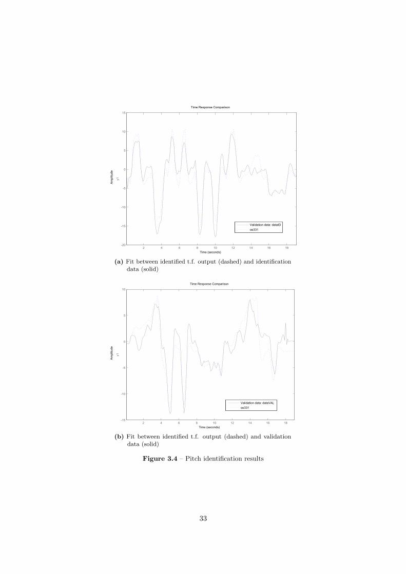
3.2.3 Pitch and Roll transfer functions

Both for the pitch and roll transfer functions we get satisfactory results. Eventhough second order transfer functions provided a visible concordance between inputsand outputs, we decided that it was worthy to keep as valid third order t.f.’s (withone delay sample), since the fits with the validation data were more than double theones with second order t.f.’s.

For the pitch we obtain:

B(z) = 0.09248z−1 − 0.3035z−2 + 0.2111z−3

F (z) = 1− 2.295z−1 + 1.841z−2 − 0.5439z−3

Fits of 64.78% and 48.31% were obtained with identification and validation datarespectively (see figure 3.4).

For the roll we obtain:

B(z) = 0.09248z−1 − 0.3035z−2 + 0.2111z−3

F (z) = 1− 2.295z−1 + 1.841z−2 − 0.5439z−3

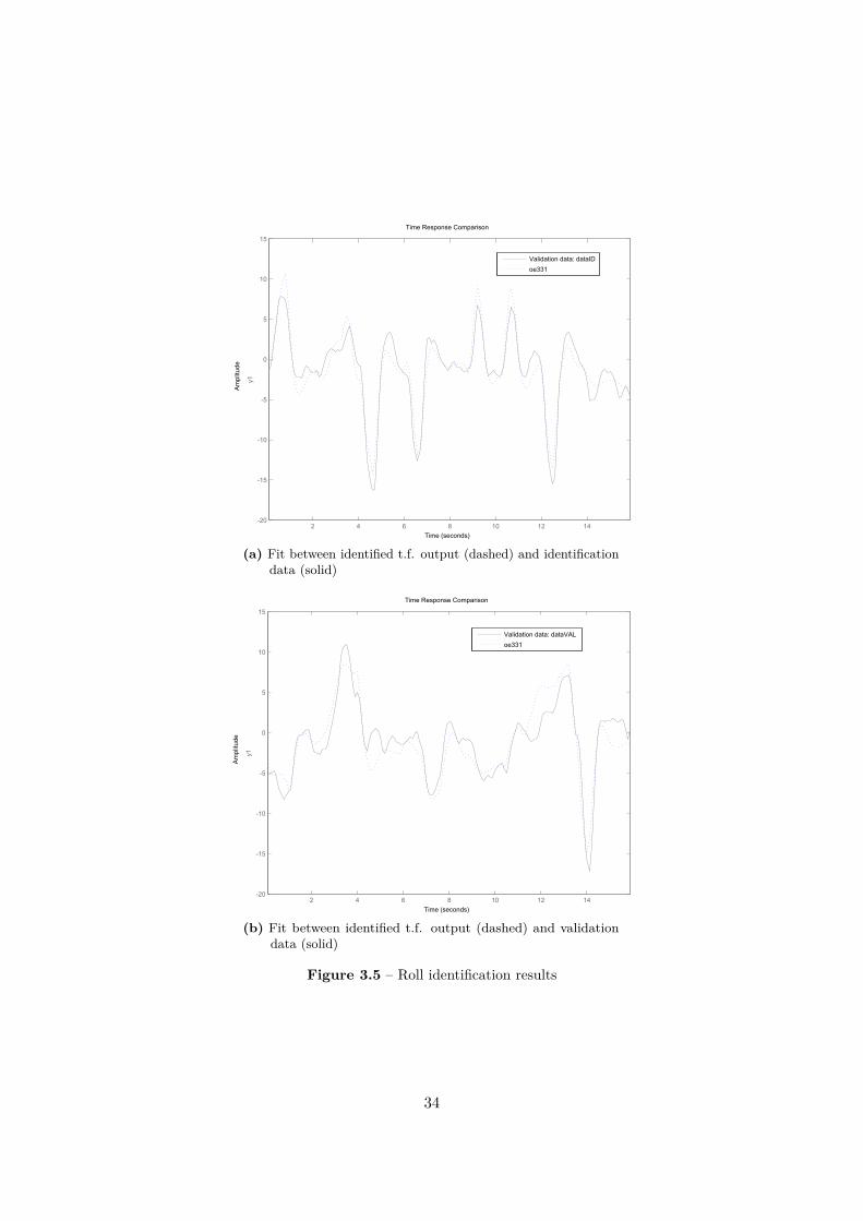
Fits of 67.15% and 54.5% were obtained with identification and validation datarespectively (see figure 3.5).

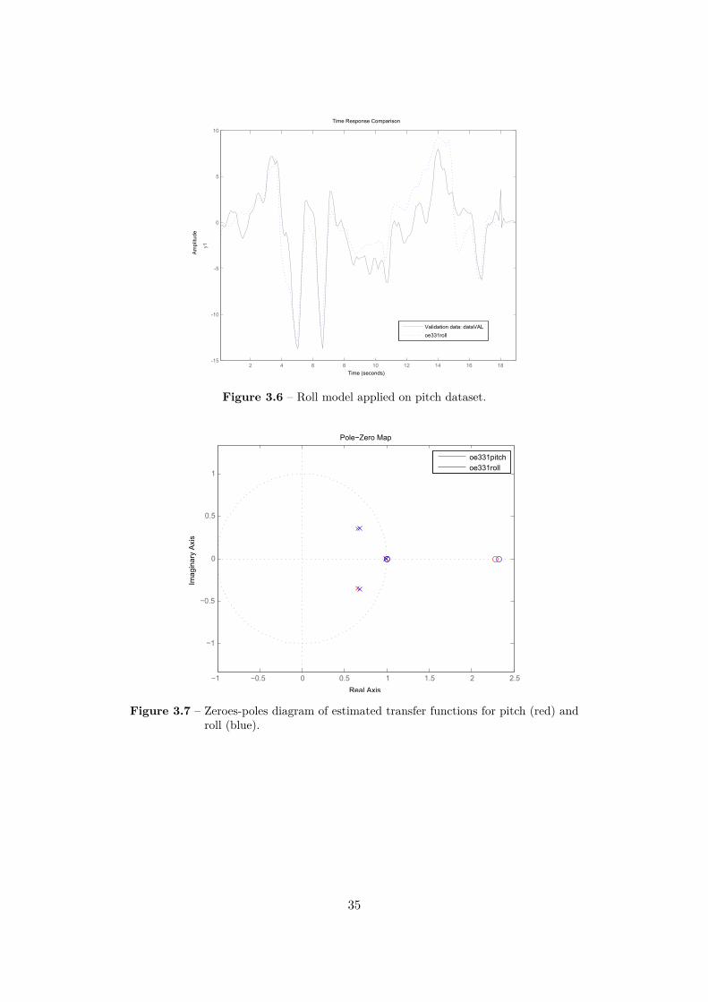
In order to compare the t.f.’s for the pitch and roll dynamics we applied the modelobtained for the roll4 to the validation data of the pitch. We obtained a fit of 42.86%(see figure 3.6), that is very close to the one we had with the pitch model itself.

From the zeroes-poles diagrams (3.7) of the two transfer functions we can seethat their positions are really close so the dynamics for the pitch and roll can indeedbe considered equivalent to a good approximation.

4 The sign of the transfer function had to be inverted in order to get concordance

32

2 4 6 8 10 12 14 16 18-20

-15

-10

-5

0

5

10

15y1

Time Response Comparison

Time (seconds)

Am

plit

ud

e

Validation data: dataID

oe331

(a) Fit between identified t.f. output (dashed) and identificationdata (solid)

2 4 6 8 10 12 14 16 18-15

-10

-5

0

5

10

y1

Time Response Comparison

Time (seconds)

Am

plit

ud

e

Validation data: dataVAL

oe331

(b) Fit between identified t.f. output (dashed) and validationdata (solid)

Figure 3.4 – Pitch identification results

33

2 4 6 8 10 12 14-20

-15

-10

-5

0

5

10

15y1

Time Response Comparison

Time (seconds)

Am

plit

ud

e

Validation data: dataID

oe331

(a) Fit between identified t.f. output (dashed) and identificationdata (solid)

2 4 6 8 10 12 14-20

-15

-10

-5

0

5

10

15

y1

Time Response Comparison

Time (seconds)

Am

plit

ud

e

Validation data: dataVAL

oe331

(b) Fit between identified t.f. output (dashed) and validationdata (solid)

Figure 3.5 – Roll identification results

34

2 4 6 8 10 12 14 16 18-15

-10

-5

0

5

10

y1

Time Response Comparison

Time (seconds)

Am

plit

ud

e

Validation data: dataVAL

oe331roll

Figure 3.6 – Roll model applied on pitch dataset.

Pole−Zero Map

Real Axis

Imag

inar

y A

xis

−1 −0.5 0 0.5 1 1.5 2 2.5

−1

−0.5

0

0.5

1

oe331pitch

oe331roll

Figure 3.7 – Zeroes-poles diagram of estimated transfer functions for pitch (red) androll (blue).

35

The identification results show that the less noisy dynamic is the one of the yawangle, whereas the relation between the throttle input and the vertical position/ac-celeration is not straightforward and is affected by significant disturbances. Theseconsiderations will match with the control presented in next chapter, since if on theone hand the yaw is easily controllable with a proportional controller and the pitchand roll controls are satisfactory, on the other hand the height control is the mostchallenging, even if it does not affect critically the success of the experiments.

36

Chapter 4

Quadrotor control

In this section we will present the controller that has been designed and imple-mented in the testbed. Since the setup allows online tuning of the controllers withsafety precautions that are not too onerous, we decided to bypass the tuning on asimulated model, that would request to be refined online anyway, once implementedin the testbed.

4.1 Controller description

The aim of the controller is point-to-point navigation with obstacle avoidance.The controller is structured in a layered fashion, as we can see in figure 4.1:

• The most external control is the path planning, i.e. the computation of apath to the destination point that provides obstacle avoidance. This is doneexploiting the implementation of a navigation-function based control in Matlab.The path planning provides the waypoints that have to be followed by theagent and deals with the switching from one waypoint to the following wheneither a temporal or a positional condition is triggered.

• The references provided by the path planning feed four PID controllers1, onefor each of the throttle, pitch, roll and yaw movements of the quadrotor andthe output of the controllers is sent via wireless to the agent.

• As we already mentioned, the onboard controllers of the quadrotor stabilize itsposition exploiting the references for throttle, pitch, roll and yaw.

• Additional control is also provided, in the form of a safety control that makesthe quadrotor land if it approaches non-fly zones and a manual control, that

1 We will not focus on the theory of the PID control, referring to any basic textbook of automaticcontrol for clarifications.

37

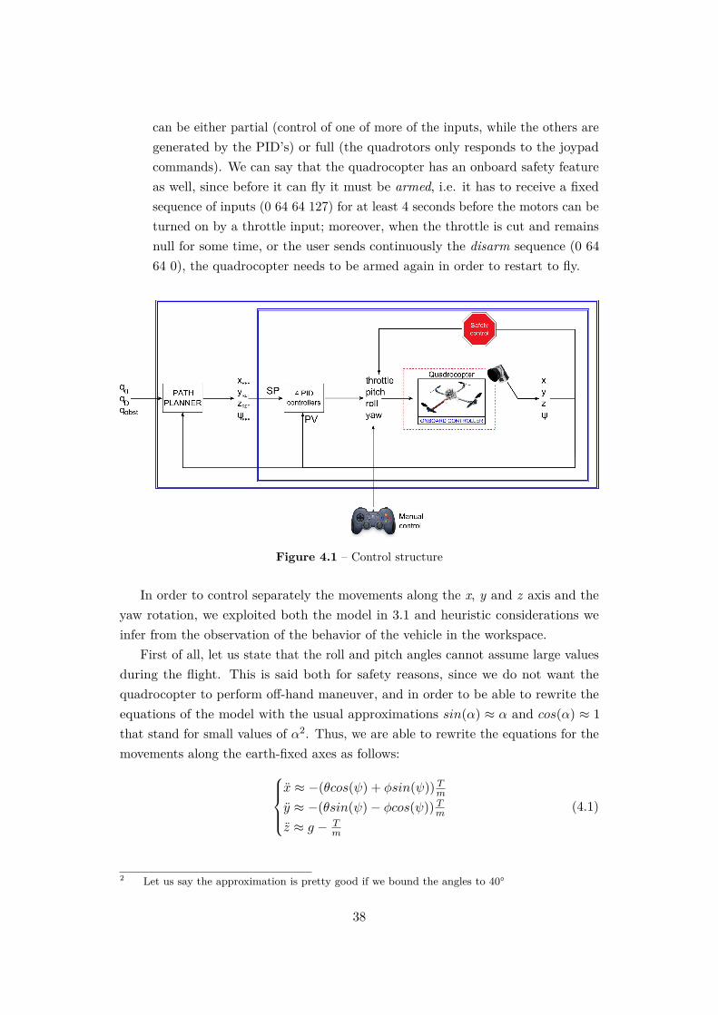
can be either partial (control of one of more of the inputs, while the others aregenerated by the PID’s) or full (the quadrotors only responds to the joypadcommands). We can say that the quadrocopter has an onboard safety featureas well, since before it can fly it must be armed, i.e. it has to receive a fixedsequence of inputs (0 64 64 127) for at least 4 seconds before the motors can beturned on by a throttle input; moreover, when the throttle is cut and remainsnull for some time, or the user sends continuously the disarm sequence (0 6464 0), the quadrocopter needs to be armed again in order to restart to fly.

Figure 4.1 – Control structure

In order to control separately the movements along the x, y and z axis and theyaw rotation, we exploited both the model in 3.1 and heuristic considerations weinfer from the observation of the behavior of the vehicle in the workspace.

First of all, let us state that the roll and pitch angles cannot assume large valuesduring the flight. This is said both for safety reasons, since we do not want thequadrocopter to perform off-hand maneuver, and in order to be able to rewrite theequations of the model with the usual approximations sin(α) ≈ α and cos(α) ≈ 1that stand for small values of α2. Thus, we are able to rewrite the equations for themovements along the earth-fixed axes as follows:

x ≈ −(θcos(ψ) + φsin(ψ)) Tmy ≈ −(θsin(ψ)− φcos(ψ)) Tmz ≈ g − T

m

(4.1)

2 Let us say the approximation is pretty good if we bound the angles to 40°

38

Let us suppose for now that the yaw angle is zero. We can assume this withoutloss of generality, since in our application (navigation with obstacle avoidance) weare just interested in the position of the quadrotor: being the agent symmetrical wrtits vertical axis, a rotation around this same axis does not affect the distance fromany obstacle. Standing this assumption, we can rewrite (4.1):

x ≈ −θ Tmy ≈ φ Tmz ≈ g − T

m

(4.2)

From the previous system we see clearly that, as long as the approximations wemade stand and for a fixed value of the thrust T, the movement along the earth-fixedx and y axes can be controlled independently acting on the pitch and roll inputs.Values of the acceleration T

m that are close to the gravity acceleration g are the onesthat keep the quadrocopter in stable flight, that is the agent neither falls to theground nor escapes towards the ceiling. Unfortunately, this range of values of thethrust do not correspond to a fixed range of the throttle input, since the relationbetween the two depends widely on the battery level, and also for this reason thecontroller on the vertical motion is the one that gives the greatest issues, as we willshow in the following.

Before proceeding with the controller description, let us adapt equations 4.2 tothe reference system of the motion capture we deal with in the lab, that is rotatedwrt the one we exploited to obtain the models of section 3.1. The system we obtainand will use for the controller is

x ≈ −φ Tmy ≈ −θ Tmz ≈ T

m − g(4.3)

Please note that in the testbed the z axis is always positive, in contrast to theprevious situation.

The four PIDs we implement are:

1. One full PID controller for the throttle, that controls the position along theearth-fixed z axis. We remark here that the control of the throttle influencesthe magnitude of the accelerations along the x and y axes as well, so highervalues for the throttle produce more aggressive movements along these axes,for the same pitch/roll angle;

2. One PD controller for the pitch, that controls the position along the earth-fixedx axis;

39

3. One PD controller for the roll, that controls the position along the earth-fixedy axis;

4. One P controller for the yaw, that controls the yaw angle to zero in orderfor system (4.3) to be valid. Please note that requiring the yaw angle to bezero is not strictly necessary, but the equations we get in this situation arereally simple and allow us to control directly the x and y movements usingonly one input each. Moreover, since our agent does not carry any camera orend effector, there is no need to prefer one rotation in the xy plane to another.

We will describe specifically the aforementioned controllers and the way they weretuned in the next section. The PID controllers were implemented in NI Labviewmodifying the script PID.vi of the PID and Fuzzy Logic Toolkit in order to getthree separate outputs, one for each contribution (proportional, integral, derivative):seeing how each of them acts on the output helps to understand which one shouldbe modified in order to get the desired results, and in which amount. The PID VIimplements a PID controller with

• Derivative action operating on the process variable instead than on the error,in order to avoid bumps (derivate kicks) due to the modification of the setpoint:

uD(k) = −KcTd

∆T (PV (k)− PV (k − 1))

• Trapezoidal integration to avoid sharp changes in the integral action whenthere is a sudden change in the process variable or the set point

• Anti windup algorithm: it avoids that when the input saturates the integratorkeeps on integrating a considerable error, therefore making it easy for the inputto get back to the admissible interval. With this action the presence of highand long lasting overshoots on the output is limited. The pseudocode for thisimplementation of the anti windup is

if |uP (k) + uI(k)| > |limit|, then uI(k) = limit− uP (k)

4.2 Controller tuning

We will deal with the controllers according to the order we followed to tune them.An idea of the order of magnitude of the control parameters was given by a previouswork with the same quadrocopter hardware3. In the Labview controller program weleft the possibility to change the PID parameters online, so if minor adjustment were3 EL2421 project course, KTH, 2012

40

to be tried to improve the performances, it was not necessary to stop the experimentto change them and run the program again.

We here remark that the sampling time we set for the loop that contains thereference reading, the control and the forwarding of the inputs to the quadrotor hasbeen set to 100[ms]. This value has been set considering that the bottleneck for theloop speed is the wireless connection between the sender and receiver motes.

4.2.1 Yaw control

We decided to tune the yaw controller first, because its proper functioning isparamount for equations (4.3) to stand and thus for the x and y positions to becontrolled independently. The tuning process consisted in placing the quadrocopteron the ground with a non-zero angle, give a throttle step for the quadrocopterto become airborne and observe the reactivity of the controller to set the desiredorientation. No extra safety measures4 were adopted for this tuning procedure, sincethe inplace rotation of the agent is not a movement that can be dangerous for peopleor provoke a crash. Nevertheless, we noticed that a consistent yaw input produces ashort upward acceleration of the agent.

A proportional controller was considered enough for the yaw dynamics, since it isalready very stable and also large initial errors of the angle are mitigated in shorttime. The introduction of an integral part would compensate for disturbances, butwe noticed that for large initial errors even a small integral part will introduce anovershoot that we want to avoid since the yaw controller must be the most reactive,the other ones depending on its good performances. Moreover, even if a small staticerror in the yaw angle exists, we observed that this does not influence considerablythe performance of the pitch and roll controllers. The value of the gain of thecontroller has been set to 0.04.

Please note that if we assume that the variations of the yaw angle are not veryfast, we can deal with a yaw reference different from 0, simply adding a coordinaterotation (of magnitude equal to the value of the yaw) between the earth-fixed frameand the controlled frame, that is the body-fixed one.

4.2.2 XY plane position control

We gather the controller of the movements along the x and y axes since thedynamics they regulate are equal; of course this is a theoretical consideration, that isnot completely true if the hardware of the quadrocopter presents asymmetries along4 With the expression "no extra safety measures" we mean that no other actions were taken to

improve safety apart from the safety net that protects the people in the room, the emergencystop if the quadrocopter enters a non-flight zone and the possibility to act immediately on theinputs with the joypad (manual control).

41

the two longitudinal axes. We noticed anyway that even rather obvious bending ofthe arms or imperfections in the propellers do not influence really much the behaviorof the controlled system. Moreover, the identification process we carried out revealedthat the two dynamics can be considered equal with a good approximation.

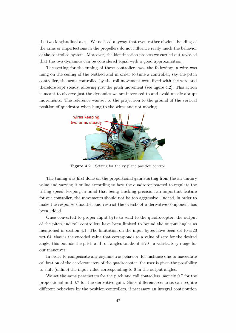
The setting for the tuning of these controllers was the following: a wire washung on the ceiling of the testbed and in order to tune a controller, say the pitchcontroller, the arms controlled by the roll movement were fixed with the wire andtherefore kept steady, allowing just the pitch movement (see figure 4.2). This actionis meant to observe just the dynamics we are interested to and avoid unsafe abruptmovements. The reference was set to the projection to the ground of the verticalposition of quadrotor when hung to the wires and not moving.

Figure 4.2 – Setting for the xy plane position control.

The tuning was first done on the proportional gain starting from the an unitaryvalue and varying it online according to how the quadrotor reacted to regulate thetilting speed, keeping in mind that being tracking precision an important featurefor our controller, the movements should not be too aggressive. Indeed, in order tomake the response smoother and restrict the overshoot a derivative component hasbeen added.

Once converted to proper input byte to send to the quadrocopter, the outputof the pitch and roll controllers have been limited to bound the output angles asmentioned in section 4.1. The limitation on the input bytes have been set to ±20wrt 64, that is the encoded value that corresponds to a value of zero for the desiredangle; this bounds the pitch and roll angles to about ±20°, a satisfactory range forour maneuver.

In order to compensate any asymmetric behavior, for instance due to inaccuratecalibration of the accelerometers of the quadrocopter, the user is given the possibilityto shift (online) the input value corresponding to 0 in the output angles.

We set the same parameters for the pitch and roll controllers, namely 0.7 for theproportional and 0.7 for the derivative gain. Since different scenarios can requiredifferent behaviors by the position controllers, if necessary an integral contribution

42

(0.05 ÷ 0.1) could be added when a higher overshoot could be allowed for the sake ofspeed and steady precision.

4.2.3 Height controller

The controller of the vertical position is the one that took longer to tune, and alsothe least accurate; its performances are deeply influenced by the battery status. Inorder to tune this controller we placed the quadrocopter on the ground and activateall the other (already tuned) controllers. A step was given to the throttle in order forthe vehicle to become airborne and the proportional and derivative gains were tunedto keep it as steady as possible in the air, paying attention to immediately decreaseand eventually cut the throttle with the manual control if the quadrocopter seemedto raise too fast in the air and going out of control. After obtaining reasonablyreduced oscillations, an integral term was added to eliminate the steady state error.A higher value of the integral part produces an overshoot but speeds up the response.

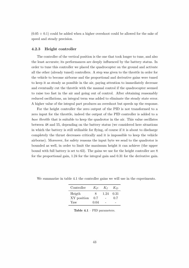
For the height controller the zero output of the PID is not transformed to azero input for the throttle, indeed the output of the PID controller is added to abase throttle that is suitable to keep the quadrotor in the air. This value oscillatesbetween 48 and 55, depending on the battery status (we considered here situationsin which the battery is still utilizable for flying, of course if it is about to dischargecompletely the thrust decreases critically and it is impossible to keep the vehicleairborne). Moreover, for safety reasons the input byte we send to the quadrotor isbounded as well, in order to limit the maximum height it can achieve (the upperbound with full battery is set to 63). The gains we use for the height controller are 8for the proportional gain, 1.24 for the integral gain and 0.31 for the derivative gain.

We summarize in table 4.1 the controller gains we will use in the experiments.

Controller KP KI KD

Heigth 8 1.24 0.31XY position 0.7 - 0.7Yaw 0.04 - -

Table 4.1 – PID parameters.

43

4.3 Experimental results

In this section we report the results of the test-bed implementation of differentkinds of scenarios.

4.3.1 Hover

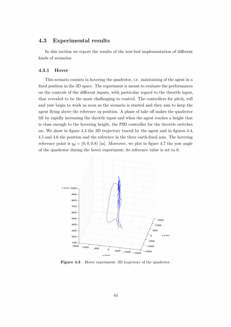
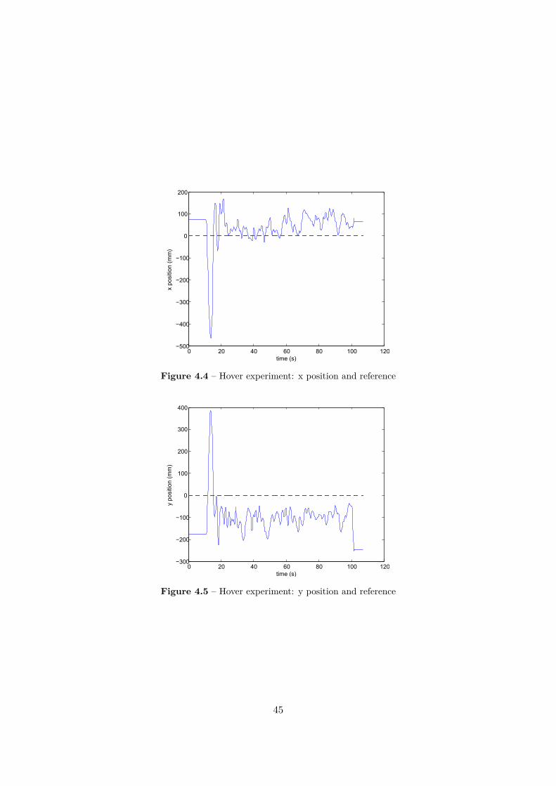
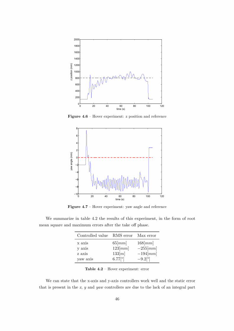
This scenario consists in hovering the quadrotor, i.e. maintaining of the agent in afixed position in the 3D space. The experiment is meant to evaluate the performanceson the controls of the different inputs, with particular regard to the throttle input,that revealed to be the most challenging to control. The controllers for pitch, rolland yaw begin to work as soon as the scenario is started and they aim to keep theagent flying above the reference xy position. A phase of take off makes the quadrotorlift by rapidly increasing the throttle input and when the agent reaches a height thatis close enough to the hovering height, the PID controller for the throttle switcheson. We show in figure 4.3 the 3D trajectory traced by the agent and in figures 4.4,4.5 and 4.6 the position and the reference in the three earth-fixed axis. The hoveringreference point is qd = (0, 0, 0.8) [m]. Moreover, we plot in figure 4.7 the yaw angleof the quadrotor during the hover experiment; its reference value is set to 0.

−1500

−1000

−500

0

500

1000

1500

−1500−1000−5000500

10001500

100

200

300

400

500

600

700

800

900

1000

x (mm)

y (mm)

z (mm)

Figure 4.3 – Hover experiment: 3D trajectory of the quadrotor.

44

0 20 40 60 80 100 120−500

−400

−300

−200

−100

0

100

200

time (s)

x po

sitio

n (m

m)

Figure 4.4 – Hover experiment: x position and reference

0 20 40 60 80 100 120−300

−200

−100

0

100

200

300

400

time (s)

y po

sitio

n (m

m)

Figure 4.5 – Hover experiment: y position and reference

45

0 20 40 60 80 100 1200

200

400

600

800

1000

1200

1400

1600

1800

2000

time (s)

z po

sitio

n (m

m)

Figure 4.6 – Hover experiment: z position and reference

0 20 40 60 80 100 120−10

−8

−6

−4

−2

0

2

4

6

8

time (s)

yaw

ang

le (

mm

)

Figure 4.7 – Hover experiment: yaw angle and reference

We summarize in table 4.2 the results of this experiment, in the form of rootmean square and maximum errors after the take off phase.

Controlled value RMS error Max error

x axis 65[mm] 168[mm]y axis 123[mm] −255[mm]z axis 133[m] −194[mm]yaw axis 6.77[°] −9.2[°]

Table 4.2 – Hover experiment: error

We can state that the x-axis and y-axis controllers work well and the static errorthat is present in the x, y and yaw controllers are due to the lack of an integral part

46

in the corresponding controllers. Since this static error has a value that does notexceed the 10[cm] for the x and y controllers and is about 7[°] for the yaw controller,it is satisfactory: adding an integral part slows down quite a lot the performances, inparticular wrt the x and y controllers. The z position is the most difficult to control,since the input range of the throttle does not permit very smooth variations of thespeed of the motors. This can be fixed in a future implementation by increasing thequantization of the throttle range. Anyway, after a settling time of 10÷ 15[s], theoscillations of the height around its reference does not exceed ±20[cm] and for ourpurposes this value is acceptable, since for the obstacle avoidance we will considerlarger safety radii. The transition between the takeoff phase and the controlled phasecan be made smoother if we provide that the gap between the last value of thethrottle during the takeoff and the base throttle of the height controller is null orsufficiently small.

For this experiment and for each of the next ones, two videos have been recorded:

• The fist one is a top view from a point near the ceiling of the laboratory,recorded by a Logitech HD Webcam C310.

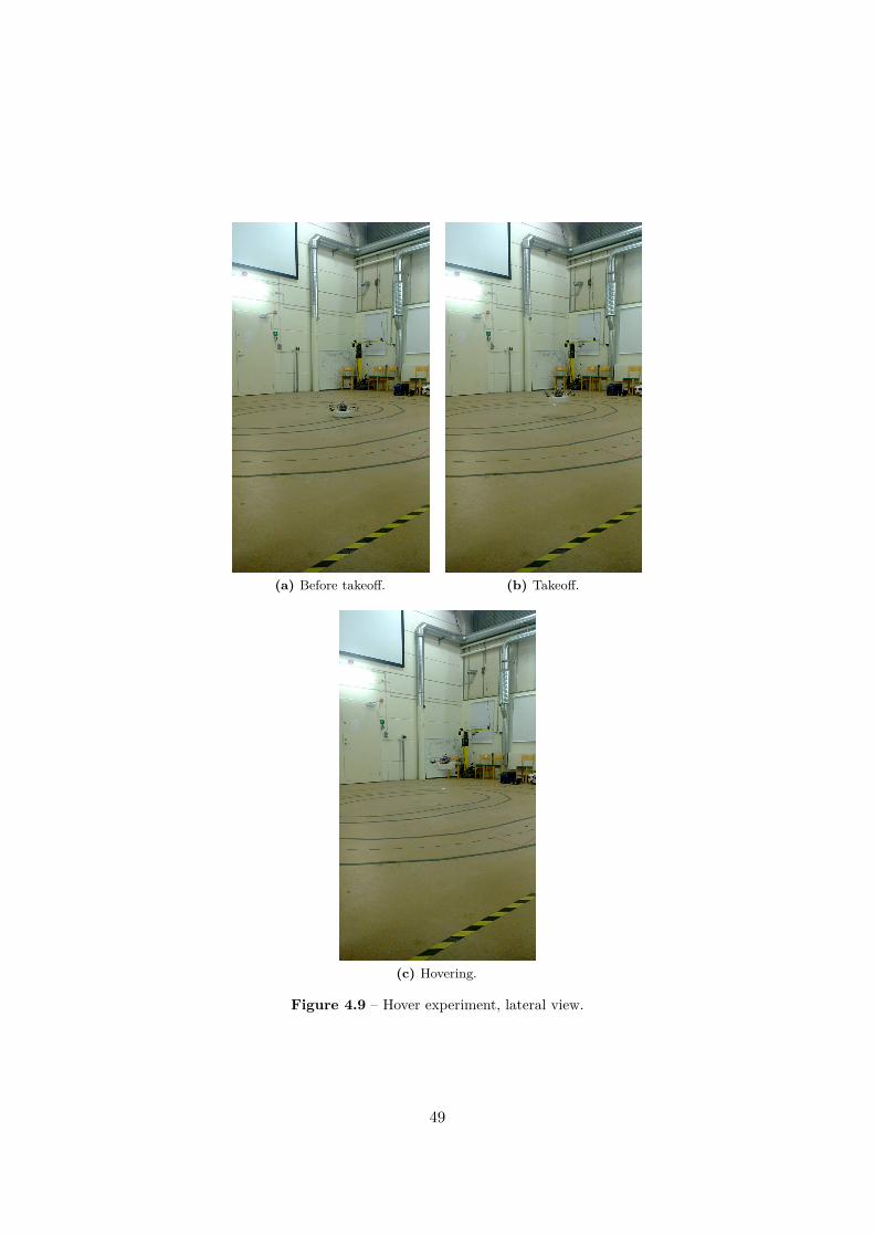
• The second one is a lateral view recorded by the camera of a Nokia Lumia 820smartphone.

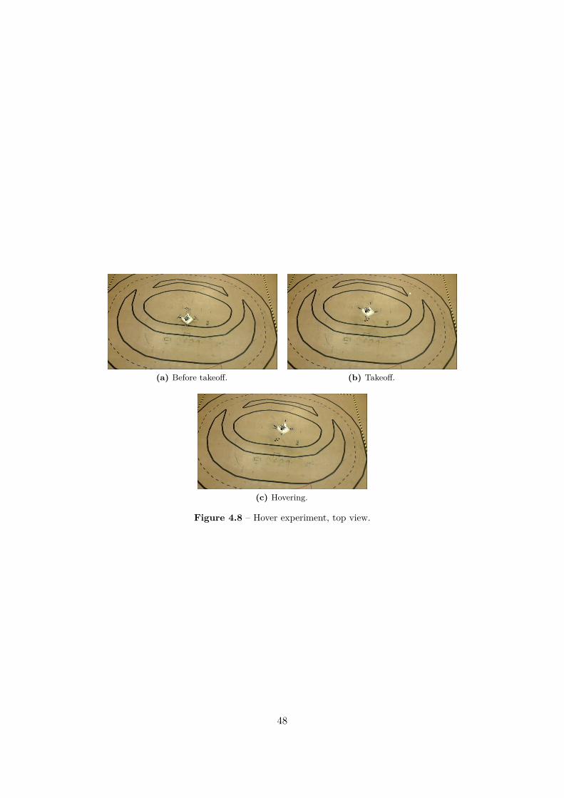
Snapshots of the videos captured for this experiment are reported in figures 4.8and 4.9.

47

(a) Before takeoff. (b) Takeoff.

(c) Hovering.

Figure 4.8 – Hover experiment, top view.

48

(a) Before takeoff. (b) Takeoff.

(c) Hovering.

Figure 4.9 – Hover experiment, lateral view.

49

4.3.2 Circular path

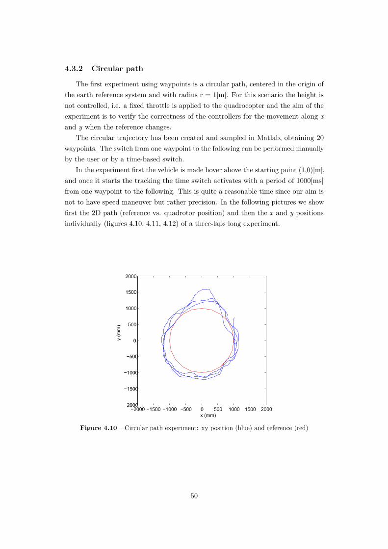
The first experiment using waypoints is a circular path, centered in the origin ofthe earth reference system and with radius r = 1[m]. For this scenario the height isnot controlled, i.e. a fixed throttle is applied to the quadrocopter and the aim of theexperiment is to verify the correctness of the controllers for the movement along xand y when the reference changes.

The circular trajectory has been created and sampled in Matlab, obtaining 20waypoints. The switch from one waypoint to the following can be performed manuallyby the user or by a time-based switch.

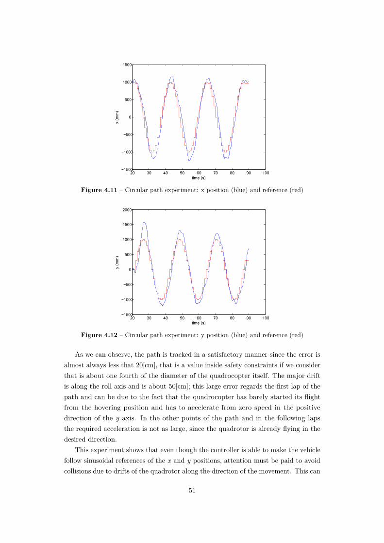
In the experiment first the vehicle is made hover above the starting point (1,0)[m],and once it starts the tracking the time switch activates with a period of 1000[ms]from one waypoint to the following. This is quite a reasonable time since our aim isnot to have speed maneuver but rather precision. In the following pictures we showfirst the 2D path (reference vs. quadrotor position) and then the x and y positionsindividually (figures 4.10, 4.11, 4.12) of a three-laps long experiment.

−2000 −1500 −1000 −500 0 500 1000 1500 2000−2000

−1500

−1000

−500

0

500

1000

1500

2000

x (mm)

y (

mm

)

Figure 4.10 – Circular path experiment: xy position (blue) and reference (red)

50

20 30 40 50 60 70 80 90 100−1500

−1000

−500

0

500

1000

1500

time (s)

x (m

m)

Figure 4.11 – Circular path experiment: x position (blue) and reference (red)

20 30 40 50 60 70 80 90 100−1500

−1000

−500

0

500

1000

1500

2000

time (s)

y (m

m)

Figure 4.12 – Circular path experiment: y position (blue) and reference (red)

As we can observe, the path is tracked in a satisfactory manner since the error isalmost always less that 20[cm], that is a value inside safety constraints if we considerthat is about one fourth of the diameter of the quadrocopter itself. The major driftis along the roll axis and is about 50[cm]; this large error regards the first lap of thepath and can be due to the fact that the quadrocopter has barely started its flightfrom the hovering position and has to accelerate from zero speed in the positivedirection of the y axis. In the other points of the path and in the following lapsthe required acceleration is not as large, since the quadrotor is already flying in thedesired direction.

This experiment shows that even though the controller is able to make the vehiclefollow sinusoidal references of the x and y positions, attention must be paid to avoidcollisions due to drifts of the quadrotor along the direction of the movement. This can

51

be done applying a safety margin on the radii of the obstacles (see next subsection)or the quadrotor itself.

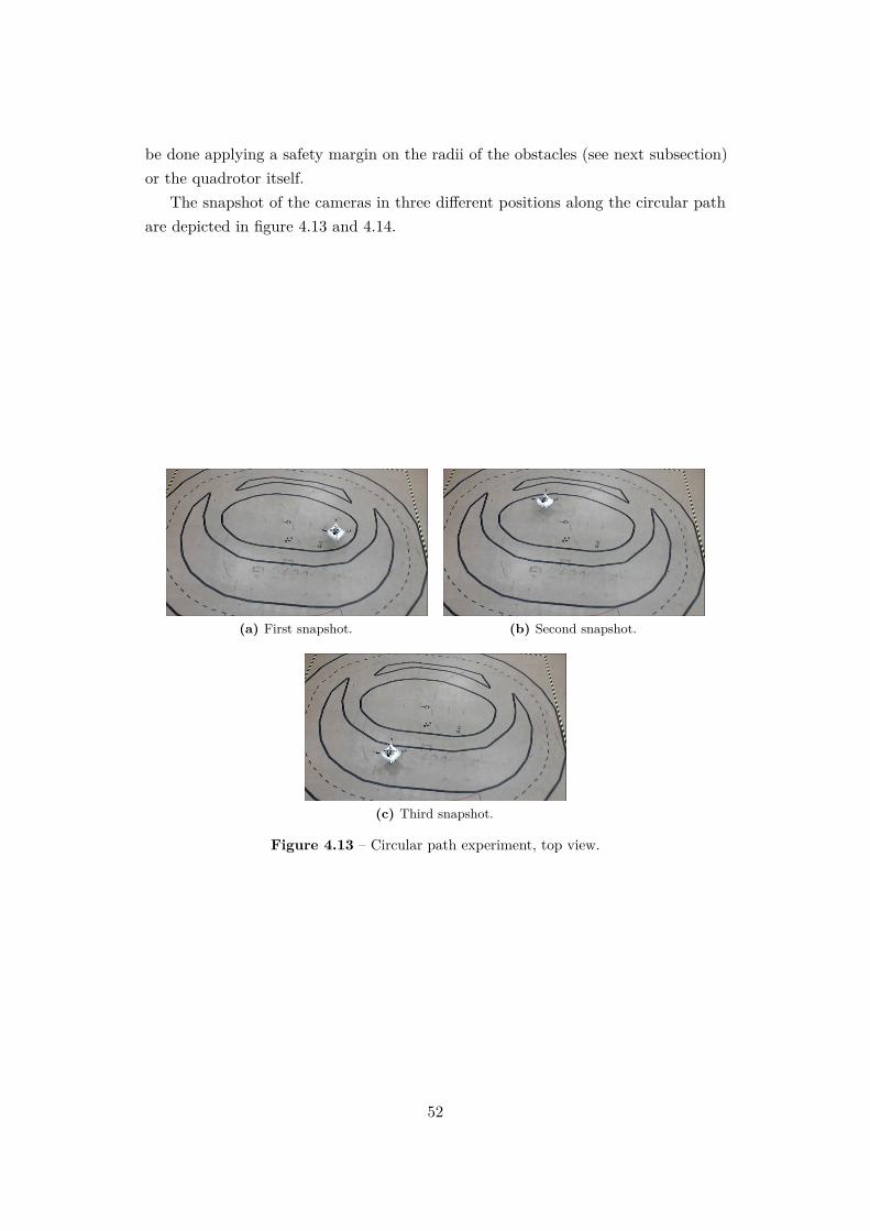
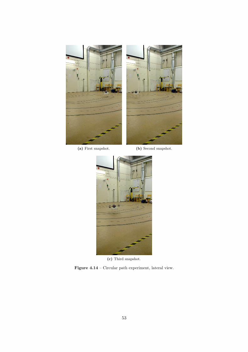
The snapshot of the cameras in three different positions along the circular pathare depicted in figure 4.13 and 4.14.

(a) First snapshot. (b) Second snapshot.

(c) Third snapshot.

Figure 4.13 – Circular path experiment, top view.

52

(a) First snapshot. (b) Second snapshot.

(c) Third snapshot.

Figure 4.14 – Circular path experiment, lateral view.

53

4.3.3 Obstacle avoidance path tracking

The main object of our control is collision-free navigation. The procedure weused in order to get a collision-free path exploits navigation functions to get thesequential positions that should be tracked. We shall summarize in the followinglines the notion of navigation function and its utilization in autonomous navigation.

4.3.3.1 Navigation functions and their application to autonomous navi-gation

Once called En an n-dimensional Euclidean space, q the center of the position ofthe agent and qd its destination, let us define a navigation function as follows:

Definition (Koditscheck and Rimon [29]) Let F ⊂ En be a compact connectedanalytic manifold with boundary. A map Φ : F → [0, 1], is a navigation function ifit is:

1. Analytic on F ;

2. Polar on F , with minimum at qd ∈ F ;

3. Morse on F , i.e. all its critical points are non-degenerate

4. Admissible on F , i.e. limq→∂F

Φ(q) = 1.

Given the radius of the agent r, the destination qd, the positions and radii of theM obstacles qj and ρj , the center and radius of the circular workspace q0 and ρ0, asuitable navigation function is the one expressed as follows.

Let us defineγd(q) , ||q − qd||2

andγ(q) , γd(q)k,

with k ∈ N tuning parameter. γ(q) is a measure of how close the agent is to itsdestination.

Letβj , ||q − qj ||2 − (r + ρj)2,

β0 , (ρ0 − r)2 − ||q − q0||2

and

β =M∏j=0

βj .

54

βj and β0 are indicators of how far the agent is from the obstacles and the workspaceboundary.

A function with the form

Φ =(

γ

γ + β

) 1k

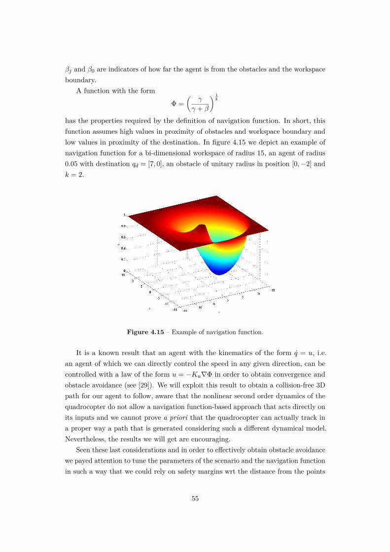
has the properties required by the definition of navigation function. In short, thisfunction assumes high values in proximity of obstacles and workspace boundary andlow values in proximity of the destination. In figure 4.15 we depict an example ofnavigation function for a bi-dimensional workspace of radius 15, an agent of radius0.05 with destination qd = [7, 0], an obstacle of unitary radius in position [0,−2] andk = 2.

Figure 4.15 – Example of navigation function.

It is a known result that an agent with the kinematics of the form q = u, i.e.an agent of which we can directly control the speed in any given direction, can becontrolled with a law of the form u = −Ku∇Φ in order to obtain convergence andobstacle avoidance (see [29]). We will exploit this result to obtain a collision-free 3Dpath for our agent to follow, aware that the nonlinear second order dynamics of thequadrocopter do not allow a navigation function-based approach that acts directly onits inputs and we cannot prove a priori that the quadrocopter can actually track ina proper way a path that is generated considering such a different dynamical model.Nevertheless, the results we will get are encouraging.

Seen these last considerations and in order to effectively obtain obstacle avoidancewe payed attention to tune the parameters of the scenario and the navigation functionin such a way that we could rely on safety margins wrt the distance from the points

55

of the path to the obstacles. This has been done acting

• on the radius of the agent and the obstacles: the longer the radii, the morereliable the distance constraint that provides collision-free navigation;

• on the gain k of the navigation function: a high value of k implies a path closerto the obstacles, and vice versa.

The procedure we follow for obstacle avoidance navigation in our testbed is thefollowing:

• Get from the motion capture system or manually set the initial position,destination and obstacles position in the workspace.

• Translate this coordinates to a simulated environment in Matlab and get thecollision-free path of a single-integrator omnidirectional agent.

• Take back the obtained path to the workspace coordinate system

• Sample the path to get a suitable number of waypoints to track. In the followingexperiments the path has been sampled in such a way that the euclidean distancefrom one waypoint to the following is 20[cm]. This value has been chosen aftersome trials as a trade-off between an easily manageable number of waypointsand a good matching between the continuous5 path computed by Matlab andthe path we get connecting the sampled waypoints.

• Make the quadrocopter hover on the starting point of the path and, when aswitch is commuted, start the tracking of the waypoints. As we said, the switchfrom one waypoint to another can be done manually, basing on a fixed-steptimer but also using a rule on the time the agent stays in a neighborhood ofthe current waypoint. Let us report the pseudocode for the last case:

time_on_position = 0for each iteration of the control algorithm doc_d ← distance between agent’s position and current waypointif c_d≤ d_neighborhood AND time_on_position>max_time_on_positionthenswitch to next waypointtime_on_position = 0

5 Of course the path computed by Matlab is not literally continuous, but is composed of a numberof points more than one order of magnitude greater than the sampled ones. For instance, weset the Matlab solver to integrate along a 500 time samples interval, so the output path iscomposed by 500 points. The number of waypoints we get for the experiments, on the otherhand, is always below 30.

56

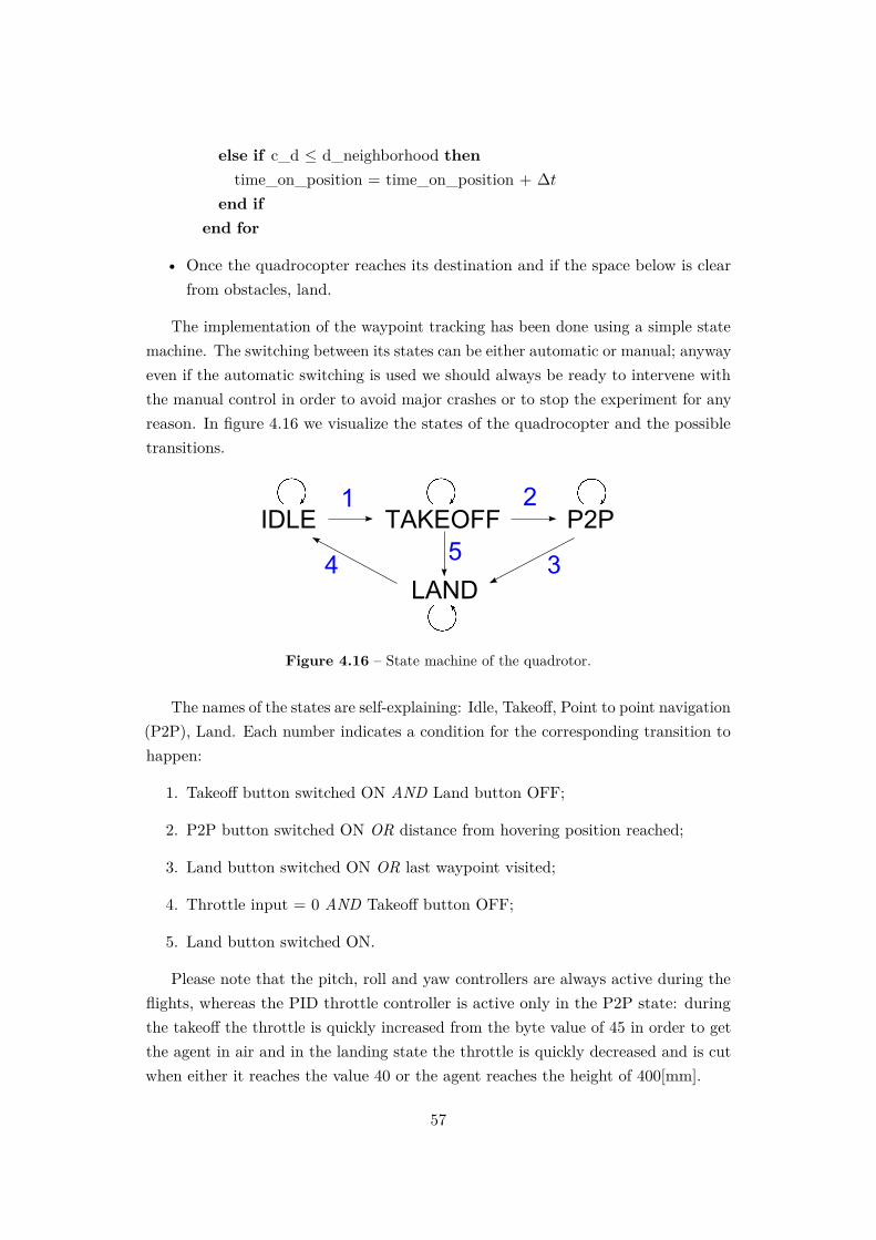
else if c_d ≤ d_neighborhood thentime_on_position = time_on_position + ∆t

end ifend for

• Once the quadrocopter reaches its destination and if the space below is clearfrom obstacles, land.

The implementation of the waypoint tracking has been done using a simple statemachine. The switching between its states can be either automatic or manual; anywayeven if the automatic switching is used we should always be ready to intervene withthe manual control in order to avoid major crashes or to stop the experiment for anyreason. In figure 4.16 we visualize the states of the quadrocopter and the possibletransitions.

IDLE TAKEOFF P2P

LAND

1 2

34 5

Figure 4.16 – State machine of the quadrotor.

The names of the states are self-explaining: Idle, Takeoff, Point to point navigation(P2P), Land. Each number indicates a condition for the corresponding transition tohappen:

1. Takeoff button switched ON AND Land button OFF;

2. P2P button switched ON OR distance from hovering position reached;

3. Land button switched ON OR last waypoint visited;

4. Throttle input = 0 AND Takeoff button OFF;

5. Land button switched ON.

Please note that the pitch, roll and yaw controllers are always active during theflights, whereas the PID throttle controller is active only in the P2P state: duringthe takeoff the throttle is quickly increased from the byte value of 45 in order to getthe agent in air and in the landing state the throttle is quickly decreased and is cutwhen either it reaches the value 40 or the agent reaches the height of 400[mm].

57

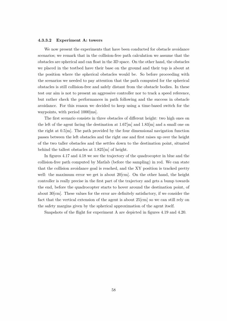
4.3.3.2 Experiment A: towers

We now present the experiments that have been conducted for obstacle avoidancescenarios; we remark that in the collision-free path calculation we assume that theobstacles are spherical and can float in the 3D space. On the other hand, the obstacleswe placed in the testbed have their base on the ground and their top is about atthe position where the spherical obstacles would be. So before proceeding withthe scenarios we needed to pay attention that the path computed for the sphericalobstacles is still collision-free and safely distant from the obstacle bodies. In thesetest our aim is not to present an aggressive controller nor to track a speed reference,but rather check the performances in path following and the success in obstacleavoidance. For this reason we decided to keep using a time-based switch for thewaypoints, with period 1000[ms].

The first scenario consists in three obstacles of different height: two high ones onthe left of the agent facing the destination at 1.67[m] and 1.83[m] and a small one onthe right at 0.5[m]. The path provided by the four dimensional navigation functionpasses between the left obstacles and the right one and first raises up over the heightof the two taller obstacles and the settles down to the destination point, situatedbehind the tallest obstacles at 1.825[m] of height.

In figures 4.17 and 4.18 we see the trajectory of the quadrocopter in blue and thecollision-free path computed by Matlab (before the sampling) in red. We can statethat the collision avoidance goal is reached, and the XY position is tracked prettywell: the maximum error we get is about 20[cm]. On the other hand, the heightcontroller is really precise in the first part of the trajectory and gets a bump towardsthe end, before the quadrocopter starts to hover around the destination point, ofabout 30[cm]. These values for the error are definitely satisfactory, if we consider thefact that the vertical extension of the agent is about 25[cm] so we can still rely onthe safety margins given by the spherical approximation of the agent itself.

Snapshots of the flight for experiment A are depicted in figures 4.19 and 4.20.

58

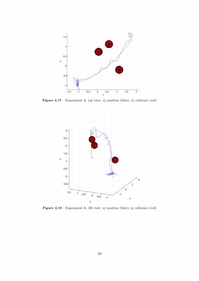
−1.5 −1 −0.5 0 0.5 1 1.5 2

−1

−0.5

0

0.5

1

1.5

x

y

Figure 4.17 – Experiment A, top view: xy position (blue), xy reference (red)

−1

0

1

2

−1−0.500.511.5

−0.5

0

0.5

1

1.5

2

2.5

3

xy

z

Figure 4.18 – Experiment A, 3D view: xy position (blue), xy reference (red)

59

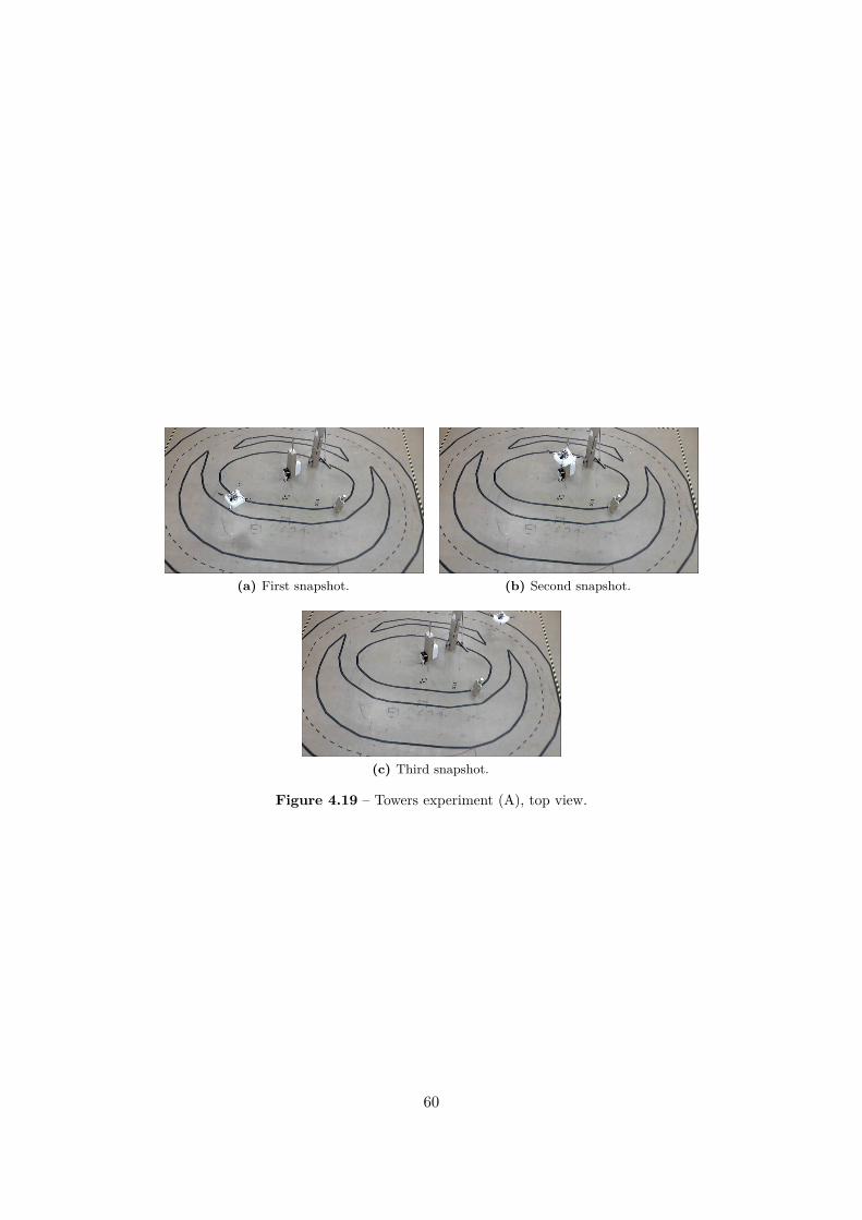
(a) First snapshot. (b) Second snapshot.

(c) Third snapshot.

Figure 4.19 – Towers experiment (A), top view.

60

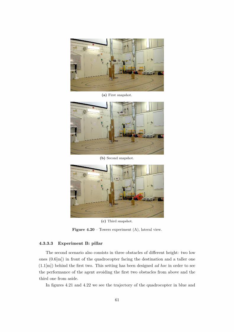
(a) First snapshot.

(b) Second snapshot.

(c) Third snapshot.

Figure 4.20 – Towers experiment (A), lateral view.

4.3.3.3 Experiment B: pillar

The second scenario also consists in three obstacles of different height: two lowones (0.6[m]) in front of the quadrocopter facing the destination and a taller one(1.1[m]) behind the first two. This setting has been designed ad hoc in order to seethe performance of the agent avoiding the first two obstacles from above and thethird one from aside.

In figures 4.21 and 4.22 we see the trajectory of the quadrocopter in blue and

61

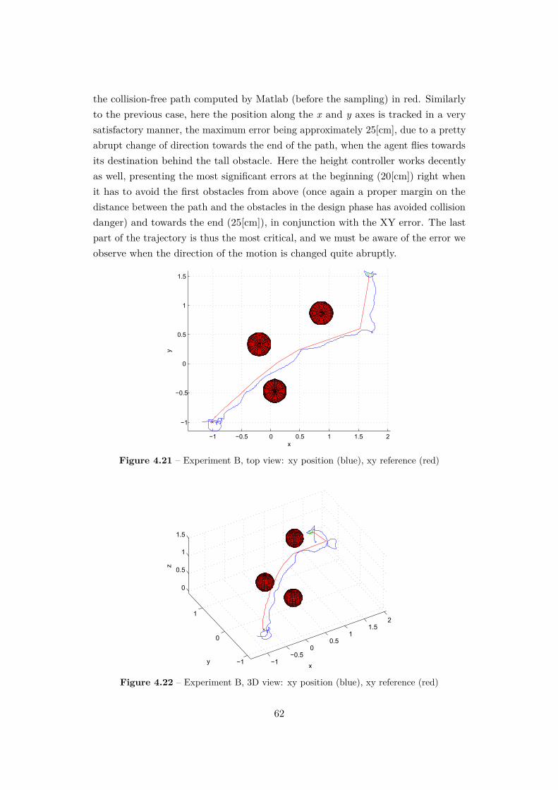
the collision-free path computed by Matlab (before the sampling) in red. Similarlyto the previous case, here the position along the x and y axes is tracked in a verysatisfactory manner, the maximum error being approximately 25[cm], due to a prettyabrupt change of direction towards the end of the path, when the agent flies towardsits destination behind the tall obstacle. Here the height controller works decentlyas well, presenting the most significant errors at the beginning (20[cm]) right whenit has to avoid the first obstacles from above (once again a proper margin on thedistance between the path and the obstacles in the design phase has avoided collisiondanger) and towards the end (25[cm]), in conjunction with the XY error. The lastpart of the trajectory is thus the most critical, and we must be aware of the error weobserve when the direction of the motion is changed quite abruptly.

−1 −0.5 0 0.5 1 1.5 2

−1

−0.5

0

0.5

1

1.5

x

y

Figure 4.21 – Experiment B, top view: xy position (blue), xy reference (red)

−1−0.5

00.5

11.5

2

−1

0

1

0

0.5

1

1.5

xy

z

Figure 4.22 – Experiment B, 3D view: xy position (blue), xy reference (red)

62

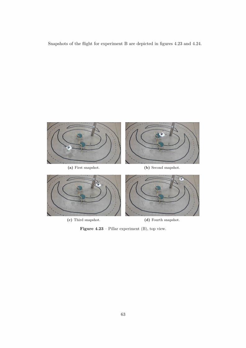
Snapshots of the flight for experiment B are depicted in figures 4.23 and 4.24.

(a) First snapshot. (b) Second snapshot.

(c) Third snapshot. (d) Fourth snapshot.

Figure 4.23 – Pillar experiment (B), top view.

63

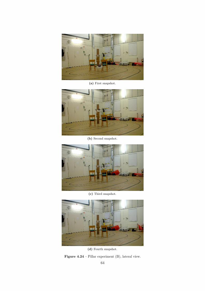
(a) First snapshot.

(b) Second snapshot.

(c) Third snapshot.

(d) Fourth snapshot.

Figure 4.24 – Pillar experiment (B), lateral view.

64

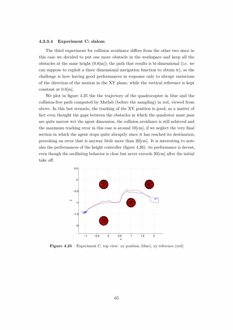
4.3.3.4 Experiment C: slalom

The third experiment for collision avoidance differs from the other two since inthis case we decided to put one more obstacle in the workspace and keep all theobstacles at the same height (0.8[m]); the path that results is bi-dimensional (i.e. wecan suppose to exploit a three dimensional navigation function to obtain it), so thechallenge is here having good performances in response only to abrupt variationsof the direction of the motion in the XY plane, while the vertical reference is keptconstant at 0.8[m].

We plot in figure 4.25 the the trajectory of the quadrocopter in blue and thecollision-free path computed by Matlab (before the sampling) in red, viewed fromabove. In this last scenario, the tracking of the XY position is good, as a matter offact even thought the gaps between the obstacles in which the quadrotor must passare quite narrow wrt the agent dimension, the collision avoidance is still achieved andthe maximum tracking error in this case is around 10[cm], if we neglect the very finalsection in which the agent stops quite abruptly since it has reached its destination,provoking an error that is anyway little more than 20[cm]. It is interesting to notealso the performances of the height controller (figure 4.26): its performance is decent,even though the oscillating behavior is clear but never exceeds 20[cm] after the initialtake off.

−1 −0.5 0 0.5 1 1.5 2

−2

−1.5

−1

−0.5

0

0.5

x

y

Figure 4.25 – Experiment C, top view: xy position (blue), xy reference (red)

65

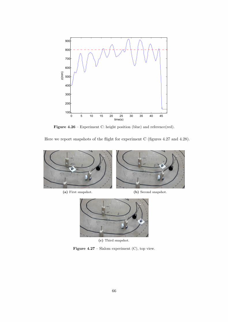
0 5 10 15 20 25 30 35 40 45100

200

300

400

500

600

700

800

900

time(s)

z(mm)

Figure 4.26 – Experiment C: height position (blue) and reference(red).

Here we report snapshots of the flight for experiment C (figures 4.27 and 4.28).

(a) First snapshot. (b) Second snapshot.

(c) Third snapshot.

Figure 4.27 – Slalom experiment (C), top view.

66

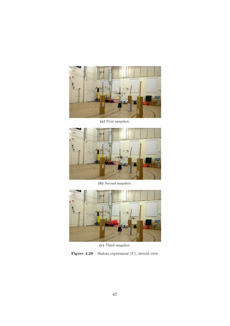
(a) First snapshot.

(b) Second snapshot.

(c) Third snapshot.

Figure 4.28 – Slalom experiment (C), lateral view.

67

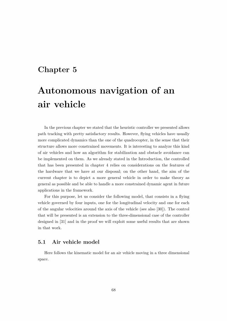
Chapter 5

Autonomous navigation of anair vehicle

In the previous chapter we stated that the heuristic controller we presented allowspath tracking with pretty satisfactory results. However, flying vehicles have usuallymore complicated dynamics than the one of the quadrocopter, in the sense that theirstructure allows more constrained movements. It is interesting to analyze this kindof air vehicles and how an algorithm for stabilization and obstacle avoidance canbe implemented on them. As we already stated in the Introduction, the controlledthat has been presented in chapter 4 relies on considerations on the features ofthe hardware that we have at our disposal; on the other hand, the aim of thecurrent chapter is to depict a more general vehicle in order to make theory asgeneral as possible and be able to handle a more constrained dynamic agent in futureapplications in the framework.

For this purpose, let us consider the following model, that consists in a flyingvehicle governed by four inputs, one for the longitudinal velocity and one for eachof the angular velocities around the axis of the vehicle (see also [30]). The controlthat will be presented is an extension to the three-dimensional case of the controllerdesigned in [31] and in the proof we will exploit some useful results that are shownin that work.

5.1 Air vehicle model

Here follows the kinematic model for an air vehicle moving in a three dimensionalspace.

68

Let q be the state of the agent:

q =

q1

q2

=

x

y

z

φ

θ

ψ

position

orientation

(5.1)

where the orientation is expressed via the Euler angles [ φ θ ψ ]T , that we assumerestricted to the limits φ ∈ (−π, π], θ ∈ (−π

2 ,π2 ], ψ ∈ (−π, π]. Both linear and

angular positions are referred to an Earth-fixed coordinate system.

Let the motion of the agent be described by

q =[q1

q2

], τ =

[τ1

τ2

](5.2)

where τ1 and τ2 define the linear and angular velocities, respectively.

Now we want to express the motion of the vehicle in Body-fixed coordinates. Let

r =

l

a

=

l1

l2

l3

a1

a2

a3

be the vector containing linear and angular positions of the agent in the Body-fixedsystem and let us state that the directions of l1, l2 and l3 are as in figure 5.1.

The corresponding velocities are

v =

v1

v2

=

u

v

w

p

q

r

.

69

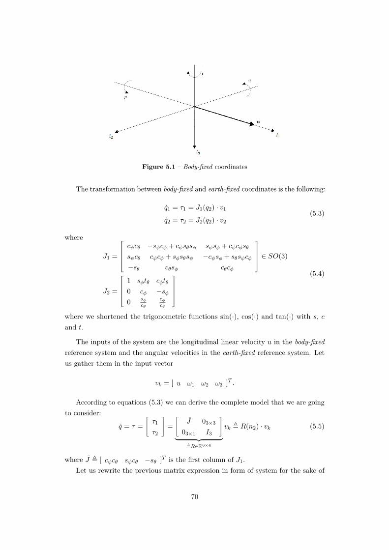
Figure 5.1 – Body-fixed coordinates

The transformation between body-fixed and earth-fixed coordinates is the following:

q1 = τ1 = J1(q2) · v1

q2 = τ2 = J2(q2) · v2(5.3)

where

J1 =

cψcθ −sψcφ + cψsθsφ sψsφ + cψcφsθ

sψcθ cψcφ + sφsθsψ −cψsφ + sθsψcφ

−sθ cθsφ cθcφ

∈ SO(3)

J2 =

1 sφtθ cφtθ

0 cφ −sφ0 sφ

cθ

cφcθ

(5.4)

where we shortened the trigonometric functions sin(·), cos(·) and tan(·) with s, cand t.

The inputs of the system are the longitudinal linear velocity u in the body-fixedreference system and the angular velocities in the earth-fixed reference system. Letus gather them in the input vector

vk = [ u ω1 ω2 ω3 ]T .

According to equations (5.3) we can derive the complete model that we are goingto consider:

q = τ =[τ1

τ2

]=[

J 03×3

03×1 I3

]︸ ︷︷ ︸

,R∈R6×4

vk , R(n2) · vk (5.5)

where J , [ cψcθ sψcθ −sθ ]T is the first column of J1.Let us rewrite the previous matrix expression in form of system for the sake of

70

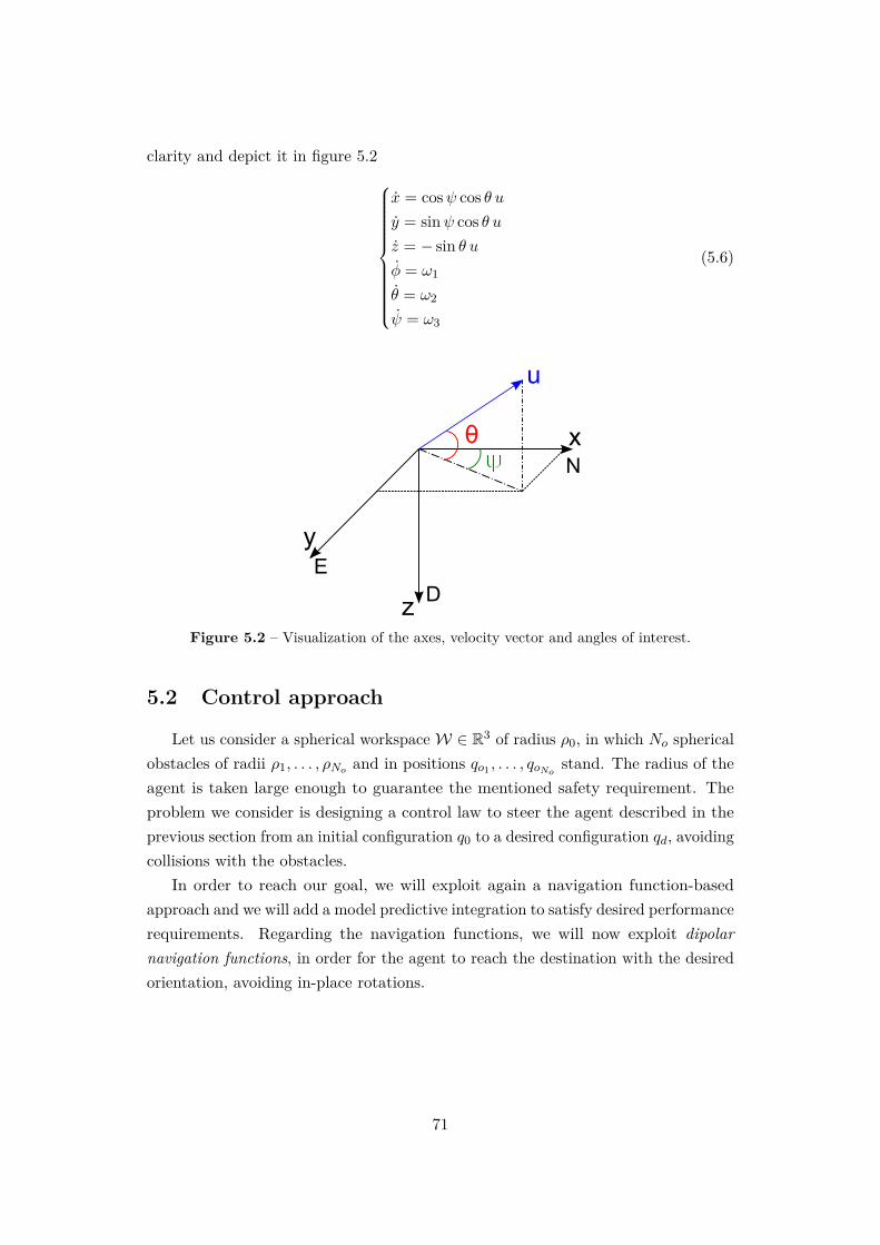
clarity and depict it in figure 5.2

x = cosψ cos θ uy = sinψ cos θ uz = − sin θ uφ = ω1

θ = ω2

ψ = ω3

(5.6)

x

y

z

u

θψ N

ED

Figure 5.2 – Visualization of the axes, velocity vector and angles of interest.

5.2 Control approach

Let us consider a spherical workspace W ∈ R3 of radius ρ0, in which No sphericalobstacles of radii ρ1, . . . , ρNo and in positions qo1 , . . . , qoNo stand. The radius of theagent is taken large enough to guarantee the mentioned safety requirement. Theproblem we consider is designing a control law to steer the agent described in theprevious section from an initial configuration q0 to a desired configuration qd, avoidingcollisions with the obstacles.

In order to reach our goal, we will exploit again a navigation function-basedapproach and we will add a model predictive integration to satisfy desired performancerequirements. Regarding the navigation functions, we will now exploit dipolarnavigation functions, in order for the agent to reach the destination with the desiredorientation, avoiding in-place rotations.

71

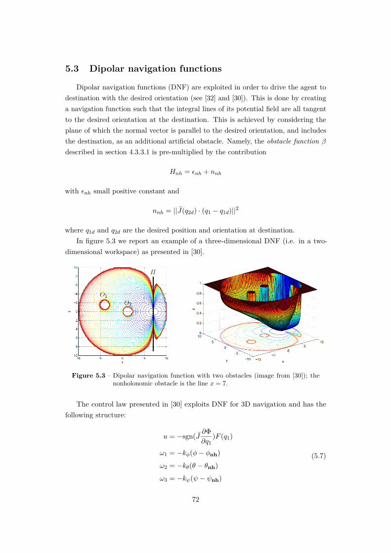
5.3 Dipolar navigation functions

Dipolar navigation functions (DNF) are exploited in order to drive the agent todestination with the desired orientation (see [32] and [30]). This is done by creatinga navigation function such that the integral lines of its potential field are all tangentto the desired orientation at the destination. This is achieved by considering theplane of which the normal vector is parallel to the desired orientation, and includesthe destination, as an additional artificial obstacle. Namely, the obstacle function β

described in section 4.3.3.1 is pre-multiplied by the contribution

Hnh = εnh + nnh

with εnh small positive constant and

nnh = ||J(q2d) · (q1 − q1d)||2

where q1d and q2d are the desired position and orientation at destination.In figure 5.3 we report an example of a three-dimensional DNF (i.e. in a two-

dimensional workspace) as presented in [30].

Figure 5.3 – Dipolar navigation function with two obstacles (image from [30]); thenonholonomic obstacle is the line x = 7.

The control law presented in [30] exploits DNF for 3D navigation and has thefollowing structure:

u = −sgn(J ∂Φ∂q1

)F (q1)

ω1 = −kφ(φ− φnh)

ω2 = −kθ(θ − θnh)

ω3 = −kψ(ψ − ψnh)

(5.7)

72

where Φ is the dipolar navigation function, F is a function that regulates themagnitude of the linear velocity i.e. F = ku|| ∂Φ

∂q1||2 + kz||q1||2, kφ, kθ, kψ, ku, kz are

positive gains and φnh, θnh, ψnh are the nonholonomic angles, described in thefollowing.

Let us define the function

atan2(y, x) , arg(x, y), (x, y) ∈ C

and the partial derivatives

Φx ,∂Φ∂x

Φy ,∂Φ∂y

Φz ,∂Φ∂z

The nonholonomic angles, i.e. the angles defined by the gradient of the dipolarnavigation function, are:

ψnh = atan2 (sign(d)Φy, sign(d)Φx))

θnh = atan2(− sign(d)Φz,

√Φ2x + Φ2

y

)φnh = atan2 (sign(d) cos θ ωψ, sign(d)ωθ)

(5.8)

where the vector sign(d)∇Φ is the direction that the longitudinal axis l1 steers toalign with and the angles ψnh and θnh represent respectively azimuth and elevationof the vector. So according to sign of d the aircraft must approach the target movingforward (i.e. it steers towards the direction of −∇Φ), or backwards (i.e. it steerstoward the direction of ∇Φ).

Since the above-defined angles are not continuous at the destination position(where ∇Φ is null), the approximation scheme in [30] is employed, that guaranteesto have φnh = φd, θnh = θd and ψnh = ψd at the destination.

The bank angle φ does not influence directly the motion of the aircraft and sothe goal of the nonholonomic angle φnh is to track the reference bank angle so thatthe agent tends to eliminate the yaw rate and achieve the required alignment onlythrough pitch rotation.

5.4 Model predictive control

Generally speaking, Model Predictive Control (MPC) consists in an iterativefinite horizon optimization, conducted with regards to a performance measure. Wewould like our agent to reach the destination point and avoid obstacles and at thesame time minimize a functional, that can be related to the control effort, to inputconstraints or other parameters we are interested to keep monitored. Let us call Tp

73

the prediction time horizon; we want to minimize a cost functional in the form:

J(t, x, u, Tp) =∫ (t+Tp)

tΛ(q(τ), u(τ))dτ︸ ︷︷ ︸

Running cost

+ M(q(t+ Tp))︸ ︷︷ ︸Terminal cost

(5.9)

At each calculation time t, the state of the system is sampled and a cost minimizingcontrol law is computed for a time horizon [t, t + Tp). The control law obtainedwith this minimization is applied during a shorter period of time Tc < Tp and theminimization problem is solved again for the new state q(t+ Tc).

The terminal cost M represents an approximation of the cost-to-go from t+Tp →∞: such a function can be well represented by a navigation function Φ (see [31]), sothe cost functional becomes

J(t, x, u, Tp) =∫ (t+Tp)

tΛ(q(τ), u(τ))dτ + Φ(p(t+ Tp)) (5.10)

where we indicate with p the linear position vector of the agent.Now, we want to focus on model predictive navigation, i.e. how MPC can be

applied to the model we are dealing with. In order to do so, let us consider thata control law based only on a navigation function approach does not allow us tochoose one trajectory over another, so we need to introduce some deviations fromthe direction of the DNF gradient in order to have some values we can act on tominimize the index. We define those deviations in terms of variations of the angles θand ψ in respect to the value set by the DNF control (5.7): let us call them δθ andδψ and let us impose that for each prediction interval the deviations are first orderpolynomials (i.e. straight lines) with the previous value of the deviation as startingpoint and the candidate value for the current deviation as ending point1. For eachprediction interval [tk, tk + Tp) the minimization problem to be solved is

J∗(tk, x, Tp) = minδθ([tk, tk + Tp)),δψ([tk, tk + Tp))

J(tk, x, u, Tp)

and the optimal values of the deviations for each prediction interval are the couple

1 We make this assumption in order to keep the value of the deviation bounded during theprediction interval, a requirement that will be exploited in the upcoming demonstration ofstability (see also [31])

74

of deviations that minimize the index when applied together[δθ

δψ

], argmin

δθ([tk, tk + Tp)),δψ([tk, tk + Tp))

J∗(tk, x, Tp)

5.5 Proposed control

The control law that we propose comes from the combination of the input givenby the navigation-function approach and the deviations given by the model predictivecontrol and is the following:

u = − sign(J∂Φ∂q1

)ku

∣∣∣∣∣∣∣∣ ∂Φ∂q1

∣∣∣∣∣∣∣∣2ωφ = −kφ(φ− φnh) + φnh

ωθ = −kθ(θ − θnh − δθ) + θnh + δθ

ωψ = −kψ(ψ − ψnh − δψ) + ψnh + ˙δψ

(5.11)

where:

• Φ is the dipolar navigation function (DNF);• ku, kφ, kθ and kψ are positive constant control parameters;• φnh, θnh and ψnh are the nonholonomic angles;• δθ and δψ are the optimal deviations provided by the model predictive algo-

rithm.

We recall from section 5.4 that the deviations provided by the MP algorithm arecalculated at every prediction interval [t, t+ Tp) and applied during a shorter timeslot called control interval [t, t+Tc). At every control interval the deviations are firstorder polynomials

δθ(τ) = (1− τ

Tc)δθ(t) + ( τ

Tc)δθ(t+ Tc) τ ∈ [t, t+ Tc)

δψ(τ) = (1− τ

Tc)δψ(t) + ( τ

Tc)δψ(t+ Tc) τ ∈ [t, t+ Tc)

and their concatenation is a continuous function by construction.

75

Moreover, the model predictive control is turned off as we reach a neighborhoodof radius rnb of the destination q1d, and we set:

δθ(t ≥ tf ) = ||q1 − q1d||2

rnbδθ(tf )

δψ(t ≥ tf ) = ||q1 − q1d||2

rnbδψ(tf ),

(5.12)

with tf = inft : ||q1 − q1d|| ≤ rnb. These terms are continuous in ||q1 − q1d|| = rnb

and are null with null derivative at the destination point:

δθ(||q1 − q1d|| = rnb) = δθ(tf )

δθ(q1d) = 0

δθ(q1d) = 0

(5.13)

Similar expressions can be found for δψ(t ≥ tf ).

5.5.1 Useful lemmas

We report here two lemmas we are going to use in the demonstration. They havebeen used for demonstrating the two-dimensional case of the problem in [31] andtheir demonstration can be found in the same work.

Lemma 5.5.1 The deviations δθ and δψ are continuous functions and

|δθ| < π

2 , |δψ| < π

2 ∀t

Lemma 5.5.2 At every recalculation time tk, let us modify the sampling set for thedeviations, that originally were Θ = Ψ =

(−π

2 ,π2), as follows:

Θk =(−π2 + |θ(tk)− θnh(tk)− δθ(tk)|,

π

2 − |θ(tk)− θnh(tk)− δθ(tk)|)

Ψk =(−π2 + |ψ(tk)− ψnh(tk)− δψ(tk)|,

π

2 − |ψ(tk)− ψnh(tk)− δψ(tk)|)

By doing so, if at the beginning |θ(0)− θnh(0)| < π2 and |ψ(0)− ψnh(0)| < π

2 , then

|θ(t)− θnh(t)| < π

2 , |ψ(t)− ψnh(t)| < π

2 ∀t

We remark that the hypothesis |θ(0)− θnh(0)| < π2 and |ψ(0)− ψnh(0)| < π

2 arereasonable, in particular if we assume that the agent can perform maneuvering beforetake off.

76

5.5.2 Proof of convergence and collision avoidance

We can finally state the following

Theorem 5.5.3 (Convergence and collision avoidance) An agent described bythe model (5.5) navigating under the control law (5.11) converges to its targetdestination with the desired azimuth and elevation angles, avoiding collisions withobstacles.

Proof Let us consider the ordinate sequence of recalculation times in which the modelpredictive algorithm is applied, tf being the last element: t0, t1, . . . , tk, tk+1, . . . , tf ,with t0 = 0 and tk+1 = tk + Tc.

Now, for each interval [tk, tk+1), tk 6= tf we consider the Lyapunov functioncandidate

Vk = Φ + 12 (θ − θnh − δθ[tk, tk+1))2 + 1

2 (ψ − ψnh − δψ[tk, tk+1))2 (5.14)

and the extended system

xext =

q1

θ

θnh

δθ

ψ

ψnh

δψ

, xext = f(xext) =

Ju

ωθ

θnh

δθ

ωψ

ψnh˙δψ

We can define the Filipov set K[f ](xext) and the generalized derivative of Vk,

∂Vk, as follows:

K[f ] =

JK[u]ωθ

θnh

δθ

ωψ

ψnh˙δψ

, ∂Vk =

∇Φθ − θnh − δθ−(θ − θnh − δθ)−(θ − θnh − δθ)ψ − ψnh − δψ−(ψ − ψnh − δψ)−(ψ − ψnh − δψ)

77

And applying the chain rule we get

˙V =⋂

ξ∈∂Vk

ξT (K[f ](xext, t)) =

=JK[u]∇Φ + ωθ(θ − θnh − δθ)− θnh(θ − θnh − δθ)− δθ(θ − θnh − δθ)+

+ ωψ(ψ − ψnh − δψ)− ψnh(ψ − ψnh − δψ)− ˙δψ(ψ − ψnh − δψ)

Substituting the expressions for ωθ and ωψ (see (5.11)) and defining P , J∇Φ,we obtain

˙Vk = JK[u]∇Φ− kθ(θ − θnh − δθ)2 − kψ(ψ − ψnh − δψ)2 =

= PK[− sign(P )ku ||∇Φ||2

]− kθ(θ − θnh − δθ)2 − kψ(ψ − ψnh − δψ)2 =

= −|P |ku ||∇Φ||2 − kθ(θ − θnh − δθ)2 − kψ(ψ − ψnh − δψ)2

The last two terms of the previous sum are always nonpositive. The first term isthe product of ku ||∇Φ||2 > 0 (we are considering tk 6= tf and ∇Φ is practically nullonly for q1 = q1d since the initial conditions that lead to saddle points are a set ofmeasure zero) and −|P |, that is strictly negative since P is null only if ||∇Φ|| = 0 orif the gradient is normal to the aircraft longitudinal axis2, but this last condition isnot verified as we adjusted the sampling sets following Lemma 1.2.

It is straightforward that Vk−1(tk) = Vk(tk), as a result of Lemma 1.1. So theconcatenation of the Lyapunov function candidates that we considered so far is acontinuous function of time.

Let us consider now the Lyapunov function candidate for t ≥ tf :

Vf = Φ + 12 (θ − θnh − δθ(t ≥ tf ))2 + 1

2 (ψ − ψnh − δψ(t ≥ tf ))2 .

It follows from (5.13) that the concatenation V = V1|V2| . . . |Vf is continuous as well.Moreover, as we write ˙Vf similarly as we did for ˙Vk, we get ˙Vf ≤ 0, because in

this case the first term of the expression can be null.

We now want to apply LaSalle’s principle to V , i.e. we want to exploit the factthat the system converges to the largest invariant subset of S , q| ˙V = 0.

We have that ˙V = 0⇐⇒ ˙Vf = 0, i.e.

−|P |ku ||∇Φ||2 − kθ(θ − θnh − δθ(t ≥ tf ))2 − kψ(ψ − ψnh − δψ(t ≥ tf ))2 = 0

In order for this to hold, the last two terms of the sum must be zero and at leastone of |P | and ||∇Φ|| must be null as well. But actually because of Lemma 1.2 the2 i.e. |θ − θnh| =

π

2 or |ψ − ψnh| =π

2

78

only possibility to get |P | = 0 is that the gradient of the navigation function alsogets null, so for the product to be zero it is necessary and sufficient that ||∇Φ|| iszero. As we already said, the initial conditions leading to saddle points are a set ofmeasure zero, so this practically only happens if q1 = q1d, i.e. at the desired position.

Let us call S1 , q|q1 = q1d the set of configurations in which the agent has thedesired position. If q ∈ S, then

• q1 = q1d, therefore θnh = θd and δθ = 0 (for construction of θnh and δθ), andsimilarly for ψ.

• [(θ − θnh − δθ(t ≥ tf ) = 0) ∧ (ψ − ψnh − δψ(t ≥ tf ) = 0)] implies θ = θd, ψ =ψd

So if q ∈ S, the agent has the desired position and orientation and therefore S is thesingleton qd, that is an invariant set since the components of the input u, ωθ andωψ are null for q = qd.

The convergence to the desired configuration is hence proved.The collision avoidance comes from the properties of the (dipolar) navigation

function. Let us assume no collisions for t = 0: so Φ(t = 0) < 1. Now let us writethe time derivative of Φ:

Φ = ∇Φq1 = ∇ΦJu = P (− sign(P )ku||∇Φ||2) = −|P |ku||∇Φ||2 ≤ 0 ∀t ≥ 0

Therefore Φ(t) < 1, ∀t > 0 and no collisions occur.

79

Chapter 6

Conclusions

In this thesis convergence and obstacle avoidance navigation for an air vehicle hasbeen presented. After a detailed description of the quadrotor platform and the SmartMobility Lab testbed, a general model for quadrotor dynamics has been obtainedand the relations between the control inputs and the behavior of the agent havebeen analyzed through system identification. An heuristic controller for obstacleavoidance has been depicted and the experimental results in the testbed have shownits reliability for our control goals. A more elaborated controller for a general modelof air vehicle has been presented and its properties have been demonstrated, in orderto provide a more general flight scenario, independent from the specific quadrotorsetup, that could be exploited in the testbed in the future.

We wish to give some advice wrt the hardware of the testbed. The arms androtors of the quadrotor were quite fragile and required frequent replacements: toovercome this problem components of more resistant material could be considered.Furthermore, since the height control has been the most challenging and the mostimprecise as well, less powerful motors could be tested on the same quadrotor, inorder for the response to the throttle input to be smoother and for the battery tohave a longer lifetime between charges. For the same reason, a suggestion for futureimplementation is increasing the input quantization.

As far as the control task is concerned, different controllers for waypoint navigation,for instance LQG controllers, could be tested on the same platform and performancescould be compared with the ones of this work. The motion capture system could beintegrated with vision sensors onboard the vehicle in order to provide, for instance,the simulation of inspection or data gathering tasks and IR sensors could be installedin order to improve safety in obstacle avoidance. Nonlinear identification could beperformed on the system to check if more accurate relations can be retrieved and acontrol strategy that exploits explicitly the knowledge of these relations could be

80

studied. The control analyzed in the last chapter or an adaption could be simulatedand implemented in the testbed in the future with air vehicle models fitting thedepicted dynamics. Cooperative navigation between two or more air vehicles couldbe implemented, paying attention for the communication chain to be fast enough toprovide safe control.

81

Bibliography

[1] M. Dempsey, “Eyes of the army – u.s. army roadmap for unmanned aircraftsystems 2010–2035”, 2010. [Online]. Available: http://www-rucker.army.mi

l/usaace/uas/US%20Army%20UAS%20RoadMap%202010%202035.pdf.

[2] K. Fregene, “Unmanned aerial vehicles and control: lockheed martin advancedtechnology laboratories”, Control Systems, IEEE, vol. 32, no. 5, pp. 32–34,2012, issn: 1066-033X. doi: 10.1109/MCS.2012.2205474.

[3] S. Ferrari, M. Anderson, R. Fierro, and W. Lu, “Cooperative navigation forheterogeneous autonomous vehicles via approximate dynamic programming”, inDecision and Control and European Control Conference (CDC-ECC), 2011 50thIEEE Conference on, 2011, pp. 121–127. doi: 10.1109/CDC.2011.6161127.

[4] N. Michael, D. Mellinger, Q. Lindsey, and V. Kumar, “The grasp multiplemicro-uav testbed”, Robotics Automation Magazine, IEEE, vol. 17, no. 3,pp. 56–65, 2010, issn: 1070-9932. doi: 10.1109/MRA.2010.937855.

[5] D. Mellinger, N. Michael, M. Shomin, and V. Kumar, “Recent advances inquadrotor capabilities”, in Robotics and Automation (ICRA), 2011 IEEEInternational Conference on, 2011, pp. 2964–2965. doi: 10.1109/ICRA.2011.

5980163.

[6] P. Bouffard, A. Aswani, and C. Tomlin, “Learning-based model predictivecontrol on a quadrotor: onboard implementation and experimental results”, inRobotics and Automation (ICRA), 2012 IEEE International Conference on,2012, pp. 279–284. doi: 10.1109/ICRA.2012.6225035.

[7] D. Lee, C. Nataraj, T. Burg, and D. Dawson, “Adaptive tracking control of anunderactuated aerial vehicle”, in American Control Conference (ACC), 2011,2011, pp. 2326–2331.

[8] A. Saif, M. Dhaifullah, M. Al-Malki, and M. Shafie, “Modified backsteppingcontrol of quadrotor”, in Systems, Signals and Devices (SSD), 2012 9th Interna-tional Multi-Conference on, 2012, pp. 1–6. doi: 10.1109/SSD.2012.6197975.

82

[9] T. Madani and A. Benallegue, “Backstepping control for a quadrotor helicopter”,in Intelligent Robots and Systems, 2006 IEEE/RSJ International Conferenceon, 2006, pp. 3255–3260. doi: 10.1109/IROS.2006.282433.

[10] M. Khelfi and A. Kacimi, “Robust control with sliding mode for a quadrotorunmanned aerial vehicle”, in Industrial Electronics (ISIE), 2012 IEEE Interna-tional Symposium on, 2012, pp. 886–892. doi: 10.1109/ISIE.2012.6237206.

[11] C.-L. Hwang and C. Jan, “Fuzzy decentralized sliding-mode under-actuatedtrajectory-tracking control for quadrotor unmanned aerial vehicle”, in FuzzySystems (FUZZ-IEEE), 2012 IEEE International Conference on, 2012, pp. 1–10. doi: 10.1109/FUZZ-IEEE.2012.6251290.

[12] A. Roza and M. Maggiore, “Path following controller for a quadrotor helicopter”,in American Control Conference (ACC), 2012, 2012, pp. 4655–4660.

[13] L. Heng, L. Meier, P. Tanskanen, F. Fraundorfer, and M. Pollefeys, “Au-tonomous obstacle avoidance and maneuvering on a vision-guided mav usingon-board processing”, in Robotics and Automation (ICRA), 2011 IEEE Interna-tional Conference on, 2011, pp. 2472–2477. doi: 10.1109/ICRA.2011.5980095.

[14] J. van den Berg, D. Wilkie, S. Guy, M. Niethammer, and D. Manocha, “Lqg-obstacles: feedback control with collision avoidance for mobile robots withmotion and sensing uncertainty”, in Robotics and Automation (ICRA), 2012IEEE International Conference on, 2012, pp. 346–353. doi: 10.1109/ICRA.20

12.6224648.

[15] L. Garcia-Delgado, A. Dzul, V. Santibanez, and M. Llama, “Quad-rotorsformation based on potential functions with obstacle avoidance”, ControlTheory Applications, IET, vol. 6, no. 12, pp. 1787–1802, 2012, issn: 1751-8644.doi: 10.1049/iet-cta.2011.0370.

[16] M. Amoozadeh, Smart mobility lab manual, 1st ed., KTH Stockholm, 2013.[Online]. Available: https://code.google.com/p/kth-smart-mobility-la

b/downloads/list.

[17] C. Anderson et al. (2013). Google code page for the arducopter project, [Online].Available: https://code.google.com/p/arducopter/.

[18] Moteiv corporation, “Tmote sky datasheet”, Data sheet, 2006. [Online]. Avail-able: http://www.eecs.harvard.edu/~konrad/projects/shimmer/refere

nces/tmote-sky-datasheet.pdf.

[19] T. Bresciani, “Modelling, Identification and Control of a Quadrotor Helicopter”,Master’s thesis, Lund University, Sweden, 2008.

83

[20] D. Lee, T. Burg, D. Dawson, D. Shu, B. Xian, and E. Tatlicioglu, “Ro-bust tracking control of an underactuated quadrotor aerial-robot based ona parametric uncertain model”, in Systems, Man and Cybernetics, 2009.SMC 2009. IEEE International Conference on, 2009, pp. 3187–3192. doi:10.1109/ICSMC.2009.5346158.

[21] G. M. Hoffmann, H. Huang, S. L. Waslander, and C. J. Tomlin, “Precision flightcontrol for a multi-vehicle quadrotor helicopter testbed”, Control EngineeringPractice, vol. 19, pp. 1023–1036, 9 2011, issn: 0967-0661. doi: 10.1109/MRA.2

010.937855.

[22] E. Altug, J. Ostrowski, and R. Mahony, “Control of a quadrotor helicopterusing visual feedback”, in Robotics and Automation, 2002. Proceedings. ICRA2002. IEEE International Conference on, vol. 1, 2002, 72–77 vol.1. doi: 10.11

09/ROBOT.2002.1013341.

[23] S. Bouabdallah, “Design and control of quadrotors with application to au-tonomous flying”, PhD thesis, EPFL, 2006.

[24] S. Formentin and M. Lovera, “Flatness-based control of a quadrotor helicoptervia feedforward linearization”, in Decision and Control and European ControlConference (CDC-ECC), 2011 50th IEEE Conference on, 2011, pp. 6171–6176.doi: 10.1109/CDC.2011.6160828.

[25] L. Kis and B. Lantos, “Time-delay extended state estimation and control of aquadrotor helicopter”, in Control Automation (MED), 2012 20th MediterraneanConference on, 2012, pp. 1560–1565. doi: 10.1109/MED.2012.6265861.

[26] T. Lee, M. Leok, and N. McClamroch, “Nonlinear robust tracking control of aquadrotor uav on se(3)”, in American Control Conference (ACC), 2012, 2012,pp. 4649–4654.

[27] D. Mellinger and V. Kumar, “Minimum snap trajectory generation and controlfor quadrotors”, in Robotics and Automation (ICRA), 2011 IEEE InternationalConference on, 2011, pp. 2520–2525. doi: 10.1109/ICRA.2011.5980409.

[28] T. Söderström and P. Stoica, Eds., System identification. Upper Saddle River,NJ, USA: Prentice-Hall, Inc., 1988, isbn: 0-138-81236-5. [Online]. Available:http://user.it.uu.se/~ts/sysidbook.pdf.

[29] D. Koditschek and E. Rimon, “Robot navigation functions on manifolds withboundary”, Advances in Applied Mathematics, vol. 11, no. 4, pp. 412–442, 1990.

84

[30] G. Roussos, D. V. Dimarogonas, and K. J. Kyriakopoulos, “3d navigationand collision avoidance for nonholonomic aircraft-like vehicles”, InternationalJournal of Adaptive Control and Signal Processing, vol. 24, no. 10, pp. 900–920,2010, issn: 1099-1115. doi: 10.1002/acs.1199.

[31] S. Maniatopouloss, “Development of Predictive Navigation Schemes for Aircraft-like Vehicles”, Master’s thesis, National Technical University of Athens, Greece,2012.

[32] H. Tanner, S. Loizou, and K. Kyriakopoulos, “Nonholonomic navigation andcontrol of cooperating mobile manipulators”, Robotics and Automation, IEEETransactions on, vol. 19, no. 1, pp. 53–64, 2003, issn: 1042-296X. doi: 10.110

9/TRA.2002.807549.

85