Embed Size (px)
Citation preview
1
Modelization of a Split in a Ferromagnetic Bodyby an Equivalent Boundary Condition: Part II.
THE INFLUENCE OF SUPER -EXCHANGE AND SURFACE ANISOTROPY .
Kévin Santugini-RepiquetLAGA UMR 7539, Institut Galilée,Université Paris 13, 99 avenue J.B. Clément,
93430 Villetaneuse, France
E-mail: [email protected]
Abstract. We continue the study of equivalent boundary conditions in ferromag-netic domains crossed by a thin split. In this second part, weadd nonhomogenousboundary conditions arising from interactions such as surface anisotropy and super-exchange. We expand the problem up to the first order and establish equivalent bound-ary conditions in presence of surface anisotropy and super-exchange. In particular, thewell-posedness of the expansion problem with equivalent boundary condition and theconvergence in some meaning of the expansion are proven.
Introduction
Following part I [8], we study the behavior of a ferromagnetic domain crossed by a thinsplit. In order to efficiently compute the evolution of the magnetization on such a geometry,we expanded the magnetizationm(0),ε = m(0) + εm(1) on Ωε and derived an equivalentboundary condition on the contact surface:
∂m(1)
∂ν=∂2m(0)
∂ν2.
In this second part of the article, we extend our results whenboundary interactions suchas super-exchange and surface anisotropy are present [4]. The mathematical effect of theseinteractions is to modify the Neumann boundary condition ina nonlinear way. The new termswill be described in section 1. In the same paper, the existence, but not the uniqueness, ofinfinite time weak solutions is also proved.
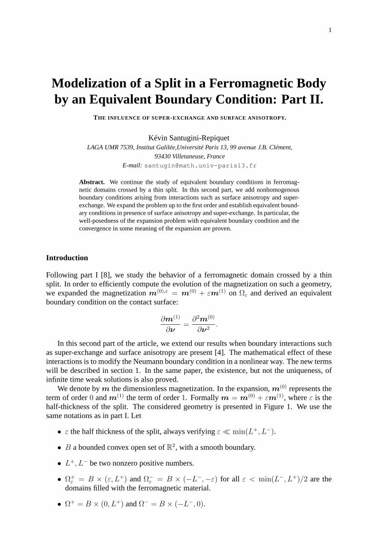
We denote bym the dimensionless magnetization. In the expansion,m(0) represents theterm of order0 andm(1) the term of order1. Formallym = m(0) + εm(1), whereε is thehalf-thickness of the split. The considered geometry is presented in Figure 1. We use thesame notations as in part I. Let
• ε the half thickness of the split, always verifyingε≪ min(L+, L−).
• B a bounded convex open set ofR2, with a smooth boundary.
• L+, L− be two nonzero positive numbers.
• Ω+ε = B × (ε, L+) andΩ−
ε = B × (−L−,−ε) for all ε < min(L−, L+)/2 are thedomains filled with the ferromagnetic material.
• Ω+ = B × (0, L+) andΩ− = B × (−L−, 0).
2 K. Santugini-Repiquet / Modelization of a split in a ferromagnetic body. Part II
z
y
x
Ω+
Ω−
2l
Figure 1: Geometry of the problem
• Ω = Ω+ ∪ Ω− andΩε = Ω+ε ∪ Ω−
ε for all ε < min(L−, L+)/2.
• QεT = Ωε × (0, T ), for all ε < min(L−, L+)/2 andQT = Ω× (0, T ).
• Γ+ε = B×+ε,Γ−
ε = B×−ε andΓ±ε = Γ+
ε ∪Γ−ε . Whenε is omitted, it corresponds
to ε = 0.
• γ0ε is the map that sendsm to its trace onΓ±ε .
• γ0,′ε is the trace map that sendsm to γ0ε (m σ), whereσ is the application that sends(x, y, z, t) to (x, y,−z, t).
• We define the surfaceΓ = B×0. γ0,+ε is the trace map that sendsm to γ00(m τ−ε)on Γ+, whereτ−ε(x, y, z, t) = (x, y, z + ε, t). γ0,−ε is the trace map that sendsm toγ00(m τ+ε) onΓ−.
• γ1ε is the map that sendsm to its normal trace∂m∂ν
onΓ±ε .
• γ1,′ε is the trace map that sendsm to γ1ε (m σ). (x, y, z, t) to (x, y,−z, t).
• γ1,+ε is the trace map that sendsm to γ10(m τ−ε) on Γ+. γ1,−ε is the trace map thatsendsm to γ10(m τε) onΓ−.
• ν represents the unitary exterior normal to the surface boundary of an open set, usuallyΩε orΩ.
In this second part, we use the same notations concerning Sobolev spaces as in section 2.1of [8]. In particular,Hs(Ω) are the classical Sobolev spaces as defined in [1],Hs(Ω) =(Hs(Ω))3, and
Hp,q(Ω× (0, T )) = Hq(0, T ;L2(Ω)) ∩ L2(0, T ;Hp(Ω)). (0.1)
as in Lions-Magenes [5]. We make an extensive use of the spaces H3, 32 (Ω × (0, T )) and
H2,1(Ω× (0, T )). By Lp(Ω), we denote(Lp(Ω))3.In section 1, we describe the super-exchange and surface anisotropy interactions along
with their energies and operators. The description of the other interactions can be found insection 1 of [8]. We also give the complete description of theLandau-Lifshitz system and itslinearization. We also state in this section the well posedness of the Landau-Lifchitz systemwith super-exchange and surface anisotropy as proved in [9]. In section 2, we formally derivethe equivalent boundary condition. In section 3, we give additional inequalities which are not
K. Santugini-Repiquet / Modelization of a split in a ferromagnetic body. Part II 3
contained in section 2.3.1 of [8]. In section 4, we prove the existence of the first orderterm. Then, in section 5, we prove the weakH2,1 convergence of the expansion at first order.Finally, in section 6, we provide the results of some numerical simulations which computethe effect of super-exchange and surface anisotropy to the magnetization terms of both order0 and1.
1 The mathematical model
We only describe the additional material compared to part I section 1. Readers should referto it for more information.
1.1 The surface anisotropy interaction
The surface anisotropy energy, see [4], and the associated operator are
Esa =Ks
2
∫
Γ−ε ∪Γ+
ε
(1− (γ00m · ν)2)dσ(x),
Hsa = Ks((γ00m · ν)ν − γ00m) onΓ−
ε ∪ Γ+ε .
when the ferromagnetic material fillsΩε. This operator has basically the same form as thevolume anisotropy uniaxis operator but withu = ν.
1.2 The super-exchange interaction
This interaction has its roots in quantum mechanics—see [2]. We use the mathematical modelfound in [4]. If the ferromagnetic material fillsΩε, the energy and the operator associated tothe super-exchange operator are
Ese(m) = J1
∫
Γ
(1− γ0ε+m · γ0ε
−m)dσ(x) + J2
∫
Γ
(1− |γ0ε+m · γ0ε
−m|2)dσ(x),
Hse = J1(γ0,′ε m− γ0εm) + 2J2((γ
0εm · γ0,′ε m)γ0,′ε m− |γ0,′ε m|2γ0εm) onΓ− ∪ Γ+.
whereJ1, J2 are positive real numbers. In reality,J1 andJ2 depend on the distanceε, but asthey converge asε tends to0, we will consider them to be constant throughout this article.
1.3 The boundary condition
For the remaining part of the article, we define
Hd,a = Hd +Ha, Hv = Hd +Ha +He, Hs = Hsa +Hse. (1.1)
whereHd,Ha,He are defined in section 1.2 in part I. The boundary conditions onm are
∂m
∂ν= 0 on∂Ωε \ Γ
±ε , (1.2a)
∂m
∂ν=
1
A
(Hs(m)−
(γ00m · Hs(m)
)γ00m
)onΓ+
ε ∪ Γ−ε . (1.2b)
These are obtained as the Euler-Lagrange conditions on the boundary.
4 K. Santugini-Repiquet / Modelization of a split in a ferromagnetic body. Part II
1.4 The Landau-Lifshitz system
The Landau-Lifshitz system is
∂mε
∂t= −mε ×Hv(m
ε)− αmε × (mε ×Hv(mε)) in Ωε × (0, T ), (1.3a)
|mε| = 1 a.e. inΩε × (0, T ), (1.3b)
mε(·, 0) =mε0, (1.3c)
∂mε
∂ν=
0 on∂Ω \ Γ,
Q+(γ00mε, γ0,′0 m
ε) onΓ+ε ,
Q−(γ00mε, γ0,′0 m
ε) onΓ−ε ,
(1.3d)
whereQ±(γ0εm, γ0,′ε m) = Q±r (γ
0εm, γ0,′ε m)− (Q±
r (γ0εm, γ0,′ε m) ·γ0εm)γ0εm withQr being
a polynomial in two variables. It is left to the reader to verify that conditions (1.2) are aparticular case of conditions (1.3d). In [9], we proved the following theorem of existence.
Theorem 1.1. If the initial conditionmε0 belongs toH2(Ωε) and satisfies the boundary con-
dition
∂mε0
∂ν=
0 on∂Ω \ Γ±ε ,
Q+(γ0εmε0, γ
0,′ε m
ε0) onΓ+
ε ,
Q−(γ0εmε0, γ
0,′ε m
ε0) onΓ−
ε ,
(1.4)
and|m0| = 1, then there exists a uniqueT ∗ > 0 andmε in H3, 32 (Ω× (0, T )) for all T < T ∗
satisfying(1.3). The system is well-posed.
Anticipating the expansion of the Landau-Lifshitz system,we introduce a general formof the linearized Landau-Lifshitz system.
∂w
∂t= −m×Hv(w)−w ×Hv(m)− αm× (m×Hv(w))
− αm× (w ×Hv(m))− αw × (m×Hv(m)) + θ onΩ× (0, T ∗),(1.5a)
m ·w = 0, (1.5b)
w(·, 0) = w0. (1.5c)
∂w
∂ν=
0 on∂Ω \ Γ× (0, T ),
DQ+(γ00m, γ0,′0 m) · (γ00w, γ0,′0 w) + β+ onΓ+ × (0, T ),
DQ−(γ00m, γ0,′0 m) · (γ00w, γ0,′0 w) + β− onΓ− × (0, T ).
(1.5d)
wherew is the unknown.β+, β−, θ, w, m are in appropriate functions spaces with valuesin R3. Q+, Q− are the polynomials defined in (1.3d).D is the differentiation operator.
Definition 1.2. We defineH32, 34
00, (Γ× (0, T )) as the subset ofH32, 34 (Γ× (0, T )) containing all
functionsg such that ∫ T
0
∫
Γ
|g(x, t)|2dx
ρ(x)dσ(x)dt < +∞,
whereρ(x) = dist(x, ∂Γ).
This is to ensure compatibility relations, see Lions-Magenes [5]. The existence anduniqueness problem for them(1) are stated by the next two theorems.
K. Santugini-Repiquet / Modelization of a split in a ferromagnetic body. Part II 5
Theorem 1.3. Letm in H3, 32 (Ω × (0, T )) be a solution to the Landau-Lifshitz system with
upper timeT ∗. Letθ be inH1, 12 (Ω × (0, T )) for all T < T ∗ such thatθ is orthogonal tom
almost everywhere. Letβ+, β− in H32, 34
00, (Γ± × (0, T )), orthogonal almost everywhere on theboundaryΓ× (0, T ) tom. Letw0 in H2(Ω) orthogonal almost everywhere inΩ tom, suchthat
∂w0
∂ν= 0 on∂Ω \ Γ,
∂w0
∂ν= DQ+(γ00m0, γ
0,′0 m0)(γ
00w0, γ
0,′0 w0) + β+(·, 0) onΓ+,
∂w0
∂ν= DQ−(γ00w0, γ
0,′0 w0)(γ
00w0, γ
0,′0 w0) + β−(·, 0) onΓ−.
(1.6)
Then, there exists a uniquew in H3, 32 (Ω× (0, T )) solution to system(1.5).
The following theorem solves the existence problem ofm(1). It lowers the requirementsof the previous theorem on the regularity of the data as well as the regularity of the solution.
Theorem 1.4.Letm in H3, 32 (Ω× (0, T )) be a solution to Landau-Lifshitz system with upper
timeT ∗. Let θ be inL2(Ω × (0, T )) for all T < T ∗ such thatθ is orthogonal tom almosteverywhere. Letβ+, β− belonging toH
12, 14 (Γ± × (0, T )), β± ·m = 0. Letw0 in H1(Ω) such
thatm0 ·w0 = 0. Then, there exists a uniquew in H2,1(Ω× (0, T )) solution to system(1.5).
The complete proofs of both theorems can be found at section 4.
Remark1.5. Theorems 1.4 and 1.3 also hold if we replaceΩ byΩε.
2 The equivalent boundary condition
As in the first part, we consider forε small enough an initial conditionmε0 belonging to
H2(Ω), satisfying (1.4) onΓ±ε . We suppose that there existsm(1)
0 such that
‖m(0)0 −m
ε,(0)0 ‖H2(Ωε) = O(1), ‖m
(0)0 −m
ε,(0)0 ‖H1(Ωε) = O(ε), (2.1a)
m(0),ε0 −m
(0)0
ε→ u1
|Ωε0=m
(1)0 weakly inH1(Ωε0) for all ε0 > 0. (2.1b)
We then definemε as the solution to the Landau-Lifshitz system (1.3), with initial conditionmε
0 on Ωε. If we formally expandmε = m(0) + εm(1) up to the first order, we obtain asin [8], equations onm(1) andm(0). Formally,m(0) = m0 and is the solutionm to theLandau-Lifshitz system (1.3) with initial conditionm(0)
0 =m00 on domainΩ. m(1) formally
satisfy
1
ε
∂(mε −m(0))
∂z(·, ·, ε, ·) ≈ −
1
εQ+(γ0ε
+mε, γ0ε
−mε)−Q+(γ00
+
εm(0), γ00
−
εm(0))
−1
εQ+(γ00
+
εm(0), γ00
−
εm(0))−Q+(γ00
+m(0), γ00
−m(0))
−1
ε
∂(γ00+εm
(0) − γ00+m(0))
∂z
≈ −DQ+(γ00+m(0), γ00
−m(0)) ·
(γ00
+m(1) +
∂m(0)
∂z, γ00
−m(1) −
∂m(0)
∂z
)−∂2m(0)
∂ν2.
6 K. Santugini-Repiquet / Modelization of a split in a ferromagnetic body. Part II
Hence, onΓ± the boundary condition is
∂m(1) − ∂m(0)
∂ν
∂ν= DQ±(γ00m
(0), γ0,′0 m(0)) ·
(γ00m
(1) − γ10m(0), γ0,′0 m
(1) − γ1,′0 m(0))
= DQ±(γ00m(0), γ0,′0 m
(0)) · (γ00m(1) − γ10m
(0), γ0,′0 m(1) − γ1,′0 m
(0)). (2.2)
Thus, formallym(1) is the solutionw of the linearized Landau-Lifshitz system (1.5) withm =m(0) and
β+ = −DQ+(γ00m(0), γ0,′0 m
(0)) ·
(∂m(0)
∂ν,∂m(0)
∂ν
)(2.3a)
β− = −DQ±(γ00m(0), γ0,′0 m
(0)) ·
(∂m(0)
∂ν,∂m(0)
∂ν
). (2.3b)
Also, as in part I, formallyθ =m(0)×Hd(γ00m
(0)dσ(Γ))+m(0)×(m(0)×Hd(γ00m
(0)dσ(Γ))).
3 Miscellaneous inequalities and Sobolev spaces
We recall here without proof some well-known properties of Sobolev spaces. It can be ver-ified [8] that the considered domainΩ is regular enough for those inequalities to hold. Inparticular, Sobolev embeddings hold.
Lemma 3.1.The spaceH3, 32 (Ω×(0, T )) is continuously embedded inC0(0, T ; H2(Ω)) and in
L∞(Ω×(0, T )). Besides, the gradient application is linear continuous fromH3, 32 (Ω×(0, T ))
to L4(0, T ;L∞(Ω)).
PROOF: This is a consequence of theorem 4.2 Lions-Magenes [6]. andMaz’ya [7] page274.
Lemma 3.2. H3, 32 (Ω× (0, T )) is an algebra for the pointwise multiplication. Moreover, the
pointwise multiplication of a function inH3, 32 (Ω× (0, T )) and a function inH2,1(Ω× (0, T ))
is in H2,1(Ω× (0, T )).
The constants involved depend strongly onT whenT tends to0.
Definition 3.3. We defineHm− 1
2morc (∂Ω) as the subset ofL2(∂Ω) of functions whose restrictions
on∂B × (0, L),B × 0 etB × L are inHm− 12 .
The following regularity properties hold.
Proposition 3.4(Elliptic regularity).
The spacev ∈ H1(Ω) | v ∈ L2(Ω), ∂v
∂ν∈ H
12morc(∂Ω)
is equal toH2(Ω) and there exists
a constantC such that for allv in H2(Ω)
‖v‖H2(Ω) ≤ C
(‖v‖L2(Ω) + ‖v‖L2(Ω) +
∥∥∥∥∂v
∂ν
∥∥∥∥H
12morc(∂Ω)
). (3.1a)
Proposition 3.5.The spacev ∈ H1(Ω),∇v ∈ L2(Ω), ∂v
∂ν∈ H
32morc(∂Ω)
is equal toH3(Ω)
and there exists a constantC such that for allv in H3(Ω)
‖v‖H3(Ω) ≤ C
(‖v‖L2(Ω) + ‖∇v‖L2(Ω) +
∥∥∥∥∂v
∂ν
∥∥∥∥H
32 (∂Ω)
). (3.1b)
K. Santugini-Repiquet / Modelization of a split in a ferromagnetic body. Part II 7
PROOF: This proposition is a trivial consequence of Proposition 2.8 in part I of thisarticle.
Lemma 3.6. If A is a continuous bilinear operator from spacesX, Y into spaceZ thenA isbilinear continuous from the spaces(L∞ ∩ H
12 )(X), (L∞ ∩ H
12 )(Y ) into (L∞ ∩ H
12 )(Z).
PROOF: The proof is left to the reader. It is similar to the proof of Lemma 2.14 in thefirst part [8].
This lemma allows to recover theH12 regularity in time from the Landau-Lifshitz equation
and theH1(0, T ;H1(Ω)) ∩ L2(0, T ;H3(Ω)) regularity of the solution.
4 Proof of the existence theorems
In this section, we prove the existence Theorems 1.3 and 1.4.
4.1 An equivalent problem
We first develop the second term of Landau-Lifshitz equation. This gives us a system equiv-alent to (1.5). This new system includes equations (1.5c), (1.5d), (1.5b), and the followingdeveloped form of Landau-Lifshitz.
∂w
∂t= −Am×w − Aw ×m+ Aαw + Aα|m|w + 2Aα(∇m · ∇w)m
−m×Hd,a(w)−w ×Hd,a(m)− αm× (m×Hd,a(w))
− αm× (w ×Hd,a(m))− αw × (m×Hd,a(m)) + θ.
(4.1)
Lemma 4.1. Letβ+, β−, θ, andw0 satisfy the hypothesis of Theorem 1.3. Ifw in H3, 32 (Ω×
(0, T )) satisfies equations(1.5c), (1.5d)and(4.1), thenw also satisfies the local orthogonal-ity (1.5b). Thus,w is a solution to Theorem 1.3.
PROOF: The time equation is
∂(w ·m)
∂t= αA
((w ·m) + 2|∇m|2(w ·m)
).
Moreover, the boundary condition is
∂(m ·w)
∂ν= 0 on∂Ω \ Γ× (0, T ),
∂(m ·w)
∂ν= −2Q+
r (γ00m, γ0,′0 m)γ00m · γ00w onΓ+ × (0, T ),
∂(m ·w)
∂ν= −2Q−
r (γ00m, γ0,′0 m)γ00m · γ00w onΓ− × (0, T ).
We multiply equation (4.1) byw ·m and integrate overΩ× (0, T ).
[∫
Ω
|w ·m|2dx
]T
0
+ (αA− η)
∫
QT
∣∣∇(w ·m)∣∣2dx ≤
2αA
∫ T
0
‖∇m‖2L∞(Ω)
∫
Ω
|m ·w|2dx+C
η3
∫
QT
|m ·w|2dx.
By Gronwall’s inequality,m ·w = 0.
We need to prove the existence and uniqueness of solutions tothis new system. We basicallyprove the theorem in four steps.
8 K. Santugini-Repiquet / Modelization of a split in a ferromagnetic body. Part II
1. Existence with the homogenous Neumann boundary condition.
2. Extension of the boundary condition, then existence withan affine Neumann boundarycondition.
3. Particular case with an affine Neumann boundary conditionthat allow the construc-tion of a sequencewn+1 satisfying (4.1), (1.5c) and a Neumann boundary conditioninvolvingwn.
∂wn+1
∂ν=
0 on∂Ω \ Γ× (0, T ),
DQ+(γ00m, γ0,′0 m) · (γ00wn, γ0,′0 w
n) + β+ onΓ+ × (0, T ),
DQ−(γ00m, γ0,′0 m) · (γ00wn, γ0,′0 w
n) + β− onΓ− × (0, T ).
(4.2)
4. Convergence of the sequence to the solution by proving thatthe difference betweentwo elements in the sequence tend to0.
4.2 The affine Landau-Lifshitz system
Theorem 4.2. Let 0 < T ∗. For all T < T ∗, let m anda in H3, 32 (Ω × (0, T )) and θ in
H1, 12 (Ω× (0, T )). Letw0 in H2(Ω), ∂w0
∂ν= 0 on∂Ω. Then, there exists a uniquew satisfying
w(·, 0) = w0,∂w0
∂ν= 0 on∂Ω× (0, T ∗), and equation(4.1).
PROOF: We use Galerkin’s method as in 2.24 in the first part [8]. We introduce theorthonormal basew1, . . . , wn, . . . of L2(Ω) made of the eigenvectors of the Laplace operatorwith Neumann boundary conditions. We denote byVn the subspace generated byw1, . . . , wnand byPn the orthogonal projection onVn in L2(Ω). Pn is also an orthogonal projector inH1(Ω) and inu ∈ H2(Ω), ∂u
∂ν= 0. First, we introduce for each contributionp,
Fp,linm(0)(w) = −w ×Hp(m(0))−m(0)×Hp(w)− αw × (m(0)×Hp(m(0)))
− αm(0)× (w ×Hp(m(0)))− αm(0)× (m(0)×Hp(w)).(4.3)
We look forwn in H1(0, T )⊗ Vn such that
∂wn
∂t− αAwn = Pn(−Aw
n ×m− Am×wn + 2αA(∇m · ∇wn)m)
+ αAPn(|∇m|2wn + F a,d,linm
(wn) + θ),(4.4)
wn(·, 0) = Pn(w0) (4.5)
In subsequent estimates,η will be a positive real that can be chosen arbitrarily small.C willbe a generic constant depending only on domainΩ. To make these estimates, we need theinequalities
‖F a,d,linm
(w)‖L2(Ω) ≤ C ′(1 + ‖m‖H1(Ω))‖w‖H1(Ω), (4.6a)
‖∇F a,d,linm
(w)‖L2(Ω) ≤ C ′(1 + ‖m‖H2(Ω))2‖w‖H2(Ω). (4.6b)
We already know from the proof of Theorem 2.24 in part I.thatwn exists over[0, T ∗)and is unique. Besides,wn is bounded inH2,1(Ω × (0, T )). We only need the following
K. Santugini-Repiquet / Modelization of a split in a ferromagnetic body. Part II 9
additional estimate. We multiply (4.4) by2wn and integrate. Since,2wn belongsVn
1
2
d
dt
∫
Ω
|wn|2dx+ αA
∫
Ω
|∇wn|2dx =
A
∫
Ω
(∇wn ×m) · ∇wndx
︸ ︷︷ ︸I
+A
∫
Ω
(wn ×∇m) · ∇wndx
︸ ︷︷ ︸II
+ A
∫
Ω
(∇m×wn) · ∇wndx
︸ ︷︷ ︸III
−2αA
∫
Ω
(∇m ·D2wn)m · ∇wndx
︸ ︷︷ ︸IV
− 2αA
∫
Ω
(D2m · ∇wn)m · ∇wndx
︸ ︷︷ ︸V
−2αA
∫
Ω
(∇m · ∇wn)∇m · ∇wndx
︸ ︷︷ ︸V I
− 2αA
∫
Ω
(D2m · ∇m)wn · ∇wndx
︸ ︷︷ ︸V II
−αA
∫
Ω
|∇m|2∇wn · ∇wndx
︸ ︷︷ ︸V III
−
∫
Ω
∇θ · ∇wndx
︸ ︷︷ ︸IX
−
∫
Ω
∇F a,d,linm
(wn) · ∇wndx
︸ ︷︷ ︸X
(4.7)
We evaluateI =∫Ω(∇wn ×m) · ∇wndx.
|I| ≤ ‖∇wn‖L6(Ω)‖m‖L3(Ω)‖∇wn‖L2(Ω)
≤1
4η‖m‖2L3(Ω)‖w
n‖2H2(Ω) + η‖∇wn‖2L2(Ω).(4.8a)
Then, we estimateII =∫Ω(wn ×∇m) · ∇wndx.
|II| ≤ ‖wn‖L∞(Ω)‖∇m‖L2(Ω)‖∇wn‖L2(Ω)
≤1
4η‖∇m‖2L2(Ω)‖w
n‖2H2(Ω) + η‖∇wn‖2L2(Ω).(4.8b)
EstimatingIII =∫Ω(∇m×wn) · ∇wndx yields
|III| ≤ ‖∇m‖L∞(Ω)‖wn‖L2(Ω)‖∇wn‖L2(Ω)
≤1
4η‖D3m‖2L2(Ω)‖w
n‖2L2(Ω) + η‖∇wn‖2L2(Ω).(4.8c)
Then, we estimateIV =∫Ω(∇m ·D2wn)m · ∇wndx.
|IV | ≤ ‖m‖L∞(Ω)‖∇m‖L∞(Ω)‖D2wn‖L2(Ω)‖∇wn‖L2(Ω)
≤1
4η‖m‖2L∞(Ω)‖∇m‖2L∞(Ω)‖∇w
n‖2L2(Ω) + η‖∇wn‖2L2(Ω).(4.8d)
If we estimateV =∫Ω(D2m · ∇wn)m · ∇wndx, we obtain
|V | ≤ ‖D2m‖L6(Ω)‖∇wn‖L3(Ω)‖∇wn‖L2(Ω)
≤1
4η‖m‖2H3(Ω)‖w
n‖2H2(Ω) + η‖∇wn‖2L2(Ω).(4.8e)
10 K. Santugini-Repiquet / Modelization of a split in a ferromagnetic body. Part II
EstimatingV I =∫Ω(∇m · ∇wn)∇m · ∇wn andV III =
∫Ω|∇m|2∇wn · ∇wndx
yields
|V I|, |V III| ≤1
4η‖∇m‖4L∞(Ω)‖∇w
n‖2L2(Ω) + η‖∇wn‖2L2(Ω). (4.8f)
When we estimateV II =∫Ω(D2m · ∇m)wn · ∇wndx, we obtain
|V II| ≤1
4η‖D2m‖2L3(Ω)‖∇m‖2L6(Ω)‖w
n‖2H2(Ω) + η‖∇wn‖2L2(Ω). (4.8g)
EstimatingIX =∫Ω∇θ · ∇wndx yields
|IX| ≤1
4η‖∇θ‖2L2(Ω) + η‖∇wn‖2L2(Ω). (4.8h)
Eventually, we estimateX =∫Ω∇F a,d,lin
m(wn) · ∇wndx using inequality (4.6).
|X| ≤ ‖∇F a,d,linm
(wn)‖L2(Ω)‖∇wn‖L2(Ω)
≤C
4η(1 + ‖m‖2H2(Ω))‖w
n‖2H2(Ω) + η‖∇wn‖2L2(Ω).
We combine inequalities (4.8).
1
2
d
dt
∫
Ω
|wn|2dx+αA
∫
Ω
|∇wn|2dx ≤C
ηg(t)‖wn‖2H2(Ω)+η‖∇wn‖2L2(Ω)+‖∇θ‖2L2(Ω).
(4.9)whereg belongs toL1(0, T ). Choosingη small enough, we can apply Gronwall’s lemma.
‖wn‖L∞(0,T ;L2(Ω)) ≤ CT , ‖∇wn‖L2((0,T )×Ω) ≤ CT . (4.10)
The previous estimate, the regularity inequalities 3.1 andLemma 3.6 prove that the se-quencewn remains bounded inH3, 3
2 (Ω × (0, T )) for all T < T ∗. Thus, there exists asubsequence such that, for allT < T ∗,wn
k converges weakly tow in H3, 32 (Ω× (0, T )). This
limit satisfies∂w∂ν
= 0,w(·, 0) = w0, and∫∫
QT
∂w
∂tψdxdt = −A
∫
QT
(w ×m+m×wdxdt− αw − 2α(∇m · ∇w)m)ψdxdt
+ αA
∫
QT
(|∇m|2wdxdt+ F a,lin
m(w) + F d,lin
m(w) + θ
)ψ,
for all ψ in C1(0, T ;R3) ⊗⋃∞i=1 Vn. Since this space is dense inL2(Ω × (0, T )), w is a
solution.We now prove the uniqueness. Letw andw′ be solutions to the system (4.1) thenδw =
w′ −w is solution to (4.1) affine termθ = 0 and initial conditionw0 = 0. After multiplyingthis equation byδw and integrating overΩ× (0, T ), we obtain the following estimate.
[∫
Ω
|δw|2dxdt
]T
0
+ (αA− η)
∫∫
QT
|δ∇w|2dxdt
≤ C(η)
∫ T
0
(‖m‖2H1(Ω)‖∇m‖2L∞(Ω))‖δw‖2L2(Ω)dt.
The uniqueness follows from choosingη = αA/2 and Gronwall’s lemma.
K. Santugini-Repiquet / Modelization of a split in a ferromagnetic body. Part II 11
Corollary 4.3. Let T < T ∗. Letm in H3, 32 (Ω × (0, T )) for all T < T ∗. Letβ+, β− be in
H32, 34
00, (Γ × (0, T )). Letw0 in H2(Ω) satisfy equation(1.6) with Q+, Q− = 0. Then, thereexists a uniquew solution to equations(1.5c), (4.1)and (1.5d)withQ+, Q− = 0.
PROOF: β+ andβ− satisfy the compatibility relations of Theorem A.6. Thus, thereexists an extensionv in H3, 3
2 (Ω × (0, T )), such thatv satisfy the boundary conditions ofwin (1.5d) withQ+, Q− = 0. We then define
θ = −∂v
∂t− Am×w − Av ×m+ Aαv + Aα|m|w + 2Aα(∇m · ∇v)m
−m×Hd,a(v)− v ×Hd,a(m)− αm× (m×Hd,a(v)− αm× (v ×Hd,a(m))
− αv × (m×Hd,a(m)) + θ.
θ belongs toH1, 12 (Ω × (0, T )), w0 − v(·, 0) satisfy the Neumann boundary conditions. By
Theorem 4.2, there existsu such thatw = u + v is the solution to our theorem. Sinceu isunique, so isw.
Corollary 4.4. Let 0 < T ∗. Letm in H3, 32 (Ω × (0, T )) for all T < T ∗. Let a be in
H3, 32 (Ω× (0, T )). Letβ+, β− be inH
32, 34
00, (Γ× (0, T )). Letw0 in H2(Ω) satisfying
∂w0
∂ν=
0 on∂Ω \ Γ× (0, T ),
DQ+(γ00m0, γ0,′0 m0) · (γ
00a, γ
0,′0 a) + β+ onΓ+ × (0, T ),
DQ−(γ00m0, γ0,′0 m0) · (γ
00a, γ
0,′0 a) + β− onΓ− × (0, T ).
(4.11)
Then, there exists a uniquew solution to equations(1.5c), (4.1)and
∂w
∂ν=
0 on∂Ω \ Γ× (0, T ),
DQ+(γ00m, γ0,′0 m) · (γ00a, γ0,′0 a) + β+ onΓ+ × (0, T ),
DQ−(γ00m, γ0,′0 m) · (γ00a, γ0,′0 a) + β− onΓ− × (0, T ).
(4.12)
PROOF: DQ+(γ00m, γ0,′0 m) · (γ00a, γ0,′0 a) is in H
32, 34
00, (Γ × (0, T )). The easiest way
to prove it is to construct the extension explicitly. First,we recall thatH3, 32 (Ω × (0, T )) is
an algebra. Givenχ in C∞c (−∞,+∞;R+) such thatχ(z) = 0 if z > 3
4min(L+, L−) and
χ(z) = 1 if z < min(L+,L−)2
. We define
g =
DQ+(m,m σ) · (a,a σ) in Ω+,
DQ−(m,m σ) · (a,a σ) in Ω−,
whereσ is the application that maps(x, y, z, t) to (x, y,−z, t). Then, the functionv thatmaps(x, y, z, t) to
∫ z0χ(s)g(x, y, s, t)ds is inH3, 3
2 (Ω× (0, T )) and has the required proper-ties. We apply corollary 4.3.
We need the following lemma to provide a first element to our converging sequence.
Lemma 4.5. Letm0 in H3, 32 (Ω× (0, T )) such that∂w0
∂ν= 0 on∂Ω \ Γ. Then, there existsa
in H3, 32 such thata(·, 0) = w0 and ∂a
∂ν= 0 on∂Ω \ Γ× (0, T ).
PROOF: All the compatibility relations of Theorem A.6 are satisfied. Soa exists.
12 K. Santugini-Repiquet / Modelization of a split in a ferromagnetic body. Part II
4.3 Existence and convergence of the sequence
Theorem 1.3 is a consequence of Lemma 4.1 and the following result.
Theorem 4.6. Letm in H3, 32 (Ω × (0, T )). Letw0 in H2(Ω) satisfying(1.6). Then, there
exists a uniquew in H3, 32 (Ω× (0, T )) solution to system(4.1), (1.5c), and(1.5d).
PROOF: We definewn by induction. Letw−1 in H3, 32 be thea of Lemma 4.5. Then,
knowingwn, we definewn+1 as the unique solution to equations (4.1), (1.5c), and (4.2).This is possible by corollary (4.4). We need estimates on thesize ofwn. Letv0 be inH2(Ω)such that∂v0
∂νvanishes on∂Ω \ Γ, and is equal toDQ±(γ00m, γ0,′0 m) · (γ00w0, γ
0,′0 w0) onΓ.
The existence of suchv0 is given by the same construction as the one found in the proofofcorollary 4.4. We defineu0 = w0 − v0. We first defineu as theH3, 3
2 (Ω × (0, T )) solutionto equations (1.5c), (4.1) and (1.5d) withQ± = 0, θ = 0, and initial conditionu0, but withsameβ±. Note that ifβ± = 0 thenu = 0. This solution exists by corollary (4.3). We makeall of our estimates onvn = wn − u. vn satisfy (1.5c), (4.1) and (4.2) with same initialcondition,Q±, andθ but β± = DQ±(γ00m, γ0,′0 m) · (γ00u, γ
0,′0 u). These are basically the
same estimates as those of the proof of Theorem 4.2. But, the nonhomogenous Neumannboundary conditions force us to use more complicated forms of inequalities (3.1). Thus, anupper bound on theL2 norm ofv does not yield an upper bound on theH2 norm. Weintroduce our preliminary estimates.
‖vn+1‖2H2(Ω) ≤ C(‖vn+1‖2L2(Ω) + ‖vn+1‖2L2(Ω) + ‖DQ±(γ00m, γ0,′0 m) · (γ00w
n, γ0,′0 wn)‖2
H12 (Γ)
)
But,
‖DQ±(m,m σ) · (wn,wn σ)‖2H
12 (Γ)
≤ P(‖m‖H2(Ω)
)‖vn + u‖2H1(Ω)
Butm is in C([0, T ∗);H2(Ω)). Thus,
sup1≤n≤N
‖vn‖2H2(Ω)
≤ C
(sup
1≤n≤N
‖vn‖2H1(Ω)
+ sup1≤n≤N
‖vn‖2L2(Ω)
+ ‖u‖2H1(Ω) + ‖v0‖2H2(Ω)
) (4.13a)
We do the same estimate for theH3 norm.
‖vn+1‖2H3(Ω) ≤ C(‖vn+1‖2L2(Ω) + ‖∇vn+1‖2L2(Ω)
+ ‖DQ±(γ00m, γ0,′0 m) · (γ00wn, γ0,′0 w
n)‖2H
32 (Γ)
)
But
‖DQ±(m,m σ) · (wn,wn σ)‖2H
32 (Γ)
≤ P(‖m‖H2(Ω)
)‖vn + u‖2H2(Ω)
Thus,
sup1≤n≤N
‖vn‖2H3(Ω)
≤ C
(sup
1≤n≤N
‖vn‖2H1(Ω)
+ sup
1≤n≤N
‖∇vn‖2L2(Ω)
+ ‖u‖2H2(Ω) + ‖v0‖2H3(Ω)
) (4.13b)
With inequalities (4.13), we can make useful estimates. We make three estimates on the normof vn for n ≥ 1.
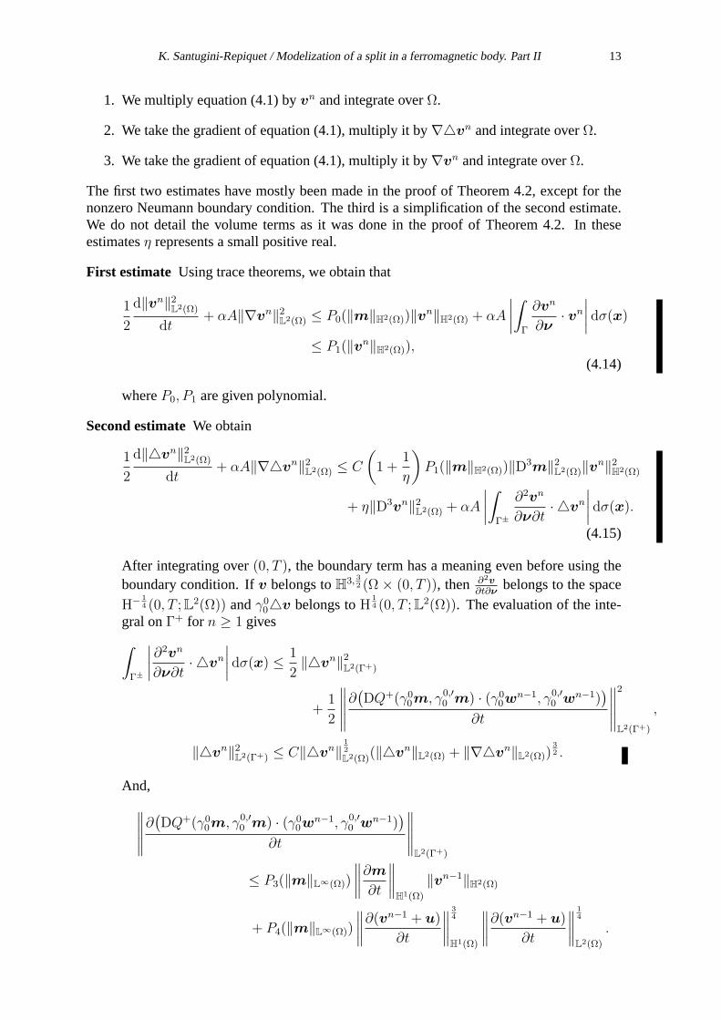
K. Santugini-Repiquet / Modelization of a split in a ferromagnetic body. Part II 13
1. We multiply equation (4.1) byvn and integrate overΩ.
2. We take the gradient of equation (4.1), multiply it by∇vn and integrate overΩ.
3. We take the gradient of equation (4.1), multiply it by∇vn and integrate overΩ.
The first two estimates have mostly been made in the proof of Theorem 4.2, except for thenonzero Neumann boundary condition. The third is a simplification of the second estimate.We do not detail the volume terms as it was done in the proof of Theorem 4.2. In theseestimatesη represents a small positive real.
First estimate Using trace theorems, we obtain that
1
2
d‖vn‖2L2(Ω)
dt+ αA‖∇vn‖2L2(Ω) ≤ P0(‖m‖H2(Ω))‖v
n‖H2(Ω) + αA
∣∣∣∣∫
Γ
∂vn
∂ν· vn∣∣∣∣ dσ(x)
≤ P1(‖vn‖H2(Ω)),
(4.14)
whereP0, P1 are given polynomial.
Second estimateWe obtain
1
2
d‖vn‖2L2(Ω)
dt+ αA‖∇vn‖2L2(Ω) ≤ C
(1 +
1
η
)P1(‖m‖H2(Ω))‖D
3m‖2L2(Ω)‖vn‖2H2(Ω)
+ η‖D3vn‖2L2(Ω) + αA
∣∣∣∣∫
Γ±
∂2vn
∂ν∂t· vn
∣∣∣∣ dσ(x).(4.15)
After integrating over(0, T ), the boundary term has a meaning even before using theboundary condition. Ifv belongs toH3, 3
2 (Ω × (0, T )), then ∂2v∂t∂ν
belongs to the spaceH− 1
4 (0, T ;L2(Ω)) andγ00v belongs toH14 (0, T ;L2(Ω)). The evaluation of the inte-
gral onΓ+ for n ≥ 1 gives
∫
Γ±
∣∣∣∣∂2vn
∂ν∂t· vn
∣∣∣∣ dσ(x) ≤1
2‖vn‖2L2(Γ+)
+1
2
∥∥∥∥∥∂(DQ+(γ00m, γ0,′0 m) · (γ00w
n−1, γ0,′0 wn−1)
)
∂t
∥∥∥∥∥
2
L2(Γ+)
,
‖vn‖2L2(Γ+) ≤ C‖vn‖12
L2(Ω)(‖vn‖L2(Ω) + ‖∇vn‖L2(Ω))
32 .
And,
∥∥∥∥∥∂(DQ+(γ00m, γ0,′0 m) · (γ00w
n−1, γ0,′0 wn−1)
)
∂t
∥∥∥∥∥L2(Γ+)
≤ P3(‖m‖L∞(Ω))
∥∥∥∥∂m
∂t
∥∥∥∥H1(Ω)
‖vn−1‖H2(Ω)
+ P4(‖m‖L∞(Ω))
∥∥∥∥∂(vn−1 + u)
∂t
∥∥∥∥34
H1(Ω)
∥∥∥∥∂(vn−1 + u)
∂t
∥∥∥∥14
L2(Ω)
.
14 K. Santugini-Repiquet / Modelization of a split in a ferromagnetic body. Part II
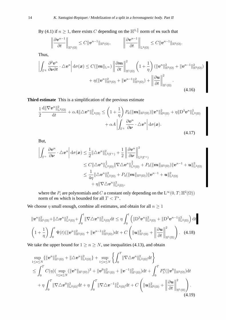
By (4.1) if n ≥ 1, there existsC depending on theH3, 32 norm ofm such that
∥∥∥∥∂vn−1
∂t
∥∥∥∥H1(Ω)
≤ C‖vn−1‖H3(Ω),
∥∥∥∥∂vn−1
∂t
∥∥∥∥L2(Ω)
≤ C‖vn−1‖H2(Ω).
Thus,∣∣∣∣∫
Γ±
∂2vn
∂ν∂t· vn
∣∣∣∣ dσ(x) ≤ C(‖m‖L∞)
∥∥∥∥∂m
∂t
∥∥∥∥2
H1(Ω)
(1 +
1
η
)(‖vn‖2H2(Ω) + ‖vn−1‖2H2(Ω))
+ η(‖vn‖2H3(Ω) + ‖vn−1‖2H3(Ω)) +
∥∥∥∥∂u
∂t
∥∥∥∥2
H1(Ω)
.
(4.16)
Third estimate This is a simplification of the previous estimate
1
2
d‖∇vn‖2L2(Ω)
dt+ αA‖vn‖2L2(Ω) ≤
(1 +
1
η
)P6(‖m‖H2(Ω))‖v
n‖2H2(Ω) + η‖D3vn‖2L2(Ω)
+ αA
∣∣∣∣∫
Γ±
∂vn
∂ν· vn
∣∣∣∣ dσ(x).(4.17)
But,∣∣∣∣∫
Γ+
∂vn
∂ν· vn
∣∣∣∣ dσ(x) ≤1
2‖vn‖2L2(Γ+) +
1
2
∥∥∥∥∂vn
∂ν
∥∥∥∥2
L2(Γ+)
≤ C‖vn‖12
L2(Ω)‖∇vn‖32
L2(Ω) + P3(‖m‖H2(Ω))‖vn−1 + u‖2L2(Ω)
≤1
4η‖vn‖2L2(Ω) + P4(‖m‖H2(Ω))‖v
n−1 + u‖2L2(Ω)
+ η‖∇vn‖2L2(Ω),
where thePi are polynomials andC a constant only depending on theL∞(0, T ;H2(Ω))norm ofm which is bounded for allT < T ∗.
We chooseη small enough, combine all estimates, and obtain for alln ≥ 1
‖vn‖2H1(Ω)+‖vn‖2L2(Ω)+
∫ t
0
‖∇vn‖2L2(Ω)dt ≤ η
∫ t
0
(‖D3vn‖2L2(Ω) + ‖D3vn−1‖2L2(Ω)
)dt
(1 +
1
η
)∫ t
0
Ψ(t)(‖vn‖2H2(Ω) + ‖vn−1‖2H2(Ω))dt+ C
(‖u‖2H1(Ω) +
∥∥∥∥∂u
∂t
∥∥∥∥2
H1(Ω)
). (4.18)
We take the upper bound for1 ≥ n ≥ N , use inequalities (4.13), and obtain
sup1≤n≤N
‖vn‖2H1(Ω) + ‖vn‖2L2(Ω)+ sup1≤n≤N
∫ T
0
‖∇vn‖2L2(Ω)dt
≤
∫ T
0
C(η)( sup1≤n≤N
(‖vn‖H1(Ω))2 + ‖v0‖2H1(Ω) + ‖v−1‖2H1(Ω))dt+
∫ T
0
P η5 (‖v
0‖H2(Ω))dt
+ η
∫ T
0
‖∇v0‖2L2(Ω)dt+ η
∫ T
0
‖∇v−1‖2L2(Ω)dt+ C
(‖u‖2H2(Ω) +
∥∥∥∥∂u
∂t
∥∥∥∥2
H1(Ω)
).
(4.19)
K. Santugini-Repiquet / Modelization of a split in a ferromagnetic body. Part II 15
Reusing inequalities (4.13), we obtain by Gronwall’s lemma that theL∞(0, T ;L2(Ω)) of vn,vn, and∇vn are bounded by a constantC(T ) independent ofn. By inequalities (4.13),there exists a constantCT such that, for allT < T ∗,
‖v‖L∞(0,T ;H2(Ω)) ≤ CT , ‖D3v‖L2(Ω×(0,T )) ≤ CT . (4.20)
Reusing equation (4.1) and Lemma 3.6, we obtain thatvn is bounded inH3, 32 (Ω×(0, T )). We
can extract a subsequence that converge weakly inH3, 32 . We denote byv this limit. Suppose
that1(vnk andvnk+1 both weakly converge inH2,1(Ω× (0, T ))
)=⇒ lim
k→∞vnk = lim
k→∞vnk+1
We extract a further subsequence such thatvnk+1 converges. According to our supposition,the limit isv for both subsequences. OnΓ+,
∂vnk+1
∂ν= DQ+(γ00m, γ0,′0 m) · (γ00v
nk + u, γ0,′0 vnk + u). (4.21)
We take the limit and obtain
∂v
∂ν= DQ+(γ00m, γ0,′0 m) · (γ00v + u, γ0,′0 v + u). (4.22)
Thus,w = v + u is a solution. The corresponding result holds onΓ−. We now proveour previous assumption. For this, we defineδnv = vn+1 − vn, then we can obtain the sameestimate onδnv as obtained in equation (4.18) onv, but withu = 0 and null initial condition.Instead of taking the upper bound, we sum these estimates. The initial conditions of this sumis null. By Gronwall’s inequality, obtain that, for allT < T ∗, there existsCT > 0 such that,for all n ≥ 1,
n∑
k=1
‖δnv‖2L∞(0,T ;H2(Ω)) ≤ CT ,n∑
k=1
‖δnv‖2L2(0,T ;H3(Ω)) ≤ CT .
Thus, our assertion is proved.
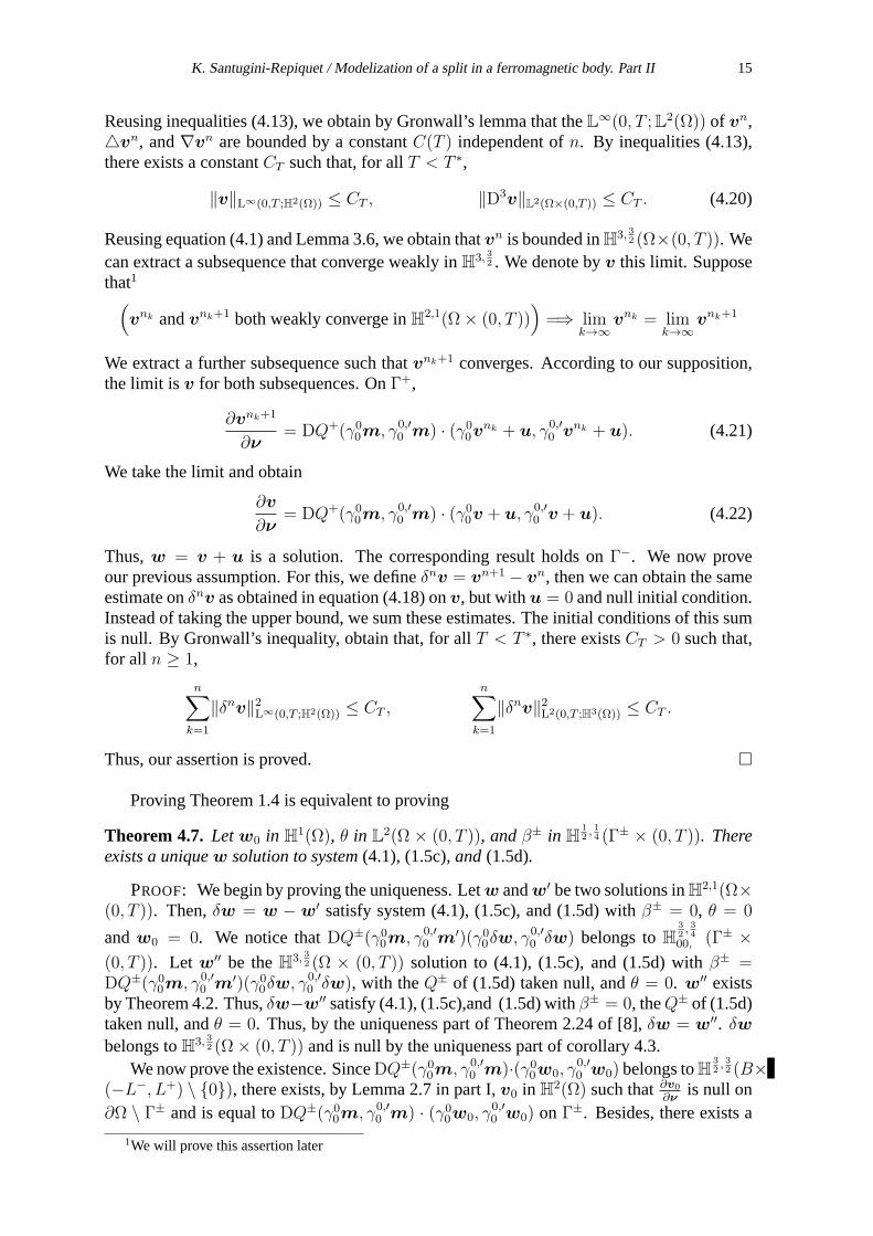
Proving Theorem 1.4 is equivalent to proving
Theorem 4.7. Letw0 in H1(Ω), θ in L2(Ω × (0, T )), andβ± in H12, 14 (Γ± × (0, T )). There
exists a uniquew solution to system(4.1), (1.5c), and(1.5d).
PROOF: We begin by proving the uniqueness. Letw andw′ be two solutions inH2,1(Ω×(0, T )). Then,δw = w − w′ satisfy system (4.1), (1.5c), and (1.5d) withβ± = 0, θ = 0
andw0 = 0. We notice thatDQ±(γ00m, γ0,′0 m′)(γ00δw, γ
0,′0 δw) belongs toH
32, 34
00, (Γ± ×
(0, T )). Let w′′ be theH3, 32 (Ω × (0, T )) solution to (4.1), (1.5c), and (1.5d) withβ± =
DQ±(γ00m, γ0,′0 m′)(γ00δw, γ
0,′0 δw), with theQ± of (1.5d) taken null, andθ = 0. w′′ exists
by Theorem 4.2. Thus,δw−w′′ satisfy (4.1), (1.5c),and (1.5d) withβ± = 0, theQ± of (1.5d)taken null, andθ = 0. Thus, by the uniqueness part of Theorem 2.24 of [8],δw = w′′. δwbelongs toH3, 3
2 (Ω× (0, T )) and is null by the uniqueness part of corollary 4.3.We now prove the existence. SinceDQ±(γ00m, γ0,′0 m)·(γ00w0, γ
0,′0 w0) belongs toH
32, 32 (B×
(−L−, L+) \ 0), there exists, by Lemma 2.7 in part I,v0 in H2(Ω) such that∂v0
∂νis null on
∂Ω \ Γ± and is equal toDQ±(γ00m, γ0,′0 m) · (γ00w0, γ0,′0 w0) onΓ±. Besides, there exists a
1We will prove this assertion later
16 K. Santugini-Repiquet / Modelization of a split in a ferromagnetic body. Part II
constantC independent ofw0 such thatv0 can be chosen so that‖v0‖H2(Ω) ≤ C‖w0‖H1(Ω).We defineu0 asw0−v0. There existsu in H2,1(Ω× (0, T )) that satisfy system (4.1), (1.5c),and (1.5d) with same parameters exceptQ± = 0 and initial conditionu0. This was provedby the author in the first part [8], Theorem 2.24. By Theorem (4.6), there existsv inH3, 3
2 (Ω× (0, T )) with initial conditionv0, sameQ±, β± = dQ±(γ00m, γ0,′0 m) · (γ00u, γ0,′0 u)
belonging toH32, 34
00, andθ = 0. w = v + u is the solution.
5 Convergence
We recall the reader about our problem stated in section 2. Wehave a continuum of solutionsmε to the Landau-Lifshitz system (1.3) on domainΩε with initial conditionsmε
0 satisfyingconditions (2.1). We know by [9] that, for allT < T ∗, theH3, 3
2 (Ωε × (0, T )) norm ofmε0 is
bounded, uniformly inε. The aim of this section is to prove the convergence of the expansionm(0) + εm(1) tomε. We do that in two steps.
1. We derive an upper bound of theH2,1(Ωε × (0, T )) norm of mε−m
(0)
ε.
2. We prove that the weak limit inH2,1(Ω) of mε−m
(0)
εism(1).
We denote by∆Q± the polynomial in four variables such thatQ±(a, b) − Q±(c, d) =∆Q±(a, b, c, d) · (a − c, b − d). Givenm, m′, u0, β+ andβ−, andθ, we consider thefollowing auxiliary system inu.
∂u
∂t− αAu = −Au×m− Am′ ×u+ αA|∇m|2u+ αA((∇m+∇m′) · ∇u)m′
− u×Hd,a(m)−m′ ×Hd,a(u)− αm′ × (m′ ×Hd,a(u))
− αm′ × (u×Hd,a(m))− αu× (m×Hd,a(m)) + θ,(5.1a)
u(·, ·, 0) = u0, (5.1b)
(5.1c)
and the initial condition
∂u
∂ν=
∆Q+(γ00m, γ0,′0 m, γ00m′, γ0,′0 m)(γ00u, γ
0,′0 u) + β+ onB × +ε × (0, T ∗),
∆Q−(γ00m, γ0,′0 m, γ00m′, γ0,′0 m)(γ00u, γ
0,′0 u) + β− onB × −ε × (0, T ∗),
0 on∂Ωε \ (B × ±ε × (0, T ∗)).(5.1d)
First, we state a well-posedness result.
Theorem 5.1. Letm, m′ be inH3, 32 (Ω × (0, T )), let β+, β− be inH
32, 34
00, (Γ × (0, T )), θ in
H1, 12 (Ω× (0, T )), andu0 be inH2(Ω) satisfying
∂u0
∂ν=
∆Q+(γ00m, γ0,′0 m, γ00m′, γ0,′0 m)(γ00u0, γ
0,′0 u0) + β+ onB × +ε,
∆Q−(γ00m, γ0,′0 m, γ00m′, γ0,′0 m)(γ00u0, γ
0,′0 u0) + β− onB × −ε,
0 on∂Ωε \ (B × ±ε).(5.2)
Then, there exists a unique solutionu in H3, 32 (Ω × (0, T )). Furthermore, there exists a
constantC depending on theH3, 32 (Ω× (0, T )) norms ofm,m′ such that
‖u‖H
3, 32 (Ω×(0,T ))≤ C
(‖β±‖
H32 , 3400, (Γ×(0,T ))
+ ‖θ‖H
1, 12 (Ω×(0,T ))+ ‖u0‖H2(Ω)
).
K. Santugini-Repiquet / Modelization of a split in a ferromagnetic body. Part II 17
Besides, suppose thatθ only belongs toL2(Ω × (0, T )), β+, β− only belongs toH12, 14 (Γ ×
(0, T )), andu0 only belongs toH2(Ω). Then, there exists a unique solutionu in H2,1(Ω ×
(0, T )). The problem is also well-posed, there exists a constantC depending on theH3, 32 (Ω×
(0, T )) norms ofm,m′ such that
‖u‖H2,1(Ω×(0,T )) ≤ C(‖β±‖
H12 , 14 (Γ×(0,T ))
+ ‖θ‖L2(Ω×(0,T )) + ‖u0‖H1(Ω)
).
PROOF: We just adapt the proofs of Theorems 4.2, 4.6, and 4.7.
The theorem holds for the domainsΩε, and the constantC(m,m′) while depending on thedomain can be chosen independently ofε for sufficiently smallε.
Proposition 5.2. TheH2,1(Ωε× (0, T )) norm ofmε−m
(0)
εremains bounded for small enough
ε.
PROOF: mε−m
(0)
εis solution to system (5.1) withm = m(0)
|Ωε, m′ = mε, the initial
conditionmε0−m
(0)0
ε, the boundary conditions
β± =1
ε
(γ1εm
(0) − γ10m(0))
+∆Q±(γ00m(0), γ0,′0 m
(0), γ0εm(0), γ0,′ε m
(0)) ·(γ0εm
(0) − γ0,′ε m(0))
ε,
onΓ± × (0, T ) and the affine term
θ =1
εm(0) ×Hd,a(χB×(−ε,+ε)m
(0)) +1
εαm(0) × (m(0) ×Hd,a(χB×(−ε,+ε)m
(0))).
TheH12, 14 (Γ±
ε × (0, T )) norm ofβ±, theL2(Ωε × (0, T )) norm ofθ, and theH1(Ωε) norm ofthe initial condition areO(ε). This latter fact has the same proof as Proposition 3.2 in partI. TheH1(Ωε × (0, T )) norm of the initial condition isO(ε) by hypothesis (2.1). We applyTheorem 5.1.
We now extendmε by reflections onΩ,
mε =
mε onΩε × (0, T ),
3mε(·, ·, 2ε− ·, ·)− 2mε(·, ·, 3ε− 2·, ·) on (B × (−ε, 0))× (0, T ),
3mε(·, ·,−2ε− ·, ·)− 2mε(·, ·,−3ε− 2·, ·) on (B × (0,+ε))× (0, T ).
Then, by the same kind of considerations as those of Lemma 3.4[8], theH2,1(Ω × (0, T ))norm of 1
ε(mε −m(0)) is bounded independently ofε asε tends to0.
Theorem 5.3. The quantitymε,(0))−m
(0)
εconverges weakly tom(1), defined in section 2, in
H2,1(Ω× (0, T )).
PROOF: We extract a decreasing subsequenceεn tending to0 such thatmεn tendsweakly inH2,1(Ω) to m(1). We only need to prove thatm(1) is m(1). Sincem(1) is theunique solution to system (1.5), it is sufficient to prove that m(1) is solution to (1.5) withsame parameters. As in the proof of 3.5 in part I,m(1) satisfy equation (4.1), withθ =
m(0)×Hd(γ00m
(0)dσ(Γ))+m(0)×(m(0)×Hd(γ00m
(0)dσ(Γ))). Besides,m(1)(·, 0) =m(1)0 ,
18 K. Santugini-Repiquet / Modelization of a split in a ferromagnetic body. Part II
see (2.1) for the definition ofm(1)0 , m(1) obviously also verify the homogenous Neumann
boundary condition on∂Ω \ Γ± × (0, T ∗). OnΓ+, we have
∫ T
0
∫
Γ
∣∣∣∣∂(mε −m(0))
∂z(x, ε, t)−
∂(mε −m(0))
∂z(x, 0+, t)
∣∣∣∣2
dσ(x)dt
≤
∫∫ ∣∣∣∣∫ ε
0
∂2(mε −m(0))
∂z2(x, z, t)dz
∣∣∣∣2
dσ(x)dt
≤ ε
∫∫ ∫ ε
0
∣∣∣∣∂2(mε −m(0))
∂z2(x, z, t)
∣∣∣∣2
dzdσ(x)dt ≤ ε3∥∥∥∥mε −m(0)
ε
∥∥∥∥2
H0,2,0
.
Thus, onΓ+, we have
∂m(1)
∂z(·, 0+, ·) = lim
εk→0
1
εk
∂(mεk −m(0))
∂z(·, εk, ·),
= − limεk→0
1
εk
(Q+(γ00m
εk , γ0,′0 mεk)(·, εk, ·)−Q+(γ00m
(0), γ0,′0 m(0))(·, εk, ·)
)
− limεk→0
1
εk
(Q+(γ00m
(0), γ0,′0 m(0))(·, εk, ·)−Q+(γ00m
(0), γ0,′0 m(0))(·, 0+, ·)
)−∂2m(0)
∂z2
= −DQ+(γ00m(0), γ0,′0 m
(0))
(m(1) +
∂m(0)
∂z,m(1) +
∂m(0)
∂z
)−∂2m(0)
∂z2.
Hence,m(1) satisfy (2.2) onΓ+ and by symmetry also onΓ−. Thus,m(1) is them(1) solu-tion of system (1.5) with theβ± of relations (2.3). Sincem(1) is unique, the whole sequenceconverges.
6 Simulations: schemes and numerical results
We use the same schemes as those found in section 4. of [8]. Thecomputation of thediscretized demagnetization field operator is done by the method found in [3]. The onlydifferences are found in the computation of the discretizedexchange operator asm(0) andm(1) satisfy the nonhomogenous Neumann boundary conditions arising from super-exchangeand surface-anisotropy. The discretization of the exchange operator for order0 gives
H0e,h(m)i =
A
h2
∑
j∈V (i)
(mi −mj) +A
h
∑
j∈V C(i)
(Q(mi,mj)) , (6.1)
whereV (i) is the set of all the neighbors of celli in the mesh andV C(i) is the set of allneighbors of celli across the split. We also define the discretization of the theexchangeoperator of order1.
H1e,h(m
0,m1)i =A
h2
∑
j∈V (i)
(m1
i −m1j
)
+ δ(i)A
h2
(m0
N(i) −m0i
h+Q(m0
i ,m0N ′(i)
)
+A
h
∑
j∈V C(i)
DQ(m0i ,m
0j) · (m
1i −Q(mi,mj),m
1j −Q(mj,mi)),
(6.2)
K. Santugini-Repiquet / Modelization of a split in a ferromagnetic body. Part II 19
whereδ(i) is 1 if cell i is adjacent to the interfaceΓ, and0 otherwise. In the former case, cellN(i) is the adjacent cell to celli such that celli is between cellN(i) andΓ. CellN ′(i) beingthe cell such that celli is between cellsN(i) andN ′(i). This discretization requires at leasttwo cells in thez direction on each side of the split.
Our aim in these simulations is to compute equilibrium states. We stop the simulationwhen the derivative of the discrete energy crosses a threshold.
6.0.1 Physical parameters
We use the same physical parametersA,K as in section 4 of [8]. We consider a thin platewith a mesh256×128×1, hence32768 grid points, with a step size of2.3nm. Their magneticparameters are
Ms = 1.4 ∗ 106, A = 10−11/µ0, K = 0.
We also takeKs = 0 — no surface anisotropy — andJ2 = 0. In the geometry considered in
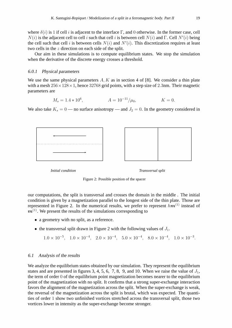
Initial condition Transversal split
Figure 2: Possible position of the spacer
our computations, the split is transversal and crosses the domain in the middle . The initialcondition is given by a magnetization parallel to the longest side of the thin plate. Those arerepresented in Figure 2. In the numerical results, we preferto representhm(1) instead ofm(1). We present the results of the simulations corresponding to
• a geometry with no split, as a reference.
• the transversal split drawn in Figure 2 with the following values ofJ1.
1.0× 10⁻⁵, 1.0× 10⁻⁴, 2.0× 10⁻⁴, 5.0× 10⁻⁴, 8.0× 10⁻⁴, 1.0× 10⁻³.
6.1 Analysis of the results
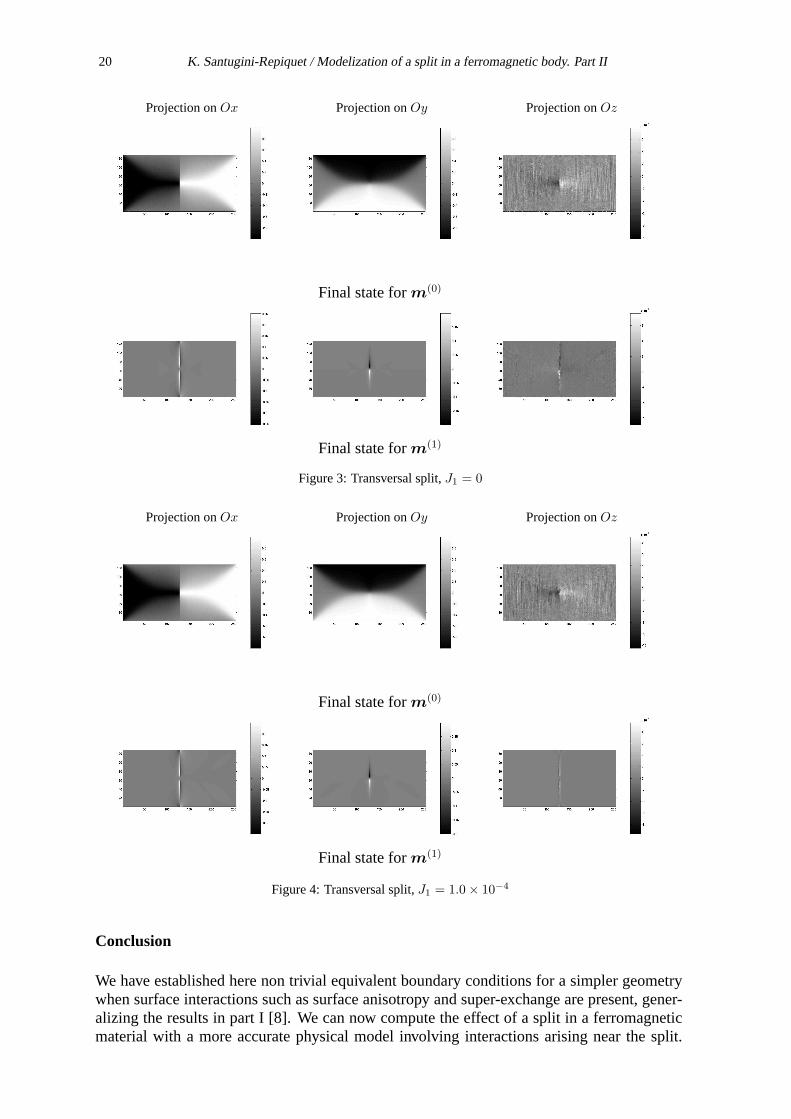
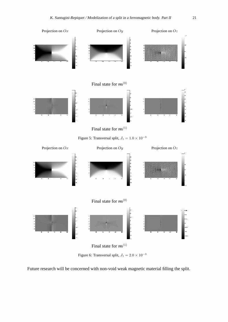
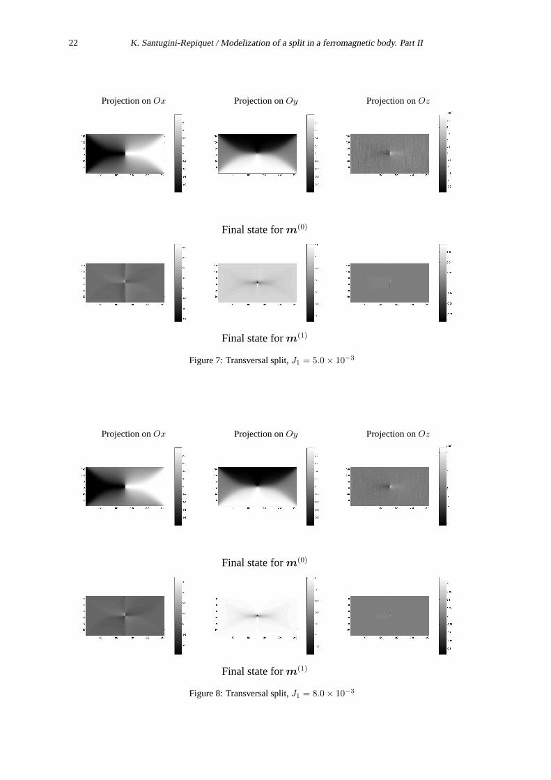
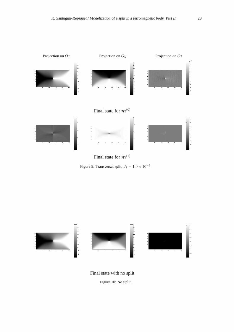
We analyze the equilibrium states obtained by our simulation. They represent the equilibriumstates and are presented in figures 3, 4, 5, 6, 7, 8, 9, and 10. When we raise the value ofJ1,the term of order0 of the equilibrium point magnetization becomes nearer to the equilibriumpoint of the magnetization with no split. It confirms that a strong super-exchange interactionfavors the alignment of the magnetization across the split.When the super-exchange is weak,the reversal of the magnetization across the split is brutal, which was expected. The quanti-ties of order1 show two unfinished vortices stretched across the transversal split, those twovortices lower in intensity as the super-exchange become stronger.
20 K. Santugini-Repiquet / Modelization of a split in a ferromagnetic body. Part II
Projection onOx Projection onOy Projection onOz
Final state form(0)
Final state form(1)
Figure 3: Transversal split,J1 = 0
Projection onOx Projection onOy Projection onOz
Final state form(0)
Final state form(1)
Figure 4: Transversal split,J1 = 1.0× 10⁻⁴
Conclusion
We have established here non trivial equivalent boundary conditions for a simpler geometrywhen surface interactions such as surface anisotropy and super-exchange are present, gener-alizing the results in part I [8]. We can now compute the effect of a split in a ferromagneticmaterial with a more accurate physical model involving interactions arising near the split.
K. Santugini-Repiquet / Modelization of a split in a ferromagnetic body. Part II 21
Projection onOx Projection onOy Projection onOz
Final state form(0)
Final state form(1)
Figure 5: Transversal split,J1 = 1.0× 10⁻³
Projection onOx Projection onOy Projection onOz
Final state form(0)
Final state form(1)
Figure 6: Transversal split,J1 = 2.0× 10⁻³
Future research will be concerned with non-void weak magnetic material filling the split.
22 K. Santugini-Repiquet / Modelization of a split in a ferromagnetic body. Part II
Projection onOx Projection onOy Projection onOz
Final state form(0)
Final state form(1)
Figure 7: Transversal split,J1 = 5.0× 10⁻³
Projection onOx Projection onOy Projection onOz
Final state form(0)
Final state form(1)
Figure 8: Transversal split,J1 = 8.0× 10⁻³
K. Santugini-Repiquet / Modelization of a split in a ferromagnetic body. Part II 23
Projection onOx Projection onOy Projection onOz
Final state form(0)
Final state form(1)
Figure 9: Transversal split,J1 = 1.0× 10⁻²
Final state with no split
Figure 10: No Split
24 K. Santugini-Repiquet / Modelization of a split in a ferromagnetic body. Part II
APPENDIX
A The Hr,s,t spaces
J.L. Lions et E. Magenes have in [5] introduce theHr,s spaces defined at (0.1) and provedtraces theorems. We refer the lector to this book for the details. We adapt this work to studythe Sobolev spaces on twice cylindrical domains, once in space and once in time.
A.1 Definition and traces theorems
LetO = B × (0,+L) andQT = O × (0, T ). Forr, s, t > 0, we define the spaces
Hr,s,t(QT ) = Ht(0, T ; L2(O)) ∩ L2(0, T ; Hs(0, L; L2(B))) ∩ L2(0, T ; L2(0, L; Hr(B))).
As in [5], we also define the spaces
Hr,s,t00, , (QT ) = Ht(0, T ; L2(O)) ∩ L2(0, T ; Hs(0, L; L2(B))) ∩ L2(0, T ; L2(0, L; Hr
00(B))),
Hr,s,t,00, (QT ) = Ht(0, T ; L2(O)) ∩ L2(0, T ; Hs
00(0, L; L2(B))) ∩ L2(0, T ; L2(0, L; Hr(B))),
Hr,s,t, ,00(QT ) = Ht
00(0, T ; L2(O)) ∩ L2(0, T ; Hs(0, L; L2(B))) ∩ L2(0, T ; L2(0, L; Hr(B))),
and,
Hr,s,t00,00, (QT ) = Hr,s,t
00, , ∩ Hr,s,t,00, , Hr,s,t
00, ,00(QT ) = Hr,s,t00, , ∩ Hr,s,t
, ,00,
Hr,s,t,00,00(QT ) = Hr,s,t
,00, ∩ Hr,s,t, ,00.
Lemma A.1 (Interpolation of theHr,s,t spaces).
[Hr1,s1,t1 ,Hr2,s2,t2 ]θ = H(1−θ)r1+θr2,(1−θ)s1+θs2,(1−θ)t1+θt2 , (A.1)
[Hr1,s100, ,H
r2,s200, ]θ = H
(1−θ)r1+θr2,(1−θ)s1+θs200, , (A.2)
[Hr1,s100,00,H
r2,s200,00]θ = H
(1−θ)r1+θr2,(1−θ)s1+θs200,00 . (A.3)
Theorem A.2 (Existence of traces). If v belongs toHr,s,t(QT ) then
1. If r > 12, and for all0 ≤ j,
∂jv
∂νj∈ Hµj ,νj ,λj(∂B × (0, L)× (0, T )),
with µjr=
νjs=
λjt=
r−j− 12
r.
2. If s > 12, then for all0 ≤ k < s− 1
2,
∂kv
∂zk∈ Hpk,qk(B × (0, T )),
with pkr= qk
t=
s−k− 12
s.
3. If s > 12, then for all0 ≤ l < t− 1
2,
∂lv
∂tl∈ Hαl,βl(B × (0, L)),
with αl
r= βl
s=
t−l− 12
t.
K. Santugini-Repiquet / Modelization of a split in a ferromagnetic body. Part II 25
Furthermore, the trace maps are linear continuous.
PROOF: We adapt the proof of Lions-Magenes [5]. The theorem is a direct consequenceof theorem 4.2 in Lions-Magenes [6]. To apply this theorem, we need interpolation resultsprovided in proposition 2.1 in [5] and Lemma A.1.
A.2 Conditions of compatibility
Proposition A.3 (First compatibility conditions). Let
fl =∂lv
∂tl∈ Hαl,βl(B × (0, L)),
gk =∂kv
∂zk∈ Hpk,qk(B × (0, T )),
hj =∂jv
∂νj∈ Hµj ,νj ,λj(∂B × (0, L)× (0, T )).
Then
1. If 1− 12(1r+ 1
s) > 0, then for allj, k ≥ 0 such thatj
r+ k
s< 1− 1
2
(1r+ 1
s
),
∂jgk∂νj
=∂khj∂zk
2. If 1− 12(1r+ 1
t) > 0, then for allj, l ≥ 0 such thatj
r+ l
t< 1− 1
2
(1r+ 1
t
),
∂jfl∂νj
=∂lhj∂tl
.
3. If 1− 12(1s+ 1
t) > 0, then for allk, l ≥ 0 verifying k
s+ l
t< 1− 1
2
(1s+ 1
t
),
∂jgk∂tl
=∂kfl∂zk
.
PROOF: D(QT ) is dense inHr,s,t(QT ) and the trace maps are continuous.
Proposition A.4 (Second compatibility conditions). With the same notations as the one usedfor the first conditions. We suppose thatB is the semi-spaceB = Rn−1 × R+ and thatL, T = +∞.Then
1. For all j, k such thatjr+ k
s= 1− 1
2
(1r+ 1
s
),
∫ +∞
σ=0
∫
Rn−1
∫ +∞
0
∣∣∣∣∂khj∂zk
(x′, σr, t)−∂jgk∂νj
(x′, σs, t)
∣∣∣∣2
dtdx′dσ
σ< +∞.
2. For all j, l such thatjr+ l
t= 1− 1
2
(1r+ 1
t
),
∫ +∞
0
∫
Rn−1
∫ +∞
0
∣∣∣∣∂lhj∂tl
(x′, z, σr)−∂jfl∂νj
(x′, σt, z)
∣∣∣∣2
dzdx′dσ
σ< +∞.
26 K. Santugini-Repiquet / Modelization of a split in a ferromagnetic body. Part II
3. For all k, l such thatks+ l
t= 1− 1
2
(1s+ 1
t
),
∫ +∞
0
∫
Rn−1
∫ +∞
0
∣∣∣∣∂kfl∂zk
(x′, xn, σt)−
∂lgk∂tl
(x′, xn, σs, x′)
∣∣∣∣2
dxndx′dσ
σ< +∞.
PROOF: It is a direct consequence of theorem 2.2 of Lions-Magenes [5]. We do it for
one inequality. We differentiateu and obtain that∂k
∂zk
(∂lu∂tl
)belongs toHµ,ν,λ(B×R+
z ×R+t ),
with µ
r= ν
s= λ
t= 1−
(ks+ l
t
). Since,1
ν+ 1
λ= 2, we can conclude.
Definition A.5. We define
F =∏
j<r− 12
Hµj ,νj ,λj(∂B×(0, L)×(0, T ))×∏
k<s− 12
Hpk,qk(∂B×(0, T ))×∏
l<t− 12
Hαl,βl(∂B×(0, L)).
Let F0 be the subspace ofF comprising functions(hj, gk, fl) satisfying both compatibilityconditions stated in Propositions A.3 and A.4.
LetΣ = ∂B × (0, L)× (0, T ). We state the principal extension theorem.
Theorem A.6 (Surjectivity of the trace map). The trace map
γ : Hr,s,t(QT ) → F0
v 7→ (hj, gk, fl)
is onto and has a continuous right inverse.
PROOF: We need interpolations equalities (A.2) and (A.3). We onlyneed to prove thesurjectivity. Let(fl, gk, hj) be inF0. Then, there existsϕ in Hr,s,t(QT ) such that∂
jϕ
∂νj = hjfor all 0 ≤ j < r − 1
2. And (fl − ∂ltϕ, gk − ∂kzϕ, 0) belongs toF0. Thus,gk − ∂kzϕ belongs
to Hpk,qk00, (R+
t × B). Using theorem 4.2 of Lions-Magenes [6], there existsψ in Hr,s,t(QT )
such that∂jψ
∂νj = 0 for all 0 ≤ j < r − 12, and ∂kψ
∂zk= gk − ∂kzϕ for all 0 ≤ k < s − 1
2.
And (fl − ∂ltϕ− ∂tψ, 0, 0) belongs toF0. Thus,fl − ∂ltϕ− ∂ltψ belongs toHαl,βl00,00(R
+z ×B).
By Theorem 4.2 of Lions-Magenes [6], there existsΦ in Hr,s,t(QT ) such that∂jψ
∂νj = 0 for all
0 ≤ j < r− 12, ∂
kψ
∂zk= 0 for all 0 ≤ k < s− 1
2, and∂
lψ
∂tk= hl−∂
ltϕ−∂
ltψ for all 0 ≤ l < t− 1
2.
u = ϕ+ψ+Φ belongs toHr,s,t(QT ) and has traces(fj, gk, hl). The construction also providethe continuous right inverse.
We know for the spacesHr,s and these spacesHr,s,t the compatibility relations. However,these relations ensure the surjectivity when all traces arepresents. Sometimes, we only wishto extend a subset of all traces. If the direct compatibilityrelations are verified, can wealways complete the mandatory traces by dummy traces such that all compatibility relationsare satisfied? We prove in two particular cases that no new indirect compatibility relationsare necessary. From now, we denote byx a vector ofRn with decompositionx = (x′, xn)wherex′ belongs toRn−1 andxn is scalar.z is the additional variable of space.t is the timevariable.
Theorem A.7. Let B be a bounded open set with a smooth boundary, andL and T twopositive real. Then, the maps
H2,2(B × (0, L)) → H12 (B × 0)× H
12 (B × L)× H
12 (∂B × (0, L)),
u 7→
(∂u
∂ν(x ∈ ∂B),
∂u
∂z(·, ·, 0),−
∂u
∂z(·, ·, L)
).
(A.4)
K. Santugini-Repiquet / Modelization of a split in a ferromagnetic body. Part II 27
and
H2,2,1(B × (0, L)× (0, T )) → H12, 12, 34 (∂B × (0, L)× (0, T ))× H
12, 34 (B × 0 × (0, T ))
× H12, 34 (B × L × (0, T )),
u 7→
(∂u
∂ν(x ∈ ∂B),
∂u
∂z(·, ·, 0, ·),
∂u
∂z(·, ·, L, ·)
).
(A.5)
are onto and have a continuous right inverse.
PROOF: By abstract consideration on Hilbert spaces, we only need toprove the surjec-tivity. By local map and partition of the unity, we reduce bothproblems to the caseL = +∞,T = +∞, andB = Rn−1×R+
xn. Letf1, g1 be inH
12 (Rn−1
x′ ×R+
z )H12 (Rn−1
x′ ×R+
xn). To apply
the surjectivity theorems of Lions-Magenes for map (A.4), we must constructf0, g0 such that(g1, f1, g0, f0) satisfy all compatibility relations. We first notice that there is no direct com-patibility condition betweenf1 andg1. Then, we constructg0 andf0 with Theorem A.8. Weuse the same method to prove the surjectivity of map (A.5). Toapply Theorem A.6, we useTheorem A.9 to constructg0 and, h0 satisfying the compatibility condition. Constructingf0is easy and anyway not necessary because of the way we proved Theorem A.6.
A.3 Completion of traces for the spaceH2,2(Rn−1 × R+)
Theorem A.8. There exists a linear continuous mapY from L2(0,+∞; L2(Rn−1)) to thespaceH1,1(Rn−1 × (0,+∞)) and fromH
12, 12 (Rn−1 × (0,+∞)) to the spaceH
32, 32 (Rn−1 ×
(0,+∞)). Moreover, there exists a constantC such thatY(f)(·, 0) = 0, and
∫ +∞
0
‖∂(Yf)∂z
− f‖2L2(Rn−1)
zdz ≤ C‖f‖
L2(0,+∞;H12 (Rn−1))
.
PROOF: Hereu is the partial Fourier transform ofu in the first two variables. We de-
fineY(f)(ξ, z) = χ(z√
1 + |ξ|2)∫ z0f(ξ, z)dz, whereχ is a smooth real function satisfying,
0 ≤ χ ≤ 1, with Supp(χ) ⊂ [0, 2] andχ = 1 in [0, 1]. Y is the application we were lookingfor. Verifying it is tedious but straightforward.
Theorem A.9. There exists a linear continuous mapA from H12, 12, 14 (Rn−1
x× R+
z × Rt) toH
32, 32, 34 (Rn−1
x× R+
z × Rt) and a constantC > 0 such thatA(f)(·, 0, ·) = 0, and
∫
z=0
∫
t
∫
x
∣∣∣∣∂A(f)
∂z− f
∣∣∣∣2
dxdtdz
z≤ C‖f‖2
L2(R+z ×Rt;H
12 (Rn−1
x )), .
PROOF: We first define theB operator with help from Theorem A.8. For allf inH
12, 12, 14 (Rn−1
x×R+
z ×Rt), we defineB(f)(t) asY(f(t)) for all time t. We then defineA(f)
asAf = χ(z(1 + |τ |2)14 )B(f), where the Fourier transform is only in time and whereχ is
smooth and satisfies.χ = 1 in (−L/4, 5L/4), andχ = 0 in ∁ (−L/2, 3L/2). A has therequired properties. The verification is straightforward but tedious.
28 K. Santugini-Repiquet / Modelization of a split in a ferromagnetic body. Part II
References
[1] R.A. Adams.Sobolev Spaces. Number 65 in Pure and Applied Mathematics. AcademicPress, New York-London, 1975.
[2] W.F. Brown. Micromagnetics. Interscience Publishers, 1963.
[3] S. Labbé and P. Leca. Résolution rapide des équations de Maxwell quasistationnaires :matrices Toeplitz multidimensionnelles. Application au micromagnétisme.C. R. Acad.Sci. Paris, Série I(t. 327):415–420, 1998.
[4] M. Labrune and J. Miltat. Wall structure in ferro / antiferromagnetic exchange-coupledbilayers : a numerical micromagnetic approach.Journal of Magnetism and MagneticMaterials, 151:231–245, 1995.
[5] J.L. Lions and E. Magenes.Problèmes aux limites non homogènes, volume 2 ofTravauxet recherches mathématiques. Dunod, 1968.
[6] J.L. Lions and E. Magenes.Problèmes aux limites non homogènes, volume 1 ofTravauxet recherches mathématiques. Dunod, Paris, 1968.
[7] V.G. Maz’ya. Sobolev Spaces. Springer Verlag, 1986.
[8] K. Santugini-Repiquet. Modelization of a split in a ferromagnetic body by an equivalentboundary condition: Part 1. the classical case: no surface energies present.AsymptoticAnalysis, 47(3–4):227–259, 2006.
[9] K. Santugini-Repiquet. Solutions to the Landau-Lifshitz system with nonhomogenousNeumann boundary conditions arising from surface anisotropy and super-exchange in-teractions in a ferromagnetic media.Nonlinear Anal., 65(1):129–158, July 2006.

![of use of the elements plates, shells, [] This · planes (modelization plates) or curve (modelization shells). The modelizations of grids intervene for the numerical modelization](https://img.pdfslide.net/doc/110x75/5c12dc2e09d3f2557b8c083e/of-use-of-the-elements-plates-shells-planes-modelization-plates-or-curve.jpg)