Modelling and Forecasting International Tourist Arrivals ...ira.lib.polyu.edu.hk/bitstream/10397/1126/2/09-Tourist Arrivals_En.pdf · 20 Haiyan Song Baogang Fei Modelling and Forecasting

20 Haiyan Song Baogang Fei

Modelling and Forecasting International TouristArrivals to Mainland ChinaHaiyan Song*, Baogang FeiThe Hong Kong Polytechnic University

Abstract:

The general-to-specific modelling approach is used to forecast tourist flows to mainland

China from eight major origin countries/regions over the period 2006-2015. The existing literature

shows that the general-to-specific methodology is a useful tool in modelling and forecasting tourism

demand at the destination level. With the aid of econometric models, the factors which contribute

to the demand for mainland China tourism have been identified. Empirical results reveal that the

most important factor that determines the demand for mainland China tourism is the economic

condition in the origin countries/regions. The “word of mouth” effect, the costs of tourism in

mainland China and the price of tourism in the competing destinations also have noticeable

influence on the demand for mainland China tourism. The generated forecasts suggest that mainland

China will face increasing tourism demand by residents from all the origin countries/regions

concerned while the growth rate of tourist arrivals from Korea is the most significant one. The

demand elasticities and the forecasts of tourist arrivals obtained from the demand models form the

basis of policy formulation for the tourism industry in mainland China.

Key words: Tourism demand, elasticity, econometric modelling, forecasting

1. Introduction

Due to its vast territory and extensive mystery, its civilization of over 5,000 years and numerous

places of attraction, mainland China has experienced a spectacular growth in inbound tourism

since the start of its open-door policy in 1978 and has fast become one of the world's top players

in tourism. During the last 20-odd years, tourism industry in mainland China has been one of the

fastest-growing industries in the national economy and one of the most significant foreign currency

earners (China Knowledge Press, 2004).

* Corresponding authorHaiyan Song, Chair Professor of Tourism, School of Hotel and Tourism Management, The Hong KongPolytechnic University, Email: [email protected] Fei, Research Associate, School of Hotel and Tourism Management, The Hong Kong PolytechnicUniversity; PhD Candidate, Dongbei University of Finance and Economics, Email: [email protected].

21Modelling and Forecasting International Tourist Arrivals to Mainland China

In 1978, mainland China only received about 1.81 million international tourists and merely

made an income of US$2.63 billion. In 2005, international tourism arrivals in mainland China

increased to 102.29 million, which was 56 times more than that in 1978, and mainland China was

the fourth most popular tourist destination in the world (World Tourism Organization [UNWTO],

2006). The World Tourism Organization has projected that mainland China will be the top tourism

destination in the world by 2020 (UNWTO, 2003). International tourism receipt in 2005 reached

US$29.29 billion, which was 11 times more than that in 1978, ranked number six in the world

(UNWTO, 2006). The majority of international visitors (about 83.16%) are compatriots from

Hong Kong, Macao and Taiwan. Foreign visitors exceeded 20 million for the first time in history

in 2005 and showed an impressive increase of 19.62% from 2004 (CNTA, 2006). Japan has been

the biggest source market for mainland China’s inbound tourism during the period 1978-2005,

accounting for about 20% of the total market followed by South Korea, USA, Australia, Canada,

and several western countries that have shown increasing interest in travelling to mainland China

recently.

Mainland China’s tourism industry faced big challenges during the financial crisis in 1997

and the SARS epidemic in 2003. For example, the total number of tourist arrivals dropped by

6.4% (6.25 million) due to SARS resulting in a substantial decline of tourist receipt of 14.7%

(US$2.99 billion). This shows that the industry is vulnerable to external shocks. Tourism

practitioners including policymakers and recreation facilities providers need to know how the

industry is impacted by the influencing factors. In addition, for planning and investment purposes,

accurate forecasts of the future trend of the international tourism demand in mainland China are

important. Now that the country is currently expecting a growth in inbound demand on account

of its deepening reform and success in hosting the Olympics in Beijing in the year 2008, the need

for accurate inbound tourism forecasts is even more imperative.

However, against this background, the studies on the demand for mainland China tourism

have been limited, especially by quantitative analysis (Kulendran & Shan, 2002). Even fewer attempts

have been made to forecast China’s inbound tourism (Turner & Witt, 2000). This is particularly

true when econometric methods are considered. In this connection, one main contribution of this

paper is that it employs the general-to-specific methodology to analyze the demand for mainland

China tourism. In achieving this, we have identified the key factors that contribute to the demand

for mainland China tourism and established the dynamic econometric models to account for the

effect of these factors on tourists’ choice of mainland China as a destination. Another main

contribution of this paper is the generation of the forecasts of tourist arrivals to mainland China

for the period of 2006-2015 with the aid of the estimated econometric models.

The rest of this paper is organized as follows. Section 2 reviews recent publications in the area

of tourism modelling and forecasting, which provides the rationale for using the chosen research

methodology for this study. Section 3 presents the models employed in this research for the analysis

of demand for mainland China tourism and explains the data used for the estimation of these

models. Section 4 contains empirical estimates of the inbound demand models. The forecasts of


tourist arrivals in mainland China for the period 2006-2015 are generated based on the estimated

models in Section 5 and Section 6 concludes the study.

2. Literature Review

It has been widely acknowledged that reliable tourism demand forecasts are important for

government and business for tourism planning, investment decision and policy formulation (Artus,

1972; Frechtling, 1996; Loeb, 1982; Song & Witt, 2006; Wong & Song, 2002). For example,

public and private tourism sectors require meaningful estimates of tourism demand in order to

ensure efficient allocation of scarce resources, and demand elasticities provide useful information

on the comparative advantages of tourism in product diversification (Quayson & Var, 1982).

Since the beginning of the 1960s, extensive studies have been carried out on tourism demand

forecasts through either qualitative approaches or quantitative approaches. The focus of this study

is, however, on quantitative forecasting methods.

Generally speaking, the existing literature on tourism demand analysis using quantitative

approaches falls into two major groups: i) non-causal (mainly time-series) methods, which extrapolate

historic trends of tourism demand into the future without considering the underlining causes of the

trends, and ii) casual (econometric) methods, which use regression analysis to estimate the quantitative

relationship between tourism demand and its determinants. Whilst the non-causal time-series

approaches are useful tools for tourism demand forecasting, a major limitation of these methods is

that they cannot be used for policy evaluation purpose. As pointed out by Song, Wong, and Chon

(2003), econometric models (which are mainly causal models) are superior to the time-series approaches

for the reason that econometric models are carefully constructed based on economic theory and

therefore can be used for policy evaluation. As a result, a large body of literature has been published

on tourism demand forecasting using econometric techniques (e.g. Crouch, Schultz, & Valerio,

1992; Hiemstra & Wong, 2002; Kulendran & King, 1997; Morley, 1994; Smeral & Weber, 2000;

Smeral, Witt, & Witt, 1992; Song & Witt, 2000; Song, Witt, & Jensen, 2003; Tan, McCahon, &

Miller, 2002; Witt & Witt, 1992). Li, Song, and Witt (2005) provided a comprehensive review of

these studies. In this paper, considerable attention is devoted to the econometric methodology.

Tourism demand normally refers to the demand for tourism-oriented products such as

accommodation, food service, transportation, etc., and is usually measured by tourist arrivals,

tourist expenditures, average length of stay, bed occupancy or activities engaged in the visit, etc.

Tourist arrivals are the most frequently used measure for tourism demand modelling and usually

analyzed by country of residence (nationality) or by purpose of visit. Lim (1997a) studied 100

empirical tourism research works up to 1994 and found 51of them used tourist arrivals as dependent

variable followed by tourist expenditure (49) in real or nominal terms. In a more recent literature

survey, Li et al. (2005) pointed out that amongst the 84 selected studies published since 1990, 53

of them used tourist arrivals as the dependent variable and only 16 employed tourist expenditure

as the dependent variable.


Although tourism demand could be affected by a wide range of factors such as economic,

attitudinal and political factors, the majority of studies focus on economic factors to obtain a

satisfactory explanation. In this context, income in the origin country/region is regarded as one of

the most influential factors that has a positive effect on tourism demand. In cases where income is

not included in a model, there is usually some form of aggregated expenditure variable in its place

(Witt & Witt, 1995). Crouch (1994) revealed that the income is the most important explanatory

variable, and income elasticity generally exceeds unity but below 2.0, which implies that international

travel is a luxury good. A considerable diversity of income variables had been used in tourism

demand analysis over the past four decades. Edwards (1988, 1991) argued that increases in real

disposable income, defined as the income after tax and after necessities (food, clothing, housing,

etc.) have been paid for among those population prone to take long haul holidays aboard, cause

the demand for tourism to increase. Lim and McAleer (2002) compared the explanatory power of

real Gross Domestic Product (GDP) and real private consumption expenditure in modelling tourist

arrivals to Australia from Malaysia. Moreover, Gross National Product (GNP) and Gross National

Income (GNI) were also used as alternative income variables in a number of studies on business

travel or combination of business travel and leisure travel. As pointed out by Song, Romilly, and

Liu (2000), Kulendran and Witt (2001), and Turner and Witt (2005), real personal disposable

income (PDI) were the most appropriate proxy to be included in the demand models concerning

holidays or visiting friends and relatives (VFR). If attention focuses on business visit, then a more

general income variable (such as national income) should be used. Additionally, Gonzalez and

Moral (1995) and Song, Witt, et al. (2003) made innovative attempts in tourism modelling to use

private consumption expenditure and industrial production index, respectively.

Economic theory indicates that prices also play an important role in determining tourism

demand, as tourism demand can be interpreted as the demand for specific tourism goods and

facilities. It is clear that the prices should include the prices of goods and facilities relating to both

tourism destination and substitution destinations. However, the price variables are normally difficult

to determine because of the enormous diversity of the products purchased by tourists. Edwards

(1988) summarized the methods used to establish these proxies of prices variables. Tourism demand

analysis in the 1960s and 1970s usually defined the price variable as a ratio of price indexes in the

destination to a weighted price index in the origin country and substitute destinations. In recent

demand studies, the impact of prices on the tourism demand is usually considered by two separate

price variables: the own price of tourism and the substitute prices in alternative destinations.

The own price of tourism is defined as the relative cost of travelling abroad to domestic travel

and it includes two components: the cost of living for tourist at the destination and the travel cost

to the destination. Due to potential multi-colinearity problems and difficulties in obtaining reliable

data, the cost of the travelling to the destination have been omitted in most of the studies with

some exceptions, such as Ledesma-Rodríguez, Navarro-Ibáñez, and Pérez-Rodríguez (2001), who

included such cost in their models by employing oil or gasoline costs as a proxy of travel costs. The

cost of living in destination consists of two components. One is the relative price of tourism in the


destination to that of the origin country/region, which evaluates the real expenditure at destination.

The other is the relative exchange rate between the origin country/region and the destination.

Normally, tourists are more aware of exchange rate than the living cost in destination. As Song and

Witt (2006) stated, an exchange rate in favour of the origin country’s currency would result in

more tourists visiting the destination from the origin country. The specific results of the empirical

study (Witt & Martin, 1987b) indicated that the consumer price index (CPI, either alone or

together with the exchange rate) is a reasonable proxy for the cost of living while exchange rate on

its own, however, is not an acceptable one. The own price could be calculated as an exchange rate

adjusted price index by dividing the relative CPI index between the destination and origin countries/

regions by relative exchange rate between those two countries. The justification for this method is

that the level of price in the destination may work against beneficial exchange rates.

The influence of substitute prices on tourism demand is less apparent than own price of tourism.

According to the review article by Lim (1997a), less than 10 of the 100 studies published before 1990

included substitute prices in the demand models. However, over the past 15 years, 37 of 84 studies

incorporated the substitute price as an independent variable (Li et al., 2005) in tourism demand

research. Martin and Witt (1988) calculated the substitute price based on a weighted average index

where the weights were determined by the market shares of the competing destinations, and the

weights were allowed to change over the estimation period to cater for changing trends. Their empirical

results support the hypothesis that substitute prices play an important role in determining the demand

for international tourism, but there is considerable variation in importance according to the origin-

destination pairs and travel mode. So far, there are two forms of substitute prices that have been

adopted. One allows for the substitution between the destination and a number of competing

destinations separately (Kim & Song, 1998). The other one calculates the cost of tourism in the

destination under consideration relative to the costs of living in the competing destinations, and this

relative price is also adjusted by relevant exchange rates. The cost of living of the competing destinations

is calculated as a weighted index with the weight being the market share (arrivals or expenditures) of

each competing destination under consideration (Song & Witt, 2000). This substitute price variable

has been frequently used in recent empirical studies.

In addition to the variables mentioned above, marketing expenditure, consumer taste,

consumer expectations and habit persistence, population and one-off events, are also potentially

important factors that could be incorporated in tourism demand models (Song & Witt, 2000).

Marketing expenditure can play an important role in inbound tourism demand, as promotions are

normally conducted to increase the attractiveness of the tourism destination where tourism is a

major industry in the economy. Crouch et al. (1992) estimated the impact of international marketing

activities of Australian Tourist Commission on tourist arrivals and the results show that the marketing

variable is significant in the empirical models of their study. Only a small number of studies, with

the exceptions of Crouch et al., Dritsakis and Athanasiadis (2000), Law (2000), have included the

marketing expenditure variable in their empirical analyses because of the unavailability of the

marketing expenditure data.


Witt and Martin (1987a) discussed that the time trend represents tourists’ taste change as

well as population increases. The lagged dependent variable describes tourists’ expectations, habit

persistence, “word of mouth” effect and tourism product supply constraints. The problem of

including the time trend and lagged dependent variables in tourism demand analysis is that we

cannot locate exactly which factor the model really captures. Lagged explanatory variables are also

included in the demand model to capture the dynamic effect (Lim, 1997).

Zhang, Wei, and Liu (2004) studied the demand for tourism in mainland China by taking

account of the influence of the political system, macroeconomic policies, the forthcoming Olympic

Games and other influential factors using the qualitative approach. However, very little attention

has been paid to the quantitative analysis of demand for mainland China tourism over the past

decades. Wang and Zeng (2001) and Wu, Ge, and Yang (2002) introduced the possibility of using

artificial neural network (ANN) in inbound tourism analysis without any support of empirical

evidence. Yin, Hu, and Qiu (2004) applied the support vector machine (SVM) model in Yunnan

tourism demand data. The only noteworthy studies on mainland China tourism demand are

Kulendran and Shan (2002) and Turner and Witt (2000). The former examined mainland China’s

monthly inbound travel demand using the conventional seasonal autoregressive moving average

(ARMA) model. The latter used a technique known as structural integrated time-series econometric

analysis (SITEA) by combining both time-series and econometric methodologies to forecast inbound

tourism to mainland China. The SITEA approach is a specific-to-general modelling approach,

which starts with a relatively simple model. The simple model is then expanded to include causal

variables if the simple model does not perform well. As a result, the final model used for forecasting

could be very complex.

An alternative modelling approach is known as general-to-specific approach1. This

methodology was originally proposed by Davidson, Hendry, Saba, and Yeo (1978) and subsequently

modified by Hendry and von Ungern-Sternberg (1981) and Mizon and Richard (1986). Full

development of the general-to-specific modelling approach has only taken place recently, coupled

with the development of co-integration and error correction methodologies (ECM) (Hendry,

1995). The general dynamic autoregressive distributed lag model (ADLM) encompasses a number

of specific models (simple autoregressive, static, growth rate, leading indicator, partial adjustment,

finite distributed lag, dead start, and error correction) and the general model can be reduced to

one of the specific models by imposing certain restrictions on the parameters in the model. On the

basis of various restriction tests and diagnostic statistics, the final models could be selected and

used for forecasting and policy evaluation purpose.

1 Detail is discussed in Song & Witt, “Tourism Demand Modelling and Forecasting”, 2000, pp. 28-51.


3. The Model

This section deals with the issues related to the model specification. In this study the general-

to-specific model is used to forecast the demand for mainland China tourism by tourists from eight

major origin countries/regions. The majority of international visitors in mainland China are

compatriots. Statistics published by CNTA show that tourists from Hong Kong and Taiwan

accounted for about 61.77% of the total tourist arrivals in mainland China in 2005. In terms of

the foreign visitors, statistics in the same year show that the followings are the major tourism origin

countries: Japan (16.74%), Korea (17.5%), UK (2.47%), USA (7.68%), Australia (2.38%) and

Canada (2.12%). One reason why this approach is selected is that it has a clear strategy in model

specification, estimation and selection, and therefore does not suffer from the extensive data-

mining problem that is associated with many other modelling methodologies. Another advantage

of this approach is that the general-to-specific method starts with a dynamic ADLM within which

the ECM is embedded, the dynamic characteristics of demand behaviour are allowed for, and the

spurious regression problem also can be overcome.

3.1 Determinants of tourism demand

As mentioned earlier, tourism demand in this study is measured by tourist arrivals from the

major origin countries/regions. The economic conditions that are relevant for the demand for

tourism include tourism prices in mainland China, the availability of and tourism prices for

substitute destinations, and incomes of tourists in their home countries/regions. In this paper the

following demand function is proposed to model the demand for mainland China tourism by

residents from a particular origin country/region i:

where TAit is the number of tourist arrivals in mainland China from origin country/region i at time

t ; Yit is the income level of origin country/region i at time t ; Pit, is the own price of tourism in

mainland China for tourists in the origin country/region i at time t ; Pist is the substitute price at

time t , and eit is the random error and is used to capture the influence of all other factors that are

not included in the demand model. The measurement issue and the sources of the variables

included in the demand Eq. (1) are explained below.

The dependent variable TAit is measured by the number of arrivals from a particular original

country/region i in mainland China and the data were obtained from the Tourism Statistical

Yearbook published by World Tourism Organization.

The income variable, Yit, is income in origin country/region i measured by the index of real

GDP, and was collected from International Financial Statistics Yearbook published by International

Monetary Fund (IMF) for all countries/regions. The personal disposable income may be the best

proxy to measure the income, but due to data unavailability and a large proportion of business

travellers in tourist arrival data this proxy is not used in this study.

TAit = AYit Pit Psit eit (1)b2 b3 b4


The definition of the own price variable in this study is

where CPIcn and CPIi are the consumer price indexes for mainland China and origin country/

region i, respectively; EXcn and EXi are the exchange rate indexes for mainland China and origin

country/region i respectively. The exchange rate is the annual average market rate of the local

currency against the US dollar.

The substitute price variable, Pist, is defined as a weighted index of selected countries/regions.

Both geographic and cultural characteristics are taken into account. Finally, Taiwan, Singapore,

Thailand, South Korea and Hong Kong were considered in this study to be substitute destinations

for mainland China.

where j = 1, 2, 3, 4 and 5 representing Taiwan, Singapore, Thailand, South Korea and Hong Kong,

respectively; wij is the share of international tourism arrivals for country/region j, which is calculated

from wij = TAij ∑ TAij , and TAij is the inbound tourist arrivals of substitute destination j from

origin country/region i.

3.2 Model specification

According to Song and Witt (2000), one major feature of the power function (Eq. (1)) is that

it can be transformed into a log linear specification, which can be estimated easily using ordinary

least squares (OLS). After taking logarithm of Eq. (1), we have

where b1 = 1nA, «it = 1neit , and b2, b3 and b4 are income, own price and cross price elasticities,

respectively. We expect that b3 < 0 (the price of tourism would have a negative influence on

tourism demand) while b2 and b4 > 0 (the income level of the origin country/region and substitute

price of tourism would have positive impacts on tourism demand). The above equation is a static

model and does not take into account the dynamic issue of tourists’ decision process. In order to

capture the dynamic feature of tourism demand, a model specification known as ADLM is used in

this study. With a lag length of 1, the simplest ADLM for Eq. (4) is given by Eq. (5).

Pit = (2)CPIcn EXcn

CPIi EXi

Pit = (3)CPIj

EXj

wij∑n

j=1

5

j=1

1nTAit = b1+b21nYit+b31nPit+b41nPist+«ist (4)


Extra attention should be placed on the coefficients in Eq. (5) which are definitely not

demand elasticities while the coefficients b2, b3 and b4 in Eq. (4) are. Some algebraic manipulations

are needed to get the demand elasticities, as indicated by Song and Witt (2000). The long run

demand function for Eq. (5) can be written as

where b2 = , b3 = and b4 = .

1nQit = + 1nPit + 1nYit+ 1nPit (6)a1

(1–a2)

(a3+a4)

(1–a2)

(a5+a6)

(1–a2)

(a7+a8)

(1–a2)s

(a3+a4)

(1–a2)

(a5+a6)

(1–a2)

(a7+a8)

(1–a2)

4. Estimates of the Demand Models

This section presents the empirical results from the estimation of the models discussed in

Section 3. All models are estimated using annual data from 1985 to 2005. In estimating Eq. (5), a

number of dummy variables were also included to capture the influence of one-off events on the

demand for mainland China tourism. These dummy variables include: the Asian financial crisis in

1997, D97, which takes a value of 1in 1997 and 0 otherwise; the 911 terrorism attack in 2001 in USA,

D911, which takes a value of 1 in 2001 and 0 otherwise; and the SARS in China in 2003, DSARS, which

takes a value of 1 in 2003 and 0 otherwise. Therefore, the initial ADLM now becomes

OLS is employed to estimate model parameters.

Before the model estimation, the data were tested for unit roots and co-integration. Augmented

Dickey Fuller (ADF) test and Johansen maximum likelihood procedure were used for this purpose.

All the variables are found to be integrated of order 1 and at least one co-integration relationships are

identified among the variables included the demand models. A model reduction procedure was

followed to eliminate the unimportant variables which are either insignificant statistically or inconsistent

with economic theory (i.e. their coefficients have wrong signs) in Eq. (7) for all the 8 origin countries/

regions. Table 1 presents the estimated final models for all origin countries/regions.

In general, all the models fit the data well with relative high adjusted R2s ranging from

between 0.936 to 0.995. Particularly, the results in Table 1 show that the lagged-dependent

variable is significant in the Australia, Japan, Hong Kong and USA models. This suggests that the

�word of mouth� effect and/or consumer persistence features importantly in the demand for

mainland China tourism by tourists from these four origin countries/regions. This might explain

1nTAit = a1+a21nTAit-1+a31nYit+a41nYit-1+a51nPit+a61nPit-1

+a71nPis+a81nPist-1+a9D97+a10D911+a11DSARS+eit (7)s s

1nTAit = a1+a21nYit-1+a31nYit+a41nYit-1+a51nPit+a61nPit-1

+a71nPist+a81nPist-1+«is (5)


why these four countries/regions are among the top five tourism generating countries/regions for

mainland China. The income variable is significant in all but Japan and Hong Kong models

suggesting that the income level of the origin country is an important determinant of international

tourism demand in mainland China. The price of tourism and substitute price are only significant

in 4 out of the 8 models suggesting that the price of tourism and cost of tourism in competing

destinations are less important in influencing the demand for mainland China tourism compared

with the income variable.

Table 1 Estimates of the demand models: the dependent variable is LnTAit

Variable AUS CA JP KOR HK TW UK USA

C -2.403* a -2.086** 0.901 -8.215* 0.294 6.162* 0.136 -0.153(-3.844) (-1.974) (1.069) (-14.970) (0.594) (13.600) (0.112) (-0.194)

LnTAit-1 0.717* 0.946* 0.988* 0.437*

(5.871) (15.739) (34.198) (2.506)

LnPit -0.629 -0.777(-2.555) (-3.036)

LnPit-1 -1.230* -0.930* -0.694*

(-4.739) (-5.473) (-2.309)

LnYt 7.735* 4.841* 2.714* 1.729*

(5.226) (39.546) (10.207) (3.103)

LnYt-1 1.324* -4.634* 1.916*

3.443 (-3.146) (17.967)

LnPSt -2.410* -0.592*

(-3.269) (-3.389)

LnPSit-1 2.860* 1.316* 0.392*

(4.257) (4.791) (2.404)

D97 -0.234*

(-2.208)

D911

DSARS -0.384* -0.191* -0.257* -0.460*

(-3.063) (-1.869) (-2.433) (-4.765)

R2 0.973 0.978 0.936 0.995 0.984 0.944 0.973 0.979

ACb -1.300 -1.365 -0.480 -1.702 -2.401 -0.623 -1.715 -1.832

SCc -1.101 -1.066 -0.330 -1.461 -2.301 -0.524 -1.466 -1.483

kçíÉW=~W=qÜÉ=ÑáÖìêÉë=áå=é~êÉåíÜÉëáë=~êÉ=íJëí~íáëíáÅëX=G=~åÇ=GG=êÉéêÉëÉåíë=RB=~åÇ=NMB=ëáÖåáÑáÅ~åí=äÉîÉäë

êÉëéÉÅíáîÉäóX=ÄW=^â~áâÉ=áåÑçJÅêáíÉêáçåX=ÅW=pÅÜï~êò=ÅêáíÉêáçåK


The Asian financial crisis in 1997 seems to have had a negative impact on the demand for

mainland China tourism. In particular, the financial crisis reduced tourism arrivals from South

Korea and Hong Kong. The 911 event in the USA does not have any impact on the demand for

mainland China tourism by residents from all 8 countries/regions. The SARS epidemic in 2003,

had a significantly negative impact on the demand for mainland China tourism, specifically the

SARS dummy is significant in the Australia, UK and USA models.

Based on the estimated demand models in Table 1, demand elasticities are derived and are

presented in Table 2. The results show that Canada, USA, UK and Japan tourists seem very

sensitive to the prices of tourism in mainland China, especially the own price elasticity in the

Japan model is as low as -11.75. The demand for mainland China tourism by the UK residents is

price inelastic while the tourists from Australia, Korea, Hong Kong and Taiwan seem do not pay

much attention to tourism prices when they make travel decisions to mainland China. Ranging

from 1.916 to 4.841, the income elasticities imply that a 1-percent increase (decrease) in real GDP

in Australia, Canada, Korea, Taiwan, UK and USA would result in more than 1 percent increase

in tourist arrivals in mainland China for these countries/region, given that other variables keep

unchanged. Therefore, mainland China needs to accurately predict the business conditions associated

with these 6 origin countries/regions in order to deal with the fluctuations in the demand for

mainland China tourism. In addition, cross price elasticities show that tourists from Canada,

Korea and UK are aware of the prices of tourism in the substitute destinations (substitute effect)

while tourists from the USA tend to visit mainland China and the competing destinations on the

same trip (complementary effect).

Table 2 Estimated demand elastictities

Country/Region Own Price Elasticity Income Elasticity Cross Elasticity

Australia � 4.675 �

Canada -1.230 3.101 0.45

Japan -11.751 � �

Korea � 4.841 1.316

Hong Kong � � �

Taiwan � 1.916 �

UK -0.930 2.714 0.392

USA -2.615 3.073 -1.052


TEST AUS CA JP KOR HK TW UK USA

CSQA 1.327 0.462 1.696 0.433 2.155 0.027 0.790 0.402

CSQN 0.942 0.198 2.076 0.606 6.421* 1.361 2.061 0.108

CSQH 3.740 8.501 7.678 4.198 0.389 6.155* 11.888 8.171

CSQF 2.208 0.002 0.462 3.347 0.000 0.391 0.022 0.713

CSQS 0.887 0.029 2.058 1.520 1.166 0.039 1.267 0.901

CSQAH 0.027 0.537 0.316 2.466 0.273 9.372* 0.608 0.434

kçíÉW=G=êÉéêÉëÉåíë=Ñ~áäáåÖ=íç=é~ëë=íÜÉ=Çá~ÖåçëíáÅ=íÉëí=~í=RB=ëáÖåáÑáÅ~åí=äÉîÉäK

In this study, the following diagnostic tests are carried out: the Breusch (1978) and Godfrey

(1978) Lagrange multiplier chi-square test for serial correlation (CSQA), the White (1980) Chi-

square test for heteroscedasticity (CSQH), the Jarque and Bera (1980) Chi-square test for

nonnormality (CSQN), the Chow (1960) test for model stability (CSQS), Engle (1982) ARCH

test (CSQAH) for autoregressive conditional heteroscedasticity and the RESET (Ramsey, 1969)

misspecification test (CSQF). If the final model passes all these tests, the models are data admissible,

encompassing and consistent with theory (Hendry & Richard, 1983). Table 3 presents the results

of all diagnostic tests. The diagnostic statistics show that most models pass all six tests with the

Hong Kong model only failed CSQN, and the Taiwan model failed CSQH and CSQAH. Overall,

given the small sample size (only 21 observations for all the variables) the estimated demand

models could be regarded as well specified and can be used for forecasting.

Table 3 Results of diagnostic tests


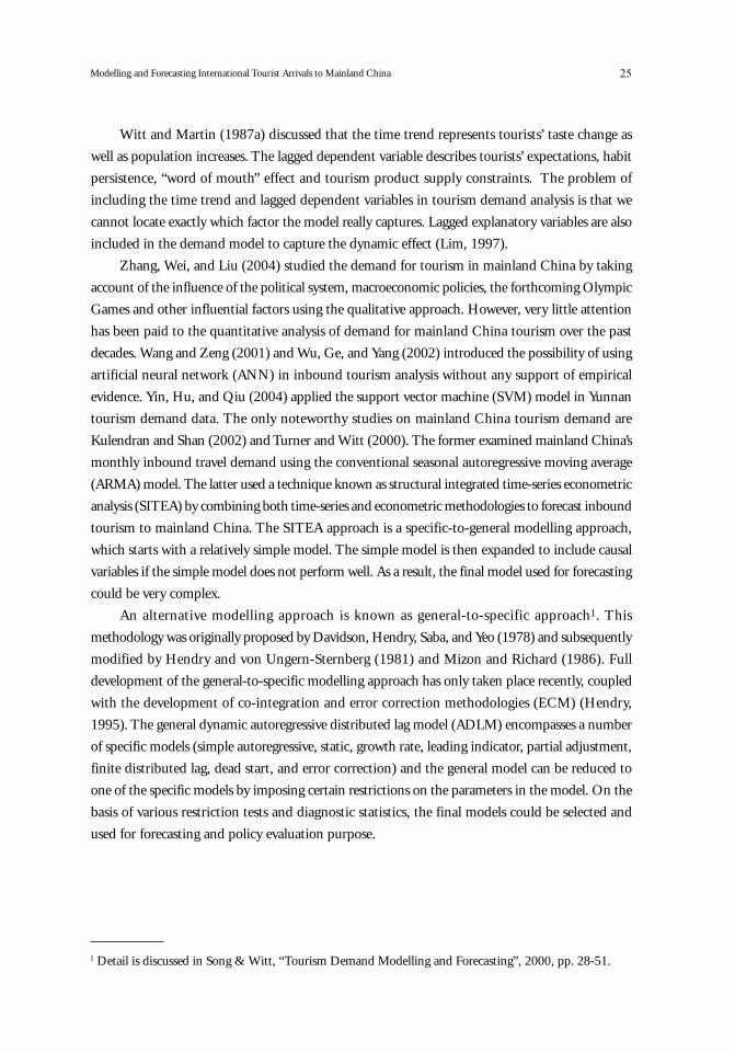
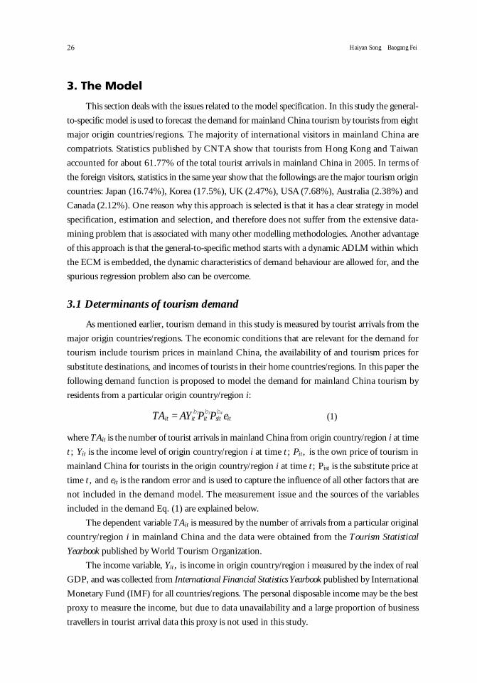
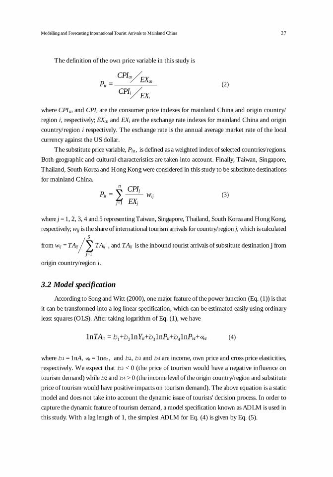
5. Forecasts

The estimated demand models presented in the previous section are used to forecast tourist

arrivals for the period 2006-2015.

Before we generate the forecasts of tourist arrivals for each of these origin countries/regions,

we need to predict the explanatory variables first. The method used for forecasting the explanatory

variables is exponentially smoothing. This method is easy to use and capable of producing reliable

forecasting for the explanatory variables in tourism demand models (Song & Witt, 2000). Since

all the explanatory variables are annual time series, which have either distinctive trends or stochastic

trends, the Holt-Winters non-seasonal models is used.

Once the forecasts of the explanatory variables are generated, they can be substituted into the

forecasting models given in Table 1 and the forecasts of the dependent variables are then calculated

based on the estimated coefficients of the models. The initial observation in the forecast sample

will use the actual lagged value of the dependent variable. The forecasts for the subsequent periods

will use the previously forecasted values of the lagged dependent variable. The projected tourist

arrivals for all the 8 origin countries/regions are presented in Table 4. Since the variables in the

demand models are all in logarithm, the forecast values of tourism arrivals are also in logarithm.

The actual tourist arrivals taking the anti-log operation of these values are shown in Figures 1-8.


Cou

ntry

/Reg

ion

2006

2007

2008

2009

2010

2011

2012

2013

2014

2015

Ann

ual G

row

th R

ate

Aus

tral

ia58

7411

6979

7582

2088

9621

8711

2108

313

0199

615

0859

617

4507

320

1621

023

2748

314

.9%

Can

ada

4856

0454

1082

6010

0366

7560

7414

8882

3603

9148

1210

1612

211

2865

112

5364

29.

9%

Japa

n34

8842

236

1124

137

5959

239

3505

041

3962

043

7576

446

4642

549

5507

353

0575

757

0317

25.

0%

Kor

ea50

2718

758

9417

574

0212

992

9587

611

6741

1514

6607

9818

4115

8923

1219

7529

0374

5836

4663

462.

1%

Hon

g K

ong

7615

7360

8254

8439

8939

1152

9671

0523

1045

3247

311

2883

831

1217

9233

013

1286

610

1413

9621

515

2151

589

7.2%

Tai

wan

4334

543

4672

144

5060

318

5480

743

5936

098

6429

285

6963

447

7541

989

8168

598

8847

267

7.4%

UK

4177

4044

9977

4946

4454

3744

5977

1865

7050

7222

7179

3967

8727

7995

9414

8.7%

USA

1928

030

2271

903

2644

967

3063

062

3539

056

4084

886

4712

814

5436

214

6270

123

7231

685

14.1

%

Tab

le 4

Fo

reca

sts

of

Tou

rism

Arr

ival

s in

Ch

ina


Figure 1

160000000

140000000

120000000

100000000

80000000

60000000

40000000

20000000

02006 2007 2008 2009 2010 2011 2012 2013 2014 2015

Forecasts of Tourist Arrivals from Hong Kong

Figure 2

40000000

35000000

30000000

25000000

20000000

15000000

10000000

5000000

02006 2007 2008 2009 2010 2011 2012 2013 2014 2015

Forecasts of Tourist Arrivals from Korea

Figure 3

10000000

9000000

8000000

7000000

6000000

5000000

4000000

3000000

2000000

1000000

02006 2007 2008 2009 2010 2011 2012 2013 2014 2015

Forecasts of Tourist Arrivals from Taiwan


Figure 4

8000000

7000000

6000000

5000000

4000000

3000000

2000000

1000000

02006 2007 2008 2009 2010 2011 2012 2013 2014 2015

Forecasts of Tourist Arrivals from USA

Figure 5

6000000

5000000

4000000

3000000

2000000

1000000

02006 2007 2009 2010 2011 2012 2013 2014 2015

Forecasts of Tourist Arrivals from Japan

2008

Figure 6

2500000

2000000

1500000

1000000

500000

02006 2007 2008 2009 2010 2011 2012 2013 2014 2015

Forecasts of Tourist Arrivals from Australia


1400000

1200000

1000000

800000

600000

400000

200000

02006 2007 2009 2010 2011 2012 2013 2014 2015

Forecasts of Tourist Arrivals from Canada

2008

Figure 8

1200000

1000000

800000

600000

400000

200000

02006 2007 2008 2009 2010 2011 2012 2013 2014 2015

Forecasts of Tourist Arrivals from UK

Figure 7

6. Conclusion

In this paper the demand for mainland China tourism measured by tourist arrivals is modelled

and forecast using the general-to-specific approach. Tourist arrivals from 8 major origin countries/

regions, namely Hong Kong, Taiwan, Japan, Korea, UK, USA, Australia and Canada, are considered.

The lagged dependent variable, own price, substitute price, income and several dummy variables

were included in the demand models. The sample used in model estimation covers the period

1985-2005. Following a rigorous statistical testing procedure, the models that pass the statistical

tests and are consistent with the demand theory were selected for the purpose of policy evaluation

and forecasting. The estimates of the demand models show that the demand for mainland China

tourism is heavily influenced by the economic conditions in the origin countries/regions except

Japan and Hong Kong. Therefore, it is important for policymakers in mainland China to closely

monitor the economic conditions in these source markets.


The “word of mouth” effect or the behavioural persistence of tourists features significantly in

the demand for mainland China tourism by tourists from Australia, Japan, Hong Kong and USA.

This might explain why these four countries/regions are among the top five tourism origin countries/

regions for mainland China. The policy implication of this is that the suppliers of tourism products/

services in mainland China should improve their service quality and upgrade their brand images in

order to attract more tourists.

The cost of tourism in mainland China is another noticeable factor that influences the demand

for mainland China tourism. The price elasticity ranged from -0.93 to -11.751 suggesting that

there is a significant variation between origin countries/regions in terms of the responsiveness of

tourism demand to changes in the costs of tourism in mainland China. The price change in

mainland China seems to have a larger impact on the demand for mainland China tourism by the

Japanese residents (with the outstanding price elasticity of -11.751).

The price of tourism in the competing destinations also has a role to play in determining the

demand for mainland China tourism. The effect is, however, comparatively weak as it only affects

tourist flows from Canada, South Korea, UK and USA. An increase in tourism price in the alternative

destinations will result in a bigger increase in the tourist flow from Korea to mainland China while

a similar increase (decrease) in tourism price in the alternative destinations will result in a smaller

increase (decrease) in the tourist flows from Canada and UK to mainland China. The cross price

elasticity in the USA model indicates that tourists from the USA tend to visit mainland China and

the competing destinations on the same trip (complementary effect), as the estimated cross price

elasticity is -1.052.

Ex post forecasts over the period 2006 to 2015 are generated from the estimated final models,

which provide some useful information for tourism practitioners including recreation facilities

providers and government. The forecasting results show that the growth of tourist arrivals from

Korea is expected to be the strongest among the eight origin countries/regions. Markets such as

Australia, USA and Canada also show significant increases over the forecasting period, but to a less

extent. The forecasts for Hong Kong, Japan, Taiwan and UK show that demand for mainland

China tourism by residents from these origin countries/regions are likely to increase over the

forecasting period, but the growth rates of these countries/regions are much smaller than that of

Korea, Australian, USA and Canada. Hong Kong is predicted to be the largest source market for

mainland China tourism over the forecasting period.

The forecasts in this study were generated based on the single equation approach and the

sample size of the variables is small. It is likely the estimated models may suffer from small sample

bias. A future extension of this study could be to use the panel data approach (data on 8 countries/

regions over 20 years) to estimate the demand model with a view to reduce the small sample bias.

Acknowledgement

The authors acknowledge the financial support of the Hong Kong Polytechnic University’s

Niche Area Research Fund.


ReferencesArtus, J. R. (1972). An empirical analysis of international travel. IMF Staff Papers, 19, 579-614.

Breusch, T. (1978). Testing for autocorrelation in dynamic linear models. Journal of Australian EconomicPapers, 17(31), 334-355.

China Knowledge Press (2004). China tourism industry: Market analysis and outlook. Singapore: Author.

China National Tourism Administration (CNTA) (2006). Retrieved October 3, 2006, from http://www.cnta.com

Chow, G. C. (1960). Test of equality between sets of coefficients in two linear regressions. Econometrica, 28(3), 591-605.

Crouch, G. I. (1992). Effect of income and price on international tourism. Annals of Tourism Research, 19(4),643-664.

Crouch, G. I. (1994). The study of international tourism demand: A review of findings. Journal of TravelResearch, 32(1), 12-23.

Crouch, G. I., Schultz, L., & Valerio, P. (1992). Marketing international tourism to Australia: A regressionanalysis. Tourism Management, 13(2), 196-208.

Davidson, J., Hendry, D. F., Saba, F., & Yeo, S. (1978). Econometric modelling of the aggregate time seriesrelationships between consumers expenditure and income in the United Kingdom. Economic Journal, 88,661-92.

Dritsakis, N., & Athanasiadis, S. (2000). An econometric model of tourist demand: The case of Greece.Journal of Hospitality and Leisure Marketing, 7(2), 39-49.

Edwards, A. (1988). International tourism forecasts to 1999 (EIU Special No. 1142). London: EconomistPublications.

Edwards, A. (1991). The European long haul travel market: Forecasts to 2000. London: Economist IntelligenceUnit.

Engle, R. F. (1982). Autoregressive conditional heteroscedasticity with estimates of the variance of UnitedKingdom inflation. Econometrica, 50(4), 987-1007.

Frechtling, D. C. (1996). Practical tourism forecasting. Oxford: Butterworth-Heinemann.

Godfrey, L. G. (1978). Testing for higher order serial correlation in regression equations when the regressorsinclude lagged dependent variables. Econometrica, 46(6), 1303-1310.

Gonzalez, P., & Moral, P. (1995). An analysis of the international tourism demand in Spain. InternationalJournal of Forecasting, 11(2), 233-251.

Hendry, D. F. (1995). Dynamic econometrics: An advanced text in econometric. Oxford University Press.

Hendry, D. F., & Richard, J. F. (1983). The econometric analysis of economic time series. InternationalStatistical Review, 51, 3-33.

Hendry, D. F., & von Ungern-Sternberg, T. (1981). Liquidity and inflation effects on consumers' expenditure.In A. S. Deaton (Ed.), Essays in the theory and measurement of consumers' behaviour (pp. 237-261).Cambridge University Press.

Hiemstra, S. J., & Wong, K. F. (2002). Factors affecting demand for tourism in Hong Kong. Journal of Traveland Tourism Marketing, 12(1/2), 43-62.

Jarque, C. M., & Bera, A. K. (1980). Efficient tests for normality, homoskedasticity and serial independenceof regression residuals. Economic Letters, 6(3), 255-259.

Kim, S., & Song, H. (1998). Analysis of tourism demand in South Korea: A co-integration and errorcorrection approach. Tourism Analysis, 18(3), 25-41.


Kulendran, N., & King, M. L. (1997). Forecasting international quarterly tourist flows using error-correctionand time-series models. International Journal of Forecasting, 13(3), 319-327.

Kulendran, N., & Shan, J. (2002). Forecasting China's monthly inbound travel demand. Journal of Travel &Tourism Marketing, 13(1/2), 5-19.

Kulendran, N., & Witt, S. F. (2001). Co-Integration versus least squares regression. Annals of TourismResearch, 28(2), 291-311.

Law, R. (2000). Back-propagation learning in improving the accuracy of neural network-based tourismdemand forecasting. Tourism Management, 21(4), 331-340.

Ledesma-Rodriguez, F. J., Navarro-Ibanez, M., & Perez-Rodriguez, J. V. (2001). Panel data and tourism: Acase study of Tenerife. Tourism Economics, 7(1), 75-88.

Li, G., Song, H., & Witt, S. F. (2005). Recent developments in econometric modelling and forecasting.Journal of Travel Research, 44(1), 82-99.

Lim, C. (1997). Review of international tourism demand models. Annals of Tourism Research, 24(4), 835-849.

Lim, C., & McAleer, M. (2002). A co-integration analysis of annual tourism demand by Malaysia forAustralia. Mathematics and Computers in Simulation, 59(1/3), 197-205.

Martin, C. A., & Witt, S. F. (1988). Substitute prices in models of tourism demand. Annals of TourismResearch, 15(2), 255-268.

Mizon, G. E., & Richard, J.-F. (1986). The encompassing principle and its application to testing non-nestedhypotheses. Econometrica, 54(3), 657-678.

Morley, C. L. (1994). The use of CPI for tourism prices in demand modelling. Tourism Management, 15(5),342-346.

Loeb, P. D. (1982). International travel to the United States: An econometric evaluation. Annals of TourismResearch, 9(1), 7-20.

Quayson, J., & Var, T. (1982). A tourism demand function for the Okanagan BC. Tourism Management, 3(2), 108-l 15.

Ramsey, J. B. (1969). Test for specification errors in classical linear least squares regression analysis. Journalof the Royal Statistical Society: Series B, 31, 350-371.

Smeral, E., & Weber, A. (2000). Forecasting international tourism trends to 2010. Annals of TourismResearch, 27(4), 982-1006.

Smeral, E., Witt, S. F., & Witt, C. A. (1992). Econometric forecasts: Tourism trends to 2000. Annals ofTourism Research, 19(3), 450-466.

Song, H., Romilly, P., & Liu, X. (2000). An empirical study of outbound tourism demand in the U.K.Applied Economics, 32(5), 611-624.

Song, H., & Witt, S. F. (2000). Tourism demand modelling and forecasting: Modern econometric approaches.Oxford: Pergamon.

Song, H., & Witt, S. F. (2006). Forecasting international tourist flows to Macau. Tourism Management, 27(2), 214-224.

Song, H., Wong, K. F., & Chon, K. (2003). Modelling and forecasting the demand for Hong Kong tourism.International Journal of Hospitality Management, 22(4), 435-451.

Song, H., Witt, S. F., & Jensen, T. C. (2003). Tourism forecasting: Accuracy of alternative econometricmodels. International Journal of Forecasting, 19(1), 123-141.

Turner, L. W., & Witt, S. W. (2000). Asia Pacific tourism forecasts 2000-2004. London: Travel & TourismIntelligence.


Turner, L. W., & Witt, S. W. (2005). Asia Pacific tourism forecasts 2005-2007. Bangkok: Pacific Asia TravelAssociation.

Tan, Y. F., McCahon, C., & Miller, J. (2002). Modelling tourist flows to Indonesia and Malaysia. Journal ofTravel and Tourism Marketing, 13(1/2), 63-84.

Wang, J., & Zeng, M. (2001). Artificial neural networks: A new tourism market demand forecast system.Tourism Science, 4, 24-27.

White, H. (1980). A heteroskedasticity-consistent covariance matrix estimator and a direct test ofheteroskedasticity. Econometrica, 48(4), 817-838.

Witt, S. F., & Martin, C. A. (1987a). Deriving a relative price index for inclusion in international tourismdemand estimation models: Comment/revisited. Journal of Travel Research, 25(3), 38.

Witt, S. F., & Martin, C. A. (1987b). Econometric models for forecasting international tourism demand.Journal of Travel Research, 25(3), 23.

Witt, S. F., & Witt, C. A. (1992). Modelling and forecasting demand in tourism. London: Academic Press.

Witt, S. F., & Witt, C. A. (1995). Forecasting tourism demand: A review of empirical research. InternationalJournal of Forecasting, 11(3), 447-475.

Wong, K. F., & Song, H. (2002). Tourism forecasting and marketing. New York: Haworth Press.

World Tourism Organization (UNWTO) (2003). Tourism highlights 2003. Madrid, Spain: Author.

World Tourism Organization (UNWTO) (2006). World's top tourism destinations 2005. UNWTO WorldTourism Barometer, 4(2), 5-6.

Wu, J. H., Ge, Z. S., & Yang, D. Y. (2002). An artificial neural network to forecast the international tourismdemand - taking the Japanese demand for travel to Hong Kong as an example. Tourism Tribune, 17(3),55-59.

Yin, Y., Hu, G., & Qiu, Y. (2004). Tourism demand forecast and analysis to Yunnan based on statisticallearning theory. Journal of Yunnan University (Natural Sciences), 26, 23-26.

Zhang, G. Wei, X., & Liu, D. (2004). China's tourism development: Analysis and forecast (2003-2005). Beijing,China: Social Sciences Academic Press.

Documents

Modelling and Forecasting International Tourist Arrivals ...ira.lib.polyu.edu.hk/bitstream/10397/1126/2/09-Tourist Arrivals_En.pdf · 20 Haiyan Song Baogang Fei Modelling and Forecasting