HAL Id: hal-01852620https://hal.inria.fr/hal-01852620

Submitted on 2 Aug 2018

HAL is a multi-disciplinary open accessarchive for the deposit and dissemination of sci-entific research documents, whether they are pub-lished or not. The documents may come fromteaching and research institutions in France orabroad, or from public or private research centers.

L’archive ouverte pluridisciplinaire HAL, estdestinée au dépôt et à la diffusion de documentsscientifiques de niveau recherche, publiés ou non,émanant des établissements d’enseignement et derecherche français ou étrangers, des laboratoirespublics ou privés.

Distributed under a Creative Commons Attribution| 4.0 International License

Modelling and Forecasting Waste Generation –DECWASTE Information System

Jiří Hřebíček, Jiří Kalina, Jana Soukopová, Eva Horáková, Jan Prášek, JiříValta

To cite this version:Jiří Hřebíček, Jiří Kalina, Jana Soukopová, Eva Horáková, Jan Prášek, et al.. Modelling and Fore-casting Waste Generation – DECWASTE Information System. 12th International Symposium onEnvironmental Software Systems (ISESS), May 2017, Zadar, Croatia. pp.433-445, �10.1007/978-3-319-89935-0_36�. �hal-01852620�

adfa, p. 1, 2011. © Springer-Verlag Berlin Heidelberg 2011

Modelling and forecasting waste generation – DECWASTE information system

Jiří Hřebíček1, Jiří Kalina1, Jana Soukopová2, Eva Horáková3, Jan Prášek3 and Jiří Valta3

1Masaryk University, Institute of Biostatistics and Analyses, Kamenice 126/3, 625 00 Brno, Czech Republic

2Masaryk University, Faculty of Economics and Administration, Lipová 507/41a, 602 00 Brno, Czech Republic

3Czech Environmental Information Agency, Vršovická 1442/65, 100 10 Prague 10, Czech Republic

hrebicek@iba.muni.cz, kalina@mail,muni.cz, soukopova@econ.muni.cz, {eva.horakova,jan.prasek, jiri.valta}@cenia.cz

Abstract. The DECWASTE forecasting waste generation information system is presented. It is based on Annexes I, II and III of Regulation (EC) No 849/2010 amending Regulation (EC) No 2150/2002 of the European Parliament and of the European Council on waste (WSR). DECWASTE forecasts the quantity of waste generated for each waste category listed in Section 2(1) of Annex I of the WSR at the Czech national level. Its multi-linear regression forecasting model is based on environmental as well as economic and social predictors. These models use historical data of the waste information system (ISOH) of the Czech Environ-mental Information Agency and sets of indicators (predictors) integrated into forecasting models. The methodology consisted in adjusting predictors of the forecasting models into a Driving Force-Pressure-State-Impact-Response (DPSIR) framework and their sensitivity analysis enables their choice into fore-casting models and their verification using appropriate data. DECWASTE sup-ports decisions made by the Ministry of the Environment to improve the imple-mentation of the national Waste Management Plan.

Keywords: waste generation, waste categories, forecasting, modelling, DPSIR, multi-linear regression models.

1 Introduction

Making decisions in waste management is not only very capital-intensive, but also dif-ficult from the environmental, economic and social points of view. There is a need to develop, master and implement simple but reliable models and application software that will help decision-makers in public administration (PA) to analyse waste manage-

ment processes, follow national and European Union (EU) legislation, the implemen-tation of the Waste Management Plan (WMP) for the respective PA level [1] and to consider also EU Circular Economy tasks [2].

Therefore, we have developed an improved version of the information system, DECWASTE, forecasting the quantity of waste generated for each waste category listed in Section 2(1) of Annex I of Regulation (EC) No 849/2010 amending Regulation (EC) No 2150/2002 of the European Parliament and of the Council on waste (WSR). We have updated the previous information system, DECWASTE [3], forecasting the quan-tity of waste generated for each category of waste on the European list of waste (LoW) established by the Commission Decision 2000/532/EC.

The new DECWASTE can forecast these quantities for the prescribed years 2016-2025. It uses linked open data of the Czech eGovernment system, i.e. historical waste data (2009-2015) of the waste information system (ISOH) [4] of the Czech Environ-mental Information Agency (CENIA) at the national level of Czech Republic and trans-forms them into quantities of waste categories of the WSR. It downloads and parses linked open data to populate appropriate sets of indicators (predictors) for the forecast-ing models. The predictors are then used in the Driving Force-Pressure-State-Impact-Response (DPSIR) framework [5] which also integrates linked open data from the Czech eGovernment system [6] and from the Czech Statistical Office (CSO) [7].

DPSIR analysis was carried out by Delphi method [10] undertaken by the partner-ship on the basis of an assessment of the underlying data and searching for causal links of waste category production to the management of "driving force" (economic sectors of human activity), through the "pressures" (emissions, waste), on the "states" (physi-cal, chemical and biological) and "impacts" on ecosystems, human health and function, that eventually lead to political "responses" (the setting of priorities of waste manage-ment, setting goals of the WMP and its indicators [1]), see [8-9].

The Delphi method was carried out with the assistance of a chosen expert group of finding solutions to the survey group experts’ opinions. The group of experts carried out, independently of each other, predictors designated mediator were summarized, also distributed for the next round. Use of standardized questionnaires and the procedure was repeated until the approximate match.

Each group was assessed from the perspective of the individual parts of the DPSIR cycles. From the perspective of the production of waste category and the environment impacts we understood the individual parts of the DPSIR cycle, the following [5]:

• Driving forces are human activities or activities caused by the lifestyle of society. They lead to pressures on natural resources and the environment, which disrupt the ecological stability and impair the quality of the environment (e.g., emissions and waste).

• State is what is usually measured in the environment: waste category generation, the quality of water, soil, air and the environment (nature), energy and material flows.

• Pressures and states effect impacts: health problems, change in ecosystems, e inva-sion of alien species etc.

• Responses are responses of society to the identified problems in the form of specific measures (e.g. legislation).

The result of the implementation of DPSIR analysis was the description of the pre-dictors of the individual parts of the DPSIR cycle, including identification of driving forces of the 51 waste categories of the WSR, expressed as the time series input data for calculating the forecast model [11]. The most relevant predictors were chosen through a selection process that included experts’ opinions and literature reviews based on the relevance and applicability to different waste categories of WSR settings [9].

A verified multilinear regression model is presented. The construction of the fore-casting model consisted in the construction and definition of the predictors based on the DPSIR framework; a sensitivity analysis of the models; implementation of the fore-casting models. The presented results follow the authors’ results from the iEMSS 2014 [8] and iEMSS 2016 [3] conferences.

2 Material and Methods

The development of the new information system DECWASTE includes the following consequent steps:

1. Identification of each waste category listed in Section 2(1) (51 items) and waste gen-erating activity listed in Section 8(1) (19 items) of Annex I of the WSR and devel-opment of computation formulae for their amounts of using the Table of equivalence of Annex III of the WSR between the European Waste Classification for Statistics, version 4 (EWC-Stat Rev 4) (substance oriented waste statistical nomenclature) and the European List of Waste (LoW) established by the Commission Decision 2000/532/EC.

2. Processing of the historical annual waste generation and treatment reports (2009–2015) based on the LoW provided by waste generators and facilities in the Czech Republic to the ISOH and creating their data sets of waste categories of the WSR.

3. Identification and development of socioeconomic and demographic predictors for waste categories and activities based on the DPSIR framework (which have influ-ence on the generation of waste categories) using linked open government data (eGovernment systems) of the Czech Republic.

4. Development of the multi-linear regression model of waste category generation with predictors from the DPSIR framework analyses.

5. Forecasting of predictors from the DPSIR framework and the calculation of waste category forecasts.

6. Processing of sensitivity analyses of predictors of waste category generation models. 7. Visualization scenarios forecasting the quantity of waste categories for the pre-

scribed period 2016-2025.

We briefly describe the above steps. Firstly, we implemented simple meta-computation formulae in DECWASTE using

the Table of Equivalence of Annex III of the WSR between the EWC-Stat Rev 4 and the LoW, which enabled us to calculate the amount of every item of waste category of the WSR from items in the LoW.

Data sets of the ISOH keep the quantity of waste generation and treatment by gen-erators and data from facilities to treat, recover and dispose of waste [3,8] from 2009-2015. Every year, the ISOH records more than 70,000 different generators’ reports in all 6,500 municipalities of the Czech Republic and more than 3,000 facilities’ reports. The annual ISOH database contains more than 50,000 records of municipal waste gen-eration and 10,000 records concerning their treatment. The database is available to the public for the years 2009-2015 and we calculated all appropriate waste categories for these years.

The Czech eGovernment systems provide sources of linked open data of necessary input data for the DPSIR framework predictors for different waste categories and ac-tivities [5-8]. Parsing of the linked open data of eGovernment systems is divided in the DECWASTE information system into five phases [8]: definition of the appropriate data; data export; data processing; data import and optimization.

Identification and development of socioeconomic and demographic predictors based on the DPSIR framework [5] of the third step have been described [3, 9]. In the next section, we discuss the fourth step.

2.1 Development of a multi-linear regression model of waste generation based on DPSIR

We need to predict the amount of waste generated on the national level of the Czech Republic for the given year t and the chosen waste category 𝑤𝑤𝑓𝑓(𝑡𝑡) of the WSR f = 1,…,51. We have developed mathematical forecast models based on the DPSIR frame-work [5] predictors according to the work of [8, 9]. They use available linked open data on DPSIR predictors from eGovernment systems [4] and data of past waste generation from the ISOH (2009 - 2015).

Let us assume that for a given waste category f, the amount of waste ŵ𝑡𝑡𝑓𝑓 and predic-

tors Â𝑖𝑖,𝑡𝑡𝑓𝑓 , i=1,…, Kf; in years t=2009,…,2015 are known, where Kf is the number of

predictors for the waste category f of the WSR. Let waste category generation 𝑤𝑤𝑓𝑓(𝑡𝑡) at the given year t fulfil the equation

log(𝑤𝑤𝑓𝑓(𝑡𝑡)) = 𝑎𝑎0𝑓𝑓 + ∑ 𝑎𝑎𝑖𝑖

𝑓𝑓𝐾𝐾𝑓𝑓𝑖𝑖=1 ∙ log�𝐴𝐴𝑖𝑖

𝑓𝑓(𝑡𝑡)� + 𝜀𝜀𝑡𝑡𝑓𝑓, (1)

where

• 𝐴𝐴𝑖𝑖𝑓𝑓(𝑡𝑡), i=1,…,Kf are predictors in the given year t derived from the DPSIR analysis

of the waste category f, • 𝜀𝜀𝑡𝑡

𝑓𝑓 = log �𝑤𝑤𝑓𝑓(𝑡𝑡)� − log(ŵ𝑡𝑡𝑓𝑓), for t=2009,…,2015 are approximation errors.

• Coefficients a0f ,…,aK

f in (1) for each waste category f are calculated using multiple regression on the basis of the values of waste generation ŵ𝑡𝑡

𝑓𝑓 and predictors Â𝑖𝑖,𝑡𝑡𝑓𝑓 ,

i=1,…,Kf; t=2009,…,2015. Approximation errors 𝜀𝜀𝑡𝑡𝑓𝑓 , t=2009,…,2015, have the

mean equal to 0 and the normal distribution.

If we want to establish the confidence interval of predictors 𝐴𝐴𝑖𝑖𝑓𝑓(𝑡𝑡), it is necessary to

restrict their number to Kf ≤ 5, since we only have a time series of six past known val-ues. If we have the values of ŵ𝑡𝑡

𝑓𝑓 and Â𝑖𝑖,𝑡𝑡𝑓𝑓 for the next years t=2016,…, the model (1)

will be more accurate and the approximation error 𝜀𝜀𝑡𝑡𝑓𝑓,𝑝𝑝𝑝𝑝will be smaller.

Furthermore, we assume that the predictors 𝐴𝐴𝑖𝑖𝑓𝑓(𝑡𝑡), i=1,…,Kf, for t=2016,…,2025

have either known values (e.g. GDP, population, household consumption, etc.) from the eGovernment systems [6, 7] or are determined by an appropriate extrapolation method or are chosen by decision makers using DECWASTE.

These models are implemented in DECWASTE, written in language R and they use predefined predictors Â𝑖𝑖,𝑡𝑡

𝑓𝑓 , which were parsed from linked open data [6, 7]. The outputs 𝑤𝑤𝑓𝑓(𝑡𝑡) are time series of the amount of waste generated for the years t=2016,…,2025 of waste category f.

An estimate of the waste category generation 𝑤𝑤𝑓𝑓(𝑡𝑡) can be expressed after treat-ment (1) as

𝑤𝑤𝑓𝑓(𝑡𝑡) = 𝐴𝐴0𝑓𝑓 ∙ ∏ 𝐴𝐴𝑖𝑖

𝑓𝑓(𝑡𝑡)𝑎𝑎𝑖𝑖𝑓𝑓𝐾𝐾𝑓𝑓

𝑖𝑖=1 , (2) where 𝐴𝐴0

𝑓𝑓 = exp( 𝑎𝑎0𝑓𝑓), while we have neglected the error 𝜀𝜀𝑡𝑡

𝑓𝑓.

2.2 The sensitivity of estimate of waste generation with respect to the statistical significance of predictors.

The local sensitivity of the model (1), (2) for the ith predictor 𝐴𝐴𝑖𝑖𝑓𝑓(𝑡𝑡), in the year t and

waste category f can be estimated using the partial derivatives of the waste category 𝑤𝑤𝑓𝑓(𝑡𝑡) in (2) according to the ith predictor 𝐴𝐴𝑖𝑖

𝑓𝑓(𝑡𝑡):

𝑎𝑎𝑖𝑖𝑓𝑓 ∙ 𝑤𝑤

𝑓𝑓(𝑡𝑡)

𝐴𝐴𝑖𝑖𝑓𝑓(𝑡𝑡)

. (3)

It follows from (3) that if the value of predictor 𝐴𝐴𝑖𝑖𝑓𝑓(𝑡𝑡) is increased by 1 percent then

the amount of waste 𝑤𝑤𝑓𝑓(𝑡𝑡) in waste category f will increase or decrease by 𝑎𝑎𝑖𝑖𝑓𝑓 percent,

if 𝑎𝑎𝑖𝑖𝑓𝑓 > 0 or 𝑎𝑎𝑖𝑖

𝑓𝑓 < 0, for i=1,…,Kf. This knowledge is important for users of the model. We continue in the further analysis of the developed model, i.e. assessment of the statistical significance of predictors.

The predictors 𝐴𝐴𝑖𝑖𝑓𝑓(𝑡𝑡), i=1,…,Kf in (1), (2) were determined for each waste category

f on the basis of the analysis of the DPSIR framework and experts’ assessment. There-fore, we will conduct an assessment of their statistical significance in the multiple linear model (1) depending on the input values of the predictors in the years 2009 to 2015. Firstly, we consider in the model (1) all predictors 𝐴𝐴𝑗𝑗

𝑓𝑓(𝑡𝑡), j=1,…,Kf in (1), in the waste category f where we calculate its sample variance, i.e.:

𝑠𝑠2 = (∑ (𝜀𝜀2015𝑡𝑡=2009 𝑡𝑡

𝑓𝑓)2)/(𝐾𝐾𝑓𝑓 − 1). (4) The statistical significance of each predictor 𝐴𝐴𝑖𝑖

𝑓𝑓(𝑡𝑡) is calculated using the F-test of the difference of two sample variances, i.e. the sample variance s of the model (1) with all predictors and sample variance si of the model (1) where the ith predictor 𝐴𝐴𝑖𝑖

𝑓𝑓(𝑡𝑡) is excluded and the rest of the predictors, i.e. Kf-1, are recalculated and its sample variance is calculated

𝑠𝑠𝑖𝑖2 = (∑ (𝜀𝜀2015𝑡𝑡=2009 𝑡𝑡,𝑖𝑖

𝑓𝑓 )2)/(𝐾𝐾𝑓𝑓 − 2) , (5) Where 𝜀𝜀𝑡𝑡,𝑖𝑖

𝑓𝑓 is the approximation error of multiple linear regression of the model (1), where the ith predictor was excluded.

Then we set the number of degrees of freedom for both samples: n1 = Kf- 1 (for s2) and n2 = Kf- 2 (for si

2) and compute the value of the test criteria (statistics) Fi: Fi = the greater of (s2, si

2) / the smaller of the (s2, si2), (6)

that has the Fischer probability density distribution

𝐻𝐻(𝑥𝑥) =𝛤𝛤(𝑛𝑛1+𝑛𝑛22 )

𝛤𝛤(𝑛𝑛12 )∙𝛤𝛤(𝑛𝑛22 )∙ 𝑛𝑛1

𝑛𝑛12 ∙ 𝑛𝑛2

𝑛𝑛22 ∙ 𝑥𝑥

𝑛𝑛1−22

(𝑛𝑛2+𝑛𝑛1∙𝑥𝑥)−𝑛𝑛1+𝑛𝑛2

2∙, (7)

for x> 0 and is equal to 0 for x ≤ 0. We use statistical software where it is more common to calculate the test p-value,

which we denote as pi. This is the smallest level of the F-test in which we would reject the hypothesis H0: {s2 = si

2}. We set this value as pi = 1-H (Fi). This procedure is repeated gradually for other predictors 𝐴𝐴𝑖𝑖

𝑓𝑓(𝑡𝑡), for which we calcu-late Fi statistics and the test p-values pi, i = 2, ..., Kf.

Denote V = {𝐹𝐹𝑖𝑖 , 𝑝𝑝𝑖𝑖 , 𝑠𝑠𝑖𝑖}𝑖𝑖=1𝐾𝐾𝑓𝑓 the set of predictor significance. We can now simplify the model (1) and exclude non-significant predictors.

Let us choose the level of significance α (values 0.05 or 0.1 are usually selected) of the predictors. We calculate p-values pi ,i = 1,…,Kf and compare them with this level of significance α: • If pi> α => the null hypothesis H0: s2= si

2is rejected. Conclusion: the variances of different models are statistically significant and the ith predictor 𝐴𝐴𝑖𝑖

𝑓𝑓(𝑡𝑡)is signifi-cant.

• If pi< α => we cannot reject the hypothesis H0. Conclusion: the variances of both models are not statistically significantly different (i.e., the selections originated from the same basic model with the common variance s2) and the ith predictor is not significant.

In this way we can simplify the model (1), (2) if we exclude insignificant predictors 𝐴𝐴𝑖𝑖𝑓𝑓(𝑡𝑡), which we originally selected on the basis of the DPSIR analysis. In the devel-

oped model, only the statistically significant predictors 𝐴𝐴𝑖𝑖𝑓𝑓(𝑡𝑡) then remain. For some

waste category f, however, it may happen that the original proposed predictors based on the DPSIR analysis do not remain in any model (1). The resulting forecast p of waste category generation is then constant and independent of the predicted values of the pre-dictors of the future. In this case we can only reduce the statistical significance level α, i.e. reliability of the developed model and accept a greater risk of erroneous predictions.

2.3 Extrapolation of the predictors

Let us suppose that for each waste category f the amount of waste category genera-tion ŵ𝑡𝑡

𝑓𝑓and predictors Â𝑖𝑖,𝑡𝑡𝑓𝑓 , i=1,…,Kf; t=2009,…,2015 are known and we have calcu-

lated for each waste category f the coefficients a0f,…, aK

f in the model (1) by using multiple regression.

For the calculation of the forecast waste category generation 𝑤𝑤𝑓𝑓(𝑡𝑡) in the years t=2016,…,2025 it is necessary to know the values of predictors 𝐴𝐴𝑖𝑖

𝑓𝑓(𝑡𝑡), i=1,…, Kf , t=2016,…,2025. These values, however, may not always be listed in the sources (linked open data in the eGovernment systems) from which we draw the data predictors Â𝑖𝑖,𝑡𝑡

𝑓𝑓 , i=1,…,Kf; t=2009,…,2015. In this case, the procedure is as follows: • Enter the values of the predictors based on experts’ estimates or other appropriate

sources; • On the basis of the values of the predictors Â𝑖𝑖,𝑡𝑡

𝑓𝑓 , i=1,…,Kf; t=2009,…,2015 the values of predictors 𝐴𝐴𝑖𝑖

𝑓𝑓(𝑡𝑡),i=1,…, Kf , t=2016,…,2025 are calculated using either linear or exponential extrapolation.

2.4 Modelling measures in waste management and scenarios

The developed models (1), (2) of forecast waste generation 𝑤𝑤𝑓𝑓(𝑡𝑡) for the waste category f should also reflect the trends in changes in this waste category as a result of the anticipated N measures oj, j = 1,…,N (WMP, EU and national legislative changes etc.), which will have an impact on the given waste category f in the year t.

Therefore, we introduce the function Pf(t,o1,o2,…,oN) in the form:

𝑃𝑃𝑓𝑓(𝑡𝑡, 𝑜𝑜1 , 𝑜𝑜2, … , 𝑜𝑜𝑁𝑁) = ∏ (1 −𝑃𝑃𝑗𝑗𝑓𝑓(𝑡𝑡)

100)𝑁𝑁

𝑗𝑗=1 , (8) where functions 𝑃𝑃𝑗𝑗

𝑓𝑓(𝑡𝑡) are time-dependent functions of the impact of given measures (e.g. prevention, kind of collection, permitted treatment, delivery distance to waste facilities, etc.) on the waste category f in the given year t (generally in the whole waste management of the Czech Republic) and for simplicity, we assume that

0 ≤ 𝑃𝑃𝑗𝑗𝑓𝑓(𝑡𝑡) < 100, j = 1,…,N; t = 2016, …, 2025. (9)

The functions𝑃𝑃𝑗𝑗𝑓𝑓(𝑡𝑡) for the year t are set as a percentage which should be achieved

in years t = 2015, …,2025, as a result of the measures oj (on the basis of the WMP, WPP or other strategic documents). For the period t = 2009,…,2015, zero values of these functions are considered. In most of the waste categories f simple function val-ues 𝑃𝑃𝑗𝑗

𝑓𝑓(𝑡𝑡) for the given year t = 2016,…,2025 will not be provided, therefore, they will be estimated on the basis of expert assessment. If it is not possible to set them realistically, we consider them to be equal to 0.

The forecast of the waste generation 𝑤𝑤𝑝𝑝𝑝𝑝𝑝𝑝𝑝𝑝𝑛𝑛𝑝𝑝𝑝𝑝𝑖𝑖𝑝𝑝𝑓𝑓 (𝑡𝑡) for the given waste category f-

let us consider now as the product of the function 𝑃𝑃𝑓𝑓(𝑡𝑡, 𝑜𝑜1, 𝑜𝑜2, … , 𝑜𝑜𝑁𝑁) and estimated waste category generation 𝑤𝑤𝑓𝑓(𝑡𝑡) of (2):

𝑤𝑤𝑝𝑝𝑝𝑝𝑝𝑝𝑝𝑝𝑛𝑛𝑝𝑝𝑝𝑝𝑖𝑖𝑝𝑝𝑓𝑓 (𝑡𝑡) = ∏ (1 −

𝑃𝑃𝑗𝑗𝑓𝑓(𝑡𝑡)

100)𝑁𝑁

𝑗𝑗=1 ∙ 𝐴𝐴0𝑓𝑓 ∙ ∏ 𝐴𝐴𝑖𝑖

𝑓𝑓(𝑡𝑡)𝑎𝑎𝑖𝑖𝑓𝑓𝐾𝐾𝑓𝑓

𝑖𝑖=1 (10) To compute logarithms (10) we obtain the resulting equation of our developed model

for the forecast of the waste category generation f in the year t = 2016, …, 2025:

log (𝑤𝑤𝑝𝑝𝑝𝑝𝑝𝑝𝑝𝑝𝑛𝑛𝑝𝑝𝑝𝑝𝑖𝑖𝑝𝑝𝑓𝑓 (𝑡𝑡)) =𝑎𝑎0

𝑓𝑓 + ∑ 𝑎𝑎𝑖𝑖𝑓𝑓𝐾𝐾𝑓𝑓

𝑖𝑖=1 log�𝐴𝐴𝑖𝑖𝑓𝑓(𝑡𝑡)� + ∑ log(1 −

𝑃𝑃𝑗𝑗𝑓𝑓(𝑡𝑡)

100)𝑁𝑁

𝑗𝑗=1 . (11) The values of the waste category generation ŵ𝑡𝑡

𝑓𝑓and the values of predictors Â𝑖𝑖,𝑡𝑡𝑓𝑓 are

known for each waste category f and 𝑃𝑃𝑓𝑓(𝑡𝑡, 𝑜𝑜1 , 𝑜𝑜2, … , 𝑜𝑜𝑁𝑁) = 0 in the years t = 2009,

…,2015 and the coefficients a0f,…,aK

f from (1), (2) are calculated using the method of multiple regression. The forecast of the amount of waste category generation 𝑤𝑤𝑝𝑝𝑝𝑝𝑝𝑝𝑝𝑝𝑛𝑛𝑝𝑝𝑝𝑝𝑖𝑖𝑝𝑝𝑓𝑓 (𝑡𝑡) in the years t = 2016,…,2025 depends on the values of the predictors

𝐴𝐴𝑖𝑖𝑓𝑓(𝑡𝑡) and functions 𝑃𝑃𝑗𝑗

𝑓𝑓(𝑡𝑡), i=1,…,Kf; j = 1,…, N for each waste category f. Using the functions 𝑃𝑃𝑗𝑗

𝑓𝑓(𝑡𝑡), the decision makers at the PA could simulate different scenarios for the anticipated impact of the individual measures oj, j = 1,…,N on the total waste generation in the given waste category f and year t.

They could choose, for example, the value of 𝑃𝑃𝑗𝑗𝑓𝑓(𝑡𝑡), which was achieved for the

year 2025 and the values of the function 𝑃𝑃𝑗𝑗𝑓𝑓(𝑡𝑡) in the previous years from 2016 to

2024, until the year 2015, where they choose this equal to zero and examine what the impact of the forecast value on the waste category generation 𝑤𝑤𝑝𝑝𝑝𝑝𝑝𝑝𝑝𝑝𝑛𝑛𝑝𝑝𝑝𝑝𝑖𝑖𝑝𝑝

𝑓𝑓 (𝑡𝑡)is.

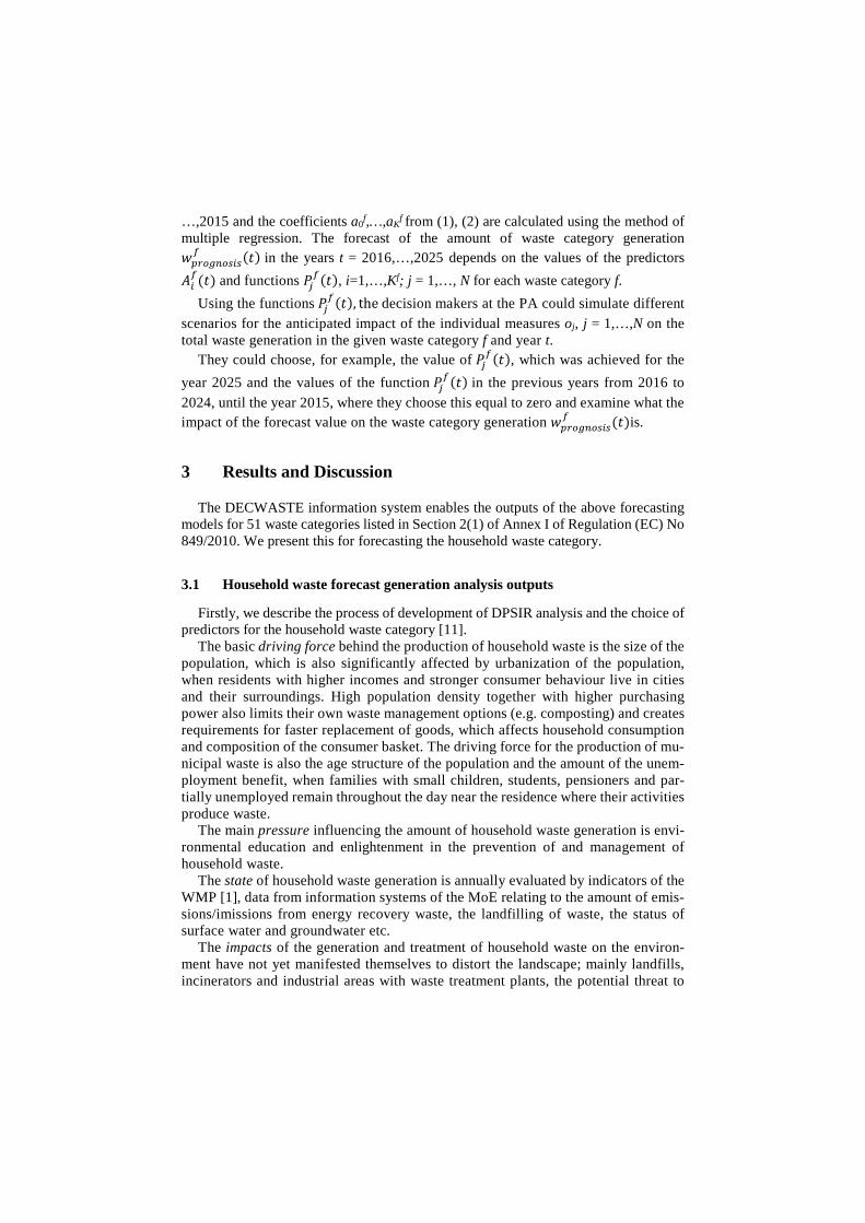
3 Results and Discussion

The DECWASTE information system enables the outputs of the above forecasting models for 51 waste categories listed in Section 2(1) of Annex I of Regulation (EC) No 849/2010. We present this for forecasting the household waste category.

3.1 Household waste forecast generation analysis outputs

Firstly, we describe the process of development of DPSIR analysis and the choice of predictors for the household waste category [11].

The basic driving force behind the production of household waste is the size of the population, which is also significantly affected by urbanization of the population, when residents with higher incomes and stronger consumer behaviour live in cities and their surroundings. High population density together with higher purchasing power also limits their own waste management options (e.g. composting) and creates requirements for faster replacement of goods, which affects household consumption and composition of the consumer basket. The driving force for the production of mu-nicipal waste is also the age structure of the population and the amount of the unem-ployment benefit, when families with small children, students, pensioners and par-tially unemployed remain throughout the day near the residence where their activities produce waste.

The main pressure influencing the amount of household waste generation is envi-ronmental education and enlightenment in the prevention of and management of household waste.

The state of household waste generation is annually evaluated by indicators of the WMP [1], data from information systems of the MoE relating to the amount of emis-sions/imissions from energy recovery waste, the landfilling of waste, the status of surface water and groundwater etc.

The impacts of the generation and treatment of household waste on the environ-ment have not yet manifested themselves to distort the landscape; mainly landfills, incinerators and industrial areas with waste treatment plants, the potential threat to

groundwater and surface water and air pollution, etc. Furthermore, collection and transport of household waste and pollution in the case of collection containers, etc.

The response to generated household waste is increasing the number of collection places for sorting waste and streamlining the system of collection and treatment of household waste. There is, along with improving municipal waste management sys-tems, the education of the population in the context of environmental education. To-gether with education legislative measures are used, which are operated both by the municipality as the originator of household waste, so the whole system for the col-lection and processing of waste, i.e. throughout the life cycle of the household waste. Legislative instruments are accompanied by economic instruments, in the form of charges (waste disposal in a landfill), and the amount of the tax rates and subsidies directed towards the development of systems for the municipal waste management.

The expert group choose the most significant four predictors for household waste for which past time series are available or can be estimated [11]:

• Driving forces: population; number of retired; unemployed rate; household expendi-ture on food, footwear and clothing.

• Press: prevention percentage according to environmental awareness (sorting rate, influence of ecological education etc.) which decreases the amount of household waste.

• State: household waste generation.

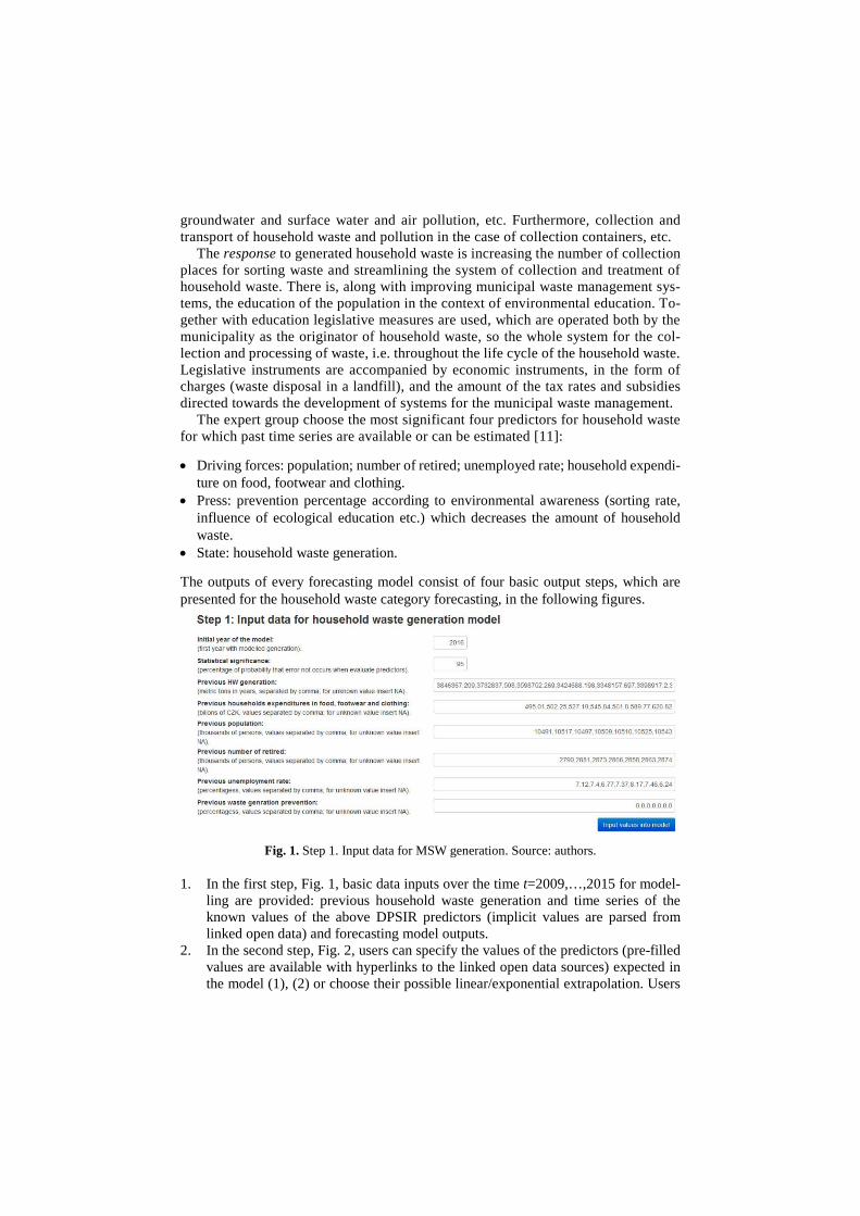
The outputs of every forecasting model consist of four basic output steps, which are presented for the household waste category forecasting, in the following figures.

Fig. 1. Step 1. Input data for MSW generation. Source: authors.

1. In the first step, Fig. 1, basic data inputs over the time t=2009,…,2015 for model-ling are provided: previous household waste generation and time series of the known values of the above DPSIR predictors (implicit values are parsed from linked open data) and forecasting model outputs.

2. In the second step, Fig. 2, users can specify the values of the predictors (pre-filled values are available with hyperlinks to the linked open data sources) expected in the model (1), (2) or choose their possible linear/exponential extrapolation. Users

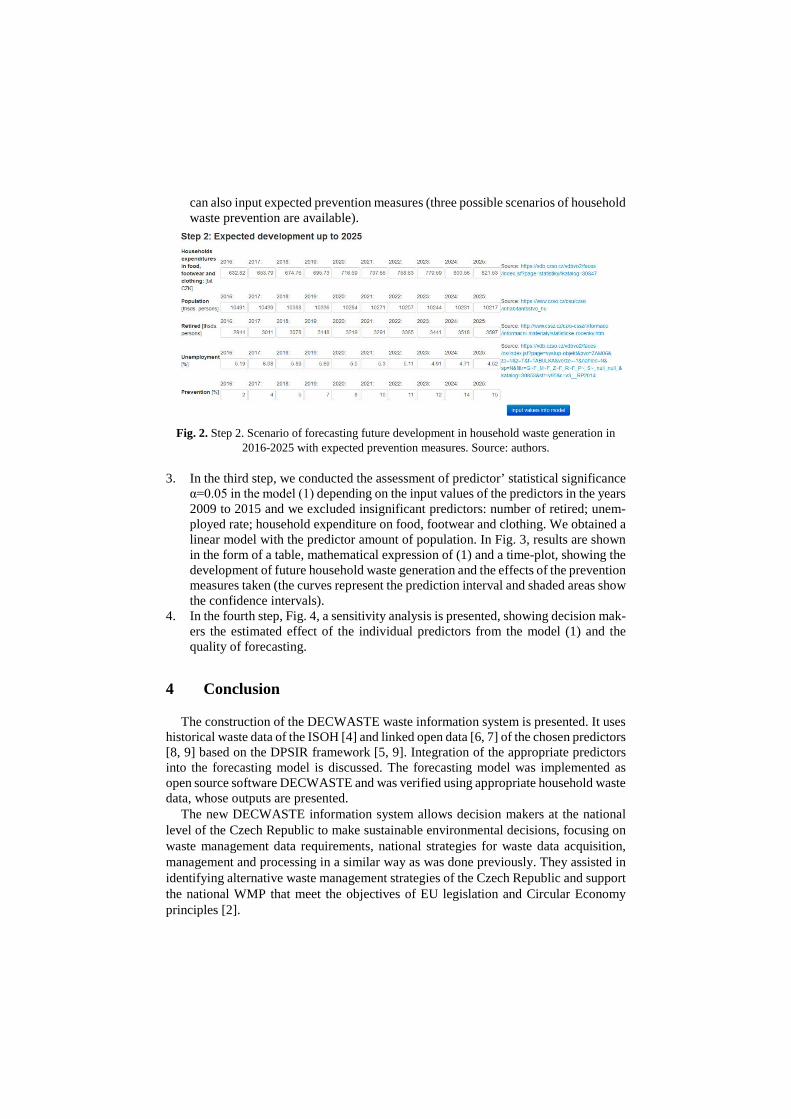
can also input expected prevention measures (three possible scenarios of household waste prevention are available).

Fig. 2. Step 2. Scenario of forecasting future development in household waste generation in

2016-2025 with expected prevention measures. Source: authors.

3. In the third step, we conducted the assessment of predictor’ statistical significance α=0.05 in the model (1) depending on the input values of the predictors in the years 2009 to 2015 and we excluded insignificant predictors: number of retired; unem-ployed rate; household expenditure on food, footwear and clothing. We obtained a linear model with the predictor amount of population. In Fig. 3, results are shown in the form of a table, mathematical expression of (1) and a time-plot, showing the development of future household waste generation and the effects of the prevention measures taken (the curves represent the prediction interval and shaded areas show the confidence intervals).

4. In the fourth step, Fig. 4, a sensitivity analysis is presented, showing decision mak-ers the estimated effect of the individual predictors from the model (1) and the quality of forecasting.

4 Conclusion

The construction of the DECWASTE waste information system is presented. It uses historical waste data of the ISOH [4] and linked open data [6, 7] of the chosen predictors [8, 9] based on the DPSIR framework [5, 9]. Integration of the appropriate predictors into the forecasting model is discussed. The forecasting model was implemented as open source software DECWASTE and was verified using appropriate household waste data, whose outputs are presented.

The new DECWASTE information system allows decision makers at the national level of the Czech Republic to make sustainable environmental decisions, focusing on waste management data requirements, national strategies for waste data acquisition, management and processing in a similar way as was done previously. They assisted in identifying alternative waste management strategies of the Czech Republic and support the national WMP that meet the objectives of EU legislation and Circular Economy principles [2].

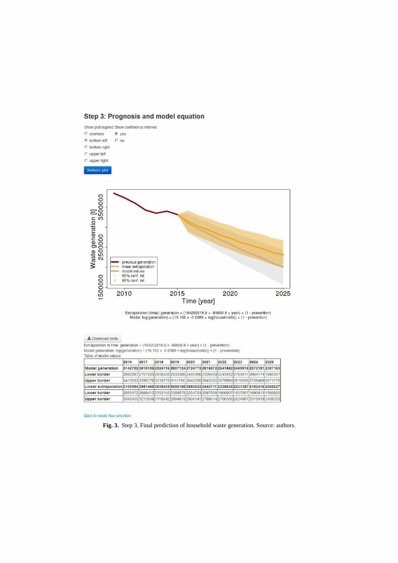
Fig. 3. Step 3. Final prediction of household waste generation. Source: authors.

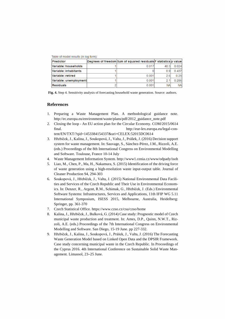
Fig. 4. Step 4. Sensitivity analysis of forecasting household waste generation. Source: authors.

References

1. Preparing a Waste Management Plan. A methodological guidance note. http://ec.europa.eu/environment/waste/plans/pdf/2012_guidance_note.pdf

2. Closing the loop - An EU action plan for the Circular Economy. COM/2015/0614 final. http://eur-lex.europa.eu/legal-con-tent/EN/TXT/?qid=1453384154337&uri=CELEX:52015DC0614

3. Hřebíček, J., Kalina, J., Soukopová, J., Valta, J., Prášek, J. (2016) Decision support system for waste management. In: Sauvage, S., Sánchez-Pérez, J.M., Rizzoli, A.E. (eds.) Proceedings of the 8th International Congress on Environmental Modelling and Software. Toulouse, France 10-14 July

4. Waste Management Information System. http://www1.cenia.cz/www/odpady/isoh 5. Liao, M., Chen, P., Ma, H., Nakamura, S. (2015) Identification of the driving force

of waste generation using a high-resolution waste input-output table. Journal of Cleaner Production 94, 294-303

6. Soukopová, J., Hřebíček, J., Valta, J. (2015) National Environmental Data Facili-ties and Services of the Czech Republic and Their Use in Environmental Econom-ics. In: Denzer, R., Argent, R.M., Schimak, G., Hřebíček, J. (Eds.) Environmental Software Systems: Infrastructures, Services and Applications, 11th IFIP WG 5.11 International Symposium, ISESS 2015, Melbourne, Australia, Heidelberg: Springer, pp. 361-370

7. Czech Statistical Office. https://www.czso.cz/csu/czso/home 8. Kalina, J., Hřebíček, J., Bulková, G. (2014) Case study: Prognostic model of Czech

municipal waste production and treatment. In: Ames, D.P., Quinn, N.W.T., Riz-zoli, A.E. (eds.) Proceedings of the 7th International Congress on Environmental Modelling and Software. San Diego, 15-19 June. pp 227-332.

9. Hřebíček, J., Kalina, J., Soukopová, J., Prášek, J., Valta, J. (2016) The Forecasting Waste Generation Model based on Linked Open Data and the DPSIR Framework. Case study concerning municipal waste in the Czech Republic. In Proceedings of the Cyprus 2016. 4th International Conference on Sustainable Solid Waste Man-agement. Limassol, 23–25 June.

10. Seker, S.E. (2015) Computerized Argument Delphi Technique. IEEE Access. 3, 368–380. doi:10.1109/ACCESS.2015.2424703

11. Horáková, E., Kalina, J., Hřebíček, J., Prášek, J., Soukopová, J., Buda Šepeľová, G., Valta, J. (2015) Vyhodnocení DPSIR rámce pro vybrané skupiny odpadů stano-vené výzvou TB940MZP003. (Evaluation of the DPSIR framework for selected groups of waste laid down a challenge TB940MZP003). Internal report. CENIA, Praha