Modelling and Management of Mortality Risk: A Revie · will be considerable uncertainty in forecasting what rates of improvement will be in ... The modelling and management of systematic

1

Modelling and Management of Mortality Risk:A Review

Andrew J.G. CairnsDavid BlakeKevin Dowd

First version: December 2007This version: May 22, 2008

Abstract

In the first part of the paper, we consider the wide range of extrapolative stochasticmortality models that have been proposed over the last 15 to 20 years. A numberof models that we consider are framed in discrete time and place emphasis on thestatistical aspects of modelling and forecasting. We discuss how these models can beevaluated, compared and contrasted. We also discuss a discrete-time market modelthat facilitates valuation of mortality-linked contracts with embedded options. Wethen review several approaches to modelling mortality in continuous time. Thesemodels tend to be simpler in nature, but make it possible to examine the potentialfor dynamic hedging of mortality risk. Finally, we review a range of financial in-struments (traded and over-the-counter) that could be used to hedge mortality andrisk. Some of these, such as mortality swaps, already exist, while others anticipatefuture developments in the market.

Keywords: stochastic mortality models, short-rate models, market models, cohorteffect, SCOR market model, mortality-linked securities, mortality swaps, q-forwards.

1 INTRODUCTION 2

1 Introduction

The twentieth century has seen significant improvements in mortality rates. Figure1 demonstrates this for selected ages for English and Welsh males. To facilitateunderstanding, these rates have been plotted on a logarithmic scale, and with thesame relative range of values on the vertical axis (that is, the maximum on each scaleis 12 times the minimum). From these plots we can extract the following stylisedfacts which apply to most developed countries (for example, Western Europe, Scan-dinavia, North America):

• Mortality rates have fallen dramatically at all ages.

• At specific ages, improvement rates seem to have varied over time with sig-nificant improvements in some decades and almost no improvements in otherdecades. For example, for English and Welsh males, the age 25 rate improveddramatically before 1960 and then levelled off; at age 65 the opposite was true.

• Improvement rates have been significantly different at different ages. For ex-ample, for English and Welsh males, the age 45 improvements have been muchhigher than the age 85 improvements.

• Aggregate mortality rates reveal significant volatility from one year to thenext. This is especially true at both young ages, where the numbers of deathsare relatively small, and high ages. At high ages, the numbers of deaths are,of course, high, so we infer that there are genuine annual fluctuations in thetrue underlying rates of mortality at high ages. These fluctuations might,for example, be due to the incidence of winter flu epidemics or summer heatwaves in some years causing increased mortality amongst the old and frail inthe population in those years.

From a statistical perspective, we might also add a further point. Since rates ofimprovement have varied over time and have been different at different ages, therewill be considerable uncertainty in forecasting what rates of improvement will be inthe future at different ages.

In some, but not all countries, an additional observation has been made that pat-terns of improvement are linked to year of birth (see, for example, Willets, 2004,and Richards et al., 2006). In Figure 2, we have plotted 5-year-average rates ofimprovement (that is, −0.2 log[q(t, x)/q(t− 5, x)], where q(t, x) is the mortality rateat age x in year t). In this plot, we can see that there are clear groupings of highimprovement rates and of low improvement rates. We have specifically highlightedthe cohort born around 1930 by a solid black diagonal line. The shading alongthis diagonal is clearly lighter than other diagonals indicating that individuals bornaround that time (1925 to 1935) have experienced rather larger improvements in

1 INTRODUCTION 3

1900 1940 1980

0.00

10.

002

0.00

4

Age = 25

Year

Mor

talit

y ra

te

1900 1940 1980

0.00

50.

010

0.02

0

Age = 45

Year

Mor

talit

y ra

te

1900 1940 1980

0.05

0.10

Age = 65

Year

Mor

talit

y ra

te

1900 1940 1980

0.2

0.4

0.8

Age = 85

Year

Mor

talit

y ra

te

Figure 1: England and Wales males: Mortality rates at ages 25, 45, 65 and 85.Rates are plotted on a logarithmic scale, with the same relative range of values ineach plot. The age-25 rate for 1918 is off the scale.

1 INTRODUCTION 4

1970 1980 1990 2000

2040

6080

Year

Age

−2%

−1%

0%

1%

2%

3%

4%

Ann

ual i

mpr

ovem

ent r

ate

(%)

Figure 2: Improvement rates in mortality for England & Wales by calendar yearand age relative to mortality rates at the same age in the previous year. Black cellsimply that mortality is deteriorating; medium grey small rates of improvement, andwhite strong rates of improvement. The black diagonal line follows the progress ofthe 1930 cohort. (Source: Cairns et al., 2007)

mortality compared with people born before or after. Possible explanations for this‘golden’ cohort include a healthy diet in the 1940’s and early 1950’s (or, to be moreprecise, shortages of unhealthy food), and the introduction of the National HealthService. In more general terms, it is easy to detect diagonals above age 30 runningthrough Figure 2, and this is indicative of year of birth potentially being an impor-tant factor in projecting future mortality rates for England and Wales males. Alsoin Figure 2, we can see: strong reductions in mortality amongst the very young; anda deterioration in mortality amongst males in their 20’s during the late 1980’s and1990’s (due to the AIDS epidemic).

1.1 Systematic and unsystematic mortality

It is appropriate at this point to discuss mortality in a more scientific setting. Wewill define q(t, x) to be the underlying aggregate mortality rate in year t at age x.This is an unobservable rate. What we do observe depends on how, for example,

1 INTRODUCTION 5

national statistics offices record deaths and population sizes. However, in manycountries we observe the crude death rate, mc(t, x), which is the number of deaths,D(t, x), aged x last birthday at the date of death, during year t, divided by theexposure, E(t, x) (the average population aged x last birthday during year t).1

The uncertainty in future death rates can be divided into two components:

• Unsystematic mortality risk: even if the true mortality rate is known, thenumber of deaths, D(t, x), will be random. The larger is the population,the smaller is the unsystematic mortality risk (as a result of the pooling ofoffsetting risks, i.e., diversification).

• Systematic mortality risk: this is the undiversifiable component of mortalityrisk that affects all individuals in the same way. Specifically, forecasts ofmortality rates in future year are uncertain.

1.2 Life assurers and pension plans

The modelling and management of systematic mortality risk are two of the mainconcerns of large life assurers and pension plans and we will focus in this paper onthese two concerns:

• Modelling:

– what is the best way to forecast future mortality rates and to model theuncertainty surrounding these forecasts?

– how do we value risky future cashflows that depend on future mortalityrates?

• Management:

– how can this risk be actively managed and reduced as part of an overallstrategy of efficient risk management?

– what hedging instruments are easier to price than others?

In order to address these questions, we require the following: first, we need suitablestochastic mortality models capable of forecasting the distribution of future mortal-ity rates which will help with both quantifying and pricing mortality risk; second,we need suitable vehicles for managing or transferring mortality risk. In addition to

1In our notation the subscript c in mc(t, x) distinguishes the crude or actual death rate fromthe underlying or expected death rate.

2 BASIC BUILDING BLOCKS 6

focusing on these two requirements, we also review the rapidly developing literaturein this field, as well as present some new ideas and models.

In Section 2, we introduce some of the basic notation that is required in the subse-quent Sections 3 to 5 where we discuss specific approaches to modelling. In Section3.1, before looking at particular models, we review the range of criteria that can beused to evaluate different models. We then move on, in Sections 4 and 5, to discussdiscrete-time and continuous-time models. We develop some new insights as wellas some new models (including a new model with a cohort effect, a generalisationof the Olivier-Smith market model and further thoughts on the SCOR [survivorcredit offered rate] market model). Section 6 reviews existing and potential marketinstruments that might be used to help manage mortality risk. Section 7 concludes.

2 Basic building blocks

For modelling, we need to define some general notation.

2.1 Mortality rates

q(t, x) is the underlying probability that an individual aged exactly x at time t willdie before time t+1. The period t to t+1 will also be referred to as “year t”. q(t, x)is normally only defined for integer values of x and t, and is only observable aftertime t + 1.

2.2 The instantaneous force of mortality

µ(t, x) is the underlying force of mortality at time t and age x for real t and x.

We have the relationship

q(t, x) = 1− exp

[−

∫ t+1

t

µ(u, x− t + u)du

]

which we treat as being observable only after time t + 1.

2.3 The survivor index

The survivor index is defined as

S(t, x) = exp

[−

∫ t

0

µ(u, x + u)du

].


An informal way of thinking about S(t, x) is that it represents the proportion ofa large population aged exactly x at time 0 who survive to age x + t at time t.More formally, let Mt be the filtration generated by the whole of the instantaneousforce of mortality curve (that is, covering all ages) up to time t, so that S(t, x) isMt-measurable. Now consider a single individual aged exactly x at time 0. Let I(t)be the indicator random variable that is equal to 1 if the individual is still alive attime t and 0 if he is dead.

Then Pr[I(t) = 1|Mt] = S(t, x). Further, Pr[I(t) = 1|Mu] = S(t, x) for all u ≥ t.

Remark: (See, for example, Biffis et al., 2006) The filtration Mt informs us aboutthe underlying mortality dynamics only. It does not tell us about the times of deathof individuals in the population. We will denote by M∗

t the augmented filtrationthat is generated by both µ(t, x) and the times of death of the individuals in thepopulation.

2.4 Spot and forward survival probabilities

Our remark about u ≥ t in subsection 2.3 raises the question as to what happens ifu < t. For 0 < u < t,

Pr[I(t) = 1|Mu] = E[S(t, x)|Mu] = S(u, x)E

[S(t, x)

S(u, x)

∣∣∣∣Mu

].

This leads us to the definition of the spot survival probabilities:

p(u, t, x) = Pr[I(t) = 1|I(u) = 1,Mu]

so that Pr[I(t) = 1|Mu] = S(u, x)p(u, t, x).

Finally, this leads us to define forward survival probabilities for T0 < T1:

p(t, T0, T1, x) = Pr[I(T1) = 1|I(T0) = 1,Mt]. (1)

The name forward survival probability suggests that t ≤ T0, but, in fact, the prob-ability is well defined for any t.

Remark: It is important to keep in mind that the spot and forward survival proba-bilities, p(t, T, x) and p(t, T0, T1, x) concern individuals aged x at time 0 and not attime t.

2.5 Real-world and risk-neutral probabilities

In the remarks above, we have implicitly assumed that probabilities and expectationshave been calculated under the true or real-world probability measure, P . When


it comes to pricing, we will often use an artificial, risk-neutral probability measure,Q. The extent to which P and Q differ depends, for example, upon how much ofa premium life assurers and pension plans would be prepared to pay to hedge theirsystematic and possibly non-systematic mortality risks, giving rise to the concept ofa market price of risk.

Most previous research (see, for example, Cairns et al., 2006a, and references therein)assumes that there is a market price of risk for systematic mortality risk only andthat non-systematic risk, being diversifiable, goes unrewarded. Under this assump-tion

PrQ[I(t) = 1|Mt] = PrP [I(t) = 1|Mt] = S(t, x)

but, for u < t, PrQ[I(t) = 1|Mu] and PrP [I(t) = 1|Mu] are not necessarily equal.

With an illiquid market, it is, nevertheless, plausible that insurers might be preparedto pay a premium to hedge their exposure to non-systematic mortality risk, inthe same way that individuals are prepared to pay insurers a premium above theactuarially fair (i.e. P ) price of an annuity in order to insure against their personallongevity risk. Under these circumstances, we need to define a risk-neutral force ofmortality µQ(t, x) and the corresponding risk-neutral survivor index

S(t, x) = exp

[−

∫ t

0

µ(u, x + u)du

].

Then PrQ[I(t) = 1|Mt] = S(t, x). The concept of a non-zero market price of riskfor non-systematic mortality risk is explored further by Biffis et al. (2006).

Similarly, most modelling of stochastic mortality has assumed that the dynamics ofthe force of mortality curve are independent of the evolution of the term structureof interest rates. Under these circumstances, the value at time t of a pure mortality-linked cashflow X at a fixed time T can be written as the product of the zero-couponbond price P (t, T ) and the risk-neutral expected value of X given the informationavailable at time t.

2.6 Zero-coupon fixed-income and longevity bonds

In what follows, we wish to consider the value of mortality-linked cashflows. To dothis, we need to introduce two types of financial asset: zero-coupon fixed-incomebonds, and zero-coupon longevity bonds.

The time T -maturity zero-coupon bond pays a fixed amount of 1 unit at time T . Theprice at time t of this bond is denoted by P (t, T ). We will assume that underlyinginterest rates are stochastic, and the reader is referred to Cairns (2004) or Brigo andMercurio (2001) for textbook accounts of interest rate models. Also relevant hereis a cash account C(t) that constantly reinvests at the (stochastic) instantaneousrisk-free rate of interest, r(t), so that C(t) = exp[

∫ t

0r(u)du].


Zero-coupon longevity bonds (or zero-coupon survivor bonds, as Blake and Burrows,2001, originally called them) can take two forms. Each type is characterised by amaturity date, T , and a reference cohort aged x at time 0, and we will refer to thisas the (T, x)-longevity bond. Type A pays S(T, x) at time T and the market valueat time t of this bond will be denoted by BS(t, T, x). Type B pays C(T )S(T, x) attime T , and the market value at time t of this bond will be denoted by BCS(t, T, x).

Throughout the rest of this paper, we will, for simplicity of exposition, assume thatthe term structure of interest rates is independent of the term structure of mortality,and that the market price of risk for non-systematic mortality risk is zero. It followsthat (see, for example, Cairns et al., 2006a)

BS(t, T, x) =P (t, T )BCS(t, T, x)

C(t).

Prices are linked to an artificial risk-neutral pricing measure Q (see above) as follows(see Cairns et al, 2006a)

BCS(t, T, x) = EQ

[C(t)

C(T )C(T )S(T, x)

∣∣∣∣Ht

]= C(t)EQ[S(T, x)|Mt]. (2)

Here, Ht represents the augmented filtration that includes information about bothmortality and interest rates up to time t.

Remark: (Fundamental Theorem of Asset Pricing) If there exists such a risk-neutral measure Q, and if prices are calculated according to equation (2), then themarket will be arbitrage free. This includes markets that are incomplete or illiquid.

It follows that BCS(t, T, x) = C(t)S(t, x)pQ(t, T, x), where pQ(t, T, x) is the risk-neutral spot survival probability, EQ[S(T, x)/S(t, x)|Mt]. This represents the risk-adjusted probability, based on the information available at time t, that an individualaged x + t at t will survive until age x + T .

2.6.1 Risk-neutral spot and forward survival probabilities

If the spot market in type-B bonds is sufficiently liquid for a range of maturities,then we can take as given the bond prices, BCS(t, T, x), at time t. This then definesthe risk-neutral spot survival probabilities

pQ(t, T, x) =BCS(t, T, x)

C(t)S(t, x)

from which we can define the risk-neutral forward survival probabilities

pQ(t, T0, T1, x) = pQ(t, T1, x)/pQ(t, T0, x) for t ≤ T0

and pQ(t, T0, T1, x) =S(t, x)

S(T0, x)pQ(t, T1, x) for t > T0. (3)

3 STOCHASTIC MORTALITY MODELS: INTRODUCTORY REMARKS 10

2.6.2 The forward mortality surface

In the traditional mortality setting, with no mortality improvements, the force ofmortality can be defined as µx+t = −∂ log tpx/∂t. In the current context, this canbe developed as a concept for individual cohorts. We assume for a given cohort agedx at time 0 that the spot survival probabilities, pQ(t, T, x), are known at time t forall T > 0 (not just integer values of T ). The forward force of mortality surface (or,more simply, forward mortality surface) is defined as (see Dahl, 2004)

µ(t, T, x + T ) = − ∂

∂Tlog pQ(t, T, x). (4)

At a given time t, this defines a two-dimensional surface in age, x, and maturity,T . It can be regarded as a central estimate, based on information available at timet, of the force of mortality at the future time T (that is, T − t years ahead) forindividuals aged x + T at time T .

3 Stochastic mortality models: Introductory re-

marks

In Sections 3.1 to 5, we will review the full range of approaches that can be takento modelling future randomness in mortality rates.

At least in theory (published modelling work has still to fill some gaps), there is awide range of extrapolative approaches that can be taken to model mortality. Somemodels are framed in discrete time, others in continuous time. In discrete time, mostresearch has focused on the statistical analysis and projection of annual mortalitydata using what will be described below as short-rate models. However, some workhas also been done using P-splines and discrete-time market models. In continuoustime, most research has also focused on short-rate models including affine mortalitymodels. But other approaches analogous to forward-rate models and market modelsin interest-rate modelling have also been proposed or discussed.

3.1 Model selection criteria

Once a model has been developed and parameters have been estimated or calibrated,it is important to consider whether it is a good model or not. This requires a check-list of criteria against which a model can be assessed, along the lines proposed byCairns, Blake and Dowd (2006a) and Cairns et al. (2007, 2008):

• Mortality rates should be positive.


• The model should be consistent with historical data.

• Long-term dynamics under the model should be biologically reasonable.

• Parameter estimates should be robust relative to the period of data and rangeof ages employed.

• Model forecasts should be robust relative to the period of data and range ofages employed.

• Forecast levels of uncertainty and central trajectories should be plausible andconsistent with historical trends and variability in mortality data.

• The model should be straightforward to implement using analytical methodsor fast numerical algorithms.

• The model should be relatively parsimonious.

• It should be possible to use the model to generate sample paths and calculateprediction intervals.

• The structure of the model should make it possible to incorporate parameteruncertainty in simulations.

• At least for some countries, the model should incorporate a stochastic cohorteffect.

• The model should have a non-trivial correlation structure.

Some of these points require further comment to bring out their relevance.

3.2 Consistency with historical data

At a minimum, a good model should be consistent with historical patterns of mor-tality. If this is not the case, much greater doubt must be placed on the validity ofany forecasts produced by the model.

More formal statistical approaches have been used by, for example, Brouhns, Denuitand Vermund (2002) and Czado, Delvarde and Denuit (2005), using full likelihoodmethods and Markov Chain Monte Carlo (MCMC) methods. Additionally, Cairns etal. (2007) carried out a detailed comparison of different models based on maximumlikelihoods, using criteria that penalise over-parameterised models. They showedthat statistically significant improvements on the Lee and Carter (1992) and Cairns,Blake and Dowd (2006b) models can be achieved by adding extra period and cohorteffects. They also demonstrated that the fundamental assumption under these sim-ple models that the two-dimensional array of standardised residuals be independent


and identically distributed is violated, thereby calling into question their consistencywith historical data. Further historical analysis has been performed by Dowd et al.(2008a,b) who use a variety of backtesting procedures to evaluate out-of-sampleperformance of a range of models.

3.3 Biological reasonableness

Cairns et al. (2006a) introduce the concept of biological reasonableness, drawingon the concept of economic reasonableness from interest-rate modelling. Differentmodellers might have their own idea about what constitutes a biologically reasonablemodel, but we offer the following examples of what might be considered biologicallyunreasonable:

• Period mortality tables have historically exhibited increasing rates of mortalitywith age at higher ages. A forecasting model that gives rise to the possibilityof period mortality tables that have mortality rates falling with age might beconsidered biologically unreasonable.

• Short-term mean reversion might be considered to be biologically reasonabledue to annual environmental variation. Long-run mean reversion around adeterministic trend might, on the other hand, be considered biologically un-reasonable. In the long term, mortality improvements will, amongst otherreasons, be the result of medical advances, such as a cure for cancer. It is verydifficult to predict when such advances will happen or what the impact of anew treatment might be. A deterministic mean-reversion level would suggestthat we do know what advances are going to happen and what their impactwill be: we just do not know when they will happen.

3.4 Robustness of parameter estimates and forecasts

When we fit a model, we need to specify what range of ages and past years wewill use to estimate parameters: for example, ages 60 to 89, and years 1960 to2005. Ultimately, we wish to have confidence in the forecasts that are produced bya model. With most models, we find that a change in the range of years or of ages inthe historical dataset results in a relatively modest revision of parameter estimates,consistent with the statistical variation in the data. Such models might be describedas being robust.

For other models, however, a change in the age or calendar-year range sometimesresults in (a) a set of qualitatively different parameter estimates and (b) substantiallydifferent forecasts of future mortality. Such models are not robust and they cannotbe relied upon to produce consistently reasonable forecasts.


3.5 Plausibility of forecasts

The plausibility of forecasts is again a rather subjective issue, discussed by Cairnset al. (2008). In general, one cannot normally make a definitive statement that aset of forecasts look reasonable. However, Cairns et al. (2008) do provide examplesof models that provide a statistically good fit to the historical data, but then pro-duce quite implausible projections of mortality. Examples, of implausible forecastsinclude: a sudden and dramatic change in the central trend in mortality rates atcertain ages; and prediction intervals for mortality that are either extremely wideor extremely narrow.

3.6 Implementation

There is little point in having a great model if it requires excessive amounts ofcomputing time to calculate important quantities of interest. If this happens, thena compromise needs to be reached, ideally without sacrificing too much in terms ofstatistical goodness of fit.

3.7 Parsimony

We should avoid models that are excessively parameterised. This can be addressedby using, for example, the Bayes Information Criterion (BIC), to choose betweenmodels. This ensures that extra parameters are only included when there is asignificant improvement in fit.

3.8 Sample paths and prediction intervals

Most models (except for P-splines models) generate sample paths and thereforeallow an assessment of the uncertainty in future mortality-linked cashflows, andthe pricing of these cashflows. Pricing might require a change of measure and thisrequires a fully specified stochastic model with sample paths.

3.9 Parameter uncertainty

We have a limited amount of data that we can use to estimate model parameters,and so it follows that these parameters will be subject to estimation error. It isimportant to be able to incorporate parameter uncertainty, if we wish, into simula-tions in order to assess the impact of this estimation error. Cairns et al. (2006b)and, for example, Dowd et al. (2007) investigated this issue in the Cairns-Blake-Dowd two-factor model and found that the inclusion of parameter uncertainty has a

4 DISCRETE-TIME MODELS 14

significant impact on forecast levels of uncertainty in mortality rates and expectedfuture lifetimes, especially at longer time horizons. We do not discuss the issue ofparameter uncertainty further in this paper, but note that this, along with modelrisk, are important issues that require substantial further research.

3.10 Cohort effect

As remarked earlier, some countries including England and Wales, have mortalityrates that appear to be determined not just by age and period effects but also byyear-of-birth effects. Cairns et al. (2007) demonstrated that the inclusion of acohort effect provided a statistically significantly better fit. We would expect thatsuch effects will persist into the future and that forecasts will, therefore, be improvedby the inclusion of a cohort effect.

3.11 Correlation term structure

As also remarked earlier in this paper and elsewhere, rates of improvement at differ-ent ages have been different both over long periods of time and also from one yearto the next. In other words, improvements at different ages might be correlated, butthey are not perfectly correlated. The use of a model that assumes perfect correla-tion might cause problems for two reasons. First, aggregate levels of uncertainty atthe portfolio level might be overstated (since it is assumed that there are no diversi-fication benefits across ages). Second, perfect correlation would incorrectly suggestthat derivative instruments linked to mortality at one age could be used to hedgeperfectly mortality improvements at a different age. Ignoring this problem mightresult in a degree of hidden basis risk if hedging stratgies are adopted that rely onperfect correlation.

4 Discrete-time models

National mortality data are generally published on an annual basis and by individualyear of age, and this leads naturally to the development of discrete-time models.Typically, the data are presented in the form of crude death rates

mc(t, x) =D(t, x)

E(t, x)=

#deaths during calendar year t aged x last birthday

average population during calendar year t aged x last birthday.

The average population (the exposure) will normally be an approximation, eitherbased on a mid-year population estimate or on estimates of the population at thestart and end of each year. Cairns et al. (2007) found, for example, that USexposures data tended to be rather less reliable than England and Wales data,


leading to less reliable parameter estimates for stochastic mortality models.2 Thenumbers of deaths are usually felt to be known with greater accuracy, although theaccuracy might depend on local laws concerning the reporting of deaths.

Some authors have chosen to model the death rates directly, while others choose tomodel mortality rates, q(t, x), the underlying probability that an individual agedexactly x at time t will survive until time t + 1.

The two are linked, typically, by one of two approximations: q(t, x) = 1−exp[−m(t, x)];or q(t, x) = m(t, x)/(1 + 0.5m(t, x)).

4.1 The Lee-Carter model

The availability of annual data subdivided into integer ages means that it is relativelystraightforward to use rigorous statistical methods to fit discrete-time models to thedata. This has tended to produce models that are straightforward to simulate indiscrete time but which do not lead to analytical formulae for, for example, spotsurvival probabilities.

The earliest model and still the most popular is the Lee and Carter (1992) model

m(t, x) = exp[β(1)

x + β(2)x κ

(2)t

]

where the β(k)x are age effects and κ

(2)t is a random period effect. Under this model,

β(1)x represents an average log mortality rate over time at age x, while β

(2)x represents

the improvement rate at age x. The period effect, κ(2)t , is often modelled as a random-

walk process (e.g. Lee and Carter, 1992) or as an ARIMA process (e.g. CMI, 2007).

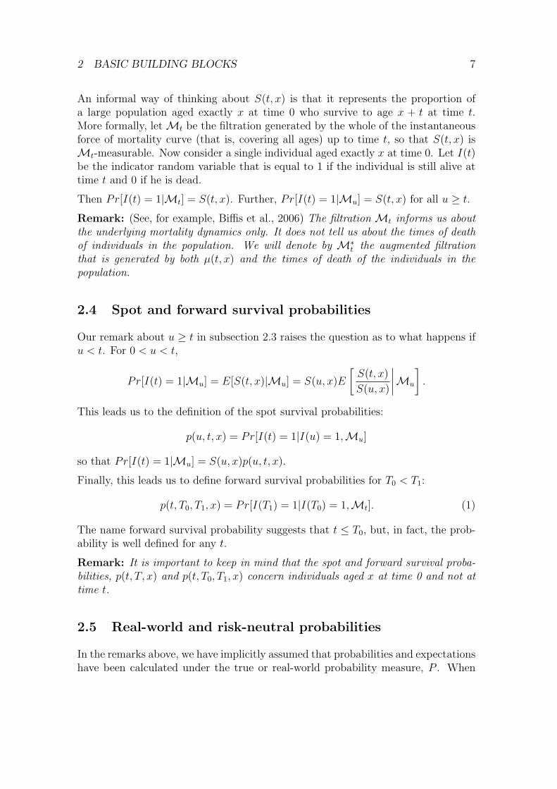
A variety of approaches have been taken to the estimation of parameters. The earlyapproach of Lee and Carter has been largely replaced by more formal statisticalmethods (Brouhns et al, 2002, Czado et al., 2005, and Delwarde at al., 2007) withthe primary focus on goodness of fit over all of the data. A rather different approachwas taken by Lee and Miller (2001) who took the view that a greater emphasis oughtto be placed on goodness of fit in the final year in the dataset. They observed thatthe purpose of modelling is normally to project mortality rates. However, the usualstatistical procedures aim to fit the historical data well over all past years. Thismeans that the final year of historical data (sometimes referred to as the stepping-off year) might have a relatively poor fit. (Note also, that this problem tends tobe worse if more calendar years of data are used.) As an example, Figure 3 showsestimated underlying mortality rates in 2004 for England and Wales mortality data(1961 to 2004, and ages 60 to 89) using the Lee-Carter model. We can see that thefitted curve systematically underestimates the death rate at lower ages. Based on

2To date, we are unaware of any studies that have explicitly attempted to model the exposuresas unobserved variables.


an out-of-sample analysis, Lee and Miller (2001) observed that systematic bias ofthis type in the stepping-off year persists and it results in biased predictions of keyoutputs such as mortality rates at specific ages or of period life expectancy. To avoidthis problem, they suggested that β

(1)x should be calibrated to log death rates in the

stepping-off year, t0 (that is, β(1)x = log mc(t0, x)) in combination with κ

(2)t0 = 0.

Elsewhere in this paper, we will draw on interest rate modelling analogies. In thepresent context, we can liken the Lee-Miller method of calibrating rates againstthe stepping-off-year crude death rates to the Hull and White (1990) extension ofthe Vasicek (1977) interest rate model. The Vasicek model assumes a constantmean reversion level for interest rates, whereas the Hull and White model assumesa deterministic but time-varying mean-reversion level that is calibrated in a waythat ensures that theoretical zero-coupon bond prices match observed prices at timezero.

Other authors have adapted the methodology in an attempt to improve the modelfor κ

(2)t . The motivation for this (see, for example, Booth et al., 2002) is that the

drift of the random walk appears to change from time to time. De Jong and Tickle(2006) tackled this by modelling the drift itself as a latent random process. Onthe other hand, Booth et al. (2002) attempted to estimate the optimal estimationperiod for the random-walk model with constant drift. However, Booth et al.’smethod might lead to systematic underestimation of the true level of volatility inκ

(2)t .

The Lee-Carter model serves a useful pedagogical purpose, but the model has draw-backs:

• It is a one-factor model, resulting in mortality improvements at all ages beingperfectly correlated.

• The β(2)x age effect is normally measured as the average improvement rate at

age x, but β(2)x has a second purpose in setting the level of uncertainty in

future death rates at age x: V ar[log m(T, x)|Mt] = β(2)x

2V ar[κ

(2)T |κ(2)

t ]. Thismeans that uncertainty in future mortality rates cannot be decoupled fromimprovement rates. Historically, improvement rates have been lower at highages. This, in turn, means that predicted uncertainty in future death rateswill be significantly lower at high ages. However, this prediction does notconform with the high level of variability in mortality improvements at highages observed in historical data, undermining the validity of the model.

• Use of the basic version of the Lee-Carter model can result in a lack of smooth-ness in the estimated age effect, β

(2)x . Suppose that β

(1)x and β

(2)x have been

estimated using data up to, say, 1980. We can then carry out an out-of-sampleexperiment by taking β

(1)x and β

(2)x as given and estimating κ

(2)t for each fu-

ture year. We next calculate the standardised residuals for the out-of sample


60 65 70 75 80 85 90

−5.

0−

4.5

−4.

0−

3.5

−3.

0−

2.5

−2.

0−

1.5

Age

log

Dea

th R

ate

Figure 3: England and Wales males: log death rates in 2004 for ages 60 to 89. Dots:crude death rates. Solid line: Lee and Carter fitted curve of the underlying deathrate based on data from 1961 to 2004 and ages 60 to 89.


period, ε(t, x) = (D(t, x)−m(t, x)E(t, x)) /√

m(t, x)E(t, x). If the model andestimation method are correct, then the ε(t, x) should be independent andidentically distributed and approximately standard normal. Preliminary ex-periments indicate that if there is a lack of smoothness in β

(2)x , then there is a

clear inverse relationship between the β(2)x , for each x, and the observed out-

of-sample variance of the ε(t, x). This observation violates the i.i.d. standardnormality assumption.

Delwarde et al. (2007) tackle this problem by applying P-splines (see below)to the age effects.

• The problem of bias in forecasts identified by Lee and Miller (2001) and theirproposed solution arises fundamentally because the Lee-Carter model does notfit the data well. At a visual level, this is borne out by a plot of standardisedresiduals. The statistical approach proposed by Brouhns et al. (2002) assumesthat deaths, D(t, x), are independent Poisson random variables with mean and

variance both equal to m(t, x)E(t, x) where m(t, x) = exp[β(1)x +β

(2)x κ

(2)t ]. The

standardised residuals are

ε(t, x) = (D(t, x)−m(t, x)E(t, x))/√

m(t, x)E(t, x)).

Standardised residuals for England and Wales males are plotted in Figure4. If the residuals were independent then there should be no evidence ofclustering. However, Figure 4 shows clear evidence of clustering that violatethis assumption, especially along the diagonals (the so-called cohort effectidentified by Willets, 2004).

The Lee and Miller adjustment is therefore simply a ‘quick fix’ that improvesthe short-term problem of bias in forecasts. However, if the ‘usual’ method ofestimation (for example, Brouhns et al, 2002) has poor in-sample statisticalproperties, then the Lee-Miller calibration of the model will have the sameproblems with the reliability of long-term forecasts of mortality improvements.

4.2 Multifactor age-period models

A small number of multifactor models have appeared in recent years. As examples,Renshaw and Haberman (2003) propose the model

log m(t, x) = β(1)x + β(2)

x κ(2)t + β(3)

x κ(3)t

where κ(2)t and κ

(3)t are dependent period effects (for example, a bivariate random

walk).

Cairns, Blake and Dowd (2006b) focus on higher ages (60 to 89) and used therelatively simple pattern of mortality at these ages to fit a more parsimonious model


1970 1980 1990 2000

6065

7075

8085

90

Year

Age

Figure 4: England and Wales males: Standardised residuals, ε(t, x), for the Lee-Carter model fitted to ages 60 to 89 and years 1961 to 2004. Black cells indicate anegative residual; grey cells indicate a positive residual; white cells were excludedfrom the analysis. (Source: Cairns et al., 2007)


based on the logistic transform of the mortality rate rather than the log of the deathrate:

logit q(t, x) = logq(t, x)

1− q(t, x)= κ

(1)t + κ

(2)t (x− x)

where (κ(1)t , κ

(2)t ) is assumed to be a bivariate random walk with drift. Their analysis

also includes a detailed account of how parameter uncertainty can be included insimulations using Bayesian methods.

Both models offer significant qualitative advantages over the Lee-Carter model.However, both still fail to tackle the cohort effect.

4.3 The Renshaw-Haberman cohort model

Renshaw and Haberman (2006) proposed one of the first stochastic models for popu-lation mortality to incorporate a cohort effect (see also Osmond, 1985, and Jacobsenet al., 2002):

log m(t, x) = β(1)x + β(2)

x κ(2)t + β(3)

x γ(3)t−x

where κ(2)t is a random period effect and γ

(3)t−x is a random cohort effect that is a

function of the (approximate) year of birth, (t− x).

In their analysis of England and Wales males data, Renshaw and Haberman foundthat there was a significant improvement over the Lee-Carter model (see, also, Cairnset al., 2007). The most noticeable improvement was that an analysis of the stan-dardised residuals revealed very little dependence on the year of birth, in contrastwith the Lee-Carter model (see Figure 5). The upper plot (Lee-Carter) shows sig-nificant dependence on the year of birth, particularly between 1925 and 1935. Thecohort model (lower plot) shows no such dependence.

Unfortunately, the Renshaw-Haberman model turns out to suffer from a lack ofrobustness. CMI (2007) found that a change in the range of ages used to fit themodel might result in a qualitatively different set of parameter estimates. Cairnset al. (2007, 2008) found the same when they changed the range of years usedto fit the model. This lack of robustness is thought to be linked to the shape ofthe likelihood function. For robust models, the likelihood function probably has aunique maximum which remains broadly unchanged if the range of years or agesis changed. For models that lack robustness, the likelihood function possibly hasmore than one maximum. So when we change the age or year range, the optimiserwill periodically jump from one local maximum to another with qualitatively quitedifferent characteristics.

Cairns et al. (2008) note a further problem with the Renshaw-Haberman model.

The fitted cohort effect, γ(3)t−x, appears to have a deterministic linear, or possibly

quadratic, trend in the year of birth. This suggests that the age-cohort effect is


1880 1890 1900 1910 1920 1930 1940

−4

−2

02

4

Year of Birth

Res

idua

l

Lee−Carter Model

1880 1890 1900 1910 1920 1930 1940

−4

−2

02

4

Year of Birth

Res

idua

l

Renshaw−Haberman Cohort Model

Figure 5: England and Wales, males: Standardised residuals, ε(t, x), for the Lee-Carter and Renshaw-Haberman-cohort models. plotted against year of birth, t− x.Both models are fitted to ages 60 to 89 and years 1961 to 2004.


being used, inadvertently, to compensate for the lack of a second age-period effect,as well as trying to capture the cohort effect in the data. This suggests that animprovement on the model might be to combine the second age-period effect inRenshaw and Haberman (2003) with a simpler cohort effect. This might result in abetter fit, although it might not deal with the problem of robustness.

4.4 The Cairns-Blake-Dowd model with a cohort effect

Given the problems with the preceding models, a range of alternatives have beenexplored with the aim of finding a model that incorporates a parsimonious, multi-factor age-period structure with a cohort effect. Out of several models analysed, thefollowing generalisation of the Cairns-Blake-Dowd two-factor model (Cairns et al.,2006b) has been found to produce good results (see, also, Cairns et al., 2007):

logit q(t, x) = κ(1)t + κ

(2)t (x− x) + κ

(3)t

((x− x)2 − σ2

x

)+ γ

(4)t−x

where x = (xu − xl + 1)−1∑xu

x=xlx is the mean in the range of ages (xl to xu) to be

fitted, and σ2x = (xu − xl + 1)−1

∑xu

x=xl(x− x)2 is the corresponding variance.

Compared with the original model of Cairns et al. (2006b), there are two additional

components. First, there is an additional age-period effect, κ(3)t ((x− x)2 − σ2

x),that is quadratic in age. For both England and Wales and US males mortality data,this additional term was found to provide a statistically significant improvement,although it is considerably less important than the first two age-period effects. Sec-ond, we have introduced a cohort effect, γ

(4)t−x, that is, a function of the approximate

year of birth t − x. An alternative model that sets κ(3)t to zero and replaces γ

(4)t−x

with a more complex age-cohort factor, (xc−x)γ(4)t−x was also considered with mixed

results (see Cairns et al., 2007, 2008).

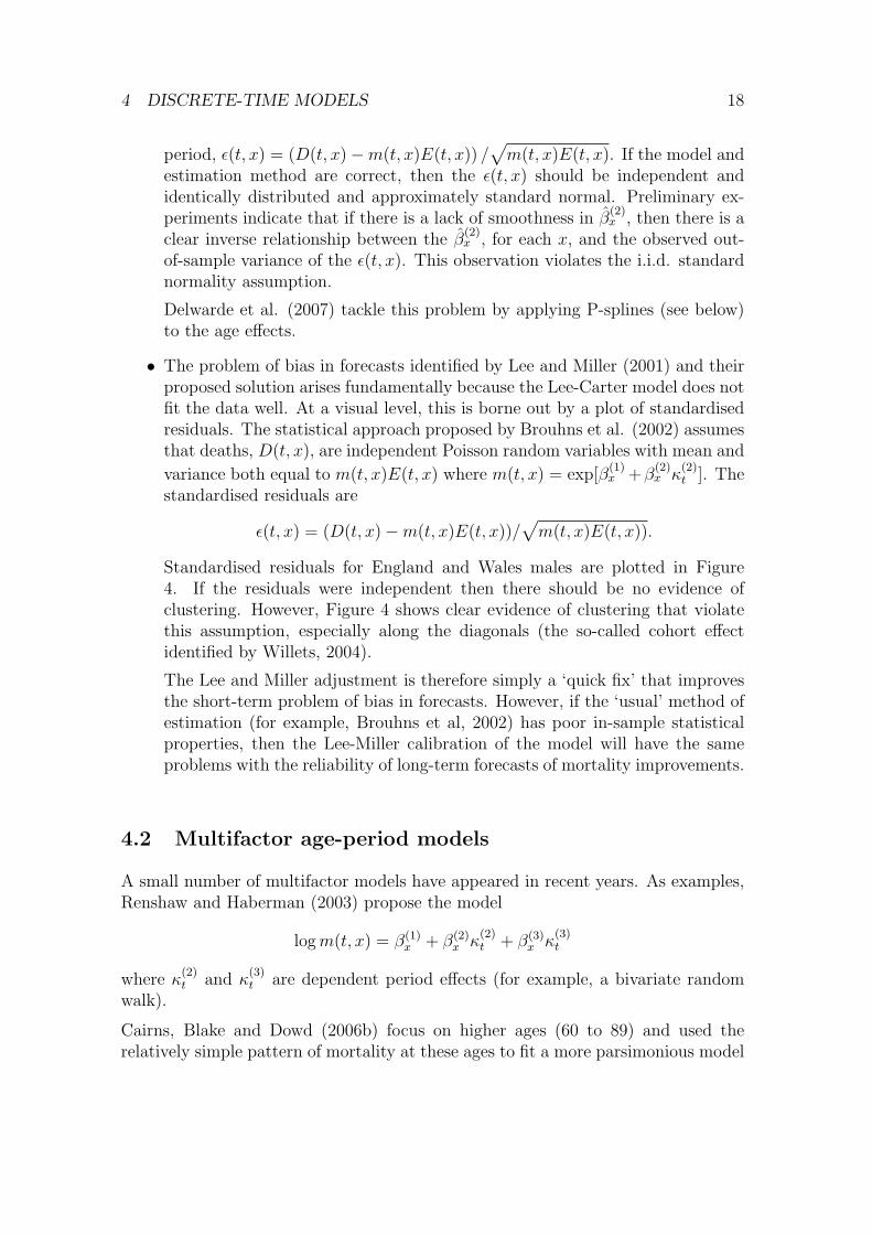
Parameter estimates for this model for England and Wales males aged 60 to 89 areplotted in Figure 6. From this we can make the following observations:

• κ(1)t (which can be interpreted as the ‘level’ of mortality) has a downwards

trend, reflecting generally improving mortality rates over time.

• κ(2)t (the ‘slope’ coefficient) has a gradual upwards drift, reflecting the fact

that, historically, mortality at high ages has improved at a slower rate than atyounger ages.

• κ(3)t (the ‘curvature’ coefficient) is more erratic, but has increased between

1961 and 2004.

• γ(4)c , where c = t − x, fluctuates around zero with no systematic trend or

curvature.


For forecasting, we need to develop models for the future dynamics of the periodand cohort effects. A simple starting point is to use a 3-dimensional random walkmodel for κ

(1)t , κ

(2)t , and κ

(3)t (see, for example, Cairns et al, 2008). However, there

are potential dangers with this approach:

• Based on the information in Figure 6, the random walk model for κ(3)t is

likely to have a positive drift. As κ(3)t becomes more and more positive, the

curvature of logit q(t, x) would become more and more positive over time. Wetherefore need to question whether or not this increasing curvature could resultin biologically unreasonable mortality curves. Possible compromises are to fita random-walk model to κ

(3)t with zero drift, or to fit a process (e.g. AR(1))

that is mean reverting to some possibly non-zero level.

• The upward trend for κ(2)t is more pronounced than it is for κ

(3)t and similar

comments might apply if we were to fit a random walk model with positivedrift to κ

(2)t . Specifically, this would result in mortality curves at high ages

becoming gradually steeper over time, and we have to question whether or notthis is biologically plausible. So, again, a model with no drift or even meanreversion might be biologically more reasonable, despite the observed strongupward trend in κ

(3)t .

Although not obvious, it is by design (see the Appendix) that the cohort effect, γ(4)c ,

looks like a process that is mean reverting to zero. This means that it is naturalto fit an AR(1) or some other mean-reverting process to γ

(4)c . Making this a mean-

reverting process, prevents γ(4)t−x from being decomposed into age-period effects. In

some other models that have been considered (see Cairns et al., 2007), the cohorteffect appears to have a linear drift. But linear drift in the cohort effect can oftenbe transformed into additional age-period effects. This raises the possibility thatsuch models could be improved by incorporating additional age-period effects andperhaps simplifying the form of the cohort effect.

4.5 P-splines

An approach that has become popular in the UK is the use of penalised splines(P-splines) (Currie et al., 2004, CMI, 2006). A typical model takes the form

log m(t, x) =∑i,j

θijBij(t, x)

where the Bij(t, x) are pre-specified basis functions with regularly-spaced knots, andthe θij are parameters to be estimated. It is well known that the use of splines canlead to functions that are over-fitted, resulting in fitted mortality surfaces that are


1960 1970 1980 1990 2000

−3.

4−

3.0

−2.

6−

2.2

Kappa_1(t)

Year, t

1960 1970 1980 1990 2000

0.08

0.09

0.10

0.11

Kappa_2(t)

Year, t

1960 1970 1980 1990 2000−0.

0015

−0.

0010

−0.

0005

0.00

000.

0005

Kappa_3(t)

Year, t

1880 1900 1920 1940

−0.

050.

000.

050.

10

Gamma_4(t)

Year, t

Figure 6: England & Wales data: Parameter estimates for the three-factor Cairns-Blake-Dowd cohort model. Crosses in the bottom right plot correspond to excludedcohorts.


unreasonably lumpy. P-splines avoid this problem by penalising roughness in theθij (for example, using linear or quadratic penalties). This approach has proven tobe very effective at producing globally a good fit (CMI, 2006). However, excessivesmoothing in the period dimension can lead to systematic over- or under-estimationof mortality rates, as the model fails to capture what may be genuine environmentalfluctations from one year to the next that affect all ages in the same direction (Cairnset al., 2007). To avoid this problem, Currie (personal communication) is developinga variant that adds annual shocks to an underlying mortality surface that is smoothin both the age and period dimensions.

4.6 Philosophical issues

The last remarks draw attention to some philosophical differences between ap-proaches. Specifically, to what extent should the fitted mortality surface be smooth?

A recent extension of the P-splines approach developed by Kirkby and Currie (2007)suggests that underlying mortality rates (the signal) are smooth, but we observe asignal plus noise where the noise is a systematic effect across all ages that is specificto each calendar year and which reflects ‘local’ conditions. The other models thathave been discussed so far assume that we observe the signal with no systematic noise(the independent Poisson assumption about mortality rates). Amongst these othermodels, there are varying assumptions about smoothness in individual dimensions.The Lee-Carter and Renshaw-Haberman models do not assume smoothness in theage or cohort effects. In contrast, the Cairns-Blake-Dowd cohort model outlined inSection 4.4 assumes smoothness in the age effect, but not in the cohort effect.

With the limited amount of data at our disposal, it remains a matter for debate asto how much smoothness should be assumed.

4.7 Discrete-time market models

In the field of interest-rate modelling, market models are ones that model the ratesthat are directly traded in the market such as LIBOR rates or swap rates. Thereare a number of equivalent approaches that can be taken in the stochastic modellingof mortality rates. In this section, we will consider a hypothetical market in zero-coupon longevity bonds with a full range of ages and terms to maturity. The priceat time t, as remarked earlier, of the (T, x)-bond that pays C(T )S(T, x) at time Tis denoted by BCS(t, T, x).

For the market to be arbitrage free, we require the existence of a risk-neutral mea-sure, Q, under which the discounted asset price, BCS(t, T, x)/C(t) = EQ[S(T, x)|Mt],is a martingale. Using the terminology of forward survival probabilities (equations1 and 3), we have pQ(t, T0, T1, x) = BCS(t, T1, x)/BCS(t, T0, x). The martingale

5 CONTINUOUS-TIME MODELS 26

property of discounted asset prices means that

pQ(t, t, T, x) = EQ[pQ(t + 1, t, T, x)|Mt] (5)

for all t < T and for all x. (Recall that (equation 3) pQ(t + 1, t, T, x) ={S(t +

1, x)/S(t, x)}pQ(t + 1, t + 1, T, x).)

Market models simultaneously model the prices of all of the type-B (T, x)-longevitybonds. This approach was first adopted in the Olivier-Smith model (see Olivier andJeffery, 2004, and Smith, 2005) which assumes for all t ≤ T and for all x:

pQ(t + 1, T, T + 1, x) = pQ(t, T, T + 1, x)b(t+1,T,T+1,x)G(t+1)

where G(1), G(2), . . . is a sequence of independent and identically distributed Gammarandom variables with both shape and scaling parameters equal to some constant α.The function b(t + 1, T, T, x) is measurable at time t and is a normalising constantthat ensures that equation (5) is satisfied. This suffers the drawback that it is aone-factor model that results in (a) lack of control over variances of mortality ratesat individual ages and (b) perfect correlation between mortality improvements atdifferent ages.

The use of a Gamma random variable has two advantages over possible alternatives.It makes the calculations analytically tractible, and it ensures that risk-neutral for-ward survival probabilities remain between 0 and 1.

Cairns (2007) proposes a generalisation of the Olivier-Smith model that moves awayfrom dependence on a single source of risk and allows for full control over the vari-ances and correlations:

pQ(t + 1, t, T, x) = pQ(t, t, T, x)eg(t+1,T,x)G(t+1,T,x). (6)

In this model, the g(t + 1, T, x) are again normalising constants that ensure themartingale property is satisfied. The G(t + 1, T, x) are dependent Gamma randomvariables that are specific to each maturity date T and to each age x. Cairns (2007)leaves as an open problem how to generate the Gamma random variables and pro-vides a detailed discussion of why this is, potentially, a difficult challenge. However,if this problem can be overcome then the generalised model has considerable poten-tial.

5 Continuous-time models

Even though data are typically reported in aggregate and at discrete intervals (e.g.annually), it is natural to consider the development of mortality rates in continuoustime. Cairns, Blake and Dowd (2006a) identify four frameworks that can be usedin the development of continuous-time models:3

3The discrete-time models described in Section 4 can all be described as short-rate models, withthe exception of the market model is Section 4.7.


• short-rate models – models for the one-dimensional (in x) instantaneous forceof mortality µ(t, x);

• forward-rate models – models for the two-dimensional (in age x, and maturityT ) forward mortality surface, µ(t, T, x + T ) (equation 4);

• market models – models for forward survival probabilities or annuity prices;

• positive mortality models – models for the spot survival probabilities.

No models have been proposed so far under the positive mortality framework, sothis approach is not discussed further in this article.

5.1 Philosophy: diffusions or jumps

Before we progress to consider specific continuous-time frameworks and models, wewill digress briefly to consider what underlying stochastic processes to use. Mostmodelling work to date has focused on the use of diffusion processes: that is, mor-tality dynamics are driven by one or more underlying Brownian motions. However,there is the possibility that these Brownian motions might be replaced or supple-mented by the use of jump processes. Jumps in the mortality process might occurfor a variety of reasons: sudden changes in environmental conditions, or radicalmedical advances.

If they are included, jumps might have one of two effects. In the simplest case,they have a direct impact on the instantaneous force of mortality, µ(t, x). Examplesof this might include a sudden pandemic or war. However, it is plausible that thesudden annoucement at time t of, for example, a cure for cancer might not havesuch an immediate impact. Instead, the cure might take time to become widelyused and implemented effectively. This would imply that there is no jump in thespot instantaneous force of mortality. However, the discovery might cause a jumpin the improvement rate of µ(t, x). As a consequence, forward mortality rates wouldalso jump, with larger jumps the further into the future.

Models with jumps are in their infancy (see, for example, Hainaut and Devolder,2007, and Chen and Cox, 2007), but their use will require just as much care in termsof model evaluation (see Section 3.1). Thus, for example, the inclusion of jumps willneed to be motivated by sound biological reasoning, rather than their inclusion forthe sake of mathematical generalisation.

As a final remark, the discrete nature of mortality data inevitably makes the useof jump models versus diffusion models a matter of speculation: if we only observethe process annually then we cannot observe jumps directly: instead, we can onlyobserve the compounded effect of jumps. Again, therefore, this places a degree of


responsibility on modellers to provide a good biological justification for the inclusionof jumps.

5.2 Short-rate models

Continuous-time short-rate models have, to date, proved the most fruitful source ofnew models. Models are of the type:

dµ(t, x) = a(t, x)dt + b(t, x)′dW (t)

where a(t, x) is the drift, b(t, x) is an n × 1 vector of volatilities, and W (t) is astandard n-dimensional Brownian motion under the risk-neutral measure, Q. Risk-neutral spot survival probabilities (assuming an arbitrage-free market) are then givenby (see, for example, Milevsky and Promislow, 2001, or Dahl, 2004)

pQ(t, T, x) = E

[exp

(−

∫ T

t

µ(u, x + u)du

) ∣∣∣∣ Mt

].

The drift and volatility processes will almost certainly depend on the current termstructure of mortality to ensure that the mortality curve remains positive and retainsa biologically reasonable shape. (For further discussion, see Cairns et al. (2006a).)

If a(t, y) and b(t, y) satisfy cetain conditions (see Dahl, 2004), we have a closed-formexpression for the spot survival probabilities:

pQ(t, T, x) = exp [A0(t, T, x)− A1(t, T, x)µ(t, x + t)] . (7)

Models where the logarithm of the spot survival probability is a linear function of thecurrent force of mortality are referred to as affine models, and have become the mostpopular of the stochastic mortality models for their analytical tractability (Dahl,2004, Biffis, 2005, Biffis and Millossovich, 2006, Dahl and Møller, 2006, Schrager,2006). Non-affine models have been developed by Milevsky and Promislow (2001)and Biffis et al. (2006).

Dahl and Møller (2006) develop a one-factor mortality model and use the concept ofmortality improvement factors to relate the future force of mortality to the currentmortality term structure:

µ(t, x + t) = µ(0, x + t)ξ(t, x + t)

where ξ(t, x + t) is the improvement factor with dynamics

dξ(t, y) = (γ(t, y)− δ(t, y)ξ(t, y)) dt + σ(t, y)√

ξ(t, y)dW (t).

Thus, ξ(t, y) takes the form of a time-inhomogeneous Cox, Ingersoll and Ross (1985)model (CIR). This model satisfies the criterion for an affine mortality term structure


and so spot survival probabilities take the form (7). The deterministic functionsγ(t, y) and δ(t, y) allow for considerable flexibility in terms of the rate at whichmortality is predicted to improve over time. It does require mean reversion (that is,δ(t, y) > 0; see Section 3.3), but it is argued that this mean reversion can be relativelyweak and, therefore, is a minor disadvantage when compared with the advantagesof tractability. Dahl and Møller (2006) give examples for γ(t, y), δ(t, y) and σ(t, y)that take particular parametric forms that are then calibrated approximately toDanish mortality data. A more general two-factor model is proposed by Biffis andMillossovich (2006).

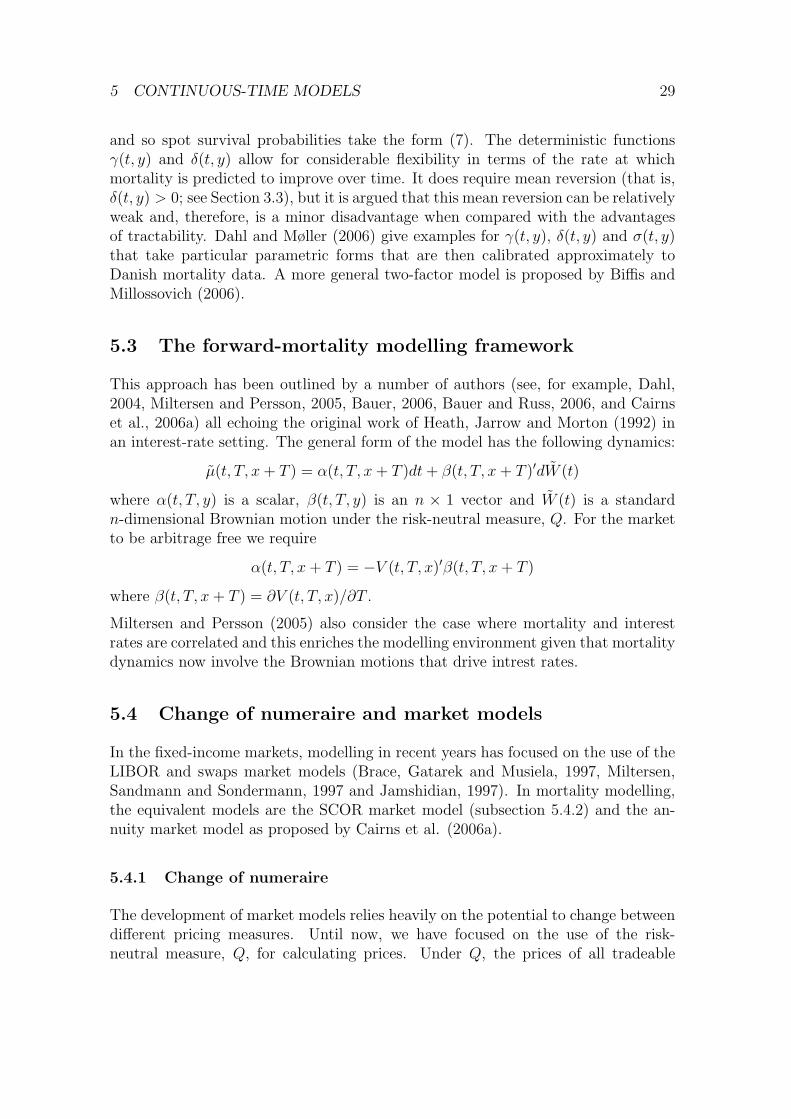
5.3 The forward-mortality modelling framework

This approach has been outlined by a number of authors (see, for example, Dahl,2004, Miltersen and Persson, 2005, Bauer, 2006, Bauer and Russ, 2006, and Cairnset al., 2006a) all echoing the original work of Heath, Jarrow and Morton (1992) inan interest-rate setting. The general form of the model has the following dynamics:

µ(t, T, x + T ) = α(t, T, x + T )dt + β(t, T, x + T )′dW (t)

where α(t, T, y) is a scalar, β(t, T, y) is an n × 1 vector and W (t) is a standardn-dimensional Brownian motion under the risk-neutral measure, Q. For the marketto be arbitrage free we require

α(t, T, x + T ) = −V (t, T, x)′β(t, T, x + T )

where β(t, T, x + T ) = ∂V (t, T, x)/∂T .

Miltersen and Persson (2005) also consider the case where mortality and interestrates are correlated and this enriches the modelling environment given that mortalitydynamics now involve the Brownian motions that drive intrest rates.

5.4 Change of numeraire and market models

In the fixed-income markets, modelling in recent years has focused on the use of theLIBOR and swaps market models (Brace, Gatarek and Musiela, 1997, Miltersen,Sandmann and Sondermann, 1997 and Jamshidian, 1997). In mortality modelling,the equivalent models are the SCOR market model (subsection 5.4.2) and the an-nuity market model as proposed by Cairns et al. (2006a).

5.4.1 Change of numeraire

The development of market models relies heavily on the potential to change betweendifferent pricing measures. Until now, we have focused on the use of the risk-neutral measure, Q, for calculating prices. Under Q, the prices of all tradeable


assets discounted by the cash account, C(t), are martingales. Recall, therefore, theprice of the type-B (T, x)-longevity bond (equation 2). The discounted asset priceis

BCS(t, T, x) =BCS(t, T, x)

C(t)= EQ[S(T, x)|Mt].

In a continuous-time diffusion setting, the dynamics of this discounted price processcan be written as

dBCS(t, T, x) = BCS(t, T, x)V (t, T, x)′dW (t)

where V (t, T, x) is a previsible n× 1 process and W (t) is a standard n-dimensionalBrownian motion under Q. In these expressions, we have used the cash accountC(t) as the numeraire. But we can use the prices of other tradeable assets (providedthese prices remain positive) as alternative numeraires. For example, if we takeBCS(t, τ, x) as the numeraire, and define Z(t, T, x) = BCS(t, T, x)/BCS(t, τ, x), then

dZ(t, T, x) = Z(t, T, x)(V (t, T, x)− V (t, τ, x)

)′(dW (t)− V (t, τ, x)dt

).

We now define dW τ,x(t) = dW (t)− V (t, τ, x)dt and note that this depends only onthe volatility of the numeraire and not on any characteristics of the (T, x)-longevitybond. Provided that V (t, τ, x) satisfies the Novikov condition (see, for example,Karatzas and Shreve, 1998), there exists a measure Pτ,x equivalent to Q underwhich the resulting process, W τ,x(t), is a standard Brownian motion. Under Pτ,x

the Z(t, T, x) are martingales for all t < T and t < τ : that is

dZ(t, T, x) = Z(t, T, x)(V (t, T, x)− V (t, τ, x)

)′dW τ,x(t).

Why is a change of numeraire relevant? First, in interest-rate modelling, it wasdiscovered, that the pricing of interest-rate derivatives could sometimes be simpli-fied by making a change of measure (see, for example, Cairns, 2004). Second, theLIBOR and swap market models both rely on a change of measure as a fundamentalstep in defining the model dynamics. Third, if we make certain assumptions aboutthe volatility, then the use of models that exploit a change of numeraire makes itstraightforward to value key option contracts.

5.4.2 The SCOR market model

The Survivor Credit Offered Rate (SCOR; first proposed by Cairns, Blake and Dowd,2006a) is similar to the bonus in a traditional with-profits insurance contract wherethe bonus is linked solely to the historical development of mortality rates. A minordifference, though, is that the SCOR represents a bonus rate that is set one year inadvance of its payment. By analogy with forward LIBOR rates, the forward SCORs(t, T, T + 1, x) can be linked to a financial and mortality-linked derivative with thefollowing terms (for variants on the contract below, see Cairns et al., 2006a):


• At time t, no money exchanges hands, and the value of the derivative is zero.

• At time T , the contract-holder will pay a fixed amount, K, to the counterparty,to be invested in the risk-free cash account, C(u).

• At time T + 1, the contract-holder will receive

K × C(T + 1)/C(T )× (1 + s(t, T, T + 1, x))

)× (1− q(T, x + T )

)

where q(T, x + T ) is the realised mortality rate between T and T + 1 of indi-viduals aged x + T at time T : that is, 1− q(T, x + T ) = S(T + 1, x)/S(T, x).

The rate that ensures that this contract has zero value at time t is (see Cairns etal., 2006a)

s(t, T, T + 1, x) =pQ(t, T, x)− pQ(t, T + 1, x)

pQ(t, T + 1, x)

=BCS(t, T, x)−BCS(t, T + 1, x)

BCS(t, T + 1, x). (8)

Variants of this contract can link the initial payment to financial markets up to Tor, for example, to the survivor index iteslf (Cairns et al, 2006a).

The forward SCOR (equation 8) is therefore the ratio of the value of a portfolio(long in the (T, x)-longevity bond and short in the (T +1, x)-longevity bond) to theprice of the (T +1, x)-longevity bond. It follows that the forward SCOR, s(t, T, T +1, x) must be a martingale under the (T + 1, x)-forward measure PT+1,x. We can,therefore, mimic the LIBOR market model by postulating that if the volatility ofs(t, T, T +1, x) is deterministic, then s(T, T, T +1, x) will be log-normal under PT+1,x

(an admissible distribution, since the forward SCOR can take any value between 0and ∞). This property then allows straightforward construction of option-typederivatives on s(T, T, T + 1, x) with Black-Scholes-type pricing formulae (Cairns etal, 2006a).

5.4.3 Individual insurance

In an insurance context, the contract-holder is a policyholder who is aged x + t attime t, with survival function Ix(u) = 1 if the policyholder is still alive at time uand 0 otherwise. The cashflows to the policyholder are then replaced by −KI(T )

at time T and K C(T+1)C(T )

(1+ s(t, T, T +1, x))I(T +1). K might be linked to financialand other events up to time T . The SCOR then represents a bonus rate payableto survivors, while assets belonging to policyholders who die revert to the insurer.A traditional annuity contract is, indirectly, an example of such an arrangement.Provided the market price of non-systematic mortality risk is zero, this variant ofthe SCOR is priced in the same way as above (see Cairns et al., 2006a).

6 THE MANAGEMENT OF MORTALITY RISK 32

5.5 Forward-rate and market models: advantages and dis-advantages

In certain cases, forward-rate and market models offer the possibility of analyticaltractability. But the key advantage of forward-rate and market models is that, atany future date t, they automatically provide as output a two-dimensional forwardmortality table (pQ(t, T, x) for all T and x). This means that it is easy to computethe payoff on a contract that is linked to the 2-dimensional mortality table that is inuse at time t (for example, a guaranteed annuity contract). With some exceptions(e.g. Dahl, 2004), it is not straightforward to compute such a 2-dimensional tableusing short-rate models. In some cases (see, for example, Dowd et al, 2007) thisproblem can be mitigated through the use of good analytical approximations forkey outputs as functions of the finite number of underlying state variables.

But forward-rate and market models have their limitations. First, they require asinput at time 0, a complete 2-dimensional set of market spot survival probabilities.At the present time, such market-determined variables do not exist. (Market annuityprices do offer a partial solution, but these can be heavily distorted by expenseloadings.) Instead, it will be necessary to use tables of projected survival ratesusing other models. Second, the longest maturity date that is input at time 0 placesa limit on the length of each sample path: that is, we can only follow the paths ofSCOR rates, s(t, T, T +1, x), that are input at time 0, and each SCOR rate ‘expires’at its respective payment date T + 1.

6 The management of mortality risk

Recent years have seen a growing realisation that mortality risk can be significantfor financial institutions such as life assurers and pension plans (see, for example,O’Brien, 1999). Depending upon how such institutions have invested their assets,mortality risk might not be the largest risk they face, but it is often significantand one that cannot be ignored. Instead, modern risk-management practice re-quires companies to manage mortality risk as effectively as possible as part of awider framework of enterprise risk management rather than to accept its presenceas inevitable.

A range of possible responses to longevity risk is possible, some depending on thetype of institution (see, for example, Blake et al., 2006).

• Assurers can retain mortality risk as a legitimate business risk. This assumesthat the company is able to achieve an adequate expected rate of return relativeto the level of risk being carried.

• Assurers can diversify their mortality risk across product ranges, regions and


socio-economic groups. An example of this includes natural hedging (see, forexample, Cox and Lin, 2004) where gains on the life book will balance losseson the annuity book.

• They can enter into a variety of forms of full or partial reinsurance, in orderto hedge downside mortality risk.

• Pension plans can arrange a full or partial buyout of their liabilities by a spe-cialist insurer (e.g. Paternoster in the UK). (Small pension plans in the UKare exposed to considerable non-systematic mortality risk and often, there-fore, purchase annuities from a life office for employees at the time of theirretirement, thereby removing the tail mortality risk.)

• For future annuity and pension provision, non-profit contracts could be re-placed by participating annuities. Such annuities might share mortality profitsor losses by adjusting the amounts of pensions in payment or by linking thedate of retirement to current life expectancy.

• Assurers can securitise a line of business (see, for example, Cowley and Cum-mins, 2005).

• Mortality risk can be managed through the use of mortality-linked securitiesand derivatives. This approach differs from the securitisation of a line ofbusiness as the financial securities concerned have cashflows that are purelylinked to the future value of a mortality index, rather than being a complexpackage of business risks.

We will focus here on the last of these possibilities, mortality-linked securities andderivatives, which have recently been made available by the establishment of a newcapital market called the ‘life market’. Loeys et al. (2007, p.6) show that for a newcapital market to become established and to flourish: “it (1) must provide effectiveexposure, or hedging, to a state of the world that is (2) economically important andthat (3) cannot be hedged through existing market instruments, and (4) it must usea homogeneous and transparent contract to permit exchange between agents.” Theyargue that a market trading mortality risk meets these criteria and that a successfulmarket should emerge in due course.

We will now describe briefly the different types of security that could be used.

6.1 Mortality catastrophe bonds

Although this paper is primarily concerned with mortality risk, it is, nevertheless,instructive to discuss short-dated mortality catastrophe bonds, since there have beena number of successful issues of this type of bond. They are market-traded securities


whose payments are linked to a mortality index. They are similar to catastrophebonds.

The first such bond issued was the Swiss Re bond (known as Vita I) which came tomarket in December 2003. This was designed to securitise Swiss Re’s own exposureto mortality risk. Vita I was a 3-year bond (maturing on 1 January 2007) whichallowed the issuer to reduce exposure to certain catastrophic mortality events: asevere outbreak of influenza, a major terrorist attack (using weapons of mass de-struction) or a natural catastrophe. The mortality index was weighted by age, sexand nationality. The $400m principal was at risk if, during any single calendar year,the combined mortality index exceeded 130% of the baseline 2002 level, and wouldbe exhausted if the index exceeded 150%. In return for having their principal at risk,investors received quarterly coupons of 3-month US LIBOR plus 135 basis points.

The success of the bond led to additional bonds being issued on much less favourableterms to investors: for example, Vita II by Swiss Re in 2005 ($362m), Vita III bySwiss Re in 2007 ($705m), Tartan by Scottish Re in 2006 ($155m) and OSIRIS byAXA in 2006 ($442m).

6.2 Mortality (or survivor) swaps

The key derivative of interest is the mortality (or survivor) swap (e.g., Dowd etal (2006), see also Lin and Cox (2005)). Counterparties swap fixed series of pay-ments in return for series of payments linked to the number of survivors in a givencohort. One example would be a swap based on 65-year old males from Englandand Wales. As another example, a UK annuity provider could swap cashflows basedon a UK mortality index for cashflows based on a US mortality index from a USannuity provider counterparty: this would enable both counterparties to diversifytheir longevity risks internationally.

The world’s first publicly announced mortality swap took place in April 2007 be-tween Swiss Re and Friends’ Provident, a UK life assurer. It was a pure longevityrisk transfer and was not tied to another financial instrument or transaction. Theswap was based on Friends’ Provident’s £1.7bn book of 78,000 of pension annuitycontracts written between July 2001 and December 2006. Friends’ Provident re-tains administration of policies. Swiss Re makes payments and assumes longevityrisk in exchange for an undisclosed premium. However, it is important to note thatthis particular swap was legally constituted as an insurance contract and was not acapital market instrument.

In a further development in December 2007, Goldman Sachs launched a monthlyindex called QxX.LS (www.qxx-index.com) in combination with standardised 5 and10-year mortality swaps. The index is based on a pool of 46,290 anonymised livesover the age of 65 from a database of life-policy sellers (the so-called life-settlements


market) assessed by the medical underwriter AVS.

In a thorough and groundbreaking paper, Dahl et al. (2008) consider a situationwhere a mortality (or survivor) swap is used to hedge dynamically the mortality riskin a life book. An important contribution in Dahl et al.’s work is the acknowledge-ment that the reference population underlying the swap might be different from thatin the portfolio being hedged, and they carry out a detailed numerical example toillustrate the impact of the resulting basis risk. The tractability offered by the affinemodel they use allows a more straightforward development of hedging strategies formitigating mortality risk (one of our criteria for a good model: see subsection 3.1).In the case of Dahl et al.’s (2008) work, the analytical tractability of their affinemortality model makes it possible to implement and evaluate the effectiveness of adynamic hedging strategy. This recalls our earlier model evaluation criterion that itshould be straightforward to implement a model either analytically or using efficientnumerical algorithms.

6.3 Longevity (or survivor) bonds

The world’s first attempt to issue a longevity (or survivor) bond was in November2004. The European Investment Bank (EIB) offered to issue a 25-year longevitybond with an issue price of £540m and an initial coupon of £50m. The referencesurvivor index, S(t), was based on 65-year-old males from the national populationof England and Wales as produced by the UK Government Actuary’s Department(GAD). The structurer/manager was BNP Paribas which assumed the longevity risk,but reinsured it through PartnerRe, based in Bermuda. The structure of the bond(see Blake et al., 2006, Figure 4) involves both a mortality swap and an interest-rate swap. The target group of investors was UK pension funds, but, for reasonsdiscussed in Blake et al. (2006), the bond did not attract sufficient investor interestand was later withdrawn.

6.4 Longevity-linked securities

A perceived problem with the EIB longevity bond was that the reference index mightnot be sufficiently highly correlated with a hedger’s own mortality experience (as aresult of basis risk). An alternative instrument, that we will refer to as a longevity-linked security (LLS), deals, at least partly, with this problem. The concept isinspired by the design of mortgage-backed securities. The LLS is built around aspecial purpose vehicle (SPV). Individual hedgers on one side of the contract (forexample, pension plans) arrange mortality swaps with the SPV using their ownmortality experience at rates that are negotiated with the SPV manager. Theswapped cashflows are then aggregated and passed on to the market. Bondholdersgain if mortality is heavier than anticipated.


It might be felt that the aggregate cashflows themselves lack transparency (this didnot seem to be a problem with mortgage-backed securities until the emergence of thecredit crunch in 2007) in which case the SPV might link cashflows to an acceptedreference index. The difference between this and the aggregated swap cashflows isa basis risk that is borne by the SPV manager.

This type of arrangement is illustrated in Figure 7. In this example, there are threehedgers, A, B, and C. Hedger A wishes to swap the risky longevity-linked cashflowsLA(t) for a series of pre-determined cashflows. The agreement with the SPV manageris to swap floating LA(t) for fixed LA(t) for t = 1, . . . , T , with the fixed leg set ata level that results in the swap initially having zero value at time 0. Similarly,hedger B swaps floating LB(t) for fixed LB(t), and hedger C floating LC(t) for fixedLC(t). The SPV itself invests in AAA-rated, fixed-interest securities of appropriateduration or uses floating rate notes plus an interest-rate swap. The LLS bondholderspay an initial premium that is used to buy the fixed-interest securities and to payan initial commission to the manager. The bondholders in return receive couponsand, possibly, a final repayment of principal that is linked either to the hedgers’floating cashflows or to a reference index that matches as closely as possible thecombined cashflows. In the latter case, any differences accrue to the SPV manager.The bondholders will not normally be hedgers themselves, so they will expect a fairpremium over market fixed-interest rates in return for assuming the mortality risk.


SPV

Bond Holders

Hedger A Hedger B Hedger C

Manager

6

?

MortalitySwap A

LA(t) LA(t)

6

?

MortalitySwap B

LB(t) LB(t)

6

?

MortalitySwap C

LC(t) LC(t)

-

-¾

Commission

Basis risks

6

?

InitialPremium

Longevity-linkedCoupons & Principal

Figure 7: Cashflows under a longevity-linked security (LLS). Bondholders mightreceive cashflows linked to a reference index rather than LA(t), LB(t) and LC(t), inwhich case residual basis risk must be borne by the SPV manager.


Counterparty A(fixed rate payer)

Counterparty B(fixed rate receiver)

-

¾

Notional × 100 ×fixed mortality rate

Notional × 100 ×realised mortality rate

Figure 8: A q-forward arranged at time t exchanges fixed mortality, qF (t, T, y), forrealised mortality, q(T, y), at maturity, T + 1, of the contract. (Source: Coughlanet al. (2007, Figure 1))

6.5 Mortality (or q-) forwards

In July 2007, JPMorgan announced the launch of a mortality forward contract withthe name ‘q-forward’ (Coughlan et al., 2007). It is a forward contract linked to afuture mortality rate, taking its name from the standard actuarial notation, ‘q’, fora mortality rate. The contract involves the exchange, at time T + 1, of a realisedmortality rate, q(T, x), relating to a specified population on the maturity date of thecontract, in return for a fixed mortality rate agreed at the beginning of the contract(Figure 8).

A series of q-forward contracts, with different ages, can be combined to hedge,approximately, a mortality swap. As an example, suppose the contract involvesswapping at time t a fixed cashflow, S(t), for the realised survivor index, S(t, x).The fixed leg can be hedged using zero-coupon fixed-income bonds. The floatingleg can be hedged approximately as follows. First, note that we can approximatethe survivor index by expanding the cashflow in terms of the fixed legs of a set ofq-forwards and their ultimate net payoffs:

S(t, x) = (1− q(0, x))× (1− q(1, x + 1))× . . .× (1− q(t− 1, x + t− 1))

=t−1∏i=0

(1− qF (0, i, x + i)−∆(i, x + i)

)

≈t−1∏i=0

(1− qF (0, i, x + i)

)

−t−1∑i=0

∆(i, x + i)t−1∏

j=0,j 6=i

(1− qF (0, j, x + j)

)

where ∆(i, x + i) = q(i, x + i)− qF (0, i, x + i)

and qF (0, i, x + i) = q-forward mortality rate (the fixed rate).

Here, ∆(i, x + i) is the net payoff on the q-forward per unit at time i + 1.


It follows that an approximate hedge (assuming interest rates are constant and equalto r per annum) for S(t, x) can be achieved by holding:

• −(1 + r)−(t−1)∏t−1

j=0,j 6=0(1− qF (0, j, x + j)) units of the 1-year q-forward;

• −(1 + r)−(t−2)∏t−1

j=0,j 6=1(1− qF (0, j, x + j)) units of the 2-year q-forward;

• ...

• −∏t−1j=0,j 6=(t−1)(1− qF (0, j, x + j)) units of the t-year q-forward.

In calculating these hedge quantities, we take account of the fact that, for example,the payoff at time 1 on the 1-year q-forward will be rolled up to time t at the risk-freerate of interest. Hence, the required payoff at time t needs to be multiplied by thediscount factor (1+r)−(t−1). In a stochastic interest environment, a quanto derivativewould be required. A quanto derivative is one that delivers a number of units, N , ofa specified asset, where N is derived from a reference index that is different from theasset being delivered. In this context, N equals −∆(i, x+ i)

∏t−1j=0,j 6=i(1−qF (0, j, x+

j)), and we deliver, at time i + 1, N units of the fixed-interest zero-coupon bondmaturing at time t, price P (i + 1, t) at time i + 1 per unit.

The discussion above covers the ‘pure’ version of the q-forward contract. However,some practical issues come into play. First, the hedging arguments here would needmodification if, as is likely, q-forwards are subject to annual margin calls that resultin the contracts being marked-to-market. Second, in order to keep the number ofcontracts to a manageable level, individual contracts use the average (or ‘bucketed’)mortality across 10 ages rather than single ages. This averaging has positive andnegative effects. On the one hand, the averaging reduces the basis risk that arisesfrom the non-systematic mortality risk that is present in crude mortality rates, evenat the population level. On the other hand, it introduces some basis risk dependingon the specific age-structure of the population being hedged.

6.6 Forward SCOR

For completeness, we will recall subsection 5.4.2 where we introduced the forwardSCOR contract. This contract is closely linked to the q-forward contract since thepayoff structure involves both the SCOR rate and the mortality rate underlying theq-forward. The two are related, additionally, by the relationships

EQ[q(T, x)|MT ] =s(T, T, T + 1, x− T )

1 + s(T, T, T + 1, x− T )

⇒ EQ[q(T, x)|Mt] = EQ

[s(T, T, T + 1, x− T )

1 + s(T, T, T + 1, x− T )

∣∣∣∣ Mt

]for t < T .

7 CONCLUSIONS 40

6.7 Mortality options, and longevity (or survivor) caps andfloors

Mortality options give payoffs that are non-linear functions of underlying variablesand are attractive to (a) hedgers who might wish to protect their downside exposure,but leave any upside potential, and (b) speculators who want to trade views onvolatility rather than views on the level of mortality (or related, e.g. annuity) rates.

In the case of longevity (or survivor) caps and floors, the underlying is a survivorindex S(t, x). Suppose sc(t) is a cap rate for exercise date t, while sf (t) is thecorresponding floor rate. A caplet will pay max{S(t, x) − sc(t), 0} at time t, whilea floorlet will pay max{sf (t) − S(t, x), 0}. Series of caplets and floorlets then getpackaged into caps and floors.

7 Conclusions

There have been tremendous conceptual advances in both the modelling and man-agement of mortality risk in recent years. These advances are not unrelated. Agood stochastic mortality model is a virtual prerequisite to the successful introduc-tion of a capital market in mortality hedging instruments. Where we consider thedevelopment of other markets, such as that for interest-rate derivatives, we can notethat the early days were characterised by pricing-to-model, but once the markethad become sufficiently deep and liquid, the models could be dropped in favour ofpricing-to-market. The same is likely to happen in the life market. But the de-velopment of a good and reliable model requires time and considerable patience:an initial analysis might suggest that a model is satisfactory, but further forensicinvestigation might reveal some pitfalls that need corrective work. However, thisdevelopment time can repay itself handsomely through greater understanding of theunderlying process driving mortality rate dynamics.

There are still considerable challenges ahead. The existing models need furtherrefinement; the market in mortality-linked derivatives is still in its infancy; and westill need to develop further our understanding of how these contracts can be usedin the most effective way to manage mortality risk.

8 REFERENCES 41

8 References

Bauer, D. (2006) “An arbitrage-free family of longevity bonds”, Working paper,University of Ulm. See www.mortalityrisk.org

Bauer, D., and Russ, J. (2006) “Pricing longevity bonds using implied survivalprobabilities”, Working paper, University of Ulm. See www.mortalityrisk.org

Biffis, E. (2005) “Affine processes for dynamic mortality and actuarial valuations”,Insurance: Mathematics and Economics, 37: 443-468.

Biffis, E., Denuit, M., and Devolder, P. (2006) “Stochastic mortality under measurechanges”, Pensions Institute Discussion Paper PI-0512. (April 19, 2006 version)

Biffis, E., and Millossovich, P. (2006) “The fair value of guaranteed annuity options”,Scandinavian Actuarial Journal, 2006(1): 23-41.

Blake, D., and Burrows, W. (2001) “Survivor bonds: Helping to hedge mortalityrisk”, Journal of Risk and Insurance, 68: 339-348.

Blake, D., Cairns, A.J.G., and Dowd, K. (2006) “Living with mortality: Longevitybonds and other mortality-linked securities.” (with discussion) British ActuarialJournal, 12: 153-228.

Booth, H., Maindonald, J., and Smith, L. (2002) “Applying Lee-Carter underconditions of variable mortality decline”, Population Studies, 56: 325-336.

Brace, A., Gatarek, D., and Musiela, M. (1997) “The market model of interest-ratedynamics”, Mathematical Finance, 7: 127-155.

Brigo, D., and Mercurio, F. (2001) “Interest Rate Models: Theory and Practice”Springer, Berlin.

Brouhns, N., Denuit, M., and Vermunt J.K. (2002) “A Poisson log-bilinear regres-sion approach to the construction of projected life tables”, Insurance: Mathematicsand Economics, 31: 373-393.

Cairns, A.J.G. (2004) “Interest Rate Models: An Introduction”, Princeton Univer-sity Press, Princeton.

Cairns, A.J.G. (2007) “A multifactor generalisation of the Olivier-Smith model forstochastic mortality”, In Proceedings of the 1st IAA Life Colloquium, Stockholm,2007.

Cairns, A.J.G., Blake, D., and Dowd, K. (2006a) “Pricing death: Frameworks forthe valuation and securitization of mortality risk”, ASTIN Bulletin, 36: 79-120.

Cairns, A.J.G., Blake, D., and Dowd, K. (2006b) “A two-factor model for stochasticmortality with parameter uncertainty: Theory and calibration”, Journal of Riskand Insurance, 73: 687-718.

8 REFERENCES 42

Cairns, A.J.G., Blake, D., Dowd, K., Coughlan, G.D., Epstein, D., Ong, A., andBalevich, I.(2007) “A quantitative comparison of stochastic mortality models usingdata from England & Wales and the United States”, Working paper, Heriot-WattUniversity, and Pensions Institute Discussion Paper PI-0701.

Cairns, A.J.G., Blake, D., Dowd, K., Coughlan, G., Epstein, D., and Khallaf-Allah,M. (2008) “The plausibility of mortality density forecasts: an analysis of six stochas-tic mortality models”, Working paper, Heriot-Watt University, and Pensions Insti-tute Discussion Paper PI-0801.

Chen, H, and Cox, S.H. (2007) “Modeling mortality with jumps: Transitory effectsand pricing implication to mortality securitization”, Working paper, Georgia StateUniversity.

Continuous Mortality Investigation (CMI) (2006) “Stochastic projection method-ologies: Further progress and P-Spline model features, example results and implica-tions”, Working paper 20.

Continuous Mortality Investigation (CMI) (2007) “Stochastic projection method-ologies: Lee-Carter model features, example results and implications”, Workingpaper 25.

Coughlan, G., Epstein, D., Sinha, A. and Honig, P. (2007) “q-forwards: Derivativesfor transferring longevity and mortality risks”, JPMorgan Pension Advisory Group,London, July.

Cox, J., Ingersoll, J., Ross, S. (1985) “A theory of the term-structure of interestrates”, Econometrica, 53: 385-408.

Cox, S.H., and Lin, Y. (2004) “Natural hedging of life and annuity mortality risks”In Proceedings of the 14th International AFIR Colloquium, Boston, pp483-507.

Currie, I.D., Durban, M. and Eilers, P.H.C. (2004) “Smoothing and forecastingmortality rates”, Statistical Modelling, 4: 279-298.

Czado, C., Delwarde, A., and Denuit, M. (2005) “Bayesian Poisson log-linear mor-tality projections” Insurance: Mathematics and Economics, 36: 260-284.

Dahl, M. (2004) “Stochastic mortality in life insurance: Market reserves and mortality-linked insurance contracts”, Insurance: Mathematics and Economics, 35:113-136.

Dahl, M., and Møller, T. (2006) “Valuation and hedging of life insurance risks withsystematic mortality risk”, Insurance: Mathematics and Economics, 39: 193-217.

Dahl, M., Melchior, M., and Møller, T. (2008) “On systematic mortality risk and riskminimisation with survivor swaps”, Scandinavian Actuarial Journal, 2008(1):xxx-yyy.

De Jong, P., and Tickle, L. (2006) “Extending the Lee-Carter model of mortalityprojection”, Mathematical Population Studies, 13:1-18.

8 REFERENCES 43

Delwarde, A., Denuit, M., and Eilers, P. (2007) “Smoothing the Lee-Carter andPoisson log-bilinear models for mortality forecasting: A penalised log-likelihoodapproach”, Statistical Modelling, 7: 29-48.

Dowd, K. Blake, D., Cairns, A.J.G., and Dawson, P. (2006) “Survivor swaps”,Journal of Risk and Insurance, 73-1-17.

Dowd, K., Blake, D., and Cairns, A.J.G. (2007) “Facing up to uncertain life ex-pectancy: The longevity fan charts”, Pensions Institute Discussion Paper PI-0703.

Dowd, K., Blake, D., Cairns, A.J.G., Coughlan, G.D., Epstein, D., and Khalaf-Allah, M.(2008a) “Evaluating the goodness of fit of stochastic mortality models”,Forthcoming, Pensions Institute Discussion Paper PI-0802.

Dowd, K., Blake, D., Cairns, A.J.G., Coughlan, G.D., Epstein, D., and Khalaf-Allah, M.(2008b) “Backtesting stochastic mortality models: An ex-post evaluationof multi-period-ahead density forecasts”, Forthcoming, Pensions Institute DiscussionPaper PI-0803.

Hainaut, D., and Devolder, P. (2007) “Mortality modelling with Levy processes”,Working paper, Universite Catholique de Louvain.

Heath, D., Jarrow, R., and Morton, A. (1992) “Bond pricing the the term structureof interest rates: A new methodology for contingent claims valuation”, Economet-rica, 60: 77-105.

Hull, J., White, A. (1990) “Pricing interest-rate derivative securities”, Review ofFinancial Studies, 3: 573-592.

Jacobsen, R., Keiding, N., and Lynge, E. (2002) “Long-term mortality trends behindlow life expectancy of Danish women”, J. Epidemiol. Community Health, 56: 205-208.

Jamshidian, F. (1997) “LIBOR and swap market models and measures”, Financeand Stochastics, 1: 293-330.

Kirkby, J. G. and Currie, I. D. (2007) “Smooth models of mortality with periodshocks”, In Proceedings of 22nd International Workshop on Statistical Modelling,Barcelona, 374-379.

Lee, R.D., and Carter, L.R. (1992) “Modeling and forecasting U.S. mortality”, Jour-nal of the American Statistical Association, 87: 659-675.

Lee, R., and Miller, T. (2001) “Evaluating the performance of the Lee-Carter modelfor forecasting mortality”, Demography, 38: 537-549.

Lin, Y., and Cox, S.H. (2005) “Securitization of mortality risks in life annuities”,Journal of Risk and Insurance, 72, 227-252.

Milevsky, M.A., and Promislow, S.D. (2001) “Mortality derivatives and the optionto annuitise”, Insurance: Mathematics and Economics, 29: 299-318.

8 REFERENCES 44

Miltersen, K.R., Sandmann, K., and Sondermann, D. (1997) “Closed-form solutionsfor term structure derivatives with log-normal interest rates”, Journal of Finance,52: 409-430.

Miltersen, K.R., and Persson, S.-A. (2005) “Is mortality dead? Stochastic forwardforce of mortality determined by no arbitrage” Working paper, University of Bergen.

O’Brien, C. (1999) “Actuaries and accountability”, Presidential Address to theManchester Actuarial Society, 1999.

Olivier, P., and Jeffery, T. (2004) “Stochastic mortality models”, Presentation tothe Society of Actuaries of Ireland: see www.actuaries.ie (Events and Papers).

Osmond, C. (1985) “Using age, period and cohort models to estimate future mor-tality rates”, International Journal of Epidemiology, 14: 124-129.

Renshaw, A.E., and Haberman, S. (2003) “Lee-Carter mortality forecasting withage-specific enhancement,” Insurance: Mathematics and Economics, 33: 255-272.

Renshaw, A.E., and Haberman, S. (2006) “A cohort-based extension to the Lee-Carter model for mortality reduction factors”, Insurance: Mathematics and Eco-nomics, 38: 556-570.

Richards, S.J., Kirkby, J.G., and Currie, I.D. (2006) “The importance of year of birthin two-dimensional mortality data”, (with discussion) British Actuarial Journal, 12:5-61.

Schrager, D.F. (2006) “Affine stochastic mortality”, Insurance: Mathematics andEconomics 38:81-97.

Smith, A.D. (2005) “Stochastic mortality modelling”, Workshop on the Interface be-tween Quantitative Finance and Insurance, International Centre for the Mathemati-cal Sciences, Edinburgh. See www.icms.org.uk/archive/meetings/2005/quantfinance/

Vasicek, O. (1977) “An equilibrium characterization of the term structure”, Journalof Financial Economics, 5: 177-188.

Willets, R.C. (2004) “The cohort effect: Insights and explanations” British ActuarialJournal, 10: 833-877.

Appendix: Identifiability constraints

For the model discussed in Section 4.4 there is an identifiability problem. Thismodel, as with others such as the Lee-Carter model requires the use of identifia-bility constraints to ensure that the estimation problem is well-specified. For thismodel we have the following identifiability problem. Suppose that the best-fittingset of parameters are κ

(1)t , κ

(2)t , κ

(3)t , and γ

(4)t−x. Now consider the alternative param-

8 REFERENCES 45

eterisation for constants φ1, φ2 and φ3:

γ(4)t−x = γ(4)

c + φ1 + φ2(t− x) + φ3(t− x)2

κ(1)t = κ

(1)t + ψ1(t)

κ(2)t = κ

(2)t + ψ2(t)

κ(3)t = κ

(3)t + ψ3(t)

where ψ1(t) = −φ1 − φ2(t− x)− φ3(t− x)2 − φ3σ2x

ψ2(t) = φ2 + 2φ3(t− x)

ψ3(t) = −φ3.

With a bit of tedious algebra, it can be shown that the two parameterisations givethe same values for q(t, x) for all t and x.

To avoid this problem, we need to introduce three constraints that make the arbi-trary adjustments above impossible. A simple approach would be to require that∑

t κ(i)t = 0 for i = 1, 2, 3. However, for reasons given below we propose an alterna-

tive set of constraints:

c1∑c=c0

γ(4)c = 0

c1∑c=c0

cγ(4)c = 0

c1∑c=c0

c2γ(4)c = 0

where c0 and c1 are the earliest and latest years of birth to which a cohort effect isfitted. The reason for this choice is that if we use least squares to fit a quadraticfunction φ1 + φ2c + φ3c

2 to γ(4)c , the constraint ensures that φ1 = φ2 = φ3 = 0.

This means that the fitted γ(4)c process will fluctuate around zero and it will have

no discernible linear trend or curvature (as can be seen in Figure 6).

8 REFERENCES 46

Andrew J.G. CairnsMaxwell Institute for Mathematical Sciences, and Actuarial Mathematics and Statis-tics, Heriot-Watt University, Edinburgh, EH14 4AS, United Kingdom.

David BlakePensions Institute, Cass Business School, 106 Bunhill Row, London, EC1Y 8TZ,United Kingdom.

Kevin DowdCentre for Risk & Insurance Studies, Nottingham University Business School, Ju-bilee Campus, Nottingham, NG8 1BB, United Kingdom.

Documents

Modelling and Management of Mortality Risk: A Revie · will be considerable uncertainty in forecasting what rates of improvement will be in ... The modelling and management of systematic