Embed Size (px)
Citation preview

Modelling and observer design of an overhead container crane
Confidential
B.A.J. de Jong
DCT report nr: 2005.134
July 2005
Supervisors: ir. A. El Azzouzi
prof. dr. H. Nijmeijer Eindhoven University of Technology Department of Mechanical Engineering Den Haag, 15 July 2005
i
July 2005 Modelling and observer design of an overhead container crane
Abstract All current operated container cranes are fitted with an anti-sway system. Siemens delivers such a system called HYPAC. HYPAC automatically controls the velocity of the trolley to keep the sway of the load within limits. To be able to do that the sway angle has to be measured. This is done by an optical system with a camera and reflectors. This device is very reliable, but has one difficulty: When the load is lifted to close to the trolley it can’t do a good measurement. Therefore HYPAC contains a linear pendulum model which estimates the sway angle when it can’t be measured. Due to the inclined cable suspension, which is not modelled in the linear pendulum, the estimation of the model is not perfect however. The aim of this report is to improve this model. First the current linear pendulum model used in HYPAC is analyzed. Then 2 adjustments, based on the cable suspension geometry of a container crane, are treated for this model. The performance of these adjustments is compared with a mathematical model. Also a non-linear cart-pendulum model is presented. In this model can be shown how the position control of the trolley affects the estimation of the sway angle. For this model also an observer is designed, which is able to synchronize the model with the crane. Also some alternative models are presented: a double pendulum model and two multi-body models, respectively without and with cable flexibility. The performance of these models is also compared with the mathematical model and the multi-body model with cable flexibility appeared to perform the best. Besides this a semi-empirical correction on the period time for the linear pendulum model is found using simulation data from the first multi-body model. The best alternative model is treated more extensively. First an analysis is made of the parameter sensitivity of the model. This is done because some parameters are hard to measure in reality. Because the non-linear equations of motion appeared to be too complex a linearization is made for different geometrical combinations of the crane. Then by fitting the different system matrices a linear system is obtained, which is dependent on the geometry of the crane. For this system an observer is designed, which is stable within the range of geometry parameters. Conclusion of the report is that the multi-body model with cable flexibility is by far the best model. This model however is very hard to implement. The adjustments to the linear pendulum are easier to program, but they are not perfect. Finally, in the recommendations testing on a real physical model of the proposed adjustments is suggested. Also exporting of the multi-body model with help of Matlab is brought forward as possible future development.

ii
July 2005 Modelling and observer design of an overhead container crane
Table of contents
1. INTRODUCTION 1
2. THE EXISTING SYSTEM 2 2.1 AN OVERHEAD CONTAINER CRANE 2 2.2 THE SIEMENS OBSERVER 3 2.3 POSSIBLE IMPROVEMENTS 8
3. ALTERNATIVE MODELS 21 3.1 LINEARIZED DOUBLE PENDULUM 21 3.2 TWO CABLE SUSPENSION 21 3.3 TWO CABLE SUSPENSION WITH CABLE FLEXIBILTIY 28
4. APPLICATION OF THE CHOSEN MODEL 32 4.1 PARAMETER SENSITIVITY 32 4.2 NON־LINEAR EQUATIONS OF MOTION 33 4.3 LINEARIZATION 36 4.4 OBSERVER DESIGN 39 4.5 EXPORTING SIMULINK MODEL 39
5. CONCLUSIONS AND RECOMMENDATIONS 41 5.1 CONCLUSIONS 41 5.2 RECOMMENDATIONS 41
BIBLIOGRAPHY 43 LIST OF SYMBOLS 44 APPENDIX A 45 APPENDIX B 47 APPENDIX C 48 APPENDIX D 49 APPENDIX E 51

1
July 2005 Modelling and observer design of an overhead container crane
1. Introduction Siemens is an organization with approximately 430000 employees and with departments in more than 180 countries. Siemens products are involved in everything that produces or consumes electricity. The 150th anniversary of the corporation underlines that Siemens successfully works on innovation with which she ensures her continuous existence. Siemens has a department lifting equipment. This department already exists for 120 years. Nowadays the department delivers complete electrical installations for container cranes. The department has approximately 200 employees worldwide, of which 100 work in Europe. About 30% of the global market is in hands of Siemens, which makes it the world leader in this business. In the container crane business an anti-sway system that controls the container sway has become an essential part of a crane. The system is used to simplify the complex control of a container crane, to help inexperienced operators, realizing of a high and constant trans-shipment speed and to prevent damage to operator or crane. Siemens therefore developed the HIPAC system, which stands for Highly Intelligent Pendulum and Automation Control. This system has three operating modes. First of all it can be switched off and the crane has to be operated manually. In the second mode the crane operator controls the position and velocity of the spreader instead of the trolley and container and HIPAC controls the sway of the container in a closed loop by controlling the velocity of the trolley. In the third mode the crane is completely automatically operated. The crane operator only gives the desired target to the system. This will then calculate a time-optimal reference track for the spreader with container, taking into account possible obstacles. Also the sway of the container is taken into account (open-loop control). The sway of the container which still exists then, for example by external influences like wind or because of unmodelled dynamics, is controlled by the closed-loop system. To be able to use the closed-loop control system the sway angle of the container has to be measured. This is done by a camera on the trolley and reflectors attached to the spreader. By looking at the reflected light the sway angle of the spreader can be determined. However, this measuring device works only within certain bounds. Sway angles larger than 10 or -10 degrees can't be measured. Also when the container is lifted up between 5 to 10 meters distance of the trolley, a reliable measurement isn't possible. Therefore the system contains a model which estimates the sway angle when it can't be measured. This model is synchronized by state feedback during the periods the sway angle is known. This means that all other states of the model have to be determined by the feedback of the sway angle, and in control this is referred to as an observer. When the measurement of the sway angle isn’t possible however, there is no innovation term anymore and the only input of the observer is the input of the system, but in this report it is then still called an observer. The goal of this report is to find improvements on the existing model used to estimate the sway angle of the container when it can’t be measured and to find a possible better model for which also an observer has to be designed to be able to synchronize the new model. This is done by analyzing a couple of models, obtained from literature and adjusted at own insight. To be able to make a good comparison a mathematical model of a crane disposed by Siemens is used.
2
July 2005 Modelling and observer design of an overhead container crane
2. The existing system
2.1 An overhead container crane
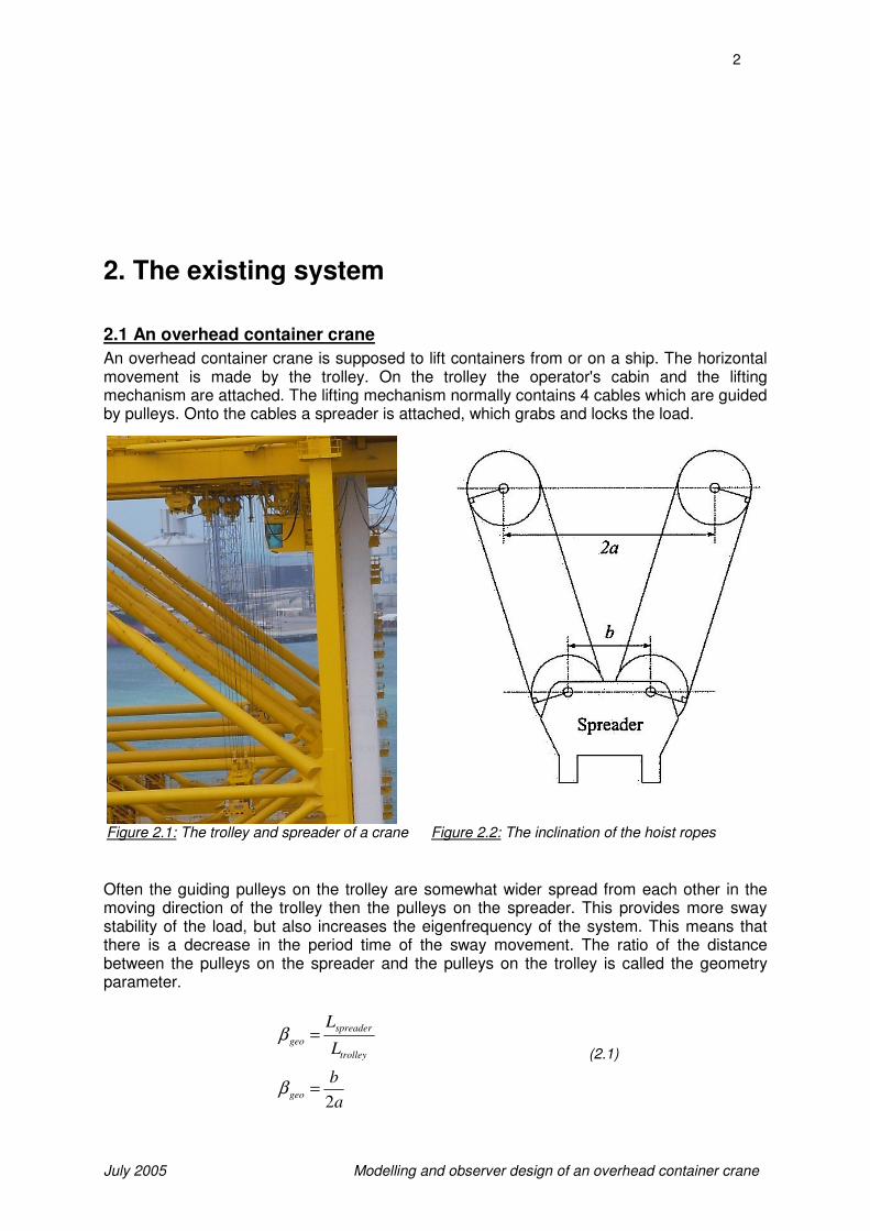
An overhead container crane is supposed to lift containers from or on a ship. The horizontal movement is made by the trolley. On the trolley the operator's cabin and the lifting mechanism are attached. The lifting mechanism normally contains 4 cables which are guided by pulleys. Onto the cables a spreader is attached, which grabs and locks the load.
Often the guiding pulleys on the trolley are somewhat wider spread from each other in the moving direction of the trolley then the pulleys on the spreader. This provides more sway stability of the load, but also increases the eigenfrequency of the system. This means that there is a decrease in the period time of the sway movement. The ratio of the distance between the pulleys on the spreader and the pulleys on the trolley is called the geometry parameter.
a
b
L
L
geo
trolley
spreader
geo
2=
=
β
β
(2.1)
Figure 2.1: The trolley and spreader of a crane Figure 2.2: The inclination of the hoist ropes

3
July 2005 Modelling and observer design of an overhead container crane
The closer this parameter is to zero, the lower the period time of the sway movement. For cranes with this configuration the model of the observer has to be designed. Only the newer
cranes, which are standard fitted with stabilizing controllers, have parallel cables ( 1≈geoβ ).
In table 2.1 the parameters used in the mathematical model of the crane are given. Table 2.1: The parameters used in the mathematical model
Mload 30000 kg Iy, load 45000 kgm2
Lload 0,8 m Ltrolley 1,3 m Hload 1,5 m k0, cable 20000 kNm-1
b0, cable 2000 kNsm-1
2.2 The Siemens observer
First the existing model for the observer now used in the HIPAC system is analyzed. The model used is that of a pendulum. XK (Xtrolley) is the input of the system. This is the trolley position controlled by the operator. PHL (φ) is the measured sway angle and is used as output of the master system, which is the real crane. In figure 2.3 the block diagram of this observer can be seen.
Figure 2.3: The block diagram of the observer model now implemented in HIPAC
The parameters h1, h2 and h3 are the gains of the observer and determined by optimalization. The block diagram contains the following equations:
( )L
XX loadtrolleyˆ
ˆsin−
=− ϕ (2.2)
4
July 2005 Modelling and observer design of an overhead container crane
( )ϕϕ ˆsinˆL
g−=&&
ϕ&&&&
ˆˆ LX load =
L
XXgX
loadtrolley
load
ˆˆ
−=
&&
(2.3)
ssXsX loadload
1)(ˆ)(ˆ ⋅=
&&& (2.4)
ssXsX loadload
1)(ˆ)(ˆ ⋅=
& (2.5)
With: ϕ̂ = estimated sway angle ( LHP ˆ )
Xtrolley = position of trolley (XK)
loadX̂ = estimated position of load ( LX ˆ )
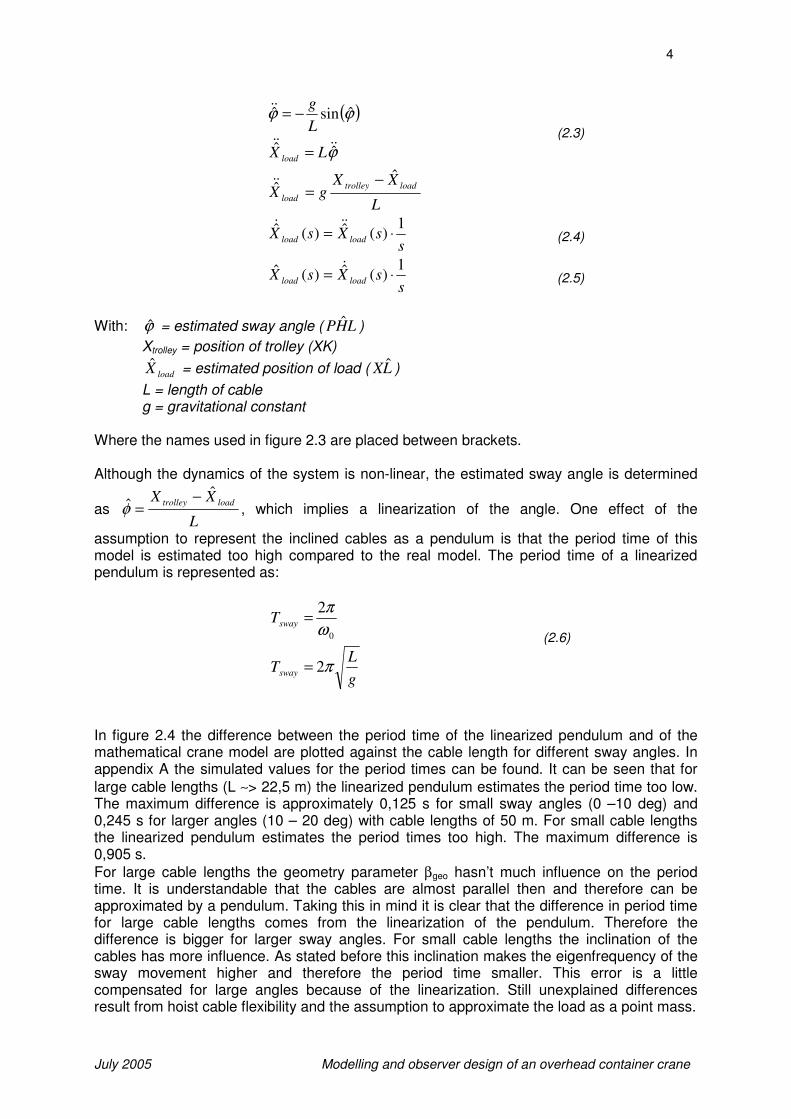
L = length of cable g = gravitational constant Where the names used in figure 2.3 are placed between brackets. Although the dynamics of the system is non-linear, the estimated sway angle is determined
as L
XX loadtrolleyˆ
ˆ−
=φ , which implies a linearization of the angle. One effect of the
assumption to represent the inclined cables as a pendulum is that the period time of this model is estimated too high compared to the real model. The period time of a linearized pendulum is represented as:
0
2
ω
π=swayT
g
LTsway π2=
(2.6)
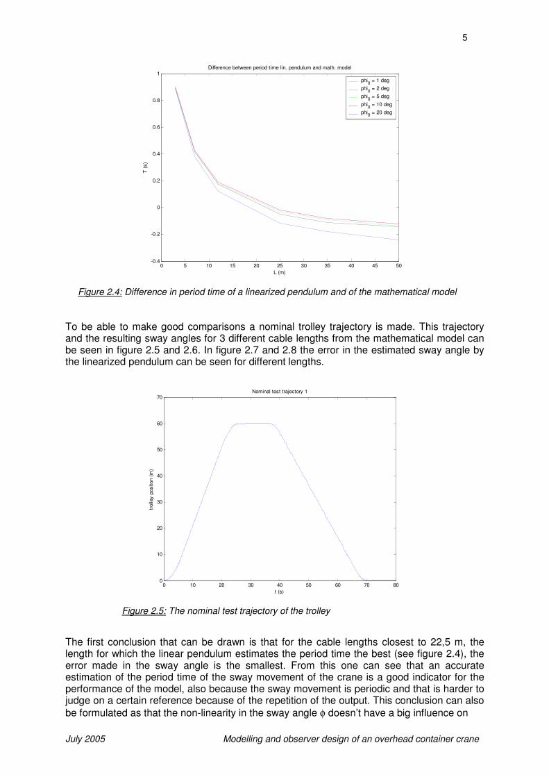
In figure 2.4 the difference between the period time of the linearized pendulum and of the mathematical crane model are plotted against the cable length for different sway angles. In appendix A the simulated values for the period times can be found. It can be seen that for
large cable lengths (L ∼> 22,5 m) the linearized pendulum estimates the period time too low. The maximum difference is approximately 0,125 s for small sway angles (0 –10 deg) and 0,245 s for larger angles (10 – 20 deg) with cable lengths of 50 m. For small cable lengths the linearized pendulum estimates the period times too high. The maximum difference is 0,905 s.
For large cable lengths the geometry parameter βgeo hasn’t much influence on the period time. It is understandable that the cables are almost parallel then and therefore can be approximated by a pendulum. Taking this in mind it is clear that the difference in period time for large cable lengths comes from the linearization of the pendulum. Therefore the difference is bigger for larger sway angles. For small cable lengths the inclination of the cables has more influence. As stated before this inclination makes the eigenfrequency of the sway movement higher and therefore the period time smaller. This error is a little compensated for large angles because of the linearization. Still unexplained differences result from hoist cable flexibility and the assumption to approximate the load as a point mass.
5
July 2005 Modelling and observer design of an overhead container crane
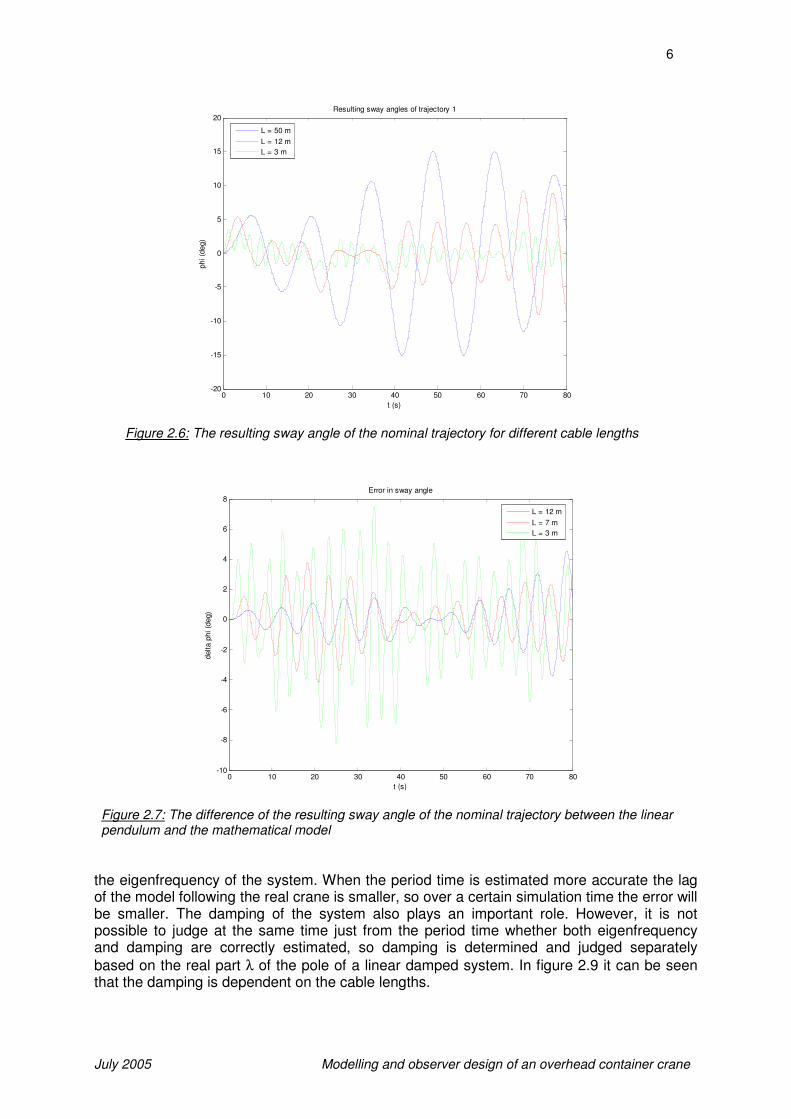
To be able to make good comparisons a nominal trolley trajectory is made. This trajectory and the resulting sway angles for 3 different cable lengths from the mathematical model can be seen in figure 2.5 and 2.6. In figure 2.7 and 2.8 the error in the estimated sway angle by the linearized pendulum can be seen for different lengths. The first conclusion that can be drawn is that for the cable lengths closest to 22,5 m, the length for which the linear pendulum estimates the period time the best (see figure 2.4), the error made in the sway angle is the smallest. From this one can see that an accurate estimation of the period time of the sway movement of the crane is a good indicator for the performance of the model, also because the sway movement is periodic and that is harder to judge on a certain reference because of the repetition of the output. This conclusion can also
be formulated as that the non-linearity in the sway angle φ doesn’t have a big influence on
0 5 10 15 20 25 30 35 40 45 50-0.4
-0.2
0
0.2
0.4
0.6
0.8
1Difference between period time lin. pendulum and math. model
L (m)
T (
s)
phi0 = 1 deg
phi0 = 2 deg
phi0 = 5 deg
phi0 = 10 deg
phi0 = 20 deg
Figure 2.4: Difference in period time of a linearized pendulum and of the mathematical model
0 10 20 30 40 50 60 70 800
10
20
30
40
50
60
70Nominal test trajectory 1
t (s)
trolley p
ositon (
m)
Figure 2.5: The nominal test trajectory of the trolley
6
July 2005 Modelling and observer design of an overhead container crane
0 10 20 30 40 50 60 70 80-20
-15
-10
-5
0
5
10
15
20Resulting sway angles of trajectory 1
t (s)
phi (d
eg)
L = 50 m
L = 12 m
L = 3 m
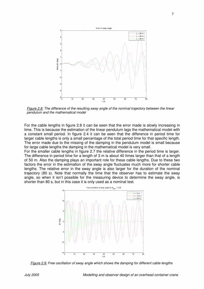
Figure 2.6: The resulting sway angle of the nominal trajectory for different cable lengths
0 10 20 30 40 50 60 70 80-10
-8
-6
-4
-2
0
2
4
6
8Error in sway angle
t (s)
delta p
hi (d
eg)
L = 12 m
L = 7 m
L = 3 m
Figure 2.7: The difference of the resulting sway angle of the nominal trajectory between the linear pendulum and the mathematical model
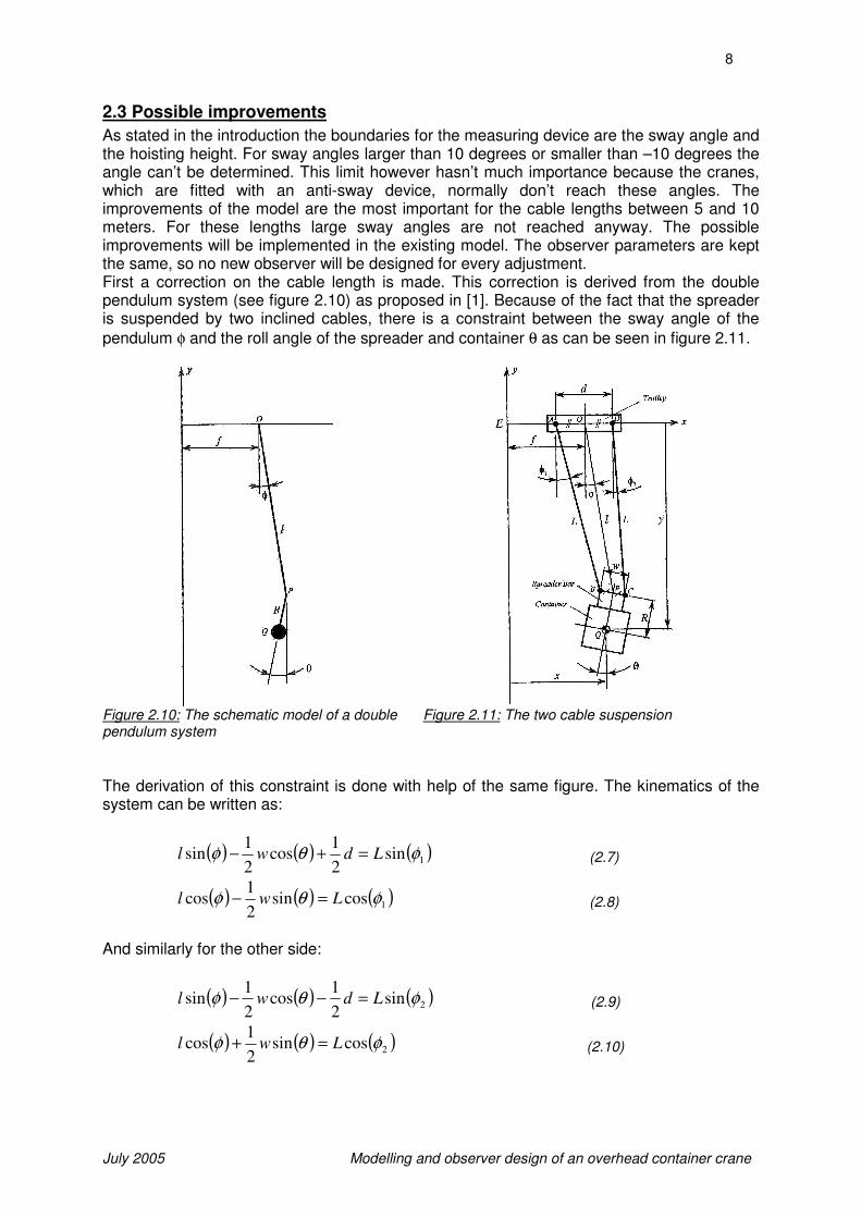
the eigenfrequency of the system. When the period time is estimated more accurate the lag of the model following the real crane is smaller, so over a certain simulation time the error will be smaller. The damping of the system also plays an important role. However, it is not possible to judge at the same time just from the period time whether both eigenfrequency and damping are correctly estimated, so damping is determined and judged separately
based on the real part λ of the pole of a linear damped system. In figure 2.9 it can be seen that the damping is dependent on the cable lengths.
7
July 2005 Modelling and observer design of an overhead container crane
For the cable lengths in figure 2.8 it can be seen that the error made is slowly increasing in time. This is because the estimation of the linear pendulum lags the mathematical model with a constant small period. In figure 2.4 it can be seen that the difference in period time for larger cable lengths is only a small percentage of the total period time for that specific length. The error made due to the missing of the damping in the pendulum model is small because for large cable lengths the damping in the mathematical model is very small. For the smaller cable lengths in figure 2.7 the relative difference in the period time is larger. The difference in period time for a length of 3 m is about 40 times larger than that of a length of 50 m. Also the damping plays an important role for these cable lengths. Due to these two factors the error in the estimation of the sway angle fluctuates much more for shorter cable lengths. The relative error in the sway angle is also larger for the duration of the nominal trajectory (80 s). Note that normally the time that the observer has to estimate the sway angle, so when it isn’t possible for the measuring device to determine the sway angle, is shorter than 80 s, but in this case it is only used as a nominal test.
0 10 20 30 40 50 60 70 80-15
-10
-5
0
5
10
15
Free oscillation of sway angle for Bgeo
= 0,35
t (s)
phi (d
eg)
L = 3 m
L = 12 m
L = 50 m
Figure 2.9: Free oscillation of sway angle which shows the damping for different cable lengths
0 10 20 30 40 50 60 70 80-5
-4
-3
-2
-1
0
1
2
3
4
5Error in sway angle
t (s)
delta
phi (d
eg
)
L = 50 m
L = 35 m
L = 25 m
Figure 2.8: The difference of the resulting sway angle of the nominal trajectory between the linear pendulum and the mathematical model
8
July 2005 Modelling and observer design of an overhead container crane
2.3 Possible improvements
As stated in the introduction the boundaries for the measuring device are the sway angle and the hoisting height. For sway angles larger than 10 degrees or smaller than –10 degrees the angle can’t be determined. This limit however hasn’t much importance because the cranes, which are fitted with an anti-sway device, normally don’t reach these angles. The improvements of the model are the most important for the cable lengths between 5 and 10 meters. For these lengths large sway angles are not reached anyway. The possible improvements will be implemented in the existing model. The observer parameters are kept the same, so no new observer will be designed for every adjustment. First a correction on the cable length is made. This correction is derived from the double pendulum system (see figure 2.10) as proposed in [1]. Because of the fact that the spreader is suspended by two inclined cables, there is a constraint between the sway angle of the
pendulum φ and the roll angle of the spreader and container θ as can be seen in figure 2.11.
Figure 2.10: The schematic model of a double pendulum system
Figure 2.11: The two cable suspension
The derivation of this constraint is done with help of the same figure. The kinematics of the system can be written as:
( ) ( ) ( )1sin2
1cos
2
1sin φθφ Ldwl =+− (2.7)
( ) ( ) ( )1cossin2
1cos φθφ Lwl =− (2.8)
And similarly for the other side:
( ) ( ) ( )2sin2
1cos
2
1sin φθφ Ldwl =−− (2.9)
( ) ( ) ( )2cossin2
1cos φθφ Lwl =+ (2.10)
9
July 2005 Modelling and observer design of an overhead container crane
Squaring and adding (2.7) and (2.8) and (2.9) and (2.10) yields:
( ) ( ) ( ) ( ) 2
22
2
1cos
2
1sinsin
2
1cos Ldwlwl =
+−+
− θφθφ (2.11)
( ) ( ) ( ) ( ) 2
22
2
1cos
2
1sinsin
2
1cos Ldwlwl =
−−+
+ θφθφ (2.12)
By eliminating L2 from (2.11) and (2.12) and manipulating the result the following relation
between φ and θ is obtained:
( ) ( )φθφ += sinsin wd (2.13)
Which can be written when linearized for small angles as:
φθw
wd −= (2.14)
From figure 2.11 it can be seen that the following holds:
φθ lRxx lk +−= (2.15)
This equation replaces (2.2) in the original model. The pendulum length l depends on cable
length L, trolley width d, spreader width w and sway angle φ. The relation for l is found by simplifying (2.12) using equation (2.14):
−−+−= φ
wd
wdwwdLl cos2
4
1 2222 (2.16)
which for small oscillations reduces to:
( )222
4
1wdLl −−= (2.17)
Now using (2.14) and (2.17) in (2.15) yields:
( ) φφ
−−+
−−=
22
4
1wdL
w
wdRxx lk
( )
−−−−
−=
w
wdRwdL
xx lk
22
4
1φ
(2.18)
And then the following holds for the period time:
( )
g
w
wdRwdL
T
−−−−
=
22
4
1
2π (2.19)

10
July 2005 Modelling and observer design of an overhead container crane
The term
−
w
wdR can be seen as a correction on the pendulum length which
compensates the roll and the corresponding motion of the center of gravity of the container for a two cable suspension.
With the correction made for the pendulum length the effect of βgeo from (2.1) on the period
time can be visualised (see figure 2.12). As stated before a lower βgeo decreases the period
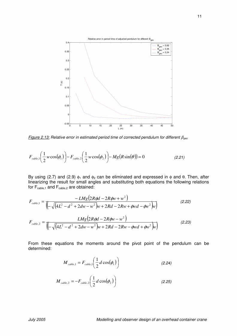
time, in particular for small cable lengths. For βgeo = 0,24 a period time for L = 3 m couldn’t be obtained, because the cable length became non-positive due to the corrections made. The comparison in figure 2.4 with the uncorrected pendulum was done for a βgeo of 0,62. In comparison with the blue line in figure 2.12 this line is shifted down a little. This makes the model worse for large cable lengths, but for the shorter lengths, which are the most important, it performs better. This is clearly understandable, because the pendulum length is corrected for the constraints due to the inclined two cable suspension, and the inclination is largest, and thus has the most influence, when the cable lengths are small. In figure 2.13 the relative error, which is the difference between the period time of the adjusted pendulum minus the period time of the mathematical model divided by he same period time of the mathematical model, made in the estimation of the period time by the pendulum with adjusted length compared to the mathematical model is plotted. It can be seen that for the large cable lengths the error stays below 5%, but for the shorter cable
lengths the error increases up to 40% for βgeo = 0,24.
Another possibility to explain the decrease in the period time with increasing βgeo is by the cable forces that introduce an extra moment around the pivot point of the pendulum due to the inclination of the cables. It is tried to compensate this moment. First the static forces in the cables are determined. This is done by formulating the static force- and moment equilibrium from figure 2.11:
0 5 10 15 20 25 30 35 40 45 500
5
10
15
Period time of adjusted pendulum (solid) and mathematical model (dotted) for different Bgeo
L (m)
T (
s)
Bgeo
= 0,62
Bgeo
= 0,35
Bgeo
= 0,24
Figure 2.12: Period time for the corrected pendulum (solid) and mathematical model (dotted) for
different βgeo
( ) ( ) 0coscos 22,11, =−+ MgFF cablecable φφ (2.20)
11
July 2005 Modelling and observer design of an overhead container crane
By using (2.7) and (2.9) φ1 and φ2 can be eliminated and expressed in φ and θ. Then, after linearizing the result for small angles and substituting both equations the following relations for Fcable,1 and Fcable,2 are obtained:
( )( )( )( )wwwdRwRdwwdwdL
wwRdRLMgFcable
2222
2
1,
2224
22
φφ
φφ
−+−+−+−−
+−−= (2.22)
( )( )( )( )wwwdRwRdwwdwdL
wwRdRLMgFcable
2222
2
2,
2224
22
φφ
φφ
+−−+−+−−
−−= (2.23)
From these equations the moments around the pivot point of the pendulum can be determined:
( )
= 11,1, cos
2
1φdFM cablecable (2.24)
( )
−= 22,2, cos
2
1φdFM cablecable (2.25)
0 5 10 15 20 25 30 35 40 45 50-0.05
0
0.05
0.1
0.15
0.2
0.25
0.3
0.35
0.4
Relative error in period time of adjusted pendulum for different Bgeo
L (m)
T (
s)
Bgeo
= 0,62
Bgeo
= 0,35
Bgeo
= 0,24
Figure 2.13: Relative error in estimated period time of corrected pendulum for different βgeo
( ) ( ) ( )( ) 0sincos2
1cos
2
122,11, =−
−
θφφ RMgwFwF cablecable (2.21)
12
July 2005 Modelling and observer design of an overhead container crane
Again by using (2.7) and (2.9) the following relations for Mcable,1 and Mcable,2 are obtained:
( )2
2
1,4
22
w
wwRdRdMgM cable
+−=
φφ (2.26)
( )2
2
2,4
22
w
wwRdRdMgM cable
−−=
φφ (2.27)
For the resulting moment around the pendulum pivot point it then follows:
( )φ
2
2,1,
w
wdgMdRM
MMM
cable
cablecablecable
−=∆
+=∆
(2.28)
It can be seen that there exists a linear relation between the resulting moment and the
pendulum sway angle φ. Therefore this moment can be represented in the mass normalised linear pendulum model by a torsional spring with stiffness:
( )22
Lw
wdgdRk torsion
−= (2.29)
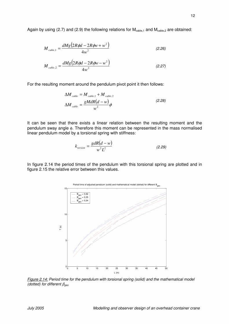
In figure 2.14 the period times of the pendulum with this torsional spring are plotted and in figure 2.15 the relative error between this values.
0 5 10 15 20 25 30 35 40 45 500
5
10
15
Period time of adjusted pendulum (solid) and mathematical model (dotted) for different Bgeo
L (m)
T (
s)
Bgeo
= 0,62
Bgeo
= 0,35
Bgeo
= 0,24
Figure 2.14: Period time for the pendulum with torsional spring (solid) and the mathematical model
(dotted) for different βgeo

13
July 2005 Modelling and observer design of an overhead container crane
0 5 10 15 20 25 30 35 40 45 50-0.15
-0.1
-0.05
0
0.05
0.1
0.15
0.2
0.25
0.3
Relative error in period time of adjusted pendulum for different Bgeo
L (m)
T (
s)
Bgeo
= 0,62
Bgeo
= 0,35
Bgeo
= 0,24
Figure 2.15: The relative error in the estimated period time of the pendulum with torsional spring for
different βgeo
The relative errors for this adjustment are smaller for short cable lengths than that of the pendulum length correction. For the larger lengths however it will perform worse. But because the range between 5 and 10 meters is the most important, it can be concluded that this model is better. There are now two adjustments to the linear model presented which will correct the period time based on the physical kinematics of the system. In section 3.2 also a semi-empirical way is presented. Other linear adjustments based on physical background couldn’t be found. The period time however still isn’t estimated correctly due to the flexibility of the cables and there is also no damping introduced in the pendulum. To account for these two parameters in the right way an empirical approach can be used. By adding extra torsional stiffness and damping in the pivot point the period time and damping can be fitted exactly onto that of the real crane. The stiffness and damping will be dependent on the parameters which describe the kinematics of the system and the cable stiffness and damping, and are determined by fitting measurement data. There are also several other influences on the damping like the flexibility of the total construction and the air resistance of the container. Because there is no real physical explanation for the values of the fictive torsional stiffness and damping, they are determined purely empirical, it is questionable how this mapping will work on different cranes. Of course every crane is different and so every crane has to be tested separately to be able to make a good mapping, while a purely physical model will work on every crane because the basics are the same. Determining the stiffness can be done by using the difference in period time of the used estimation model and the real crane for different cable lengths, geometry parameters and cable properties. Obtaining the damping parameter can be done by analysing the free sway movement of the crane for different cable lengths and geometry parameters. Thereby the assumption is made that the system is weakly damped. Then by making an exponential fit through the peaks of the oscillations the real part of the pole of the system can be determined. See figure 2.16 and (2.30) and (2.31). A free sway movement can be established by a sudden (de)-acceleration of the trolley and then keeping a constant velocity.

14
July 2005 Modelling and observer design of an overhead container crane
0 5 10 15 20 25 30-3
-2
-1
0
1
2
3
4Check whether it is good fit
t (s)
phi (d
eg)
swayangle
fit of dampingcoefficient
Figure 2.16: Exponential fit of tops of oscillations to obtain damping coefficient
For the red line it holds that:
( )( ) ( )nTttettt +=== 00 φφ λ
,
with T
tn max,...,2,1=
(2.30)
and then by using the least squares method λ is determined. For the damping coefficient it holds that: With: t0 = time of first maximum T = period time n = number of periods in measurement
λ = real part of pole of system d = damping coefficient
To avoid unreliable λ-values only the maxima of the oscillations are used which are larger than 10% of the highest maximum value, because the low values are very sensitive to noise and errors. The damping normally has influence on the eigenfrequency, and therefore also on the period time:
( )λ22 lMd load−= (2.31)
)1(2ξωω −= nd ,
with nω
λξ −=
(2.32)
15
July 2005 Modelling and observer design of an overhead container crane
This equation only holds for weakly damped systems. But because ξ is very small for most combinations of the important parameters this effect is negligible.
As said above the damping coefficient is obtained by determining λ. This is the real part of the pole of the system. However, when using this, a linear transfer function for the system is
assumed. As appeared from the fitting procedure of λ the regression was good, except for
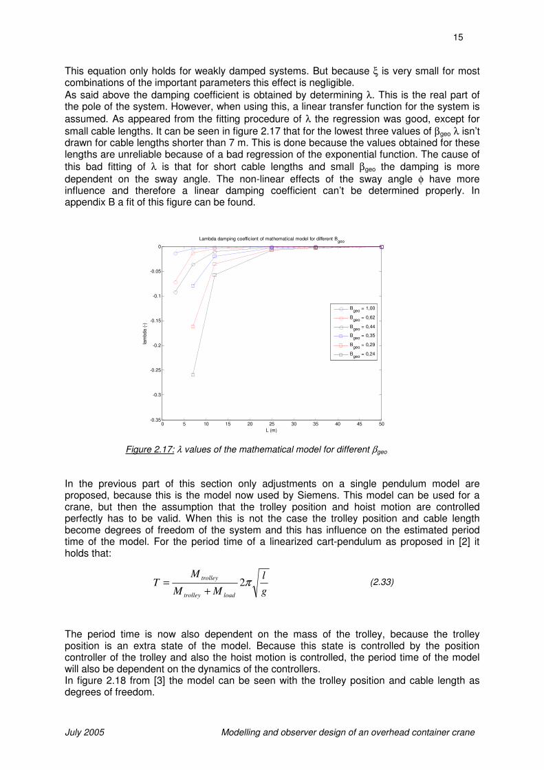
small cable lengths. It can be seen in figure 2.17 that for the lowest three values of βgeo λ isn’t drawn for cable lengths shorter than 7 m. This is done because the values obtained for these lengths are unreliable because of a bad regression of the exponential function. The cause of
this bad fitting of λ is that for short cable lengths and small βgeo the damping is more
dependent on the sway angle. The non-linear effects of the sway angle φ have more influence and therefore a linear damping coefficient can’t be determined properly. In appendix B a fit of this figure can be found.
0 5 10 15 20 25 30 35 40 45 50-0.35
-0.3
-0.25
-0.2
-0.15
-0.1
-0.05
0
Lambda damping coefficient of mathematical model for different Bgeo
L (m)
lam
bda (
-)
Bgeo
= 1,00
Bgeo
= 0,62
Bgeo
= 0,44
Bgeo
= 0,35
Bgeo
= 0,29
Bgeo
= 0,24
Figure 2.17: λ values of the mathematical model for different βgeo
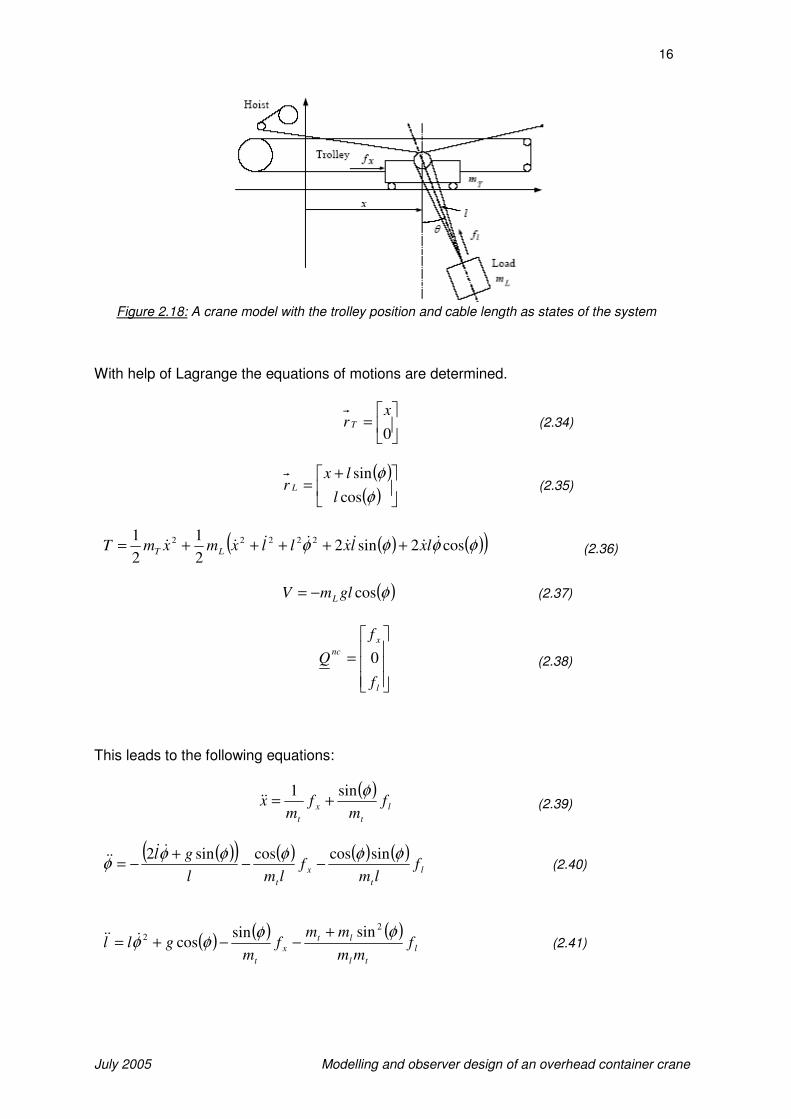
In the previous part of this section only adjustments on a single pendulum model are proposed, because this is the model now used by Siemens. This model can be used for a crane, but then the assumption that the trolley position and hoist motion are controlled perfectly has to be valid. When this is not the case the trolley position and cable length become degrees of freedom of the system and this has influence on the estimated period time of the model. For the period time of a linearized cart-pendulum as proposed in [2] it holds that: The period time is now also dependent on the mass of the trolley, because the trolley position is an extra state of the model. Because this state is controlled by the position controller of the trolley and also the hoist motion is controlled, the period time of the model will also be dependent on the dynamics of the controllers. In figure 2.18 from [3] the model can be seen with the trolley position and cable length as degrees of freedom.
g
l
MM
MT
loadtrolley
trolleyπ2
+= (2.33)
16
July 2005 Modelling and observer design of an overhead container crane
Figure 2.18: A crane model with the trolley position and cable length as states of the system
With help of Lagrange the equations of motions are determined.
=
0
xr T (2.34)
( )( )
+=
φ
φ
cos
sin
l
lxr L (2.35)
( ) ( )( )φφφφ cos2sin22
1
2
1 22222 &&&&&&&& lxlxllxmxmT LT +++++= (2.36)
( )φcosglmV L−= (2.37)
=
l
x
nc
f
f
Q 0 (2.38)
This leads to the following equations:
( )l
t
x
t
fm
fm
xφsin1
+=&& (2.39)
( )( ) ( ) ( ) ( )l
t
x
t
flm
flml
gl φφφφφφ
sincoscossin2−−
+−=
&&&& (2.40)
( ) ( ) ( )l
tl
lt
x
t
fmm
mmf
mgll
φφφφ
2
2 sinsincos
+−−+= &&& (2.41)

17
July 2005 Modelling and observer design of an overhead container crane
Now a coordinate transformation is chosen:
xz =1
xz &=2
( )φsin3 =z
( )φφ cos4&=z
lz =5
lz &=6
(2.51)
This leads to the following state equations:
21 zz =&
32
1z
m
ff
mz
t
l
x
t
+=&
( )φφ cos3&& =z
43 zz =&
( ) ( )
( )( ) ( ) ( ) ( ) ( ) ( )φφφφφφφφ
φφφφ
sincossincoscossin2
sincos
2
2
4
&&&
&&&&
−
−−
+−=
−=
l
t
x
t
flm
flml
gl
z
( ) ( )2
3
2
432
33
5
2
3
5
2
33
5
4
5
6
41
1112
z
zzzz
zm
fz
zm
fzz
z
gz
z
zz
t
l
t
x
−−−−−−−−−=&
65 zz =&
2
33
2
32
3
2
4
56 11
zmm
fmf
mm
mz
m
fzg
z
zzz
tl
ll
l
tl
t
t
x −−−−+−
=&
(2.52)
The output of the system is:
=
6
5
3
2
1
z
z
z
z
z
y
(2.53)
The observability of a non-linear system normally can be checked by constructing the observability matrix:
( )( )
( )
=
=Φ
−xhL
xhL
xhy
n
f
f
1
M
M
(2.54)
18
July 2005 Modelling and observer design of an overhead container crane
Then by looking to the rank of the jacobian x∂
Φ∂ the local observability can be determined.
However, because this system is 6th order system and contains many non-linear terms the construction of the observability matrix is very complicated. Therefore, because the system physically shows a large similarity with a pendulum, the system is compared with a linear pendulum, and because a linear pendulum is observable it is assumed that the non-linear system is also observable. This can also be checked afterwards by simulation.
Because x , x& , l , l& ( 1z , 2z , 5z , 6z ), the trolley driving force fx and the lifting force fl are
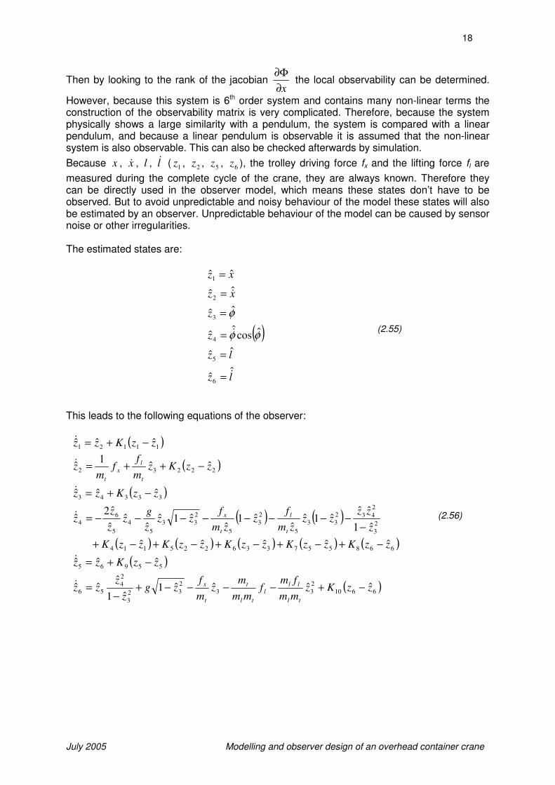
measured during the complete cycle of the crane, they are always known. Therefore they can be directly used in the observer model, which means these states don’t have to be observed. But to avoid unpredictable and noisy behaviour of the model these states will also be estimated by an observer. Unpredictable behaviour of the model can be caused by sensor noise or other irregularities. The estimated states are:
( )
lz
lz
z
z
xz
xz
ˆˆ
ˆˆ
ˆcosˆ
ˆ
ˆˆ
ˆˆ
ˆˆ
6
5
4
3
2
1
&
&
&
=
=
=
=
=
=
φφ
φ
(2.55)
This leads to the following equations of the observer:
( )11121ˆˆˆ zzKzz −+=&
( )22232
ˆˆ1
ˆ zzKzm
ff
mz
t
l
x
t
−++=&
( )33343
ˆˆˆ zzKzz −+=&
( ) ( )
( ) ( ) ( ) ( ) ( )668557336225114
2
3
2
432
33
5
2
3
5
2
33
5
4
5
6
4
ˆˆˆˆˆ
ˆ1
ˆˆˆ1ˆ
ˆˆ1
ˆˆ1ˆ
ˆˆ
ˆ
ˆ2ˆ
zzKzzKzzKzzKzzK
z
zzzz
zm
fz
zm
fzz
z
gz
z
zz
t
l
t
x
−+−+−+−+−+
−−−−−−−−−=&
( )55965
ˆˆˆ zzKzz −+=&
( )6610
2
33
2
32
3
2
4
56ˆˆˆˆ1
ˆ1
ˆˆˆ zzKz
mm
fmf
mm
mz
m
fzg
z
zzz
tl
ll
l
tl
t
t
x −+−−−−+−
=&
(2.56)
19
July 2005 Modelling and observer design of an overhead container crane
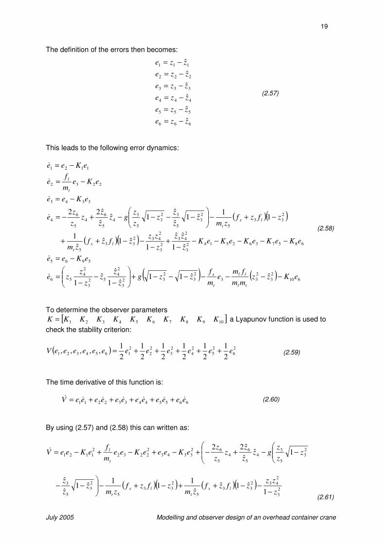
The definition of the errors then becomes: This leads to the following error dynamics:
1121 eKee −=&
2232 eKem
fe
t
l −=&
3343 eKee −=&
( )( )2
33
5
2
3
5
32
3
5
3
4
5
6
4
5
6
4 11
ˆ1ˆ
ˆ1ˆ
ˆ
ˆ22zfzf
zmz
z
zz
z
zgz
z
zz
z
ze lx
t
−+−
−−−−+−=&
( )( ) 68573625142
3
2
43
2
3
2
432
33
5ˆ1
ˆˆ
1ˆ1ˆ
ˆ
1eKeKeKeKeK
z
zz
z
zzzfzf
zmlx
t
−−−−−−
+−
−−++
5965 eKee −=&
( ) ( )610
2
3
2
33
2
3
2
32
3
2
4
52
3
2
4
56ˆˆ11
ˆ1
ˆˆ
1eKzz
mm
fme
m
fzzg
z
zz
z
zze
tl
ll
t
x −−−−−−−+
−−
−=&
(2.58)
To determine the observer parameters
[ ]10987654321 KKKKKKKKKKK = a Lyapunov function is used to
check the stability criterion:
The time derivative of this function is:
665544332211 eeeeeeeeeeeeV &&&&&&& +++++= (2.60)
By using (2.57) and (2.58) this can written as:
−−+−+−+−+−= 2
3
5
3
4
5
6
4
5
62
3343
2
2232
2
1121 1ˆˆ
ˆ22z
z
zgz
z
zz
z
zeKeeeKee
m
feKeeV
t
l&
( )( ) ( )( )2
3
2
432
33
5
2
33
5
2
3
5
3
1ˆ1ˆ
ˆ
11
1ˆ1
ˆ
ˆ
z
zzzfzf
zmzfzf
zmz
z
zlx
t
lx
t −−−++−+−
−−
(2.61)
666
555
444
333
222
111
ˆ
ˆ
ˆ
ˆ
ˆ
ˆ
zze
zze
zze
zze
zze
zze
−=
−=
−=
−=
−=
−=
(2.57)
( ) 2
6
2
5
2
4
2
3
2
2
2
16543212
1
2
1
2
1
2
1
2
1
2
1,,,,, eeeeeeeeeeeeV +++++= (2.59)

20
July 2005 Modelling and observer design of an overhead container crane
( ) ( ) 6
2
3
2
3636
2
3
2
362
3
2
4
52
3
2
4
5
2
5965468573625142
3
2
43
ˆˆ11ˆ1
ˆˆ
1
ˆ1
ˆˆ
ezzmm
fmee
m
fezzge
z
zz
z
zz
eKeeeeKeKeKeKeKz
zz
tl
ll
t
x −−−−−−+
−−
−
+−+
−−−−−
−+
2
610eK−
Because a trolley moves over a boom of a certain length, the position of the trolley is limited
between 0 and the length of the boom (Lboom ≈ 100 m). Therefore it holds that: 1000 1 ≤≤ z .
For z2, the trolley velocity, there are also limits. Because the driving engine has a limited maximum rpm and the gear ratios are known a maximum trolley velocity can be determined.
This velocity is 3,5 ms-1, so it holds that: 5.35,3 2 ≤≤− z . Due to the application of an anti
sway system, the inclined cables and a limited acceleration of the trolley the sway angle of
the load will normally not exceed 15 degrees. So for z3 it holds that: 262,0262,0 3 ≤≤− z . By
doing some simulations with the maximum trolley acceleration (max(aT) ≈ 0,7 ms-2) the maximum sway angle velocity is determined at approximately 1 rads-1. This means that for z4
it holds that: 940,0940,0 4 ≤≤− z . Of course the cable length is also limited and depends on
the height of the crane. Normally this height is approximately 50 m. Next to that, the inclined cables are the cause of the fact that the cable length also has a minimum. This minimum is
approximately 3 m. So for z5 it can be concluded that: 503 5 ≤≤ z . The engine that drives the
hoist motion also has a limited maximum rpm. For a crane this means that the maximum hoist velocity, with an empty spreader, is 2,5 ms-1. Therefore for z6 it holds that:
5,25,2 6 ≤≤− z . The maximum drive force of the trolley fx is approximately 50 kN and the
hoist force fl is 417 kN. Using this information and the assumption that these limits also hold for the estimated states of the observer, a worst case value can be obtained for the terms in (2.61). Then by choosing the correct observer parameters (2.61) will be negative definite for all errors within a feasible domain. Because the Lyapunov function of (2.61) is very complicated in this case, the explicit description of this problem is not given here. But if the observer parameters are chosen large enough the negative quadratic terms will compensate for the other terms and will make the Lyapunov function negative definite for the total error domain.
21
July 2005 Modelling and observer design of an overhead container crane
3. Alternative models
3.1 Linearized double pendulum
The double pendulum model, which can be seen in figure 2.9, is already used to derive the cable length correction for the linear pendulum. For the double pendulum however also the linearized equations of motion can be derived. This is done in [1] and also contains the constraints as described in section 2.3 of this report. This leads to the following linearized equation of motion:
( )( )
( )0
2
2
=−
++
−+ φφ
aRl
Ralg
aRL
f&&&& (3.1)
With: xf &&&& =
( )22
4
1wdLl −−=
w
wda
−=
And then the period time is:
( )( )Ralg
aRlT
2
2
2+
−= π (3.2)
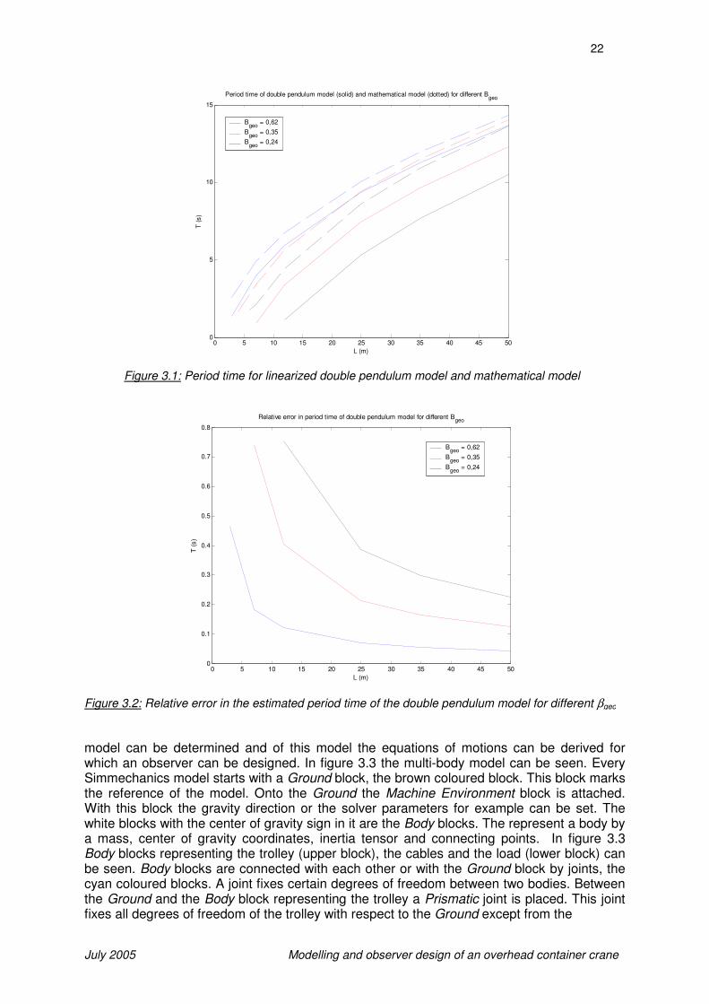
In figure 3.1 the period time for this model is plotted against the cable length L together with the period time for the mathematical model for different geometry parameters. It can be seen that the period time is estimated too low, especially for the, important, short cable lengths. This model performs worse than the two adjusted linear pendulums proposed in the previous chapter. Like these two models it also lacks damping, which only can be added by empirical ways.
3.2 Two cable suspension
In figure 2.2 and 2.10 the configuration of a two cable suspension could be seen. From [1] and [4] it can be concluded that the derivation of the equations of motion of this configuration is time consuming and complex. Therefore first a multi-body model with help of Simmechanics is made to test the model and possible adapted versions. Within Simmechanics it is very easy to make adjustments in the model or its parameters without having to derive the equations of motions over again. After the simulation tests the best
22
July 2005 Modelling and observer design of an overhead container crane
model can be determined and of this model the equations of motions can be derived for which an observer can be designed. In figure 3.3 the multi-body model can be seen. Every Simmechanics model starts with a Ground block, the brown coloured block. This block marks the reference of the model. Onto the Ground the Machine Environment block is attached. With this block the gravity direction or the solver parameters for example can be set. The white blocks with the center of gravity sign in it are the Body blocks. The represent a body by a mass, center of gravity coordinates, inertia tensor and connecting points. In figure 3.3 Body blocks representing the trolley (upper block), the cables and the load (lower block) can be seen. Body blocks are connected with each other or with the Ground block by joints, the cyan coloured blocks. A joint fixes certain degrees of freedom between two bodies. Between the Ground and the Body block representing the trolley a Prismatic joint is placed. This joint fixes all degrees of freedom of the trolley with respect to the Ground except from the
0 5 10 15 20 25 30 35 40 45 500
0.1
0.2
0.3
0.4
0.5
0.6
0.7
0.8
Relative error in period time of double pendulum model for different Bgeo
L (m)
T (
s)
Bgeo
= 0,62
Bgeo
= 0,35
Bgeo
= 0,24
Figure 3.2: Relative error in the estimated period time of the double pendulum model for different βgeo
0 5 10 15 20 25 30 35 40 45 500
5
10
15
Period time of double pendulum model (solid) and mathematical model (dotted) for different Bgeo
L (m)
T (
s)
Bgeo
= 0,62
Bgeo
= 0,35
Bgeo
= 0,24
Figure 3.1: Period time for linearized double pendulum model and mathematical model

23
July 2005 Modelling and observer design of an overhead container crane
translation in the x-direction. In reality this translation is the movement of the trolley from ship to shore and vice versa. The motion of the trolley is controlled by a PD-controller. This controller is fast enough to track the prescribed motion without any difference compared to the mathematical model. Between the trolley and the cables Revolute joints are placed. These joints restrict every movement of the cables with respect to the trolley except from the rotation about the y-axis. As can be seen in figure 3.3 each cable consists of two Body blocks. This is done to be able to make the cables shorter or longer during simulation to simulate hoisting movements. Between these two Bodies a Prismatic joint is placed with the translation movement in the local z-direction of the cables as degree of freedom. With the red coloured Joint Actuators the hoisting of the cables is then prescribed to this joint. The other red blocks are also Actuators or Sensors which measure a position or velocity of a Body or Joint. Finally the cables are attached to the Body block representing the load by Revolute joints with the rotation about the y-axis as degree of freedom. The two green blocks apply an initial position and velocity to the trolley and an initial sway angle and sway angle velocity to cable 2 (and due to the kinematics of the system also automatically to cable 1). These are normally set to zero. The small blue blocks are the inputs and outputs of the system. There are two inputs, the position of the trolley and the hoisting height, and four outputs, the
position of the trolley, the sway angle of the fictive pendulum (which can be seen as angle φ in figure 2.10), and the sway angle and sway angle velocity of cable 1. The last two outputs can be seen as the states of the system. With these two states the total model can be described. The sway angle of the fictive pendulum is:
4
x(2) - Sway angle speed cable 1 (degs-1)
3
x(1) - Sway angle cable 1 (deg)
2
y(2) - Sway angle pendulum (deg)
1
y(1) - Horizontal position trolley (m)
CS
1
CS
2
CS
3
CS
4
CS
5
T rol ley
In1Out1
Subsystem2
In1Out1
Subsystem1
BF
Revolute2b
B
F
Revolute2a
BF
Revolute1b
B
F
Revolute1a
B
F
Prismatic3
B
F
Prismatic2B
F
Prismatic1
In1Out1
PD-control ler
Env
Machine
Environment
CS
1
CS
2
CS
3
Load (headblock, spreader, container)
Joint Sensor1
Joint Actuator1 Joint Actuator
Initial trolley conditions
Initial sway conditions
Ground
[trolley_pv]Goto1
[spreader_pv]Goto
[spreader_pv]
From1
[trol ley_pv]
From
u(1)
Fcn2
f(u)
Fcn1
u(1)
Fcn
0
Constant
CS
1C
S2
Cable 2bC
S1
CS
2
Cable 2a
L02Cable 2 ini tial length
CS
1C
S2
Cable 1b
CS
1C
S2
Cable 1aL01Cable 1 ini tial length
Body Sensor1
Body Sensor
Body Actuator
2
u(3) - Length of cables (m)
1
u(1) Position trolley
Figure 3.3: The multi-body model of the two cable suspension crane in Simmechanics
−
−=
load
loadtrolley
pendZ
XXarctanφ (3.3)
24
July 2005 Modelling and observer design of an overhead container crane
With: pendφ = sway angle of fictive pendulum
trolleyX = position of trolley (measured in the middle of the trolley)
loadX = horizontal position of load (measured in the middle of the spreader)
loadZ = vertical position of load (measured in the middle of the spreader)
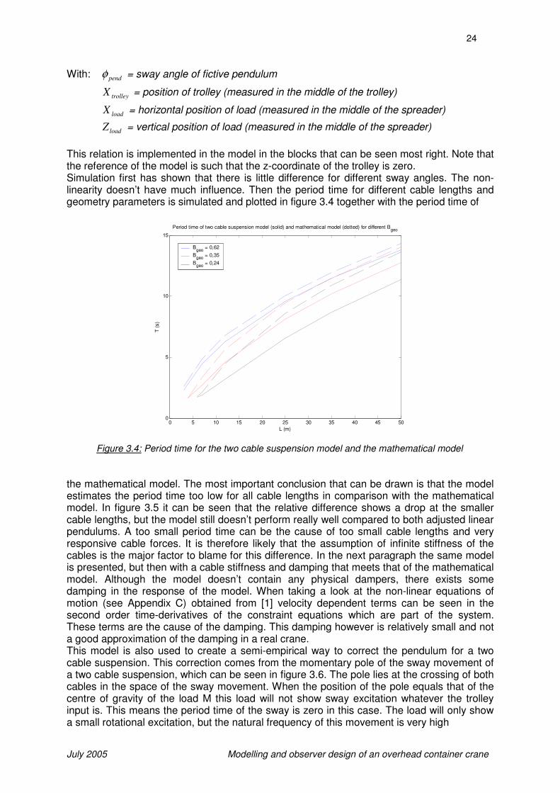
This relation is implemented in the model in the blocks that can be seen most right. Note that the reference of the model is such that the z-coordinate of the trolley is zero. Simulation first has shown that there is little difference for different sway angles. The non-linearity doesn’t have much influence. Then the period time for different cable lengths and geometry parameters is simulated and plotted in figure 3.4 together with the period time of
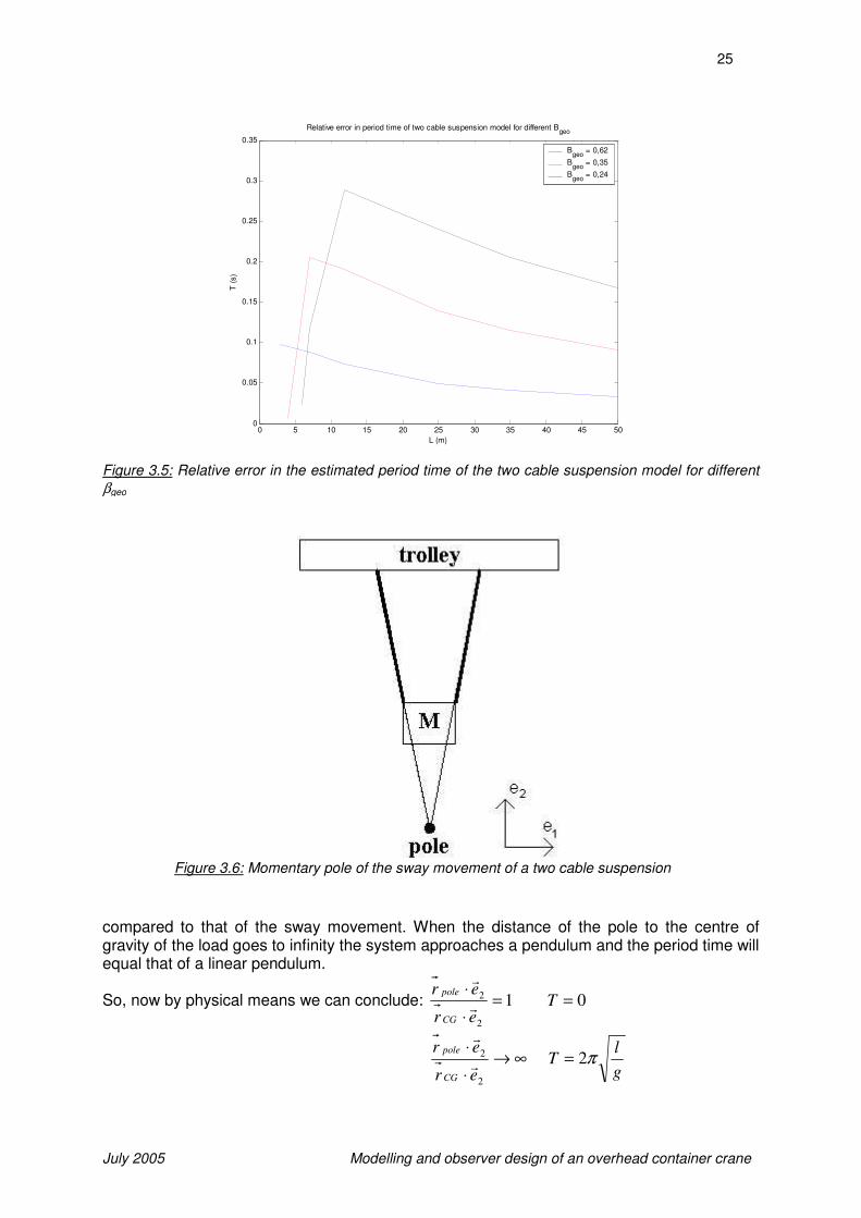
the mathematical model. The most important conclusion that can be drawn is that the model estimates the period time too low for all cable lengths in comparison with the mathematical model. In figure 3.5 it can be seen that the relative difference shows a drop at the smaller cable lengths, but the model still doesn’t perform really well compared to both adjusted linear pendulums. A too small period time can be the cause of too small cable lengths and very responsive cable forces. It is therefore likely that the assumption of infinite stiffness of the cables is the major factor to blame for this difference. In the next paragraph the same model is presented, but then with a cable stiffness and damping that meets that of the mathematical model. Although the model doesn’t contain any physical dampers, there exists some damping in the response of the model. When taking a look at the non-linear equations of motion (see Appendix C) obtained from [1] velocity dependent terms can be seen in the second order time-derivatives of the constraint equations which are part of the system. These terms are the cause of the damping. This damping however is relatively small and not a good approximation of the damping in a real crane. This model is also used to create a semi-empirical way to correct the pendulum for a two cable suspension. This correction comes from the momentary pole of the sway movement of a two cable suspension, which can be seen in figure 3.6. The pole lies at the crossing of both cables in the space of the sway movement. When the position of the pole equals that of the centre of gravity of the load M this load will not show sway excitation whatever the trolley input is. This means the period time of the sway is zero in this case. The load will only show a small rotational excitation, but the natural frequency of this movement is very high
0 5 10 15 20 25 30 35 40 45 500
5
10
15
Period time of two cable suspension model (solid) and mathematical model (dotted) for different Bgeo
L (m)
T (
s)
Bgeo
= 0,62
Bgeo
= 0,35
Bgeo
= 0,24
Figure 3.4: Period time for the two cable suspension model and the mathematical model
25
July 2005 Modelling and observer design of an overhead container crane
compared to that of the sway movement. When the distance of the pole to the centre of gravity of the load goes to infinity the system approaches a pendulum and the period time will equal that of a linear pendulum.
So, now by physical means we can conclude: 01
2
2 ==⋅
⋅T
er
er
CG
pole
r
r
g
lT
er
er
CG
poleπ2
2
2 =∞→⋅
⋅r
r
0 5 10 15 20 25 30 35 40 45 500
0.05
0.1
0.15
0.2
0.25
0.3
0.35
Relative error in period time of two cable suspension model for different Bgeo
L (m)
T (
s)
Bgeo
= 0,62
Bgeo
= 0,35
Bgeo
= 0,24
Figure 3.5: Relative error in the estimated period time of the two cable suspension model for different
βgeo
Figure 3.6: Momentary pole of the sway movement of a two cable suspension

26
July 2005 Modelling and observer design of an overhead container crane
where polerr
is the position vector of the pole and CGrr
is the position vector of the centre of
gravity of the load. The root of both vectors lies in the centre of the trolley. Using the above shown points it can be concluded that the relation between the period time and the distance ratio looks like:
( ))1(12
−−−= xC
g
lT π (3.4)
where C is a constant and
2
2
er
erx
CG
pole
r
r
⋅
⋅= .
The advantage of using the ratio between poler and CGr is that all geometrical parameters
which describe the kinematics of a two cable suspension, and thus have influence on the
period time, are included in this term. The vector poler is determined with the constraint
equations. By dividing (2.7) by (2.8) and (2.9) by (2.10) and then linearizing for small angles the following relations are obtained:
( )( )
( )φ
φφ
wdl
lwd
−−
+−=
2
12
1
tan 1
(3.5)
For the intersection point of the two cables it holds:
( ) ( )
−+
=
−21 tan
11
0tan
11
φφb
da
(3.7)
where a and b are constants. Then by solving both equations for a and b and multiplying a with the position vector of cable 1 the position vector of the pole is obtained:
( )( )
( )φ
φφ
wdl
ldw
−+
+−=
2
12
1
tan 2
(3.6)
( )( )( )( )( )
( )( ) ( )( )( )( )
−++−
+−−+−
−+−
+−−+
=
wdldwl
lwdwdld
wdwdl
lwdwdld
r pole
2
2
2
124
22
4
22
φφ
φφ
φ
φφ
(3.8)
27
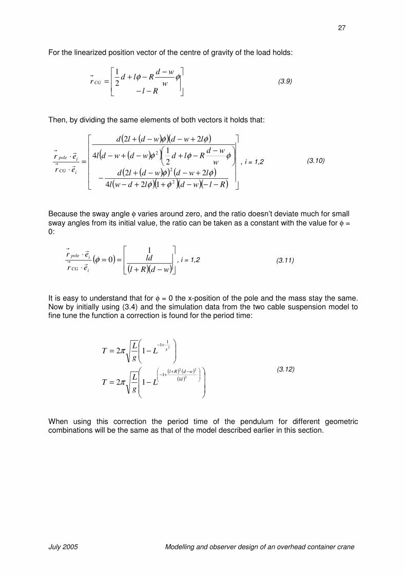
July 2005 Modelling and observer design of an overhead container crane
For the linearized position vector of the centre of gravity of the load holds:
−−
−−+
=Rl
w
wdRld
r CGφφ
2
1
(3.9)
Then, by dividing the same elements of both vectors it holds that:
( )( )( )
( )( )
( )( ) ( )( )( )( )( )
−−−++−
+−−+−
−−+−+−
+−−+
=⋅
⋅
Rlwdldwl
lwdwdld
w
wdRldwdwdl
lwdwdld
er
er
iCG
ipole
2
2
2
124
22
2
14
22
φφ
φφ
φφφ
φφ
r
r
, i = 1,2
(3.10)
Because the sway angle φ varies around zero, and the ratio doesn’t deviate much for small
sway angles from its initial value, the ratio can be taken as a constant with the value for φ = 0:
( )( )( )
−+==
⋅
⋅
wdRl
ld
er
er
iCG
ipole1
0φr
r
, i = 1,2
(3.11)
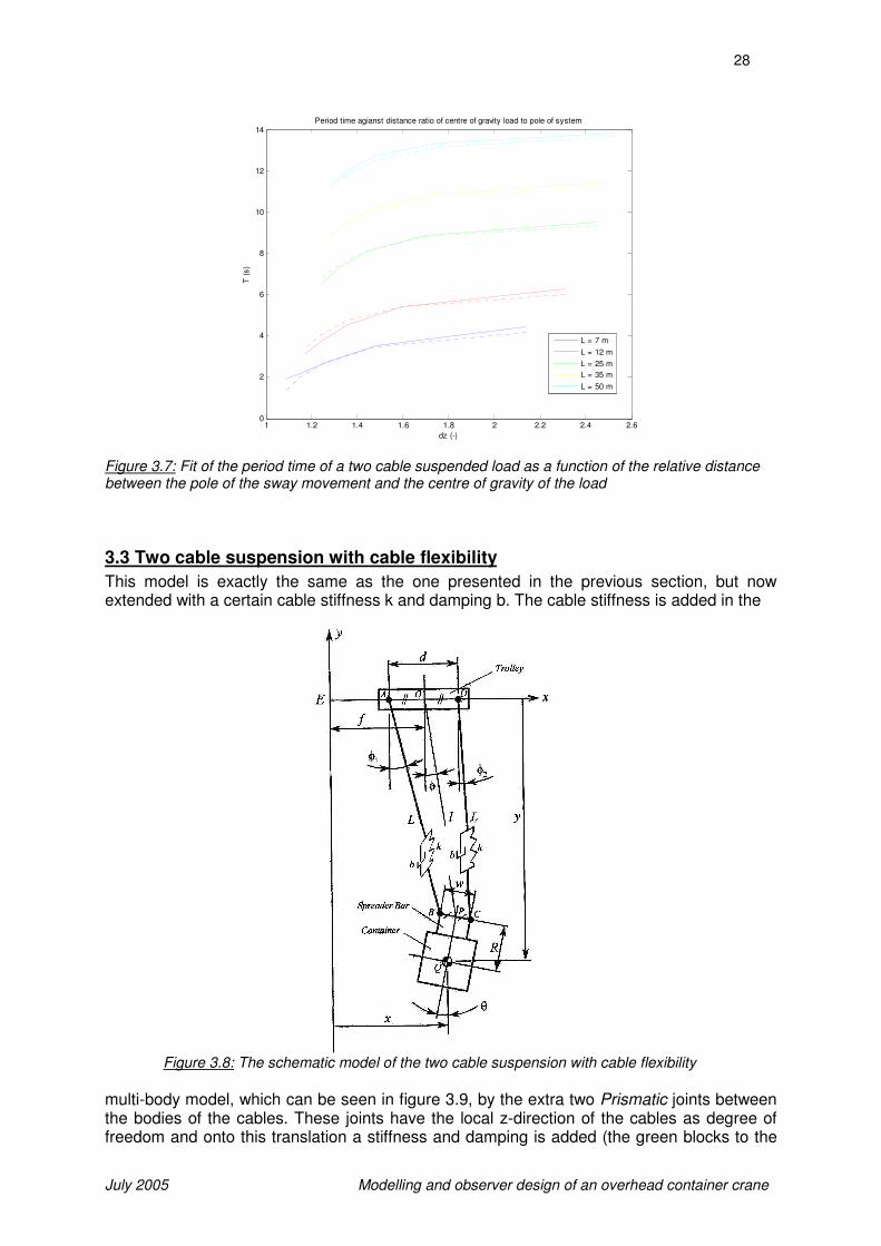
It is easy to understand that for φ = 0 the x-position of the pole and the mass stay the same. Now by initially using (3.4) and the simulation data from the two cable suspension model to fine tune the function a correction is found for the period time:
−=
+−2
11
12 xLg
LT π
( ) ( )( )
−=
−++−
2
22
1
12ld
wdRl
Lg
LT π
(3.12)
When using this correction the period time of the pendulum for different geometric combinations will be the same as that of the model described earlier in this section.
28
July 2005 Modelling and observer design of an overhead container crane
1 1.2 1.4 1.6 1.8 2 2.2 2.4 2.60
2
4
6
8
10
12
14Period time agianst distance ratio of centre of gravity load to pole of system
dz (-)
T (
s)
L = 7 m
L = 12 m
L = 25 m
L = 35 m
L = 50 m
Figure 3.7: Fit of the period time of a two cable suspended load as a function of the relative distance between the pole of the sway movement and the centre of gravity of the load
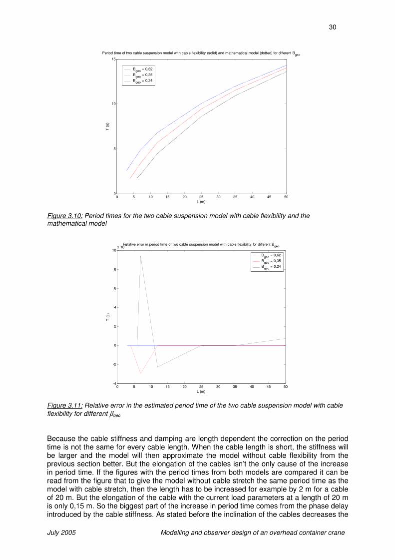
3.3 Two cable suspension with cable flexibility
This model is exactly the same as the one presented in the previous section, but now extended with a certain cable stiffness k and damping b. The cable stiffness is added in the
Figure 3.8: The schematic model of the two cable suspension with cable flexibility
multi-body model, which can be seen in figure 3.9, by the extra two Prismatic joints between the bodies of the cables. These joints have the local z-direction of the cables as degree of freedom and onto this translation a stiffness and damping is added (the green blocks to the

29
July 2005 Modelling and observer design of an overhead container crane
left and right of these joints), representing the cables as a parallel spring and damper. The extra blocks on the left side of the model, which are connected with the input of the cable lengths, contain the function to calculate the cable stiffness and damping which are cable-length dependent. The model has two extra outputs, the stretch of cable 1 and cable 2, which
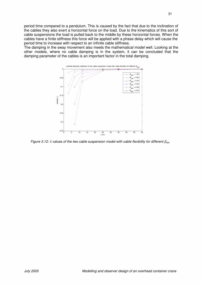
are also two extra states to describe the dynamics of the model. In figure 3.10 the simulated period times for this model are plotted together with that of the mathematical model. The period time is now estimated very accurately. As can be seen in figure 3.11 the maximum relative errors are of an order 10-3. Because these errors are so small it can be assumed they are caused by inaccurate reading of the figures and not by model errors. The period time has increased compared to the model without cable flexibility. Part of this can be directed back to the elongation of the cables due to the introduced finite cable stiffness. The cable stiffness and damping are:
L
kkcable
0= (3.13)
L
bbcable
0= (3.14)
6
Stretch of cable2 (m)
5
Stretch of cable 1 (m)
4
x(2) - Sway angle speed cable 1 (degs-1)
3
x(1) - Sway angle cable 1 (deg)
2
y(2) - Sway angle pendulum (deg)
1
y(1) - Horizontal posi tion trol ley (m)
CS
1
CS
2
CS
3
CS
4
CS
5
Trol ley
cable2_prop
To Workspace1
cable1_prop
To Workspace
In1Out1
Subsystem2
In1Out1
Subsystem1
BF
Revolute2b
B
F
Revolute2a
BF
Revolute1b
B
F
Revolute1a
BF
Prismatic5
BF
Prismatic4
B
F
Prismatic3
B
F
Prismatic2
B
F
Prismatic1
In1Out1
PD-controller
Env
Machine
Environment
CS
1
CS
2
CS
3
Load (headblock, spreader, container)
Joint Spring & Damper3Joint Spring & Damper
Joint Sensor3 Joint Sensor2
Joint Sensor1
Joint Actuator1 Joint Actuator
Initial trol ley condi tions
Initial sway condi tions
Ground
[trol ley_pv]Goto1
[spreader_pv]Goto
[spreader_pv]
From1
[trol ley_pv]
From
u(1)
Fcn2
f(u)
Fcn1
u(1)
Fcn
b02
Constant4
k02
Constant3
b01
Constant2
k01
Constant1
0
Constant
MATLAB
Function
Cable properties1
MATLAB
Function
Cable properties
CS
1C
S2
Cable 2c
CS
1C
S2
Cable 2b
CS
1C
S2
Cable 2a
L02Cable 2 ini tial length
CS
1C
S2
Cable 1c
CS
1C
S2
Cable 1b
CS
1C
S2
Cable 1aL01Cable 1 ini tial length
Body Sensor1
Body Sensor
Body Actuator
2
u(3) - Length of cables (m)
1
u(1) Position trolley
Figure 3.9: The multi-body model of the two cable suspension crane with cable flexibility
30
July 2005 Modelling and observer design of an overhead container crane
Because the cable stiffness and damping are length dependent the correction on the period time is not the same for every cable length. When the cable length is short, the stiffness will be larger and the model will then approximate the model without cable flexibility from the previous section better. But the elongation of the cables isn’t the only cause of the increase in period time. If the figures with the period times from both models are compared it can be read from the figure that to give the model without cable stretch the same period time as the model with cable stretch, then the length has to be increased for example by 2 m for a cable of 20 m. But the elongation of the cable with the current load parameters at a length of 20 m is only 0,15 m. So the biggest part of the increase in period time comes from the phase delay introduced by the cable stiffness. As stated before the inclination of the cables decreases the
0 5 10 15 20 25 30 35 40 45 500
5
10
15
Period time of two cable suspension model with cable flexibility (solid) and mathematical model (dotted) for different Bgeo
L (m)
T (
s)
Bgeo
= 0,62
Bgeo
= 0,35
Bgeo
= 0,24
Figure 3.10: Period times for the two cable suspension model with cable flexibility and the mathematical model
0 5 10 15 20 25 30 35 40 45 50-4
-2
0
2
4
6
8
10x 10
-3Relative error in period time of two cable suspension model with cable flexibility for different Bgeo
L (m)
T (
s)
Bgeo
= 0,62
Bgeo
= 0,35
Bgeo
= 0,24
Figure 3.11: Relative error in the estimated period time of the two cable suspension model with cable
flexibility for different βgeo
31
July 2005 Modelling and observer design of an overhead container crane
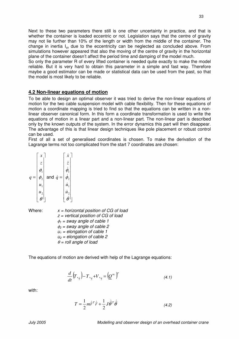
period time compared to a pendulum. This is caused by the fact that due to the inclination of the cables they also exert a horizontal force on the load. Due to the kinematics of this sort of cable suspensions the load is pulled back to the middle by these horizontal forces. When the cables have a finite stiffness this force will be applied with a phase delay which will cause the period time to increase with respect to an infinite cable stiffness. The damping in the sway movement also meets the mathematical model well. Looking at the other models, where no cable damping is in the system, it can be concluded that the damping parameter of the cables is an important factor in the total damping.
0 5 10 15 20 25 30 35 40 45 50-0.35
-0.3
-0.25
-0.2
-0.15
-0.1
-0.05
0
Lambda damping coefficient of two cable suspension model with cable flexibility for different Bgeo
L (m)
lam
bda (
-)
Bgeo
= 1,00
Bgeo
= 0,62
Bgeo
= 0,44
Bgeo
= 0,35
Bgeo
= 0,29
Bgeo
= 0,24
Figure 3.12: λ values of the two cable suspension model with cable flexibility for different βgeo

32
July 2005 Modelling and observer design of an overhead container crane
4. Application of the chosen model
4.1 Parameter sensitivity
In the two cable suspension model with cable flexibility some parameters are used which aren’t exactly known in reality. These parameters are the height of the centre of gravity of the load R (see figure 2.10) and the inertia of the load Iyy. For every container that is unloaded from a ship these two parameters are different and depend on the mass and placement of the cargo in the container. Because they are not known the model has to be robust in its estimation of the period time and damping for variation of these two parameters. For efficient loading of ships there are a couple of standard sizes for cargo containers. Common lengths for example are 20, 40 and 45 ft. The height normally varies between 8 and 10 ft, which is equal to 2,4 to 3,0 m. For R therefore a standard value of 1,5 m was chosen, because then the centre of gravity lies approximately in the middle of the container. For the variation of this parameter only lower centre of gravities are considered (so a larger R), because of the way containers are loaded. In figure 4.1 the relative difference in period time can be seen for R = 2,5 and R = 3,0 m. They are compared with the standard value R = 1,5 m. It can be seen that for parallel cables the period time becomes larger. This is easy to
5 10 15 20 25 30 35 40 45 50-0.15
-0.1
-0.05
0
0.05
0.1Sensitivity of parameter R with respect to period time (solid: R = 2.5 m, dotted: R = 3.0 m)
L (m)
(-)
Bgeo
= 1.00
Bgeo
= 0.44
Bgeo
= 0.29
Figure 4.1: The sensitivity of parameter R on the period time of the model
understand because of the increased pendulum length. For an inclination of the cables it makes less sense, but it can be concluded that the parameter R has some influence on the period time of the sway movement. From the same simulations it also appeared that the parameter affects the damping. Also the sensitivity for the inertia Iyy was tested, but variation of this parameter between 30000 and 60000 kgm2 (the standard value is 45000 kgm2) made a negligible difference in the period time and damping.
33
July 2005 Modelling and observer design of an overhead container crane
Next to these two parameters there still is one other uncertainty in practice, and that is whether the container is loaded eccentric or not. Legislation says that the centre of gravity may not lie further than 10% of the length or width from the middle of the container. The change in inertia Iyy due to the eccentricity can be neglected as concluded above. From simulations however appeared that also the moving of the centre of gravity in the horizontal plane of the container doesn’t affect the period time and damping of the model much. So only the parameter R of every lifted container is needed quite exactly to make the model reliable. But it is very hard to obtain this parameter in a simple and fast way. Therefore maybe a good estimator can be made or statistical data can be used from the past, so that the model is most likely to be reliable.
4.2 Non-linear equations of motion
To be able to design an optimal observer it was tried to derive the non-linear equations of motion for the two cable suspension model with cable flexibility. Then for these equations of motion a coordinate mapping is tried to find so that the equations can be written in a non-linear observer canonical form. In this form a coordinate transformation is used to write the equations of motion in a linear part and a non-linear part. The non-linear part is described only by the known outputs of the system. In the error dynamics this part will then disappear. The advantage of this is that linear design techniques like pole placement or robust control can be used. First of all a set of generalised coordinates is chosen. To make the derivation of the Lagrange terms not too complicated from the start 7 coordinates are chosen:
=
θ
φ
φ
2
1
2
1
u
u
z
x
q and
=
θ
φ
φ
&
&
&
&
&
&
&
&
2
1
2
1
u
u
z
x
q
Where: x = horizontal position of CG of load z = vertical position of CG of load
φ1 = sway angle of cable 1
φ2 = sway angle of cable 2 u1 = elongation of cable 1 u2 = elongation of cable 2
θ = roll angle of load The equations of motion are derived with help of the Lagrange equations:
( ) ( )Tnc
qqq QVTTdt
d=+− ,,, & (4.1)
with:
θθ&r&r&r&r TT
JrrmT2
1
2
1+= (4.2)

34
July 2005 Modelling and observer design of an overhead container crane
2
22
2
112
1
2
1ukukermgV z ++⋅= (4.3)
( ) ( ) ncT
q
ncT
q
ncFrFrQ 2211 ,, += (4.4)
and:
=
z
xr , [ ]θθ = ,
( ) ( )
( ) ( )
++
−+=
θθ
θθ
sin2
1cos
cos2
1sin
1
wRz
wRxr ,
( ) ( )
( ) ( )
−+
++=
θθ
θθ
sin2
1cos
cos2
1sin
2
wRz
wRxr
( )( )
−=
111
1111
cos
sin
φ
φ
ub
ubF
nc
&
&,
( )( )
=
222
2222
cos
sin
φ
φ
ub
ubF
nc
&
&
From the Lagrange equations the equations of motion can be written in the general form:
( ) ( ) ( )τqSqqHqqM =+ &&& , (4.5)
With: ( )
=
J
m
m
qM
000000
0000000
0000000
0000000
0000000
000000
000000
( )
( ) ( )( ) ( )
( ) ( ) ( ) ( ) ( ) ( )
( ) ( ) ( ) ( ) ( ) ( )
−−−
−−
+−−
+
−−
−
=
222222
111111
22
11
222111
222111
coscos2
1sinsinsin
2
1cos
coscos2
1sinsinsin
2
1cos
0
0
coscos
sinsin
,
φθθφθθ
φθθφθθ
φφ
φφ
ubwRubwR
ubwRubwR
uk
uk
ububmg
ubub
qqH
&&
&&
&&
&&
&
35
July 2005 Modelling and observer design of an overhead container crane
( )
=
0000000
0000000
0000000
0000000
0000000
0000000
0000000
qS ,
=
0
0
0
0
0
0
0
τ
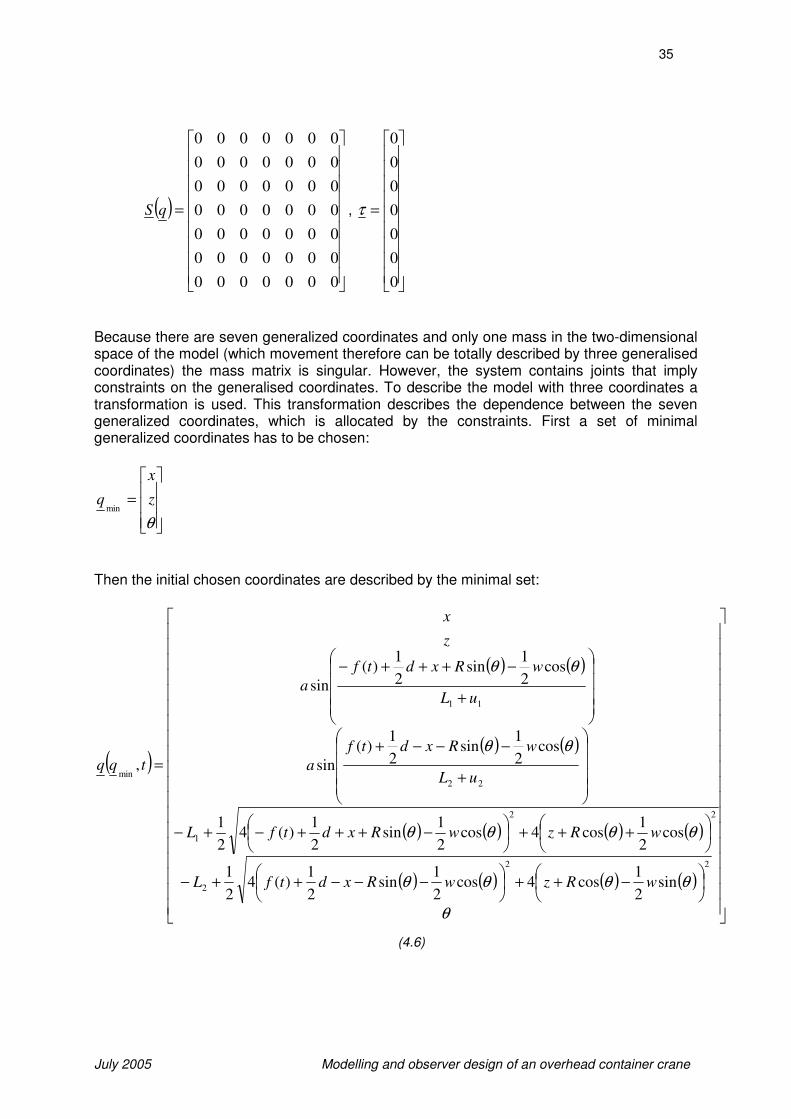
Because there are seven generalized coordinates and only one mass in the two-dimensional space of the model (which movement therefore can be totally described by three generalised coordinates) the mass matrix is singular. However, the system contains joints that imply constraints on the generalised coordinates. To describe the model with three coordinates a transformation is used. This transformation describes the dependence between the seven generalized coordinates, which is allocated by the constraints. First a set of minimal generalized coordinates has to be chosen:
=
θ
z
x
qmin
Then the initial chosen coordinates are described by the minimal set:
( )
( ) ( )
( ) ( )
( ) ( ) ( ) ( )
( ) ( ) ( ) ( )
−++
−−−++−
+++
−+++−+−
+
−−−+
+
−+++−
=
θ
θθθθ
θθθθ
θθ
θθ
22
2
22
1
22
11
min
sin2
1cos4cos
2
1sin
2
1)(4
2
1
cos2
1cos4cos
2
1sin
2
1)(4
2
1
cos2
1sin
2
1)(
sin
cos2
1sin
2
1)(
sin
,
wRzwRxdtfL
wRzwRxdtfL
uL
wRxdtf
a
uL
wRxdtf
a
z
x
tqq
(4.6)

36
July 2005 Modelling and observer design of an overhead container crane
From these equations the transformation matrices can be determined:
( )( )
min
min
min
,,
qd
tqqdtqT =
( ) ( )dt
tqqdtq
,,~ min
min=κ
( ) ( ) ( )tqqqtqqTtqq ,,~,,,,minminminminminminmin
&&&&&& κκ +=
(4.7)
which then leads to the new equations of motion:
τκ c
T
c
T
c
T
c
TSTMTHTqTMT =++
min&&
( ) ( )κτ c
T
c
T
c
T
c
TMTHTSTTMTq −−=
−1
min&&
(4.8)
where: ( ) ( )( )ttqqMtqM c ,,,minmin
=
( ) ( ) ( ) ( )( )ttqqtqTtqqHtqqH c ,,,,,,,minminminminminmin
κ+= &&
( ) ( )( )ttqqStqS c ,,,minmin
=
After applying this method however the equations of motion found for the model were so long and complex that they are practically unusable. This is a disadvantage that can be seen more often with multi-body models.
4.3 Linearization
Because the non-linear equations of motion can’t be used, another way of analysing this model has to be found. Therefore it was tried to linearize this model. This is done with help of the Linear Analyser in the Tools and Estimation Manager in Matlab/Simulink. This tool linearizes the non-linear equations of motion in a pre defined operation point after choosing the appropriate input- and output signals. The model can be linearized analytically block-by-block, or by numerical perturbation like frequency response measurements on a real system. As inputs the trolley position xtr and the hoist height dL are chosen. As output the sway angle
φ is chosen. The operation point can be set and generally an equilibrium point is chosen. This system reaches a steady-state situation when the sway- and roll angle of the load are zero, only the elongation of the cables is non-zero and depends on the length of the cables
and the geometry parameter βgeo. By simulation the operation points are determined for the
different combinations of cable lengths L and geometry parameter βgeo. The Linear Analyser automatically chooses the states of the system. Because the model contains a separate body for the trolley, the trolley position and velocity are also chosen as 2 states. But in this case it is assumed again that the position control of the trolley is perfect and therefore these two parameters are constraints of the system instead of degrees of freedom. And as could be seen in (2.33), when the trolley position is seen as a degree of freedom this has influence on the estimated period time of the model. To overcome this problem the mass of the trolley
37
July 2005 Modelling and observer design of an overhead container crane
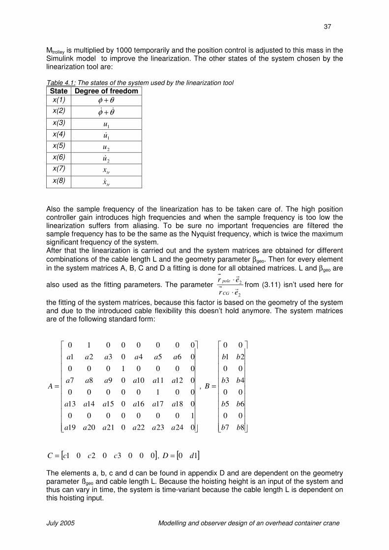
Mtrolley is multiplied by 1000 temporarily and the position control is adjusted to this mass in the Simulink model to improve the linearization. The other states of the system chosen by the linearization tool are: Table 4.1: The states of the system used by the linearization tool
State Degree of freedom x(1) θφ +
x(2) θφ && +
x(3) 1u
x(4) 1u&
x(5) 2u
x(6) 2u&
x(7) trx
x(8) trx&
Also the sample frequency of the linearization has to be taken care of. The high position controller gain introduces high frequencies and when the sample frequency is too low the linearization suffers from aliasing. To be sure no important frequencies are filtered the sample frequency has to be the same as the Nyquist frequency, which is twice the maximum significant frequency of the system. After that the linearization is carried out and the system matrices are obtained for different
combinations of the cable length L and the geometry parameter βgeo. Then for every element
in the system matrices A, B, C and D a fitting is done for all obtained matrices. L and βgeo are
also used as the fitting parameters. The parameter
2
2
er
er
CG
pole
r
r
⋅
⋅from (3.11) isn’t used here for
the fitting of the system matrices, because this factor is based on the geometry of the system and due to the introduced cable flexibility this doesn’t hold anymore. The system matrices are of the following standard form:
=
02423220212019
10000000
01817160151413
00100000
01211100987
00001000
06540321
00000010
aaaaaa
aaaaaa
aaaaaa
aaaaaa
A ,
=
87
00
65
00
43
00
21
00
bb
bb
bb
bb
B
[ ]00030201 cccC = , [ ]10 dD =
The elements a, b, c and d can be found in appendix D and are dependent on the geometry parameter ßgeo and cable length L. Because the hoisting height is an input of the system and thus can vary in time, the system is time-variant because the cable length L is dependent on this hoisting input.
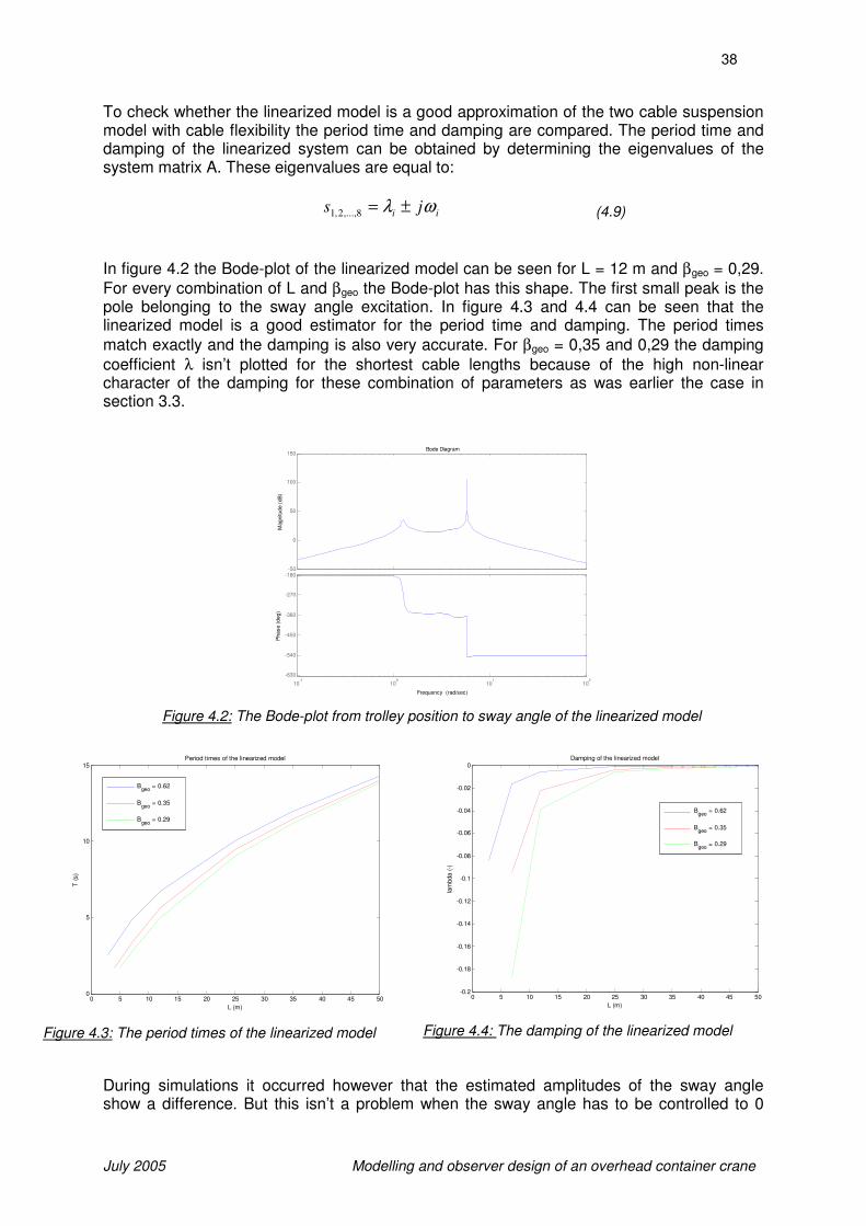
38
July 2005 Modelling and observer design of an overhead container crane
To check whether the linearized model is a good approximation of the two cable suspension model with cable flexibility the period time and damping are compared. The period time and damping of the linearized system can be obtained by determining the eigenvalues of the system matrix A. These eigenvalues are equal to:
ii js ωλ ±=8,...,2,1 (4.9)
In figure 4.2 the Bode-plot of the linearized model can be seen for L = 12 m and βgeo = 0,29.
For every combination of L and βgeo the Bode-plot has this shape. The first small peak is the pole belonging to the sway angle excitation. In figure 4.3 and 4.4 can be seen that the linearized model is a good estimator for the period time and damping. The period times
match exactly and the damping is also very accurate. For βgeo = 0,35 and 0,29 the damping
coefficient λ isn’t plotted for the shortest cable lengths because of the high non-linear character of the damping for these combination of parameters as was earlier the case in section 3.3.
During simulations it occurred however that the estimated amplitudes of the sway angle show a difference. But this isn’t a problem when the sway angle has to be controlled to 0
-50
0
50
100
150
Magnitu
de (
dB
)
10-1
100
101
102
-630
-540
-450
-360
-270
-180
Phase (
deg)
Bode Diagram
Frequency (rad/sec)
Figure 4.2: The Bode-plot from trolley position to sway angle of the linearized model
0 5 10 15 20 25 30 35 40 45 500
5
10
15Period times of the linearized model
L (m)
T (
s)
Bgeo
= 0.62
Bgeo
= 0.35
Bgeo
= 0.29
Figure 4.3: The period times of the linearized model
0 5 10 15 20 25 30 35 40 45 50-0.2
-0.18
-0.16
-0.14
-0.12
-0.1
-0.08
-0.06
-0.04
-0.02
0Damping of the linearized model
L (m)
lam
bda
(-)
Bgeo
= 0.62
Bgeo
= 0.35
Bgeo
= 0.29
Figure 4.4: The damping of the linearized model

39
July 2005 Modelling and observer design of an overhead container crane
degree, because when the period time matches that of the mathematical model the sway angle will be 0 degree at the same moment in time. Note that it has to be taken into account that this linearization isn’t reliable for variation of the
other parameters than L and βgeo. A new linearization has to be made when varying those parameters.
4.4 Observer design
To be able to synchronise this model with the real crane an observer has to be designed. First it is checked whether the model is observable anyway. A system is observable when: For the linearized model n = 8 and this is also the rank of the observer matrix so from (4.11) follows that the linearized model is observable. When the real crane, with which the observer has to be synchronized, is represented as the linear model the error dynamics can be formulated:
( )ePCAe −=& (4.12)
where P is the feedback gain matrix. By pole placement a stabilizing observer gain can be determined now. It has to be taken care of however that the stability and performance of the feedback are good for every combination
of L and βgeo, except for 105 <≤ L m when the sway angle isn’t measured. The observer also has to be robust for small differences and unmodelled dynamics of the linear model compared to the real system. Because there is only one output fed back, the desired poles of the error dynamics may not have a multiplicity more than one, which means all chosen poles must have a different location on the root locus diagram. For the design of the observer gains the system matrices for a cable length of L = 50 m are chosen, because in this configuration the system has the least damping of itself. The poles of (4.12) are chosen as the poles of the system, but from the real part 10 is subtracted. This leads to the following observer gains:
P = [8552 –4743 2226 4766 10339 -770 -91 -636] The sway controller is always fed from the model and not directly from the measurement device. So also when the camera is able to measure the sway angle, the angle that is fed back comes from the synchronized model. This means that not only when the camera isn’t measuring the model produces the sway angle for the controller, but also when the camera is running. Therefore, when switching back from model stand-alone running to synchronization, it has to be watched that the synchronization effort isn’t too large on the model, because then the sway angle will show very rapid changes. And when that is fed back the actuators of the trolley positioning will saturate. Taking this into account, and the wide range of stability asked (as well due to the time-variant system matrix as due to the model uncertainty), it could also be considered to use robust control design techniques to determine the most optimal synchronization feedback.
4.5 Exporting Simulink model
Another possibility is that the observer is already designed in the Simmechanics model. By adding an actuator to the pivot point of one of the hoist cables the sway angle can be synchronized with the measured sway angle from the crane by a feedback controller. With the current possibilities of Matlab it is possible to export the model in C-code. Then by defining the right inputs and outputs and maybe some modifications to make it compatible with the hardware, this code can be used in the HIPAC software. This way of implanting
( ) nCACACACrankTn =−12
K (4.11)

40
July 2005 Modelling and observer design of an overhead container crane
models is more and more used in various eminent industries. For example in the automotive industry control units of cars are programmed with Matlab/Simulink. Very complex models and control strategies designed in Simulink can easily be programmed into existing software. Because of the block structure of Simulink it is easy to keep a clear vision on complex models and it is also easy to make changes. The only disadvantage of not analyzing the exact equations of motion is that the physical understanding of the system is less, but for complex equations that just isn’t always a realistic possibility.

41
July 2005 Modelling and observer design of an overhead container crane
5. Conclusions and recommendations
5.1 Conclusions
To be able to draw the right and valid conclusions one first has to question the reliability of the mathematical model disposed by Siemens, with which all other models are compared. From experience of the commissioning engineers of Siemens however this model can be assumed as a good and reliable representation of a real overhead container crane. In chapter 2 it was tried to adjust the current Siemens model. The two major problems of this model are that it doesn’t correct the period time and damping for different cable inclinations,
described with the parameter βgeo. Therefore two adjustments are suggested that account for this inclination by correcting the period time. The performance of the model becomes better for the range of geometry parameters, but the corrections aren’t perfect. Also a semi-empirical correction is suggested, coming from the momentary pole of the cable suspension, but this correction also doesn’t fit the period time exactly. Using the nominal test trajectory in simulation all three corrections perform approximately the same. Because of the periodic behaviour of the sway angle the errors made in the estimation of this angle have the same amplitude. Only the process will be different. A correction for the damping of the sway angle couldn’t be found by physical reasoning. With empirical ways the period time and damping can be fitted exactly by using measurement data of a real crane, but this method is only reliable for one crane and next to that the measurements are time consuming and not easy to do very accurate. Finally, also a model is treated where the trolley position and the cable length are degrees of freedom. By doing this the influence of the controllers of these motions on the pendulum period time can be simulated. Because this is a complete different (non-linear) model also an observer is designed for this model. The major cause of the still existing difference in the real- and estimated period time and damping is the cable flexibility and the corresponding dynamic behaviour. In chapter 3 the conclusion is already drawn that this cable flexibility is an important factor in the period time and damping of the sway movement. This could be seen in the difference of performance compared to the mathematical model of both two cable suspended models, respectively without and with cable flexibility. The model with cable flexibility fits the period time and damping almost exactly. However, mainly this introduction of the two extra states u1 and u2, the elongation of both hoist cables, makes the equations of motion very complex. These equations of motion are needed for implementation and observer design. Because of the complexity of the non-linear equations the model is linearized to obtain a state-space representation. For this model an observer is designed.
5.2 Recommendations
The first thing that can be recommended is that all proposed adjustments are tested in practice. Although the mathematical model is reliable, simulation never matches reality exactly. All improvements have to be programmed in C-code so they can be used in the HIPAC software on the model in Erlangen (see appendix E). Next to that it can be useful to build in tuning parameters, so for small differences between parameters in reality the models can be tuned case by case.

42
July 2005 Modelling and observer design of an overhead container crane
Still the best solution seems to be the exporting of the total multi-body two cable suspension model with cable flexibility. As described in section 4.5 this is a very strong capability of Matlab and is therefore very often used in all sorts of industries and applications nowadays. The practical implementation and compatibility with the hardware has to tested extensively so the necessary adjustments can be made. Also, with some more test results and practical experience the model can be extended even more.
43
July 2005 Modelling and observer design of an overhead container crane
Bibliography
[1] Nader A. Nayfeh (2002), Adaption of Delayed Position Feedback to the Reduction of Sway of Container Cranes, Blacksburg, Virginia
[2] Axel Buch (1999), Optimale Bewegungssteuerung von schwingungsfähigen mechatronischen Systemen met zwei Freiheitsgraden am Beispiel eines Krans mit pendelnder Last und elastischer Mechanik, Magdeburg
[3] Yong-Seok Kim, Keum-Shik Hong, Seung-Ki Sul (2004), “Anti-Sway Control of
Container Cranes: Inclinometer, Observer, and State Feedback”, in International Journal of Control, Automation and Systems, vol. 2, no. 4, pp. 435-449, December 2004
[4] R. van der Wekken (1996), Automatisering van de 2000-12 Jumbo Container Crane –
Dynamica van de spreader in een container kadekraan, Delft [5] Kyung-Tae Hong, Chang-Do Huh, Keum-Shik Hong (2003), “Command Shaping
Control for Limiting the Transient Sway Angle of Crane Systems”, in International Journal of Control, Automation, and Systems, vol. 1, no. 1, March 2003
[6] Keum-Shik Hong, Bae-Jeong Park, Man-Hyung Lee (2000), “Two-Stage Control for
Container Cranes”, in JSME International Journal, Series C, vol. 43, no. 2, 2000 [7] Bram de Kraker, Dick H. van Campen (2001), Mechanical Vibrations, Eindhoven [8] Nathan van de Wouw (2003), Multibody Dynamics, Eindhoven

44
July 2005 Modelling and observer design of an overhead container crane
List of symbols
βgeo geometry parameter (-)
d width of trolley (m) w width of spreader (m) R distance of spreader to centre of gravity of load (m) k cable stiffness (kNm-1) b cable damping (kNsm-1) L cable length (m) l pendulum length (m)
φ sway angle pendulum (deg)
φ1 sway angle cable 1 (deg)
φ2 sway angle cable 2 (deg)
x trolley position (m)
ωn natural frequency (rads-1)
T period time (s)
λ real part of pole (rads)
ξ dimensionless damping factor (-)
dL lifting height (m)

45
July 2005 Modelling and observer design of an overhead container crane
Appendix A
Simulated period times and damping coefficients of the different models
T (s) model 4
φφφφ= 1 deg φφφφ = 2 deg φφφφ = 5 deg φφφφ = 10 deg φφφφ = 20 deg
L = 3 m 2,32 2,32 2,32 2,32 2,32 L = 7 m 4,45 4,45 4,45 4,45 4,42 L = 12 m 6,27 6,27 6,27 6,27 6,25 L = 25 m 9,55 9,55 9,55 9,56 9,57 L = 35 m 11,46 11,46 11,46 11,47 11,50 L = 50 m 13,85 13,85 13,85 13,86 13,91
T (s) model 5
φφφφ= 1 deg φφφφ = 2 deg φφφφ = 5 deg φφφφ = 10 deg φφφφ = 20 deg
L = 3 m 2,57 2,57 2,58 2,58 2,59 L = 7 m 4,88 4,88 4,89 4,89 4,93 L = 12 m 6,76 6,76 6,77 6,78 6,83 L = 25 m 10,05 10,05 10,06 10,08 10,15 L = 35 m 11,95 11,95 11,96 11,98 12,05 L = 50 m 14,31 14,31 14,32 14,33 14,43
T (s) mathematical
model
φφφφ= 1 deg φφφφ = 2 deg φφφφ = 5 deg φφφφ = 10 deg φφφφ = 20 deg
L = 3 m 2,57 2,57 2,58 2,57 3,29*
L = 7 m 4,88 4,88 4,88 4,88 5,21*
L = 12 m 6,76 6,76 6,76 6,78 6,93 L = 25 m 10,05 10,05 10,06 10,08 10,15 L = 35 m 11,95 11,95 11,95 11,97 12,06 L = 50 m 14,31 14,31 14,32 14,34 14,43
*Italic numbers couldn’t be measured properly
T (s) model 4
ββββgeo = 1,00 [-]
ββββgeo = 0,62 [-]
ββββgeo = 0,44 [-]
ββββgeo = 0,35 [-]
ββββgeo = 0,29 [-]
ββββgeo = 0,24 [-]
L = 3 m 3,48 2,32 1,61 1,67*
1,70*
1,74*
L = 7 m 5,31 4,45 3,49 2,69 2,17 1,88 L = 12 m 6,96 6,27 5,42 4,55 3,78 3,16 L = 25 m 10,03 9,55 8,89 8,12 7,32 6,55 L = 35 m 11,87 11,46 10,88 10,19 9,44 8,67 L = 50 m 14,19 13,85 13,35 12,75 12,06 11,33
*Italic numbers have adjusted cable length, because 3 m was too short. The cable lengths
are respectively 4 m for βgeo = 0,35, 5 m for βgeo = 0,29 and 6 m for βgeo = 0,24
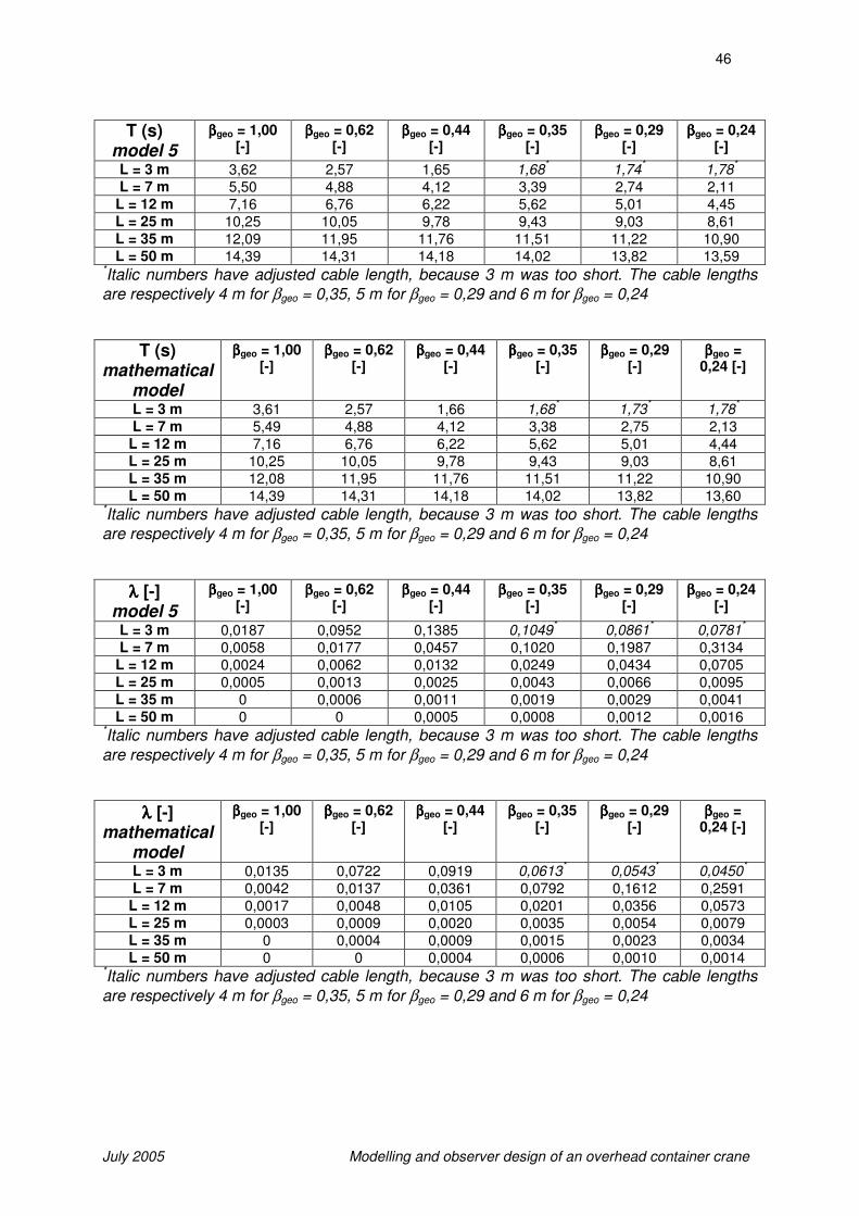
46
July 2005 Modelling and observer design of an overhead container crane
T (s) model 5
ββββgeo = 1,00 [-]
ββββgeo = 0,62 [-]
ββββgeo = 0,44 [-]
ββββgeo = 0,35 [-]
ββββgeo = 0,29 [-]
ββββgeo = 0,24 [-]
L = 3 m 3,62 2,57 1,65 1,68*
1,74*
1,78*
L = 7 m 5,50 4,88 4,12 3,39 2,74 2,11 L = 12 m 7,16 6,76 6,22 5,62 5,01 4,45 L = 25 m 10,25 10,05 9,78 9,43 9,03 8,61 L = 35 m 12,09 11,95 11,76 11,51 11,22 10,90 L = 50 m 14,39 14,31 14,18 14,02 13,82 13,59
*Italic numbers have adjusted cable length, because 3 m was too short. The cable lengths
are respectively 4 m for βgeo = 0,35, 5 m for βgeo = 0,29 and 6 m for βgeo = 0,24
T (s) mathematical
model
ββββgeo = 1,00 [-]
ββββgeo = 0,62 [-]
ββββgeo = 0,44 [-]
ββββgeo = 0,35 [-]
ββββgeo = 0,29 [-]
ββββgeo = 0,24 [-]
L = 3 m 3,61 2,57 1,66 1,68*
1,73*
1,78*
L = 7 m 5,49 4,88 4,12 3,38 2,75 2,13 L = 12 m 7,16 6,76 6,22 5,62 5,01 4,44 L = 25 m 10,25 10,05 9,78 9,43 9,03 8,61 L = 35 m 12,08 11,95 11,76 11,51 11,22 10,90 L = 50 m 14,39 14,31 14,18 14,02 13,82 13,60
*Italic numbers have adjusted cable length, because 3 m was too short. The cable lengths
are respectively 4 m for βgeo = 0,35, 5 m for βgeo = 0,29 and 6 m for βgeo = 0,24
λλλλ [-] model 5
ββββgeo = 1,00 [-]
ββββgeo = 0,62 [-]
ββββgeo = 0,44 [-]
ββββgeo = 0,35 [-]
ββββgeo = 0,29 [-]
ββββgeo = 0,24 [-]
L = 3 m 0,0187 0,0952 0,1385 0,1049*
0,0861*
0,0781*
L = 7 m 0,0058 0,0177 0,0457 0,1020 0,1987 0,3134 L = 12 m 0,0024 0,0062 0,0132 0,0249 0,0434 0,0705 L = 25 m 0,0005 0,0013 0,0025 0,0043 0,0066 0,0095 L = 35 m 0 0,0006 0,0011 0,0019 0,0029 0,0041 L = 50 m 0 0 0,0005 0,0008 0,0012 0,0016
*Italic numbers have adjusted cable length, because 3 m was too short. The cable lengths
are respectively 4 m for βgeo = 0,35, 5 m for βgeo = 0,29 and 6 m for βgeo = 0,24
λλλλ [-] mathematical
model
ββββgeo = 1,00 [-]
ββββgeo = 0,62 [-]
ββββgeo = 0,44 [-]
ββββgeo = 0,35 [-]
ββββgeo = 0,29 [-]
ββββgeo = 0,24 [-]
L = 3 m 0,0135 0,0722 0,0919 0,0613*
0,0543*
0,0450*
L = 7 m 0,0042 0,0137 0,0361 0,0792 0,1612 0,2591 L = 12 m 0,0017 0,0048 0,0105 0,0201 0,0356 0,0573 L = 25 m 0,0003 0,0009 0,0020 0,0035 0,0054 0,0079 L = 35 m 0 0,0004 0,0009 0,0015 0,0023 0,0034 L = 50 m 0 0 0,0004 0,0006 0,0010 0,0014
*Italic numbers have adjusted cable length, because 3 m was too short. The cable lengths
are respectively 4 m for βgeo = 0,35, 5 m for βgeo = 0,29 and 6 m for βgeo = 0,24

47
July 2005 Modelling and observer design of an overhead container crane
Appendix B In figure 2.17 can be seen that the lines have a hyperbolic shape. With this information the following function is obtained by using the least squares method:
0 5 10 15 20 25 30 35 40 45 50-0.35
-0.3
-0.25
-0.2
-0.15
-0.1
-0.05
0Mathematical model lambda (solid) and fit of lambda (dotted)
L (m)
(-)
Bgeo
= 1,00
Bgeo
= 0,62
Bgeo
= 0,44
Bgeo
= 0,35
Bgeo
= 0,29
Bgeo
= 0,24
As can be seen this function is only dependent on βgeo and L. The other parameters, the load mass M, the load inertia J and the cable properties aren’t taken into account here. So for other combinations of these parameters the fitting has to be reconsidered.
( ) ( ) ( ) ( )77.055.03
2245.126762.64389.10141.00017.0
LLLLgeogeogeogeo ββββ
λ ++−+−=
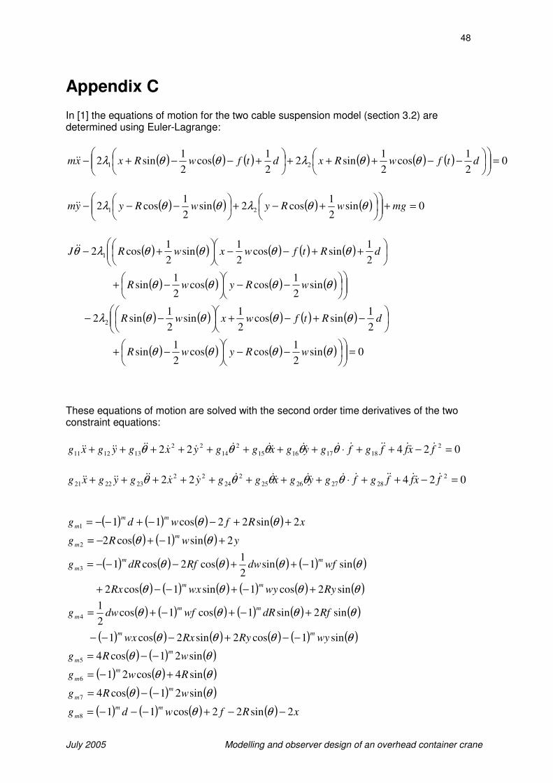
48
July 2005 Modelling and observer design of an overhead container crane
Appendix C
In [1] the equations of motion for the two cable suspension model (section 3.2) are determined using Euler-Lagrange:
( ) ( ) ( ) ( ) ( ) ( ) 02
1cos
2
1sin2
2
1cos
2
1sin2 21 =
−−+++
+−−+− dtfwRxdtfwRxxm θθλθθλ&&
( ) ( ) ( ) ( ) 0sin2
1cos2sin
2
1cos2 21 =+
+−+
−−− mgwRywRyym θθλθθλ&&
( ) ( ) ( ) ( ) ( )
++−−
+− dRtfwxwRJ
2
1sincos
2
1sin
2
1cos2 1 θθθθλθ&&
( ) ( ) ( ) ( )
−−
−+ θθθθ sin
2
1coscos
2
1sin wRywR
( ) ( ) ( ) ( ) ( )
−+−+
−− dRtfwxwR
2
1sincos
2
1sin
2
1sin2 2 θθθθλ
( ) ( ) ( ) ( ) 0sin2
1coscos
2
1sin =
−−
−+ θθθθ wRywR
These equations of motion are solved with the second order time derivatives of the two constraint equations:
024222
18171615
2
14
22
131211 =−++⋅++++++++ fxffgfgygxggyxgygxg &&&&&&&&&&&&&&&&&&&& θθθθθ
024222
28272625
2
24
22
232221 =−++⋅++++++++ fxffgfgygxggyxgygxg &&&&&&&&&&&&&&&&&&&& θθθθθ
( ) ( ) ( ) ( ) xRfwdgmm
m 2sin22cos111 ++−−+−−= θθ
( ) ( ) ( ) ywRgm
m 2sin1cos22 +−+−= θθ
( ) ( ) ( ) ( ) ( ) ( )
( ) ( ) ( ) ( ) ( ) ( )θθθθ
θθθθ
sin2cos1sin1cos2
sin1sin2
1cos2cos13
RywywxRx
wfdwRfdRg
mm
mm
m
+−+−−+
−++−−−=
( ) ( ) ( ) ( ) ( ) ( )
( ) ( ) ( ) ( ) ( ) ( )θθθθ
θθθθ
sin1cos2sin2cos1
sin2sin1cos1cos2
14
wyRyRxwx
RfdRwfdwg
mm
mm
m
−−+−−−
+−+−+=
( ) ( ) ( )θθ sin21cos45 wRgm
m −−=
( ) ( ) ( )θθ sin4cos216 Rwgm
m +−=
( ) ( ) ( )θθ sin21cos47 wRgm
m −−=
( ) ( ) ( ) ( ) xRfwdgmm
m 2sin22cos118 −−+−−−= θθ
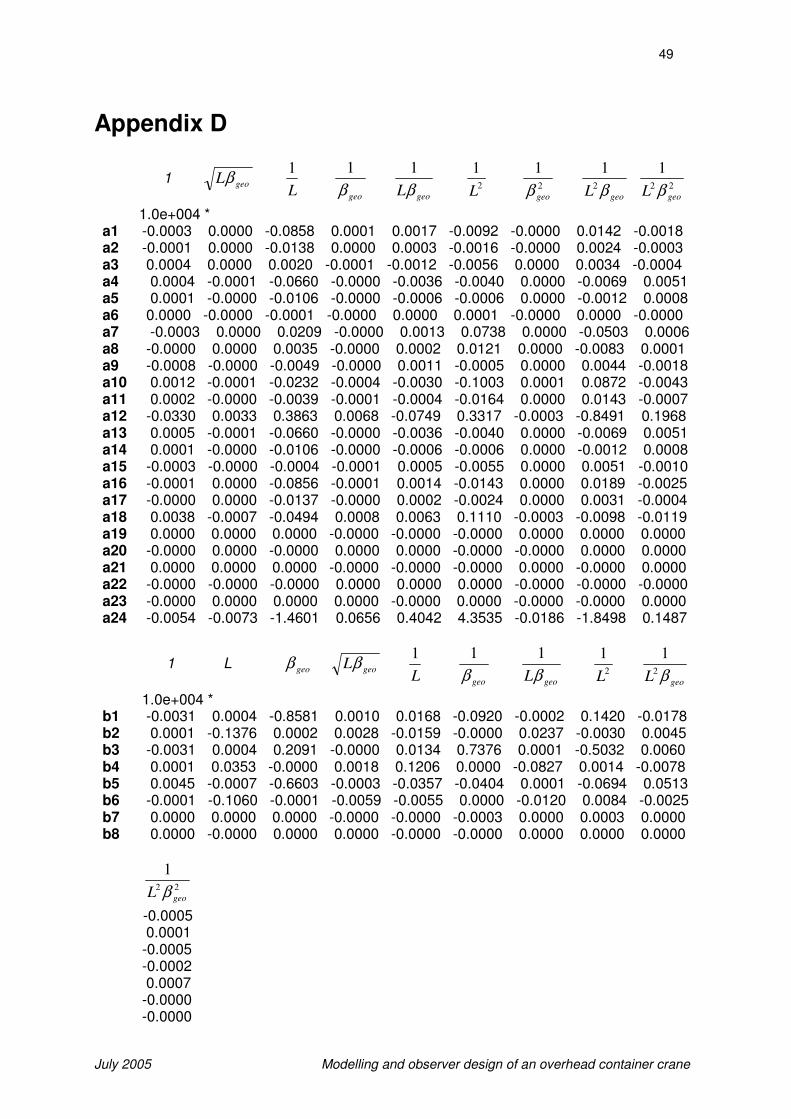
49
July 2005 Modelling and observer design of an overhead container crane
Appendix D
1 geoLβ L
1
geoβ
1
geoLβ
1
2
1
L
2
1
geoβ
geoL β2
1
22
1
geoL β
1.0e+004 * a1 -0.0003 0.0000 -0.0858 0.0001 0.0017 -0.0092 -0.0000 0.0142 -0.0018 a2 -0.0001 0.0000 -0.0138 0.0000 0.0003 -0.0016 -0.0000 0.0024 -0.0003 a3 0.0004 0.0000 0.0020 -0.0001 -0.0012 -0.0056 0.0000 0.0034 -0.0004 a4 0.0004 -0.0001 -0.0660 -0.0000 -0.0036 -0.0040 0.0000 -0.0069 0.0051 a5 0.0001 -0.0000 -0.0106 -0.0000 -0.0006 -0.0006 0.0000 -0.0012 0.0008 a6 0.0000 -0.0000 -0.0001 -0.0000 0.0000 0.0001 -0.0000 0.0000 -0.0000 a7 -0.0003 0.0000 0.0209 -0.0000 0.0013 0.0738 0.0000 -0.0503 0.0006 a8 -0.0000 0.0000 0.0035 -0.0000 0.0002 0.0121 0.0000 -0.0083 0.0001 a9 -0.0008 -0.0000 -0.0049 -0.0000 0.0011 -0.0005 0.0000 0.0044 -0.0018 a10 0.0012 -0.0001 -0.0232 -0.0004 -0.0030 -0.1003 0.0001 0.0872 -0.0043 a11 0.0002 -0.0000 -0.0039 -0.0001 -0.0004 -0.0164 0.0000 0.0143 -0.0007 a12 -0.0330 0.0033 0.3863 0.0068 -0.0749 0.3317 -0.0003 -0.8491 0.1968 a13 0.0005 -0.0001 -0.0660 -0.0000 -0.0036 -0.0040 0.0000 -0.0069 0.0051 a14 0.0001 -0.0000 -0.0106 -0.0000 -0.0006 -0.0006 0.0000 -0.0012 0.0008 a15 -0.0003 -0.0000 -0.0004 -0.0001 0.0005 -0.0055 0.0000 0.0051 -0.0010 a16 -0.0001 0.0000 -0.0856 -0.0001 0.0014 -0.0143 0.0000 0.0189 -0.0025 a17 -0.0000 0.0000 -0.0137 -0.0000 0.0002 -0.0024 0.0000 0.0031 -0.0004 a18 0.0038 -0.0007 -0.0494 0.0008 0.0063 0.1110 -0.0003 -0.0098 -0.0119 a19 0.0000 0.0000 0.0000 -0.0000 -0.0000 -0.0000 0.0000 0.0000 0.0000 a20 -0.0000 0.0000 -0.0000 0.0000 0.0000 -0.0000 -0.0000 0.0000 0.0000 a21 0.0000 0.0000 0.0000 -0.0000 -0.0000 -0.0000 0.0000 -0.0000 0.0000 a22 -0.0000 -0.0000 -0.0000 0.0000 0.0000 0.0000 -0.0000 -0.0000 -0.0000 a23 -0.0000 0.0000 0.0000 0.0000 -0.0000 0.0000 -0.0000 -0.0000 0.0000 a24 -0.0054 -0.0073 -1.4601 0.0656 0.4042 4.3535 -0.0186 -1.8498 0.1487
1 L geoβ geoLβ L
1
geoβ
1
geoLβ
1
2
1
L
geoL β2
1
1.0e+004 * b1 -0.0031 0.0004 -0.8581 0.0010 0.0168 -0.0920 -0.0002 0.1420 -0.0178 b2 0.0001 -0.1376 0.0002 0.0028 -0.0159 -0.0000 0.0237 -0.0030 0.0045 b3 -0.0031 0.0004 0.2091 -0.0000 0.0134 0.7376 0.0001 -0.5032 0.0060 b4 0.0001 0.0353 -0.0000 0.0018 0.1206 0.0000 -0.0827 0.0014 -0.0078 b5 0.0045 -0.0007 -0.6603 -0.0003 -0.0357 -0.0404 0.0001 -0.0694 0.0513 b6 -0.0001 -0.1060 -0.0001 -0.0059 -0.0055 0.0000 -0.0120 0.0084 -0.0025 b7 0.0000 0.0000 0.0000 -0.0000 -0.0000 -0.0003 0.0000 0.0003 0.0000 b8 0.0000 -0.0000 0.0000 0.0000 -0.0000 -0.0000 0.0000 0.0000 0.0000
22
1
geoL β
-0.0005 0.0001 -0.0005 -0.0002 0.0007 -0.0000 -0.0000
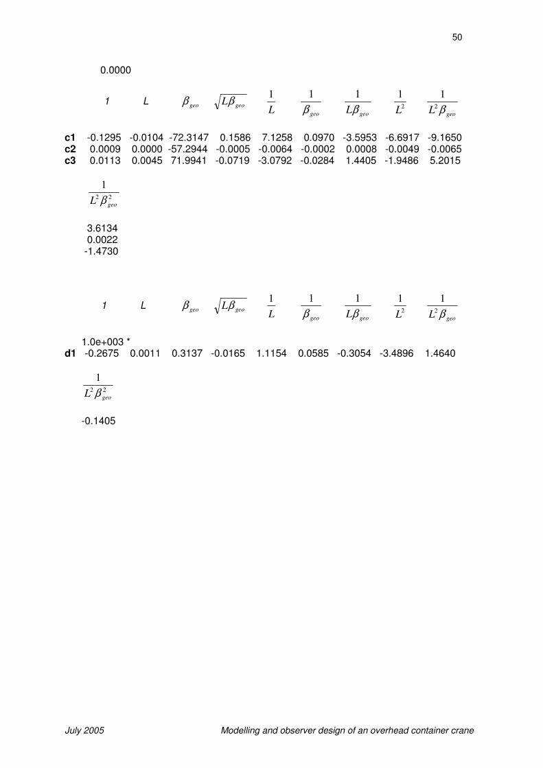
50
July 2005 Modelling and observer design of an overhead container crane
0.0000
1 L geoβ geoLβ L
1
geoβ
1
geoLβ
1
2
1
L
geoL β2
1
c1 -0.1295 -0.0104 -72.3147 0.1586 7.1258 0.0970 -3.5953 -6.6917 -9.1650 c2 0.0009 0.0000 -57.2944 -0.0005 -0.0064 -0.0002 0.0008 -0.0049 -0.0065 c3 0.0113 0.0045 71.9941 -0.0719 -3.0792 -0.0284 1.4405 -1.9486 5.2015
22
1
geoL β
3.6134 0.0022 -1.4730
1 L geoβ geoLβ L
1
geoβ
1
geoLβ
1
2
1
L
geoL β2
1
1.0e+003 * d1 -0.2675 0.0011 0.3137 -0.0165 1.1154 0.0585 -0.3054 -3.4896 1.4640
22
1
geoL β
-0.1405

51
July 2005 Modelling and observer design of an overhead container crane
Appendix E
![SEUSS: Skip Redundant Paths to Make Serverless Fast€¦ · Container in a MicroVM 450 1 to 7 s Linux v4.15; Docker v18.09; [Xeon 2.20 GHz; 88GB] less overhead more overhead less](https://img.pdfslide.net/doc/110x75/60299fb8113fa101cc59f608/seuss-skip-redundant-paths-to-make-serverless-fast-container-in-a-microvm-450-1.jpg)