Modelling climate change under no-policy and policy emissions pathways

Organisation for Economic Co-operation and Development 2003 Organisation de Coopération et de Développement Economiques

ENV/EPOC/GSP(2003)7/FINAL

WORKING PARTY ON GLOBAL AND STRUCTURAL POLICIES

OECD Workshop on the Benefits of Climate Policy: Improving Information for Policy Makers

Modelling climate change under no-policy and policy

emissions pathways

by

Tom M. L. Wigley


2

Copyright OECD, 2003

Application for permission to reproduce or translate all or part of this material should be addressed to the Head of Publications Services, OECD, 2 rue André Pascal, 75775 Paris, Cedex 16, France


3

FOREWORD

This paper was prepared for an OECD Workshop on the Benefits of Climate Policy: Improving Information for Policy Makers, held 12-13 December 2002. The aim of the Workshop and the underlying Project is to outline a conceptual framework to estimate the benefits of climate change policies, and to help organise information on this topic for policy makers. The Workshop covered both adaptation and mitigation policies, and related to different spatial and temporal scales for decision-making. However, particular emphasis was placed on understanding global benefits at different levels of mitigation -- in other words, on the incremental benefit of going from one level of climate change to another. Participants were also asked to identify gaps in existing information and to recommend areas for improvement, including topics requiring further policy-related research and testing. The Workshop brought representatives from governments together with researchers from a range of disciplines to address these issues. Further background on the workshop, its agenda and participants, can be found on the internet at: www.oecd.org/env/cc

The overall Project is overseen by the OECD Working Party on Global and Structural Policy (Environment Policy Committee). The Secretariat would like to thank the governments of Canada, Germany and the United States for providing extra-budgetary financial support for the work.

This paper is issued as an authored “working paper” -- one of a series emerging from the Project. The ideas expressed in the paper are those of the author alone and do not necessarily represent the views of the OECD or its Member Countries.

As a working paper, this document has received only limited peer review. Some authors will be further refining their papers, either to eventually appear in the peer-reviewed academic literature, or to become part of a forthcoming OECD publication on this Project. The objective of placing these papers on the internet at this stage is to widely disseminate the ideas contained in them, with a view toward facilitating the review process.

Any comments on the paper may be sent directly to the author(s) at:

Tom M. L. Wigley National Center for Atmospheric Research, Boulder, CO, USA Email: [email protected]

Comments or suggestions concerning the broader OECD Project may be sent to the Project Manager:

Jan Corfee Morlot at: [email protected]

ACKNOWLEDGMENTS

This paper was commissioned by the OECD. Ben Santer (PCMDI, LLNL) prepared the maps presented in Figure 10. The National Center for Atmospheric Research is supported by the National Science Foundation.


4

TABLE OF CONTENTS

FOREWORD.................................................................................................................................................. 3

EXECUTIVE SUMMARY ............................................................................................................................ 5

1. INTRODUCTION ............................................................................................................................... 6

2. FUTURE EMISSIONS........................................................................................................................ 7

3. FUTURE CHANGES IN GLOBAL-MEAN TEMPERATURE....................................................... 14

4. SOURCES OF UNCERTAINTY IN GLOBAL-MEAN TEMPERATURE PROJECTIONS ......... 18

6. SPATIAL PATTERNS OF CLIMATE CHANGE ........................................................................... 23

7. TEMPERATURE PROJECTION UNDER CO2 STABILIZATION................................................ 28

8. CONCLUSIONS ............................................................................................................................... 30

9. REFERENCES .................................................................................................................................. 31

Tables

Table 1. Sources and magnitudes of uncertainties.............................................................................. 20 Figures

Figure 1. Extremes of fossil CO2 emissions from the full set of 35 complete SRES scenarios ............ 8 Figure 2. CO2 concentration projections corresponding to Figure 1 ..................................................... 9 Figure 3. Updated versions of the WRE concentration stabilization profiles for CO2........................ 12 Figure 4. Total CO2 emissions (fossil plus land-use change) for the WRE and overshoot

concentration profiles given in Figure 3 ............................................................................... 13 Figure 5. Global-mean temperature projections for the IPCC SRES emissions scenarios .................. 16 Figure 6. No-climate-policy probabilistic projections for global-mean temperature change over

different time intervals.......................................................................................................... 17 Figure 7. Effect of removing carbon-cycle model uncertainties on the pdf for 1990-2100 global-mean

temperature change............................................................................................................... 19 Figure 8. Effect of removing emissions uncertainties on the pdf for 1990-2100 global-mean

temperature change............................................................................................................... 21 Figure 9. Effect of removing emissions uncertainties on the pdf for 1990-2100 global-mean

temperature change............................................................................................................... 22 Figure 10. Model-average patterns of normalized annual-mean temperature change (i.e., changes per

1oC global-mean warming) ................................................................................................... 26 Figure 11. Global-mean temperature projections for the CO2 concentration pathways shown in Figure

3 ............................................................................................................................................ 29


5

EXECUTIVE SUMMARY

Future emissions under the SRES scenarios are described as examples of no-climate-policy scenarios. The production of policy scenarios is guided by Article 2 of the UN Framework Convention on Climate Change, which requires stabilization of greenhouse-gas concentrations. It is suggested that the choice of stabilization targets should be governed by the need to avoid dangerous interference with the climate system, while the choice of the pathway towards a given target should be determined by some form of cost-benefit analysis. The WRE concentration profiles are given as examples of stabilization pathways, and an alternative ‘overshoot’ pathway is introduced. Probabilistic projections (as probability density functions – pdfs) for global-mean temperature under the SRES scenarios are given. The relative importance of different sources of uncertainty is determined by removing individual sources of uncertainty and examining the change in the output temperature pdf. Emissions and climate sensitivity uncertainties dominate, while carbon cycle, aerosol forcing and ocean mixing uncertainties are shown to be small. It is shown that large uncertainties remain even if the emissions are prescribed. Uncertainties in regional climate change are defined by comparing normalized changes (i.e., changes per 1oC global-mean warming) across multiple models and using the inter-model standard deviation as an uncertainty metric. Global-mean temperature projections for the policy case are given using the WRE profiles. Different stabilization targets are considered, and the overshoot case for 550ppm stabilization is used to quantify the effects of pathway differences. It is shown that large emissions reductions (from the no-policy to the policy case) will lead to only relatively small reductions in warming over the next 100 years.


6

1. INTRODUCTION

It is now widely accepted that human activities have contributed substantially to climate change over the past century and that such activities will be the dominant cause of change over the 21st century (and probably longer). The Intergovernmental Panel on Climate Change (IPCC), in their Third Assessment Report (TAR), states that “most of the warming observed over the last 50 years is attributable to human activities” (Houghton et al., 2001, p. 10). The observed warming of global-mean temperature over the past 100 years has been about 0.6oC, and the best estimate of the human component of this is 0.4-0.5oC. For the future, the IPCC TAR gives 1.4-5.8oC as the range of warming resulting from human activities over 1990-2100 (Cubasch and Meehl, 2001, Figure 9.14).

The purpose of the present paper is to assess possible future changes in more detail, paying particular attention to uncertainties. These uncertainties accrue through uncertainties in: human population growth, economic growth and technology changes, which in turn determine the emissions of gases that may directly or indirectly affect the climate; in the changes in atmospheric composition that will occur for any given emissions scenario; and in the changes in climate that may occur in response to a given set of atmospheric composition changes.

On the emissions side, two types of pathway into the future are usually distinguished: either we may do nothing to halt the progress of human-induced (‘anthropogenic’) climate change and simply adapt to the changes that occur – ‘no-climate-policy’ pathways; or we may decide to follow a set of policies designed to reduce future climate change. Both types of pathway are considered here. There is, of course, a wide range of possibilities for the no-policy case. The ‘IPCC Special Report on Emissions Scenarios’ (SRES – see below) gives insight into this range of possibilities. Equally, for any given no-policy case there is a wide range of possible policy responses. Together, therefore, the no-policy and policy cases form a continuous and overlapping spectrum of possibilities.

On the climate side, global-mean temperature changes are frequently used as an indicator of the magnitude of future change, but it is through the regional details of future changes in temperature, precipitation, storminess, etc. that we will experience the impacts of changes in global-mean temperature. I will consider both global-mean and regional changes, and their uncertainties.

In the following Sections I will consider no-climate-policy scenarios in Sections 2 through 5 and policy cases in Sections 2 and 6. Section 2 considers future emissions under both no-policy and policy assumptions. Section 3 considers the implied changes in global-mean temperature for the no-policy case, while Section 4 elaborates on sources of uncertainty at the global-mean level. In both Sections, a probabilistic approach is used. In Section 5, I discuss the spatial details of future changes in temperature and precipitation and quantify regional uncertainties by investigating differences between different climate models. Section 6 considers global-mean temperature projections under the WRE CO2 concentration-stabilization pathways. A summary and conclusions are given in Section 7.


7

2. FUTURE EMISSIONS

The primary source of information about future emissions under the ‘no-climate-policy’ �� Swart, 2000), produced as part of the IPCC TAR. These scenarios are based on four different narrative ‘storylines’ (labelled A1, A2, B1 and B2) that determine the driving forces for emissions (population growth and demographic change, socioeconomic development, technological advances, etc.) Briefly, the A/B distinction corresponds to an emphasis on (A) market forces, or (B) sustainable development. The 1/2 distinction corresponds to: (1) higher rates of economic growth, and economic and technological convergence between developing and more developed nations; versus (2) lower economic growth rates and a much more heterogeneous world.

Of the 35 complete scenarios, six were selected by IPCC as illustrative cases: one ‘marker’ scenario from each storyline; and two others from the A1 storyline that are characterized by different energy technology developments. The marker scenarios are labelled A1B-AIM, A2-ASF, B1-IMAGE and B2-MESSAGE, and the two other illustrative scenarios are A1FI-MiniCAM and A1T-MESSAGE. Here, the appended acronyms refer to the assessment models used to calculate the emissions scenarios (details in �� !"��#$��!��%"&' ��Fossil-fuel Intensive, T for Technological developments focused on non-fossil fuel sources, and B for a Balanced development across a range of technologies. Note that, although they span a wide range of emissions, the illustrative scenarios do not span the full range represented by the 35 complete scenarios. In the analyses below, I use the full set of scenarios.

The SRES scenarios do not incorporate any direct, climate-related emissions control policies. They do, however, incorporate, both directly and indirectly, emissions control policies arising as assumed responses to other environmental concerns. In line with recent research (Grübler, 1998; Smith et al., 2001b), emissions controls for sulphur dioxide (SO2) are accounted for as responses to acidic precipitation and urban air pollution problems. Non-climate policies, however, have not been accounted for in a fully consistent way. For example, emissions of tropospheric ozone precursors in the scenarios are too high in many scenarios because they imply unreasonably high future levels of ozone in urban environments (Wigley et al., 2002).

For all gases, the SRES scenarios give a wide range of future emissions. Figure 1 illustrates this for CO2. Wide emissions uncertainties imply correspondingly wide ranges for possible future concentration levels. Figure 2, corresponding to Figure 1, gives the SRES range for CO2 concentrations (using a ‘best-estimate’ carbon-cycle model). The extremes do not necessarily correspond to the same scenario over the whole period. Over 2050-2100, the upper extreme is for the A1C-AIM scenario (‘C’ here indicates a coal-based version of the FI group) and the low extreme is for the B1T-MESSAGE scenario. The different assumptions underlying these scenarios have been described above. Uncertainties like those shown in Figures 1 and 2 lead to uncertainties in future climate change, as will be described further below.

For the policy case, there is no equivalent to the SRES scenarios; but there is nevertheless a wide range of possibilities. The guiding principle for policy is Article 2 of the UNFCCC, which has as its ultimate objective “…stabilization of greenhouse gas concentrations in the atmosphere at a level that would prevent dangerous interference with the climate system … achieved within a time frame … to enable economic development to proceed in a sustainable manner”


8

Figure 1. Extremes of fossil CO2 emissions from the full set of 35 complete SRES scenarios

FOSSIL CO2 EMISSIONS : SRES MEAN AND RANGE

0

2

4

6

8

10

12

14

16

18

20

22

24

26

28

30

32

34

36

38

1990 2000 2010 2020 2030 2040 2050 2060 2070 2080 2090 2100

YEAR

FO

SS

IL C

O2

EM

ISS

ION

S (

GtC

/yr)

MEAN

MAXIMUM

MINIMUM


9

Figure 2. CO2 concentration projections corresponding to Figure 1

CO2 CONCENTRATION : SRES MEAN AND RANGE

350

400

450

500

550

600

650

700

750

800

850

900

950

1000

1050

1100

1990 2000 2010 2020 2030 2040 2050 2060 2070 2080 2090 2100

YEAR

CO

2 C

ON

CE

NT

RA

TIO

N (

pp

m)

MEAN

MAXIMUM

MINIMUM

Notes: These results account for the full range of SRES emissions, but they use only central estimates for the concentration for any given emissions scenario. Because of this, they do not span the full range of concentration possibilities, since they do not take account of carbon cycle uncertainties. For example, with strong climate feedbacks, substantially higher concentration values might obtain. In climate projections given in the IPCC TAR (Chapter 9) only central CO2 concentration projections were used, as in this Figure. In the analyses of Wigley and Raper (2001), carbon cycle uncertainties were accounted for.

The key words here are ‘stabilization’ and ‘dangerous interference’. The choice of a target for stabilization depends on what is considered to be dangerous interference with the climate system, a particularly difficult question that is beyond the scope of the present paper. We circumvent the problem by considering different stabilization targets. Note that the goal is to stabilize the concentrations of all greenhouse gases, which would effectively stabilize the climate system. Of course, the climate system is never strictly stable, being continually subject to internally-generated variability and to the influences of natural external forcing factors, such as volcanic eruptions and changes in solar irradiance. We should therefore interpret stabilization of the climate system to mean ‘within the limits of natural variability’.


10

Most studies of possible policy pathways have focused on stabilization of CO2 concentration alone, since CO2 has been and will continue to be the primary cause of anthropogenic climate change – a notable exception is the work of Manne and Richels (2001). For CO2, a widely-used set of CO2 concentration stabilization pathways (or ‘profiles’) has been devised by Wigley, Richels and Edmonds (1996), updated versions of which (Wigley, 2002) are shown in Figure 3. These profiles, commonly referred to as the ‘WRE’ profiles, were designed to take account of the economic costs of reducing CO2

emissions below a no-policy baseline (‘mitigation’) by assuming that the departure from the no-policy case is initially very slow (negligible in the idealized WRE cases). For higher stabilization targets, the need for early departure from the baseline is less, a factor that is accounted for in the WRE profiles by assuming a later departure date.

The WRE profiles sample only a relatively small part of the space of possible concentration stabilization pathways for CO2. They assume, for example, only a single no-policy baseline, viz. the median of the SRES scenarios in the updated profiles (denoted ‘P50 BASELINE’ in the Figures). Different concentration trajectories would arise for different baselines. The lower/higher the baseline, the easier/harder it would be to achieve a given stabilization target. The effect of different baselines is considered further in Wigley (2002). The WRE profiles, except for the WRE350 case (350ppm target, not shown here) also assume that concentrations approach the target along a continually increasing trajectory. In principle it may be advantageous to follow an ‘overshoot’ pathway for any target. An example is shown in Figure 3 for the 550ppm stabilization case. The implications of an overshoot pathway will be considered in detail below.

The critical issues for CO2 stabilization (ignoring the non-CO2 gases) are: the implied emissions, which, when compared to the baseline, determine the costs; and the implied benefits of the reduction in climate change below the baseline. Ideally, a decision on the stabilization target and pathway should consider both costs and benefits (as a liberal interpretation of the above-quoted extract from Article 2 of the UNFCCC might imply). It is not, however, possible to do this today in any credible way. There are considerable uncertainties in quantifying the costs of mitigation, and even larger uncertainties in quantifying the benefits side of the equation. Benefits uncertainties arise because there are large uncertainties in defining how a reduction in emissions will affect the regional details of future climate change, and large uncertainties in translating these climate-change details into impacts.

For CO2, concentration stabilization is not the same as emissions stabilization. Figure 3 shows the concentration changes that would occur if we were to stabilize fossil-fuel emissions at the present (year 2000) level. Concentrations would increase almost linearly, at about 100ppm per century, for many centuries. Stabilization must therefore require, eventually, a reduction in CO2 emissions to well below present levels. This is true even if one accounts for non-CO2 gases, since CO2 is the dominant factor in causing future climate change.

The emissions requirements corresponding to the profiles in Figure 3 are shown in Figure 4. There are considerable uncertainties in these emissions estimates, due to uncertainties in the carbon cycle model (Wigley, 1993) on which they are based. These uncertainties include those due to the possible effects of climate on the carbon cycle, which are not considered here. Nevertheless, the main qualitative features of these emissions results are robust to these uncertainties.

First, for stabilization targets above about 450ppm, emissions can rise substantially above present levels and still allow stabilization to be achieved. Second, after peak emissions, rapid reductions in emissions are required to achieve stabilization, implying a rapid transition from fossil to non-fossil energy sources and/or a rapid reduction in carbon intensity (CO2 emissions per unit of energy production). Third, as already noted, emissions must eventually decline to well below present levels.


11

The first point is crucial – if a stabilization target of 550ppm or higher were deemed acceptable, then the fact that an immediate reduction in emissions is not required may give us time to develop the infrastructure changes and new technologies required to achieve the rapid reductions in emissions that would eventually be required. But this is still a daunting task. As Hoffert et al. (1998, 2002) have pointed out, the technological challenges raised by continued growth in global energy use while, at the same time, moving away from fossil energy sources to meet the demands of stabilization are enormous.

It is worth noting that, from the standpoint of emissions requirements alone, there are conflicts between the results of Figure 4 and the demands of the Kyoto Protocol. The Kyoto Protocol requires immediate emissions reductions, whereas the WRE profiles show that stabilization at levels of 550ppm and above could still be achieved even if there were no immediate reductions relative to the no-policy case. A challenging short-term target, following the Kyoto Protocol, may motivate an awareness of the long-term problem – but a target that appears unnecessarily stringent can lead to outright rejection, as has been the case for the USA. Equally, blind acceptance of the WRE results would be unwise since they only provide a qualitative assessment of the economic aspects.

The WRE stabilization profiles and their implied emissions raise a number of other issues, not least being the question of how to choose a stabilization target. Article 2 provides some confusing guidelines. The above quote, and other statements in the UNFCCC, imply that a cost-benefit framework should be applied. However, Article 2 is more specific with regard to the constraint of ‘dangerous interference’, implying a risk avoidance approach that might be inconsistent with a conventional economic optimization or cost-benefit analysis. One interpretation is that risk avoidance might be used to select a target (with the option of changing the target as our knowledge of the risks improves), while some form of cost-benefit analysis might be used in selecting the pathway towards that target. This is essentially the approach used by, for example, Manne and Richels (2001), although these authors employ cost-optimization only and do not consider benefits.


12

Figure 3. Updated versions of the WRE concentration stabilization profiles for CO2

CO2 CONCENTRATION STABILIZATION PATHWAYS

350

400

450

500

550

600

650

700

750

800

1990 2010 2030 2050 2070 2090 2110 2130 2150 2170 2190 2210 2230 2250YEAR

CO

2 C

ON

CE

NT

RA

TIO

N (

pp

m)

WRE450

WRE550

WRE650

WRE750

P50 BASELINE

CONST EFOSS(2000)

OVERSHOOT

Notes: An alternative ‘overshoot’ profile is also shown for the 550ppm stabilization case. Diamonds show the stabilization dates. The diagonal line shows how concentrations would evolve if fossil-fuel emissions were kept constant at their 2000 level. The assumed no-policy baseline (P50) is the median of the full set of SRES scenarios. Stabilization profiles depart from the baseline in 2005 (WRE450), 2010 (WRE550), 2015 (overshoot case and WRE650) and 2020 (WRE750).


13

Figure 4. Total CO2 emissions (fossil plus land-use change) for the WRE and overshoot concentration profiles given in Figure 3

CO2 EMISSIONS TO ACHIEVE STABILIZATION

0

1

2

3

4

5

6

7

8

9

10

11

12

13

14

15

16

17

18

1990 2010 2030 2050 2070 2090 2110 2130 2150 2170 2190 2210 2230 2250

YEAR

TO

TA

L C

O2

EM

ISS

ION

S (

GtC

/yr)

WRE450

WRE550

WRE650

WRE750

P50 BASELINE

OVERSHOOT


14

3. FUTURE CHANGES IN GLOBAL-MEAN TEMPERATURE

I will consider first the no-climate-policy case, beginning with global-mean temperature and then (in Section 4) the regional details.

The factors that control future climate change are the emissions of various gases, the attendant changes in atmospheric composition, and the way the climate system responds to these composition changes. All three aspects are considered here.

The relevant emissions are those of: a range of greenhouse gases (CO2, CH4, N2O, and a large number of halocarbons and related species); certain other gases that affect the build-up of greenhouse gases and/or which lead to the production of tropospheric ozone, which is a powerful greenhouse gas (primarily the so-called ‘reactive gases’, CO, NOx and VOCs); and particles or gases that can produce aerosols (small particles) in the atmosphere (of which SO2 is arguably the most important).

Greenhouse gases affect the balance between incoming solar radiation and outgoing long-wave radiation by absorbing outgoing radiation, while aerosols affect both the incoming and outgoing fluxes to varying degrees depending on the aerosol type. The imbalances so produced are called ‘radiative forcing’, and the climate system responds by trying to restore the balance either by warming the atmosphere in the case of greenhouse gases or by cooling the atmosphere in the case of aerosols – although some aerosols, notably carbonaceous (soot) aerosols act in more complex ways and may cause warming or cooling depending on aerosol type.

In terms of the climate response, emissions may be divided into those that produce long-lasting changes (i.e., timescales of decades or longer) in atmospheric composition (CO2, CH4, N2O, and most halocarbons), and those that have short-term effects (timescales of order days to weeks). SO2, leading to the production of sulphate aerosols, and the reactive gases, which produce tropospheric ozone and affect the lifetime of CH4, fall into the second category. Long-lived gases produce spatially-uniform changes in atmospheric composition, and their effects are often lumped together with CO2 to give an ‘equivalent-CO2’ concentration. Short-lived gases affect mainly the regions near to their points of emission and so lead to spatially-heterogeneous changes in atmospheric composition and more complex patterns of climate change than the long-lived gases.

As noted above, and illustrated in Figure 1 for CO2, future emissions of all gases are subject to large uncertainties.

Translating emissions changes to changes in atmospheric composition requires the use of ‘gas-cycle’ models, of which carbon-cycle models (for CO2) are one example. (Such models may also be used in reverse or ‘inverse’ mode to determine the emissions required to follow a prescribed concentration pathway, as illustrated by Figures 3 and 4.) All gas-cycle models have inherent uncertainties, the most important of which, because of the dominant role CO2 has in affecting the climate, are those in the carbon cycle. These include direct uncertainties associated with the transfer of CO2 between the various carbon reservoirs (the land and terrestrial biosphere, the oceans, and the atmosphere), and indirect uncertainties associated with feedbacks within the carbon cycle and between the carbon cycle and the climate system. The main internal carbon-cycle feedback arises from the effect of CO2 on plant growth. At higher CO2 levels plants absorb more CO2, providing a negative feedback that tends to slow the growth of atmospheric


15

CO2 – the effect is called ‘CO2 fertilization’. Climate feedbacks occur because the transfers between the carbon reservoirs are climate-dependent. Most important here are transfers involving the terrestrial biosphere – higher temperatures, for example, lead to increases in both plant productivity and respiration, with the latter tending to dominate. This is a net positive feedback, increasing the rate of growth of atmospheric CO2 concentration.

In determining the climate consequences, the first step is the translation of atmospheric composition changes to radiative forcing. This is done internally from first principles in more complex models (such as General Circulation Models – GCMs). Simpler models (such as the MAGICC model used below), which use radiative forcing as an input parameter, must make use of empirical relationships to relate concentrations or emissions to radiative forcing (see, e.g., Harvey et al., 1997). There are uncertainties involved in calculating greenhouse-gas radiative forcing from concentrations, but these are probably no more than +/- 10% of the central estimates. The biggest forcing uncertainties are those for aerosols. Large forcing uncertainties, however, do not necessarily translate to large uncertainties in global-mean temperature, as will be demonstrated below.

For given radiative forcing, the global-mean temperature response is determined primarily by the ‘climate sensitivity’. Strictly, this is the equilibrium (i.e., eventual) temperature change per unit of radiative forcing; but it is often characterized by the equilibrium response to a doubling of the CO2 concentration, denoted �T2x. �T2x is still subject to considerable uncertainty – Wigley and Raper (2001) estimate that its value lies in the range 1.5-4.5oC with 90% confidence, although other studies suggest an even wider range (e.g. Andronova and Schlesinger, 2001).

Global-mean temperature response is also determined by the thermal inertia of the climate system, which, in turn, is largely determined by how rapidly heat is mixed down into the ocean. These two aspects, the sensitivity and the inertia, act like a motor vehicle responding to the accelerator. The accelerator’s position determines the vehicle’s eventual top speed and is akin to the sensitivity, while the vehicle’s mass (inertia) determines how rapidly this speed is reached. Just as different vehicles have different top speeds, so too do different climate models have different sensitivities – reflecting uncertainties in the climate sensitivity of the real-world climate system. We do not yet know whether the climate system is a Porsche or a Volkswagen.

Projected future changes in global-mean temperature are shown in Figure 5. The range shown here combines the lowest and the highest radiative forcing values from the full SRES emissions set (the CO2 component of which is shown in Figure 2), with low (1.5oC) and high (4.5oC) climate sensitivities. The bounds shown here differ slightly from those given in the IPCC TAR (Cubasch and Meehl, 2001, Figure 9.14) even though the same climate model has been used (viz. the MAGICC model: Wigley and Raper, 1992; Raper et al., 1996). This is mainly because a wider sensitivity range has been employed here (the TAR range was 1.7-4.2oC, whereas the range used here is 1.5-4.5oC). Figure 5 does not account for all uncertainties, just those in emissions and the climate sensitivity. Other uncertainties are discussed below.

Figure 5 provides a graphic illustration of both the large magnitude of potential changes in global-mean temperature (even the lower bound represents a warming rate of about double that of the past century; the upper bound is more than ten times the past rate) and the overall uncertainty range.

It is better for policy assessment purposes, however, to try to present these results probabilistically (as explained by Schneider, 2001). This is done in Figure 6, following Wigley and Raper (2001). In a probabilistic framework, temperature changes are presented as probability density functions (pdfs) where the area under the curve to the left of a given temperature value (indicated along the abscissa) gives the probability that the warming will be less than that value. Figure 6 considers additional sources of uncertainty beyond the emissions and sensitivity uncertainties considered in Figure 5; viz. uncertainties in


16

ocean mixing rates, in aerosol forcing, and in carbon-cycle feedbacks (for details, see Wigley and Raper, 2001). For emissions, the Wigley and Raper analysis assumed that each of the SRES emissions scenarios was equally likely, since the SRES team did not assign probabilities to the individual scenarios. For the other four uncertainty factors, each was input to the MAGICC climate model as a pdf, and some 110,000 simulations are carried out to span the range of input uncertainties.

Figure 5. Global-mean temperature projections for the IPCC SRES emissions scenarios

FULL RANGE OF SRES TEMPERATURE PROJECTIONS

0

1

2

3

4

5

6

7

8

1990 2000 2010 2020 2030 2040 2050 2060 2070 2080 2090 2100

YEAR

GL

OB

AL

-ME

AN

TE

MP

ER

AT

UR

E C

HA

NG

E (

deg

C)

2.5 AVE EMS

2.5 HIGH EMS

2.5 LOW EMS

1.5 LOW EMS

4.5 HIGH EMS

Notes: The outer curves combine sensitivity and forcing extremes (4.5 HIGH EMS and 1.5 LOW EMS). The inner curves show the range of results for different emissions for a climate sensitivity (�T2x) of 2.5oC. For all model parameters other than sensitivity, best-estimate values following Wigley and Raper (2001) are used.


17

Figure 6. No-climate-policy probabilistic projections for global-mean temperature change over different time intervals

0

0.2

0.4

0.6

0.8

1

1.2

1.4

1.6

1.8

0 1 2 3 4 5 6 7

GLOBAL-MEAN TEMPERATURE CHANGE FROM 1990 (oC)

PR

OB

AB

ILIT

Y D

EN

SIT

Y (

(oC

)-1)

1990-2030

1990-2070

1990-2100

Notes: The bar beneath the abscissa axis shows the range given in the IPCC TAR. The pdfs account for uncertainties in ocean mixing, aerosol forcing, the carbon cycle, emissions (using the full set of 35 complete SRES scenarios) and the climate sensitivity.

Source: Wigley and Raper (2001)


18

4. SOURCES OF UNCERTAINTY IN GLOBAL-MEAN TEMPERATURE PROJECTIONS

Figure 6 quantifies the overall uncertainty in global-mean temperature in probabilistic terms, consistent with the state of the science that is represented by the IPCC TAR. It does not, however, give information about the individual sources of uncertainty and their relative importance. One way to do this is to successively eliminate sources of uncertainty (i.e., replace that particular input pdf by a single – e.g. median – value) and see how the pdf for global-mean temperature changes. A small change in the output pdf would indicate that, compared to other sources of uncertainty, the omitted factor was relatively unimportant.

This has been done for each of the uncertainty factors incorporated in Figure 6. For ocean mixing and aerosol forcing uncertainties, their influences are negligible (see Table 1). For carbon cycle uncertainties, the results are shown in Figure 7 and Table 1. Contrary to common belief, the influence of carbon cycle uncertainties can be seen to be relatively small. This may seem puzzling since, in terms of projected increases in CO2 concentration, the uncertainties can be quite large. For example, in the present analysis, the 90% confidence interval for concentration in 2100 under the A1FI emissions scenario is 900-1240ppm, with a median value of 990ppm. For global-mean temperature, however, when considered in conjunction with other uncertainties, these carbon cycle uncertainties are overwhelmed. Of course, if we were to reduce the other uncertainties substantially, or to consider particular applications where they were less important (such as in defining the emissions requirements for a given concentration stabilization profile), then carbon-cycle uncertainties would become more important.

The uncertainties that overwhelm the carbon cycle uncertainties are those in emissions and the climate sensitivity. The effect of emissions uncertainties is shown in Figure 8. For emissions, it is not sufficient to consider only the median emissions case as a way to eliminate these uncertainties, since the residual uncertainties depend on the selected pathway for future emissions. Figure 8 gives results for a low (B1-IMAGE), mid (A1B-AIM) and high (A1FI-MiniCAM) emissions scenario, and shows that the residual uncertainties are greater for higher emissions (see also Table 1). An interesting additional result is that removing emissions uncertainties has only a small effect on the spread of the global-mean temperature pdf – in other words, even if we knew what future emissions were going to be, the uncertainties surrounding any prediction of global-mean temperature would still be large. What changes, of course, is the central value of the distribution.

This highlights an often neglected facet of uncertainty analysis. Such analyses must consider, not only the uncertainty range, but also the position of the pdf. As Figure 8 clearly demonstrates, the primary effect of removing (or reducing) a source of uncertainty may well be to alter the best estimate of future change rather than reduce the spread about this best estimate.

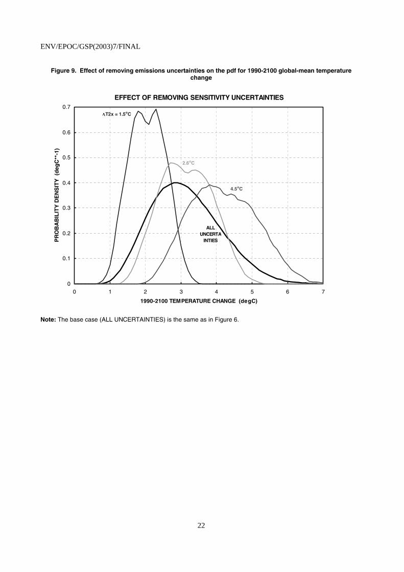
A similar situation arises in the case of climate sensitivity uncertainties. Figure 9 (see also Table 1) shows uncertainties in 1990-2100 global-mean warming for three different values of the climate sensitivity. For low and high sensitivities, the position of the pdf is changed radically from the general case, but the spread of the pdf remains large – due primarily to emissions uncertainties.


19

Figure 7. Effect of removing carbon-cycle model uncertainties on the pdf for 1990-2100 global-mean temperature change

EFFECT OF REMOVING CARBON CYCLE UNCERTAINTIES

0

0.05

0.1

0.15

0.2

0.25

0.3

0.35

0.4

0.45

0 1 2 3 4 5 6 7

1990-2100 TEMPERATURE CHANGE (degC)

PR

OB

AB

ILIT

Y D

EN

SIT

Y (

deg

C**

-1)

MEDIAN CO2 ONLY

ALL UNCERTAINTIES

Note: The base case (ALL UNCERTAINTIES) is the same as in Figure 6.


20

Table 1. Sources and magnitudes of uncertainties

EXPERIMENT

90% CONF. INT.

(degC)

RANGE (degC)

RANGE REL. TO ‘ALL’

UNCERTS’ ALL UNCERTS

1.683 – 4.874

3.191

1.000

MEDIAN Kz

1.686 – 4.855

3.169

0.993

MEDIAN AEROSOL

1.705 – 4.871

3.166

0.992

MEDIAN CO2

1.679 – 4.730

3.051

0.956

EMIS. = B1

1.187 – 2.971

1.783

0.559

EMIS. = A1B

1.821 – 4.081

2.260

0.708

EMIS. = A1FI

2.805 – 5.796

2.991

0.937

�T2x = 1.5oC

1.251 – 2.864

1.613

0.505

�T2x = 2.6oC

1.985 – 4.353

2.369

0.742

�T2x = 4.5oC

2.737 – 5.743

3.006

0.942

Notes: 90% confidence intervals and interval ranges for 1990-2100 global-mean temperature change for different uncertainty factor combinations. ALL UNCERTS gives the results when all uncertainties are accounted for, duplicating values given in Wigley and Raper (2001). MEDIAN Kz refers to vertical diffusivity in the model, and means that ocean mixing uncertainties are ignored. MEDIAN AEROSOL uses only the best estimates of 1990 aerosol forcing. MEDIAN CO2 uses only best-estimate carbon cycle model parameters (including those that quantify fertilization and climate feedbacks). The last six rows use single values for either the emissions scenario or the climate sensitivity.


21

Figure 8. Effect of removing emissions uncertainties on the pdf for 1990-2100 global-mean temperature change

EFFECT OF REMOVING EMISSIONS UNCERTAINTIES

0

0.1

0.2

0.3

0.4

0.5

0.6

0.7

0.8

0 1 2 3 4 5 6 7


PR

OB

AB

ILIT

Y D

EN

SIT

Y (

deg

C**

-1)

ALL UNCERTAINTIES

B1

A1B

A1FI



22

Figure 9. Effect of removing emissions uncertainties on the pdf for 1990-2100 global-mean temperature change

EFFECT OF REMOVING SENSITIVITY UNCERTAINTIES

0

0.1

0.2

0.3

0.4

0.5

0.6

0.7

0 1 2 3 4 5 6 7


PR

OB

AB

ILIT

Y D

EN

SIT

Y (

deg

C**

-1)

ALL UNCERTA

INTIES

�T2x = 1.5oC

2.6oC

4.5oC



23

6. SPATIAL PATTERNS OF CLIMATE CHANGE

Figures 6-9 show uncertainties in global-mean temperature projections for the no-climate-policy case. It should be noted that Figure 8 gives some important insights into the effects of policy. For example, one could suppose that the B1 scenario was achieved by implementing policies against the A1B scenario as a no-policy baseline. If this were so, then there would be clear benefits, since the median of the global-mean temperature pdf is shifted substantially towards lower warming. However, the spread of the pdf is reduced only minimally, a result that will apply to any policy case.

It is, of course, impossible to make a detailed assessment of the benefits, in terms of avoided impacts, of any mitigation policy using just global-mean temperature. The impacts of climate change occur at the local to regional level, and depend on many variables in addition to temperature. Because of this, and because of the uncertainties that surround projections of climate change at the regional level that will be described below, quantifying benefits is a daunting task. It is made even more difficult by the fact that most impacts models have large inherent uncertainties that compound uncertainties in their inputs.

The focus of this Section will be on uncertainties in the regional climate change signal that might arise from a mitigation policy. In reality, any such signal will be embedded in the noise of the climate system’s natural variability. For a given scenario, this adds another element of uncertainty. While natural variability is ignored here, it may be that it cannot be ignored in some impacts sectors. For example, in ecosystem impacts where changes in disturbance frequency can be of paramount importance, it may be essential to express these impacts in probabilistic terms generated by considering ensemble means spanning a range of (unpredictable!) future natural variability realizations. These variability issues make the problem of assessing uncertainties even more difficult. Indeed, even when restricting the discussion to a deterministic signal (i.e., ignoring the effects of internally-generated variability or noise), there has been little work of any value on quantifying uncertainties in regional climate.

So, how do we quantify these uncertainties in regional climate? One approach is to compare results from different models. To facilitate this, we employ the scaling method developed by the present author and first described in Santer et al. (1990). The fundamental assumption of this method is that future changes in climate may be decomposed into global-mean and spatial pattern components. Instead of considering the ‘raw’ patterns of climate change, therefore, we consider patterns of change per unit (1oC) of global-mean warming (which we refer to as ‘normalized’ patterns). This has many advantages, not least that it allows us to compare results from models that have very different climate sensitivities. Normalization essentially factors out the effects that are directly related to climate sensitivity differences. We can then consider the effects of sensitivity uncertainties separately at the global-mean level, as done in the preceding Sections, and concentrate on the underlying patterns of regional climate. By quantifying inter-model differences in the normalized patterns of change we obtain more fundamental insights into regional uncertainties.

Here, I use coupled atmosphere/ocean GCM results from the CMIP model-intercomparison project (Covey et al., 2002). The CMIP project has compiled data sets for unforced (‘control run’) experiments and for a standard forced (‘perturbation’) experiment for most of the world’s AOGCMs. (The perturbation experiment is one in which CO2 is increased at a compound rate of 1% per year corresponding closely to a linear increase in radiative forcing.)


24

In interpreting the CO2 increase results, it is important to define the signal correctly. A problem here is that, in terms of the spatial patterns of climate change, many AOGCMs show a significant ‘drift’. In other words, if the model is run in control mode (i.e., not subject to any external forcing), and even if the model’s global-mean temperature exhibits no long-term trend under such circumstances, the patterns of climate change may show substantial trends on the 100-year timescale. If this is the case, comparing future and initial climate states in a perturbation experiment (referred to as the Definition 1 method for defining the signal; Santer et al., 1994) will not give the true signal, but will give a mix of signal plus drift. To account for this, a standard procedure is to compare the perturbation experiment with a parallel control run (with both starting with the same initial conditions). If the drift is common to both, and there is strong evidence from tests with AOGCMs that it is, then subtracting the control run from the perturbation experiment will give a better estimate of the underlying signal. This is referred to as the Definition 2 method, and is the method employed here.

Normalized signals for annual-mean temperature and precipitation change, averaged over 17 AOGCMs, are shown in Figure 10. (Note that annual means are used here simply for illustrative purposes. Seasonal results would be of more direct relevance for impacts, but to span the seasons would have required four times as many maps. The information given here comes from the user-friendly software package ‘MAGICC/SCENGEN’, obtainable from the author, that allows the user to produce a wide range of similar results.)

Figure 10 shows a number of well-realized features: amplified warming in high northern latitudes; warming minima in the North Atlantic and around Antarctica associated with regions where deep water production occurs; increased precipitation over the tropical oceans and in high latitudes; and reduced precipitation in the subtropics (which are already dry) and around the Mediterranean. In most areas, the model-average changes in precipitation are quite small (less 3% change per degree C of global-mean warming), but this statistic hides large differences between the seasons and between models.

Uncertainties can be quantified by comparing these normalized signal patterns with the ‘noise’ of inter-model variability (i.e., by dividing the signal by the inter-model standard deviation on a grid point by grid point basis to form patterns of an inter-model signal-to-noise ratio (SNR)). These results are also shown in Figure 10 – also from MAGICC/SCENGEN. High SNR values frequently occur where the signal is large; although high SNR may also occur where the signal is small, but inter-model differences are even smaller. Low SNR generally means that model results differ widely.

In standard statistical terms, an SNR above 2 would indicate that the model-mean signal was statistically significant at the 5% level – i.e., that there was only one chance in 20 that the signal was zero (using a two-tail test). For temperature changes, SNR values exceed 2 for all regions except those around and downwind of the regions where deep water formation occurs. Low SNR values in these regions reflect smaller signals (see Figure 10) and larger differences between models. In contrast, for precipitation, SNR values are less than 2 for most of the globe. The exceptions are the high latitude regions where the signals are highest (Figure 10). Interestingly, there is some indication that the regions where we can have most confidence in the temperature change signals are also the regions where we have least confidence in precipitation signals. The temperature and precipitation SNR patterns are negatively correlated, but the pattern correlation is not high, about -0.4.

In practical terms, however, we might accept a much less stringent significance level. An SNR of +1 corresponds to the 16% significance level (one-tail test) and a probability of only one in six that the signal is zero or less. This would not be enough to satisfy normal statistical testing criteria, but, since there is still a high likelihood of a non-zero change, such SNR values may be of considerable ‘significance’ to the policy maker.


25

The phraseology used here suggests an alternative way of presenting SNR results. Instead of SNR values, if one assumes the distribution of models results to be Gaussian, then one can use the model mean and inter-model variability to calculate the probability of a change exceeding a specified threshold, such as the probability of a precipitation increase (where the threshold is zero) – see Santer et al. (1990). MAGICC/SCENGEN presents results in this way as well as through SNR values.

Would such a result (i.e., an SNR value around 1, or a probability of 84% that precipitation would increase) warrant action by a policy maker? Deciding on an SNR or probability threshold in the decision-making context depends on what is judged to be an acceptable risk. This in turn depends on the costs associated with two types of error relative to the benefits of action, responding to a supposed climate change signal when the true signal is zero, and failing to respond when there is a substantially non-zero true signal.


26

Figure 10. Model-average patterns of normalized annual-mean temperature change (i.e., changes per 1oC global-mean warming)

Notes: Averaged over 17 models from the CMIP data base for 1% compound CO2 increase perturbation experiments (Definition 2 changes) – top map, and corresponding inter-model signal-to-noise ratios (model-mean normalized change divided by inter-model standard deviation) – bottom map.


27

Figure 10 (continued)

Notes: Averaged over 17 models from the CMIP data base for 1% compound CO2 increase perturbation experiments (Definition 2 changes) – top map, and corresponding inter-model signal-to-noise ratios (model-mean normalized change divided by inter-model standard deviation) – bottom map.


28

7. TEMPERATURE PROJECTION UNDER CO2 STABILIZATION

In Section 2 I considered the SRES no-climate-policy emissions scenarios and showed, as policy examples, the WRE CO2 concentration stabilization profiles and the implied emissions requirements. Sections 3, 4 and 5 considered climate changes under the no-policy scenarios. Here I consider climate changes under the WRE policy scenarios. Although Article 2 of the UNFCCC has as its goal stabilization of all anthropogenic greenhouse gases, I will consider only the effects of CO2 stabilization here. Very little work has been done on the climate implications of multi-gas stabilization scenarios.

Non-CO2 gases cannot be ignored, however. To isolate the effects of CO2 stabilization I assume just a single scenario for non-CO2 gases, namely the P50 scenario used as a baseline for the updated WRE profiles. P50 emissions, however, are specified only to 2100, while the CO2 concentration profiles go to 2250 and beyond. In order to give climate projections to 2250, I therefore assume emissions of non-CO2 gases to remain constant at the 2100 level given in the P50 scenario. The radiative forcing from these gases therefore increases after 2100, albeit only slightly.

To further constrain the analysis I consider only a single set of climate model parameters, a climate sensitivity of 2.5oC and ‘best guess’ values for all other parameters (i.e., the values used in the IPCC TAR).

Figure 11 shows changes in global-mean temperature for the stabilization cases considered in Figure 3, together with the constant 2000-level fossil CO2 emissions case. There are a number of points to note. First, the greatest separation is between the 450ppm and 550ppm cases, while the least is between the 650ppm and750ppm cases. This results mainly from the logarithmic dependence of CO2 radiative forcing on concentration, which means that as the CO2 level increases, the forcing increment for a 100ppm concentration increment decreases. Second, although CO2 concentrations stabilize in all cases (as early as 2100 in the WRE450 case), warming continues beyond 2250. This is partly due to the influence of the non-CO2 gases, and partly because of the large thermal inertia of the climate system. Third, even though the emissions in the CO2 stabilization cases are much less than in the baseline P50 case (see Figure 4), the reduction in warming achieved through these emissions reductions is relatively small. For example, in 2100 the baseline emissions level is 17.57GtC/yr, while the WRE550 emissions level is approximately 60% less than this at 6.85GtC/yr. The corresponding 1990-2100 warmings are 2.81oC for the baseline and 2.22oC for WRE550 (only 20% less). This again is a consequence of the thermal inertia of the climate system.

Finally, by 2250 warming under the overshoot 550ppm concentration pathway has returned almost to the standard 550ppm case. Overshoot allows emissions to rise 14% above the no-overshoot case, while the maximum increase in global-mean temperature change relative to 1990 is somewhat less, around 10%. It is likely that the overshoot case would lead to reduced mitigation costs, while the attendant increased warming would certainly lead to a reduction in the benefits of averted climate change. This raises the question of whether the reduced mitigation costs are enough to offset the reduction in climate-change benefits. While answering this question is beyond the scope of the present work, it is clear that overshoot CO2 stabilization pathways warrant further investigation.


29

Figure 11. Global-mean temperature projections for the CO2 concentration pathways shown in Figure 3

TEMPERATURE CHANGES FOR STABILIZATION PATHWAYS

0

0.5

1

1.5

2

2.5

3

3.5

4

1990 2010 2030 2050 2070 2090 2110 2130 2150 2170 2190 2210 2230 2250YEAR

GL

OB

AL

-ME

AN

TE

MP

ER

AT

UR

E C

HA

NG

E (

deg

C)

WRE450

WRE550

WRE650

WRE750

P50 BASELINE

CONST EFOSS .

OVERSHOOT

�T2x = 2.5 degC

Notes: Results are for a climate sensitivity of 2.5oC and IPCC TAR central estimates of all other model parameters. Non-CO2 emissions are assumed to follow the P50 scenario to 2100 and remain constant thereafter. Black diamonds show the dates at which CO2 concentrations stabilize.


30

8. CONCLUSIONS

This paper considers future changes in climate and the uncertainties in these changes at the global-mean and spatial pattern levels for both no-climate-policy and policy cases. Where possible, a probabilistic approach is used.

Emissions projections, as the primary drivers of anthropogenic climate change, are considered first, for both the no-policy case (characterized by the SRES scenarios) and the policy case (following the WRE CO2 stabilization profiles). The most important feature of the WRE profiles is that, for stabilization targets above about 450ppm, they do not require immediate reductions in emissions below the baseline no-policy case. Eventually, emissions must drop below present levels, but, depending on the chosen stabilization target, they may remain above present levels for decades to more than a century. The possibility of following an overshoot pathway to stabilization (where the peak concentration exceeds the eventual stabilization target) is introduced.

Probabilistic projections for global-mean temperature under the no-policy assumption produced by Wigley and Raper (2001) are broken down by uncertainty factor in order to quantify the relative importance of different sources of uncertainty (ocean mixing, aerosol forcing, the carbon cycle, emissions, and the climate sensitivity). A new method is employed to do this: removal of individual sources of uncertainty and comparison of the resulting pdf with that based on the full uncertainty assessment. Small changes in the pdf imply that uncertainties in the factor removed are relatively unimportant. For temperature changes over 1990-2100, emissions and climate sensitivity uncertainties are shown to be by far the most important. Removing either emissions or sensitivity uncertainties, however, has only a small effect on the spread of the global-mean temperature pdf – in other words, the effect of emissions or sensitivity uncertainties alone is similar to their combined effect.

Uncertainties in the regional patterns of climate change are examined using normalized patterns of change (i.e., patterns of change per 1oC global-mean warming). This method, proposed many years ago but rarely used, allows us to separate the effects of climate sensitivity uncertainties from those inherent in the patterns of change. Pattern uncertainties are based on the differences between 17 AOGCMs in the CMIP data base, and quantified using a signal-to-noise ratio (model-mean signal divided by inter-model standard deviation). Temperature uncertainties are shown to be greatest at high latitudes and least in low latitudes, while precipitation shows the opposite pattern.

For mitigation policies, Article 2 of the UNFCCC implies that both mitigation costs and the benefits of averted climate change should be considered. On the cost side, for CO2, it is sufficient to consider only changes at the global-mean level. For benefits, regional climate change information is needed. This almost certainly makes the assessment of benefits more difficult than the assessment of costs.


31

9. REFERENCES

Andronova, N.G. and Schlesinger, M.E., 2001: Objective estimation of the probability density function for climate sensitivity. Journal of Geophysical Research 106, 22605-22611.

Covey, C., Achuta Rao, K.M., Cubasch, U., Jones, P.D., Lambert, S.J., Mann, M.E., Phillips, T.J. and Taylor, K.E., 2003: An overview of results from the Coupled Model Intercomparison Project (CMIP), Global and Planetary Change (in press).

Cubasch, U., and Meehl, G.A., 2001: Projections for future climate change. Climate Change 2001: The Scientific Basis, (eds. J. T. Houghton, et al.), Cambridge University Press, Cambridge, U.K., 525–582.

Grübler, A., 1998: A review of global and regional sulphur emission scenarios. Mitigation and Adaptation Strategies for Global Change 3, 383-418.

Harvey, L.D.D., Gregory, J., Hoffert, M., Jain, A., Lal, M., Leemans, R., Raper, S.B.C., Wigley, T.M.L. and de Wolde, J., 1997: An introduction to simple climate models used in the IPCC Second Assessment Report: IPCC Technical Paper 2 (eds. J.T. Houghton, L.G. Meira Filho, D.J. Griggs and M. Noguer), Intergovernmental Panel on Climate Change, Geneva, Switzerland, 50 pp.

Hoffert, M.I., Caldeira, K., Jain, A.K., Haites, E.F., Harvey, L.D.D., Potter, S.D., Schlesinger, M.E., Schneider, S.H., Watts, R.G., Wigley, T.M.L. and Wuebbles, D.J., 1998: Energy implications of CO2 stabilization. Nature 395, 881–884.

Hoffert, M.L., Caldiera, K., Benford, G., Criswell, D.R., Green, C., Herzog, H., Jain, A.K., Kheshgi, H.S., Lackner, K.S., Lewis, J.S., Lightfoot, H.D., Mannheimer, W., Mankins, J.C., Mauel, M.E., Perkins, L.J., Schlesinger, M.E., Volk, T. and Wigley, T.M.L., 2002: Advanced technology paths to global climate stability: Energy for a greenhouse planet. Science 298, 981-987.

Houghton, J.T., et al., Eds, 2001: Climate Change 2001: The Scientific Basis. Cambridge University Press, xxx pp.

Manne, A.S. and Richels, R.G., 2001: An alternative approach to establishing trade-offs among greenhouse gases. Nature 410, 675-677.

��(Special Report on Emissions Scenarios. Cambridge University Press, 570 pp.

Raper, S.C.B., Wigley, T.M.L. and Warrick, R.A., 1996: Global sea level rise: past and future. (In) Sea-Level Rise and Coastal Subsidence: Causes, Consequences and Strategies (eds. J. Milliman and B.U. Haq), Kluwer Academic Publishers, Dordrecht, The Netherlands, 11–45.

Santer, B.D., Wigley, T.M.L., Schlesinger, M.E. and Mitchell, J.F.B., 1990: Developing Climate Scenarios from Equilibrium GCM Results. Max-Planck-Institut für Meteorologie Report No. 47, Hamburg, Germany, 29 pp.

Santer, B.D., Brueggemann, W., Cubasch, U., Hasselmann, K., Hoeck, H., Maier-Reimer, E. and Mikolajewicz, U., 1994: Signal-to-noise analysis of time-dependent greenhouse warming experiments. Climate Dynamics 9, 267-285.


32

Schneider, S.H., 2001: What is dangerous climatic change? Nature 411, 17-19.

Schneider, S.H., 2003: Abrupt non-linear climate change, irreversibility and surprise (this volume).

Smith, J.B. and Hitz, S., 2003: Background paper: Estimating global impacts from climate change (this volume).

Smith, J.B., Schellnhuber, H.-J. and Mirza, M.M.Q., 2001a: Vulnerability to climate change and reasons for concern: A synthesis. (In) Climate Change 2001: Impacts, Adaptation, and Vulnerability, Contribution of Working Group II to the Third Assessment Report of the Intergovernmental Panel on Climate Change (eds. J. McCarthy, O. Canziana, D. Dokken and K. White), Cambridge University Press, Cambridge, U.K., 913–967.

Smith, S.J., Pitcher, H. and Wigley, T.M.L., 2001b: Global and regional anthropogenic sulphur dioxide emissions. Global and Planetary Change 29, 99-119.

Wigley, T.M.L., 1993: Balancing the carbon budget. Implications for projections of future carbon dioxide concentration changes. Tellus 45B, 409–425.

Wigley, T.M.L., 2002: Stabilization of CO2 and other greenhouse gas concentrations. Climatic Change (accepted for publication).

Wigley, T.M.L. and Raper, S.C.B., 1992: Implications for climate and sea level of revised IPCC emissions scenarios. Nature 357, 293–300.

Wigley, T.M.L. and Raper, S.C.B., 2001: Interpretation of high projections for global-mean warming. Science 293, 451-454.

Wigley, T.M.L., Richels, R. and Edmonds, J.A., 1996: Economic and environmental choices in the stabilization of atmospheric CO2 concentrations. Nature 379, 240–243.

Wigley, T.M.L., Smith, S.J. and Prather, M.J., 2002: Radiative forcing due to reactive gas emissions. Journal of Climate 15, 2690-2696.

Documents

Modelling climate change under no-policy and policy emissions pathways