364

1. Introduction

The importance of geomorphological processes and their impact on the archaeological record has been recognised for a long time (e.g. Butzer 1982). This has divided into two different, although related, areas of interest. Firstly the physical record itself, how areas of erosion, the movement of material and its subsequent deposition, can denude and cover archaeological remains (Waters and Kuehn 1996). The second area of interest is linked to past land use practices, considering what activities in the past may have caused erosion and colluviation, with much of the early work concentrating on the Chalk downlands of central southern England (Bell 1983). Such geomorphological activities are often recognised and discussed within the context of surface survey and the possible impact on surface and sub­surface archaeology (Bispham et al 2008).

There have been a series of computer­based attempts to model and visualise the geomorphological processes of colluviation and alluviation and their effects on archaeological distributions. For example, Miller’s (1996) pilot study of urban deposit modelling in York which used data from over 2,000 interventions to produce a visualisation of the Roman land surface. Burton and Shell (2000), working in the Fen edges of eastern England used over 1,100 boreholes with depths of alluvium, peat, sands and gravels to model

a series of relic landscapes. Of particular interest here is attempting to understand the movement of materials through the use of flow models, an early example of which is Wainwright and Thornes (1991) who developed a sediment transport model to look mainly at the movement of artefacts but also of sediments.

One of the most detailed discussions of erosional modelling within an archaeological context is Verhagen (1996) who details different sorts of models, including: qualitative and quantitative models which apply a formula; lumped and distributed models which have a spatial component; and static and dynamic models which have a temporal component through change, feedback loops, or time series mechanisms. The aim was to develop the first quantitative, distributed dynamic model for estimating upslope contributing areas and taking into account that water flow converges in channels. This work is relevant here because it emphasises the importance of DEM resolution and quality, and the problem of interpolation artefacts stopping ‘flow’. Also of interest is the emphasis on the importance of small­scale ‘local’ effects and the problems of generalised large-scale modelling.

The work described here is carried out within the AHRC funded project at the Universities of Bristol and Oxford under the auspices of the South Cadbury Environs Project. South Cadbury is a 7

Modelling Colluviation: Land Use and Landscape Change in the South Cadbury Environs

Gary lock1 – John pouNcett2

1,2 Institute of Archaeology, University of Oxford1gary.lock@arch.ox.ac.uk

2johnpouncett@ase-limited.co.uk

AbstractAn extensive programme of test-pitting has been carried out in the immediate vicinity of the Iron Age hillfort at South

Cadbury, Somerset, UK under the auspices of the South Cadbury Environs Project. The deposits of colluvium (hillwash)

and erosion surfaces recorded during the course of this test­pitting represent an ideal dataset with which to develop and

test a model for colluviation. Algorithms developed for the purposes of morphometric surface characterisation are used

to develop a model which seeks to both identify the areas which contribute to the accumulation of colluvium in individual

phases of activity, and manipulate the digital elevation model to reflect the cumulative impact of erosion and deposition in

successive phases of activity. The results are compared with test-pit data and help in understanding the development of the

landscape.

Keywordscolluviation, modelling, South Cadbury Environs Project

Proceedings of the 36th CAA Conference, Budapest, 2–6 April 2008

365

Modelling Colluviation: Land Use and Landscape Change in the South Cadbury Environs

hectare multi-vallate hillfort in Somerset, England, perhaps best known for its possible connections with King Arthur (Alcock 1995). Excavations undertaken at the site between 1966 and 1970 – both through the ramparts and within the interior of the hillfort – revealed a complex sequence of activity from the Later Bronze Age until the 5th and 6th centuries AD. Recent analysis has identified three main phases of activity: Early Cadbury (1,000 BC to 300 BC) – the first ramparts; Middle Cadbury (300 BC to AD 40/50) – the main occupation of the hillfort; and Late Cadbury (AD 40/50 to AD 400) – possible (re)use as Roman barracks (Barrett et al. 2000). The South Cadbury Environs Project aims to place the hillfort within a broader landscape context, particularly the development and evolution of the cultural landscape. This has involved two innovative GIS-

based approaches, the first using Network Analysis to date a complex of features identified through large-scale geophysics (Lock and Pouncett in press), and the current work realising that colluviation has had an important impact on understanding the cultural development of this landscape and on our ability to identify and interpret past activity.

2. Test-pitting data

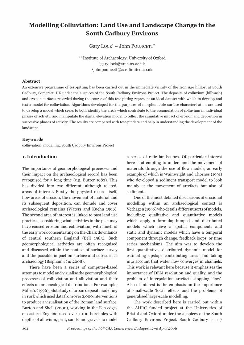
The study area is defined by a bounding rectangle 8km by 8km centred on South Cadbury hillfort (Fig. 1). Six localities within this study area (Localities 1, 1a, 2, 3, 4 and 5) have been intensively sampled (Tabor 2002, 13) and over 300 test-pits excavated, 170 containing colluvial deposits. The test-pits can be divided into two groups:

Fig. 1. Location map showing the study area for the South Cadbury Environs Project.

366

Gary lock – John pouncett

1. 1m by 1m test-pits excavated on a 100m grid to assess the variation of artefact densities and build a geomorphological map to aid the interpretation of the geophysical survey;

2. Targeted test-pits, at least 1m by 1m, excavated specifically to assess geophysical anomalies and obtain dating evidence.

The nature of the sampling strategy is such that the test­pits which contained colluvial deposits are clustered in the six localities rather than dispersed evenly across the study area. Any model based on the distribution of these colluvial deposits will be most accurate in the areas with the highest incidence of test-pits. The validity of the model developed here will consequently be assessed using data from three of the localities (Localities 2, 3 and 5).

Up to seven deposits of colluvium, with a maximum cumulative depth of 1.68m, were identified at each test­pit location, each assumed to correspond to a discrete episode of colluviation. Dates were assigned to individual episodes on the basis of artefact associations. A simplified version of the chronology established for the South Cadbury Environs Project (Leach and Tabor 1997, 8) was used to differentiate between six principal colluvial phases: Post Glacial, Early Prehistoric, Late Prehistoric, Romano-British, Mediaeval and Modern. Over half of the colluvial deposits which could be dated independently were associated with modern colluviation. Where more than one episode could be assigned to a single phase, the depths of colluvial deposits were aggregated.

By extracting the co­ordinates of the centroids of each of the test­pits it is possible to construct a point­provenance plot showing both the presence/absence of colluvial deposits and the cumulative depth of colluvium at each location. Morphometric surface characterisation can be used to identify the key topographic zones within which colluviation took place. Surface parameters can subsequently be used to weight these zones on the basis of their probable susceptibility to colluviation producing ‘colluvial zones’ which can be used to generate a continuous surface representing variability in the depth of colluvium.

3. Morphometric classification

Modelling of geomorphological processes is predominately raster­based and is heavily reliant upon the analysis and manipulation of digital

elevation models (DEMs). The model developed here is based on the Land-Form PROFILE DTMTM with a 10m resolution. A DEM model is a continuous surface representing variation in elevation relative to an absolute datum. The identification of topographic features is not possible on the basis of the absolute elevations of individual cells and is instead reliant upon the comparison of the elevation of a cell relative to the elevations of other cells in the DEM (Wood 1996).

Algorithms developed for this purpose are locally adaptive and typically employ a neighbourhood or ‘n x n’ window to compare the elevations of neighbouring cells. In the case of a ‘3 x 3’ window, the elevation of the cell at the centre of the window would be compared to the elevations of the eight adjacent cells. ‘n x n’ windows are routinely employed in the calculation of slope and aspect (Conolly and Lake 2006, 187-188). They can also be used for the purposes of identifying topographic features. Each cell within a DEM can be reclassified as one of six morphometric feature types (Wood 1996):

1. Pits – the cell at the centre of the window is lower than all of the adjacent cells;

2. Channels – the cells along the centreline of the window are lower than the cells either side of the centreline;

3. Passes – a channel where the cell at the centre of the window is higher than the other cells along the centreline;

4. Ridges – the cells along the centreline of the window are higher than the cells either side of the centreline;

5. Peaks – the cell at the centre of the window is higher than all of the adjacent cells;

6. Planes – the cells within the window form a horizontal or sloping planar surface.

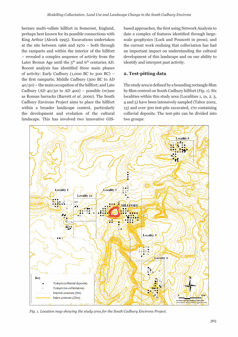
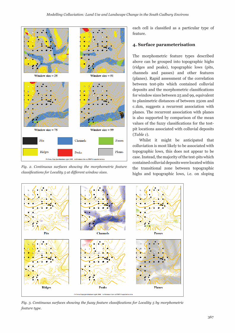
The classification of individual cells is scale dependent and will vary with window size (Fig. 2). Smaller window sizes respect local topographic features, while larger window sizes reflect the overall morphology of a DEM. Multiscalar approaches based on fuzzy features classes have been developed to address this issue (Fisher et al. 2004, 109–110). Morphometric classifications are generated using Landserf 2.3 (Wood 2007), for all window sizes within a specified range, and combined to create fuzzy classifications for each feature type (Fig. 3). The reclassified datasets contain numeric values between 0 and 1, which provide a measure of confidence that

367

Modelling Colluviation: Land Use and Landscape Change in the South Cadbury Environs

each cell is classified as a particular type of feature.

4. Surface parameterisation

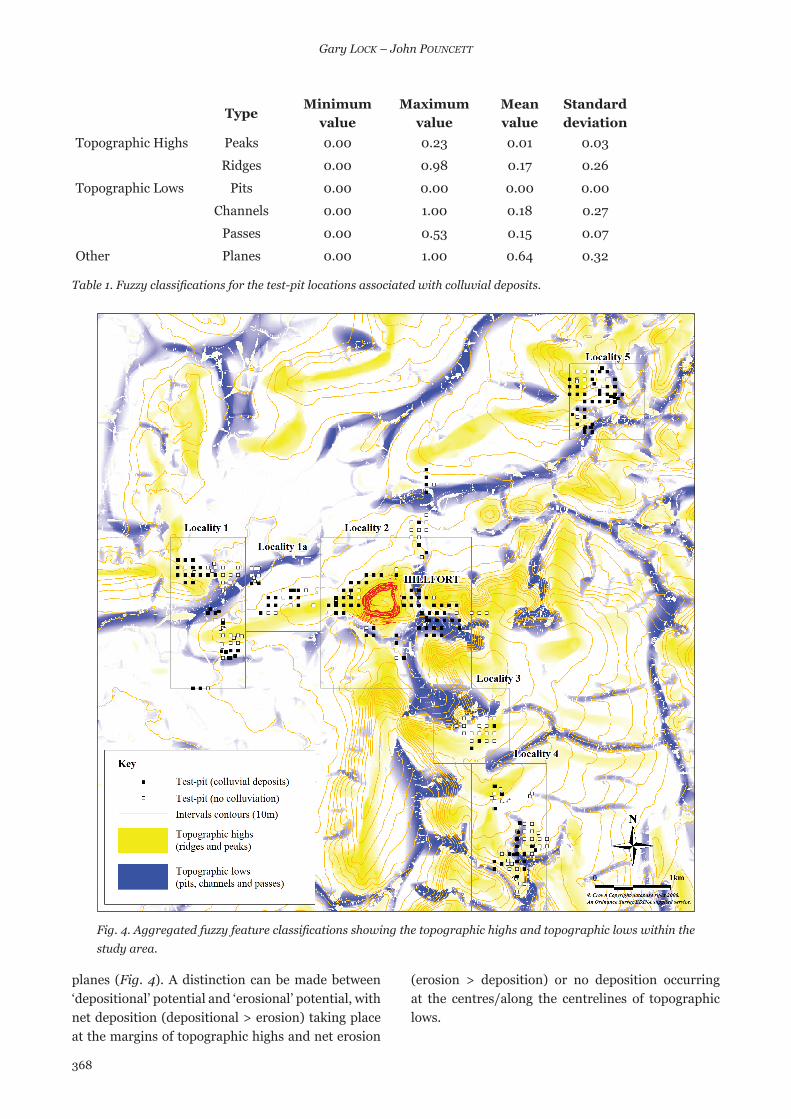
The morphometric feature types described above can be grouped into topographic highs (ridges and peaks), topographic lows (pits, channels and passes) and other features (planes). Rapid assessment of the correlation between test­pits which contained colluvial deposits and the morphometric classifications for window sizes between 25 and 99, equivalent to planimetric distances of between 250m and c.1km, suggests a recurrent association with planes. The recurrent association with planes is also supported by comparison of the mean values of the fuzzy classifications for the test-pit locations associated with colluvial deposits (Table 1).

Whilst it might be anticipated that colluviation is most likely to be associated with topographic lows, this does not appear to be case. Instead, the majority of the test-pits which contained colluvial deposits were located within the transitional zone between topographic highs and topographic lows, i.e. on sloping

Fig. 2. Continuous surfaces showing the morphometric feature classifications for Locality 5 at different window sizes.

Fig. 3. Continuous surfaces showing the fuzzy feature classifications for Locality 5 by morphometric feature type.

368

Gary lock – John pouncett

planes (Fig. 4). A distinction can be made between ‘depositional’ potential and ‘erosional’ potential, with net deposition (depositional > erosion) taking place at the margins of topographic highs and net erosion

(erosion > deposition) or no deposition occurring at the centres/along the centrelines of topographic lows.

TypeMinimum

valueMaximum

valueMeanvalue

Standard deviation

Topographic Highs Peaks 0.00 0.23 0.01 0.03

Ridges 0.00 0.98 0.17 0.26

Topographic Lows Pits 0.00 0.00 0.00 0.00

Channels 0.00 1.00 0.18 0.27

Passes 0.00 0.53 0.15 0.07

Other Planes 0.00 1.00 0.64 0.32

Table 1. Fuzzy classifications for the test-pit locations associated with colluvial deposits.

Fig. 4. Aggregated fuzzy feature classifications showing the topographic highs and topographic lows within the study area.

369

Modelling Colluviation: Land Use and Landscape Change in the South Cadbury Environs

Having identified the topographic zones within which colluviation is taking place, it is necessary to both isolate sloping planes and weight the points on those planes where the ‘depositional’ potential is greatest. A topographic surface can be described using a series of terrain parameters (Evans 1972), including elevation, slope and curvature. Slope and curvature are 1st and 2nd order differentials of elevation respectively. Both parameters were calculated in Landserf 2.3, using a window size of 25 in order to eliminate interpolation artefacts identified in the DEM and minimise the impact of localised topographic features.

‘Erosional’ potential is proportionate to slope, with erosion more likely to occur on steep slopes. Conversely, ‘depositional’ potential is inversely

proportionate to slope, with deposition more likely to occur on shallow slopes. Although a slope with a particular inclination may correspond to either a topographic high or a topographic low, the ‘erosional’ or ‘depositional’ potential will not be the same in both instances. In the case of a sloping plane, ‘erosional’ potential and ‘depositional’ potential are likely to be greatest at the top of the slope and the base of the slope respectively.

The upper reaches and lower reaches of a slope can be defined in relation to the contiguous topographic highs and topographic lows, and can be characterised respectively by positive curvature (convex slopes) and negative curvature (concave slopes). There is no standard definition of curvature (Woods 1996). The definition used here (longitudinal

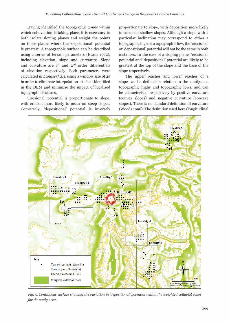
Fig. 5. Continuous surface showing the variation in ‘depositional’ potential within the weighted colluvial zones for the study area.

370

Gary lock – John pouncett

curvature) maximises the effect of gravity and, as such, is considered to be appropriate for the purposes of modelling colluviation.

5. Modelling colluviation

Colluviation is most likely to occur on moderate slopes and the cumulative depth of colluvial deposits is likely be greater on concave slopes than on convex slopes. Little or no deposition is likely to take place on shallow slopes on hill tops or in valley bottoms, or on steep slopes close to a ‘tip point’ ­ any point on a sloping plane where the ‘erosional’ potential is equal to the ‘depositional’ potential, usually the steepest section of the midslope. Either side of ‘tip points’, ‘depositional’ potential will decrease towards the apex of the convex slope and increase towards the apex of a concave slope.

Raster algebra was used to combine the fuzzy feature classifications and surface parameters in order to develop a model for colluviation based on weighted surfaces. Three raster datasets were initially derived from the DEM, representing ‘planarity’, slope and longitudinal curvature. The datasets for slope and longitudinal curvature were subsequently reclassified to create separate raster datasets for concave slopes (longitudinal curvature < 0.00) and convex slopes

(longitudinal curvature > 0.00). In both instances, the slope data was clipped to the range of values for test­pit locations associated with colluvial deposits (slope > 0.43º and slope < 12.88º).

The reclassified datasets for concave slopes and convex slopes were standardised with cell values, between 0 and 1, centred on the mean. A linear relationship between ‘depositional’ potential and slope was assumed for the purposes of developing and testing the model presented here. Linear and inverse linear functions were applied to mimic the increase and decrease in ‘depositional’ potential either side of the apex of convex and concave slopes. Arbitrary weights were then applied to the transformed values to reflect the probability that colluviation is more likely to take place on concave slopes (weight = 10) than on convex slopes (weight = 1).

A continuous surface showing weighted colluvial zones for the study area (Fig. 5) was produced by multiplying the cell values of the fuzzy feature classification for planes by the values of the cells for aggregated concave and convex slopes. Individual continuous surfaces were then interpolated using the aggregated depth of colluvial deposits for each phase of colluviation. Test-pit locations with no evidence of colluviation (depth = 0) were included in the point data used to interpolate the continuous surfaces.

Finally, the interpolated values were multiplied by the cell values for the weighted colluvial zones to create a continuous surface showing variation in the depth of colluvium.

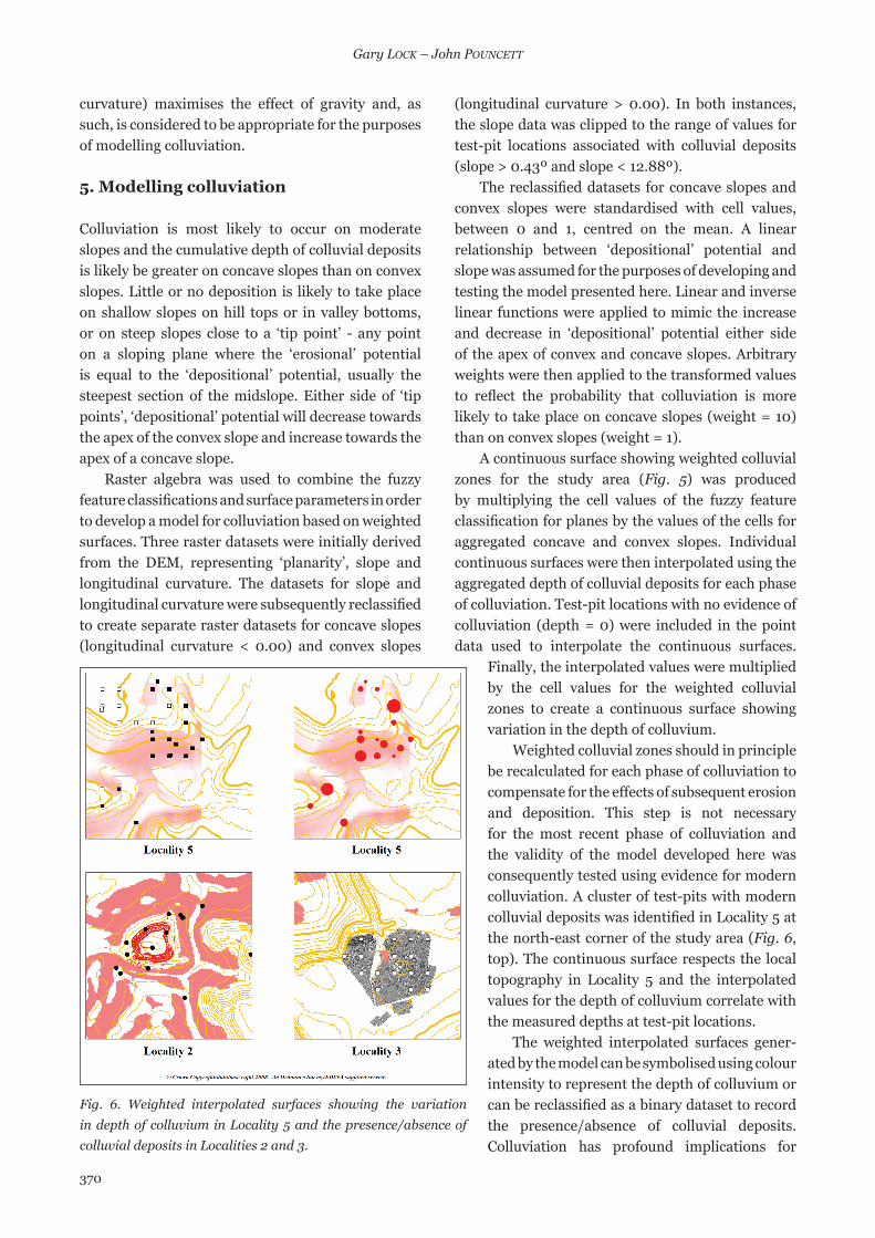
Weighted colluvial zones should in principle be recalculated for each phase of colluviation to compensate for the effects of subsequent erosion and deposition. This step is not necessary for the most recent phase of colluviation and the validity of the model developed here was consequently tested using evidence for modern colluviation. A cluster of test-pits with modern colluvial deposits was identified in Locality 5 at the north­east corner of the study area (Fig. 6, top). The continuous surface respects the local topography in Locality 5 and the interpolated values for the depth of colluvium correlate with the measured depths at test-pit locations.

The weighted interpolated surfaces gener­ated by the model can be symbolised using colour intensity to represent the depth of colluvium or can be reclassified as a binary dataset to record the presence/absence of colluvial deposits. Colluviation has profound implications for

Fig. 6. Weighted interpolated surfaces showing the variation in depth of colluvium in Locality 5 and the presence/absence of colluvial deposits in Localities 2 and 3.

371

Modelling Colluviation: Land Use and Landscape Change in the South Cadbury Environs

archaeological visibility. The reclassified data shows little or no correlation between deposits of colluvium and the distribution of known archaeological sites close to the Iron Age hillfort in Locality 2 (Fig. 6, bottom left) or the area where archaeological features and deposits have been identified through geophysical survey at Sigwells in Locality 3 (Fig. 6, bottom right).

6. Conclusion

This work has demonstrated the potential for modelling archaeological visibility and landscape change through the differentiation of the topographic zones within which colluviation occurred between successive phases of activity and possible correlation with wider evidence for landscape use. The proposed methodology of morphometric classification and surface parameterisation makes no assumptions about topographic zones within which colluviation occurred and the test pitting data provides independent validation for the modelling of colluvial deposits. Further work will include flow models and hydrological analysis (Conolly and Lake 2006, 256–260), modifying the DEM using cut and fill methods to mitigate against the impact of each phase of colluviation, interpolating a surface for the cumulative depth of all colluvial deposits and the identification of active/inactive colluvial zones for individual phases of colluviation.

References

Alcock, Leslie (1995). Cadbury Castle, Somerset: the early mediaeval archaeology. Cardiff: University of Wales Press.

Barrett, John, Freeman, Philip and Woodward Ann (1995). Cadbury Castle, Somerset: the later prehistoric and early historic archaeology. London: English Heritage.

Bell, Martin (1983). Valley sediments as evidence of prehistoric land-use on the South Downs. Proceedings of the Prehistoric Society 49, 119–150.

Bispham, Edward, Swift, Keith and Wolff, Tico (2008). ‘What lies beneath’: ploughsoil assemblages, the dynamics of taphonomy and the interpretation of field walking data. In: Lock, Gary and Faustoferri, Amalia (eds.) Archaeology and landscape in central Italy. Papers in memory of John. A. Lloyd. (Oxford

University School of Archaeology Monograph 69). Oxford: Oxford University School of Archaeology, 53–76.

Burton, Nick and Shell, Colin (2000). GIS and visualising the palaeoenvironment. In: Lockyear, Kris, Sly, Timothy and Mihăilescu-Bîrliba, Virgil (eds.) CAA96 Computer Applications and Quantitative Methods in Archaeology. (BAR International Series 845). Oxford: British Archaeological Reports, 81–90.

Butzer, Karl (1982). Archaeology as human ecology. New York: Cambridge University Press.

Conolly, James and Lake, Mark (2006). Geo-graphical Information Systems in Archaeology. Cambridge: Cambridge University Press.

Evans, Ian (1972). General geomorphometry, derivatives of altitude, and descriptive statistics. In: Chorley, Richard (ed.) Spatial Analysis in Geomorphology. London: Methuen, 17–90.

Fisher, Peter, Wood, Jo and Cheng, Tao (2004). Where is Helvellyn? Fuzziness of multiscale landscape morphometry. Transactions of the Institute of British Geographers 29(1), 106–128.

Leach, Peter and Tabor, Richard (1997). The South Cadbury Environs Project. Proceedings of the Somerset Archaeological and Natural History Society 139, 47–57.

Lock, Gary and Pouncett, John (in press). Closest facility analysis: integration of geophysical and test-pitting data from the South Cadbury Environs Project. In: Herzog, Irmela, Lambers, Karsten and Posluschny, Axel (eds.) Layers of perception: advanced technological means to illuminate our past CAA2007. Berlin: Deutsche Archäologische Institut.

Miller, Paul (1996). Digging deep: GIS in the city. In: Kamermans, Hans and Fennema, Kelly (eds.) Interfacing the Past. Computer Applications and Quantitative Methods in Archaeology CAA95. (Analecta Praehistorica Leidensia 28). Leiden: University of Leiden, 369–378.

Tabor, Richard (ed.) (2002). South Cadbury Environs Project: interim fieldwork report, 1998–2001. Bristol: University of Bristol, Centre for the Historic Environment.

Verhagen, Philip (1996). The use of GIS as a tool for modelling ecological change and human occupation in the Middle Aguas valley (S.E. Spain). In: Kamermans, Hans and Fennema, Kelly (eds.) Interfacing the Past. Computer Applications and Quantitative Methods in

372

Gary lock – John pouncett

Archaeology CAA95. (Analecta Praehistorica Leidensia 28). Leiden: University of Leiden, 317–324.

Wainwright, John and Thornes, John (1991). Computer and hardware modelling of archaeological sediment transport on hillslopes. In: Lockyear, Kris and Rahtz, Sebastian (eds.) Computer Applications and Quantitative Methods in Archaeology 1990. (BAR International Series 565). Oxford: British Archaeological Reports, 183–194.

Waters, Michael and Kuehn, David (1996). The geoarchaeology of place: the effect of geological processes on the preservation and interpretation of the archaeological record. American Antiquity 61(3), 483–497.

Wood, Jo (1996). Scale-based characterisation of digital elevation models. In: Parker, David (ed.) Innovations in GIS 3. London: Taylor & Francis, 163–75.

Wood, Jo (2007). Landserf: visualisation and analysis of terrain models. (http://www.soi.city.ac.uk/~jwo/landserf/ landserf230/index.html). Accessed 27th May 2008.