Modelling cyclone hazard in Bangladesh - ITC · Modelling cyclone hazard in Bangladesh 30 ILWIS Applications Guide 3.1 Introduction Despite the fact that the Bangladesh Government

ILWIS Applications Guide 29

CHAPTER 3

Modelling cyclone hazard inBangladesh

By:M.C.J. Damen and C.J. van WestenDepartment of Earth Resources Surveys,International Institute for Aerospace Survey and Earth Sciences (ITC),P.O. Box 6, 7500 AA Enschede, The Netherlands.Tel: +31 53 4874283, Fax: +31 53 4874336, e-mail: [email protected]: +31 53 4874263, Fax: +31 53 4874336, e-mail: [email protected]

Summary

This exercise deals with the use of GIS for cyclone hazard zonation, in a study areaSouth of Chittagong, Bangladesh, using data of the April 1991 cyclone. Theexercise will produce several maps of the expected number of casualties per villageand population category caused by cyclone flood events with return periods of 5, 10,20 and 50 years. Prior to this, maps have to be made of the flood depth per returnperiod, the population density and the vulnerability of the population to flooding.For the calculation of the flood depths, use will be made of a digital terrain modeland a linear flood-decay model.

Getting started

The data for this case study are stored on the ILWIS 2.1 CD-ROM in the directoryd:\appguide\chap03. If you have already installed the data on your hard-disk, youshould start up ILWIS and change to the subdirectory where the data files for thischapter are stored, c:\ilwis21\data\appguide\chap03. If you did not install thedata for this case study yet, please run the ILWIS installation program (see ILWISInstallation Guide).

F • Double-click the ILWIS program icon in the ILWIS program group.

• Change the working drive and the working directory until you are inthe directory c:\ilwis21\data\appguide\chap03.

Modelling cyclone hazard in Bangladesh

30 ILWIS Applications Guide

3.1 IntroductionDespite the fact that the Bangladesh Government issued warnings of the impendingflooding, for the April 1991 cyclone, through its Cyclone Preparedness Program,and about 3 million people could have been moved to safety, many inhabitantsremained behind to protect their property. During this disaster an estimated138.000 people were killed and large numbers of houses, agricultural lands andinfra-structural works were destroyed. Hundreds of schools were damaged andseven to eight thousand vessels were lost. Almost every bridge and culvert in thearea was damaged and roads were washed out.

Within two days government air drops of food and medicine started, but they werehampered by continuing bad weather associated with the storm. Nearly two weekshad passed before massive international aid could react to the disaster and it wasmany months before the area returned to normal.

The Banskhali study area is situated in the East of Bangladesh, South of the city ofChittagong. Area maps and attribute tables of the geomorphology, villagepopulation, the Union-districts, roads, embankments, cyclone shelters, and theelevation of the terrain with cm accuracy are provided. Also available are a LandsatThematic Mapper and SPOT panchromatic image. For a general introduction youcan make use of a geomorphologic overview map of the whole coastal zone ofBangladesh as well as ten ground photographs of the Banskhali area.

Some GIS files are derived from:

− Sirajur Rahman Khan (1995) - “Geomorphic Characterization of cyclonehazards along the coast of Bangladesh”, ITC-MSc study.

Other important information on the area has been taken from:

− “GIS technology for disaster management”, prepared by the Irrigation supportproject for Asia and the Near East (ISPAN), as contribution to the BangladeshFlood Action Plan (FAP19); and

− Stephen T. Ray (1994) - “An assessment of the potential of applying GIS totwo aspects of disaster management: Storm surge modeling and Cycloneshelter analysis”. MSc thesis of the University of Nottingham, UK

Additional background information on the cyclones is given in the Appendix. Thisappendix is available in Word format in the same directory as the data files. It isrecommended to read the text in the Appendix first before starting the exercise.

Structure of the exercises

− In sections 3.2 and 3.3 all the files necessary for the exercise are given.

− Information is given on the display of the different data layers, such assegment, vector, point and raster maps, attribute tables, etc.

− In section 3.4 the analysis of historical cyclone events will be explained byusing graphs of surge height, wind speed, number of casualties, etc. It is alsorecommended to read the Appendix (Wordfile appendix.doc).



− In section 3.5 cyclone surge hazard maps will be made for different returnperiods of the cyclone events. Use is made of a linear decay model of the flooddepth. Repeated calculation can be done with an ILWIS Script.

− Section 3.6 explains the vulnerability and risk analysis. First the vulnerabilitiesof the total population to certain flood depths are estimated using data of the1991 cyclone event. The number of potential casualties per village for surgeflooding with a certain return period will also be calculated. Finally the surgeflood risk will be determined for each village and population category, basedon the formula:

Risk=(Probability of occurrence)*(Vulnerability of population)*(Populationdensity)

3.2 Available dataDuring the execution of the exercise you will use several different data layers. Firstan overview will be given of the whole coastal zone of Bangladesh, including thepoints of landfall of over 20 cyclones in the period 1960 to 1991. Information onthe wind speed, surge height and number of casualties is stored in a database.

Of the Banskhali area - just south of the city of Chittagong - more map files areprovided on landform, elevation, Union districts, roads, rivers, embankments andpopulation/landcover. You will also find SPOT panchromatic data and a false colorThematic Mapper image.

You will find all this information in the files:

Bdesh A hillshading map made out of a DEM.

Bdgeom A polygon map of the main geomorphologic units.

Landfall A table with information on the cyclones.

Landform The geomorphologic map, including rivers and dikes.

Shelter A map with the locations of the cyclone shelters.

Roads A map of the main- and secondary- roads.

Village A map with the villages.

Union A map of the sub-districts with a table on population.

Eleva A point and raster map of the elevation in cm above m.s.l.

Waterlin A coastline of the area.

Batm453 Color composite of the Landsat TM (RGB: bands 453).

Baspotx SPOT pan image, scanned from a paper print.

Photos 1-10 Scanned ground photographs of November 1994.

Appendix.doc Background information to be displayed /printed in Word 6.0 orhigher.



3.3 Display of the data layersIn this section we will provide you with the background for the case study. Insection 3.3.1 you will study the small scale information of the whole coastal zone ofBangladesh. In section 3.3.2 the Landsat TM and SPOT panchromatic satelliteimages have to be analyzed. Several ground photographs can be displayed in 3.3.3and finally all the map data layers are shown in section 3.3.4.

The exercise in section 3.3.6 is optional because making a Digital Elevation Modelcan take several hours.

3.3.1 Display the entire coastal zone of Bangladesh

Display the geomorphologic map with the following procedure:

F • Display the raster map Bdesh, the hillshading map of the whole of

Bangladesh and surroundings.

• • Add the geomorphologic map Bdgeom as an extra data layer. To doso, select Layers, Add Data Layer, Polygon Map. Select from theAdd Polygon Map dialog box Bdgeom. Type 0 for the boundarywidth in the Display Options dialog box. Click OK.

• Zoom-in to the colored geomorphologic map. Click the left mousebutton to display the names of the geomorphologic units.

Display the points of cyclone Landfall and add information from the table.

F • Make sure that the maps Bdesh and Bdgeom are displayed. Add

the point map Landfall. Display the symbols with size 10 and ared fill color.

• Double-click the points to display attribute data from the tableLandfall.

• Open the table Landfall for display of the elevation data in thetable. Browse through the table.

• Close all the maps and tables.



3.3.2 Display of the satellite images of Banskhali

First display the Landsat Thematic Mapper image Batm453. The image is a falsecolor composite of the bands 4 (red), 5 (green) and 3 (blue). The spatial resolutionof the image is 10 m (pixel size, because it has been resampled from the original 30meters pixel size.).

F • Double-click raster map icon Batm453. Select the check box Info

and click OK.

• Browse through the image by using the mouse pointer. By clickingthe left mouse button the colors of the three bands are displayed(Band 4, Band 5, Band 3). In the lower left corner of the geo-corrected image the x and y coordinates of the mouse pointerposition are shown.

• Study the colors of the image, and zoom-in at selected sites.

! Remark: the individual bands of the image are not available.

The map Batm453 provides information on the terrain characteristics. From westto east you first have the sea (blue color). The beach has a light image tone; thewider zone in the south is a tidal flat. Clearly visible is a north-south running riverwith some tributaries. In the east you find the Chittagong hills consisting of softsedimentary rocks; the eroded parts have a light image tone. Other image tonedifferences are caused by various types of land use, such as homestead gardens, ricefields and roads.

F • Close the map window when finished.

You are now going to look at the SPOT panchromatic image with filenameBaspotx. The image is from the 22nd of January 1994 and is scanned from apaper print and resampled to a pixel resolution of 10 m.



F • Display the raster map Baspotx.

• Browse through the image. Study the image characteristics such asgray tone and pattern. Try to recognize the homestead gardens of thevillages, the hills, the roads, and the lower parts in the terrain. Zoom-in, if necessary. Do you also see the embankment near the coastline?

• Look also at the map properties by selecting Edit, Properties. Younow find information on the size of the map, the pixel size, and thedomain Image. Close the Properties dialog box.

3.3.3 Display of ground photographs

Ten ground photographs taken during the November 1994 fieldwork can bedisplayed. The pictures are intended to give an impression of the terrain only; thepoint locations are not always at their exact locations.

F • Add as new data layer to the map Baspotx the point map

Photos. Choose an appropriate symbol size and color.

• Select Layers, Double Click Action, Execute Action, OK.

• Double-click a point to display a ground photograph. Someinformation is given at the top of the photo.

• Close the map window.

3.3.4 Displaying segment and point data layers

In this exercise you combine the SPOT panchromatic image with some existingdata layers, such as the landuse (map Village), the geomorphology (mapLandform), the roads (map Roads) and the point elevation data (map Eleva).

F • Display the map Baspotx.

• Add as data layer the Polygon map Village. Select Boundariesonly and boundary color green. Click OK and you see theboundaries of the land use in green. These are digitized segments.

• Compare the map Village with your own visual interpretation.



• Look also at the map properties by selecting Edit, Properties.Information is displayed on the map size, the Identifier domainVillage and the number of polygons. Close the Properties dialogbox.

All landuse data is stored in the table Village. You can display this data usingthe pixel information window.

F • Open the pixel information window. Make sure that this window is

displayed next to the SPOT image and that also the Catalog in theMain window is still visible.

• Drag-and-drop the polygon map Village into the informationwindow.

• Read the table information while browsing through the villageareas.

• Add also the data layer Landform to the map window (polygonmap with red boundary color).

• Drag-and-drop polygon map Landform into the pixel informationwindow and “browse” again through the SPOT image.

! Where are “low” and where are “high” areas and hills?Does this correspond with your own interpretation of the image?

F • Also drag-and-drop polygon map Union into the pixel information

window. Union means local district; here the total population isgiven.

• Finally add the polygon map Union (display only the boundaries inorange) and the segment map Roads.

• Change the layers Union, Village, Landform and Roads inthe list in the Layer Management dialog box by clearing the checkbox Show for each of them. Click the redisplay button. The vectormaps are not shown anymore.

Finally, point information can be displayed as follows:



F • • Add as new data layer to the map window the point map Eleva. In

the Display Options window select Attribute Eleva.

• Choose an appropriate symbol color and size. Click a red circle todisplay the elevation.

Remark: if you click in between the elevation points, not theelevation but the pixel value is being displayed!

• Drag-and-drop the Digital Elevation Model of the area (mapEleva). It will substitute the image Baspotx in the map window.This raster map is made from the interpolation of the individualpoints.

• Select Edit, Properties of the map Eleva and read the informationin the window. The domain is Value. Close the Properties dialogbox.

• Select the check box Show of the map Landform in the LayerManagement dialog box, redisplay the map window.

• Add the map Eleva to the pixel information window and browsethrough the image to know the information from the mapsLandform and Eleva.

• Close the map window and the pixel information window.

3.3.5 Rasterizing the maps

For the surge modelling (Section 3.5) and risk analysis (Section 3.6) you need toperform several calculations in MapCalc. For this you have to rasterize the maps.

F • Rasterize the map Landform using the option PolRas in the

Operations-list. Give the output raster map the same name. Use theGeoreference: Baspotx.

• Repeat the same procedure for the polygon maps Union andVillage using the same georeference.

• Rasterize the segment maps Waterlin and Roads. Save the rastermap with the same name and use for all the maps the georeferenceBaspotx. Check the results.



3.3.6 Creating a Digital Elevation Model by point interpolation (optional)

Because the interpolation may take several hours, this can only be done if there issufficient time available.

F • Select from the main menu Operations, Interpolation, Point,

Interpolation, Moving Average. Select the point map Eleva andthe attribute Eleva_cm. Use the georeference Baspotx; thedomain: Value; and a value range: 0-1500 with a precision 1.

• Select Weight function, Inverse Distance; LimitingDistance: 700. The output map name is Dem. Click OK.

• Double-click raster map Dem. Now the map will be made accordingto the expression displayed in the command line. This may take along time (about 2.5 hours).

3.4 Analysis of historical cyclone eventsDuring the years 1797 to 1991, Bangladesh was hit by 59 severe cyclones, of which32 were accompanied by storm surges. Full information on all historical events isgiven in the Appendix (Word file: appendix.doc). Concerning 20 of thesecyclones, information for the whole of Bangladesh is stored in the ILWIS tableLandfall on wind speed, surge height, loss of lives and properties, tidal heightduring the event, etc.

First you will display graphically the relationships between the data in the differentattribute columns for the whole of Bangladesh. This will be repeated for theChittagong coast after a selection has been made using Table Calculation. Finallythe return period is given for the cyclone events, as calculated by Khan (1995).

3.4.1 Analysis of the table Landfall

First you are going to display the table Landfall and make a graph of differentcolumn combinations. Next you are going to select the values from only theChittagong /Banskhali area.

F • Double-click the table Landfall from the Main window. Display

the table in a full screen for a good overview. The table has thecolumns



Domain of the table;Zone number;the name of the Zone (our study area is Chittagong);the year of the landfall;the month of the landfall;the wind speed;the surge height in m;the tidal height during the landfall in m.;the number of death (casualties).

• Select: Options, Show Graph. Select Wind for the X-axis andSurgeh_m for the Y-axis. Click OK. Select the Point, circle andthe color red in the Edit Graph dialog box.

• Select OK to display the graph on the screen. As you see, the“cloud” of points is rather large. The reason for this is that therelation between Wind speed and Surge height differs in the variouscoastal zones. The relation will be better if we select the data fromonly the Chittagong zone (Zone 3).

• Close the graph window.

Now do the same for the Chittagong area. First you have to make extra columns ofdata from zone 3 using Table Calculation :

F • Type in the command line the following TabCalc formula:

Wind3:=iff(Zone=3,Wind,0)↵

Meaning: if the value in the column zone =3 (Chittagong zone),then select the values from the column wind, otherwise give value 0.

• Repeat the above described procedure and make the columnsSurge3 ( from the old column Surgeh_m), and Tidal3 (fromthe old column Tidalh_m).

• For the real height of the floodwave we have to add the surge heightto the tidal height. Use the MapCalc formula:

Waveh3:=Surge3+Tidal3↵

• Create a graph (points) of the following table column combination:Wind3 in the x-axis and Surge3 in the y-Axis.

• Do the same (in the same graph window) for :x-axis: Wind3 y-axis: Waveh3x-axis: Wind3 y-axis: Deathx-axis: Surge3 y-axis: Death



• Evaluate the results. Draw conclusions.

• Close the graph window and the table window.

3.4.2 Return period of the cyclones

From the literature (Khan, 1995) there is information on he following returnperiods of the cyclone events along the whole Bangladeshi coast (Figure 3.1 andtable 3.1).

Table 3.1: Surge heights for different areas and different return periods

Return period Probability in 100yr.

Entire coast (m) Zone1 Sundarban(m)

Zone2 Noakhali(m)

Zone3 Chittagong(m)

5 years 0.2 4.0 4.1 4.5 3.7

10 years 0.1 4.7 5.0 5.6 4.1

20 years 0.05 5.4 5.7 6.2 4.7

50 years 0.02 6.1 6.6 7.1 5.1

0

1

2

3

4

5

6

7

8

5 10 20 50

Entire coast

Zone1 Sundarban

Zone2 Noakhali

Zone3 Chittagong

Figure 3.1: Surge heights for different areas and different return periods

3.5 Cyclone flood modellingDuring this exercise you will make a map of the flood water depth during the April1991 cyclone in the Chittagong/Banskhali area. For this two models will be used:

1. a surge model based on historical records of cyclone flooding in Bangladesh;and

2. the Digital Elevation Model (DEM) of the area.



3.5.1 The Surge Decay Coefficient (SDC)

Before starting the calculations for the surge model, you have to find out how thesurge depth decreases inland. This is the so-called Surge Decay Coefficient (SDC),which will be different for each surge height. The SDC is a function of the frictioncaused by surface forms (morphology, embankments and elevated roads) and landcover (houses, rice fields, homestead gardens with trees, etc.). The contribution tothe friction of all the terrain elements to the SDC is not fully understood and is stillbeing investigated. However, from historical records we know that in areas withlow or no dikes along the coast the surge depth will be more or less constant; afterthis it will decrease until a certain distance inland.

The data from the total limit to inundation from the coastline for different stormsurge heights have been taken from the Multi-purpose Cyclone Shelter project(MCSP, 1993) in Bangladesh. Some of these data for the whole coast ofBangladesh are presented in the table 3.2.

Table 3.2: Relation between flood height and inundated area

Flood height (meters) Area under constant surgedepth (distance from coast in

meters)

Total inundated area(distance from coast in

meters) 3.7 415 2000

4.1 520 2900

4.7 580 3900

5.1 670 4200

5.6 760 4400

6.0 880 4700

6.5 1000 5000

From field data of the flood wave of the April 1991 cyclone in the Chittagong/Banskhali area we know that it was 6.5m. high near the coast and extendedapproximately 5000 m. inland. This wave height includes a tidal height during thetime of landfall of 1.7m. This means that the actual surge height in the Banskhaliarea was “only” 6.5m - 1.7m = 4.8m. According to table 3.1 the surge height of4.8m has a return interval of a little bit more than 20 years. For the modelling wetake a constant surge depth of 1000m starting at the coastline (see table 3.2).Further inland the surge depth decreased with the SDC (see also figure 3.2).

The Surge Decay Coefficient (SDC) is calculated as follows:

SDCSurge height - Avg. elevation of the land at the end of the surge

Width total inundated area - Width area with constant surgeRP = [3.1]

From the values in the above figure we find:



[ ]SDC(650 263)cm

(5000 1000)m0.097 cm mRP 20yr(Chittagong)= =

−−

= [3.2]

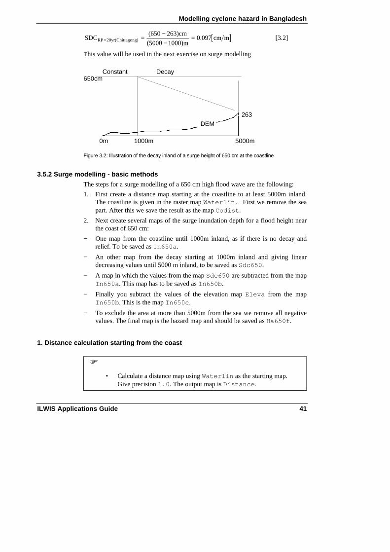
This value will be used in the next exercise on surge modelling

DEM

0m 1000m 5000m

262m262cm262cm

650cmConstant Decay

263

Figure 3.2: Illustration of the decay inland of a surge height of 650 cm at the coastline

3.5.2 Surge modelling - basic methods

The steps for a surge modelling of a 650 cm high flood wave are the following:

1. First create a distance map starting at the coastline to at least 5000m inland.The coastline is given in the raster map Waterlin. First we remove the seapart. After this we save the result as the map Codist.

2. Next create several maps of the surge inundation depth for a flood height nearthe coast of 650 cm:

− One map from the coastline until 1000m inland, as if there is no decay andrelief. To be saved as In650a.

− An other map from the decay starting at 1000m inland and giving lineardecreasing values until 5000 m inland, to be saved as Sdc650.

− A map in which the values from the map Sdc650 are subtracted from the mapIn650a. This map has to be saved as In650b.

− Finally you subtract the values of the elevation map Eleva from the mapIn650b. This is the map In650c.

− To exclude the area at more than 5000m from the sea we remove all negativevalues. The final map is the hazard map and should be saved as Ha650f.

1. Distance calculation starting from the coast

F • Calculate a distance map using Waterlin as the starting map.

Give precision 1.0. The output map is Distance.



• Display the result and check the image values.The distance calculations are also performed in the direction of thesea. Exclude the sea with the formula:

Codist:=iff(Landform=”Sea”,0,Distance)↵

2. Calculation of surge inundation depth (flood height near the coast 650 cm)

F • Type the following MapCalc formula in the command line to make

the inundation map until 5000 m from the coast for a coastal floodheight of 650 cm as if there were no decay and no relief:

In650a:=iff(Codist<=5000,650,0)↵

Save the map with domain Value and precision 1.0. Check thevalues.

• Make a map of the decay from 1000 until 5000 from the coast. Typethe formula:

Sdc650:=0.097*(Codist-1000)↵

The formula describes that for each meter distance from the coast(starting after 1000m) the map will be reduced by the Surge DecayCoefficient (SDC). Save the map with domain Value andprecision: 1.0. Check all the values.

• Subtract the pixel values of the Sdc650 map from the pixel valuesof the In650a map. Make the resulting map In650b with domainValue and check the pixel values.

• • Subtract the elevation map from In650b. Save the map as In650cwith domain Value and check the pixel values. As you will see, somepixels in the east have a negative value.

• • Finally exclude the negative values in In650c, which make no sensefor further calculations. The final hazard map is:

Ha650f:=iff(In650c<=0,0,In650c)↵

• Display the map and check the pixel values. Close the map.



3.5.3 Surge hazard modelling with an ILWIS script

In this exercise you will make several hazard maps per return period. In the mapsyou include per return period both the extend of the flooded area and the floodheight per pixel (magnitude of the hazard) .

The procedure is as follows:

a. For each recurrence interval the corresponding Surge Decay Coefficient has tobe calculated using the data from the tables 3.1 and 3.2. Do not include thetidal influence in the calculations.

b. Flood Hazard maps per return period have to be made. This can be donerelatively fast by using the ILWIS script option. With a script you make asequenced list of ILWIS operations, equivalent to a batch file. In the scriptdialogue box, type your lines of calculations and operations. The parameters ina script must be written as %1, %2, %3, etc. The script can be run from thecommand line in the main window.

c. Name the final hazard map Harety (ret = return period).

a. Calculation of the Surge Decay Coefficient interval (Chittagong zone)

Example: Return period 5 years. Corresponding surge height: 370 cm.

F • Calculate SDC for all return periods using the formula 3.1.

First you have to fill in all data in the table below using theinformation from the tables 3.1 and 3.2.

• After this, you estimate the average elevation at the end of the areaunder surge by:

First making a map of the elevations at the total surge distance fromthe coast using the maps Codist and Eleva (or DEM).Example MapCalc for the elevations at approx. 2000m from thecoast (strip of 5m wide):

Elev370:=iff((Codist>=2000)and(Codist<=2005),Eleva,0)↵

• • Next display the histogram of this map in a tabular form and makewith TabCalc an extra column with average values using theaverage function Average.

We exclude all the terrain above the surge height near the coast:

Elev:=iff(Value<=370,Value,?)↵

Avgelev:=avg(Elev)↵



• Calculate the value of SDC using the pocket line calculator and theexisting function SDC. Write the result manually in table 3.3

• Repeat this for the other maps; fill in the table below.

Table 3.3: Table to be completed manually

Return period

Surge height Chittagong (cm)

Area under const. Surge (m)

Inundated area (m)

Avg. elev. at end of surge (cm)

SDC (cm/m)

5 yr. 370 415 2000 278 0.058

10 yr.

20 yr.

50 yr.

b. Flood hazard mapping per recurrence interval using ILWIS script

F • Open the script, Surge.Study the Script file (which is printed

below). Do not change it!The Script file gives all the steps for the calculation of the surgeinundation depth (as explained in section 3.5).

• Exit the script file.

Script file

%1:=iff(Codist<=%2,%3,0)

%6:=%4*(Codist-%5)

%7:=%1-%6

%8:=%7-Eleva

%9:=iff(%8<=0,0,%8)

Explanation%1 : flood map as if there were no decay and relief (inxa.mpr) x:flood height%2 : the width of the inundated area

%3 : the flood height along the coastline (surge plus tidal height)

%4 : the value of the Surge Decay Coefficient (SDC)

%5 : the width of the area under constant surge

%6 : the map Sdcx.mpr (reduction by the SDC)

%7 : the map Inxb.mpr (x: surge height along the coast)

%8 : the map Inxc.mpr (x: surge height along the coast)

%9 : the final hazard map Harety.mpr (ret: return period of the surge height x)



Landform, Eleva, Codist: existing maps used for the calculations

F • Type in the command line of the main window the following for the

5 year return interval with a surge height along the coast of 370 cm(values from first row in the above table):

Run Surge In370a 2000 370 0.058 415 Sdc370In370b In370c Ha05y

• Meaning: run surge %1 %2 %3 %4 %5 %6 %7 %8 %9

• Hit the enter key and wait until all the calculations have beenperformed automatically. The maps In370a-c, Sdc370 andHa05y are being made.

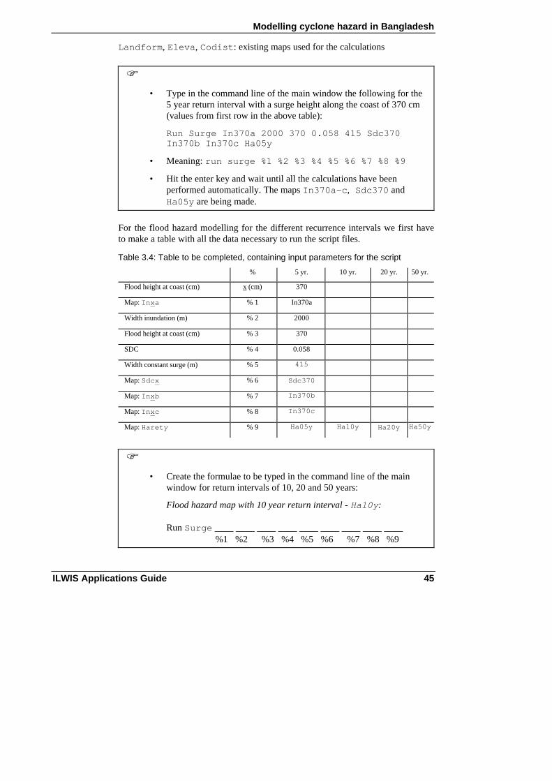
For the flood hazard modelling for the different recurrence intervals we first haveto make a table with all the data necessary to run the script files.

Table 3.4: Table to be completed, containing input parameters for the script

% 5 yr. 10 yr. 20 yr. 50 yr.

Flood height at coast (cm) x (cm) 370

Map: Inxa % 1 In370a

Width inundation (m) % 2 2000

Flood height at coast (cm) % 3 370

SDC % 4 0.058

Width constant surge (m) % 5 415

Map: Sdcx % 6 Sdc370

Map: Inxb % 7 In370b

Map: Inxc % 8 In370c

Map: Harety % 9 Ha05y Ha10y Ha20y Ha50y

F • Create the formulae to be typed in the command line of the main

window for return intervals of 10, 20 and 50 years:

Flood hazard map with 10 year return interval - Ha10y:

Run Surge ____ ____ ____ ____ ____ ____ ____ ____ ____%1 %2 %3 %4 %5 %6 %7 %8 %9




Run Surge ____ ____ ____ ____ ____ ____ ____ ____ ____%1 %2 %3 %4 %5 %6 %7 %8 %9


Run Surge ____ ____ ____ ____ ____ ____ ____ ____ ____%1 %2 %3 %4 %5 %6 %7 %8 %9

• Check the above formulae and the script file carefully.

• Type the first in the command line and press Enter. Make sure thatthere is always one space in between the parameters.

• Repeat this for the other formulae.

• Check all the hazard maps: Ha05y, Ha10y, Ha20y and Ha50y.

3.6. Vulnerability and risk analysisAfter making hazard maps per flood return interval we can also make avulnerability map of the inhabitants of the villages in the area. By calculating thepopulation density we can then estimate the number of people at risk for a certainsurge height. Finally we calculate the risk for certain categories of people, such aschildren, elderly, women and men.

3.6.1 Vulnerability analysis of the population

The vulnerability of the people to flooding is the degree of loss to the totalpopulation, or particular categories, resulting from flooding with a certain depth. Ithas to be expressed on a scale from 0 to 1.

Unfortunately we do not have sufficient good data on the vulnerability for thepeople to certain surge flood depth values. From the April 1991 cyclone in theChittagong area we know that the casualty figures in several of the villages near thecoast were as high as 70 percent of the population. In a belt at some distance fromthe coast, but still in the hazard zone, the casualty rate was in the range of 30-35percent. In the whole coastal belt, including the areas at the foot of the hills outsidethe hazard zone, deaths were probably up to 20-30 percent of the existingpopulation. The causality rates for the different population categories were asfollows: Children: 50%, Women: 25%. Elderly: 15% and Men: 10%

(Source: Cyclone 91 - An environmental and perceptional study. 1991, BangladeshCenter for Advanced Studies).

Although several warnings were given before the impact of the April 1991 cyclone,only about 16 percent of the population moved to saver places, such as a cycloneshelter or the foothills. The primary reason for staying home was fear of burglary.



The small farmers risked their lives, because they were poor and did not want totake risk of becoming even poorer.

Based on the above figures we assume the following for our calculations of thevulnerability to surge flooding of the people living in the area:

a. “Near the coast” (= 1500m) the vulnerability is 0.7. By using the inundationmap In650f and the distance map Codist we can calculate the averageflood depth at 1500 from the coast: 323 cm;

b. “At some distance from the coast” (we assume in our case = 3000m) thevulnerability is 0.3 and the average flood depth 171 cm;

c. The vulnerability function increases linear with flood depth;

d. The vulnerability of 1.0 is reached at a arbitrary depth of 450 cm

e. About 16% of the total population moved to saver places prior to the disaster.

Based on the above described assumptions the relationship between the flood depthand vulnerability is described in the table below. We have also included a columnwith the Vulnerability Coefficients (Vc). The Vc gives the increase in vulnerabilityper cm growth of the flood depth and is also an indication of the steepness of theline in the graph. The Vc of a flood depth of 0.0 cm is of course 0.000. The Vc ofthe flood depth between 0.0 and 171 cm is 0.00175, between 171 cm and 323 cm0.00217 and between 323 cm and 450 cm the highest at 0.00222. Above a flooddepth of 450 cm the Vulnerability is always 1.0. Check all this values by yourself.

By multiplying the Vc with the flood depth values of the four hazard maps Ha05y,Ha10y, Ha20y and Ha50y we will get the final vulnerability maps Vu05, Vu10,Vu20 and Vu50.

Table 3.5: Relation vulnerability and flood depth Flood depth (cm) Vulnerability Vc

0.0 0.0 0.000

171 0.3 0.00175

323 0.7 0.00217

450 1.0 0.00222

0

100

200

300

400

500

0 0.3 0.7 1

Vulerability (0 - 1)

Flo

od

dep

th (

cm)

Figure 3.3: Relation vulnerability and flood depth (see also Table 3.5)



In the next step the Vulnerability Coefficient has to be multiplied by the pixelvalues of the four hazard maps per flood depth class. At a greater depth of 450 cmthe vulnerability is always 1.

F • Use the ILWIS Script option in MapCalc to make the vulnerability

maps Vu05y, Vu10y, Vu20y and Vu50y.

• Select from the main window: File, Create, Create Script.

• Type the formula below in the Create script dialog box and give itthe name: Vulner:

%1=iff(%2=0,0,iff(%2<=171,%2*%3,iff(%2<=323,%2*%4,iff(%2<=450,%2*%5,1))))

Try to understand the syntax of this formula

• Run the script file Vulner from the command line in the mainwindow

%1: Vu05y or Vu10y, Vu20y, Vu50y%2: Ha05y or Ha10y, Ha20y, Ha50yFor all the maps: %3: 0.00175, %4: 0.00217, %5: 0.00222

• Check the values of all the vulnerability maps.

3.6.2 Calculation of the population density

In the next exercise you are going to calculate the number of people at risk pervillage. Information on the population is given in the maps and tables villageand union. In the table Village extra columns will be made with the populationdensity and population category per village. After this, a raster map will be madeusing the information from the newly made columns. For the risk analysis weassume that 16% of the population has moved to saver places prior to the cyclonedisaster (after the warning).

F • • Display the polygon map and the table Village. Rasterize the

map, if that has not yet been done.

• Use TabCalc to make extra columns of the density in hectares of thetotal population and those of children, men, women and elderlypeople.Substract first 16% of the population.

Detot:=(Popul-0.16*Popul)/(Area_m/10000)↵



Choose precision 0.01.

• Create the columns Dechild, Dewomen, Deelder, Demen.

• Now create raster maps of the population densities of the differentpopulation categories using the data in the newly made columns.The syntax of the formula to be typed in the command line of themain window is:

OutputMap:=InputMap.Table.Column

Give the output maps the same name and same precision as thecolumns in the table. The input map and table is Village. Firstcreate the output map Detot.

3.6.3 Calculation of the number of casualties per village

Example: Surge once in 50 year

To calculate the total number of casualties per village and per population categorycaused by a cyclone disaster with a certain return interval, you need the followingmaps:

a. The vulnerability maps: Vu05y, or Vu10y, Vu20y and Vu50y

b. The population density maps: Detot, Dechild, Dewomen, Deelder,Demen.

If you work in a group, do not create the maps for all the return intervals yourself.To save time, split up the work between your colleagues and let every person makethe maps for only one return interval. Compare the results. Also create sure thatthere is enough space on the hard-disk available; delete the photos or other maps, ifnecessary.

In the exercise we give an example of the calculations for a return interval of 50years. For the calculation of the number of casualties we have to multiply thevulnerability map with the population density map. However, we have to correct thevulnerability value for the individual population categories. Children for instancehave the highest vulnerability (50% of the total vulnerability of the wholepopulation) and men “only” 10%. The data are given in the table below:

Table 3.6: The vulnerability for different population categories

Population category Vulnerability %

Total 100

Children 50

Women 25

Elderly 15

Men 10



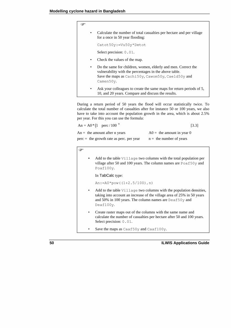
F • Calculate the number of total casualties per hectare and per village

for a once in 50 year flooding:

Catot50y:=Vu50y*Detot↵

Select precision: 0.01.

• Check the values of the map.

• Do the same for children, women, elderly and men. Correct thevulnerability with the percentages in the above table.Save the maps as Cachi50y, Cawom50y, Caeld50y andCamen50y.

• Ask your colleagues to create the same maps for return periods of 5,10, and 20 years. Compare and discuss the results.

During a return period of 50 years the flood will occur statistically twice. Tocalculate the total number of casualties after for instance 50 or 100 years, we alsohave to take into account the population growth in the area, which is about 2.5%per year. For this you can use the formula:

( )An A0 * 1 perc / 100 n= + [3.3]

An = the amount after n years A0 = the amount in year 0

perc = the growth rate as perc. per year n = the number of years

F • • Add to the table Village two columns with the total population per

village after 50 and 100 years. The column names are Poaf50y andPoaf100y.

In TabCalc type:

An:=A0*pow((1+2.5/100),n)↵

• Add to the table Village two columns with the population densities,taking into account an increase of the village area of 25% in 50 yearsand 50% in 100 years. The column names are Deaf50y andDeaf100y.

• Create raster maps out of the columns with the same name andcalculate the number of casualties per hectare after 50 and 100 years.Select precision: 0.01.

• Save the maps as Caaf50y and Caaf100y.



3.6.4 Calculation of surge flood risk in a 100 year period

The flood risk for a certain return interval is the statistical chance that peopledrown due to the surge event. It is the product of the probability of occurrence ofthe event in 100 years, the vulnerability and the number of people living in thearea. This means that the risk may change due to the frequency of the cyclones inthe future, the population growth and, for instance, the building of dikes, cycloneshelters, etc.

F • Create a map with the risk for surge flooding of the total population

in the villages per hectare for a probability of 50 years:

Riskmap:=probab.of occurrence * vulnerabilitymap * pop.density map

Save the map as Ritot50y.

• Do the same for the population categories.

• Save the maps as Richi50y, Riwom50y, Rield50y andRimen50y.

• Compare your results with the risk maps of the colleague studentswith different return intervals.

ReferencesOnly the references of the exercise are listed. At the end of the word fileappendix.doc a much longer list is given.

Cyclone 91 (1991). An environmental and perceptual study. Bangladesh Centre forAdvanced Studies.

ISPAN. (1993). GIS technology for disaster management. Contribution to theBangladesh Flood Action Plan - FAP19.

Khalil, Gazi MD. (1993). The catastrophic cyclone of April 1991: Its impact on theeconomy of Bangladesh. Natural Hazards, 8:263-281, Kluwer AcademicPublishers, The Netherlands.

Khan, S.R. (1995). Geomorphic Characterization of cyclone hazards along thecoast of Bangladesh. MSc Thesis, ITC, Enschede, The Netherlands.

MCSP. (1992). Multipurpose Cyclone Shelter Programme. Draft Final Report, Vol.IV. Planning and Development Issues, UNDP, World Bank.

Ray, S.T. (1994). An assessment of the potential of applying GIS to two aspects ofdisaster management: Storm surge modelling and cyclone shelter analysis.Msc theses, University of Nottingham, UK.



Documents

Modelling cyclone hazard in Bangladesh - ITC · Modelling cyclone hazard in Bangladesh 30 ILWIS Applications Guide 3.1 Introduction Despite the fact that the Bangladesh Government