Third draft. Please do not cite or quote without permission.

MODELLING DISTRIBUTED LAG EFFECTS IN

MORTALITY AND AIR POLLUTION STUDIES:

THE CASE OF SANTIAGO

by

David Maddison

and

Luis Cifuentes

CSERGE Working Paper

MODELLING DISTRIBUTED LAG EFFECTS IN

MORTALITY AND AIR POLLUTION STUDIES:

THE CASE OF SANTIAGO

by

David Maddison

and

Luis Cifuentes

Centre for Social and Economic Research

on the Global Environment

University College London and University of East Anglia

and

Industrial Engineering Department

Catholic University of Chile

Acknowledgements The Centre for Social and Economic Research on the Global Environment (CSERGE) is a designated research centre of the UK Economic and Social Research Council (ESRC). The authors would like to acknowledge helpful comments made on an earlier version of this paper by David Pearce. The usual disclaimer applies. ISSN 0967-8875

Abstract

Most of the epidemiological literature on air pollution and mortality deals only

with single or dual pollutant models whose results are hard to interpret and of

questionable value from the policy perspective. In addition, much of the existing

literature deals only with the very short-term effects of air pollution whereas

policy makers need to know when, whether and to what extent pollution-induced

increases in mortality counts are reversed. This involves modelling the infinite

distributed lag effects of air pollution.

Borrowing from econometrics this paper presents a method by which the infinite

distributed lag effects can be estimated parsimoniously but plausibly estimated.

The paper presents a time series study into the relationship between ambient

levels of air pollution and daily mortality counts for Santiago employing this

technique which confirms that the infinite lag effects are highly significant.

It is also shown that day to day variations in NO2 concentrations and in the

concentrations of both fine and coarse particulates are associated with short-

term variations in death rates. These findings are made in the context of a

model that simultaneously includes six different pollutants. Evidence is found

pointing to the operation of a very short term harvesting effect.

1

1. Introduction

A vast number of epidemiological studies have identified particulate matter and,

less frequently, other air pollutants as being statistically related to daily mortality

counts. Despite the fact that these studies have been undertaken in a variety of

locations the methodology followed by these studies is generally same. The

procedure is to use Poisson or Ordinary Least Squares regression analysis to

control for seasonal variations in daily mortality counts along with variations in

meteorological conditions, day-of-the-week effects, dummy variables for national

holidays and one or two pollution variables1.

Although these studies have alerted policy makers to the potential harm from

ambient pollution concentrations the results provided by time-series studies into

the mortality effects of air pollution are nonetheless turning out to be of

surprisingly limited value from the policy perspective. One problem relates to the

current emphasis on single and dual pollutant models in the epidemiological

literature. Schwartz et al (1996) remark that “One occasionally sees studies that

have fitted regression models using four or even more collinear pollutants in the

same regression… Given the non-trivial correlation of the pollutant variables and

the relatively low explanatory power of air pollution these for mortality or

hospital admissions such procedures risk letting the noise in the data choose the

pollutant”.

1 Here and elsewhere we consider only the issue of life lost due to the acute effects of air pollution. For evidence on the chronic mortality impacts of air pollution see Pope et al (1995).

2

The authors of this paper believe that alternative procedures risk allowing the

researcher to choose the pollutant. This frustrates attempts to determine which

out of a range of air pollutants are responsible for the empirically observed

mortality impacts. With the evidence as it is we cannot be certain of the extent to

which lowering particle concentrations alone, without other reducing other

combustion-related pollutants, would lower mortality. The importance to policy

makers of being able to attribute health impacts to particular pollutants should be

obvious. Policy makers have before them a range of policy and technology

options some of which entail reducing emissions of one pollutant whilst leaving

the emissions of other pollutants unchanged or even increased.

Current practice also prevents researchers from reaching any conclusions

regarding the overall health burden imposed by pollution-generating activities.

Given the non-zero correlation that often exists between different air pollutants,

reliance on the results of single pollutant models risks explaining what are

essentially the same deaths several times over. Conversely, to assume that one

pollutant such as PM10 is responsible for all of the observed health impacts risks

significantly understating the toll of air pollution on health. These problems are

avoided by multiple pollutant studies.

Matters are admittedly more complicated when one recognises ambient

concentrations recorded by monitors might be a poor representation of

individual exposure to a particular pollutant. Furthermore many pollutants

might need to be included in the same regression some of which will be

precursors of others included in the same regression. But none of these

observations justifies the almost complete reliance on single or dual pollutant

3

studies or removes the understandable need that policy makers have to be able

to attribute health impacts to particular pollutants or to calculate the overall toll

on health.

The other problem, which is in some ways the main focus of this paper, involves

the way air-pollution variables are entered into the model. Typically air pollution

is included either as a contemporaneous variable or with one or two lags.

Although such a methodology may succeed in demonstrating that air pollution

causes a short-run increase in mortality rates policy responses cannot be built

only on the basis of knowledge concerning the short-run impact of air pollution

on mortality. Policy needs to the rate at which air pollution-induced increases in

mortality counts are reversed2.

In the absence of evidence on the rate at which excess mortality counts

attributable to air pollution are reversed researchers from other disciplines have

been at a loss to know how to value such deaths from a societal point of view.

Economists for example are accustomed to valuing small changes in the risk of

mortality or even small changes in a sequence of risks in which future risks are

discounted. An air pollution episode is likely to increase the number of deaths in

the short term but lead to a reduction in the number of deaths in future time

periods. But unless they know the sequence of changes in risk or equivalently the

infinite lagged impact of air pollution on mortality economists cannot value the

air pollution episode correctly. McMichael et al (1998) provides a telling 2 Being aware of this limitation to their work typically contributors to the epidemiological literature are very careful to specify that the empirical evidence does not say anything about the extent to which life has been foreshortened as a consequence of poor air quality. Indeed

4

summary assessment of early attempts to value the mortality impacts of air

pollution.

Our paper introduces a simple modelling technique in which the entire infinite

lagged-response of daily mortality to increases in air pollution is modelled in a

plausible yet parsimonious fashion. In so doing the technique nests the kind of

models that have so far been used to explore the links between air pollution and

mortality as special cases. We argue that such methods provide a far superior

description of variations in daily mortality rates. And for the reasons given yield

insights of potentially far greater relevance to policy. This paper further provides

a demonstration of the technique using data from Santiago3.

Although the modifications to current practice presented in this paper are

intended to make the evidence offered by epidemiological research more

relevant to policy, there is no suggestion that the techniques in this paper offer

anything approaching a ‘get out of jail free’. The multicollinearity between

different pollutants makes it difficult to ascertain their individual contribution

as well as the lag effect meaning the results of individual analyses are too

uncertain to base policy. Only when the results of many different studies are

combined using meta-analytical procedures will any statistically significant

effects emerge. Rather that refraining from such ambitious studies, the point is

the epidemiological literature states in a number of places that it is impossible to measure the extent of life lost using time series studies (see for example Anderson et al 1996). 3 It should be apparent that identical issues arise in the analysis of morbidity endpoints. The Committee on the Medical Effects of Air Pollution (1998) discusses the importance of determining whether additional cases of respiratory hospital admission are caused by air pollution or whether these are simply brought forward – in which case the cost to the public should not be attributed to air pollution. The same techniques described in this paper could in principle be used answer this question.

5

that unless researchers begin to publish such studies then the data for meta-

analyses will never appear in the public domain. Meta-analysis of results

obtained from conventional studies will, of course, never answer the question

of the extent of the harvesting effect or the contribution of individual pollutants

no matter how many studies are undertaken.

The following section offers a discussion and critique of current practice in

modelling the distributed lag effects of air pollution on mortality. An alternative

method of modelling the distributed lags is introduced and the relative

advantages of the method are explained. The remainder of the paper describes the

empirical implementation of the technique within the context of a multiple

pollutant model. Section three discusses the data used to implement the model

along with the econometric modelling techniques employed. Section four

discusses the implications of the results and the final section concludes.

6

2. Modelling Lags in Time Series Air Pollution-Mortality Studies

The traditional approach to the statistical modelling of the relationship between

daily mortality counts and ambient levels of air pollution is to include just

contemporaneous, once or twice-lagged values for air pollution into a regression

equation. In these cases the choice about which lag to select is seldom explained

in detail but often it appears that the single most significant lag is chosen as for

example in Katsouyanni et al (1996).

It is however improbable that the researchers who present such models in the

literature intend them to be taken literally. For example, a researcher who seeks

to explain variations in daily mortality rates by the value of a pollutant once

lagged is not claiming that the totality of the effect is experienced precisely one

day afterwards. Nevertheless what such investigators actually end up estimating

is the ‘transient’ impact of air pollution. An extension of this approach would be

to estimate the model using single lagged-values for air pollutants ever more

distant in time. In this way one might suppose that the lagged impacts of air

pollution on mortality would emerge if the results were plotted on a graph. The

problem with this approach is that, to the extent that pollutant variables are auto-

correlated over time, the effects of adjacent lag terms will also be picked up.

Regression on a moving average of air pollution levels is perhaps a small

improvement on including just single lags (e.g. Schwartz 1994). But since it

impels the lagged effects of pollutants to be exactly equal on consecutive days

and thereafter constrains them to be zero it cannot be very realistic. In other

papers researchers estimate the coefficients on two or more consecutive

7

pollution-levels and present the cumulated impact of air pollution (e.g. Dab et al

1996). These represent a further improvement but once again require that the

impact of air pollution on mortality is zero after two or three days. A more

realistic model would allow for the lagged effects of pollutants gradually to

decay and perhaps turn negative if the deaths of susceptible individuals were

being brought forward.

In theory the means to explore such a possibility would be to estimate a model

containing many lagged terms for each of the pollutants. In practice however

analysts have avoided adding a large number of additional regressor variables to

their models. They quite rightly claim that estimation of the unrestricted

regression will not be able to locate the lag structure because it will be beset by

multicollinearity between the lagged regressors.

These reflections on current practice raise the following questions. First, how

can a distributed lag structure be modelled parsimoniously in the context of air

pollution-mortality studies (or indeed any study)? Secondly, how sensitive are

the estimated relative risk ratios to seemingly arbitrary decisions regarding the

period of time over which to cumulate the lagged impacts of air pollution?

Thirdly, to what extent can adding a more realistic lag structure reduce the

unexplained variance in a model?

A number of techniques to approximate lag structures have been proposed in

econometrics and these may be helpful in the context of epidemiological

studies too. This is a view shared by Schwartz et al (1996) who argue that the

epidemiological literature needs to pay greater heed to econometric approaches

8

to modelling distributed lags. It is also plausible that a more systematic

approach to specifying lags would allow better comparison between sites.

However, the main reason for being interested in modelling distributed lags is

in order to shed light on the question of the amount of life lost per case of

premature mortality.

One method of estimating lagged impacts is the polynomial approach of Almon

(1965). The technique involves making the assumption that the distribution of

lag coefficients can be represented by a polynomial of suitably high order. The

coefficients of the polynomial are estimated absorbing the order of the

polynomial plus one degrees of freedom.

In one of the first epidemiological studies to take advantage of this technique,

Schwartz (2000) employs a quadratic polynomial lag with a maximum lag of five

days in an analysis of the link between ambient concentrations of particulate

matter and the deaths of over-65s based on United States data4. He finds that the

use of the technique increases the measured relative risk ratios associated with

particulate matter compared to those associated with a one-day lag or a two-day

moving average. Schwartz argues that this method should become standard

practice in the epidemiological time-series studies. For a number of reasons we

do not agree with this view. The method of polynomial lags suffers from the handicap that it is necessary to

specify a finite endpoint prior to estimation. There has, in the econometrics

literature, been an extensive analysis of the consequences of miss-specifying

4 Ostro et al (1996) fit a polynomial distributed lag over the period t = 0-3 to their analysis of daily mortality counts in Santiago but provide no further details.

9

the lag length (as well as the order of the polynomial; see for example Hendry

et al 1984). Simply assuming a maximum lag length is hazardous as the Almon

lags technique will genially distribute the effects over the entire lag whether

this is appropriate or not5. Finally, the technique has extreme difficulty in

capturing any long-tailed lag distribution of the type that might well be

expected in epidemiological time-series studies (see for example Maddala

1977).

In the opinion of the authors these features serve to make the polynomial lags

technique unsuitable for use in epidemiological time-series studies. Partly

because of these shortcomings the polynomial lags technique has seen relatively

few recent applications in the field of applied econometrics. Most

econometricians take recourse in the method of ‘rational lags’ (Jorgenson, 1966)

in situations in which the modelling of distributed lags is required.

The idea behind rational lags is that any infinite distributed lag function can be

approximated by the ratio of two finite polynomials in the lag operator and as

such the rational lags technique involves only the inclusion of additional

explanatory variables. The lag operator L is defined by LXt = Xt-1. The lag

operator may be applied more than once so that L2Xt = Xt-2. It may also be

handled algebraically like an ordinary variable such that L1L2Xt = Xt-3. Consider

now the following infinite distributed lag model:

5 The Schwartz (2000) study might be criticised for simply assuming a maximum lag of five days and the appropriateness of a polynomial of degree two. There are protocols for selecting the appropriate lag lengths and order of the polynomial but these do not appear to have been followed.

10

t

i

iit

iit eXLY ++= �

∞=

=−

0βα

Rather than estimating the unrestricted model Jorgenson’s Rational Lag

technique involves estimating the following equation by means of non-linear

least squares:

tt

kktt

tj

jttt e

XLXLLXXLXLLX

Y +++++++++

+=ωωωγγγγ

α�

�

221

2210

1

It is possible to retrieve the implied parameters of distributed lag function in a

relatively straightforward manner enabling the analyst to observe the lagged

impact of a pulse change in the independent variable. Given the equivalence

between the parameters of the distributed lag and the parameters of the rational

lag function one can rewrite the equation in the following way:

( )( ) ( )33

2210

33

221

33

2210 1 LLLLLLLL γγγγωωωββββ +++=+++++++ �

By comparing coefficients of the various powers of L one obtains the following:

00 γβ =

1011 ωβγβ −=

112022 ωβωβγβ −−=

12213033 ωβωβωβγβ −−−=

1322314 ωβωβωββ −−−=

11

Notice that after the fourth term the series follows the simple recursion:

112233 ωβωβωββ −−− −−−= kkkk

These equations may now be solved recursively for each β.

The rational lag technique seems well suited to dealing with issues that arise in

epidemiological time-series studies. But to the best knowledge of the authors this

is first occasion on which its use has been seriously proposed in such a context.

Schwarz et al (1996) does however suggest the use of a geometric lag for use in

air pollution studies. Such a lag function is in fact the simplest possible example

of a rational lag formulation. The use of the geometric lag is however deeply

unappealing in this context since it assumes that the lag coefficients decline

monotonically. We have argued that a more reasonable formulation would allow

the lag coefficients to first increase and then decrease perhaps becoming negative

if the deaths of vulnerable people are being brought forward. In the next section

we illustrate the use of the technique of rational lags using data from Santiago.

12

3. The Empirical Analysis

Santiago is a city with very high levels of particulate air pollution, related in

part to its geographic situation and climatic conditions. One study showing the

relationship between levels of particulate air pollution and mortality in Santiago

has already been published (Ostro et al 1996). Using a single pollutant model

this paper shows a strong association between PM10 and daily deaths.

Daily data on non-accidental (ICD9 ≥ 800) mortality for all ages was taken from

the metropolitan area of Santiago from the start of 1988 to the end of 1996 – a

period of some 3,288 days6. Air pollution and temperature data were obtained

from the records of the urban air pollution monitoring-network. From 1988 to

1996 this network operated five monitoring stations. Four of the monitors are

closely located around downtown Santiago, and the fifth is in the far northeast

of the city. Twenty-four hour averages were obtained for PM2.5, PM10, SO2,

NO2, CO and O3 concentrations from all five stations. Measures of mean

temperature were obtained from four of the five monitoring stations. The data

are described in tables 1 and 2. Note that some missing observations have been

completed using first order regression techniques (see Maddala, 1977).

6 The metropolitan area of Santiago includes 34 municipalities but only 32 of them were included in the analysis. Two were excluded for being mostly rural with low air pollution levels. Deaths of residents of Santiago that occurred outside of Santiago were also excluded.

13

Table 1: Descriptive Statistics

Variables Mean Std.

Deviation

Minimum Maximum

MORT 56.6 12.4 22.0 116.0

TEMP (°C) 15.9 4.8 4.0 27.0

PM2.5 (µg/m3) 57.2 40.5 7.0 341.0

PM10 (µg/m3) 102.4 52.3 16.0 438.0

CO (ppb) 2.5 1.8 0.2 12.8

SO2 (ppb) 18.0 12.3 1.0 87.0

NO2 (ppb) 41.0 26.7 9.0 299.0

O3 (ppb) 90.2 63.0 3.0 963.0 Source: See text.

14

Table 2: The Correlation Matrix

MORT TEMP PM2.5 PM10 CO SO2 NO2 O3

MORT

TEMP -0.52

PM2.5 0.46 -0.51

PM10 0.41 -0.38 0.96

CO 0.50 -0.49 0.82 0.81

SO2 0.24 -0.26 0.65 0.65 0.56

NO2 0.40 -0.26 0.62 0.70 0.64 0.45

O3 -0.22 0.46 -0.04 0.03 -0.05 0.21 0.04 Source: See text.

15

The following regression equation was estimated in which L is the lag operator

and µt represents the combined influence of cyclical components and the

autonomous trend7:

This equation employs the rational lag technique to approximate an infinite

distributed-lag on both the temperature and the pollution variables. Note that

choosing i = 0-3 for both the numerator and denominator one is able to capture

quite complicated lag patterns. Choosing i = 0-3 also has the advantage of

encompassing the finite lag models typically encountered in epidemiological

research (e.g. Katsouyanni et al, 1996). Note that the same parameters ω1, ω2

and ω3 appear in the denominator of each term. This is sufficient to generate

7 The cyclical components and autonomous trends are the fitted values obtained by regressing the log of mortality on six dummy variables for different days of the week; a dummy variable for national holidays; a cubic time trend and sine and cosine terms of various frequencies. The coefficients on the sine and cosine terms were allowed to vary over the years. In this way the presence or absence of epidemics and changes in the timing of the seasonal peak and the size of the seasonal peak to trough ratio were accounted for.

t

t

i

i

ii

t

i

i

ii

i

it

ii

t

i

i

ii

i

it

ii

t

i

i

ii

t

i

i

ii

t

i

i

ii

t

i

i

ii

t

i

i

ii

t

i

i

ii

t

i

i

ii

t

i

i

ii

t

i

i

ii

t

i

i

ii

t

i

i

ii

tt

eOL

OL

NOL

ONL

SOL

SOL

COL

COL

PML

PML

PML

PML

TEMPL

TEMPL

TEMPL

TEMPL + = MORT

++

++

++

++

++

++

++

++

−

�

�

�

�

�

�

�

�

�

�

�

�

�

�

�

�

=

=

=

=

=

=

=

==

=

=

==

=

=

=

−

=

=

−

=

=

=

=

=

==

=

=

==

=

=

=

3

3

1

3

3

0

3

12

2

3

03

12

2

3

0

2

3

1

2

3

0

5.210

3

1

5.210

3

0

5.2

3

1

5.2

3

0

23

1

23

03

1

3

0

1

1111

111)log(

ω

δ

ω

ρ

ω

θ

ω

ν

ω

σ

ω

λ

ω

ψ

ω

γαµ

16

infinite lagged effects for every variable but an even more flexible model would

allow them to vary.

The influence of temperature on mortality is well documented. The association

is not linear, with some studies reporting a U-shaped relationship. We

accommodate this by including a quadratic term for temperature with the mean

subtracted. Rather than include PM10 and PM2.5 as separate regressors we

include PM2.5 (fine particles) and PM10-2.5 (coarse particles) in an attempt to

reduce the level of multicollineary between these regressors.

The error term was assumed to be normally identically and independently-

distributed and estimates of the parameters were obtained by using maximum

likelihood estimation techniques8. Examination of the residuals yields no

evidence of autocorrelation (the Durbin-Watson statistic is 2.02). This also

suggests that the cyclical components and autonomous trends have been

satisfactorily controlled for. The R2 statistic was 0.04. Full details of the

estimation results are available from the authors on request.

8 In many empirical analyses the error term is assumed to be a Poisson variable. In this analysis the daily number of deaths is typically very large and there is probably no discernible difference from modelling the error term as a Normal variable.

17

4. Discussion

The main point of interest is whether the exclusion of those additional terms that

allow for infinite lagged impacts represents a statistically significant loss of fit.

The alternative is a model, like those currently encountered in the literature, in

which the effects of air pollution and meteorological variables can be

satisfactorily represented by allowing for only three lagged terms. A likelihood-

ratio test suggests that the loss of fit from setting parameters ω1, ω2 and ω3

equal to zero is significant at the one-percent level9. This finding provides

strong support for the use of the rational-lags technique in the context of air

pollution mortality studies.

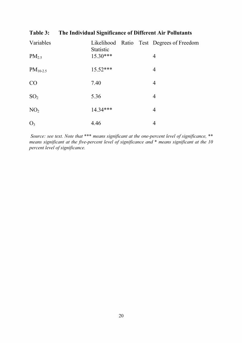
Turning to the question of whether individual air pollutants are statistically

significant or not, the results of a suite of likelihood ratio tests are presented in

table 3. This table suggests that when tested against a model containing all six

air-pollutants three out of six air pollutants are statistically significant at the one-

percent level of significance. The remaining air pollutants are not statistically

significant even at the ten-percent level of significance. Beyond this it is difficult

to compare these results to the existing literature. First and foremost this is

because most researchers are measuring either the transient impact of air

pollution at variety of lag lengths or the interim impact cumulated over an

arbitrary number of days. The rational-lags technique by contrast calculates a

different transient impact at each lag length. Secondly, unlike most other

9 The χ2 Statistic is 11.56 against a critical value of 11.34 at the one-percent level of significance with 3 degrees of freedom.

18

analyses, this study calculates the mortality effects of air pollution within the

context of a multiple pollutant rather than a single pollutant model.

Table 4 presents the lag coefficients cumulated over different lag lengths. The

first observation is that the lag coefficients cumulated over t = 0-7 differ from

the coefficients at time t = 0. More specifically they are reduced not only in

terms of their significance but also in terms of their absolute value. Furthermore

the cumulative lag coefficients do not appear to change even to two significant

figures when cumulated over periods between t = 0-7 and t = 0-∞. This is

evidence consistent with the existence of a very short term harvesting effect.

Note that the cumulated coefficients over the period t = 0-∞ are not restricted to

sum to zero even though common sense suggests that this restriction should hold.

In fact, although it is easy to restrict the model such that the lag coefficients

cumulated over the period t = 0-∞ sum to zero we prefer to test the hypothesis

using a Wald test. The hypothesis is not rejected even at the 10 percent level of

significance10. We do not however recommend imposing this restriction as a

matter of course since it might sometimes interfere with the ability of the model

to represent short-term lags.

There are a number of other interesting points that emerge from the current

analysis. The first is that whereas the majority of attention has been focussed on

particulate matter, an increased concentration of NO2 is also seen to result in a

significant variation in short term mortality rates. Other researchers have also 10 The statistic is 9.92 against a critical value of 10.64 at the ten-percent level of significance with 6 degrees of freedom.

19

identified NO2 as a significant cause of premature mortality: for a survey and

meta-analysis see Touloumi et al (1997). Secondly, whilst CO is associated

with a significant effect at lag t = 0 according to the Likelihood Ratio test CO is

statistically insignificant. As an empirical matter it is not unusual for a Wald

test and a Likelihood Ratio test to give different results although here the

difference is quite pronounced.

Finally, even though they are to some extent collinear it nonetheless appears

useful to distinguish between fine particles and coarse particles. More

specifically it appears that whereas fine particles are significantly associated

with short term increases in mortality, coarse particles are associated with a

significant reduction in short term mortality. One interpretation might be that

whilst fine particulate matter is harmful to health coarse particulate matter is

not. Furthermore the fact that coarse particulate matter has a negative

coefficient might indicate that only very fine particulate matter is an important

cause of premature mortality.

20

Table 3: The Individual Significance of Different Air Pollutants

Variables Likelihood Ratio Test Statistic

Degrees of Freedom

PM2.5

15.30*** 4

PM10-2.5

15.52*** 4

CO

7.40 4

SO2

5.36 4

NO2

14.34*** 4

O3

4.46 4

Source: see text. Note that *** means significant at the one-percent level of significance, ** means significant at the five-percent level of significance and * means significant at the 10 percent level of significance.

21

Table 4: Air Pollution as an Influence on Mortality Rates (All Ages)

Variables Cumulated Over t = 0

Cumulated Over t = 0-7

Cumulated Over t = 0-∞

PM2.5

0.35E-03** (0.14E-03)

-0.13E-03 (0.16E-03)

-0.13E-03 (0.16E-03)

PM10-2.5

-0.64E-03*** (0.25E-03)

-0.26E-03 (0.30E-03)

-0.26E-03 (0.30E-03)

CO

0.62E-02** (0.31E-02)

0.51E-02 (0.32E-02)

0.51E-02 (0.32E-02)

SO2

0.22E-03 (0.38E-03)

0.11E-03 (0.31E-03)

0.11E-03 (0.31E-03)

NO2

-0.35E-03** (0.17E-03)

0.30E-03* (0.18E-03)

0.30E-03* (0.18E-03)

O3

0.38E-05 (0.23E-04)

0.11E-03 (0.86E-04)

0.11E-03 (0.86E-04)

Source: see text. Figures relate to the estimated lag coefficients. Standard errors are in parentheses and have been calculated using the delta method. Note that *** means significant at the one-percent level of significance, ** means significant at the five-percent level of significance and * means significant at the 10 percent level of significance.

22

5. Conclusions

This paper has noted the problem of interpretation that the use of single pollutant

models presents policy makers. The simple solution is for epidemiologists to

present the results of multiple pollutant models and for policy makers to base

their results exclusively upon them.

This paper has also noted that much of the existing epidemiological literature

estimates only the very short-term transient or cumulative impacts of air

pollution. But cumulating the impacts of air pollution over the very short term

or presenting only the transient impacts at lags t = 0 or t = 1 could inadvertently

give policy-makers or those from other disciplines a misleading impression of

the health risks posed by the acute effects of air pollution. The most probable

reason for the focus on the very short-term impacts is that epidemiologists have

hitherto not known how to model infinite lags in a parsimonious manner.

Noting the deficiencies of alternative techniques, this paper has used the method

of rational lags to approximate the infinite distributed lag impact of a change in

air pollution. The method is straightforward and involves including additional

terms that permit one to approximate the entire distributed lag. In the case of

Santiago these are shown to dramatically improve the fit of the regression

equation even in the context of a multiple pollutant model.

Because the results from any one study are too uncertain to be used as a basis for

policy it would be interesting to reanalyse the data from existing studies using

this technique. By computing the cumulated impact of air pollution at fixed

23

intervals (e.g. up to one day, one week and one month) and combining the results

it may be possible to determine the speed with which excess mortality attributed

to the acute impacts of air pollution is reversed. The standard errors of the

parameters of interest in this study suggest that large numbers of studies would

be required in order for statistically significant results to emerge. Fortunately

there are many data sets available for analysis. But in order to be meaningful

such comparisons must be careful to compare the impacts cumulated over

identical periods of time and, if they intend to be policy relevant, should certainly

avoid focussing solely on the very short-term impacts.

24

References

Almon, S. (1965) The Distributed Lag between Capital Appropriations and

Expenditures Econometrica Vol. 33 pp178-196.

Anderson, H., A. Ponce de Leon, J. Bland, J. Bower and D. Strachan (1996) Air

pollution and daily mortality in London: 1987-92. British Medical Journal

Vol. 312 pp665-669.

Committee on the Medical Effects of Air Pollution (1998) Quantification of the

Effects of Air Pollution on Health in the United Kingdom. London:

HMSO.

Dab, W., S. Medina, P. Quenel, Y. Le Moullec, A. Le Tertre, B. Thelot, C.

Monteil, P. Lameloise, P. Pirard, I. Momas, R. Ferry and B. Festy (1996)

Effects of Ambient Air Pollution in Paris. Journal of Epidemiology and

Community Health Vol. 50 (Supp.) pp42-46.

Hendry, D. Pagan A. and Sargan, J. (1984) Dynamic Specifications. In Griliches,

Z. and Intriligator, I. Handbook of Econometrics Vol. 2, North Holland:

Amsterdam.

Jorgenson, D. (1966) Rational Distributed Lag Functions. Econometrica, Vol. 34

pp135-149.

25

Katsouyanni, K., J. Schwartz, C. Spix, G. Touloumi, D. Zmirou, A. Zanobetti, B.

Wojtyniak, J. Vonk, A. Tobias, A. Ponka, S. Medina, L. Bacharova and H.

Anderson (1996) Short Term Effects of Air Pollution on Health: A

European Approach Using Epidemiologic Time Series Data: The APHEA

Protocol Journal of Epidemiology and Community Health Vol. 50 (Supp.)

pp12-18.

McMichael, A., H. Anderson, B. Brunekreef and A. Cohen (1998) Inappropriate

Use of Daily Mortality Analyses to Estimate Longer-Term Mortality

Effects of Air Pollution. International Journal of Epidemiology Vol. 27

pp450-453.

Maddala, G. (1977) Econometrics McGraw-Hill: Singapore.

Ostro, B., J. Sanchez, C. Aranda and G. Eskeland (1996) Air Pollution and

Mortality: Results from a Study of Santiago, Chile. Journal of Exposure

Analysis and Environmental Epidemiology Vol. 6, pp97-114.

Pope, C., M. Thun, M. Namboodiri, D. Dockery, J. Evans, F. Speizer and C.

Heath (1995) Particulate Air Pollution as a Predictor of Mortality in a

Prospective Study of US Adults. American Journal of Respiratory and

Critical Care Medicine Vol. 151 pp669-674.

Schwarz, J. (1994) Total Suspended Particulate Matter and Daily Mortality in

Cincinnati, Ohio. Environmental Health Perspectives Vol. 102 No. 2

pp186-189.

26

Schwarz, J. (2000) The Distributed Lag between Air Pollution and Daily Deaths.

Epidemiology Vol. 11 No. 3 pp320-326.

Schwarz, J. and D. Dockery (1992) Increased Mortality in Philadelphia

Associated with Daily Air Pollution Concentration. American Review of

Respiratory Disease Vol. 145 pp600-604.

Schwarz, J., C. Spix, G. Touloumi, L. Bacharova, T. Barumamdzadeh, A. Le

Tertre, T. Piekarski, A. Ponce De Leon, A. Ponka, G. Rossi, M. Saez, and

J. Schouten (1996) Methodological Issues in Studies of Air Pollution and

Daily Counts of Deaths or Hospital Admissions. Journal of Epidemiology

and Community Health Vol. 50 (Supp.) pp3-11.

Touloumi, G., K. Katsouyanni, D. Zmirou, J. Schwartz, C. Spix, A. Ponce de

Leon, A. Tobias, P. Quennel, D. Rabczenko, L. Bacharova, L. Bisanti, J.

Vonk and A. Ponka (1997) Short Term Effects of Ambient Oxidant

Exposure on Mortality: A Combined Analysis Within the APHEA Project.

American Journal of Epidemiology Vol. 146 pp177-185.