Modelling Firebreaks in a Two-Dimensional Dynamic Fire

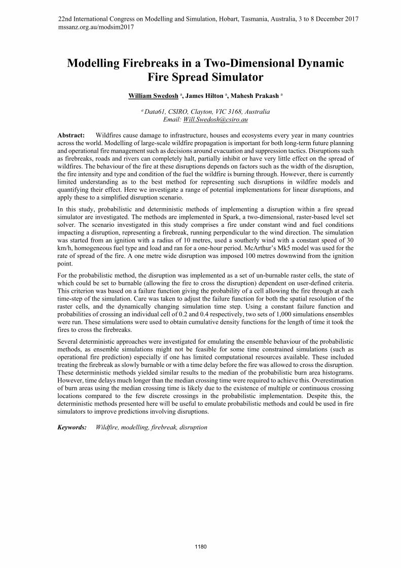
Modelling Firebreaks in a Two-Dimensional Dynamic Fire Spread Simulator

William Swedosh a, James Hilton a, Mahesh Prakash a

a Data61, CSIRO, Clayton, VIC 3168, Australia Email: [email protected]

Abstract: Wildfires cause damage to infrastructure, houses and ecosystems every year in many countries across the world. Modelling of large-scale wildfire propagation is important for both long-term future planning and operational fire management such as decisions around evacuation and suppression tactics. Disruptions such as firebreaks, roads and rivers can completely halt, partially inhibit or have very little effect on the spread of wildfires. The behaviour of the fire at these disruptions depends on factors such as the width of the disruption, the fire intensity and type and condition of the fuel the wildfire is burning through. However, there is currently limited understanding as to the best method for representing such disruptions in wildfire models and quantifying their effect. Here we investigate a range of potential implementations for linear disruptions, and apply these to a simplified disruption scenario.

In this study, probabilistic and deterministic methods of implementing a disruption within a fire spread simulator are investigated. The methods are implemented in Spark, a two-dimensional, raster-based level set solver. The scenario investigated in this study comprises a fire under constant wind and fuel conditions impacting a disruption, representing a firebreak, running perpendicular to the wind direction. The simulation was started from an ignition with a radius of 10 metres, used a southerly wind with a constant speed of 30 km/h, homogeneous fuel type and load and ran for a one-hour period. McArthur’s Mk5 model was used for the rate of spread of the fire. A one metre wide disruption was imposed 100 metres downwind from the ignition point.

For the probabilistic method, the disruption was implemented as a set of un-burnable raster cells, the state of which could be set to burnable (allowing the fire to cross the disruption) dependent on user-defined criteria. This criterion was based on a failure function giving the probability of a cell allowing the fire through at each time-step of the simulation. Care was taken to adjust the failure function for both the spatial resolution of the raster cells, and the dynamically changing simulation time step. Using a constant failure function and probabilities of crossing an individual cell of 0.2 and 0.4 respectively, two sets of 1,000 simulations ensembles were run. These simulations were used to obtain cumulative density functions for the length of time it took the fires to cross the firebreaks.

Several deterministic approaches were investigated for emulating the ensemble behaviour of the probabilistic methods, as ensemble simulations might not be feasible for some time constrained simulations (such as operational fire prediction) especially if one has limited computational resources available. These included treating the firebreak as slowly burnable or with a time delay before the fire was allowed to cross the disruption. These deterministic methods yielded similar results to the median of the probabilistic burn area histograms. However, time delays much longer than the median crossing time were required to achieve this. Overestimation of burn areas using the median crossing time is likely due to the existence of multiple or continuous crossing locations compared to the few discrete crossings in the probabilistic implementation. Despite this, the deterministic methods presented here will be useful to emulate probabilistic methods and could be used in fire simulators to improve predictions involving disruptions.

Keywords: Wildfire, modelling, firebreak, disruption

22nd International Congress on Modelling and Simulation, Hobart, Tasmania, Australia, 3 to 8 December 2017 mssanz.org.au/modsim2017

1180

Swedosh et al., Modelling Firebreaks in a Two Dimensional Dynamic Fire Spread Simulator

1. INTRODUCTION

Accurate modelling of large-scale wildfires is necessary for both long-term risk assessment and operational fire management. Whilst operational predictive models are aimed at capturing the effect of wind, fuel and topography on fire spread, the understanding and incorporation of disruptions in the landscape such as firebreaks, roads and rivers are less understood. Developing and implementing models which capture the effect of these disruptions on the spread of fires in the landscape may lead to more accurate predictions of fire spread.

Disruptions can either stop or have little effect on the spread of wildfires. Studies have shown that the probability of fires crossing firebreaks depends on factors such as the fire intensity, the width of the disruption and type and condition of the fuel the wildfire is burning through (Wilson 1988). Detailed computational fluid dynamics (CFD) models have shown that whether a fire crosses a firebreak or not depends on the width of the disruption, the adjacent fuel characteristics, the local slope of the terrain and the local meteorological conditions (Bellemare et al., 2007 and Morvan, 2015). A key finding in these numerical studies was that radiation from the fire plays a large role in whether the fire crosses the firebreak and continues propagating on the other side. However, the detailed inputs and the computational time required to run such models mean they are unlikely to be used in operational wildfire models in the near future. Wilson (1988) carried out experiments in which grass plots of 100m by 100m were set alight and allowed to burn up to firebreaks of various widths. The findings from these experiments were developed into empirical relationships which, due to their relative simplicity, could be incorporated into operational wildfire models. However, there is currently limited understanding of the best method for implementing these relationships in a predictive fire model.

In this study, we use a two-dimensional dynamic fire spread simulator to implement both probabilistic and deterministic methods of firebreak crossings for a simple fire spread scenario. The probabilistic methods rely on stopping the fire progression at a disruption and testing against a failure function giving the probability of the fire crossing the disruption. The mechanism of fire crossing being simulated is by flame contact and radiation, rather than spotting where flaming embers are lofted above the surface fuel. Ensemble simulations using the probabilistic method are carried out to assess the median influence of the disruption on the fire progression. In some instances, ensemble simulations may not be able to be used due to the need for a large simulation set, requiring significant computational time. Hence, we also use the ensemble results to develop and test deterministic methods which emulate the median behaviour of the probabilistic methods, but require only a single simulation. The probabilistic and deterministic disruption methods presented in this study could be used in operational models in the future to improve fire prediction when disruptions are present. The methods and results are presented and discussed in the following sections.

2. METHODOLOGY

In this study, Spark (Miller et al. 2015) was used to test and implement various firebreak crossing methodologies. Spark is a two-dimensional, raster based level set solver with the capability to allow individual raster cells to be un-burnable or to burn with a user-defined rate of spread. The state can be switched from ‘burnable’ to ‘un-burnable’ or vice versa based on user-defined criteria.

A schematic diagram of the implementation for disruptions is shown in Fig. 1. At the initialisation state, all raster cells within the domain were set to the ‘burnable’ state. A check was then carried out for any cells intersecting with a disruption which were set to the ‘un-burnable’ state. Disruptions can be manually entered or imported into the model as either vector or raster layers. Here, the disruption was manually entered as a line of grids cells. For the probabilistic fire simulations, the fire perimeter was propagated and any cells within the active region near the fire were checked to see if they were in the disruption layer in an ‘un-burnable’ state. For the probabilistic crossing simulations, a random number was generated and tested against the probability of failure. If the test succeeded, the cell was marked as ‘burnable’ and the fire could spread into the cell. Once the fire had burned into previously un-burnable cells, it could propagate to the other side of the firebreak.

A straightforward set-up was used in this study for both the probabilistic and deterministic disruption crossing methods. The set-up comprised a fire starting from a circular ignition with a radius of 10 metres, with a variable wind of constant strength 30 km/h and a normal distribution in direction of width 20 degrees about the southerly direction. A homogeneous fuel type and load was applied for a simulation duration of one hour. A one metre (one grid cell) thick firebreak was imposed running perpendicular to the direction of fire spread, 100 metres downwind from the centre of the ignition point. The Noble et al. (1980) equation based on McArthur’s (1973) Mk 5 Forest Fire Danger Meter was used as the rate of spread for all simulations. The set-up is shown in Fig. 2, where the colours in the image represent arrival time of the fire at each location. The fire spreads in a northerly direction until stopped at the fire break (horizontal blue line in Fig. 2). In the example shown in this figure, no check for crossing of the firebreak occurs and the disruption completely stops the fire.

1181


Figure 1. A diagram showing a fire approaching a row of firebreak cells. Yellow cells are burning or have previously burned, blue cells are currently un-burnable, green cells are being checked to see whether they become burnable or not.

Figure 2. Plan view of a wildfire simulation where the disruption

(horizontal blue line) stops the fire spread. Colour shows arrival time (s).

2.1. Probabilistic Crossings

For the probabilistic crossing of the disruption, a failure function was tested at every cell of the disruption once the fire was in close proximity. For example, a constant failure function assumes that the fire has a constant intensity and flame length while the fuel is burning. A random number was generated from a uniform distribution using the MWC64X OpenCL random number generator1 with a given random seed and tested against the probability from the failure function to determine whether the firebreak failed in that particular grid cell or not. Multiple simulations were performed, each one with a different random seed. Any given simulation from this ensemble could result in the fire either not crossing the disruption at all or crossing the disruption in one or more places at different times.

Spatial resolution considerations To implement a cell-wise disruption methodology, the probability of a single disruption cell being breached must be carefully defined. In order to do this, empirical relationships to estimate firebreak crossing probability such as in Wilson (1998) could be used:

= , , (1)

where is fireline intensity, is firebreak width and is the presence of trees near the firebreak. These relationships have been based on experimental results in plots of grass 100m to 200m wide, thus restricting the width of the head fires approaching the firebreak. The probabilities that such empirical models give as outputs should really be treated as probabilities per length, in this case the probability of beaching the firebreak per 100 metres of fire line. Extending the probability of a firebreak failing from a 100m head fire to longer or shorter fire lines can be done using binomial theory assuming that sections of fire line are independent. We assume this independence in this study.

As Spark performs calculations on each cell within a raster, the probability of each individual cell failing is calculated independently. In order to maintain a constant failure probability per length of the firebreak, the probability of failure of an individual cell should vary with cell length as follows:

_ = 1 − 1 − / (2)

where is the cell length and is the probability of a set length of firebreak (100m) being breached.

In this study, arbitrary crossing probabilities per length are used as an example however relationships such as in Equation 2 will be input into the system in future work.

Time step considerations As the solver has an adaptive time step which decreases with increasing rate of spread, it is important that the total failure probability of the firebreak per cell is independent of the time step. As the fire would generally

1 Based on the implementation by David Thomas, available from: http://cas.ee.ic.ac.uk/people/dt10/research/rngs-gpu-mwc64x.html

1182


burn out a certain time after reaching a firebreak (assuming it doesn’t cross), for a continuous failure probability density function we would require:

_ = − (3)

where is the arrival time of the fire to the firebreak, is the amount of time taken for the vegetation next to the firebreak to burn out and − is the probability density function (continuous random variable) which defines the probability of the cell being breached once the fire arrives. The integral in Equation 3 can be simplified with the substitution ∗ = − :

_ = ∗ ∗ (4)

where ∗ is the time since the fire arrives at the firebreak. The function ∗ can take a variety of functional forms, from a constant value representing a steady probability of firebreak breach to an exponential decay function representing the decreasing heat release rate of the fuel as it burns. While the functional form of ∗ does not effect the breach probability as long as Equation 4 is satisfied, it will affect the distribution of crossing times, with a decay function weighting short crossing times more so than long crossing times.

The continuous random variable then needs to be converted into a discrete random variable as wildfire propagation solvers use discrete time steps to modify fire behaviour or propagate fire perimeters. Let us define ascending times ∗, ∗, … , ∗, … , ∗ with corresponding time steps ∆ ∗, ∆ ∗, … , ∆ ∗, … , ∆ ∗ such that ∗ = and ∆ ∗ = ∗ − ∗ . We then have:

_ _∆ ∗ = ∗∗ ∗ (5)

and for the later time steps we must use conditional probabilities as follows:

_ _∆ ∗ = ∗∗∗ ∗1 − _ _ ∗ (6)

where

_ _ ∗ = _ _∆ ∗ + _ _∆ ∗ + ⋯+ _ _∆ ∗ , ≠

which doesn’t hold true for = as _ _ ∗ = 1 when ∗ is a true probability density function (integral equals 1), ensuring that the firebreak is crossed eventually. As a consequence of this, if it is predicted that the breach probability (per length or per cell) is less than 1 (which will be common for low intensity fires or wide firebreaks), then ∗ will not be a true probability density function (unless we have instances such as non-zero values of ∗ outside the integral domain) as the integral in Equation 4 will be less than 1.

2.2. Deterministic Crossings

While running dozens or hundreds of fire spread simulations using probabilistic crossings of firebreaks can provide high fidelity results for some scenarios (perhaps such as planning a fuel reduction burn), it may not be possible or practical to implement in time-critical circumstances such as live fire prediction. As such, deterministic models may be the most appropriate to use in some situations. Some possible deterministic implementations are:

1. Treating the firebreak as a time delay to any fire which propagates to become adjacent to it. The fire would remain adjacent to the firebreak for a set period of time before it can be crossed.

2. Treating the firebreak as burnable, but with a lower rate of spread compared to the adjacent vegetation. This may be appropriate when the firebreak is a recent hazard reduction burn or recently mown grass.

3. Treating the entire firebreak as a single time delay once any part of the fire becomes adjacent to it. This is probably the least realistic when it comes to the mechanics of crossing a road or river.

1183


3. RESULTS

3.1. Probabilistic method

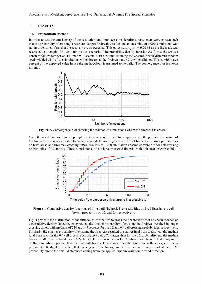
In order to test the consistency of the resolution and time step considerations, parameters were chosen such that the probability of crossing a restricted length firebreak was 0.5 and an ensemble of 1,000 simulations was run in order to confirm that the results were as expected. This gave _ = 0.0168 as the firebreak was restricted to a length of 41 cells for this test scenario. The probability density function ∗ was chosen as a constant failure rate for an assumed 900 second burn out time. Running the ensemble with different random seeds yielded 51% of the simulations which breached the firebreak and 49% which did not. This is within two percent of the expected value hence the methodology is assumed to be valid. The convergence plot is shown in Fig. 3.

Figure 3. Convergence plot showing the fraction of simulations where the firebreak is crossed.

Once the resolution and time step implementations were deemed to be appropriate, the probabilistic nature of the firebreak crossings was able to be investigated. To investigate the effect of firebreak crossing probabilities on burn areas and firebreak crossing times, two lots of 1,000 simulation ensembles were run for cell crossing probabilities of 0.2 and 0.4. These simulations did not have restricted fire widths that the test ensemble did.

Figure 4. Cumulative density functions of time until firebreak is crossed. Blue and red lines have a cell breach probability of 0.2 and 0.4 respectively.

Fig. 4 presents the distribution of the time taken for the fire to cross the firebreak once it has been reached as a cumulative density function. As expected, the smaller probability of crossing the firebreak resulted in longer crossing times, with medians of 224 and 147 seconds for the 0.2 and 0.4 cell crossing probabilities, respectively. Similarly, the smaller probability of crossing the firebreak resulted in smaller final burn areas, with the median total burn area for the 0.4 cell crossing probability being 7% larger than for the 0.2 probability and the median burn area after the firebreak being 66% larger. This is presented in Fig. 5 where it can be seen that many more of the simulations predict that the fire will burn a larger area after the firebreak with a larger crossing probability. It should be noted that the edges of the histogram before the firebreak are not all at 100% probability due to the small differences arising from the applied random variation in wind direction.

1184


a) Probability of cell breach is 0.2 b) Probability of cell breach is 0.4

Figure 5. Histograms of burn areas. Colour scale shows the percentage of simulations arriving at each cell.

3.2. Deterministic

Three deterministic implementations of firebreak crossing were simulated in order to compare the results with the probabilistic crossing results. Crossing time values for the 0.2 and 0.4 cell crossing probabilities were chosen from the cumulative density functions. Percentiles of 50, 90 and 99 were chosen as crossing time delays and the results qualitatively compared. Arrival time plots with isochrones for deterministic implementations 1, 2 and 3 are shown in Fig. 6, 7 and 8 respectively where the individual images are labelled with their cell crossing probabilities and the percentile of the time delay cumulative density function that was used.

The delayed crossing simulations (Fig. 6) result in similar burn areas to the burnable firebreak simulations (Fig. 7). The main difference is the sharp vertices at the firebreak for the delayed crossings compared to the more transitional thinning of the head fire in the burnable firebreak simulations. The simultaneous failure of the firebreak (Fig. 8) did not seem to give as close of a match to the median of the ensembles as the other methods kept the rounded near elliptical head fire rather than a more flattened linear head fire.

p = 0.2, 50th p = 0.2, 90th p = 0.2, 99th p = 0.4, 50th p = 0.4, 90th p = 0.4, 99th

Figure 6. Fire spread simulations where the firebreak is treated as a time delay for each cell. Colour shows arrival time. Black isochrones at 5 minute intervals.


Figure 7. Fire spread simulations where the firebreak is treated as slowly burnable in order to achieve a time delay. Colour shows arrival time. Black isochrones at 5 minute intervals.

1185



Figure 8. Fire spread simulations where the entire firebreak is treated as a simultaneous time delay. Colour shows arrival time. Black isochrones at 5 minute intervals.

4. DISCUSSION AND CONCLUSIONS

We have implemented probabilistic and deterministic methods for disruptions within fire propagation simulations and demonstrated that these can model disruption behaviour in a straightforward test scenario. For the probabilistic method, cumulative density functions of crossing times were created for multiple probabilities of crossing the firebreak. Lower firebreak crossing probabilities resulted in longer crossing lag times. For the deterministic method, treating the firebreak as slowly burnable or as a time delay yielded similar results to the median of the probabilistic burn area histograms. However, time delays of much longer than the median crossing time were needed to achieve this. Overestimation of burned areas using the median crossing time is likely due to multiple or continuous crossing locations compared to the few discrete crossings in the probabilistic implementation.

Ideally, such disruption models could be used for operational purposes in both planning and emergency response scenarios. The most appropriate model would depend on the use case. For example, a probabilistic disruption model may be more appropriate for developing risk profiles of a single wildfire or planned burn. If a worst-case scenario was being modelled, then it may be appropriate to ignore firebreaks entirely, treating them the same as the surrounding vegetation (possibly while giving outputs on firebreak breach probability). If a landscape scale risk assessment is being conducted then it may be most appropriate to use a deterministic method by which the median time to cross the firebreak is used.

Future work will include implementing empirical relationships which estimate firebreak crossing probabilities from firebreak width and fire line intensity. Furthermore, the current system allows us to use local fire line intensity as input into these relationships, allowing greater probability that head fire will breach firebreaks rather than flanking fires. The orientation of the firebreak with respect to the wind and fire propagation directions will also be investigated as an input into the probability of crossing firebreaks.

REFERENCES

Bellemare L.O., Porterie B., Loraud J.C. (2001). On the Prediction of Firebreak Efficiency, Combustion Science and Technology, 163, 131-176

McArthur A.G. (1973). Forest Fire Danger Meter Mark V. Commonwealth Department of National Development Forestry and Timber Bureau, Canberra, ACT.

Miller C., Hilton J., Sullivan A., Prakash M. (2015). SPARK – A Bushfire Spread Prediction Tool. ISESS 2015. IFIP Advances, vol 448. Springer, Cham

Morvan D. (2015). Numerical study of the behaviour of a surface fire propagating through a firebreak built in a Mediterranean shrub layer, Fire Safety Journal, 71, 34-48

Noble I.R., Bary G.A.V. and Gill A.M. (1980). McArthur’s fire-danger meters expressed as equations. Australian Journal of Ecology 5, 201-203.

Wilson A.A.G. (1988). Width of firebreak that is necessary to stop grass fires: some field experiments. Canadian Journal of Forest Research, 18, 682–687

1186

Documents

Modelling Firebreaks in a Two-Dimensional Dynamic Fire