Embed Size (px)
Citation preview
Modelling for the COVID-19 with the ContactingDistanceZhihui Ma ( [email protected] )
Lanzhou UniversityShufan Wang
Northwest Minzu UniversityXuanru Lin
Lanzhou UniversityXiaohua Li
Lanzhou UniversityXiaotao Han
Northwest Minzu UniversityHaoyang Wang
McMaster UniversityHua Liu
Northwest Minzu University
Research article
Keywords: COVID-19, Contacting distance, Immigration rate, Sensitivity analysis, Numerical test, Controlmethod
Posted Date: March 22nd, 2021
DOI: https://doi.org/10.21203/rs.3.rs-329034/v1
License: This work is licensed under a Creative Commons Attribution 4.0 International License. Read Full License

Zhihui Ma et al.
RESEARCH
Modelling for the COVID-19 with the contactingdistanceZhihui Ma1*, Shufan Wang2, Xuanru Lin1, Xiaohua Li1, Xiaotao Han2, Haoyang Wang3 and Hua Liu2
*Correspondence:
[email protected] of Mathematics and
Statistics, Lanzhou University,
Lanzhou,Gansu 730000, People’s
Republic of China
Full list of author information is
available at the end of the article
Abstract
Background: The COVID-19, which belongs to the family of Coronaviridae andis large-scale outbreak in the whole world, is a public health emergency forhuman beings and brings some very harmful consequences in social and economicfields. For COVID-19, the contacting distance between the healthy individualsand the asymptomatic or symptomatic infected individuals is an important factorin its spread. Therefore, the contacting distance must be considered in order tomodelling the COVID-19 and develop the efficient control method correspondingto the contacting distance,
Methods: This paper proposes an SEIR-type epidemic model and incorporatesthe contacting distance between the healthy individuals and the asymptomatic orsymptomatic infected individuals into the proposed model based on the spreadmechanism of the COVID-19. The proposed model with the contacting distanceis analysed by the methods of differential dynamical systems and the realisticmeanings are revealed. Methods:
Results: Firstly, the results show that the COVID-19 will be controlled while thecontacting distance between the healthy individuals and the symptomaticinfected individuals is larger than the threshold value d∗ and the immigration rateis smaller than the threshold value A∗. Secondly, the results show that thecontacting distance and the immigration rate play an important role incontrolling the COVID-19 by the sensitivity analysis. Finally, the results show thatthe extinct lag decreases as the the contacting distance increase or theimmigration rate decrease by the numerical test for Wuhan city.
Conclusions: This paper considered some critical factors which impact thespread of the COVID-19 and the threshold values for these critical factors areobtained to control the the COVID-19. Our study could give some reasonablesuggestions for the health officials and the public.
Keywords: COVID-19, Contacting distance; Immigration rate; Sensitivityanalysis; Numerical test; Control method
1 BackgroundCoronaviruses are the enveloped, single-stranded, positive-sense RNA viruses and
belong to the family of Coronaviridae (Chen et al., 2020; Tang et al., 2020). They
could induce wildly respiratory infections, even though are accompanied by the rel-
atively low mortality. Since their discovery and first characterization by the United
Kingdom in 1965 (Kahn and McIntosh, 2005), two large-scale outbreaks have oc-
curred and induced the public health events. For examples, the Severe Acute Res-
piratory Syndrome (SARS) in 2003 in mainland China (Hui and Zumla, 2019), and
the Middle East Respiratory Syndrome (MERS) in 2012 in Saudi Arabia (Wit et al.,
1
2
3
4
5
6
7
8
9
10
11
12
13
14
15
16
17
18
19
20
21
22
23
24
25
26
27
28
29
30
31
32
33
34
35
36
37
38
39
40
41
42
43
44
45
46
47
48
49
50
51
52
53
54
55
56
57
58
59
60
61
62
63
64
65
Zhihui Ma et al. Page 2 of 23
2016; Willman et al., 2019; Killerby et al., 2020). These outbreaks have resulted in
more than 8, 000 and 2, 200 confirmed SARS and MERS cases, respectively [Kwok
et al., 2019; Chen et al., 2020].
Recently, a third bigger outbreak occurred in the whole world. On December
29th 2019, four cases were reported by the Wuhan Municipal Health Commission
(WMHC) and all confirmed cases are seemingly linked to the Huanan (Southern
China) Seafood Wholesale Market (HSWM) (Cheng et al., 2020; Li et al., 2020;
Rothe et al., 2020; Zhao et al., 2020). These reported cases were firstly identified
as the novel coronavirus-infected pneumonia, and then the World Health Organi-
zation (WHO) named this infectious disease as the coronavirus disease 2019, being
simplified as the COVID-19, on February 11th, 2020 (Li et al., 2020; WHO Sit-
uation Report-22, 2020). On January 20th, 2020, the Chinese government revised
the law provisions about COVID-19 and defined it as class B agent. Public health
officials announced a further revision to classify it as class A agent. Some non-
pharmaceutical interventions, including the intensive contact tracing followed by
quarantine of individuals potentially exposed to the infected peoples, the isolation
of the symptomatic infected individuals and so all, were subsequently adopted, and
then gave some positive effect on control of the COVID-19.
On January 23th, 2020, the 259 confirmed cases induced by the COVID-19 had
been reported in the mainland China, and the total cases of the COVID-19 in-
creased to 830 with 25 deaths (NHCPRC, 2020). Meanwhile, the other countries
also reported the confirmed cases of the COVID-19, such as South Korea, Japan,
Thailand, Singapore, Philippines, Mexico, the United States of America and so all
(WHO Situation Report-4, 2020). On the same day, Wuhan government declared
that the Wuhan city were absolutely isolated from the other cities, that is to say, all
peoples could not pass in and out Wuhan city. Since then, the other cities in China
adopted the same controlling measure in succession. The positive influences of this
control measure are proved and endorsed by many professionals majoring in modern
medicine, epidemiology, mathematics and other related disciplines. Unfortunately,
the cases of the coronavirus disease 2019 (COVID-19) increased quickly, even ex-
ponentially. By the end of February 20th, 2020, the total 75465 confirmed cases
with 2236 deaths in China, and the total 45346 confirmed cases with 1684 deaths in
Wuhan, were reported by the National Health Commission of the People’s Republic
of China (NHCPRC) (NHCPRC, 2020). Meanwhile, the total 1034 confirmed cases
reported in the other countries and locations by the World Health Organization
(WHO), such as the total 104 confirmed cases in South Korea, the total 85 con-
firmed cases in Japan, the total 84 confirmed cases in Singapore, especially the total
621 confirmed cases in Diamond Princess (WHO Situation Report-31, 2020). Ac-
cording to aggregated worldwide data posted at the international Worldometer.info
website, more than 15 million were infected by COVID-19 and more than 600, 000
people died in relation to this disease (as of July 20, 2020).
On May 11th 2020, the COVID-19 in China is almost completely controlled un-
der the great efforts of the Chinese government, the medical workers and other
related relevant personnel. Unfortunately, the COVID-19 continuously transmit in
the world and the total cases are 4006257 cases reported by WHO (WHO Situation
Report-112, 2020), in which 1702451 cases in United States of America, 1731606
1
2
3
4
5
6
7
8
9
10
11
12
13
14
15
16
17
18
19
20
21
22
23
24
25
26
27
28
29
30
31
32
33
34
35
36
37
38
39
40
41
42
43
44
45
46
47
48
49
50
51
52
53
54
55
56
57
58
59
60
61
62
63
64
65

Zhihui Ma et al. Page 3 of 23
cases in Europe, 265164 cases in Eastern Mediterranean, and so all. The whole world
has conducted many effective measures to control the COVID-19 and it is reason-
able to think that the COVID-19 will be completely controlled under the effective
work of the centers for disease control and prevention, the medical workers.
The COVID-19 has already caused a huge economic loss due to national lock-
downs, travel restrictions, and global distractions of trade and manufacturing
chains, and a large number of deaths due to the shortage of medical resources.
Therefore, the COVID-19 is a seriously public health emergency for the whole world
and brings some very harmful consequences in social and economic fields (Chen et
al., 2020; WHO Situation Report-112, 2020; Zhao et al., 2020). In order to pre-
vent and control the COVID-19 effectively, lots of researchers have conducted to
study the COVID-19 based on medicine, epidemiology, biology and mathematics
(Cheng et al., 2020; Li et al., 2020; Rothe et al., 2020; Tang er al., 2020; Zhao et al.,
2020). Li et al. (Li et al., 2020) collected the confirmed information on demographic
characteristics, exposure history, and illness timelines of laboratory-confirmed cases
that had been reported on January 22th, 2020. They described characteristics of
the cases and estimated the key epidemiologic time-delay distributions (the 95th
percentile of the distribution at 12.5 days), the epidemic doubling time (DT = 7.4
days) and the basic reproductive number (R0 = 2.2 (95% CI, 1.4-3.9)). Fortunately,
in the early period, this research have successfully characterized and predicted some
critical properties of the COVID-19. However, as the development of the COVID-19
and the adoptions of some effective prevention and control measures, the COVID-19
should be re-estimated. Tang et al. (Tang et al., 2020) presented a general SEIR-type
epidemiological model and estimated the basic reproduction number by means of
mathematical modeling. Their results showed that the control reproduction number
might be as high as 6.47 (95% CI, 5.71-7.23). As recognized by the World Health
Organization (WHO), the mathematical models, which are employed to describe
the COVID-19, play an important role for the disease prevention and control, and
the policy formation.
The published researches have shown that the main transmission route of the
COVID-19, including all epidemic diseases induced by the coronaviruses, is the
respiratory transmission (Kahn and McIntosh, 2005; Hui and Zumla, 2019; Tang
et al., 2020; Annas et al., 2020; Boukanjime et al., 2020). Hence, keeping the es-
sential contacting distance between the healthy groups and the infected groups is
very important for controlling the COVID-19. contacting distance refers to the ex-
tent to which people experience a sense of familiarity (nearness and intimacy) or
unfamiliarity (farness and difference) between themselves and people belonging to
different social, ethnic, occupational, and religious groups from their own (Bogar-
dus, 1925; Hodgetts et al., 2011; Ma et al., 2020). the contacting distance describes
the distance between different groups, and this notion includes all differences such
as social class, race/ethnicity or sexuality, but also the fact that the different groups
do not mix (Bogardus, 1925; Hodgetts et al., 2011). Therefore, in the mathemati-
cally modelling processes, the contacting distance between the healthy groups and
the symptomatic infected ones is a critical parameter which determines the control
measures for the COVID-19. Motivated by these, this paper will present an SEIR-
type model incorporating the contacting distance between the healthy groups and
1
2
3
4
5
6
7
8
9
10
11
12
13
14
15
16
17
18
19
20
21
22
23
24
25
26
27
28
29
30
31
32
33
34
35
36
37
38
39
40
41
42
43
44
45
46
47
48
49
50
51
52
53
54
55
56
57
58
59
60
61
62
63
64
65
Zhihui Ma et al. Page 4 of 23
the infected groups, and mainly focus on exploiting the control measures for the
COVID-19 based on the contacting distance. This paper will determine the thresh-
old contacting distance between the healthy groups and the infected groups, and
the COVID-19 will be ultimately controlled when the contacting distance between
the healthy groups and the infected groups is larger than this threshold contact-
ing distance. Otherwise, the COVID-19 may not be extinct. Here, the threshold
contacting distance is a critical value, and the COVID-19 will be extinct under
this threshold contacting distance and the COVID-19 may be endemic above this
threshold contacting distance.
2 MethodIn this section, an epidemic SEIR-type model with the contacting distance be-
tween the healthy groups and the symptomatic infected groups are presented to
describe the spread of the COVID-19 based the following two steps.
Step 1. Proposing an SEIR-type epidemic model for the COVID-19 with the incidence
rate which will be presented in the later step 2.
(A11) Based on the spreading mechanism of the COVID-19, the total popu-
lations are divided into five subclasses: the susceptible subpopulation
(S(t)), the incubation subpopulation (E(t)), the asymptomatic infected
subpopulation (IA(t)), the symptomatic infected subpopulation (I(t))
and the recovered subpopulation (R(t)).
(A12) The mean migrating rate of susceptible population for a local region,
which describes the local outdoor-movements of the susceptible individ-
uals during the spread of the COVID-19, is a constant recruitment A,
which is defined in the interval [0,+∞). If the mean migrating rate is
larger than zero and smaller than one, it means that individuals can only
immigrate into the objective streets from their own home in their own
local region. If the mean migrating rate is larger than one, it implies that
some parts of individuals immigrate to the objective streets of the local
region from the other regions.
(A13) The natural death rates of all subpopulation are proportional to their
existing densities, and the proportional coefficient is µ. The death rates
of the asymptomatic infected subpopulation and symptomatic infected
subpopulation are proportional to their existing densities, and the pro-
portional coefficients are µ21 and µ22, respectively. The death rates of
the incubation subpopulation could be omitted according to the report
of the National Health Commission of the People’s Republic of China
(NHCPRC) and the World Health Organization (WHO).
(A14) The conversion rates from the incubation subpopulation to the asymp-
tomatic infected subpopulation and the symptomatic infected subpopu-
lation are proportional to the former’s density and the proportional co-
efficients are γ11 and γ12, respectively. These conversion rates are mainly
determined by the incubation period of the COVID-19.
(A15) The recovery rate of the asymptomatic infected subpopulation and symp-
tomatic infected subpopulation are proportional to their densities, and
the proportional coefficients are γ21 and γ22, respectively. These are
1
2
3
4
5
6
7
8
9
10
11
12
13
14
15
16
17
18
19
20
21
22
23
24
25
26
27
28
29
30
31
32
33
34
35
36
37
38
39
40
41
42
43
44
45
46
47
48
49
50
51
52
53
54
55
56
57
58
59
60
61
62
63
64
65
Zhihui Ma et al. Page 5 of 23
mainly determined by their autoimmunity and the medical level of the lo-
cal hospitals. At present, the recovery rate of the symptomatic infected
individuals prominently increase under the effective medical measures
being adopted by the local government.
(A16) The conversion rates from the susceptible subpopulation to the asymp-
tomatic infected subpopulation and the asymptomatic infected subpop-
ulation are defined as the incidence rate which are proposed in the fol-
lowing step 2.
Step 2. According to our published work (Ma et al., 2020) which was done by some
authors of this paper, we present the two incidence functions with the con-
tacting distance explicitly for the asymptomatic and symptomatic infected
populations induced by the COVID-19 as the following form, respectively.
(IF (IA)) The incidence functions with the contacting distance explicitly for the
asymptomatic infected populations
IF (IA) =β1(1− d)SIA
1 + β1(1− d)h1IA, (1)
where β1 is the natural infectious rate of the asymptomatic infected indi-
viduals who are carrying the coronavirus-2019, h1 is the average effective
contacting time of each asymptomatic infected individual carrying the
coronavirus-2019.
Again, the term β1(1− d)IA measures the positive infection force of the
COVID-19 for each susceptible individual, and the term1
1 + β1(1− d)h1IAdescribes the inhibition effect when the number of the asymptomatic
infected individuals increases. At present, this inhibition effect for the
COVID-19 are always existing since peoples are wearing the gauze masks
and staying away from the crowds as far as possible under the media
effect and fear effect for the COVID-19. It is obtained that the term
limIA→+∞
N(IA)
T=
1
h1
is constant, in other words, the infectious abil-
ity of the COVID-19 will be saturated when the number of the asymp-
tomatic infected individuals is large enough since the the asymptomatic
infected individuals are quarantined .
(IF (I)) The incidence functions with the contacting distance explicitly for the
symptomatic infected populations
IF (I) =β2(1− d)SI
1 + β(1− d)h2I, (2)
where β2 is the intrinsically infectious rate of the symptomatic individ-
uals infected by the COVID-19, h2 is the average outdoor-time of each
symptomatic individuals infected by the COVID-19.
It is reasonable to assumed that β1 < β2 and h1 < h2.
1
2
3
4
5
6
7
8
9
10
11
12
13
14
15
16
17
18
19
20
21
22
23
24
25
26
27
28
29
30
31
32
33
34
35
36
37
38
39
40
41
42
43
44
45
46
47
48
49
50
51
52
53
54
55
56
57
58
59
60
61
62
63
64
65
Zhihui Ma et al. Page 6 of 23
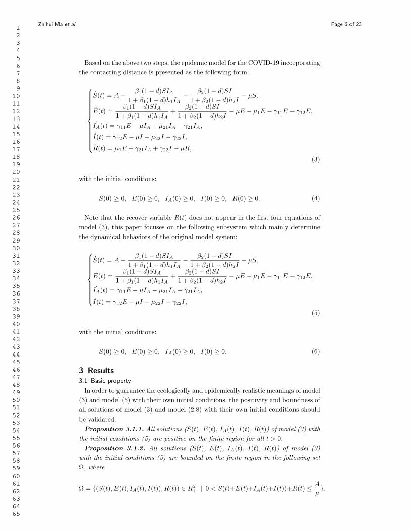
Based on the above two steps, the epidemic model for the COVID-19 incorporating
the contacting distance is presented as the following form:
S(t) = A−β1(1− d)SIA
1 + β1(1− d)h1IA−
β2(1− d)SI
1 + β2(1− d)h2I− µS,
E(t) =β1(1− d)SIA
1 + β1(1− d)h1IA+
β2(1− d)SI
1 + β2(1− d)h2I− µE − µ1E − γ11E − γ12E,
˙IA(t) = γ11E − µIA − µ21IA − γ21IA,
I(t) = γ12E − µI − µ22I − γ22I,
R(t) = µ1E + γ21IA + γ22I − µR,
(3)
with the initial conditions:
S(0) ≥ 0, E(0) ≥ 0, IA(0) ≥ 0, I(0) ≥ 0, R(0) ≥ 0. (4)
Note that the recover variable R(t) does not appear in the first four equations of
model (3), this paper focuses on the following subsystem which mainly determine
the dynamical behaviors of the original model system:
S(t) = A−β1(1− d)SIA
1 + β1(1− d)h1IA−
β2(1− d)SI
1 + β2(1− d)h2I− µS,
E(t) =β1(1− d)SIA
1 + β1(1− d)h1IA+
β2(1− d)SI
1 + β2(1− d)h2I− µE − µ1E − γ11E − γ12E,
˙IA(t) = γ11E − µIA − µ21IA − γ21IA,
I(t) = γ12E − µI − µ22I − γ22I,
(5)
with the initial conditions:
S(0) ≥ 0, E(0) ≥ 0, IA(0) ≥ 0, I(0) ≥ 0. (6)
3 Results3.1 Basic property
In order to guarantee the ecologically and epidemically realistic meanings of model
(3) and model (5) with their own initial conditions, the positivity and boundness of
all solutions of model (3) and model (2.8) with their own initial conditions should
be validated.
Proposition 3.1.1. All solutions (S(t), E(t), IA(t), I(t), R(t)) of model (3) with
the initial conditions (5) are positive on the finite region for all t > 0.
Proposition 3.1.2. All solutions (S(t), E(t), IA(t), I(t), R(t)) of model (3)
with the initial conditions (5) are bounded on the finite region in the following set
Ω, where
Ω = (S(t), E(t), IA(t), I(t)), R(t)) ∈ R5+ | 0 < S(t)+E(t)+IA(t)+I(t))+R(t) ≤
A
µ.
1
2
3
4
5
6
7
8
9
10
11
12
13
14
15
16
17
18
19
20
21
22
23
24
25
26
27
28
29
30
31
32
33
34
35
36
37
38
39
40
41
42
43
44
45
46
47
48
49
50
51
52
53
54
55
56
57
58
59
60
61
62
63
64
65
Zhihui Ma et al. Page 7 of 23
Based on the above theorems, the presented model (3) with the initial condi-
tions (5) is mathematically well-behaviored, and has its own epidemiological and
ecological meanings. Hence, the realistic aspects and properties of model (3) with
the initial conditions (5) are also guaranteed. Next, this paper focuses on the dy-
namical behaviors of model (3) with the initial conditions (5) and the theoretically
controlling methods for the epidemic diseases.
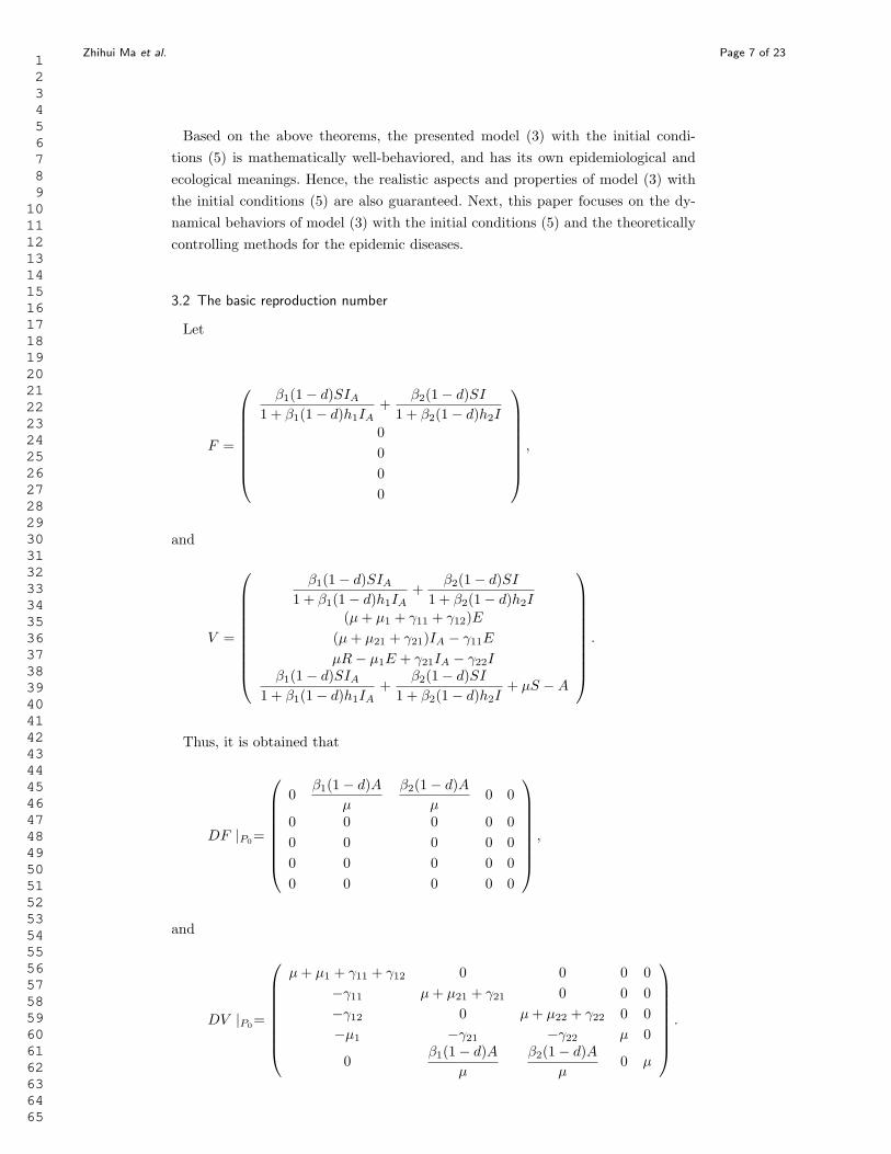
3.2 The basic reproduction number
Let
F =
β1(1− d)SIA1 + β1(1− d)h1IA
+β2(1− d)SI
1 + β2(1− d)h2I
0
0
0
0
,
and
V =
β1(1− d)SIA1 + β1(1− d)h1IA
+β2(1− d)SI
1 + β2(1− d)h2I
(µ+ µ1 + γ11 + γ12)E
(µ+ µ21 + γ21)IA − γ11E
µR− µ1E + γ21IA − γ22I
β1(1− d)SIA1 + β1(1− d)h1IA
+β2(1− d)SI
1 + β2(1− d)h2I+ µS −A
.
Thus, it is obtained that
DF |P0=
0β1(1− d)A
µ
β2(1− d)A
µ0 0
0 0 0 0 0
0 0 0 0 0
0 0 0 0 0
0 0 0 0 0
,
and
DV |P0=
µ+ µ1 + γ11 + γ12 0 0 0 0
−γ11 µ+ µ21 + γ21 0 0 0
−γ12 0 µ+ µ22 + γ22 0 0
−µ1 −γ21 −γ22 µ 0
0β1(1− d)A
µ
β2(1− d)A
µ0 µ
.
1
2
3
4
5
6
7
8
9
10
11
12
13
14
15
16
17
18
19
20
21
22
23
24
25
26
27
28
29
30
31
32
33
34
35
36
37
38
39
40
41
42
43
44
45
46
47
48
49
50
51
52
53
54
55
56
57
58
59
60
61
62
63
64
65
Zhihui Ma et al. Page 8 of 23
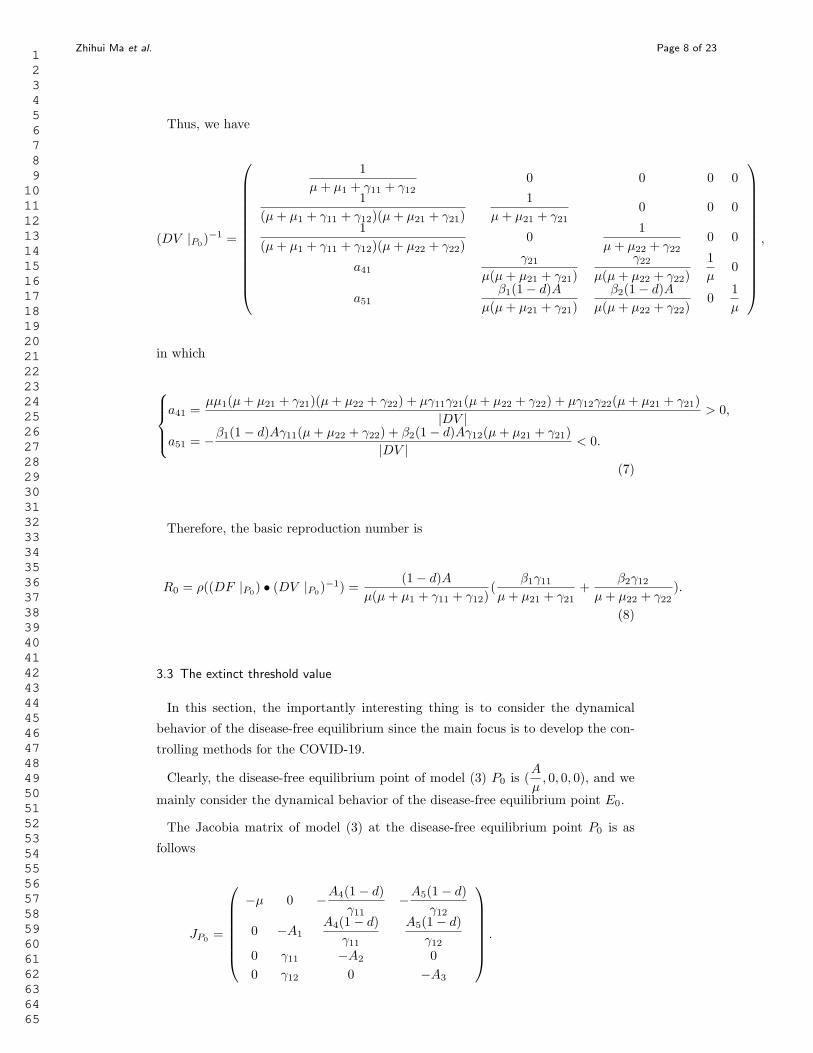
Thus, we have
(DV |P0)−1 =
1
µ+ µ1 + γ11 + γ120 0 0 0
1
(µ+ µ1 + γ11 + γ12)(µ+ µ21 + γ21)
1
µ+ µ21 + γ210 0 0
1
(µ+ µ1 + γ11 + γ12)(µ+ µ22 + γ22)0
1
µ+ µ22 + γ220 0
a41γ21
µ(µ+ µ21 + γ21)
γ22
µ(µ+ µ22 + γ22)
1
µ0
a51β1(1− d)A
µ(µ+ µ21 + γ21)
β2(1− d)A
µ(µ+ µ22 + γ22)0
1
µ
,
in which
a41 =µµ1(µ+ µ21 + γ21)(µ+ µ22 + γ22) + µγ11γ21(µ+ µ22 + γ22) + µγ12γ22(µ+ µ21 + γ21)
|DV |> 0,
a51 = −β1(1− d)Aγ11(µ+ µ22 + γ22) + β2(1− d)Aγ12(µ+ µ21 + γ21)
|DV |< 0.
(7)
Therefore, the basic reproduction number is
R0 = ρ((DF |P0) • (DV |P0
)−1) =(1− d)A
µ(µ+ µ1 + γ11 + γ12)(
β1γ11
µ+ µ21 + γ21+
β2γ12
µ+ µ22 + γ22).
(8)
3.3 The extinct threshold value
In this section, the importantly interesting thing is to consider the dynamical
behavior of the disease-free equilibrium since the main focus is to develop the con-
trolling methods for the COVID-19.
Clearly, the disease-free equilibrium point of model (3) P0 is (A
µ, 0, 0, 0), and we
mainly consider the dynamical behavior of the disease-free equilibrium point E0.
The Jacobia matrix of model (3) at the disease-free equilibrium point P0 is as
follows
JP0=
−µ 0 −A4(1− d)
γ11−A5(1− d)
γ12
0 −A1
A4(1− d)
γ11
A5(1− d)
γ120 γ11 −A2 0
0 γ12 0 −A3
.
1
2
3
4
5
6
7
8
9
10
11
12
13
14
15
16
17
18
19
20
21
22
23
24
25
26
27
28
29
30
31
32
33
34
35
36
37
38
39
40
41
42
43
44
45
46
47
48
49
50
51
52
53
54
55
56
57
58
59
60
61
62
63
64
65
Zhihui Ma et al. Page 9 of 23
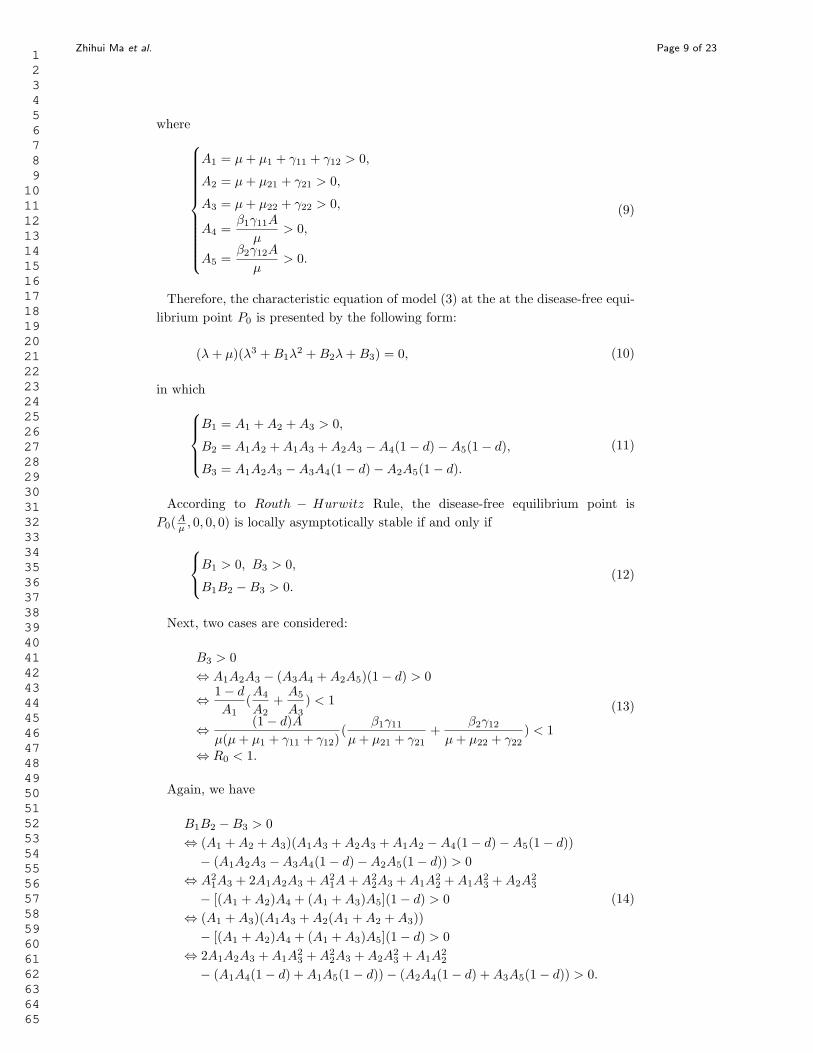
where
A1 = µ+ µ1 + γ11 + γ12 > 0,
A2 = µ+ µ21 + γ21 > 0,
A3 = µ+ µ22 + γ22 > 0,
A4 =β1γ11A
µ> 0,
A5 =β2γ12A
µ> 0.
(9)
Therefore, the characteristic equation of model (3) at the at the disease-free equi-
librium point P0 is presented by the following form:
(λ+ µ)(λ3 +B1λ2 +B2λ+B3) = 0, (10)
in which
B1 = A1 +A2 +A3 > 0,
B2 = A1A2 +A1A3 +A2A3 −A4(1− d)−A5(1− d),
B3 = A1A2A3 −A3A4(1− d)−A2A5(1− d).
(11)
According to Routh − Hurwitz Rule, the disease-free equilibrium point is
P0(Aµ, 0, 0, 0) is locally asymptotically stable if and only if
B1 > 0, B3 > 0,
B1B2 −B3 > 0.(12)
Next, two cases are considered:
B3 > 0
⇔ A1A2A3 − (A3A4 +A2A5)(1− d) > 0
⇔1− d
A1
(A4
A2
+A5
A3
) < 1
⇔(1− d)A
µ(µ+ µ1 + γ11 + γ12)(
β1γ11
µ+ µ21 + γ21+
β2γ12
µ+ µ22 + γ22) < 1
⇔ R0 < 1.
(13)
Again, we have
B1B2 −B3 > 0
⇔ (A1 +A2 +A3)(A1A3 +A2A3 +A1A2 −A4(1− d)−A5(1− d))
− (A1A2A3 −A3A4(1− d)−A2A5(1− d)) > 0
⇔ A21A3 + 2A1A2A3 +A2
1A+A22A3 +A1A
22 +A1A
23 +A2A
23
− [(A1 +A2)A4 + (A1 +A3)A5](1− d) > 0
⇔ (A1 +A3)(A1A3 +A2(A1 +A2 +A3))
− [(A1 +A2)A4 + (A1 +A3)A5](1− d) > 0
⇔ 2A1A2A3 +A1A23 +A2
2A3 +A2A23 +A1A
22
− (A1A4(1− d) +A1A5(1− d))− (A2A4(1− d) +A3A5(1− d)) > 0.
(14)
1
2
3
4
5
6
7
8
9
10
11
12
13
14
15
16
17
18
19
20
21
22
23
24
25
26
27
28
29
30
31
32
33
34
35
36
37
38
39
40
41
42
43
44
45
46
47
48
49
50
51
52
53
54
55
56
57
58
59
60
61
62
63
64
65

Zhihui Ma et al. Page 10 of 23
If R0 < 1, then we have
2A1A2A3 +A1A23 +A2
2A3 +A2A23 +A1A
22
−(A1A4(1− d) +A1A5(1− d))− (A2A4(1− d) +A3A5(1− d))
> (A1 +A2)(A1 +A+ 3) > 0.
(15)
Therefore, the disease-free equilibrium point is P0(Aµ, 0, 0, 0) is locally asymptoti-
cally stable if and only if
R0 < 1 ⇔ d > 1−µ(µ+ µ1 + γ11 + γ12)(µ+ µ22 + γ22)(µ+ µ21 + γ21)
β1γ11A(µ+ µ22 + γ22) + β2γ12A(µ+ µ21 + γ21)> 0.
(16)
Based on the above analysis, we obtain the following results.
Proposition 3.2.1. Suppose that β1γ11A(µ+µ22+γ22)+β2γ12A(µ+µ21+γ21) >
µ(µ+ µ1 + γ11 + γ12)(µ+ µ22 + γ22)(µ+ µ21 + γ21), we have
(1). If R0 > 1 or d < 1 −µ(µ+ µ1 + γ11 + γ12)(µ+ µ22 + γ22)(µ+ µ21 + γ21)
β1γ11A(µ+ µ22 + γ22) + β2γ12A(µ+ µ21 + γ21),
then the disease-free equilibrium point P0 is unstable,
(2). If R0 < 1 or d > 1 −µ(µ+ µ1 + γ11 + γ12)(µ+ µ22 + γ22)(µ+ µ21 + γ21)
β1γ11A(µ+ µ22 + γ22) + β2γ12A(µ+ µ21 + γ21),
then the disease-free equilibrium point P0 is locally asymptotically stable.
Proposition 3.2.1 reveals that the COVID-19 can be controlled while the contact-
ing distance between the healthy individuals and the symptomatic infected individu-
als is larger than the threshold value d∗ = 1−µ(µ+ µ1 + γ11 + γ12)(µ+ µ22 + γ22)(µ+ µ21 + γ21)
β1γ11A(µ+ µ22 + γ22) + β2γ12A(µ+ µ21 + γ21).
This threshold value decreases with the decrease in the immigration rate of suscep-
tible population.
3.4 Model (3) without the asymptomatic infected population
If the asymptomatic infected population is omitted since it is difficult to be found
and the infection probability of the asymptomatic individuals is very small, then
the model (3) will become the following forms
S(t) = A−β2(1− d)SI
1 + β2(1− d)h2I− µS,
E(t) =β2(1− d)SI
1 + β2(1− d)h2I− µE − µ1E − γ12E,
I(t) = γ12E − µI − µ22I − γ22I,
(17)
with the initial conditions:
S(0) ≥ 0, E(0) ≥ 0, I(0) ≥ 0. (18)
According to Proposition 3.1.1 and Proposition 3.1.2, all solutions of model (17)
with the initial conditions (18) are positive and bounded.
1
2
3
4
5
6
7
8
9
10
11
12
13
14
15
16
17
18
19
20
21
22
23
24
25
26
27
28
29
30
31
32
33
34
35
36
37
38
39
40
41
42
43
44
45
46
47
48
49
50
51
52
53
54
55
56
57
58
59
60
61
62
63
64
65
Zhihui Ma et al. Page 11 of 23
According to the computation of the basic reproduction number of model (3) R0,
the basic reproduction number of model(17) is
R0 =β2γ12A(1− d)
µ(µ+ µ1 + γ12)(µ+ µ22 + γ22), (19)
By simple computation, the disease-free equilibrium point of model (17) is
P0(A
µ, 0, 0) and the corresponding endemic equilibrium point is P (S, E, I), where
S =β2γ12(1− d) + µ(µ+ µ1 + γ12)(µ+ µ22 + γ22)
β2γ12(1− d)(µh2 + 1),
E =β2γ12(1− d)− µ(µ+ µ1 + γ12)(µ+ µ22 + γ22)
β2γ12(1− d)(µh2 + 1)(µ+ µ1 + γ12),
I =β2γ12(1− d)− µ(µ+ µ1 + γ12)(µ+ µ22 + γ22)
β2γ12(1− d)(µh2 + 1)(µ+ µ1 + γ12)(µ+ µ22 + γ22).
(20)
Clearly, the endemic equilibrium point P is positive if and only if R0 > 1.
Next, the stability properties of the disease-free equilibrium point P0 and the
endemic equilibrium point P are considered.
Firstly, the Jacobia matrix of model (17) at the disease-free equilibrium point P0
is as follows
JP0=
−µ 0 −β2A(1− d)
µ
0 −A1
β2A(1− d)
µ
0 γ12 −A3
.
The corresponding characteristic equation of model (17) at the disease-free equi-
librium point P0 is
(λ+ µ)(λ2 + (A1 +A3)λ+A1A3 −A5(1− d)), (21)
Therefore, according to Routh−Hurwitz Rule, the disease-free equilibrium point
is P0 is locally asymptotically stable if and only if
A1A3 −A5(1− d) > 0
⇔A5(1− d)
A1A3
< 1
⇔ R0 < 1
⇔ d > 1−µ(µ+ µ1 + γ12)(µ+ µ22 + γ22)
β2Aγ12> 0.
(22)
Secondly, the Jacobia matrix of model (17) at the endemic equilibrium point P
is as follows
JP =
−µ−β2A(1− d)I
1 + β2(1− d)h2I0
β2(1− d)((µ+ µ1 + γ12)(µ+ µ22 + γ22)− γ12A)
µγ12(1 + β2(1− d)h2I)2
β2A(1− d)I
1 + β2(1− d)h2I−(µ+ µ1 + γ12)
β2(1− d)(γ12A− (µ+ µ1 + γ12)(µ+ µ22 + γ22))
µγ12(1 + β2(1− d)h2I)2
0 γ12 −(µ+ µ22 + γ22)
.
1
2
3
4
5
6
7
8
9
10
11
12
13
14
15
16
17
18
19
20
21
22
23
24
25
26
27
28
29
30
31
32
33
34
35
36
37
38
39
40
41
42
43
44
45
46
47
48
49
50
51
52
53
54
55
56
57
58
59
60
61
62
63
64
65
Zhihui Ma et al. Page 12 of 23
The corresponding characteristic equation of model (17) at the endemic equilib-
rium point P is
λ3 + B1λ2 + B2λ+ B3, (23)
where
B1 =β2γ12A(1− d)(µh2 + 1)
β2γ12h2(1− d) +A1A2
+A1 +A2,
B2 =A1A2h2(β2γ12A(1− d)− µA1A2) + β2γ12A(1− d)(µh2 + 1)(A1 +A2)
β2γ12h2(1− d) +A1A2
,
B3 =A1A2(µh2 + 1)(β2γ12A(1− d)− µA1A2)
β2γ12h2(1− d) +A1A2
.
(24)
According to Routh−Hurwitz Rule, the endemic equilibrium point P is locally
asymptotically stable if and only if
B1 > 0, B3 > 0,
B1B2 − B3 > 0.(25)
Clearly, the term B1 > 0 and B3 > 0 hold if R0 > 1 or d < 1 −µ(µ+ µ1 + γ12)(µ+ µ22 + γ22)
β2Aγ12.
Again, we have
B1B2 − B3 > 0
⇔β2γ12A(1− d)(µh2 + 1)(A1 +A2)
2
β2γ12Ah2(1− d) +A1A2
−A1A2h2(β2γ12A(1− d)− µA1A2)
β2γ12Ah2(1− d) +A1A2
> 0
⇔(µh2 + 1)(γ12A(1− d)(A2
1 +A22 +A1A2) + µA2
1A22)
β2γ12Ah2(1− d) +A1A2
> 0.
(26)
Based on the above analysis, we obtain the following results.
Proposition 3.3.1. Suppose that β2Aγ12 > µ(µ + µ1 + γ12)(µ + µ22 + γ22), we
have
(1). If R0 > 1 or d < 1−µ(µ+ µ1 + γ12)(µ+ µ22 + γ22)
β2Aγ12, then the endemic equi-
librium point P is locally asymptotically stable,
(2). If R0 < 1 or d > 1 −µ(µ+ µ1 + γ12)(µ+ µ22 + γ22)
β2Aγ12, then the disease-free
equilibrium point P0 is locally asymptotically stable.
Proposition 3.3.1 reveals that the COVID-19, which incorporates the relatively
high infection rate, can be controlled while the contacting distance between the
healthy individuals and the symptomatic infected individuals is larger than the
threshold value d∗ = 1−µ(µ+ µ1 + γ12)(µ+ µ22 + γ22)
β2Aγ12. This threshold value de-
creases with the decrease in the immigration rate of susceptible population. That
is to say, the contacting distance could be shortened in the locations with the low
1
2
3
4
5
6
7
8
9
10
11
12
13
14
15
16
17
18
19
20
21
22
23
24
25
26
27
28
29
30
31
32
33
34
35
36
37
38
39
40
41
42
43
44
45
46
47
48
49
50
51
52
53
54
55
56
57
58
59
60
61
62
63
64
65
Zhihui Ma et al. Page 13 of 23
population density. The equivalent results of Proposition 3.2.1, which take the im-
migration rate of susceptible population as the controlling parameter, can also be
proposed as follows.
Proposition 3.3.2. We have the following conclusions
(1). If 0 < A <µ(µ+ µ1 + γ12)(µ+ µ22 + γ22)
β2γ12(1− d), then the disease-free equilibrium
point P0 is locally asymptotically stable,
(2). Ifµ(µ+ µ1 + γ12)(µ+ µ22 + γ22)
β2γ12(1− d)< A < 1, then the endemic equilibrium
point P is locally asymptotically stable.
Proposition 3.3.2 reveals that the COVID-19 can be controlled while the im-
migration rate of susceptible population is smaller than the threshold value A∗ =µ(µ+ µ1 + γ12)(µ+ µ22 + γ22)
β2(1− d), and this threshold value increases with the increase
in the contacting distance between the healthy individuals and the symptomatic in-
fected individuals. That is to say, only if the contacting distance is large enough,
the relatively large immigration of local peoples can not induce the second outbreak
of the COVID-19.
3.5 Sensitivity analysis
In this section, the numerical test for model (17) is conducted based on the re-
ported cases induced by the COVID-19 in Wuhan in Hubei province and the esti-
mated parameters of the published works (Li et al., 2020; Tang et al., 2020). All
parameter values are given in the following Table 1.
Table 1. The estimated values of parameters in model (17)
Parameter Definitions Mean value Source
A The infux of the susceptible subpopulation Variableβ2 The intrinsically infectious rate 0.8 Li and Tang et al.h2 The average outdoor-time of each asymptomatic infected individual 0.5 Li and Tang et al.µ The natural death rates of all subpopulations 0.00711 Li et al., Tang et al.µ1 The recovery rate of the incubation subpopulation 0.13978 Li and Tang et al.µ22 The death rate induced bythe coronavirus disease 2019 (COVID-19) 0.04017 Li and Tang et al.γ12 The transition rate from the incubation subpopulation
to the symptomatic infected subpopulation 0.07143—0.19231 Li and Tang et al.γ22 The recovery rate of the symptomatic infected subpopulation 0.33029 Tang et al.d The contacting distance between the susceptible individuals
and the asymptomatic infected individuals Variable 0 ≤ d ≤ 1
In order to identify the key factors affecting the change of infection variables, we
used Latin Hypercube Sampling (LHS) for parameter sampling and Paranoid Rank
Correlation Coefficient (PRCC) method for sensitivity analysis of the parameters
in the model (17). When performing parameter sampling, we choose uniform dis-
tribution as the prior distribution, sampling times N = 500, the reference values of
the parameters in the model are given in Table 1, and the value range is 20% up
and down the reference value. The parameters with p value greater than 0.01 are
considered to have no effect on the model.
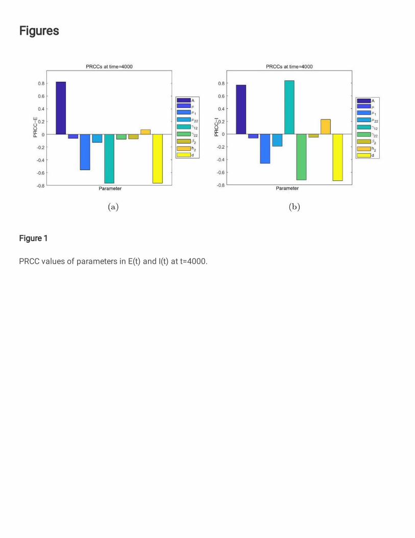
From Figure 1(a) and Table 2, it can be seen that parameter A and E(t) are
positively correlated, that is, as parameter A increases, the population of E(t)
subgroups will increase. µ1, γ12, d are negatively correlated with E(t), that is,
increasing µ1, γ12, d will cause E(t) to decrease. It can be seen from the Figure
1
2
3
4
5
6
7
8
9
10
11
12
13
14
15
16
17
18
19
20
21
22
23
24
25
26
27
28
29
30
31
32
33
34
35
36
37
38
39
40
41
42
43
44
45
46
47
48
49
50
51
52
53
54
55
56
57
58
59
60
61
62
63
64
65

Zhihui Ma et al. Page 14 of 23
Table 2. PRCC value and P value of each parameter in E(t)
Parameter PRCC values P value Parameter PRCC values P value
A 0.8300 0.0000 γ22 −0.0743 0.3216µ −0.0453 0.2541 β2 −0.0685 0.9217µ1 −0.5824 0.0000 h2 0.6829 0.1787µ22 −0.1399 0.0175 d 0.7539 0.0000γ12 −0.7678 0.0000
Table 3. PRCC value and P value of each parameter in I(t)
Parameter PRCC values P value Parameter PRCC values P value
A 0.7808 0.0000 γ22 −0.7437 0.0000µ −0.1049 0.9927 β2 −0.0483 0.7827µ1 −0.4824 0.0000 h2 0.2149 0.6722µ22 −0.1951 0.0109 d 0.7538 0.0000γ12 0.8374 0.0000
2 that the monotonicity of A, µ1, γ12, d is the most significant, that is, E(t) is
mainly affected by these parameters. Figure 1(b) and Table 3 shows that A and
γ12 are positively correlated with I(t), that is, as A and γ12 increase, I(t) will
increase. µ1, γ22, d and I(t) are negatively correlated, that is, as µ1, γ22, d increase,
the population of I(t) will decrease. It can be seen from the Figure 3 that the
monotonicity of A, µ1, γ12,γ22, d is the most significant, in other words, I(t) is
mainly affected by these parameters.
(a) (b)
Figure 1: PRCC values of parameters in E(t) and I(t) at t=4000.
It can be seen from Figure 4 that the PRCC value of each parameter changes
significantly in the early stage of the outbreak, especially before t = 500. It can be
seen from (b) that the parameters A, µ1, γ12, γ22 and d have undergone significant
changes relative to I(t). The PRCC values of A and d show a trend of first increasing,
then decreasing and then increasing over time. This is due to the rapid increase in
the number of patients after the outbreak, and the susceptible subpopulation S(t)
is more likely to be infected under the same d as the initial outbreak. At this
time, social distance d will have a greater impact on the number of patients. With
the improvement of people’s awareness of the prevention of epidemics and medical
conditions, people’s behavior of reducing overtime and using masks will lead to less
and less impact of d on I(t). Due to the phased results of the epidemic prevention
1
2
3
4
5
6
7
8
9
10
11
12
13
14
15
16
17
18
19
20
21
22
23
24
25
26
27
28
29
30
31
32
33
34
35
36
37
38
39
40
41
42
43
44
45
46
47
48
49
50
51
52
53
54
55
56
57
58
59
60
61
62
63
64
65
Zhihui Ma et al. Page 15 of 23
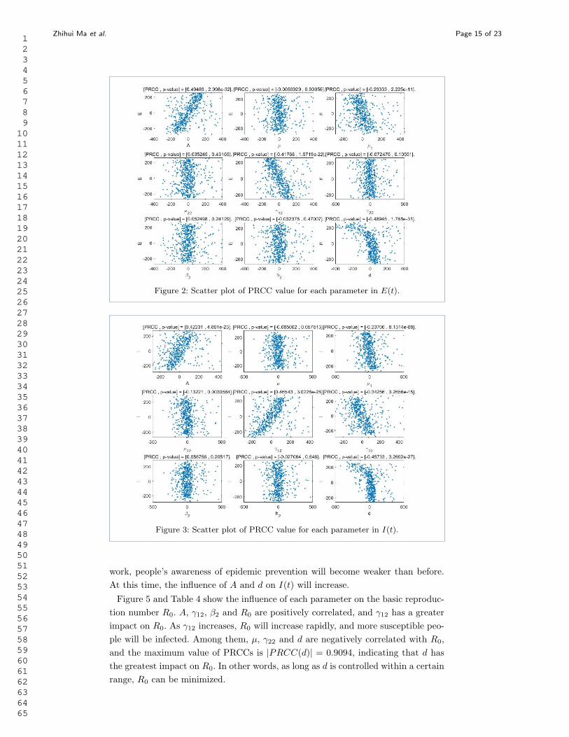
Figure 2: Scatter plot of PRCC value for each parameter in E(t).
Figure 3: Scatter plot of PRCC value for each parameter in I(t).
work, people’s awareness of epidemic prevention will become weaker than before.
At this time, the influence of A and d on I(t) will increase.
Figure 5 and Table 4 show the influence of each parameter on the basic reproduc-
tion number R0. A, γ12, β2 and R0 are positively correlated, and γ12 has a greater
impact on R0. As γ12 increases, R0 will increase rapidly, and more susceptible peo-
ple will be infected. Among them, µ, γ22 and d are negatively correlated with R0,
and the maximum value of PRCCs is |PRCC(d)| = 0.9094, indicating that d has
the greatest impact on R0. In other words, as long as d is controlled within a certain
range, R0 can be minimized.
1
2
3
4
5
6
7
8
9
10
11
12
13
14
15
16
17
18
19
20
21
22
23
24
25
26
27
28
29
30
31
32
33
34
35
36
37
38
39
40
41
42
43
44
45
46
47
48
49
50
51
52
53
54
55
56
57
58
59
60
61
62
63
64
65

Zhihui Ma et al. Page 16 of 23
(a) (b)
Figure 4: PRCC value of each parameter over time.
Table 4. PRCC value and P value of each parameter in R0
Parameter PRCC values P value Parameter PRCC values P value
A 0.1608 0.0000 γ22 −0.1103 0.0000µ −0.1737 0.0000 β2 0.1587 0.0000µ1 −0.0517 0.0207 h2 0.004 0.8582µ22 −0.0077 0.7307 d −0.9094 0.0000γ12 0.2112 0.0000
Figure 5: PRCC values of each parameter in R0.
3.6 Numerical test
According to Proposition 3.3.1 and Proposition 3.3.2, the threshold values of
the contacting distance d∗ and the immigration rate A∗ are 0.8767 and 0.1849,
respectively. That is to say, the COVID-19 will be completely controlled when the
contacting distance is larger than the threshold value 0.8767, or the immigration
rate smaller than the threshold value 0.1849. Here, the immigration rate measures
the density of population who immigrates to the streets from their own home in
Wuhan city.
1
2
3
4
5
6
7
8
9
10
11
12
13
14
15
16
17
18
19
20
21
22
23
24
25
26
27
28
29
30
31
32
33
34
35
36
37
38
39
40
41
42
43
44
45
46
47
48
49
50
51
52
53
54
55
56
57
58
59
60
61
62
63
64
65

Zhihui Ma et al. Page 17 of 23
Figure 6: The disease-free equilibrium point P0 is globally asymptotically stable withd = 0.89 which is larger than the threshold value 0.8767.
(a) (b)
Figure 7: The time-series diagrams for E and I with the different contacting
distances while it is larger than the threshold value 0.8767.
Figure 6—Figure 8 show that the COVID-19 will be completely controlled when
the contacting distance is larger than the threshold value 0.8767. Figure 6 selects
the contacting distance between the susceptible individuals and the symptomatic in-
fected individuals as 0.89 which is larger than the threshold value 0.8767, and hence
that the COVID-19 will be vanished. Noting that the parameter of the contacting
distance is normalized in the modeling processes, hence, for the COVID-19, it will
be completely controlled only if the susceptible individuals and the symptomatic
infected individuals keep their contacting distance to be larger than 0.8767 × D,
where D is the spread distance of the coronavirus of the COVID-19 when people
are breathing and/or sneezing. Generally, individuals are require to keep away at
least one meter. Furthermore, Figure 7 reveals that the extinct lag of the COVID-19
closely relates to the contacting distance when the peoples’ immigrating number is
30 percent of the total population in Wuhan city after January 23th, 2020, and the
1
2
3
4
5
6
7
8
9
10
11
12
13
14
15
16
17
18
19
20
21
22
23
24
25
26
27
28
29
30
31
32
33
34
35
36
37
38
39
40
41
42
43
44
45
46
47
48
49
50
51
52
53
54
55
56
57
58
59
60
61
62
63
64
65
Zhihui Ma et al. Page 18 of 23
(a) (b)
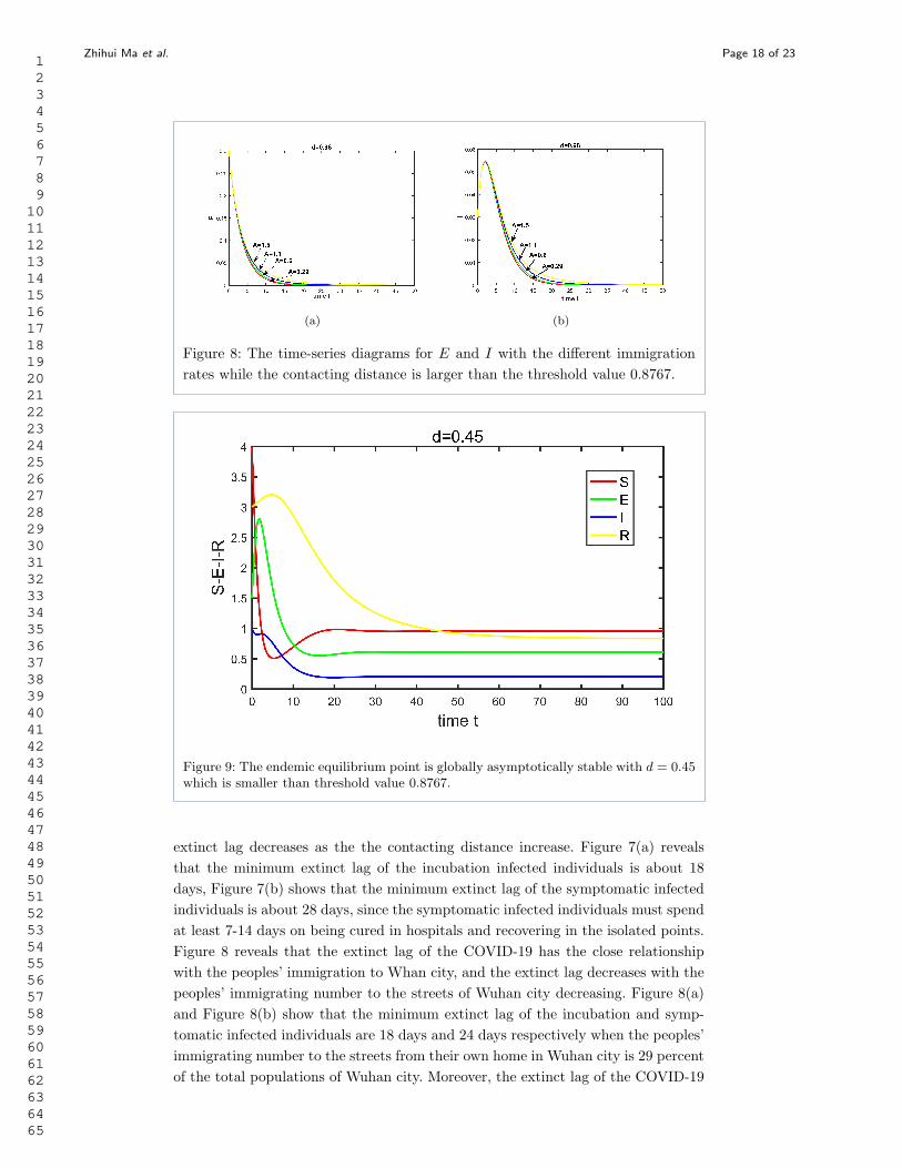
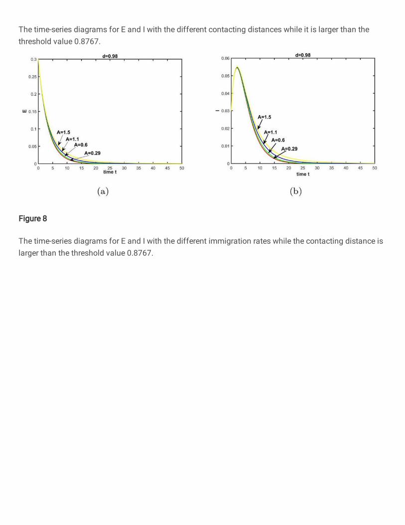
Figure 8: The time-series diagrams for E and I with the different immigration
rates while the contacting distance is larger than the threshold value 0.8767.
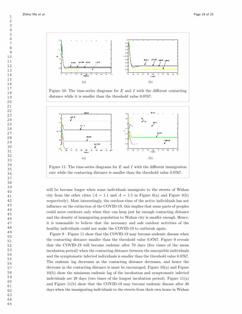
Figure 9: The endemic equilibrium point is globally asymptotically stable with d = 0.45which is smaller than threshold value 0.8767.
extinct lag decreases as the the contacting distance increase. Figure 7(a) reveals
that the minimum extinct lag of the incubation infected individuals is about 18
days, Figure 7(b) shows that the minimum extinct lag of the symptomatic infected
individuals is about 28 days, since the symptomatic infected individuals must spend
at least 7-14 days on being cured in hospitals and recovering in the isolated points.
Figure 8 reveals that the extinct lag of the COVID-19 has the close relationship
with the peoples’ immigration to Whan city, and the extinct lag decreases with the
peoples’ immigrating number to the streets of Wuhan city decreasing. Figure 8(a)
and Figure 8(b) show that the minimum extinct lag of the incubation and symp-
tomatic infected individuals are 18 days and 24 days respectively when the peoples’
immigrating number to the streets from their own home in Wuhan city is 29 percent
of the total populations of Wuhan city. Moreover, the extinct lag of the COVID-19
1
2
3
4
5
6
7
8
9
10
11
12
13
14
15
16
17
18
19
20
21
22
23
24
25
26
27
28
29
30
31
32
33
34
35
36
37
38
39
40
41
42
43
44
45
46
47
48
49
50
51
52
53
54
55
56
57
58
59
60
61
62
63
64
65
Zhihui Ma et al. Page 19 of 23
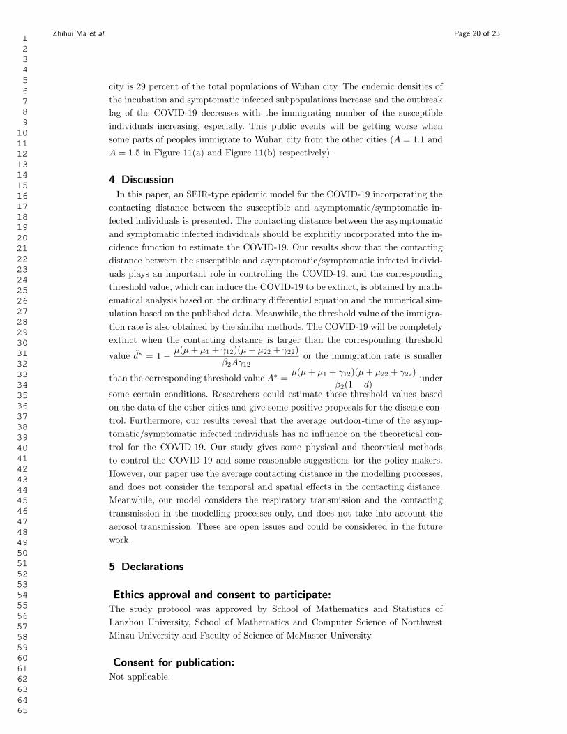
(a) (b)
Figure 10: The time-series diagrams for E and I with the different contacting
distance while it is smaller than the threshold value 0.8767.
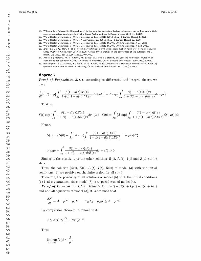
(a) (b)
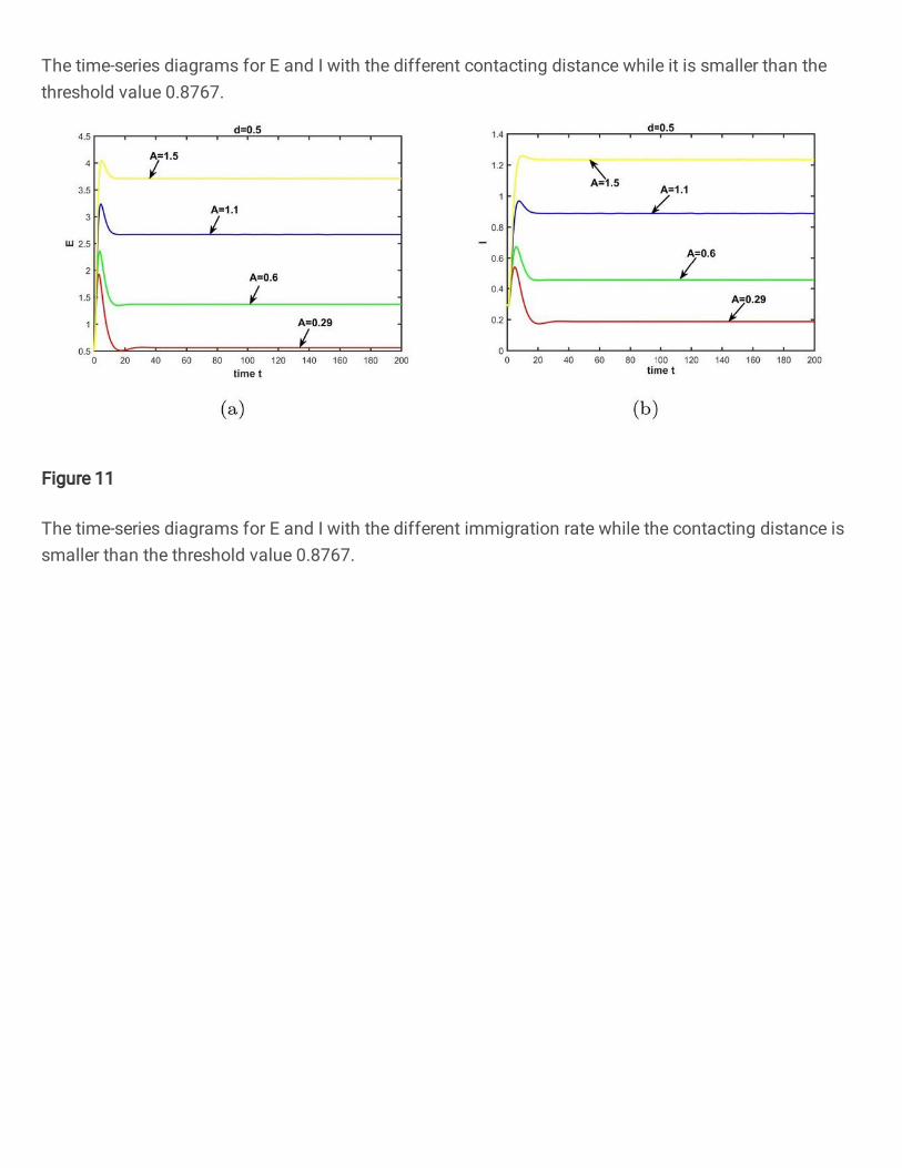
Figure 11: The time-series diagrams for E and I with the different immigration
rate while the contacting distance is smaller than the threshold value 0.8767.
will be become longer when some individuals immigrate to the streets of Wuhan
city from the other cities (A = 1.1 and A = 1.5 in Figure 8(a) and Figure 8(b)
respectively). Most interestingly, the outdoor-time of the active individuals has not
influence on the extinction of the COVID-19, this implies that some parts of peoples
could move outdoors only when they can keep just far enough contacting distance
and the density of immigrating population to Wuhan city is smaller enough. Hence,
it is reasonable to believe that the necessary and safe outdoor activities of the
healthy individuals could not make the COVID-19 to outbreak again.
Figure 9—Figure 11 show that the COVID-19 may become endemic disease when
the contacting distance smaller than the threshold value 0.8767. Figure 9 reveals
that the COVID-19 will become endemic after 70 days (five times of the mean
incubation period) when the contacting distance between the susceptible individuals
and the symptomatic infected individuals is smaller than the threshold value 0.8767.
The endemic lag decreases as the contacting distance decreases, and hence the
decrease in the contacting distance is must be encouraged. Figure 10(a) and Figure
10(b) show the minimum endemic lag of the incubation and symptomatic infected
individuals are 28 days (two times of the longest incubation period). Figure 11(a)
and Figure 11(b) show that the COVID-19 may become endemic disease after 38
days when the immigrating individuals to the streets from their own home in Wuhan
1
2
3
4
5
6
7
8
9
10
11
12
13
14
15
16
17
18
19
20
21
22
23
24
25
26
27
28
29
30
31
32
33
34
35
36
37
38
39
40
41
42
43
44
45
46
47
48
49
50
51
52
53
54
55
56
57
58
59
60
61
62
63
64
65
Zhihui Ma et al. Page 20 of 23
city is 29 percent of the total populations of Wuhan city. The endemic densities of
the incubation and symptomatic infected subpopulations increase and the outbreak
lag of the COVID-19 decreases with the immigrating number of the susceptible
individuals increasing, especially. This public events will be getting worse when
some parts of peoples immigrate to Wuhan city from the other cities (A = 1.1 and
A = 1.5 in Figure 11(a) and Figure 11(b) respectively).
4 Discussion
In this paper, an SEIR-type epidemic model for the COVID-19 incorporating the
contacting distance between the susceptible and asymptomatic/symptomatic in-
fected individuals is presented. The contacting distance between the asymptomatic
and symptomatic infected individuals should be explicitly incorporated into the in-
cidence function to estimate the COVID-19. Our results show that the contacting
distance between the susceptible and asymptomatic/symptomatic infected individ-
uals plays an important role in controlling the COVID-19, and the corresponding
threshold value, which can induce the COVID-19 to be extinct, is obtained by math-
ematical analysis based on the ordinary differential equation and the numerical sim-
ulation based on the published data. Meanwhile, the threshold value of the immigra-
tion rate is also obtained by the similar methods. The COVID-19 will be completely
extinct when the contacting distance is larger than the corresponding threshold
value d∗ = 1 −µ(µ+ µ1 + γ12)(µ+ µ22 + γ22)
β2Aγ12or the immigration rate is smaller
than the corresponding threshold value A∗ =µ(µ+ µ1 + γ12)(µ+ µ22 + γ22)
β2(1− d)under
some certain conditions. Researchers could estimate these threshold values based
on the data of the other cities and give some positive proposals for the disease con-
trol. Furthermore, our results reveal that the average outdoor-time of the asymp-
tomatic/symptomatic infected individuals has no influence on the theoretical con-
trol for the COVID-19. Our study gives some physical and theoretical methods
to control the COVID-19 and some reasonable suggestions for the policy-makers.
However, our paper use the average contacting distance in the modelling processes,
and does not consider the temporal and spatial effects in the contacting distance.
Meanwhile, our model considers the respiratory transmission and the contacting
transmission in the modelling processes only, and does not take into account the
aerosol transmission. These are open issues and could be considered in the future
work.
5 Declarations
Ethics approval and consent to participate:The study protocol was approved by School of Mathematics and Statistics of
Lanzhou University, School of Mathematics and Computer Science of Northwest
Minzu University and Faculty of Science of McMaster University.
Consent for publication:Not applicable.
1
2
3
4
5
6
7
8
9
10
11
12
13
14
15
16
17
18
19
20
21
22
23
24
25
26
27
28
29
30
31
32
33
34
35
36
37
38
39
40
41
42
43
44
45
46
47
48
49
50
51
52
53
54
55
56
57
58
59
60
61
62
63
64
65

Zhihui Ma et al. Page 21 of 23
Availability of data and material:The data set used and/or analyzed during the current study is available from the
published works.
Conflicts of Interest:The authors declare no conflict of interest.
FundingThis work was supported by Natural Science Foundation of Gansu Province (No.
20JR5RA238) and Fundamental Research Funds for the Central Universities of
Northwest Minzu University (No. 31920190089).
CRediT authorship contribution statementZ. Ma, Conceptualization, Methodology, Writing-review and editing; S. Wang and
H. Liu, Writing-review and editing; X. Li, X. Li, X. Han and H. Wang Software,
Writing-editing.
Acknowledgements:Not applicable.
Author details1School of Mathematics and Statistics, Lanzhou University, Lanzhou,Gansu 730000, People’s Republic of China.2School of Mathematics and Computer Science, Northwest Minzu University, Lanzhou,Gansu 730000, People’s
Republic of China. 3Faculty of Science, McMaster University, Hamilton,Ontario,L8S4L8, Canada.
References
1. Bogardus, E. Measuring social distance. Journal of Applied Sociology, 1925, 9, 299-308.
2. Chen, Y.; Liu, Q.; Guo, D. Coronaviruses: Genome structure, replication, and pathogenesis. J. Med. Virol.
2020;92:418-423.
3. Cheng, V. C. C.; Wong, S. C.; To, K. K. W.; Ho, P. L.; Yuen, K. Y. Preparedness and proactive infection control
measures against the emerging Wuhan coronavirus pneumonia in China. J. Hosp. Infect. 2020, 104(3), 254-255
4. De Wit, E.; van Doremalen, N.; Falzarano, D.; Munster, V.J. SARS and MERS: Recent insights into emerging
coronaviruses. Nat. Rev. Microbiol. 2016, 14, 523-534.
5. Hui, D. S. C.; Zumla, A. Severe acute respiratory syndrome: Historical, epidemiologic, and clinical features.
Infect. Dis. Clin. North Am. 2019, 33, 869-889.
6. Ma, Z., Wang, S., Li, H., A generalized infectious model induced by the contacting distance, Nonlinear
Anal-Real. 54 (2020) 103113.
7. Hodgetts, D.; Stolte, O.; Radley, A.; Leggatt-Cook, C.; Groot, S.; Chamberlain, K. “Near and far”: Social
distancing in domiciled characterizations of homeless people. Urban Studies, 2011, 48(8), 1739-1754.
8. Kahn, J.S.; McIntosh, K. History and recent advances in coronavirus discovery. Pediatr. Infect. Dis. J. 2005, 24,
S223-227.
9. Killerby, M. E.; Biggs, H. M.; Midgley, C. M.; Gerber, S.I.; Watson, J.T. Middle East respiratory syndrome
coronavirus transmission. Emerg. Infect. Dis. 2020, 26, 191-198.
10. Kwok, K. O.; Tang, A.; Wei, V. W. I.; Park, W. H.; Yeoh, E. K.; Riley, S. Epidemic models of contact tracing:
Systematic review of transmission studies of severe acute respiratory syndrome and Middle East respiratory
syndrome. Comput. Struct. Biotechnol. J. 2019, 17, 186-194.
11. Li, Q.; Guan, X.; Peng, Wu P.; et al. Early Transmission Dynamics in Wuhan, China, of Novel
Coronavirus-nfected Pneumonia. New. Engl. J. Med. 2020, 382(13), 1199-1207.
12. Ma, Z.; Wang, S.; Li X. A generalized infectious model induced by the contacting distance (CTD). Nonlinear
Anal. RWA. 2020, 54,103113.
13. M. Simeone, B. H. Ian, J. R. Christian, et al. A methodology for performing global uncertainty and sensitivity
analysis in systems biology,J.Theor.Biol.,254(2008), 178-196.
14. National Health Commission of the People’s Republic of China (NHCPRC). Available online:
http://www.nhc.gov.cn/xcs/yqtb/202002/ac1e98495cb04d36b0d0a4e1e7fab545.shtml (Report on February
21th 2020).
15. National Health Commission of the People’s Republic of China (NHCPRC). Available online:
http://www.nhc.gov.cn/xcs/yqtb/202001/c5da49c4c5bf4bcfb320ec2036480627.shtml (Report on January
24th 2020).
16. Rothe, C.; Schunk, M.; Sothmann, P.; et al. Transmission of 2019-nCoV infection from an asymptomatic
contact in Germany. N. Engl. J. Med. 2020, 10, 1-3.
17. Tang, B.; Wang, X.; Li, Q.; Bragazzi, N. L.; Tang, S.; Xiao, Y.; Wu, J. Estimation of the Transmission Risk of
the 2019-nCoV and Its Implication for Public Health Interventions. J. Clin. Med. 2020, 9(2), 462-474.
1
2
3
4
5
6
7
8
9
10
11
12
13
14
15
16
17
18
19
20
21
22
23
24
25
26
27
28
29
30
31
32
33
34
35
36
37
38
39
40
41
42
43
44
45
46
47
48
49
50
51
52
53
54
55
56
57
58
59
60
61
62
63
64
65
Zhihui Ma et al. Page 22 of 23
18. Willman, M.; Kobasa, D.; Kindrachuk, J. A Comparative analysis of factors influencing two outbreaks of middle
eastern respiratory syndrome (MERS) in Saudi Arabia and South Korea. Viruses 2019, 11, E1119.
19. World Health Organization (WHO). Coronavirus disease 2019 (2019-nCoV) Situation Report-4. 2020.
20. World Health Organization (WHO), Novel Coronavirus (2019-nCoV) Situation Report-22. 2020.
21. World Health Organization (WHO). Coronavirus disease 2019 (COVID-19) Situation Report-31. 2020.
22. World Health Organization (WHO). Coronavirus disease 2019 (COVID-19) Situation Report-112. 2020.
23. Zhao, S.; Lin, Q.; Ran, J.; et al. Preliminary estimation of the basic reproduction number of novel coronavirus
(2019-nCoV) in China, from 2019 to 2020: A data-driven analysis in the early phase of the outbreak. Int. J.
Infect. Dis. 2020, doi:10.1016/j.ijid.2020.01.050.
24. Annas, S.; Pratama, M. S.; Rifandi, M.; Sanusi, W.; Side, S.; Stability analysis and numerical simulation of
SEIR model for pandemic COVID-19 spread in Indonesia, Chaos, Solitons and Fractals. 139 (2020) 110072.
25. Boukanjimea, B.; Caraballo, T.; Fatini, M. E.; Khalif, M. E.; Dynamics of a stochastic coronavirus (COVID-19)
epidemic model with Markovian switching, Chaos, Solitons and Fractals. 141 (2020) 110361.
AppendixProof of Proposition 3.1.1. According to differential and integral theory, we
have
d
dt[S(t) exp
∫ t
0
β(1− d(τ))E(τ)
1 + β(1− d(τ))hE(τ)dτ+µt] = A exp
∫ t
0
β(1− d(τ))E(τ)
1 + β(1− d(τ))hE(τ)dτ+µt.
That is,
S(t) exp
∫ t
0
β(1− d(τ))E(τ)
1 + β(1− d(τ))hE(τ)dτ+µt−S(0) =
∫ t
0
[A exp
∫ t
0
β(1− d(τ))E(τ)
1 + β(1− d(τ))hE(τ)dτ+µt]dt.
Hence,
S(t) = S(0) +
∫ t
0
[A exp
∫ t
0
β(1− d(τ))E(τ)
1 + β(1− d(τ))hE(τ)dτ + µt]dt
× exp−
∫ t
0
β(1− d(τ))E(τ)
1 + β(1− d(τ))hE(τ)dτ + µt > 0.
Similarly, the positivity of the other solutions E(t), IA(t), I(t) and R(t) can be
shown.
Thus, the solution (S(t), E(t), IA(t), I(t), R(t)) of model (3) with the initial
conditions (4) are positive on the finite region for all t > 0.
Therefore, the positivity of all solutions of model (5) with the initial conditions
(6) is also guaranteed since model (3) is a special case of model (4).
Proof of Proposition 3.1.2. Define N(t) = S(t) + E(t) + IA(t) + I(t) + R(t)
and add all equations of model (3), it is obtained that
dN
dt= A− µN − µ1E −−µ21IA − µ22I ≤ A− µN.
By comparison theorem, it follows that
0 ≤ N(t) ≤A
µ+N(0)e−dt.
Thus,
lim supt→+∞
N(t) ≤A
µ.
1
2
3
4
5
6
7
8
9
10
11
12
13
14
15
16
17
18
19
20
21
22
23
24
25
26
27
28
29
30
31
32
33
34
35
36
37
38
39
40
41
42
43
44
45
46
47
48
49
50
51
52
53
54
55
56
57
58
59
60
61
62
63
64
65

Zhihui Ma et al. Page 23 of 23
Hence, all solutions (S(t), E(t), IA(t), I(t), R(t)) of model (3) with the initial
conditions (4) are bounded on the finite region and the set Ω is a positively invariant
set for model (3) with the initial conditions (4).
Therefore, the boundness of all solutions of model (5) with the initial conditions
(6) is also guaranteed since model (3) is a special case of model (4).
Proof of Proposition 3.3.1. We will prove the globally asymptotical stability
of the disease-free equilibrium point E0. Define the following matrices:
W =
S
E
I
, JE0
=
−µ 0 −β2A(1− d)
µ
0 −(µ+ µ1 + γ12)β2A(1− d)
µ
0 γ12 −(µ+ µ22 + γ22)
,
and
J1E0
=
A−β2(1− d)SI
1 + β2(1− d)h2I+
β2A(1− d)E
µβ2(1− d)SI
1 + β(1− d)h2
−β2A(1− d)E
µ
0
.
Based on the above definitions and notations, model (3) nearing the disease-free
equilibrium point E0 can be rewritten as:
dW
dt= JE0
W + J1E0
. (27)
By simple compuatation, the vector J1E0
is non-positive in the set Ω = (S, I)|S >
0, I ≥ 0.
Hence, combining Eq. (27) with the non-positivity of the vector J1E0
in the set
Ω = (S, I)|S > 0, I ≥ 0 , we have
dW
dt≤ JE0
W. (28)
According to the local stability of the disease-free equilibrium point E0 and all
characteristic roots of matrix JE0have negative real parts.
Therefore, the disease-free equilibrium point E0 is globally stable by the theory
of the ordinary differential equation.
1
2
3
4
5
6
7
8
9
10
11
12
13
14
15
16
17
18
19
20
21
22
23
24
25
26
27
28
29
30
31
32
33
34
35
36
37
38
39
40
41
42
43
44
45
46
47
48
49
50
51
52
53
54
55
56
57
58
59
60
61
62
63
64
65
Figures
Figure 1
PRCC values of parameters in E(t) and I(t) at t=4000.

Figure 2
Scatter plot of PRCC value for each parameter in E(t).
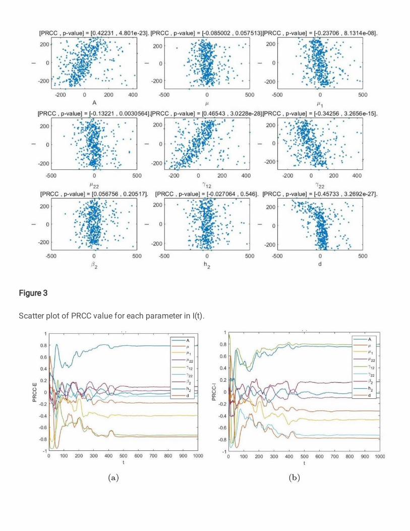
Figure 3
Scatter plot of PRCC value for each parameter in I(t).
Figure 4
PRCC value of each parameter over time.
Figure 5
PRCC values of each parameter in R0.

Figure 6
The disease-free equilibrium point P¯0 is globally asymptotically stable with d = 0.89 which is larger thanthe threshold value 0.8767.
Figure 7
The time-series diagrams for E and I with the different contacting distances while it is larger than thethreshold value 0.8767.
Figure 8
The time-series diagrams for E and I with the different immigration rates while the contacting distance islarger than the threshold value 0.8767.
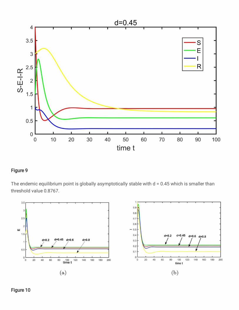
Figure 9
The endemic equilibrium point is globally asymptotically stable with d = 0.45 which is smaller thanthreshold value 0.8767.
Figure 10
The time-series diagrams for E and I with the different contacting distance while it is smaller than thethreshold value 0.8767.
Figure 11
The time-series diagrams for E and I with the different immigration rate while the contacting distance issmaller than the threshold value 0.8767.