Modelling intertidal sediment transport for nutrient change and climate change scenarios

The Science of the Total Environment 314–316(2003) 637–649

0048-9697/03/$ - see front matter� 2003 Elsevier Science B.V. All rights reserved.doi:10.1016/S0048-9697(03)00088-3

Modelling intertidal sediment transport for nutrient change andclimate change scenarios

Rose Wood*, John Widdows

Plymouth Marine Laboratory, Prospect Place, West Hoe, Plymouth PL1 3DH, UK

Received 7 November 2002; accepted 2 January 2003

Abstract

A model of intertidal sediment transport, including effects of bioturbation and biostabilisation, was applied to twotransects on the east coast of England: Leverton(within the Wash) and Skeffling(in the Humber Estuary). Thephysical and biological parameters were chosen to represent four 1-year scenarios: a baseline year(1995), the sameyear but with estuarine nitrate inputs reduced by 50% and by 16%, and a year with climate change effects estimatedfor 2050. The changes in nitrate supply can potentially change microphytobenthos numbers within the surfacesediment, which will then affect erodibility. The model results show a range of behaviour determined by bathymetry,external forcing and biotic state. When intertidal sediment transport is dominated by external sediment supply, themodel produces highest deposition at the most offshore point, and there is greatest deposition in the winter andspring, when offshore sediment concentrations are highest. When intertidal processes dominate intertidal sedimenttransport, there is a peak of deposition at the high-shore level and erosion at mid-tide levels. The greatest depositionnow occurs in winter and summer, when low chlorophyll levels mean that the sediment is most erodible. TheSkeffling transect was dominated by intertidal processes for the baseline scenario and with a 16% reduction in nitrate.Under the climate change(warm winter) scenario, the Skeffling transect was dominated by external sediment supply.The scenario with 50% reduction in nitrate gave intermediate behaviour at Skeffling(intertidally driven during thewinter and summer, and governed by offshore sediment supply during spring and autumn). The Leverton transectwas dominated by offshore sediment supply for all the scenarios.� 2003 Elsevier Science B.V. All rights reserved.

Keywords: Intertidal; Sediment; Transport; Bioturbation; Biostabilisation; Erosion; Deposition

1. Introduction

An abundant benthic community often inhabitsintertidal sand and mudflats. As well as beingimportant from an ecological perspective, biotamay have a large influence on sediment propertiesand behaviour. The effects of biota on sediment

*Corresponding author. Tel.:q44-1752-633100.E-mail address: [email protected](R. Wood).

transport have been summarised and discussed byGraf and Rosenberg(1997). Bioturbators candirectly affect sediment erosion by ejecting mate-rial into the water column, and indirectly affectsediment stability by changing the structure of thebed by loosening it through feeding behaviour, andby changing the nature of bed particles throughingestion and subsequent production of faeces andpseudo-faeces. Both stabilisers and destabilisers

638 R. Wood, J. Widdows / The Science of the Total Environment 314 –316 (2003) 637–649

may also influence the roughness of the sedimentsurface, affecting the bed stress experienced at agiven flow (Wright et al., 1997). Biostabilisers,such as microphytobenthos, can decrease the ero-dibility of sediment by producing extracellularpolysaccharides that bind the sediment(Amos etal., 1998; Sutherland et al., 1998; Austen et al.,1999; de Brouwer et al., 2000; Widdows et al.,2000a). Underwood and Paterson(1993) observedstrong correlation between seasonal changes insurface chlorophylla concentration and sedimentstability. The effects ofMacoma balthica on sedi-ment erodibility have been measured in laboratoryexperiments and field observations(Widdows etal., 1998a,b, 2000b) and subsequently modelled(Willows et al., 1998).

Different types of intertidal flat(Dyer et al.,2000) show different sensitivity to biotic effectson erosion and deposition. The sensitivity is influ-enced by the tidal currents and wave energy theflat experiences, as well as the concentration ofsuspended sediment advected in from the offshoreor long-shore direction and the capacity of the flatto support biota(based largely on the degree ofdisturbance and the percentage of fine sedimentpresent). The role of adjacent intertidal areas assediment suppliers to salt marsh zones has yet tobe quantified. However, changes that affect sedi-ment cycling within the intertidal zone may haveconsequences for morphological change of highershore zones, including saltmarshes, with impactson both habitats and flood and coastal defence.

This work adopts an interdisciplinary approach,whereby the biological effects are parameterisedand used within a hydrodynamic model of sedi-ment transport. The aim of this work was toexamine intertidal sediment transport for four dif-ferent scenarios, using two contrasting model loca-tions. There is a baseline scenario, two scenarioswith altered nutrients, and one scenario withaltered climate. There are major differences in thebiota between the four scenarios and small differ-ences in tidal forcing. The situations that aremodelled represent possible changes in nitratesupply, due to restricting anthropogenic inputs tothe coastal and estuarine systems, and change inclimate. The model is used to explore the possibleresponse of the intertidal sediment system for a

range of changes in the abundance of key biota.Biotic parameters for the different scenarios arepostulated rather than predicted. Therefore, thescenario results show responses to a likely rangeof input parameters, rather than predicting preciseconsequences of change. Reducing nutrient inputwould not be expected to affect a purely physicalmodel of intertidal sediment transport, but byincluding the effects of nutrients on the biota,possible changes can be observed. Similarly, thephysical parameters for climate change(over 50years) used here show only small changes in sealevel and storminess, whereas the effects on theabundance and distribution of the biota over thesame time scale may be large.

2. Conceptual model

Two distinct biological effects on sediment ero-sion are included in the model. Both use relation-ships derived from annular flume experiments,which investigated erosion from sediment with arange of biota density. Velocity was measured atone height(10 cm above the bed). Erosion ratewas related to this velocity and to the number ofclams per unit area of sediment surface.Macomabalthica (small clams), which siphon the surfacesediment during feeding, increase the erosion rateat a given current speed(Willows et al., 1998).When current speeds exceed the critical erosionvelocity (u ), the amount of sediment eroded iscrite

dependent on the density ofMacoma individualspresent. Higher density ofMacoma increases theamount of sediment, which can be eroded at aparticular current speed, until an asymptote isreached. Further increases inMacoma density thenhave no effect on erosion.

A critical erosion speed, at which erosion firstcommences, must be supplied as a model param-eter. Microphytobenthos release polymers(extra-cellular polysaccharide; EPS) in order to propelthemselves as they migrate vertically through thesediment, so that they are at the surface duringdaytime exposure of the tidal flat and lower downat night or during tidal inundation. The EPS itselfis a major stabilising factor in fine sediment(Paterson and Black, 1999). The surface concen-tration of chlorophyll a is an indicator of the

639R. Wood, J. Widdows / The Science of the Total Environment 314 –316 (2003) 637–649

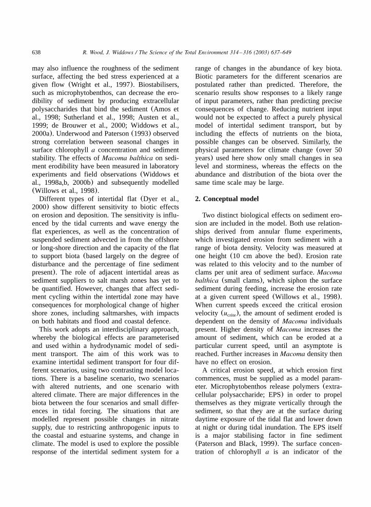
Fig. 1. Locations of the modelled transects on the east coastof England.

amount of EPS present(Underwood and Smith,1998). To incorporate the stabilising effect ofmicrophytobenthos, critical erosion velocity(at 10cm above the bed) is modelled by a linear functionof surface chlorophyll concentration, with para-meters obtained from field data using an annularflume (Widdows et al., 2000a,b).

3. Model description

The model combines a simple 1D model ofcross-shore water movement over an intertidalzone with a semi-empirical model of cohesivesediment erosion and deposition. Each cross-shoretransect is taken as representative of a section ofestuarine shore, which is uniform in the long-shoredirection. Sea surface elevation is supplied to themodel and volume conservation is used to calculatedepth-averaged velocity. These cross-shore veloci-ty values are used to advect water and suspendedsediment using the ECoS modelling system(Gor-ley and Harris, 1998). This functional form is usedwith parameters taken from field experiments atSkeffling. The density ofMacoma individuals andconcentration of chlorophylla within the top 1 cmof surface sediment are specified along the tran-sect. External suspended sediment is imported tothe transect with the flood tide water.

The model has been applied at two locations(Fig. 1). The first transect is at Leverton, on thenorthern shore of the Wash(Fig. 2). Spatial seg-ments are 29.45 m in length. The second transectis at Skeffling on the north shore of the Humber.This transect extends from the shoreline embank-ment to 3.5 km offshore(Fig. 3). Here, eachspatial segment is 35 m in length. Intensive fieldmeasurements have been made at the Skefflingintertidal area and the site is described in Blackand Paterson(1998). The time step is 60 s. Themodel starts from rest, with no suspended sedimentand the tide at low water. Sea surface elevationand suspended sediment concentration are speci-fied at the offshore boundary. The model calculatescurrent speed, suspended sediment concentrationand net sediment mass eroded or deposited withineach segment in the transect. Model runs are madefor single tidal cycles using a variety of boundaryconditions and biota distributions. Results are then

summed appropriately to give budgets of sedimentmovement for sequences of tides.

The model is fully described in Wood andWiddows (2002). The current speed at any timeand place is calculated from conservation of vol-ume, assuming a flat sea surface across the inter-tidal zone, as described in Wood et al.(1998).Sediment transport is then calculated using anadvection–diffusion equation. This is implementedwithin the ECoS modelling package, with diffusioncoefficients set to zero. The numerical scheme isimplicit in time. Sediment erosion rate is deter-mined by current speed andMacoma density(number of 7-mm or longer individuals per m).2

The critical erosion velocity varies with chloro-phyll concentration according to a linear relation-ship, with parameters inferred from experimental


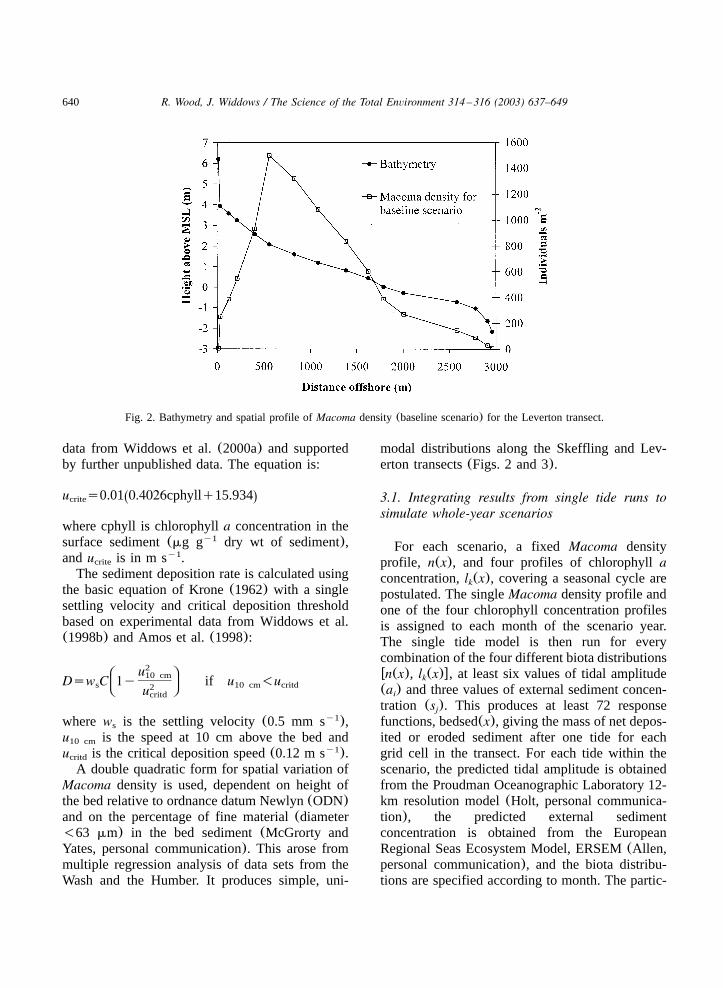
Fig. 2. Bathymetry and spatial profile ofMacoma density(baseline scenario) for the Leverton transect.

data from Widdows et al.(2000a) and supportedby further unpublished data. The equation is:

u s0.010.4026cphyllq15.934Ž .crite

where cphyll is chlorophylla concentration in thesurface sediment(mg g dry wt of sediment),y1

andu is in m s .y1crite

The sediment deposition rate is calculated usingthe basic equation of Krone(1962) with a singlesettling velocity and critical deposition thresholdbased on experimental data from Widdows et al.(1998b) and Amos et al.(1998):

2B Eu10 cmC FDsw C 1y if u -us 10 cm critd2D Gucritd

where w is the settling velocity(0.5 mm s ),y1s

u is the speed at 10 cm above the bed and10 cm

u is the critical deposition speed(0.12 m s ).y1critd

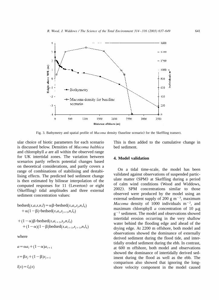
A double quadratic form for spatial variation ofMacoma density is used, dependent on height ofthe bed relative to ordnance datum Newlyn(ODN)and on the percentage of fine material(diameter-63 mm) in the bed sediment(McGrorty andYates, personal communication). This arose frommultiple regression analysis of data sets from theWash and the Humber. It produces simple, uni-

modal distributions along the Skeffling and Lev-erton transects(Figs. 2 and 3).

3.1. Integrating results from single tide runs tosimulate whole-year scenarios

For each scenario, a fixedMacoma densityprofile, n(x), and four profiles of chlorophyllaconcentration,l (x), covering a seasonal cycle arek

postulated. The singleMacoma density profile andone of the four chlorophyll concentration profilesis assigned to each month of the scenario year.The single tide model is then run for everycombination of the four different biota distributionswn(x), l (x)x, at least six values of tidal amplitudek

(a ) and three values of external sediment concen-i

tration (s ). This produces at least 72 responsej

functions, bedsed(x), giving the mass of net depos-ited or eroded sediment after one tide for eachgrid cell in the transect. For each tide within thescenario, the predicted tidal amplitude is obtainedfrom the Proudman Oceanographic Laboratory 12-km resolution model(Holt, personal communica-tion), the predicted external sedimentconcentration is obtained from the EuropeanRegional Seas Ecosystem Model, ERSEM(Allen,personal communication), and the biota distribu-tions are specified according to month. The partic-


Fig. 3. Bathymetry and spatial profile ofMacoma density(baseline scenario) for the Skeffling transect.

ular choice of biotic parameters for each scenariois discussed below. Densities ofMacoma balthicaand chlorophylla are all within the observed rangefor UK intertidal zones. The variation betweenscenarios partly reflects potential changes basedon theoretical considerations, and partly covers arange of combinations of stabilising and destabi-lising effects. The predicted bed sediment changeis then estimated by bilinear interpolation of thecomputed responses for 11(Leverton) or eight(Skeffling) tidal amplitudes and three externalsediment concentration values:

bedsedx,a,s,n,l sabØbedsedx,a ,s ,n,lŽ . Ž .i j k

qa 1yb Øbedsedx,a ,s ,n,lŽ . Ž .i jq1 k

q 1ya bØbedsedx,a ,s ,n,lŽ . Ž .iq1 j k

q 1ya 1yb bedsedx,a ,s ,n,lŽ .Ž . Ž .iq1 jq1 k

where

asaaq 1ya aŽ .i iq1

ssbsq 1yb sŽ .j jq1

l x sl xŽ . Ž .k

This is then added to the cumulative change inbed sediment.

4. Model validation

On a tidal time-scale, the model has beenvalidated against observations of suspended partic-ulate matter(SPM) at Skeffling during a periodof calm wind conditions(Wood and Widdows,2002). SPM concentrations similar to thoseobserved were produced by the model using anexternal sediment supply of 200 g m , maximumy3

Macoma density of 1000 individuals m , andy2

maximum chlorophylla concentration of 10mgg sediment. The model and observations showedy1

intertidal erosion occurring in the very shallowwater behind the flooding edge and ahead of thedrying edge. At 2200 m offshore, both model andobservations showed the dominance of externallyderived sediment during the flood tide, and inter-tidally eroded sediment during the ebb. In contrast,at 600 m offshore, both model and observationsshowed the dominance of intertidally derived sed-iment during the flood as well as the ebb. Thecomparison also showed that ignoring the long-shore velocity component in the model caused


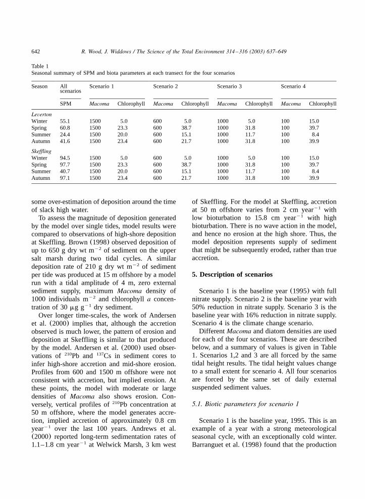
Table 1Seasonal summary of SPM and biota parameters at each transect for the four scenarios

Season All Scenario 1 Scenario 2 Scenario 3 Scenario 4scenarios

SPM Macoma Chlorophyll Macoma Chlorophyll Macoma Chlorophyll Macoma Chlorophyll

LevertonWinter 55.1 1500 5.0 600 5.0 1000 5.0 100 15.0Spring 60.8 1500 23.3 600 38.7 1000 31.8 100 39.7Summer 24.4 1500 20.0 600 15.1 1000 11.7 100 8.4Autumn 41.6 1500 23.4 600 21.7 1000 31.8 100 39.9

SkefflingWinter 94.5 1500 5.0 600 5.0 1000 5.0 100 15.0Spring 97.7 1500 23.3 600 38.7 1000 31.8 100 39.7Summer 40.7 1500 20.0 600 15.1 1000 11.7 100 8.4Autumn 97.1 1500 23.4 600 21.7 1000 31.8 100 39.9

some over-estimation of deposition around the timeof slack high water.

To assess the magnitude of deposition generatedby the model over single tides, model results werecompared to observations of high-shore depositionat Skeffling. Brown(1998) observed deposition ofup to 650 g dry wt m of sediment on the uppery2

salt marsh during two tidal cycles. A similardeposition rate of 210 g dry wt m of sedimenty2

per tide was produced at 15 m offshore by a modelrun with a tidal amplitude of 4 m, zero externalsediment supply, maximumMacoma density of1000 individuals m and chlorophylla concen-y2

tration of 30mg g dry sediment.y1

Over longer time-scales, the work of Andersenet al. (2000) implies that, although the accretionobserved is much lower, the pattern of erosion anddeposition at Skeffling is similar to that producedby the model. Andersen et al.(2000) used obser-vations of Pb and Cs in sediment cores to210 137

infer high-shore accretion and mid-shore erosion.Profiles from 600 and 1500 m offshore were notconsistent with accretion, but implied erosion. Atthese points, the model with moderate or largedensities ofMacoma also shows erosion. Con-versely, vertical profiles of Pb concentration at210

50 m offshore, where the model generates accre-tion, implied accretion of approximately 0.8 cmyear over the last 100 years. Andrews et al.y1

(2000) reported long-term sedimentation rates of1.1–1.8 cm year at Welwick Marsh, 3 km westy1

of Skeffling. For the model at Skeffling, accretionat 50 m offshore varies from 2 cm year withy1

low bioturbation to 15.8 cm year with highy1

bioturbation. There is no wave action in the model,and hence no erosion at the high shore. Thus, themodel deposition represents supply of sedimentthat might be subsequently eroded, rather than trueaccretion.

5. Description of scenarios

Scenario 1 is the baseline year(1995) with fullnitrate supply. Scenario 2 is the baseline year with50% reduction in nitrate supply. Scenario 3 is thebaseline year with 16% reduction in nitrate supply.Scenario 4 is the climate change scenario.

Different Macoma and diatom densities are usedfor each of the four scenarios. These are describedbelow, and a summary of values is given in Table1. Scenarios 1,2 and 3 are all forced by the sametidal height results. The tidal height values changeto a small extent for scenario 4. All four scenariosare forced by the same set of daily externalsuspended sediment values.

5.1. Biotic parameters for scenario 1

Scenario 1 is the baseline year, 1995. This is anexample of a year with a strong meteorologicalseasonal cycle, with an exceptionally cold winter.Barranguet et al.(1998) found that the production


rate of microphytobenthos was strongly influencedby temperature. The influence of cold winter tem-peratures is reflected in low diatom concentrationsduring winter. Beukema et al.(1998) observed arelationship betweenMacoma population and win-ter temperature. Cold winters result in highMaco-ma recruitment during the following summer(dueto changes in fecundity and predator populations).The maximumMacoma density is therefore set ata high value, 1500 individuals m . The densityy2

observed can be much higher than this, but due tothe asymptotic nature of the effect on sedimenterodibility, there will be little difference to theresults if higher values are used.


In scenario 2, tidal forcing is the same as forthe baseline year, but there is a 50% reduction innitrate supply to the estuaries. Beukema and Cadee(1997) showed that zoobenthos biomass doubledfollowing a doubling of phytoplankton biomass inthe Wadden Sea, believed to be due to increasednutrient supply. If so, it is plausible that a subse-quent halving in nitrate input might lead to asignificant decrease in zoobenthos. Thus, for thisscenario, the maximumMacoma density is reducedto 600 individuals m . Peletier(1996) observedy2

that during years with lower nutrient supply, therewere microphytobenthos blooms on an estuarinemudflat during spring and autumn, whereas inyears with greater nutrient supply, there was lessseasonal variation in surface chlorophyll. Thus, toreflect the reduced nutrients, diatoms(and hencechlorophyll a concentration) are given a higherspring peak due to lower grazing, and only a smallautumn peak.


In scenario 3, tidal forcing is the same as forthe baseline year, but there is a 16% reduction innitrate supply to the estuaries. This scenario isintermediate between scenarios 1 and 2. There islittle evidence that microphytobenthos orMacomaare currently nutrient-limited, but decreases inorganic matter, which might be associated withreductions in nitrate supply, could result in lower

Macoma numbers. The maximumMacoma densityis set at 1000 individuals m . The distribution ofy2

diatoms imposed has strong peaks in the springand the autumn, consistent with predation byMacoma cutting off the spring peak and recyclingnutrients, which then support the autumn bloom.

5.4. Biota parameters for scenario 4

This is the climate-change scenario. The condi-tions for the mid-21st century climate(sea levelraised by 28 cm, annual air temperature increasedby 1.5–3.2 8C in England, reduced temperaturevariability in winter, increased variability in sum-mer) are based on Hume and Jenkins(1998).Warm winters are associated with lowMacomarecruitment. The maximumMacoma density is setto 100 individuals m because of the highery2

winter temperatures. Peak diatom density is sethigh because of the lower grazing byMacoma,but with low summer values due to desiccationassociated with high summer temperatures.

Table 1 shows the average seasonal values forMacoma density, chlorophylla concentration andexternal SPM concentration for each of the modelscenarios, for each transect. Scenarios 1 and 3have highMacoma density and a similar range ofchlorophyll values. Scenarios 2 and 4 have higherchlorophylla values during the spring and autumn,and lower Macoma numbers. The transects atLeverton and Skeffling are subject to the samespatial maximum values forMacoma and chloro-phyll a, but the daily values of external SPMsupplied are different, although both show a strongseasonal component.

6. Results

6.1. Seasonal response

For every tidal cycle within each scenario year,the model produces the net deposition(or erosion)at each grid cell along the transect. These havebeen summed for 3-month periods to split theoverall response into seasonal components. Tidalcurrents during neap tides are generally below thecritical erosion speed, so erosion of intertidalsediment primarily occurs on spring tides. For


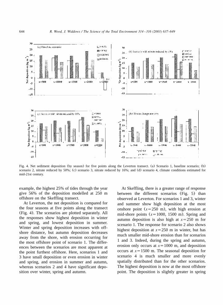
Fig. 4. Net sediment deposition(by season) for five points along the Leverton transect.(a) Scenario 1, baseline scenario;(b)scenario 2, nitrate reduced by 50%;(c) scenario 3, nitrate reduced by 16%; and(d) scenario 4, climate conditions estimated formid-21st century.

example, the highest 25% of tides through the yeargive 56% of the deposition modelled at 250 moffshore on the Skeffling transect.

At Leverton, the net deposition is compared forthe four seasons at five points along the transect(Fig. 4). The scenarios are plotted separately. Allthe responses show highest deposition in winterand spring, and lowest deposition in summer.Winter and spring deposition increases with off-shore distance, but autumn deposition decreasesaway from the shore, with erosion occurring forthe most offshore point of scenario 1. The differ-ences between the scenarios are most apparent atthe point furthest offshore. Here, scenarios 1 and3 have small deposition or even erosion in winterand spring, and erosion in summer and autumn,whereas scenarios 2 and 4 have significant depo-sition over winter, spring and autumn.

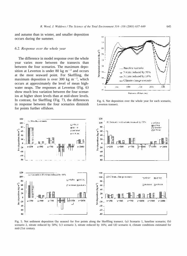
At Skeffling, there is a greater range of responsebetween the different scenarios(Fig. 5) thanobserved at Leverton. For scenarios 1 and 3, winterand summer show high deposition at the mostonshore point(xs250 m), with high erosion atmid-shore points(xs1000, 1500 m). Spring andautumn deposition is also high atxs250 m forscenario 1. The response for scenario 2 also showshighest deposition atxs250 m in winter, but hasmuch smaller mid-shore erosion than for scenarios1 and 3. Indeed, during the spring and autumn,erosion only occurs atxs1000 m, and depositionoccurs atxs1500 m. The seasonal deposition forscenario 4 is much smaller and more evenlyspatially distributed than for the other scenarios.The highest deposition is now at the most offshorepoint. The deposition is slightly greater in spring


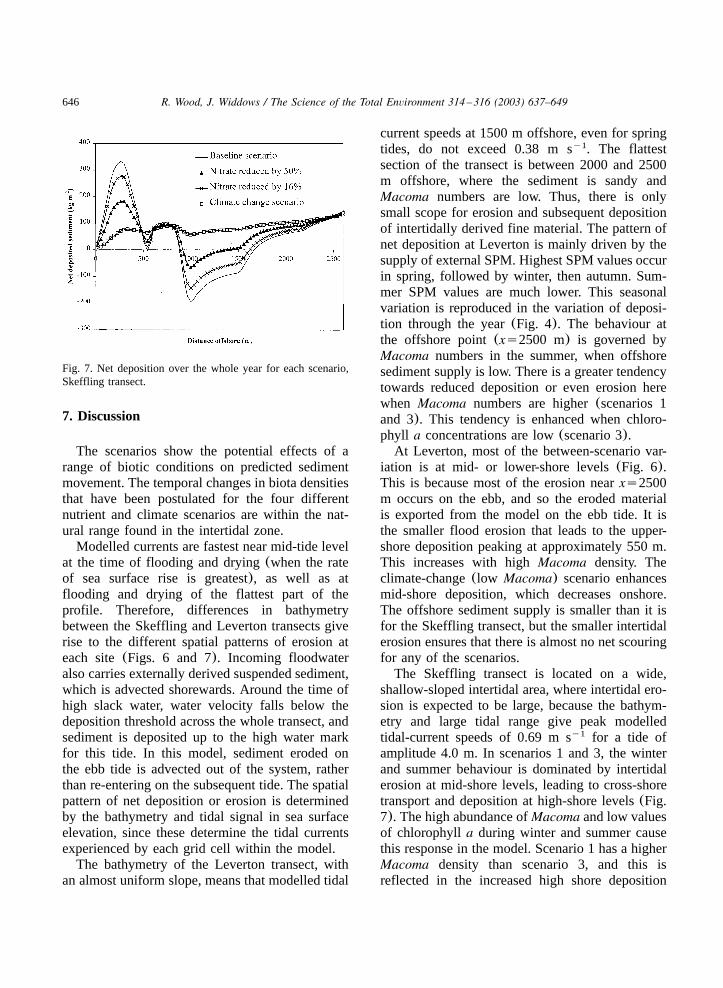
Fig. 6. Net deposition over the whole year for each scenario,Leverton transect.

Fig. 5. Net sediment deposition(by season) for five points along the Skeffling transect.(a) Scenario 1, baseline scenario;(b)scenario 2, nitrate reduced by 50%;(c) scenario 3, nitrate reduced by 16%; and(d) scenario 4, climate conditions estimated formid-21st century.

and autumn than in winter, and smaller depositionoccurs during the summer.

6.2. Response over the whole year

The difference in model response over the wholeyear varies more between the transects thanbetween the four scenarios. The maximum depo-sition at Leverton is under 80 kg m and occursy2

at the most seaward point. For Skeffling, themaximum deposition is over 300 kg m , whichy2

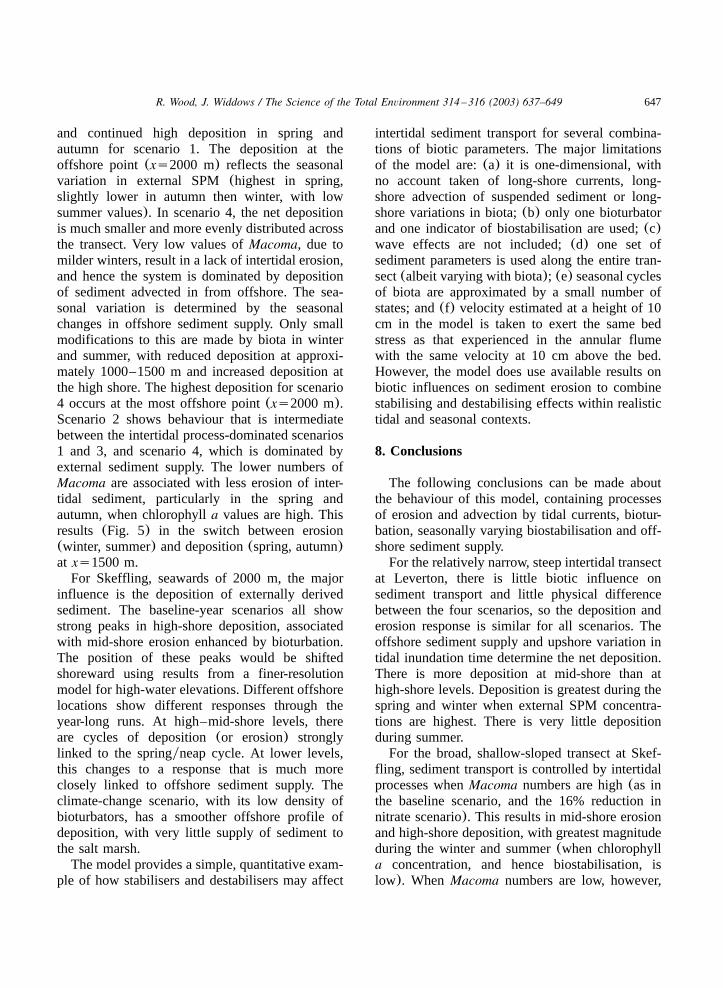
occurs at approximately the level of mean high-water neaps. The responses at Leverton(Fig. 6)show much less variation between the four scenar-ios at higher shore levels than at mid-shore levels.In contrast, for Skeffling(Fig. 7), the differencesin response between the four scenarios diminishfor points further offshore.


Fig. 7. Net deposition over the whole year for each scenario,Skeffling transect.

7. Discussion

The scenarios show the potential effects of arange of biotic conditions on predicted sedimentmovement. The temporal changes in biota densitiesthat have been postulated for the four differentnutrient and climate scenarios are within the nat-ural range found in the intertidal zone.

Modelled currents are fastest near mid-tide levelat the time of flooding and drying(when the rateof sea surface rise is greatest), as well as atflooding and drying of the flattest part of theprofile. Therefore, differences in bathymetrybetween the Skeffling and Leverton transects giverise to the different spatial patterns of erosion ateach site(Figs. 6 and 7). Incoming floodwateralso carries externally derived suspended sediment,which is advected shorewards. Around the time ofhigh slack water, water velocity falls below thedeposition threshold across the whole transect, andsediment is deposited up to the high water markfor this tide. In this model, sediment eroded onthe ebb tide is advected out of the system, ratherthan re-entering on the subsequent tide. The spatialpattern of net deposition or erosion is determinedby the bathymetry and tidal signal in sea surfaceelevation, since these determine the tidal currentsexperienced by each grid cell within the model.

The bathymetry of the Leverton transect, withan almost uniform slope, means that modelled tidal

current speeds at 1500 m offshore, even for springtides, do not exceed 0.38 m s . The flattesty1

section of the transect is between 2000 and 2500m offshore, where the sediment is sandy andMacoma numbers are low. Thus, there is onlysmall scope for erosion and subsequent depositionof intertidally derived fine material. The pattern ofnet deposition at Leverton is mainly driven by thesupply of external SPM. Highest SPM values occurin spring, followed by winter, then autumn. Sum-mer SPM values are much lower. This seasonalvariation is reproduced in the variation of deposi-tion through the year(Fig. 4). The behaviour atthe offshore point(xs2500 m) is governed byMacoma numbers in the summer, when offshoresediment supply is low. There is a greater tendencytowards reduced deposition or even erosion herewhen Macoma numbers are higher(scenarios 1and 3). This tendency is enhanced when chloro-phyll a concentrations are low(scenario 3).

At Leverton, most of the between-scenario var-iation is at mid- or lower-shore levels(Fig. 6).This is because most of the erosion nearxs2500m occurs on the ebb, and so the eroded materialis exported from the model on the ebb tide. It isthe smaller flood erosion that leads to the upper-shore deposition peaking at approximately 550 m.This increases with highMacoma density. Theclimate-change(low Macoma) scenario enhancesmid-shore deposition, which decreases onshore.The offshore sediment supply is smaller than it isfor the Skeffling transect, but the smaller intertidalerosion ensures that there is almost no net scouringfor any of the scenarios.

The Skeffling transect is located on a wide,shallow-sloped intertidal area, where intertidal ero-sion is expected to be large, because the bathym-etry and large tidal range give peak modelledtidal-current speeds of 0.69 m s for a tide ofy1

amplitude 4.0 m. In scenarios 1 and 3, the winterand summer behaviour is dominated by intertidalerosion at mid-shore levels, leading to cross-shoretransport and deposition at high-shore levels(Fig.7). The high abundance ofMacoma and low valuesof chlorophyll a during winter and summer causethis response in the model. Scenario 1 has a higherMacoma density than scenario 3, and this isreflected in the increased high shore deposition


and continued high deposition in spring andautumn for scenario 1. The deposition at theoffshore point(xs2000 m) reflects the seasonalvariation in external SPM(highest in spring,slightly lower in autumn then winter, with lowsummer values). In scenario 4, the net depositionis much smaller and more evenly distributed acrossthe transect. Very low values ofMacoma, due tomilder winters, result in a lack of intertidal erosion,and hence the system is dominated by depositionof sediment advected in from offshore. The sea-sonal variation is determined by the seasonalchanges in offshore sediment supply. Only smallmodifications to this are made by biota in winterand summer, with reduced deposition at approxi-mately 1000–1500 m and increased deposition atthe high shore. The highest deposition for scenario4 occurs at the most offshore point(xs2000 m).Scenario 2 shows behaviour that is intermediatebetween the intertidal process-dominated scenarios1 and 3, and scenario 4, which is dominated byexternal sediment supply. The lower numbers ofMacoma are associated with less erosion of inter-tidal sediment, particularly in the spring andautumn, when chlorophylla values are high. Thisresults (Fig. 5) in the switch between erosion(winter, summer) and deposition(spring, autumn)at xs1500 m.

For Skeffling, seawards of 2000 m, the majorinfluence is the deposition of externally derivedsediment. The baseline-year scenarios all showstrong peaks in high-shore deposition, associatedwith mid-shore erosion enhanced by bioturbation.The position of these peaks would be shiftedshoreward using results from a finer-resolutionmodel for high-water elevations. Different offshorelocations show different responses through theyear-long runs. At high–mid-shore levels, thereare cycles of deposition(or erosion) stronglylinked to the springyneap cycle. At lower levels,this changes to a response that is much moreclosely linked to offshore sediment supply. Theclimate-change scenario, with its low density ofbioturbators, has a smoother offshore profile ofdeposition, with very little supply of sediment tothe salt marsh.

The model provides a simple, quantitative exam-ple of how stabilisers and destabilisers may affect

intertidal sediment transport for several combina-tions of biotic parameters. The major limitationsof the model are:(a) it is one-dimensional, withno account taken of long-shore currents, long-shore advection of suspended sediment or long-shore variations in biota;(b) only one bioturbatorand one indicator of biostabilisation are used;(c)wave effects are not included;(d) one set ofsediment parameters is used along the entire tran-sect(albeit varying with biota); (e) seasonal cyclesof biota are approximated by a small number ofstates; and(f) velocity estimated at a height of 10cm in the model is taken to exert the same bedstress as that experienced in the annular flumewith the same velocity at 10 cm above the bed.However, the model does use available results onbiotic influences on sediment erosion to combinestabilising and destabilising effects within realistictidal and seasonal contexts.

8. Conclusions

The following conclusions can be made aboutthe behaviour of this model, containing processesof erosion and advection by tidal currents, biotur-bation, seasonally varying biostabilisation and off-shore sediment supply.

For the relatively narrow, steep intertidal transectat Leverton, there is little biotic influence onsediment transport and little physical differencebetween the four scenarios, so the deposition anderosion response is similar for all scenarios. Theoffshore sediment supply and upshore variation intidal inundation time determine the net deposition.There is more deposition at mid-shore than athigh-shore levels. Deposition is greatest during thespring and winter when external SPM concentra-tions are highest. There is very little depositionduring summer.

For the broad, shallow-sloped transect at Skef-fling, sediment transport is controlled by intertidalprocesses whenMacoma numbers are high(as inthe baseline scenario, and the 16% reduction innitrate scenario). This results in mid-shore erosionand high-shore deposition, with greatest magnitudeduring the winter and summer(when chlorophylla concentration, and hence biostabilisation, islow). When Macoma numbers are low, however,


as in the climate-change scenario, sediment trans-port becomes dominated by the external sedimentsupply. Deposition increases offshore and variesseasonally according to offshore SPM concentra-tion. For moderateMacoma density(as in the 50%reduction in nitrate scenario), the intertidal pro-cesses dominate during winter and summer, andthe external sediment supply dominates duringspring and autumn.

Acknowledgments

The authors would like to thank Ruth Cox andMick Yates of the Centre for Ecology and Hydrol-ogy, Monkswood, UK, and John Goss-Custard andSelwyn McGrorty of the Centre for Ecology andHydrology, Wareham for their contributions to thework. This work was carried out as part of Objec-tive 4 of the NERC Land–Ocean Interaction Study(LOIS) program, and DEFRA contract numberAE0259.

References

Amos CL, Brylinsky M, Sutherland TF, O’Brien D, Lee S,Cramp A. The stability of a mudflat in the Humber estuary,South Yorkshire, UK. In: Black KS, Paterson DM, CrampA, editors. Sedimentary processes in the intertidal zone.Special Publication 139. London: Geological Society, 1998.p. 25–44.

Andersen TJ, Mikkelsen OA, Moller AL, Pejrup M. Depositionand mixing depths on some European intertidal mudflatsbased on Pb-210 and Cs-137 activities. Continental ShelfRes 2000;20:1569–1591.

Andrews JE, Samways G, Dennis PF, Maher BA. Origin,abundance and storage of organic carbon and sulfur in theHolocene Humber Estuary—emphasising human impact onstorage changes. In: Shennan I, Andrews JE, editors. Holo-cene land–ocean interaction and environmental changearound the western North Sea. Special Publication 166.London: Geological Society, 2000. p. 145–170.

Austen I, Andersen TJ, Edelvang K. The influence of benthicdiatoms and invertebrates on the erodibility of an intertidalmud flat. Estuarine Coastal Shelf Sci 1999;49:99–111.

Barranguet C, Kromkamp J, Peene J. Factors controllingprimary production and photosynthetic characteristics ofintertidal microphytobenthos. Mar Ecol Prog Ser1998;173:117–126.

Beukema JJ, Cadee GC. Local differences in macrozoobenthicresponse to enhanced food supply caused by mild eutro-phication in a Wadden Sea area: food is only locally alimiting factor. Limnol Oceanogr 1997;42:1424–1435.

Beukema JJ, Honkoop OJC, Dekker R. Recruitment inMaco-ma balthica after mild and cold winters and its possiblecontrol by egg production and shrimp predation. Hydrobiol-ogia 1998;376:23–34.

Black KS, Paterson DM. LISP-UK. Littoral investigation ofsediment properties: an introduction. In: Black KS, PatersonDM, Cramp A, editors. Sedimentary processes in the inter-tidal zone. Special Publication 139. London: GeologicalSociety, 1998. p. 1–10.

de Brouwer JFC, Bjelic S, de Deckere EMGT, Stal LJ.Interplay between biology and sedimentology in a mudflat(Biezelingse Ham, Westerschelde, The Netherlands). Con-tinental Shelf Res 2000;20:1159–1177.

Brown SL. Sedimentation on a Humber salt marsh. In: BlackKS, Paterson DM, Cramp A, editors. Sedimentary processesin the intertidal zone. Special Publication 139. London:Geological Society, 1998. p. 69–84.

Dyer KR, Christie MC, Wright EW. The classification ofintertidal mudflats. Continental Shelf Res 2000;20:1039–1060.

Gorley RN, Harris JRW. ECoS3 user guide. Swindon, UK:Plymouth Marine Laboratory, Natural Environment ResearchCouncil, 1998. (35 pp).

Graf G, Rosenberg R. Bioresuspension and biodeposition: areview. J Mar Syst 1997;11(3–4):269–278.

Hume M, Jenkins GJ. Climate change scenarios for the UK:Scientific report. UKCIP Technical Report No 1. Norwich:Climate Research Unit, 1998. (80 pp).

Krone RB. Flume studies of the transport of sediment inestuarial shoaling processes. Berkeley, CA: University ofCalifornia, Hydraulics Engineering Laboratory and SaintEngineering Laboratory, 1962. (110 pp).

Paterson DM, Black KS. Water flow, sediment dynamics, andbenthic biology. In: Raffaelli D, Nedwell D, editors.Advances in ecological research, vol. 29. Oxford UniversityPress, 1999. p. 155–193.

Peletier H. Long-term changes in intertidal estuarine diatomassemblages related to reduced input of organic waste. MarEcol Progr Ser 1996;137:265–271.

Sutherland TF, Grant J, Amos CL. The effect of carbohydrateproduction by the diatomNitzschia curvilineata on theerodibility of sediment. Limnol Oceanogr 1998;43:65–72.

Underwood GJC, Paterson DM. Seasonal changes in diatombiomass, sediment stability and biogenic stabilisation in theSevern Estuary. J Mar Biol Assoc 1993;73:871–887.

Underwood GJC, Smith DJ. Predicting epipelic diatom exo-polymer concentrations in intertidal sediments from sedi-ment chlorophylla. Microb Ecol 1998;35:116–125.

Widdows J, Brinsley MD, Salkeld PN, Elliott M. Use ofannular flumes to determine the influence of current velocityand bivalves on material flux at the sediment–water inter-face. Estuaries 1998;21:552–559.

Widdows J, Brinsley M, Elliott M. Use of an in situ flume toquantify particle flux (biodeposition rates and sedimenterosion) for an intertidal mudflat in relation to changes in


current velocity and benthic macrofauna. In: Black KS,Paterson DM, Cramp A, editors. Sedimentary processes inthe intertidal zone. Special Publication 139. London: Geo-logical Society, 1998. p. 85–98.

Widdows J, Brinsley MD, Salkeld PN, Lucas C. Influence ofbiota on spatial and temporal variation in sediment erodi-bility and material flux on a tidal flat(Westerschelde, TheNetherlands). Mar Ecol Prog Ser 2000;194:23–27.

Widdows J, Brown S, Brinsley MD, Salkeld PN, Elliott M.Temporal changes in intertidal sediment erodibility: influ-ence of biological and climatic factors. Continental ShelfRes 2000;20:1275–1290.

Willows RI, Widdows J, Wood RG. Influence of an infaunalbivalve on the erosion of an intertidal cohesive sediment: a

flume and modelling study. Limnol Oceanogr1998;43:1332–1343.

Wood RG, Black KS, Jago CF. Measurements and preliminarymodelling of current velocity over an intertidal mudflat,Humber estuary, UK. In: Black KS, Paterson DM, CrampA, editors. Sedimentary processes in the intertidal zone.Special Publication 139. London: Geological Society, 1998.p. 167–176.

Wood RG, Widdows J. A model of sediment transport overan intertidal transect, comparing the influences of biologicaland physical factors. Limnol Oceanogr 2002;47:848–855.

Wright LD, Schaffner LC, Maa JPY. Biological mediation ofbottom boundary layer processes and sediment suspensionin the lower Chesapeake Bay. Mar Geol 1997;141:27–50.

Documents

Modelling intertidal sediment transport for nutrient change and climate change scenarios