Thesis Biobased Chemistry and Technology

Biobased Chemistry and Technology

Modelling of a Dutch agricultural region containing grass and maize biorefineries

Niels de Beus

07-05-2015

Modelling of a Dutch agricultural region containing grass and maize biorefineries

Name course : Thesis project Biobased Chemistry and Technology

Number : BCT-80436 Study load : 36 ects Date : 07-05-2015 Student : Niels de Beus Registration number : 910618063030 Study programme : MBT (Biotechnology) Report number : 018BCT Supervisor(s) : A.M. Teekens and L.G. van Willigenburg Examiners : Dr. ir. A.J.B. van Boxtel Group : Biobased Chemistry and Technology Address : Bornse Weilanden 9 6708 WG Wageningen the Netherlands Tel: +31 (317) 48 21 24 Fax: +31 (317) 48 49 57

Abstract This study focuses on the design of an agricultural region containing 7 blocks; grass farm, maize

farm, grass biorefinery, maize biorefinery, pig farm, cattle farm and an anaerobic fermenter. The agricultural region contains 20000 dairy cattle and 100000 pigs. Mass balances are used to describe the relations between inputs and outputs of a single block. All blocks are connected afterwards to create a nutrient recycling agricultural region.

The grass biorefinery separates the grass into a protein product, a fibre product, an animal feed

product and the left over juice. The protein product contains little fibre which enables pigs to consume the proteins in grass. Another benefit is the reduction of P and K in the feed products. The maize biorefinery produces an animal feed product, a fibre product, a nutrient rich juice and ethanol. The juices

in the biorefinery can be recycled to the agricultural soil. The anaerobic fermenter ferments manure and fibres not fed to the cattle, the resulting products are biogas and digestate. The digestate contains valuable nutrients and residual organic matter. By recycling the digestate back to the agricultural land nutrients are used more efficient and the soil is enhanced in organic matter.

The model of the agricultural region contains 23 decision variables; 8 related to import of feed and

fertilizer, 5 related to the opening and closing the cycle and 10 related to the distribution of produce in the region. The model contains 5 equality constrains to ensure the region is cyclic, 4 equality constraints to satisfy energy and protein demand of the pigs and cattle and 1 equality constraint related to the distribution of maize over the three potential desinations.

The region is optimised with different objective functions. The objective of one of the optimisation is to maximise profit in the region and minimize area of land use. An increasing weighing factor on area of land use is used to create a series of optimisations. It was found that imposing a land use penalty reduces the system size from 18000 ha to 9000 ha. Total profit decreased as the weighing factor increased, from 60 to 45 million euro. Other findings of this series include a decrease of self-sufficiency in smaller regions. The P excretion increased in smaller regions. This makes the model valuable for policy evaluation and land use change analysis.

Given the increase of P excretion in the land use series, a second series of optimisations was

performed. The objective function of this series included a maximisation of total profit and a minimisation of P excretion. The series is created by increasing the weighing factor on P excretion. To prevent the region from increasing the area of land use, a maximum area of land use is used in this series. The

maximum is set at 15000 ha. As the weighing factor on P excretion increased, P excretion decreased while total profit did not decrease. The P excretion for pigs was reduced with 30 ton P per year. The reduction in P excrtion is attributed to a change in diet composition for pigs. As the penalty increases, imported feed is replaced by refined feed, which contains less P. The reduction of P excretion helps to reduce the manure excess in the Netherlands. This series shows that the model can also be used to analyse the effect of environmental policies.

A separate model has been created to simulate the organic matter in the agricultural soils. From this

model it is concluded that the organic matter in the digestate contributes to the soil organic matter. Only applying the residual organic matter reduces the soil organic matter. When the root systems of the crops are also taken into account, the soil organic matter remains stable.

Seven regions are discussed in more detail to get better understanding of the agricultural regions. It is shown that the optimisation can produce very different regions. Each of the regions has advantages over the other regions, but also disadvantages. The implementation of the designed region is complex because it involves many different stakeholders with different goals. The model created in this study is valuable in the design of the agricultural region because it can simulate different scenarios and objectives. However for the implementation of the proposed region there needs to be consent amog stakeholders over the goals and constraints of the region.

From the results is is concluded that a model is created which can design an agricultural region when

given an objective function with a set of constraints. The ability to include various policy instruments makes it a valuable tool for stakeholders in the region. The model can also be used to predict land use

change in agricultural regions and determine the self-sufficiecy. These are interesting properties for the global land use discussion and food security issues.

1

2

Contents List of Figures ............................................................................................................................ 4

List of Tables ............................................................................................................................. 5

1. Introduction .......................................................................................................................... 6

1.1 Aim and approach .............................................................................................................. 6

2. The agricultural system ........................................................................................................... 8

2.1 Soil .................................................................................................................................. 8

2.1.1 Nutrients in the soil ...................................................................................................... 9

2.1.2 Soil organic matter model .............................................................................................. 9

2.2 Maize farm ...................................................................................................................... 10

2.3 Grass farm ...................................................................................................................... 11

2.4 Crop rotation ................................................................................................................... 12

2.5 Small scale biorefinery ...................................................................................................... 13

2.5.1 Grass biorefinery ........................................................................................................ 13

2.5.2 Maize biorefinery ........................................................................................................ 14

2.6 Livestock ........................................................................................................................ 15

2.6.1 Dairy farm ................................................................................................................. 15

2.6.2 Pig farm .................................................................................................................... 15

2.7 Anaerobic fermentation ..................................................................................................... 16

2.7.1 The anaerobic fermenter model .................................................................................... 17

2.7.2 Estimating H2S concentration in the biogas..................................................................... 18

2.7.3 Digestate .................................................................................................................. 18

2.10 Dutch fertilizer law ......................................................................................................... 18

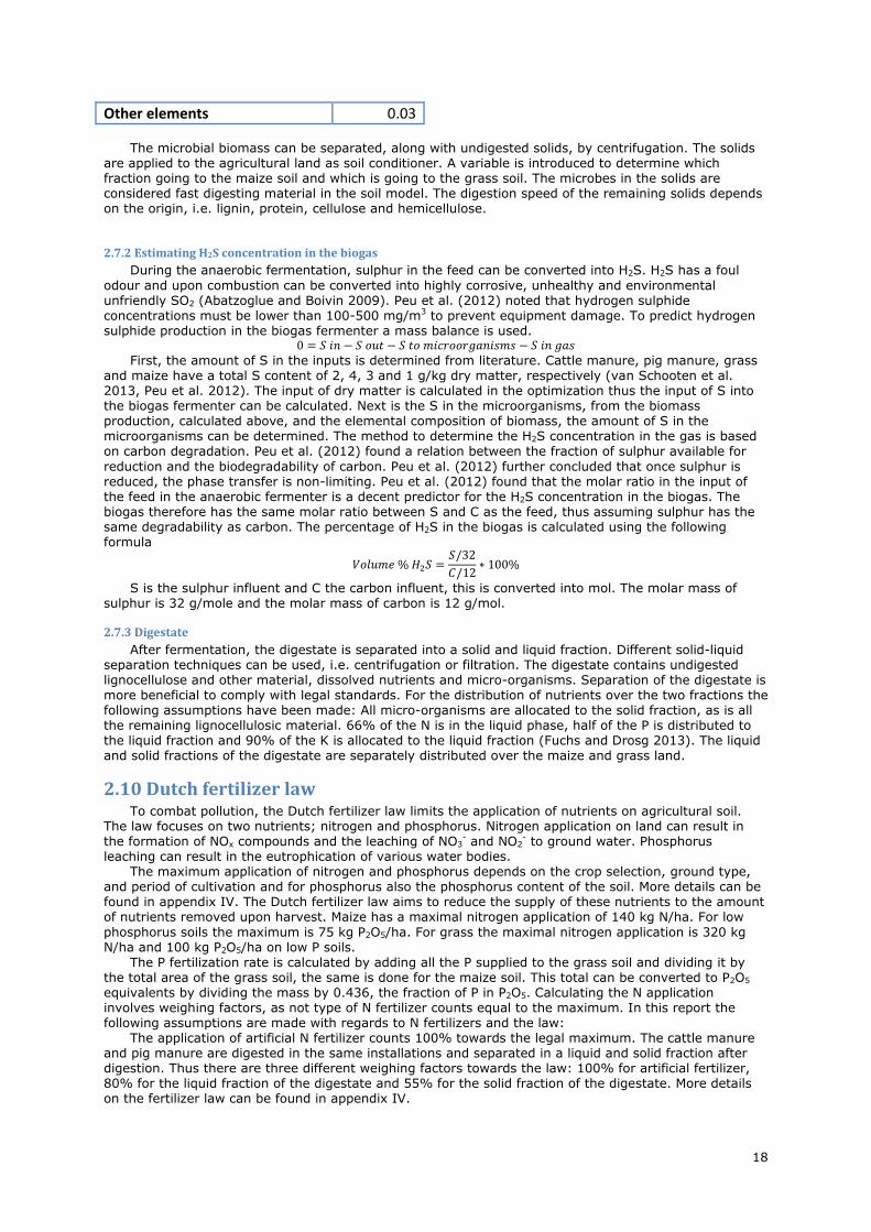
3. Optimisation ........................................................................................................................ 20

3.1 Decision variables and constraints ...................................................................................... 20

3.2 Objective function ............................................................................................................ 21

3.3 Initial guesses ................................................................................................................. 22

4. Results ............................................................................................................................... 24

4.1 Land use series ............................................................................................................... 24

4.1.1 Total profit and land use .............................................................................................. 24

4.1.2 Import in the agricultural region ................................................................................... 25

4.1.3 Phosphorus excretion .................................................................................................. 26

4.1.4 Biorefineries .............................................................................................................. 27

4.1.5 Soil organic matter ..................................................................................................... 28

4.1.6 Crop rotation in the agricultural region .......................................................................... 30

4.2 P excretion series ............................................................................................................ 31

4.2.1 Total profit and P excretion .......................................................................................... 31

4.2.2 Land use and import ................................................................................................... 33

4.2.3 Biorefineries .............................................................................................................. 34

4.2.4 Soil organic matter ..................................................................................................... 35

4.3 Individual systems ........................................................................................................... 35

3

5. Discussion ........................................................................................................................... 42

5.1 Maize distribution............................................................................................................. 42

5.2 Area of land use .............................................................................................................. 42

5.3 Biorefineries .................................................................................................................... 43

5.4 Soil organic matter .......................................................................................................... 44

5.5 Biological nitrogen fixation ................................................................................................ 44

6. Conclusions ......................................................................................................................... 46

7. Recommendations ................................................................................................................ 48

8. Acknowledgement ................................................................................................................ 49

9. Reference ........................................................................................................................... 50

Appendix I. Calculation energy and protein requirement for cows .................................................... 56

Appendix II. Calculation energy and protein requirement for pigs .................................................... 57

Appendix III. Calculation of lignocellulose digestibility ................................................................... 58

Appendix IV. Dutch fertilization law ............................................................................................ 59

Appendix V. Replacing imported feed with refined rapeseed ........................................................... 62

Appendix VI. Prices for commodities ........................................................................................... 63

Appendix VII. The mathematical model. ...................................................................................... 64

4

List of Figures Figure 1, schematic overview of the blocks in the agricultural region and the links between the blocks. .. 7 Figure 2, schematic overview of a single block. ............................................................................... 7 Figure 3, schematic overview of Soil organic matter model. .............................................................. 9 Figure 4, schematic overview of the mass flow in the Grassa process (Melkvee 2014). ....................... 13 Figure 5, schematic overview of the agricultural region, links between the blocks and the different mass

flows. ..................................................................................................................................... 20 Figure 6, objective function, total profit and area of land use plotted against the weighing factor ......... 24 Figure 7, individual total profit (left) and area of land use (right) plotted against the land use penalty. . 25 Figure 8, total profit per hectare plotted against the land use penalty (left) and area of land use (right).

............................................................................................................................................. 25 Figure 9, total profit and total import plotted against land use penalty and area of land use ................ 25 Figure 10, imported feed and fertilizer plotted against the penalty on land use .................................. 26 Figure 11, P excretion plotted against area of land use. ................................................................. 26 Figure 12, diet composition of pigs (left) and cattle (right) plotted against area of land use.

(Optimisations 13 to 18 are all around 9200 ha) ........................................................................... 27 Figure 13, biorefinery profit plotted against land use penalty. ......................................................... 27 Figure 14, profit (left) and mass input (right) of the individual biorefineries. ..................................... 28 Figure 15, equilibrium soil organic matter in a 2:1 grass: maize rotation. ......................................... 28 Figure 16, soil organic matter development over 3 years. .............................................................. 29 Figure 17, soil organic matter dynamics over 30 years. ................................................................. 29 Figure 18, soil organic matter dynamics over 300 years. ................................................................ 30 Figure 19, percentage of grass and maize land in the agricultural region. ......................................... 31 Figure 20, objective function value, total profit and total P excretion of the P excretion series. (With total

P excretion on the secondary y-axis)........................................................................................... 32 Figure 21, total P excretion (left) and total profit (right) of the P excretion series. ............................. 32 Figure 22, P excretion (left) and diet composition of cattle in the P excretion series. .......................... 32 Figure 23, diet composition of the pigs in the P excretion series. ..................................................... 33 Figure 24, Area of land use in the P excretion series. ..................................................................... 33 Figure 25, Total profit and imports in the P excretion series. (With imports on the secondary y-axis) .... 34 Figure 26, mass refined (left) and profit (right) of the biorefineries in the agricultural region. .............. 34 Figure 27, equilibrium soil organic matter in the agricultural region. ................................................ 35 Figure 28, profit of the blocks in the region .................................................................................. 38 Figure 29, total area of land use of the agricultural regions in the land use series. ............................. 43

5

List of Tables Table 1, chemical composition of maize ....................................................................................... 11 Table 2, chemical composition of grass ........................................................................................ 12 Table 3, fractionation of different component in the Grassa biorefinery process ................................. 14 Table 4, fractionation of different component in the maize biorefinery process. ................................. 14 Table 5, inputs and outputs of dairy cows related to amount of product. .......................................... 15 Table 6, inputs and outputs of pigs related to the amount of product ............................................... 16 Table 7, typical composition of bacteria cells ................................................................................ 17 Table 8, list of decision variables in the agricultural system, their units and the upper and lower bounds

............................................................................................................................................. 21 Table 9, optimisation number and corresponding land use penalty................................................... 24 Table 10 , optimisation numbers and corresponding P excretion penalty. .......................................... 31 Table 11, total profit, imports and areas of seven agricultural regions .............................................. 36 Table 12, fertilization rates and manure excess. ........................................................................... 37 Table 13, profit per block. ......................................................................................................... 37 Table 14, P excretion ................................................................................................................ 38 Table 15, distribution of refined produce. ..................................................................................... 39 Table 16, Biological nitrogen fixation and yield limiting nutrient for grass. ........................................ 39 Table 17, equilibrium of soil organic matter.................................................................................. 39 Table 18, anaerobic fermenter performance. ................................................................................ 40 Table 19, whole maize plant composition compared with corn cob mix composition. ........................... 42 Table 20, feed regime for meat pigs............................................................................................ 57 Table 21 Energy and protein requirements for pigs (CVB 2008) ...................................................... 57 Table 22 lignocellulosic materials in manure of dairy cattle and pigs ................................................ 58 Table 23, calculation of the digestibility of lignocellulosic materials by dairy cattle and pigs ................. 58 Table 24, maximum N fertilization rate of different crops on soils in the Netherlands. ......................... 59 Table 25, maximum P2O5 fertilization rate on soils in the Netherlands. ............................................. 59 Table 26, weighing factors of materials in the Dutch fertilizer law. ................................................... 60 Table 27, different weighing methods possible in the agricultural region. .......................................... 61 Table 28, composition of refined rapeseed ................................................................................... 62 Table 29, prices of commodities ................................................................................................. 63

6

1. Introduction Agriculture, the domestication of plants and animals, has been known to mankind for centuries.

Cultivation techniques as crop rotation, irrigation and fertilization were developed to stabilize and increase crop yield. A major breakthrough in agriculture was the development of the Haber-Bosch process to produce NH3 from N2 and H2 (Smil 2001). The Haber-Bosch process allowed humans to synthesize fertilizers. Application of fertilizer on agricultural land increased the often limiting N supply to crops. With this restriction lifted, crop yield increased significantly. Implementation of more recent technological advances in the last 50-75 years led to a substantial increase in global food production (Alexandratos and Bruinsma 2012). By separation and specialization, agricultural practices intensified; resulting in monocultures, which reduce agrobiodeversity, and mega-farms, including intensive animal farming.

As human population is expected to grow, the need for more food also increases. At the same time increases in global wealth can result in higher demand for livestock products (Delgado et al. 2002). A shift from a fossil fuel economy towards a bio-based economy further increases demand for biomass. A bio-based economy uses biomass as resource to produce chemicals and energy.

Beside the challenge to feed the world and produce sufficient biomass for other industries, farmers are also challenged to reduce their environmental impact, while supplying their animals and crops with sufficient nutrients (Powlson et al. 2011). Current environmental impacts of agriculture include nutrient leaching, soil degradation and greenhouse gas emission (EEA 2013). The environmental impact associated with transportation of crop, feed and fertilizer across the world is significant as well (Weber and Matthews 2008). Another concern is the resource distribution throughout the world. Some resources, such as Phosphate rock and oil, are limited in their eventual use and only few countries have these

resources (USGS, 2013). This can result in complicated geopolitics. The harvested resources are often shipped to wealthy areas in the world. This can result in the accumulation of nutrients there, while depleting nutrients at the harvested site.

Transportation of feed and fertilizer not only affects the environment, it also results in a net import of nutrients into livestock producing areas, i.e. Europe and more specifically the Netherlands. In the Netherlands this resulted in a manure excess, which causes several environmental problems. Manure contains phosphate and nitrogen, essential for crop growth. Legislation prohibits unlimited nitrogen and phosphate spreading on the land. In 2012 there was an over production of 7.7 and 2.8 million kg N and P2O5 in animal manure (CBS 2014). The situation is contradictory; on the one hand crop farmers import fertilizers containing N and P2O5 while on the other hand animal farmers pay to treat manure, containing N and P2O5.

Nutrients have a linear flow through the agricultural system. Plants take up nutrients from the soil,

harvested plants are either for human consumption, industry or animal feed resulting in rest streams. Few nutrients are recycled, while recycling is important to replenish nutrient pools depleted through production. Introducing nutrient recycling in the current agricultural system seems a viable option to reduce environmental impacts and the net import of nutrients. The challenge is to create such agro ecosystem with an intelligent design that minimizes environmental impacts while maintains high productivity and economic potential.

Biorefinery, ‘the sustainable processing of biomass into a spectrum of marketable products and energy’ (IEA 2009), greatly developed over the past decade, resulting in more opportunities to recycle streams previously considered waste, into more valuable streams (EC 2004,Weiland 2010). Additionally, biorefinery can also be helpful to use biomass resources more efficient. Biorefinery units can be introduced into the agricultural system. Local small scale biorefinery can offer advantages with regards to transportation, cost of capital and nutrient recycling (Bruins and Sanders 2012). The introduction of local

biorefinery is the first step in linking energy and mass streams within an agricultural region. Linking energy and mass streams between blocks allows for better synergy. At the same time, blocks become dependent on the production of others. By optimizing the entire agricultural region as a single being, the potential to reduce emission, transport, use of raw materials and ability to recycle waste seems greater compared to optimizing single farms.

1.1 Aim and approach The aim of this research is to introduce biorefinery in an agricultural system to close and optimize

nitrogen, phosphate and carbon cycles simultaneously, while maintaining or increasing feed quality and economic potential, and become more sustainable.

In this study the agricultural region is modelled. A modelling approach is chosen as the system is large. Performing the experiments would require an entire region to be subject to experiments. Also, modelling allows evaluating multiple scenarios in a short time, thereby reducing a lot of time. Beside practical reasons, modelling also gives more insight in the system.

The model of the agricultural system consists of several blocks. These blocks represent different companies and processes in the agricultural region. For simplification purposes, all companies of a single type are grouped together. The types of companies/blocks in the model are: a grass farm, maize farm, grass biorefinery unit, corn biorefinery unit, dairy cow farm, pig farm and an anaerobic digester, as presented in Verbaanderd (2013). Processes in the soil on which the grass and maize is cultivated are

7

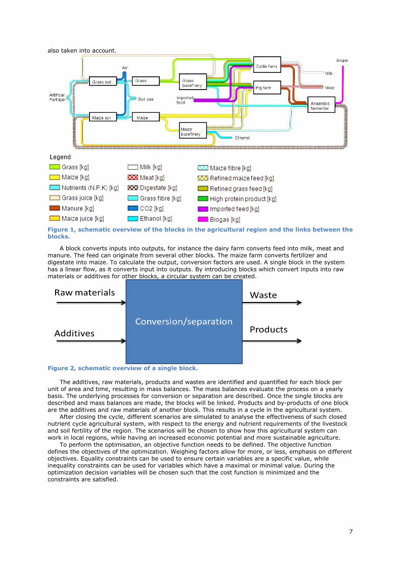
also taken into account.

Figure 1, schematic overview of the blocks in the agricultural region and the links between the blocks.

A block converts inputs into outputs, for instance the dairy farm converts feed into milk, meat and manure. The feed can originate from several other blocks. The maize farm converts fertilizer and digestate into maize. To calculate the output, conversion factors are used. A single block in the system

has a linear flow, as it converts input into outputs. By introducing blocks which convert inputs into raw materials or additives for other blocks, a circular system can be created.

Figure 2, schematic overview of a single block.

The additives, raw materials, products and wastes are identified and quantified for each block per

unit of area and time, resulting in mass balances. The mass balances evaluate the process on a yearly basis. The underlying processes for conversion or separation are described. Once the single blocks are described and mass balances are made, the blocks will be linked. Products and by-products of one block are the additives and raw materials of another block. This results in a cycle in the agricultural system.

After closing the cycle, different scenarios are simulated to analyse the effectiveness of such closed nutrient cycle agricultural system, with respect to the energy and nutrient requirements of the livestock and soil fertility of the region. The scenarios will be chosen to show how this agricultural system can work in local regions, while having an increased economic potential and more sustainable agriculture.

To perform the optimisation, an objective function needs to be defined. The objective function defines the objectives of the optimization. Weighing factors allow for more, or less, emphasis on different objectives. Equality constraints can be used to ensure certain variables are a specific value, while inequality constraints can be used for variables which have a maximal or minimal value. During the optimization decision variables will be chosen such that the cost function is minimized and the constraints are satisfied.

8

2. The agricultural system This chapter contains an overview of the theoretical background of the agricultural region. Mass

balances and underlying processes of each block are discussed. Choices and assumptions made in the model are also explained in this section.

2.1 Soil Crop cultivation is the primary production of biomass in the agricultural system. In the system two

crops are grown: grass (lolium perenne) and maize (Zea mays ssp. Mays). Both are produced to feed

livestock or to refine into various products. To cultivate any crop, a soil of sufficient quality is necessary. A fertile soil; is rich in nutrients and trace elements, has good structure to retain moisture, suitable pH and salinity, and a microbial community (Johnston et al. 2009, Powlson et al 2011, Strudley et al. 2008).

Since crop yield depends on soil quality, soil quality management is an important aspect of crop farming. As stated above, soil must contain sufficient nutrients to support plant growth. The most important nutrients are nitrogen, phosphor and potassium. Soils are often supplied with these minerals through manure and artificial fertilizers.

Artificial fertilizers usually consist of a mixture of nitrogen, phosphor and potassium, commonly referred to as NPK-Fertilizer. The nitrogen is fixed through the Haber-Bosch process, while the added

Phosphor originates from phosphate rocks. Phosphate rock is a finite resource only located in several places on earth, with most of the reserves located in Marocco and Western Sahara (USGS 2013). Recently, the depletion of the phosphate rock is heavily debated. Some scientists estimate a complete depletion of the phosphate reserves may occur in 50-100 years (Cordell et al. 2009), other scientists found no signs of short- to medium-term depletion (Vuuren et al. 2010). With the current rate of consumption, phosphate reserves would be depleted in 370 years (Scholz and wellmer 2013). However, most scientists note the increasing importance of efficient use of phosphorus and the potential to recycle and reuse phosphorus (Schröder et al. 2011, Scholz et al. 2013, van Vuuren et al. 2010).

Manure contains nitrogen, phosphate and potassium, since part of the nutrients in feed are excreted. Applying manure on agricultural land has been done throughout the history of agriculture. Application of manure increases the nutrient supply to the soil and thereby increases crop yield. However, any nutrient application on agricultural land should be managed carefully as it can result in nutrient leaching, crop

damage and soil erosion (Malhi et al. 2006, SoCo 2009). In areas of intense agriculture, eutrophication of ground water, rivers and lakes is a significant problem (Defra 2004).

Besides nutrients, soil organic matter is important as it is involved and related to many chemical, physical and biological properties (Carter, 2002). According to Diacono and Montemurro (2010), the term organic matter refers to all organic substances present in the soil. Soils also plays a vital role in the global carbon cycle; storing an estimated 109 tonnes C, twice as much as C in atmospheric CO2 (Batjes 1996). Soil organic matter has been linked to soil productivity and –quality (Lal 2002, Lal 2004, Wander and Nillsen 2004, Dumanski 2004), more precisely soil structure, moisture retention capacity, and buffering and ion exchange (Allison 1973, Waksman 1936). Organic matter decomposes in the soil, producing CO2, turns into humus, a long-lasting, amorphous, rotten dark mass. The decomposition of organic matter, by microorganisms, releases nutrients bound in the organic matter. The turnover time of

different organic materials varies considerably, from less than 3 months for crop residues up to more than 100 years for stable humus (Van-Cate et al. 2004). Sugars are decomposed quickly because they are accessible for degradation by micro-organisms. Cell walls are complex and are less accessible for degradation by the enzymes of the micro-organisms.

Since Organic matter is constantly decaying and the organic matter is important for soil quality, it needs to be added or replenished in agricultural soils. This can be done by incorporating part of the plants into the soil, spreading manure on the soil, adding soil conditioners or applying digestate. Research by Bellamy et al. (2008) has shown a decline in soil organic matter in England and Wales. This was also found by Sukkel et al. (2008) for soils in the Netherlands. Sukkel et al. (2008) observed conventional agricultural practises tend to lose more carbon compared to organic practices. However, Reijneveld et al. (2009) concluded, in a study regarding the soil organic matter in the Dutch soils between 1984 and 2004, that organic matter in soils with high organic matter concentration decreases,

while in soils with low organic matter concentration it increases. Changes in land use were found to have an effect on the soil organic matter content (Reijneveld et al. 2009).

Agricultural practices include tillage regimes. Tillage is required to prepare the soil for sowing. Different tilling regimes have different effects on the soil. Conventional tillage, characterized by annual mouldboard ploughing of the top 20-40 cm, and conservation tillage, any tillage system that reduce the loss of soil and water from cropland compared to conventional tillage (Van-Cate et al. 2004). Conventional tillage is used to control weeds and to bury plant residues and to increase organic matter in the soil (Rasmussen 1999). However, aeration of the soil results in rapid mineralization of organic matter by the microbial community and often substantial losses of nutrients, especially in warm and moist environments (Van-Cate et al. 2004). It also increases the vulnerability of the soil to erosion (Groenendijk et al. 2005, SoCo 2009). Conservational tillage decreases the vulnerability of the soil to erosion, nutrient leaching, increases soil organic matter and reduces labour and energy requirements

(Rasmussen 1999, Van-Cate et al. 2004). Tilling methods are not included in the model.

9

2.1.1 Nutrients in the soil

To model the crop cultivation, the total amount of N, P and K available for uptake from the soil is determined. C is disregarded due to the fixation of CO2 from air through photosynthesis. The potential Maize yield, in tonnes per year, on each nutrient is determined and the minimum is chosen. The nutrient associated with the lowest crop yield is considered the yield limiting nutrient. Surpluses of the other nutrients can be subtracted from their respective supply in artificial fertilizer. From the total yield, the land required for cultivation is estimated. Nutrients are supplied to the maize soil by artificial fertilizers, refinery products and digestate.

The applied nutrients are partially lost in the soil. Loss of N in the soils occurs via (1) ammonia volatilization, (2) denitrification, (3) leaching of NO3

- and (4) erosion. Ammonia volatilization can be responsible for the loss of 50% of the applied N according to McNeill and Unkovich (2007). Jarvis et al (2011) report N-efficiency from soil to crop over 75% is technically possible. Therefore, the N loss in the soil is assumed to be 25%.

Soils lose between 1 and 10 kg P/ha per year, depending on the P content of the soil (Schoumans and Groenendijk 2000). Hart et al. (2004) have found similar results, also reporting on some outliers. Hart et al. (2004) converted P loss to loss as a percentage of P applied and found most values between 1-10% with a few outliers. Therefore assuming a P loss in the soil of 10% seems reasonable.

The K efficiency in grass crops can be 90% (Pearson and Ison in: Alfaro et al. (2004)). Alfaro et al. found K leaching rates between 5 and 31 kg/ha/yr., rainfall has a big influence on K leaching. Wong et al. (1992) found that the leaching of K was below 10% in Nigerian soils. The Soil K loss in the model is

assumed to be 10%.

2.1.2 Soil organic matter model

To model the organic matter in the soil, the added organic matter and underlying process dynamics

must be described. Organic matter can be supplied to the land in various forms, i.e. plant litter, roots and microorganisms. In this model, the focus is on the lignocellulose present in the added organic matter. The digestate applied on the land has relative high lignocellulose content. More readily available substances are converted into biogas. Lignocelluloses form the additional cell wall of plant cells and consist of cellulose, hemicellulose and lignin. Lignocellulosic material is difficult to break down, thus the humification process is slower. Other cell components, such as sugar or starch, are more readily available for degradation and therefore decompose faster. With this in mind, the soil is divided into 3 compartments: A fast decomposing, slow decomposing and a biomass/humus compartment. Inputs are split between the fast decomposing and slow decomposing compartment. From these compartments, the organic matter decomposes into biomass and humus with their specific decomposition rate, releasing CO2. Biomass and humus itself is also decomposed with a specific decomposition rate. The model is

based on the organic material part of the ANIMO model (Groenendijk et al. 2005). A schematic overview is given in figure 3.

Figure 3, schematic overview of Soil organic matter model. From figure 3 mass balances over the compartments can be derived. The fast decomposing organic

matter is referred to as compartment 1, the slow decomposing organic matter is referred to as compartment 2, and the humus/biomass as compartment 3. To simplify the model, it is assumed that

10

the soil is ideally mixed, and uniform throughout the agricultural region. Soil tilling is also not included

into the model.

(

𝑑𝑀1

𝑑𝑡𝑑𝑀2

𝑑𝑡𝑑𝑀3

𝑑𝑡 )

= (

−𝑘1 0 00 −𝑘2 0

𝜀13𝑘1 𝜀23𝑘2 𝑘3

)(𝑀1𝑀2𝑀3

) + (∑ 𝑝𝑛𝐴𝑛𝑛𝑛=1

∑ (1 − 𝑝𝑛)𝐴𝑛𝑛𝑛=1

0

)

In this equation, k is the decomposition rate constant in per year, p is the fraction of input assigned

to the fast decomposing matter, A is the amount of input material in ton/hectare, M1 is the mass of the

fast decomposing organic matter pool in ton/hectare, M2 is the mass of the slow decomposing organic matter in ton/ha, M3 is the mass of the humus in ton/ha, ε is the fraction organic matter converted in to humus/biomass and n is the amount of different input materials. Analytical solutions can be found in de Willigen et al. (2008).

Lobe et al. (2002) found a lignin decomposition rate constant of 0.20 per year in soils of the South African Highveld. Wu and Mcgechen (1998) compared several dynamic soil models and found decomposition rates for fast cycling organic matter between 12 and 1 per year. Therefore, the decomposition rate constants are 2, 0.2 and 0.02 yr-1 for the fast decomposing organic matter, the slow decomposing organic matter and the biomass/humus respectively (Lobe et al. 2002, Groenendijk et al. 2005). The distribution between the slow decomposing organic matter and fast decomposing organic matter is based on previous models simulating agricultural regions, i.e. CENTURY and ANIMO (Groendendijk et al. 2005, Metherell et al. 1993).

The initial concentration of the soil organic matter is determined from literature. Groenendijk et al. (2005) use a rule of thumb; 90% of the initial soil organic matter can be attributed to humus/biomass. The top layer, 20 cm, has a weight of 2.6 million kg and has an organic matter concentration between 20 and 60 g/kg in the Netherlands (de Willigen et al. 2008). These numbers correspond to a soil organic matter concentration between 52 and 156 ton/hectare. Initial humus concentration would be between 46.8 and 140.4 ton/hectare. Other literature has found a humus reserve of 67.8 ton/hectare in Romania (Patriche et al. 2012). The 10% fresh organic matter is divided into 5% digestate and 5% fertilizer.

When organic matter is applied to the soil at a constant rate, the equilibrium concentrations can be calculated for the slow decomposing organic matter, fast decomposing organic matter and biomass/hummus by these formulas:

𝑀1,𝐸 =𝑝𝐴

𝑘1

𝑀2,𝐸 =(1 − 𝑝)𝐴

𝑘2

𝑀3,𝐸 =𝐴𝜀

𝑘3

Full analytical solutions can be found in de Willigen et al. (2008). These solutions show that the equilibrium value depends on the application rate of organic matter (A), the fraction of input assigned to the fast decomposing matter (p), the fraction converted into biomass/hummus (ε) and the decomposition rate constant (k). From these equations, the total organic matter in the soil can be calculated by summing all three equilibria. The application rate to maintain the current or acceptable organic matter concentration can also be calculated.

2.2 Maize farm Maize (Zea Mays) is an important cereal for both human nutrition and animal nutrition. In 2013 the

worldwide production of maize was 1 billion tonnes, more than rice and wheat (FAOstat, 2014). Maize is sown in spring and harvested in late summer or early autumn. Maize, especially young plants, suffer growth inhibition when temperatures are below 15 °C. Optimal growth temperatures are between 25 and 30 °C, while minimum and maximum temperature is 8 and 40°C (van Schooten et al. 2013). Apart from favourable temperatures, maize also need water, phosphate, nitrogen, carbon, potassium and

micronutrients. Most of the nutrients are taken up by the roots of the plant therefore the soil must contain sufficient nutrients. Before maize can be planted in the spring, the soil needs to be tilled. The current yield of maize per hectare, in the Netherlands, is between 11.5 and 16.5 tonnes (van Schooten et al. 2013). In Germany maize yields as high as 21.3 ton/ha has been reported, this yield was not achieved constantly however (Finke et al. 1999). In the model, maize yield is assumed to be 17 ton dry matter per hectare.

When harvested the cobs are separated from the stalk, especially when cultivated for human consumption. Stalks can be left on the land to improve soil fertility (van Schooten et al. 2013). When used for animal feed, the entire plant is sliced into small fragments and processed into silage. In silage,

11

lactic acid fermentation decreases decay thereby increasing the storage time. During the process, sugar

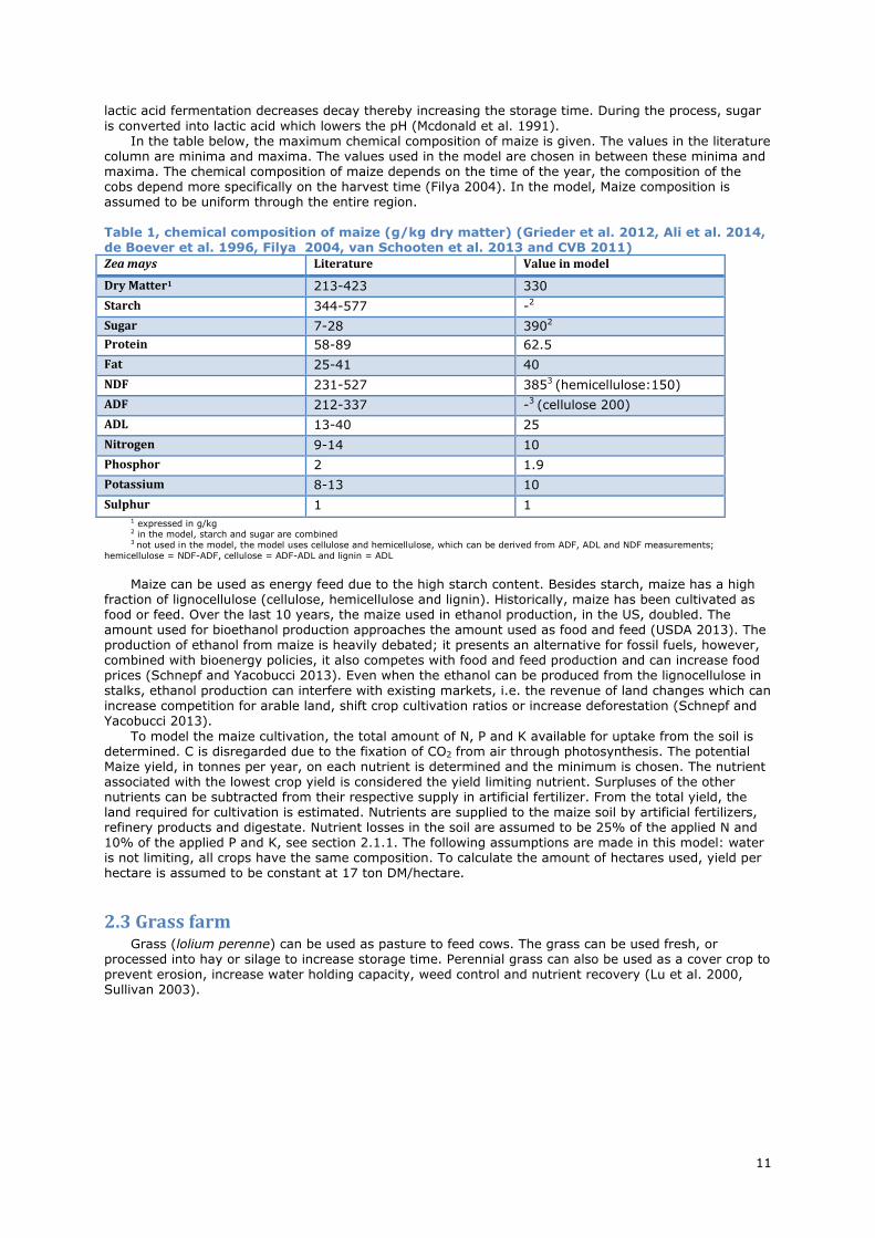
is converted into lactic acid which lowers the pH (Mcdonald et al. 1991). In the table below, the maximum chemical composition of maize is given. The values in the literature

column are minima and maxima. The values used in the model are chosen in between these minima and maxima. The chemical composition of maize depends on the time of the year, the composition of the cobs depend more specifically on the harvest time (Filya 2004). In the model, Maize composition is assumed to be uniform through the entire region.

Table 1, chemical composition of maize (g/kg dry matter) (Grieder et al. 2012, Ali et al. 2014, de Boever et al. 1996, Filya 2004, van Schooten et al. 2013 and CVB 2011)

Zea mays Literature Value in model

Dry Matter1 213-423 330

Starch 344-577 -2

Sugar 7-28 3902

Protein 58-89 62.5

Fat 25-41 40

NDF 231-527 3853 (hemicellulose:150)

ADF 212-337 -3 (cellulose 200)

ADL 13-40 25

Nitrogen 9-14 10

Phosphor 2 1.9

Potassium 8-13 10

Sulphur 1 1 1 expressed in g/kg 2 in the model, starch and sugar are combined 3 not used in the model, the model uses cellulose and hemicellulose, which can be derived from ADF, ADL and NDF measurements;

hemicellulose = NDF-ADF, cellulose = ADF-ADL and lignin = ADL Maize can be used as energy feed due to the high starch content. Besides starch, maize has a high

fraction of lignocellulose (cellulose, hemicellulose and lignin). Historically, maize has been cultivated as food or feed. Over the last 10 years, the maize used in ethanol production, in the US, doubled. The amount used for bioethanol production approaches the amount used as food and feed (USDA 2013). The production of ethanol from maize is heavily debated; it presents an alternative for fossil fuels, however, combined with bioenergy policies, it also competes with food and feed production and can increase food prices (Schnepf and Yacobucci 2013). Even when the ethanol can be produced from the lignocellulose in stalks, ethanol production can interfere with existing markets, i.e. the revenue of land changes which can increase competition for arable land, shift crop cultivation ratios or increase deforestation (Schnepf and Yacobucci 2013).

To model the maize cultivation, the total amount of N, P and K available for uptake from the soil is determined. C is disregarded due to the fixation of CO2 from air through photosynthesis. The potential Maize yield, in tonnes per year, on each nutrient is determined and the minimum is chosen. The nutrient associated with the lowest crop yield is considered the yield limiting nutrient. Surpluses of the other nutrients can be subtracted from their respective supply in artificial fertilizer. From the total yield, the land required for cultivation is estimated. Nutrients are supplied to the maize soil by artificial fertilizers, refinery products and digestate. Nutrient losses in the soil are assumed to be 25% of the applied N and 10% of the applied P and K, see section 2.1.1. The following assumptions are made in this model: water is not limiting, all crops have the same composition. To calculate the amount of hectares used, yield per hectare is assumed to be constant at 17 ton DM/hectare.

2.3 Grass farm Grass (lolium perenne) can be used as pasture to feed cows. The grass can be used fresh, or

processed into hay or silage to increase storage time. Perennial grass can also be used as a cover crop to prevent erosion, increase water holding capacity, weed control and nutrient recovery (Lu et al. 2000, Sullivan 2003).

12

Table 2, chemical composition of grass (g/kg dry matter) (Jancik et al. 2010, Cone and van

Gelder 1999, Klop et al. 2008, Smit et al. 2006, Sauvant et al. 2002 and CVB 2011)

Lolium perenne Literature Value in model

Dry Matter1 115-280 -3

Starch 0 -2,3

Sugar 80-100 1802

Protein 175-239 200

Fat 31-44 40

NDF 431-600 5003 (hemicellulose:225)

ADF 215-344 -3 (cellulose: 250)

ADL 16-43 25

Nitrogen 28-38 33

Phosphor 2-4 4

Potassium 16-37 25

Sulphur 1-3 3 1 expressed in g/kg 2 in the model, starch and sugar are combined 3 not used in the model, the model uses cellulose and hemicellulose, which can be derived from ADF, ADL and NDF measurements;

hemicellulose = NDF-ADF, cellulose = ADF-ADL and lignin = ADL Table 2 shows the high protein content of ryegrass, making it ideal as a protein supply in feed. Grass

cultivation complements the maize cultivation in the system. Maize is considered an energy crop due to the high sugar and starch content while grass is rich in protein. This combination gives the agricultural system an efficient supply in both energy and protein. The dry matter yield of ryegrass per hectare is between 10 and 15 (Wilkins 1989, Daepp et al. 2000, Pinxterhuis et al. 2013)

Grass is often grown in combination with clovers to make use of the biological nitrogen fixing capabilities of clovers (Dahlin and Stenberg 2010). Grass is dominant in dry weight yields in such systems, accounting for 80-90% of the yield. The dry weight yield of clover is estimated between 20-

10%. Carlsson and Huss-Danell (2003) found a relation between the dry weight yield percentage of white clover (Trifolium Repens L.) and the biological nitrogen fixation per hectare:

𝐵𝑁𝐹 = 0.031 ∗ 𝐷𝑀 + 24 In this formula, BNF is the biological nitrogen fixation in kg N per hectare and DM is the yield of

white clover in kg per hectare. When white clover accounts for 10% of the dry matter yield, the dry matter yield is 1 t/ha, resulting in a BNF of 55 kg N/ha. A dry matter yield of 2 t/ha results in a BNF of 86 kg N/ha.

The model calculates total amount of nutrients supplied to the crop and then determines the total yield. From the total yield, the area of the land can be calculated. To prevent an endless loop of increasing land leading to increased BNF which results in more land; the total amount of biological nitrogen fixation is estimated at 500 ton N per year. This number is estimated using previous results regarding the area of grass land in the system, as this number is always in the same order of magnitude.

The grass cultivation model assumes the clover have a similar composition as the ryegrass.

2.4 Crop rotation The intensification in agriculture resulted in minimal or inefficient crop rotation. Studies have shown

the effects of monocultures include soil degradation, need for artificial fertilizers and weed control, nutrient leaching, loss of biodiversity and increase in fossil fuel use (Karlen et al. 1994, Giller et al. 1997 Tilman et al. 2002, Malezieus et al. 2009, Bullock 1992). An alternative for monocultures is crop rotation, growing different crops in different years on other parts of the farm. Crop rotation enhances soil fertility, soil structure and organic matter, combats soil erosion and the use of artificial fertilizers, diversifies the

products and spreads the work of a farmer through the year (Zegada-Lizarazu and Monti 2011). However, disadvantages of crop rotation include higher levels of farm organisation, additional equipment for new crops, reduced land for the crops with the highest economic profit and require farmers to stick with the planned rotation thus losing the option to choose contingently (Zegada-Lizarazu and Monti 2011). Farmers need to overcome unfamiliarity with potential new crops used in the rotation.

Kalmlage et al. (2010) concluded that using a 1-year maize followed by 2-year grass rotation offers potential to reduce the risk of elevated N leaching and groundwater pollution while achieving satisfying yields. Pinxterhuis et al. (2013) also note the potential to use maize-grass systems, however they also include triticale. The preferred arable land use ratio between grass and maize in a 2-year grass 1-year maize system is; 2 ha grass: 1 ha maize. This ensures a constant production of both grass and maize.

13

2.5 Small scale biorefinery Biorefinery, defined according to IEA Bioenergy (2009), is the sustainable processing of biomass into

a spectrum of marketable products and energy. This definition includes the many aspects and facets of biorefinery. The sustainable processing of biomass is an attractive prospect to shift from a fossil fuel economy, towards a bio-based economy. The bio-based economy relies on the renewable production of biomass. The shift towards a bio-based economy has several drivers; an over dependency on phosphorus and fossil fuel imports, the finite nature of both resources and the limited countries exporting phosphorus and fossil fuels, but also climate change and development of rural areas are important drivers towards a bio-based economy (Langeveld et al. 2010, OECD 2009). Closing cycles is often part of the bio-based economy; this would reduce the import of nutrients.

Due to the many applications of biorefinery, Cherubini et al (2009) proposed a classification method based on (1) platform, (2) products, (3) feedstock and (4) processes. Platforms, the intermediates which link the products and feedstock, are central in Cherubini et al.’s approach as different processes can

convert different materials into these platforms. Other processes can be used to convert the platforms into different products. The platforms are: biogas, syngas (a mix of CO and H2), hydrogen, C6 sugars, C5 sugars, lignin, pyrolysis liquid, oil, organic juice and electricity. Products are classified into two main categories, energy and materials (including chemicals, feed, food and fertilizer). The feedstock used in biorefinery is the renewable raw material and come from four sectors: Agriculture, Aquaculture, Forestry or Industry. Further distinction can be made between dedicated feedstocks, grown for the purpose of biorefinery, or residues. The processes can be categorized into four groups: mechanical/physical, biochemical, chemical and thermochemical processes. (Cherubini et al. 2009)

In this study, two small scale biorefineries are introduced in an agricultural system. Bruins and Sanders (2012) note several advantages of small scale biorefineries: (1) Reduction of transportation. (2) Increasing the possibility for immediate recycling of water and other fractions separated during the process. (3) Processing locally can improve storage time and help reduce the seasonal dependency on

some agricultural products. (4) Employment in rural areas increases and (5) the investment and innovation costs are lower. Bruins and Sanders (2012) also note that large scale processes offer advantages with regards to the lower production cost per product, more efficient heat transfer and generally large scale processes can achieve higher conversions. According to Bruins and Sanders (2012), a cleverly designed process split in two parts, can make use of all advantages.

This agricultural system includes both large scale and small scale processing. The small scale biorefineries are a grass biorefinery and maize biorefinery. The grass biorefinery separates grass into several fractions before further distribution. During the process the fibres are separated from the protein, which enables non-ruminants to feed on the proteins cultivated in grass. The maize biorefinery ferments starch in maize to produce ethanol. A third biorefinery process is also introduced: a biogas fermenter. The biogas fermenter aims to retrieve as much energy as possible from manure and left over biomass. All three biorefineries introduced in the system have been tested at pilot scale therefore the proposed

system could be implemented in the near future without need for extensive development for the biorefineries.

2.5.1 Grass biorefinery

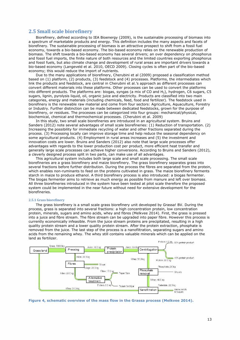
The grass biorefinery is a small scale grass biorefinery unit developed by Grassa! BV. During the process, grass is separated into several fractions: a high concentration protein, low concentration protein, minerals, sugars and amino acids, whey and fibres (Melkvee 2014). First, the grass is pressed into a juice and fibre stream. The fibre stream can be upgraded into paper fibre. However this process is currently economically infeasible. From the juice stream proteins are precipitated, resulting in a high quality protein stream and a lower quality protein stream. After the protein extraction, phosphate is removed from the juice. The last step of the process is a nanofiltration, separating sugars and amino acids from the remaining whey. The whey still contains valuable minerals which can be applied on the land as fertilizer.

Figure 4, schematic overview of the mass flow in the Grassa process (Melkvee 2014).

14

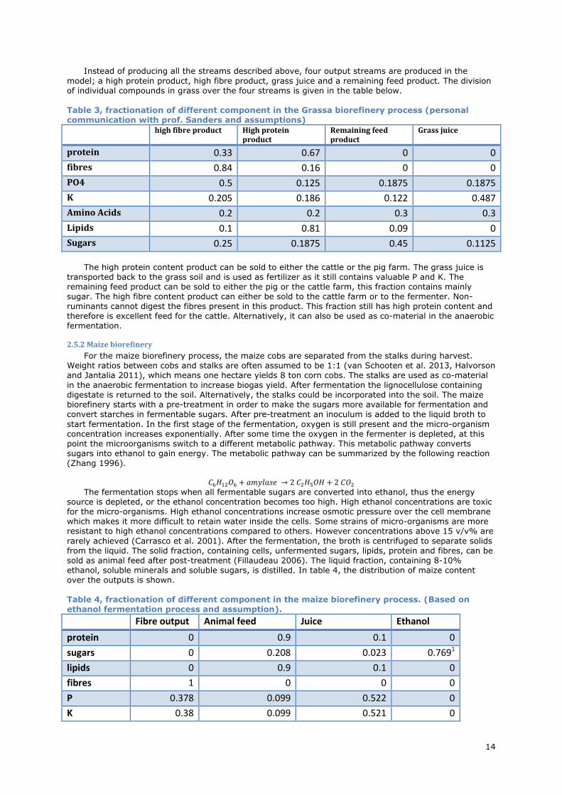
Instead of producing all the streams described above, four output streams are produced in the

model; a high protein product, high fibre product, grass juice and a remaining feed product. The division of individual compounds in grass over the four streams is given in the table below.

Table 3, fractionation of different component in the Grassa biorefinery process (personal communication with prof. Sanders and assumptions)

high fibre product High protein product

Remaining feed product

Grass juice

protein 0.33 0.67 0 0

fibres 0.84 0.16 0 0

PO4 0.5 0.125 0.1875 0.1875

K 0.205 0.186 0.122 0.487

Amino Acids 0.2 0.2 0.3 0.3

Lipids 0.1 0.81 0.09 0

Sugars 0.25 0.1875 0.45 0.1125

The high protein content product can be sold to either the cattle or the pig farm. The grass juice is transported back to the grass soil and is used as fertilizer as it still contains valuable P and K. The remaining feed product can be sold to either the pig or the cattle farm, this fraction contains mainly sugar. The high fibre content product can either be sold to the cattle farm or to the fermenter. Non-ruminants cannot digest the fibres present in this product. This fraction still has high protein content and therefore is excellent feed for the cattle. Alternatively, it can also be used as co-material in the anaerobic fermentation.

2.5.2 Maize biorefinery

For the maize biorefinery process, the maize cobs are separated from the stalks during harvest. Weight ratios between cobs and stalks are often assumed to be 1:1 (van Schooten et al. 2013, Halvorson and Jantalia 2011), which means one hectare yields 8 ton corn cobs. The stalks are used as co-material in the anaerobic fermentation to increase biogas yield. After fermentation the lignocellulose containing digestate is returned to the soil. Alternatively, the stalks could be incorporated into the soil. The maize biorefinery starts with a pre-treatment in order to make the sugars more available for fermentation and convert starches in fermentable sugars. After pre-treatment an inoculum is added to the liquid broth to

start fermentation. In the first stage of the fermentation, oxygen is still present and the micro-organism concentration increases exponentially. After some time the oxygen in the fermenter is depleted, at this point the microorganisms switch to a different metabolic pathway. This metabolic pathway converts sugars into ethanol to gain energy. The metabolic pathway can be summarized by the following reaction (Zhang 1996).

𝐶6𝐻12𝑂6 + 𝑎𝑚𝑦𝑙𝑎𝑠𝑒 → 2 𝐶2𝐻5𝑂𝐻 + 2 𝐶𝑂2

The fermentation stops when all fermentable sugars are converted into ethanol, thus the energy source is depleted, or the ethanol concentration becomes too high. High ethanol concentrations are toxic for the micro-organisms. High ethanol concentrations increase osmotic pressure over the cell membrane which makes it more difficult to retain water inside the cells. Some strains of micro-organisms are more resistant to high ethanol concentrations compared to others. However concentrations above 15 v/v% are

rarely achieved (Carrasco et al. 2001). After the fermentation, the broth is centrifuged to separate solids from the liquid. The solid fraction, containing cells, unfermented sugars, lipids, protein and fibres, can be sold as animal feed after post-treatment (Fillaudeau 2006). The liquid fraction, containing 8-10% ethanol, soluble minerals and soluble sugars, is distilled. In table 4, the distribution of maize content over the outputs is shown.

Table 4, fractionation of different component in the maize biorefinery process. (Based on ethanol fermentation process and assumption).

Fibre output Animal feed Juice Ethanol

protein 0 0.9 0.1 0

sugars 0 0.208 0.023 0.7691

lipids 0 0.9 0.1 0

fibres 1 0 0 0

P 0.378 0.099 0.522 0

K 0.38 0.099 0.521 0

15

1 This is sugar, which is converted into ethanol during the fermentation according to the reaction described above.

Distilling results in a 60% V/V ethanol product and a residue. The residue contains minerals and

some soluble sugars. The 60% ethanol is sold while the residue can be returned to the soil. The animal feed produced during the byosense process has a better digestibility compared to the unprocessed input,

due to the thermal pre-treatment (Kiers et al. 2000). From the reaction equation given above, the remaining sugar can be calculated, as well as the maximum theoretical ethanol yield.

2.6 Livestock

2.6.1 Dairy farm

Since cattle has been domesticated in early human history (Sauvant et al. 2002), they were held to produce meat, dairy products and hides. Through breeding, cattle is often specialized in either meat or milk production (Theunissen, 2012). However cattle held for dairy production purposes still produce meat. Today, dairy farming has become a science where nutritional and energy demands, milk production, animal welfare, feed quality, genetics and sheltering are researched (Larkin 2011, Drackley et al. 2006, Raussi 2003,). Dairy farmers also face the challenge to reduce their environmental impact, especially related to manure and emission of methane and ammonia, and increase the animal welfare,

while maintaining the production. Energy, protein and water are considered to be the most important aspects of the dairy cows’ diet

(Eastridge 2006, Cabrita et al. 2007). Annually, a single dairy cow requires 42.3 GJ energy and 554 kg of digestible protein, exact calculation are described in appendix I calculation of energy and protein requirement for a cow (Remmelink et al. 2013). Beside energy and protein, dairy cows nutritional requirements include various minerals and vitamins (Drackley et al. 2006). In the agricultural system 5 different feeds are included; maize, grass, refined maize, refined grass and imported feed. The imported feed is assumed to have a composition similar to soybean meal.

The manure is collected and further processed in the anaerobic fermenter. The composition of the manure has an impact on the ability to recycle nutrients throughout the agricultural system. Dairy cows are ruminants, meaning their stomach consists of multiple compartments with microorganisms able to degrade recalcitrant fibres like cellulose and hemicellulose. In table 4 the manure characteristics are

presented. In Appendix III the digestibility of different lignocellulosic materials are estimated. The digestibility of cellulose, hemicellulose and lignin are estimated at 60%, 80% and 5% respectively. The manure of dairy cattle still contains considerable amounts of lignocellulose. The digestibility of lignocellulose in dairy cattle is assumed to be constant. The composition of the manure is determined by mass balances over the cattle. Parts of the lignocellulose are broken down, while the N, P and K are allocated to manure, meat or milk. For N 66% of the input is allocated to manure (Kohn et al. 2005, Nadeau et al. 2007). It is assumed 66% of the P fed to the dairy cattle ends up in the manure (Borucki et al. 2004). The recommended P intake for dairy cattle is 27 kg per year (Sehested 2004). Manure receives 67% of the K in the feed (Bannink et al. 1999). The N allocated to milk is 32% of the input. For P this is 28% and for K 33% of the input nutrients in the feed (Arriaga et al. 2008, Bannink et al. 1999). The remaining parts are allocated to the meat. The amount of nutrients held up in the meat is relative

small, since the meat production is small compared to the manure and milk production. The water and feed requirement per kg of product is given in table 3. Producing beef seems

inefficient as the required feed and water is about 10 times higher compared to the production of milk. However, due to the prices producing beef is economically feasible. The price for beef is about 10 times as high as the price for milk (LEI, 2013).

Table 5, inputs and outputs of dairy cows related to amount of product (kg/ kg product).

Inputs Outputs Source

Product Water Feed Manure

Beef 55 8 38 Fleming 2001, Sebek 2009, ASAE 2005, Ward 2007

Milk 4 0.8 2 Fleming 2001, ASAE 2005, Ward 2007, Mekonnen 2010

According to Remmelink et al. (2013) cows start lactating when they are two years old. Dairy cows are marketed as beef once they reach an age of 5.7 (CVR 2013). Average weight for an adult dairy cow is 650 kg. When slaughtered 300 kg of meat is produced, the rest is used for non-dietary purposes. The modelled agricultural region consists of 20000 dairy producing cows. The entire cow population is turned over after 3.6 productive years, resulting in annual marketing of 5556 dairy cows. For dairy cows to maintain milk production, calves have to be born. Female calves are used to replace older dairy cows. A few male calves are either used as breeding bull and the rest is marketed as beef or veal.

2.6.2 Pig farm

Domestication of pigs occurred about 9.000 years ago (Bökönyi 1974, Epstein and Bichard 1984). Pigs are mainly held for meat production. After World War II, intensive pig husbandry replaced mixed farming, increasing the pig meat production (Geels 2009). The mass production of pig meat decreased

16

the production costs however intensive pig farming has also been criticized frequently (Fraser 2005).

Current research within pig farming focuses on the environmental impact, health concerns, animal welfare, nutrition and productivity (Veillette et al. 2012).

Energy, protein and water are considered the most important aspects of the diet. Often, pig feed is enriched with antibiotics to prevent diseases inside the pig farm (Tilman et al. 2002). Since pigs are omnivores, and thus able to handle a versatile diet, pigs are more efficient meat producers compared to cattle. In table 6, the relation between inputs and outputs, and product is given. Compared to the inputs required per kg product, pigs require much less feed and water. Furthermore, pigs produce lower quantities manure compared to dairy cattle. Dairy cows consume more dray matter in a day compared to pigs

Table 6, inputs and outputs of pigs related to the amount of product (kg/kg product).

Inputs Output Source

Product water feed Manure

Pork 7 4.2 7.5 Fleming 2001, Sebek 2009, ASAE 2005, Ward 2007, Mekonnen 2010

The pig farm in our model contains 100000 pigs, used for meat production. Pigs, like dairy cows,

require water, energy and nutrients. Energy and protein are commonly regarded as most important aspects of the pig’s diet. In appendix II, the total energy requirements for the pigs are calculated. In the model, equality constraints are introduced to make sure pigs receive sufficient protein and energy. The equality constraint is set at 6000 tonnes protein per year and the energy constraint is set at 500000 GJ per year.

Beside meat, the pig farm produces manure. In table 7 the characteristics of pig manure are given. Similar to dairy cattle manure, pig manure contains lignocellulose and nutrients like N, P and K. However, the pigs’ ability to digest cellulose, hemicellulose and lignin is lower compared to ruminants. In appendix III the digestibility of these materials is determined at 30%, 60% for cellulose and hemicellulose respectively. Lignin is not digested in the intestines of pigs. In the model the digestibility of

lignocellulose is assumed to be constant as long as the lignocellulose content of the feed is within acceptable boundaries.

The N, P and K excretion are determined by using conversion factors from the amount fed to the pig. It is assumed that 70% of the ingested N is excreted in the manure (Kohn et al. 2005), 66% of the P is excreted in the manure (van Krimpen et al. 2010, Bikker et al. 2013) and 70% of the K is excreted. Pigs have a higher nutrient hold up compared to cattle because pigs grow significantly more in the system. This is also reflected in the lifespan of both animals, the average time dairy cattle is in the system is 3.6 years, while the average pig time is about 200 days. Reducing the nutrient excretion in this model can be done by either assuming higher uptake efficiencies or reducing the nutrients in the diet. Reduction of nutrients in the diet can result in deficiency of the nutrients and compromises animal welfare. It is assumed that any possible micro-nutrient deficiency can be solved by diet supplements.

2.7 Anaerobic fermentation Manure excess is a growing problem in many countries including the Netherlands (CBS 2014). A

method to valorise the excess manure is by anaerobic digestion. During anaerobic digestion, manure is fermented to CH4 which can be captured and utilised as biogas. Anaerobic digestion offers significant benefits over other waste treatment methods. Compared to aerobic digestion, less sludge is produced (Ward et al. 2008). Other benefits include the capability to treat wastes with low total solid content (Peck and Hawkes 1987), good pathogen removal (Lund et al. 1996, Sahlström 2003), the slurry can be used as soil conditioner and fertilizer (Tamboneet al. 2009, Vaneeckhaute et al. 2013a, Alburquerque et al.

2012) and the biogas production. Different designs of anaerobic digesters are used in practice. These can be categorized in three main

groups: batch reactors, continuously fed single reactor systems and continuously fed multiple reactor systems (Ward et al. 2008). The Batch reactor system is the simplest: feedstock is loaded into the reactor and left for a period of time for reactions to take place. In continuously fed single reactor systems, all reactions occur in a single tank. The continuously fed multiple tank systems divide different reactions between different tanks. This allows separate optimization of the hydrolysis, acidification, acetogenesis and methanogenesis. Often, hydrolysis and acidification are separated from acetogenesis and methanogenesis, as these processes do not share the same optimal conditions (Ward et al. 2008).

Using only manure as feedstock resulted in disappointing biogas production (Callaghan et al. 1999), due to high ammonia concentrations inhibiting the methanogenesis (Van Velzen 1979). Co-digestion

offers an option to create more favourable C: N ratios in the reactor by adding a biomass feedstock (Ward et al. 2008, Alatriste-Mondragón et al. 2006) thereby increasing biogas production (Callaghan et al. 1999). Other advantages of co-digesting include the ability to process two wastes simultaneously and the digestion of poorly degradable wastes (Alatriste-Mondragón et al. 2006). Ammonia can also be removed by using an acidic air scrubber, resulting in an N and S rich stream which can be used as synthetic fertilizer substitute (Vaneeckhaute et al. 2013b).

17

2.7.1 The anaerobic fermenter model

The amount of methane produced in the biogas fermenter can be estimated from a steady state mass balance. The mass balance is made with chemical oxygen demand per year as unit. Chemical

oxygen demand (COD) is the mass of oxygen required to completely oxidize a compound to carbon dioxide, water and ammonia.

𝐶𝑛𝐻𝑎𝑂𝑏𝑁𝑐 + (𝑛 +𝑎

4−𝑏

2−3

4𝑐)𝑂2 → 𝑛 𝐶𝑂2 + (

𝑎

2−3

2𝑐)𝐻2𝑂 + 𝑐 𝑁𝐻3

From the equation above, the amount of moles required to fully oxidize a general compound, CnHaObNc. The COD can be expressed in g O2/g substrate or in g O2/mole substrate.

The COD mass balance over the biogas fermenter consists of an influent, an effluent, COD converted to microorganisms and COD converted to methane.

0 = 𝐼𝑛𝑓𝑙𝑢𝑒𝑛𝑡 𝐶𝑂𝐷 − 𝐸𝑓𝑓𝑙𝑢𝑒𝑛𝑡 𝐶𝑂𝐷 − 𝐶𝑂𝐷 𝑡𝑜 𝑚𝑖𝑐𝑟𝑜𝑜𝑟𝑔𝑎𝑛𝑖𝑠𝑚𝑠 − 𝐶𝑂𝐷 𝑡𝑜 𝑚𝑒𝑡ℎ𝑎𝑛𝑒 To determine the amount of COD to methane, the amount of COD in the influent, effluent and to

microorganisms should be determined. The COD in the influent and effluent depend on the composition of both streams. The effluent consists of undigested material. The influent consists of manure from

livestock and lignocellulose from the biorefineries in our system. To determine the COD of the lignocellulose material the molecular formula should be known. Since cellulose is a polysaccharide, the molecule formula of a single monomer, (C6H10O5)n, can be used. Cellulose has a COD of 1185 g O2 per kg cellulose. Hemicellulose also consists of multiple sugars thus the COD of hemicellulose is the same. The molecular formula for lignin is more complicated as it has aromatic structures and differs through time and between species. In this study, the molecule formula for lignin is assumed to be C31H34O11 (Zakzeski et al. 2010). Using this molecular formula results in a COD for lignin of 1900 g O2 per kg lignin.

When the incoming mass of lignocellulose is known, the COD of the influent can be calculated. The COD in the effluent can be determined by using digestion factors. The digestion of cellulose, hemicellulose and lignin are assumed to be 0.5, 0.7 and 0.25, respectively. From the influent COD and the digestion factors, the effluent COD can be calculated.

To determine the amount of COD converted to biomass, the amount of biomass needs to be

calculated first. According to Metcalf and Eddy (2004), the biomass production can be calculated with the following formula:

𝑃𝑥 =𝑌 ∗ 𝑄 ∗ (𝑆0 − 𝑆)

1 + 𝑘𝑑𝑆𝑅𝑇

In which Px is the biomass production in kg/day, Y the yield coefficient of microorganisms in g biomass/ g COD, Q*(S0-S) the amount of COD consumed in the reactor per day, kd, the death rate of the microorganisms in day-1 and SRT, the time the solids remain in the digester, in days.

Metcalf and Eddy (2004) report Y values between 0.05 and 0.10 while kd is between 0.02 and 0.04 for the entire anaerobic digestion process. Q*(S0-S) is the amount of COD consumed per day in the biogas fermenter and can be determined from the total influent and effluent COD. The SRT is a design parameter which is generally between 20 and 30 days. The amount of microorganisms produced per year

needs to be converted to COD in the microorganisms. Assuming the microorganisms have a composition close to the general composition, the molecular formula C5H7O2N can be used (Hoover and Porges 1952). From this general microorganism composition the COD of the microorganisms can be determined; 1 kg of microorganisms is equal to 1.42 kg COD (Metcalf & Eddy 2004).

With the COD contributed by microorganisms known, the COD for methane can be calculated by subtracting the effluent and microorganism COD from the influent COD. The methane COD can be converted to a volume, at 35° C 1 kg COD is equal to 0.4 m3 CH4. It can also be converted to a mass, 1

mole of methane has a COD of 64 grams O2 while the molar mass of methane is 16 gram. With the microorganism mass known, the nutrient holdup in the microorganisms can be determined.

Magidan et al. (1997) described the dry weight elemental composition of microorganisms; this is presented in table below. The amount of nutrients stored in the microorganisms is important for the nutrient supply to the soil.

Table 7, typical composition of bacteria cells (weight fractions) (Magidan et al. 1997).

element fraction

Carbon 0.5

Oxygen 0.22

Nitrogen 0.12

Hydrogen 0.09

Phosphorus 0.02

Sulphur 0.01

Potassium 0.01

18

Other elements 0.03 The microbial biomass can be separated, along with undigested solids, by centrifugation. The solids

are applied to the agricultural land as soil conditioner. A variable is introduced to determine which fraction going to the maize soil and which is going to the grass soil. The microbes in the solids are considered fast digesting material in the soil model. The digestion speed of the remaining solids depends on the origin, i.e. lignin, protein, cellulose and hemicellulose.

2.7.2 Estimating H2S concentration in the biogas

During the anaerobic fermentation, sulphur in the feed can be converted into H2S. H2S has a foul

odour and upon combustion can be converted into highly corrosive, unhealthy and environmental unfriendly SO2 (Abatzoglue and Boivin 2009). Peu et al. (2012) noted that hydrogen sulphide concentrations must be lower than 100-500 mg/m3 to prevent equipment damage. To predict hydrogen sulphide production in the biogas fermenter a mass balance is used.

0 = 𝑆 𝑖𝑛 − 𝑆 𝑜𝑢𝑡 − 𝑆 𝑡𝑜 𝑚𝑖𝑐𝑟𝑜𝑜𝑟𝑔𝑎𝑛𝑖𝑠𝑚𝑠 − 𝑆 𝑖𝑛 𝑔𝑎𝑠 First, the amount of S in the inputs is determined from literature. Cattle manure, pig manure, grass

and maize have a total S content of 2, 4, 3 and 1 g/kg dry matter, respectively (van Schooten et al. 2013, Peu et al. 2012). The input of dry matter is calculated in the optimization thus the input of S into the biogas fermenter can be calculated. Next is the S in the microorganisms, from the biomass production, calculated above, and the elemental composition of biomass, the amount of S in the microorganisms can be determined. The method to determine the H2S concentration in the gas is based on carbon degradation. Peu et al. (2012) found a relation between the fraction of sulphur available for

reduction and the biodegradability of carbon. Peu et al. (2012) further concluded that once sulphur is reduced, the phase transfer is non-limiting. Peu et al. (2012) found that the molar ratio in the input of the feed in the anaerobic fermenter is a decent predictor for the H2S concentration in the biogas. The biogas therefore has the same molar ratio between S and C as the feed, thus assuming sulphur has the same degradability as carbon. The percentage of H2S in the biogas is calculated using the following formula

𝑉𝑜𝑙𝑢𝑚𝑒 % 𝐻2𝑆 =𝑆/32

𝐶/12∗ 100%

S is the sulphur influent and C the carbon influent, this is converted into mol. The molar mass of sulphur is 32 g/mole and the molar mass of carbon is 12 g/mol.

2.7.3 Digestate

After fermentation, the digestate is separated into a solid and liquid fraction. Different solid-liquid separation techniques can be used, i.e. centrifugation or filtration. The digestate contains undigested lignocellulose and other material, dissolved nutrients and micro-organisms. Separation of the digestate is more beneficial to comply with legal standards. For the distribution of nutrients over the two fractions the following assumptions have been made: All micro-organisms are allocated to the solid fraction, as is all the remaining lignocellulosic material. 66% of the N is in the liquid phase, half of the P is distributed to the liquid fraction and 90% of the K is allocated to the liquid fraction (Fuchs and Drosg 2013). The liquid and solid fractions of the digestate are separately distributed over the maize and grass land.

2.10 Dutch fertilizer law To combat pollution, the Dutch fertilizer law limits the application of nutrients on agricultural soil.

The law focuses on two nutrients; nitrogen and phosphorus. Nitrogen application on land can result in the formation of NOx compounds and the leaching of NO3

- and NO2- to ground water. Phosphorus

leaching can result in the eutrophication of various water bodies. The maximum application of nitrogen and phosphorus depends on the crop selection, ground type,

and period of cultivation and for phosphorus also the phosphorus content of the soil. More details can be found in appendix IV. The Dutch fertilizer law aims to reduce the supply of these nutrients to the amount of nutrients removed upon harvest. Maize has a maximal nitrogen application of 140 kg N/ha. For low

phosphorus soils the maximum is 75 kg P2O5/ha. For grass the maximal nitrogen application is 320 kg N/ha and 100 kg P2O5/ha on low P soils.

The P fertilization rate is calculated by adding all the P supplied to the grass soil and dividing it by the total area of the grass soil, the same is done for the maize soil. This total can be converted to P2O5 equivalents by dividing the mass by 0.436, the fraction of P in P2O5. Calculating the N application involves weighing factors, as not type of N fertilizer counts equal to the maximum. In this report the following assumptions are made with regards to N fertilizers and the law:

The application of artificial N fertilizer counts 100% towards the legal maximum. The cattle manure and pig manure are digested in the same installations and separated in a liquid and solid fraction after digestion. Thus there are three different weighing factors towards the law: 100% for artificial fertilizer, 80% for the liquid fraction of the digestate and 55% for the solid fraction of the digestate. More details on the fertilizer law can be found in appendix IV.

19

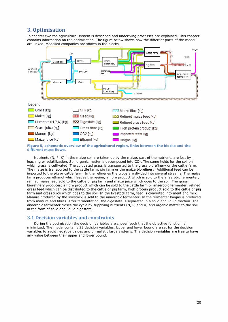
20

3. Optimisation In chapter two the agricultural system is described and underlying processes are explained. This chapter contains information on the optimisation. The figure below shows how the different parts of the model are linked. Modelled companies are shown in the blocks.

Figure 5, schematic overview of the agricultural region, links between the blocks and the different mass flows.

Nutrients (N, P, K) in the maize soil are taken up by the maize, part of the nutrients are lost by leaching or volatilization. Soil organic matter is decomposed into CO2. The same holds for the soil on which grass is cultivated. The cultivated grass is transported to the grass biorefinery or the cattle farm. The maize is transported to the cattle farm, pig farm or the maize biorefinery. Additional feed can be imported to the pig or cattle farm. In the refineries the crops are divided into several streams. The maize farm produces ethanol which leaves the region, a fibre product which is sold to the anaerobic fermenter,

refined maize feed sold to the cattle or pig farm and maize juice which goes to the soil. The grass biorefinery produces; a fibre product which can be sold to the cattle farm or anaerobic fermenter, refined grass feed which can be distributed to the cattle or pig farm, high protein product sold to the cattle or pig farm and grass juice which goes to the soil. In the livestock farm, feed is converted into meat and milk. Manure produced by the livestock is sold to the anaerobic fermenter. In the fermenter biogas is produced from manure and fibres. After fermentation, the digestate is separated in a solid and liquid fraction. The anaerobic fermenter closes the cycle by supplying nutrients (N, P, and K) and organic matter to the soil in the form of solid and liquid digestate.

3.1 Decision variables and constraints During the optimisation the decision variables are chosen such that the objective function is

minimized. The model contains 23 decision variables. Upper and lower bound are set for the decision variables to avoid negative values and unrealistic large systems. The decision variables are free to have any value between their upper and lower bound.

21

Table 8, list of decision variables in the agricultural system, their units and the upper and

lower bounds.

# Name decision variable unit Lower bound Upper bound

1 Imported feed for cattle Ton 0 41000

2 Imported feed for pigs Ton 0 31000

3 Artificial nitrogen fertilizer for grass Ton N 0 2000

4 Artificial phosphorus fertilizer for grass Ton P 0 2000

5 Artificial potassium fertilizer for grass Ton K 0 2000

6 Artificial nitrogen fertilizer for maize Ton N 0 3000

7 Artificial phosphorus fertilizer for maize Ton P 0 2000

8 Artificial potassium fertilizer for maize Ton K 0 2000

9 Maize for maize refinery Ton 0 100000

10 Maize for cattle consumption Ton 0 200000

11 Maize for pig consumption Ton 0 100000

12 Grass for grass refinery Ton 0 100000

13 Grass for cattle consumption Ton 0 200000

14 Fraction of refined maize for cattle - 0 1

15 Fraction of grass for refinery - 0 1

16 Fraction maize to refinery - 0 1

17 Fraction maize to cattle - 0 1

18 Fraction maize to pigs - 0 1

19 Fraction protein product from grass refinery to cattle - 0 1

20 Fraction refined grass feed to cattle - 0 1

21 Fraction of solids from fermenter to grass soil - 0 1

22 Fraction of liquid from fermenter to grass soil - 0 1

23 Fraction of fibre product from grass refinery to cattle - 0 1

The system has to be opened somewhere to start the optimisation. It is chosen to break the links

between the crop farms and the biorefineries/livestock farms. Closing the system at this point requires the fewest constraints. Five links are broken, the links between; grass farm and the grass refinery, grass farm and the cattle farm, maize farm and the maize refinery, maize farm and the cattle farm and between the maize farm and the pig farm. Equality constraints are used to replace these broken links. The grass leaving the grass farm to the refinery must be equal to the grass which is refined, (X_grassb=Y_grassb). This should also be satisfied for the other broken links (X_grassc=Y_grassc,

X_maisb=Y_maisb, X_maisc=Y_maisc and X_maisp=Y_maisp). These constraints ensure the model remains a cycle. The distribution factors, decision variable 15 to 18, are used to calculate the Y_grassb, Y_grassc, Y_maisb, Y_maisc and Y_maisp. The other fractions are used to determine the mass distribution for products with multiple destinations.

Energy and protein constraints for livestock are required to satisfy the demands of the livestock. This ensures the production of animal produce in the region. The energy supply to the cattle must be equal to 8.7*105 GJ/year and for pigs 5.0*105 GJ/year. Protein constraints are set at 22000 ton/year for cattle and 6000 ton/year for pigs. Another constraint is added to prevent the sum of fractions of the maize distribution becoming larger than 1. This results in a total of 10 equality constraints.

3.2 Objective function The goal of the optimisation has to be defined in the objective function. The goals need to be

expressed in mathematically, because the optimisation minimizes the objective function. The objective function can contain multiple goals. When multiple goals are present in the objective function, weighing factors can be used to put more, or less, emphasis on certain goals. Generally an objective functions with two goals looks like this:

𝑓 = 𝑤1𝑦1 +𝑤2𝑦2 This objective function tries to minimize y1 and y2. The weighing factor, w, represents the importance

of a goal. Only the ratio between the weighing factors matters, therefore one of the weighing factors can be chosen as 1. The objective function can also contain states of the system (x) and inputs of the system (u).

In this study, the objective function contains two goals; maximizing total profit and minimizing the

area of land use within the agricultural region. The total profit is maximised because the agricultural region needs to make a healthy profit. Larger total profit means bigger incomes for the people in the region and result in higher welfare in the region. Previous results show the system can increase when optimising on total profit alone, therefore the land use is minimised in the objective function.

A weighing factor is associated with each goal. The objective function is expressed in euro; therefore the weighing factor of the total profit is fixed at 1. This weighing factor is dimensionless because the total profit is expressed in euro. The weighing factor on land use is in euro per ha. The objective function of the optimisation looks like this:

𝑓 = −(𝑡𝑜𝑡𝑎𝑙 𝑝𝑟𝑜𝑓𝑖𝑡) + 𝑤1 ∗ (𝑙𝑎𝑛𝑑 𝑢𝑠𝑒)

22

The weighing factor, also called the land use penalty, is a cost for using land in the system. A series

of optimisations is performed with an increasing penalty on land use to study how the land use penalty affects the agricultural region.

Several optimisations are performed with different weighing factors. The weighing factors used during the optimisation are 0, 1, 100, 1000, 2000, 4000, 5000, 6000, 8000 and 10000. When the weighing factor is 0, the land use penalty is not taken into account. Thus the model is solely optimised on total profit. The other weighing factors are chosen to study the system behaviour. Even though total profit and land use are the main objectives of this optimisation, other properties of the agricultural region can also be interesting. This objective function is used to study the behaviour of the region when the area of land use is changed.

3.3 Initial guesses Initial guesses for the decision variables must be supplied to give the optimisation a starting point.

The optimisation routine then changes the decision variables to minimize the objective function and satisfy the constraints, upper and lower bounds. The optimisation routine cannot distinguish a local minimum for the objective function from the global minimum. Therefore, the initial guess can have an influence on the outcome. To minimize this influence, the initial guess for all decision variables is changed randomly at the start of an optimisation. The time to calculate a single outcome is very short. The optimisation routine calculates for 15 minutes and returns the lowest objective function value found during the 15 minutes. In 15 minutes, many different initial guesses are calculated. This reduces the influence of the initial guess. The values of the decision variables associated with the lowest objective function value can be used as new initial guesses.

23

24

4. Results This chapter contains the results of various optimisations including some comments and additional

explanations on some results.

4.1 Land use series In this series of optimisations the following objective function has been used:

𝑓 = −(𝑡𝑜𝑡𝑎𝑙 𝑝𝑟𝑜𝑓𝑖𝑡) + 𝑤1 ∗ (𝑙𝑎𝑛𝑑 𝑢𝑠𝑒) There are two parts of this component; the total profit of the system and the land use with a

weighing factor. To create the series, the weighing factor is increased to punish the land use more severe. The factors used are: 0, 1, 100, 1000, 2000, 4000, 5000, 6000 and 10000. The weighing factor can be seen as a land use penalty and has a unit of €/ha. Note that land use only covers the arable land used within the region used for grass and maize cultivation. The series consists of 18 optimisations are performed. In the figures, the numbers 1 to 18 represent the outcome of the optimisation. In the table below the weighing factor for each optimisation can be found.

Table 9, optimisation number and corresponding land use penalty. # 1 2 3 4 5 6 7 8 9 10 11 12 13 14 15 16 17 18

Land use penalty (euro/ha)

0 1 102 103 103 103 2*

103

2*

103

4*

103

4*

103

5*

103

5*

103

6*

103

6*

103

8*

103

8*

103

104 104

4.1.1 Total profit and land use

Figure 6, objective function, total profit and area of land use plotted against the weighing factor. (With area of land on the secondary y-axis)

In figure 6, objective function, total profit and area of land use are plotted. This figure shows how

the main goals of the optimisation behave with different weighing factors. Logically, no land use penalty results in the highest profit agricultural system, although a land use penalty of 1000 or 2000 euro/ha does not affect the total profit much. The area of land use and total profit decrease when the weighing factor increases.

The height of the penalty determines how much the system focuses on area of land use reduction. Therefore the land use penalty can be used to steer the system. Land use penalties can be used as a policy instrument in agricultural regions, thus figure 6 shows the model can be valuable in analysing such policies.

25

Figure 7, individual total profit (left) and area of land use (right) plotted against the land use penalty.

The figure above shows that a land use penalty of 5000 euro per hectare already reduces the area of

the agricultural region from 17500 ha to 9200 ha. The total profit in the region is reduced by 26%. When the land use penalty is larger than 6000 euro per hectare, the optimisation constantly results in an agricultural region of about 9200 ha.

When a land use penalty is introduced, the area of land use decreases more than the total profit, therefore the profit per hectare increases. The profit per hectare is shown in Figure 8.

Figure 8, total profit per hectare plotted against the land use penalty (left) and area of land use (right).

When land use is punished severely, the model prefers to produce most of the most profitable products (milk). However the number of cows is set and thus the milk production cannot increase beyond a certain value, therefore the model starts to produce less profitable products and thus profit per area

starts to decrease. Maximizing profit per hectare would result in trying to minimize the area of land used by the system because area of land can be reduced without decreasing profit through import. Therefore it is chosen not to optimise on profit per hectare.

4.1.2 Import in the agricultural region

In figure 6, at a land use penalty of 5000 there are clearly 2 points for the objective function value, optimisation 11 and 12. The lower value, optimisation 11, is optimised better towards the main goals, total profit and area of land use. But the agricultural system is a regional system, thus optimisation 12 may have advantages over optimisation 11 which are not included in the objective function. In the following section other properties of the agricultural region will be discussed.

Figure 9, total profit and total import plotted against land use penalty and area of land use. (With total profit on the secondary y-axis)

In figure 9 the import into the system and the total profit in the system is plotted against the land

use penalty on the left and area of land use on the right. Import in the system consists of the sum of the feed import and artificial fertilizer import. There are clearly two types of system; optimisation 1-8 which are low import systems with high area of land use within the region and optimisation 10, 11 and 13-18

26

which are high import system with low area of land use. Optimisation 9 and 12 are in between these two

extremes. When the import is high, the self-sufficiency of the system is low.

Figure 10, imported feed and fertilizer plotted against the penalty on land use. (With imported fertilizer on the secondary y-axis)

The penalty on land use results in a lower area of land in the agricultural region; this reduces the

production of feed within the region. This decrease has to be compensated by a higher import of animal

feed. At the same time, a lower area of land use requires fewer artificial fertilizer imports. This shows how punishing land use within the system can affect other aspects of the region.

High import-low land use systems and low import-high land use systems. The points in purple are a

compromise between these two, making them interesting systems. The high import systems manage to have a herd of 20000 cows and 100000 pigs on 9000 ha land. 9000 hectare is roughly 10 % of the agricultural area of the Achterhoek. When the region increases in size, the import decreases because feed imports are replaced by artificial fertilizer imports. Furthermore, an increase in land use results in a higher total profit. Lower land use systems do have a higher profit per hectare, meaning the profit of additional land use decreases.

4.1.3 Phosphorus excretion

From the obtained data, the P excretion in manure can also be plotted against the area of land use. Since the amount of proteins fed to the livestock is set as an equality constraint and the N in manure is calculated by using a conversion factor, the N excretion for all systems should be equal.

Figure 11, P excretion plotted against area of land use.

27

The total P excretion in the systems decreases when the area of land use increases. The P excretion

for both livestock decreases different. For cows, initially the P excretion decreases. At around 13000 ha the P excretion becomes more or less constant. For pigs, the initial P excretion remains constant, after around 13000 ha the P excretion in pigs starts to decline. The P excretion is related to the diet composition of the animals. A higher P content in the feed results in a higher P content in the manure.

Figure 12, diet composition of pigs (left) and cattle (right) plotted against area of land use.

(Optimisations 13 to 18 are all around 9200 ha) For pigs, the diet in low land use systems consists mainly of imported feed and maize. When the

area of land use increases over 13000 ha, the imported pig feed in the diet starts to decline, while the refined products increase. This change matches the change in P excretion and can be explained by the lower P content of the refined feed over the imported feed. This shows the environmental benefit of having refineries in the system. For cattle the diet changes initially; imported feed is replaced by grass cultivated in the system. The mass of refined feed remains relative constant. This shows an environmental benefit of producing grass locally with respect to P excretion. The imported feed for the cattle is replaced first since the profit margin on cattle products is larger. When the imported feed for cattle becomes marginal the imported pig feed starts to decrease.

From the two animal diet figures it can be concluded that small land use systems require large

imports of feed to maintain livestock numbers. The land required for the cultivation of imported feed is not included in the area of land use. This presents an interesting problem in self-sufficiency; for the currently available land (9000 ha) the number of animals can only be achieved with a large quantity of imported feed.

Note that P excretion is analysed in an optimal situation for land use and total profit. The P excretion, or other goals, can be added in the objective function. In this study the objective function is not increased beyond 2 goals, because the weighing of the objectives with 3 or more goals becomes very subjective.

4.1.4 Biorefineries

Some of the outcomes found during the optimisation completely disregard the biorefineries; this can be seen in figure 13. In optimisation 10, 11, 13, 14, 15 and 16 the biorefineries hardly make profit, the mass which is refined is also be small.

Figure 13, biorefinery profit plotted against land use penalty.

28

Figure 14, profit (left) and mass input (right) of the individual biorefineries.

Note that as the penalty on land use increases, the land use decreases as does the mass which is

refined. The mass of maize which is refined drops quickly. The mass grass used for refinery decreases slightly. Both refineries generate more economic profit when the input increases. The profit the grass refinery makes is higher than the maize refinery even though the maize refinery sometimes refines much more mass.

Interestingly, the optimisation for a land use penalty of 10000 euro/ha finds a biorefinery annual profit of more than 2 million. While some outcomes between land use penalties of 4000 and 8000 find very low profits for biorefineries. Low profits indicate low usage of biorefineries. It is possible that the systems found with a 10000 euro/ha land use penalty are local minima. This could depend on the initial guess of the optimisation, if it is set close to a strong local minima, it may not find a better minima on the other side of the spectrum. Nonetheless, these systems can be interesting when taking more goals into account than the land use and total profit. From the model it follows that the N removed from the system is also replenished. Furthermore, protein supply to the livestock is set as an equality constraint therefore the N in the system is fixed.

4.1.5 Soil organic matter

The digestate from the fermenter is returned to the grass soil and maize soil. Below is a graph showing the long term effect of this digestate. Note that any other method to supply organic matter is not taken into account. For instance, contribution of the root systems of the harvested crops is not taken into account. The initial soil organic matter content is estimated at 52 ton per hectare. Since the crop rotation in the system is 2 years of grass cultivation followed by a year of maize cultivation, the digestate

application rate is calculated by averaging the application rate over the 3 years. Thus the digestate application rate of grass counts twice and the maize rate once.

Figure 15, equilibrium soil organic matter in a 2:1 grass: maize rotation.

For systems with low land use, the soil organic matter is between 26 and 30 ton/ha. Slightly larger

systems have lower soil organic matter, while the large systems have higher soil organic matter.

Compared to the initial condition, the soil organic matter difference is small. On average the soils lose 23 ton soil organic matter per hectare. The moment when the steady state is reached depends on the organic matter type. The fast decomposing organic matter will reach a new equilibrium in 3 years, the

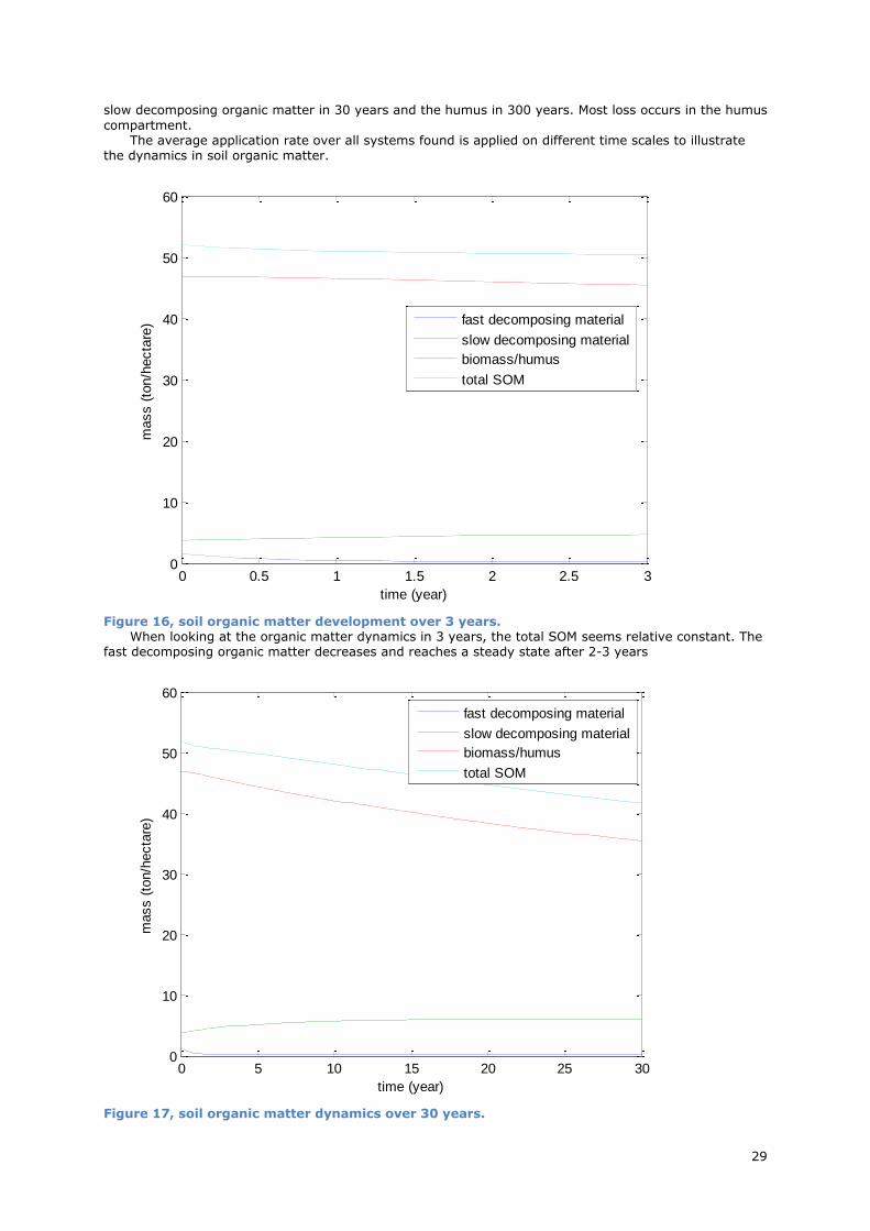
29

slow decomposing organic matter in 30 years and the humus in 300 years. Most loss occurs in the humus

compartment. The average application rate over all systems found is applied on different time scales to illustrate

the dynamics in soil organic matter.

Figure 16, soil organic matter development over 3 years.

When looking at the organic matter dynamics in 3 years, the total SOM seems relative constant. The fast decomposing organic matter decreases and reaches a steady state after 2-3 years

Figure 17, soil organic matter dynamics over 30 years.

0 0.5 1 1.5 2 2.5 30

10

20

30

40

50

60

time (year)

mass (

ton/h

ecta

re)

fast decomposing material

slow decomposing material

biomass/humus

total SOM

0 5 10 15 20 25 300

10

20

30

40

50

60

time (year)

mass (

ton/h

ecta

re)

fast decomposing material

slow decomposing material

biomass/humus

total SOM

30

The total SOM decreases significant over 30 years, this is mainly casued by change in the biomass/humus content. The slow decomposing organic matter content increases. It reaches a steady state after roughly 20 years.

Figure 18, soil organic matter dynamics over 300 years.

Over 300 years, the total SOM also reaches the new steady state, just below 30 ton/ha. The most significant contributor is the humus. Slow decomposing material increases, while the fast decomposing matter is insignificant over the course of 300 years.

In short term, less than 10 years, the soil organic matter should be fine. Even with only the application of the digestate. However over longer periods of time, soil organic matter could become problematic. This behaviour is caused by the different time constants (1/k) of the system. The most important time-constant for the total soil organic matter is the time constant of the humus, since humus

contributes most to the total.

4.1.6 Crop rotation in the agricultural region

In the theoretical background crop rotations are introduced. The preferred crop rotation is 2 years of

grass cultivation followed by 1 year maize cultivation. To check if this rotation can be performed, the land distribution between grass and maize is plotted.

0 50 100 150 200 250 3000

10

20

30

40

50

60

time (year)

mass (

ton/h

ecta

re)

fast decomposing material

slow decomposing material

biomass/humus

total SOM

31

Figure 19, percentage of grass and maize land in the agricultural region.

In every system in the series, the land used for grass cultivation is higher than the land used for

maize cultivation. Some systems have a good land use ratio, optimisation 4, 5, 6, 8, 9 and 12. Other systems are close to a 60:40 grass maize ratio. The ideal ratio is 2:1 grass-maize land. When regions deviate from this ratio, there is a slight annual difference in crop yields. Thus one year there is a bit more maize, while the next 2 years there is a bit less. None of the systems deviate far from the 2:1

ratio.

4.2 P excretion series In the land use series, it was concluded that smaller agricultural systems have a higher P excretion.

Higher P excretion results in more stress on the environment. Modern agricultural regions should take the excretion of nutrients into account. The Dutch fertilizer law already limits the application of nutrients on soil, which has resulted in an excess of nutrients in manure. Therefore, reducing the amount of nutrients in the manure reduces the excess of manure and helps reduce environmental stress. To achieve this, a series of optimisations is performed with total profit and P excretion in the objective

function. The land use series showed that the agricultural region tends to increase in size when it is not limited, therefore the system can use a maximum of 15000 ha. This is added as an inequality constraint. The system needs some flexibility in order to reduce the P excretion; therefore the system is limited at 15000 ha. This results in the following objective function:

𝑓 = −(𝑡𝑜𝑡𝑎𝑙 𝑝𝑟𝑜𝑓𝑖𝑡) + 𝑤1 ∗ (𝑃𝑒𝑥𝑐𝑟𝐶𝑜𝑤 + 𝑃𝑒𝑥𝑐𝑟𝑃𝑖𝑔)

The decision variables and constraints given in chapter 3 still apply. There is one additional constraint in the form of: 𝑎𝑟𝑒𝑎 𝑔𝑟𝑎𝑠𝑠 + 𝑎𝑟𝑒𝑎 𝑚𝑎𝑖𝑧𝑒 ≤ 15000 ℎ𝑎. The total number of decision variables is still

23, the number of equality constraints is 10, and there is an inequality constraint. Upper and lower

bounds are unchanged. The weighing factor in the objective function, also called the penalty on P excretion, is expressed in euro per ton P excreted.

The manure also contains excess N, causing environmental stress. N is not included in the objective function because the protein intake of the livestock is used as an equality constraint. Therefore the N supply to the livestock is fixed. In the system a constant is used to convert feed into manure and produce. Therefore, the excreted N in the model is constant and cannot be optimised in this model.

In the series, 12 different weighing factors for the P excretion are used. The different optimisations

are numbers 1 to 12 and the corresponding penalty on P excretion can be found in the table below. Table 10 , optimisation numbers and corresponding P excretion penalty.

# 1 2 3 4 5 6 7 8 9 10 11 12

P excr. penalty (euro/ton P)

0 0 2000 2000 4000 4000 6000 6000 8000 8000 10000 10000

4.2.1 Total profit and P excretion

First the objective function value is plotted together with the total profit and the P excretion. The total profit is plotted as negative total profit to prevent a huge difference on the y-axis (negative total profit = - (total profit)).

32

Figure 20, objective function value, total profit and total P excretion of the P excretion series. (With total P excretion on the secondary y-axis)

The objective function value increases as the weighing factor on P excretion increases. At the same

time, the total P excretion decreases. The total profit seems to be relative constant as the weighing factor on P increases. From figure 20 it can be concluded that the main aim of the optimisation is achieved; the system can become less polluting by introducing a penalty on P excretion and the pollution

is reduced without a change in total profit.

Figure 21, total P excretion (left) and total profit (right) of the P excretion series.

When a P excretion penalty of 8000 is used, the P excretion drops from 360 ton P to 335 ton P, a 7%

decrease in excretion. Increasing the penalty beyond 8000 euro per ton P seems to have little effect on the P excretion. Optimisation 7 is interesting; it has a low P excretion and the highest profit of all

optimisations. When looking at the y-axis of the total profit, the difference in total profit seems to be small, this means that reduced P excretion can be achieved at low costs.

There is a linear relation between P intake and P excretion in the model, the P intake must have been reduced. It is interesting to see the origin of the diets of the cattle and pigs.

Figure 22, P excretion (left) and diet composition of cattle in the P excretion series.

From the figure above with the cattle diet and P excretion, it can be concluded that there is no change in the diet of the cattle. Therefore the cattle excrete the same amount of P in all optimisations.

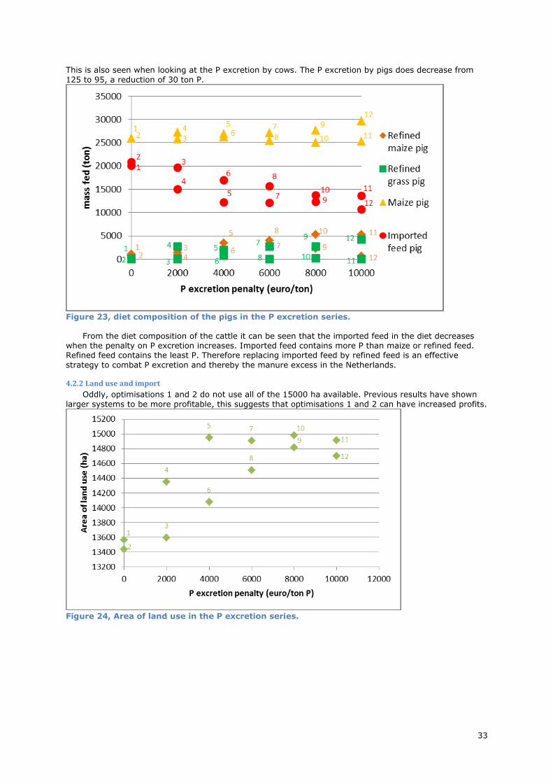
33

This is also seen when looking at the P excretion by cows. The P excretion by pigs does decrease from

125 to 95, a reduction of 30 ton P.

Figure 23, diet composition of the pigs in the P excretion series.

From the diet composition of the cattle it can be seen that the imported feed in the diet decreases

when the penalty on P excretion increases. Imported feed contains more P than maize or refined feed. Refined feed contains the least P. Therefore replacing imported feed by refined feed is an effective

strategy to combat P excretion and thereby the manure excess in the Netherlands.

4.2.2 Land use and import

Oddly, optimisations 1 and 2 do not use all of the 15000 ha available. Previous results have shown

larger systems to be more profitable, this suggests that optimisations 1 and 2 can have increased profits.

Figure 24, Area of land use in the P excretion series.

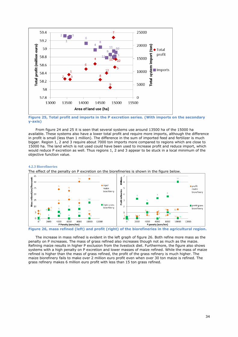
34

Figure 25, Total profit and imports in the P excretion series. (With imports on the secondary y-axis)

From figure 24 and 25 it is seen that several systems use around 13500 ha of the 15000 ha available. These systems also have a lower total profit and require more imports, although the difference in profit is small (less than 1 million). The difference in the sum of imported feed and fertilizer is much bigger. Region 1, 2 and 3 require about 7000 ton imports more compared to regions which are close to

15000 ha. The land which is not used could have been used to increase profit and reduce import, which would reduce P excretion as well. Thus regions 1, 2 and 3 appear to be stuck in a local minimum of the objective function value.

4.2.3 Biorefineries

The effect of the penalty on P excretion on the biorefineries is shown in the figure below.

Figure 26, mass refined (left) and profit (right) of the biorefineries in the agricultural region.

The increase in mass refined is evident in the left graph of figure 26. Both refine more mass as the

penalty on P increases. The mass of grass refined also increases though not as much as the maize. Refining maize results in higher P exclusion from the livestock diet. Furthermore, the figure also shows systems with a high penalty on P excretion and lower masses of maize refined. While the mass of maize refined is higher than the mass of grass refined, the profit of the grass refinery is much higher. The maize biorefinery fails to make over 2 million euro profit even when over 30 ton maize is refined. The grass refinery makes 6 million euro profit with less than 15 ton grass refined.

35

4.2.4 Soil organic matter

The effect on soil organic matter can be plotted in a similar to the land use series; the average of two times the application rate of organic matter on grass soil and once the application rate on maize.

Figure 27, equilibrium soil organic matter in the agricultural region.

When equilibrium is reached, half of the soil organic matter initially present is lost. The loss patterns

are similar to figures 16, 17 and 18. Thus the loss of soil organic matter is a concern in long term. However the added organic matter from the root-systems is not taken into account in these simulations.

4.3 Individual systems From the previous results, it was shown that there are trends in the series. In this section several

agricultural regions are presented in more detail. Some of these systems are also in the previous results,

others are obtained with different objective functions. The land use series and P excretion series showed that the design of the agricultural region can differ. Seven agricultural regions are chosen to be discussed in more detail and to show how the regions vary;

Region 1: one of the large systems from the land use series, more specifically optimisation 1 of the land use series. This system is characterised by optimising on total profit only, it is the region with the largest area of land use within the Netherlands. Furthermore it has low imports and a high total profit.

Region 2: region 18 from the land use series. This system has a very low area of land use, 9300 ha. Imports are required to satisfy the protein and energy demands of the livestock.

Region 3: from the P excretion series region 7 is included. This region had the highest total profit and still managed to have a low P excretion.

Region 4: in the P excretion series, the area of land use is capped at 15000 ha. This much area may

not be available. Therefore, one of the regions chosen is a region which is optimised on total profit and P-excretion with a maximum area of land use of 12000 ha.

Region 5: one of the outcomes of the optimisation for region 5 refined surprisingly little biomass, but achieved a low objective function value. Therefore this system is included as one of the regions.

Region 6: this region replaces soybean-based animal feed import with a refined rapeseed product. The objective function used in this optimisation only contains economic profit. The maximum area of land use was set at 12000 ha. A maximum of 12000 ha was chosen to ensure the system requires feed imports. Unlimited systems tend to increase the area of land use within the system. The maximum of 12000 ha still allows for some flexibility. The composition of the refined rapeseed product can be found in appendix V.

Region 7: this region was the outcome of a simulation with an objective function with total profit and P excretion in it. The area of land use is limited to maximally 12000 ha. The weighing factor used for the

P excretion was 1000 euro/ton P. This system is not included in the P excretion series because it clearly is a local outcome. I included this agricultural region on a personal note, because the outcome shows how several important factors in the region could be balanced. These factors include area of land use, import in the region, P excretion and total profit of the region. It must be stressed that this region is not a good solution with respect to its objective function value. However, in my opinion it makes a solid agricultural region.

In all the optimisations performed the decision variables and equality constraints are unchanged. Upper and lower bounds are also unchanged. (See: Chapter 3. Optimisation)

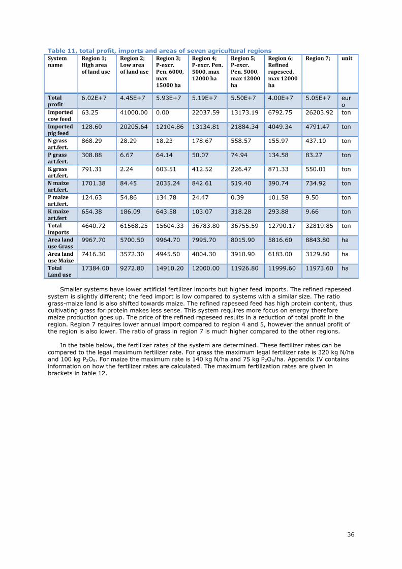
36

Table 11, total profit, imports and areas of seven agricultural regions

System name

Region 1; High area of land use

Region 2; Low area of land use

Region 3; P-excr. Pen. 6000, max 15000 ha

Region 4; P-excr. Pen. 5000, max 12000 ha

Region 5; P-excr. Pen. 5000, max 12000 ha

Region 6; Refined rapeseed, max 12000 ha

Region 7;

unit

Total profit

6.02E+7 4.45E+7 5.93E+7 5.19E+7 5.50E+7 4.00E+7 5.05E+7 euro

Imported cow feed

63.25 41000.00 0.00 22037.59 13173.19 6792.75 26203.92 ton

Imported pig feed

128.60 20205.64 12104.86 13134.81 21884.34 4049.34 4791.47 ton

N grass art.fert.

868.29 28.29 18.23 178.67 558.57 155.97 437.10 ton

P grass art.fert.

308.88 6.67 64.14 50.07 74.94 134.58 83.27 ton

K grass art.fert.

791.31 2.24 603.51 412.52 226.47 871.33 550.01 ton

N maize art.fert.

1701.38 84.45 2035.24 842.61 519.40 390.74 734.92 ton

P maize art.fert.

124.63 54.86 134.78 24.47 0.39 101.58 9.50 ton

K maize art.fert

654.38 186.09 643.58 103.07 318.28 293.88 9.66 ton

Total imports

4640.72 61568.25 15604.33 36783.80 36755.59 12790.17 32819.85 ton

Area land use Grass

9967.70 5700.50 9964.70 7995.70 8015.90 5816.60 8843.80 ha

Area land use Maize

7416.30 3572.30 4945.50 4004.30 3910.90 6183.00 3129.80 ha

Total Land use

17384.00 9272.80 14910.20 12000.00 11926.80 11999.60 11973.60 ha

Smaller systems have lower artificial fertilizer imports but higher feed imports. The refined rapeseed

system is slightly different; the feed import is low compared to systems with a similar size. The ratio grass-maize land is also shifted towards maize. The refined rapeseed feed has high protein content, thus cultivating grass for protein makes less sense. This system requires more focus on energy therefore maize production goes up. The price of the refined rapeseed results in a reduction of total profit in the region. Region 7 requires lower annual import compared to region 4 and 5, however the annual profit of the region is also lower. The ratio of grass in region 7 is much higher compared to the other regions.

In the table below, the fertilizer rates of the system are determined. These fertilizer rates can be

compared to the legal maximum fertilizer rate. For grass the maximum legal fertilizer rate is 320 kg N/ha and 100 kg P2O5. For maize the maximum rate is 140 kg N/ha and 75 kg P2O5/ha. Appendix IV contains information on how the fertilizer rates are calculated. The maximum fertilization rates are given in brackets in table 12.

37

Table 12, fertilization rates and manure excess.

(Maximum legal fertilization rate is given between brackets)

System name

Region 1; High area of land use

Region 2; Low area of land use

Region 3; P-excr. Pen. 6000, max 15000 ha

Region 4; P-excr. Pen. 5000, max 12000 ha

Region 5; P-excr. Pen. 5000, max 12000 ha

Region 6; Refined rapeseed, max 12000 ha

Region 7;

unit

Grass N fert rate

318.60 (320)

237.83 (320)

335.00 (320)

285.89 (320)

264.36 (320)

266.51 (320)

279.96 (320)

kg N/ha

Grass P2O5 fert rate

89.36 (100)

93.86 (100)

89.31 (100)

89.36 (100)

89.39 (100)

90.56 (100)

89.20 (100)

kg P2O5/ha

Maize N fert rate

179.12 (140)

131.67 (140)

126.65 (140)

152.23 (140)

200.49 (140)

140.31 (140)

189.80 (140)

kg N/ha

Maize P2O5 fert rate

87.81 (75)

82.95 (75)

82.65 (75)

82.31 (75)

82.31 (75)

82.31 (75)

82.31 (75)

kg P2O5/ha

System P capacity

677.10 365.36 596.18 453.29 477.38 455.79 487.93 Ton P

P placed 784.05 474.83 553.40 479.55 458.98 482.79 453.07 Ton P

System N capacity

3752.70 2032.42 3331.91 2679.66 2668.83 2505.26 2743.02 ton N

N placed 2995.20 2995.20 2995.20 2995.20 2995.20 2995.20 2995.20 ton N

The system P and N capacity is the total amount of P and N which can be placed on the arable land.

When more P or N is placed in the system there is a manure excess. Only one system has sufficient

capacity to place all nutrients in the system, which is region 3. This is the system which has a penalty on P excretion of 6000 euro per ton P and a maximum of 15000 ha. All systems are over the maximum amount of nutrients from animal excreta because digestate counts fully towards the maximum placement of animal excreta. Region 7 is close to placing all the nutrients in the system. Regions close to the placing capacity reduce the manure excess significantly.

Table 13, profit per block. System name

Region 1; High area of land use

Region 2; Low area of land use

Region 3; P-excr. Pen. 6000, max 15000 ha

Region 4; P-excr. Pen. 5000, max 12000 ha

Region 5; P-excr. Pen. 5000, max 12000 ha

Region 6; Refined rapeseed, max 12000 ha

Region 7;

unit

Maize refinery profit

2.72E+6 5.69E+4 7.20E+5 4.21E+5 8.38E+2 1.11E+2 4.29E+4 €

Grass refinery profit

3.51E+6 2.96E+6 3.36E+6 4.44E+6 4.47E+2 1.57E+03 9.85E+6 €

Cattle farm profit

2.02E+7 1.17E+7 2.04E+7 1.53E+7 1.87E+7 7.33E+06 1.35E+7 €

Pig farm profit

-2.38E+6 2.63E+6 -1.56E+5 -2.24E+5 3.64E+6 -8.34E+5 -4.65E+6 €

Anaerobic digester profit

-4.10E+6 2.59E+6 3.90E+5 2.10E+6 3.20E+6 3.42E+6 2.81E+6 €

Grass farm profit

2.11E+7 1.37E+7 2.06E+7 1.86E+7 1.89E+7 1.32E+7 2.11E+7 €

Maize farm profit

1.91E+7 1.09E+7 1.39E+7 1.12E+7 1.06E+7 1.69E+7 7.78E+6 €

38

Figure 28, profit of the blocks in the region

In table 13 and the figure above it can be seen that the crop farms always make profit. Through

photosynthesis, Crops convert light into chemical energy. Therefore, the energy supply to the crops is free which increases the profit margins substantially. The profit of the refineries differs greatly between the systems. The biorefineries in the system with the refined rapeseed have a low annual profit. This can

be explained by the high protein content of the refined rapeseed; more focus is on maize cultivation for the energy in maize. The maize biorefinery extracts energy from the maize and the grass refinery focuses on proteins which are already supplied by the rapeseed. The cattle farm generates a healthy profit; most of the turnover is generated by milk. The pig farm makes a profit when it imports a lot of feed. The biorefinery increases the price of feed which reduces the profit margin. The separated fibres increase costs of the anaerobic fermenter resulting in decreased profit. Region 7 generates a lot of profit through the grass biorefinery. The large area of grass in the system can be explained; Region 7 produces a lot of protein in the system, this is refined and fed to the pigs. The refined product is more expensive, thus lowers the pig farms profit.

Table 14, P excretion

System name Region 1; High area of land use

Region 2; Low area of land use

Region 3; P-excr. Pen. 6000, max 15000 ha

Region 4; P-excr. Pen. 5000, max 12000 ha

Region 5; P-excr. Pen. 5000, max 12000 ha

Region 6; Refined rapeseed, max 12000 ha

Region 7;

unit

P excretion pig

45.85 121.90 92.97 96.40 126.43 51.32 68.38 ton P

P excretion cattle

241.10 285.99 241.24 266.99 257.20 195. 277.02 ton P

Total P in manure

286.95 407.88 334.21 363.39 383.63 246.63 345.41 ton P

The P excretion by livestock is reduced by the refined rapeseed. The P content in the refined

rapeseed is much lower compared to the soybean import. However, in this system there is more P placed

on the agricultural land than legally allowed. This can be caused by the change of land use towards maize. Maize land has a lower maximum for P fertilization, thus having more maize land reduces the placing capacity of P, this also holds for N. Region 7 reduces the P excretion significantly compared to region 4 and 5. This reduces stress on the environment as the manure contains less P.

39

Table 15, distribution of refined produce.

System name Region 1; High area of land use

Region 2; Low area of land use

Region 3; P-excr. Pen. 6000, max 15000 ha

Region 4; P-excr. Pen. 5000, max 12000 ha

Region 5; P-excr. Pen. 5000, max 12000 ha

Region 6; Refined rapeseed, max 12000 ha

Region 7;

unit

refined grass product to pig

2750.46 1032.35 2732.54 2777.84 0.35 0.25 6141.37 ton

refined grass product to cow

0.51 4886.36 34.13 5920.71 0.02 2.88 12753.40

ton

refined maize products to pig

10314.82

0.00 2729.08 990.55 2.98 0.19 2.19 ton

refined maize products to cow

476.22 214.48 0.00 604.50 0.15 0.04 159.50 ton

fraction refined grass protein to cow

0.04 0.64 0.01 0.07 0.01 0.75 0.01 -

fraction refined grass feed to cow

0.05 0.36 0.01 0.81 0.15 1.00 1.00 -

fraction refined grass fibre to cow

0.08 1.00 0.00 0.97 0.01 1.00 0.93 -

In the table above it can be seen that some systems refine high quantities of crops while some other

systems hardly refine crops. When a significant mass of grass is refined, most of the products seem to be assigned for pig consumption, although there are some systems which send the feed fraction to the cattle. The fraction of fibres transported to the cattle is high in systems which have a low area of land use.

Table 16, Biological nitrogen fixation and yield limiting nutrient for grass.

System name Region 1; High area of land use

Region 2; Low area of land use

Region 3; P-excr. Pen. 6000, max 15000 ha

Region 4; P-excr. Pen. 5000, max 12000 ha

Region 5; P-excr. Pen. 5000, max 12000 ha

Region 6; Refined rapeseed, max 12000 ha

Region 7;

unit

BNF 50.16 87.71 50.18 62.53 62.38 85.96 56.54 kg N/ha

Clover fraction on grass

0.08 0.21 0.08 0.12 0.12 0.20 0.10 -

Limiting nutrient grass

N N N N K N N

When looking at the biological nitrogen fixation, most of the clover fractions are between 0.08 and

0.12. These fractions of clover in the grassland are in line with expectations. Two systems have around

20% clover in the grass. These systems also have much lower grass land compared to the other systems. One system is a system with only 9000 ha, while the other is the refined rapeseed system. In only one system, grass cultivation is not limited by N. Table 17, equilibrium of soil organic matter

System name Region 1; High area of land use

Region 2; Low area of land use

Region 3; P-excr. Pen. 6000, max 15000 ha

Region 4; P-excr. Pen. 5000, max 12000 ha

Region 5; P-excr. Pen. 5000, max 12000 ha

Region 6; Refined rapeseed, max 12000 ha

Region 7;

unit

Application rate lignocellulose

2.03 1.70 1.69 1.66 1.54 1.60 1.50 ton/ha

Equilibrium fast organic matter

0.30 0.25 0.25 0.25 0.23 0.24 0.22 ton SOM /ha

Equilibrium slow organic matter

7.13 5.95 5.91 5.84 5.40 5.60 5.25 ton SOM /ha

Equilibrium humus

25.63 21.37 21.24 20.97 19.41 20.12 18.88 ton SOM /ha

Total equilibrium 33.06 27.57 27.40 27.06 25.04 25.95 24.36 ton SOM /ha

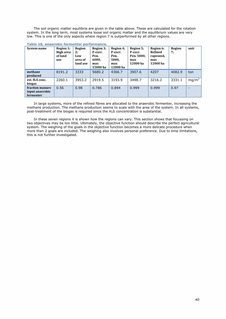
40

The soil organic matter equilibria are given in the table above. These are calculated for the rotation

system. In the long term, most systems loose soil organic matter and the equilibrium values are very low. This is one of the only aspects where region 7 is outperformed by all other regions. Table 18, anaerobic fermenter performance.

System name Region 1; High area of land use

Region 2; Low area of land use

Region 3; P-excr. Pen. 6000, max 15000 ha

Region 4; P-excr. Pen. 5000, max 12000 ha

Region 5; P-excr. Pen. 5000, max 12000 ha

Region 6; Refined rapeseed, max 12000 ha

Region 7;

unit

methane produced

8191.2 3333 5680.2 4366.7 3907.6 4207 4082.9 ton

est. H2S conc. biogas

2260.1 3953.2 2919.5 3193.9 3498.7 3216.2 3331.1 mg/m3

fraction manure input anaerobic fermenter

0.56 0.98 0.786 0.894 0.999 0.999 0.97 -

In large systems, more of the refined fibres are allocated to the anaerobic fermenter, increasing the methane production. The methane production seems to scale with the area of the system. In all systems, post-treatment of the biogas is required since the H2S concentration is substantial.

In these seven regions it is shown how the regions can vary. This section shows that focussing on

two objectives may be too little. Ultimately, the objective function should describe the perfect agricultural system. The weighing of the goals in the objective function becomes a more delicate procedure when more than 2 goals are included. The weighing also involves personal preference. Due to time limitations, this is not further investigated.

41

42

5. Discussion From the results it can be seen that the goals in the objective function have a large impact on the

optimisation. The weighing factors used for the goals also have influence. In this study, the objective function is analysed for two goals in the objective function. More goals can be added to the function if desired. The objective function is a function which describes how good a system is. To define the objective function, a good system has to be described by numbers. This leads to the question; what defines a good agricultural system? The definition of a good system differs among stakeholders. Stakeholders are separated by their expectations, believes and intentions for instance; Entrepreneurs in the region most likely want to maximize their profits. A government might want to have reasonable profits within the region but also a high total productivity or reduced pressure on the environment. Environmentalists may want sustainable production of crops and other products. While all these goals

can be transformed into objective functions, there is only 1 region which can be filled. Completely satisfying one stakeholder can result in unpleasing several others. The eventual design of such an agricultural region is a compromise between all the aspects.

During the optimisation several local minima were found. Optimisation is used as an analysis tool, rather than an optimisation tool. Therefore the local minima still provide valuable information on possible systems, as there are many reasons to prefer one system over another. Adding only two goals in the objective function allows creating a series with increasing weighing factor on one of the goals. All the data collected from these optimisations give information on system changes with regard to the objective function. When three goals are used in the optimisation, two of the weighing factors need to be changed to create such series. Changing two weighing factors increases the time required for the simulations.

5.1 Maize distribution After the data was collected, a modelling error has been found. The maize composition represents

whole plant maize, this results in very high fibre intake for pigs when the maize is distributed to pigs. Pigs are not able to digest large quantities of lignocellulose. Instead of using whole maize composition, corn-cob mix should have been used. Below is a table with the differences. In this table, the nutrients present in 1 ton dry matter whole maize plant is converted into CCM.

Table 19, whole maize plant composition compared with corn cob mix composition.

whole plant CCM

protein 0.06 0.051205 Ton

Sugar 0.39 0.347985 Ton

Lipids 0.065 0.02508 Ton

Fibres 0.38 0.01254 Ton

P 0.0019 0.001724 Ton

K 0.01 0.002142 Ton

The table shows that 1 ton DM whole maize contains 0.5225 ton DM CCM. When multiplying this with

the composition of the CCM the numbers in the table are found. The protein, sugar and P content are almost the same. The lipid, fibre and K content decrease significant. Since sugar and starch are the main source of energy, the energy requirement is hardly affected by this change. The energy yield on CCM is also higher compared to the energy yield on whole plant maize.

5.2 Area of land use From figure 9 it can be concluded that increasing the use of arable land in the system reduces the

sum of imports. This can be seen as becoming more self-sufficient. However, some imports will always be required as products leave the system for consumption and nutrients are lost in the soil. Finding the optimal design of an agricultural region involves making choices. Most of the choices have both positive and negative consequences, finding a perfect solution is unlikely. For instance increasing land use has several advantages; however additional arable land may be unavailable or expensive. Changing land into arable land decreases another type of land use, this may be undesirable.

When observing a high import system, it has to be remembered that these imports need to be produced somewhere. Land for the production of food or feed has to be used somewhere. So this can be seen as a dilemma between producing feed locally and outsourcing the feed production. When assuming

the yield of the imported feed is 8 ton DM per hectare, the imported feed can also be expressed in hectares of land used.

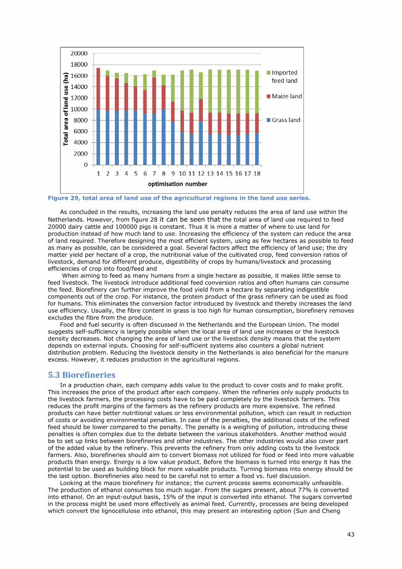
43

Figure 29, total area of land use of the agricultural regions in the land use series.

As concluded in the results, increasing the land use penalty reduces the area of land use within the

Netherlands. However, from figure 28 it can be seen that the total area of land use required to feed

20000 dairy cattle and 100000 pigs is constant. Thus it is more a matter of where to use land for production instead of how much land to use. Increasing the efficiency of the system can reduce the area

of land required. Therefore designing the most efficient system, using as few hectares as possible to feed as many as possible, can be considered a goal. Several factors affect the efficiency of land use; the dry matter yield per hectare of a crop, the nutritional value of the cultivated crop, feed conversion ratios of livestock, demand for different produce, digestibility of crops by humans/livestock and processing efficiencies of crop into food/feed and

When aiming to feed as many humans from a single hectare as possible, it makes little sense to feed livestock. The livestock introduce additional feed conversion ratios and often humans can consume the feed. Biorefinery can further improve the food yield from a hectare by separating indigestible components out of the crop. For instance, the protein product of the grass refinery can be used as food for humans. This eliminates the conversion factor introduced by livestock and thereby increases the land use efficiency. Usually, the fibre content in grass is too high for human consumption, biorefinery removes

excludes the fibre from the produce. Food and fuel security is often discussed in the Netherlands and the European Union. The model

suggests self-sufficiency is largely possible when the local area of land use increases or the livestock density decreases. Not changing the area of land use or the livestock density means that the system depends on external inputs. Choosing for self-sufficient systems also counters a global nutrient distribution problem. Reducing the livestock density in the Netherlands is also beneficial for the manure excess. However, it reduces production in the agricultural regions.

5.3 Biorefineries In a production chain, each company adds value to the product to cover costs and to make profit.

This increases the price of the product after each company. When the refineries only supply products to the livestock farmers, the processing costs have to be paid completely by the livestock farmers. This reduces the profit margins of the farmers as the refinery products are more expensive. The refined products can have better nutritional values or less environmental pollution, which can result in reduction of costs or avoiding environmental penalties. In case of the penalties, the additional costs of the refined feed should be lower compared to the penalty. The penalty is a weighing of pollution, introducing these penalties is often complex due to the debate between the various stakeholders. Another method would be to set up links between biorefineries and other industries. The other industries would also cover part of the added value by the refinery. This prevents the refinery from only adding costs to the livestock farmers. Also, biorefineries should aim to convert biomass not utilized for food or feed into more valuable products than energy. Energy is a low value product. Before the biomass is turned into energy it has the

potential to be used as building block for more valuable products. Turning biomass into energy should be the last option. Biorefineries also need to be careful not to enter a food vs. fuel discussion.

Looking at the maize biorefinery for instance; the current process seems economically unfeasible. The production of ethanol consumes too much sugar. From the sugars present, about 77% is converted into ethanol. On an input-output basis, 15% of the input is converted into ethanol. The sugars converted in the process might be used more effectively as animal feed. Currently, processes are being developed which convert the lignocellulose into ethanol, this may present an interesting option (Sun and Cheng

44

2002, Tao et al. 2011). The refining of crops is an interesting option to reduce the environmental impact

of livestock farming. During the refining of crops, often fibres are separated from sugars and protein. Often these fibres

streams still contain valuable protein. When fibres refined in the biorefineries are used for energy production a valuable resource is essentially wasted. The revenue on biogas is insufficient compared to the price of the fibres. These high fibre products of the biorefineries can be converted into building blocks for the chemical industry. The fibre stream of the grass biorefinery still contains protein. This should either be fed to cattle or extracted to avoid the loss of protein. The anaerobic fermenter performs decent when digesting manure. Another possibility is to redesign the anaerobic fermenter to extract the nutrients present in the manure and converting them into valuable fertilizer.

From the series with increasing penalty on P excretion it can be concluded that biorefinery can

reduce the P intake in livestock. In the P series, the P excretion for cattle did not change. The average annual intake of P in this series is 18.3 kg P/year per cow. This is below the recommended intake of 27 kg P per year per cow (Sehested 2004). Research by van Krimpen et al. (2009) showed an average P intake in Dutch dairy cows of 27 kg P per year, while the minimum P requirement of dairy cattle is 18 kg P/year. Van Krimpen et al. (2009) further note that no P imbalance is expected in a diet with 2.8 g P/kg DM as the absorption of P increases in lower P diets. In the land use series small systems with little refined feed, have an annual P intake of 22 kg/year per cow. Biorefinery can reduce this to 18.3 kg P/year per cow, a reduction of 16.8%. Even though all numbers are below the recommended intake of 27 kg P per year per cow, these numbers are all higher than the minimum given in van Krimpen et al. (2009).

5.4 Soil organic matter The soil organic matter in the region declines to worrying levels when the predicted equilibrium is

reached. The digestate is not able to counter the decomposition of organic matter. However, the root systems of the harvested crop should also be considered. For maize the root system can contribute between 1 and 3 ton dry matter per hectare with 90% of the roots in the top 40cm of the soil (van Schooten et al. 2013). Deru et al. (2014) found that the dry matter weight of grass roots in the top 20 cm in the soil is between 1.5 and 2 ton dry matter per hectare. This would contribute to the soil organic matter supply. Other factors affecting soil organic matter, such as erosion, are also not considered. The dilemma regarding soil organic matter must be kept in mind. Soil organic matter can be used as a carbon sink, it also functions as a fuel for important dynamics in the soil (Janzen, 2005). When in the

agricultural region, on average 2 ton dry matter is added to the soil by the root systems, the total organic matter in the soil will be 58 ton per hectare. This results in a small gain of organic matter in the soils when a 2 year grass 1 year maize rotation is used. So the organic matter in the soil appears to be fine when the added organic matter from roots is taken into account.

5.5 Biological nitrogen fixation Biological nitrogen fixation is used in the system to increase N supply to the grass soil. Most of the

systems have N limitation in grass cultivation. To achieve 10 ton dry matter grass per hectare with protein content of 210g/kg DM, 336 kg N is incorporated in the grass. Adding another 25% loss of N in

the soil, and the supply of N to the soil needs to be 448 kg N per hectare. Biological nitrogen fixes 500 ton N per year. When biological nitrogen fixation is included, the grass cultivated in the system which requires no additional N input is almost 11160 ton grass DM. This means that 1116 ha of grass land can be cultivated without the import of fertilizer. Alternatively, the additional N can result in higher grass yields from a hectare instead of reducing the fertilizer use. Areal productivity of grass alone is expected to be higher compared to grass clover systems, as the clover requires energy for fixating N. However, grass only systems still have to comply with the European fertilizer laws. BNF allows for the addition of N to the system without the N counting towards the law, combined with N being limited in most simulations, results in high benefits of BNF. In a system with 10000 ha grass, the fixation of 500 ton N would save 70 euro per hectare. The 500 ton N would otherwise have to be supplied from fertilizer N. The fertilizer contains 30% N, while the price is 420 euro per ton. Not using BNF is interesting when the system is not limited by N supply, as the profit increases more from additional grass yield than from

biological nitrogen fixation. In this study, biological nitrogen is included as the system is designed to operate within, or close to, legal maxima.

45

46

6. Conclusions A model is created which calculates the annual in- and outputs of seven companies in an agricultural

region. The companies include a grass farm, maize farm, grass refinery, maize refinery, cattle farm, pig farm and anaerobic digester. An additional model is created to simulate the soil organic matter in the region over time. The agricultural model can be supplied with a set of objectives, constraints, initial guesses and upper- and lower bounds to calculate an optimal design of the region. The optimal design of an agricultural region depends mainly on the objective function and constraints. When multiple goals are included in the objective function weighing factors allow for different emphasis on the objectives. It is shown that a series of optimisations with 2 objectives and a variable weighing factor can be valuable analysis tool. The model can predict the effect of economic and environmental policies. The model can also be used to analyse the efficiency of hypothetical agricultural regions with regard to land use,

nutrient recycling and self-sufficiency. Two series of increasing weighing factors in the objective function have been simulated. The first

series aims to maximize economic profit with an increasing penalty on the area of land use. It was found that a higher penalty on land use results in a smaller system, which required more imports thus are less self-sufficient. Furthermore it is shown that more self-sufficient systems reduce the P excretion by livestock. The second series aims to maximize economic profit with an increasing penalty on P excretion and a maximum area of land use. A penalty on P excretion increases the mass distributed to the biorefineries. The biorefineries exclude P from the cultivated crop, thereby reducing the P content of the diet. The total profit of the region does not decrease significant in this series.

The grass biorefinery is shown to have great potential, both from an economic and from an environmental point of view. The refining of grass allows pigs to consume locally produced protein. This offers more flexibility in a diet. However, the refining adds additional value to the protein which results in the decrease of the profit margins on the pig farm. With an increased focus on reducing environmental pollution such refineries are becoming attractive.

Ethanol fermentation from sugars present in maize does not appear to be an attractive solution in

agricultural regions with limited area available. In the land use series it is shown that the maize refinery hardly makes profit even when refining large quantities. Feeding the sugars to the livestock can result in more efficient systems. Refining maize is still a possibility, but the conversion of sugar into ethanol seems economically unattractive.

The study shows that a region with maize, grass and refineries can supply livestock with all the essential nutrients. Refining maize and grass reduces the amount of nutrients present in the manure, thereby reducing the manure excess in the region.

The anaerobic fermenter recovers energy from the excreted manure. The digestate produced by the

fermenter can be used as fertilizer. Supplying the soil with digestate from the anaerobic fermenter greatly improves the recycling of nutrients within the region. The digestate also has a positive effect on the soil organic matter. However, when taking only digestate into account, the soil organic matter reduces significant in long term. The digestate combined with the root systems of the plants could be sufficient to stabilize the soil organic matter. The anaerobic fermenter has a low margin of profit when the digestate is considered to be manure, as is done by the law. By considering the digestate as a fertilizer, the margins on the fermenter should increase and the overall nutrient recycling increases.

Soybean import feed is replaced by a refined rapeseed feed with high protein content. Optimisation

resulted in a shift towards more maize cultivation in the region. The total amount of import decreased in the region however the economic potential of the region also decreased.

47

48

7. Recommendations The model is based on parameters found in literature. All these parameters are fixed and are not

changed within an optimisation. A sensitivity analysis is not included in this study. The outcome of the optimisation can differ when parameters are chosen slightly different. To get insight into which parameters are important a sensitivity analysis should be performed. Some of the parameters for which the model might be sensitive include; changes in prices when the objective function includes an economic goal and the dry matter yield per hectare when area of land use is included.

From a nutritional point of view, amino acids are very important in the livestock diet. Currently the

amino acids are not included in the model, instead total protein is used. Adding the 4 most important amino acids allows further optimisation with regard to protein distribution (lysine, Methionine, Threonine

and Tryptophan for pigs (van Krimpen et al. 2010). However the distribution of amino acids over the refined products is currently unknown. Either assumptions or research is needed. Besides adding the amino acids, adding different digestibilities also allows for better optimisation with regard to protein.

The soil nutrient model is based on a steady state model. A more detailed soil model results in better

prediction for nutrients and organic matter in the soil. Detailed soil models have already been developed. These models can simulate soil organic matter as well as nutrient dynamics inside the soil. Weather effects can even be included. Such soil model would also allow a variable yield depending on several factors.

In the results it was shown that the grass biorefinery makes more profit compared to the maize

biorefinery. The maize biorefinery has a difficult time making profit at all. The fermentation results in a reduction of sugars distributed to the livestock. These sugars could be more valuable as feed instead of ethanol. When using sugar for ethanol production, there always is a feed vs. fuel discussion. Currently research is done into the conversion of lignocellulose into ethanol. This is interesting in combination with the production of corn cob mix for pigs. When producing CCM large parts of the lignocellulose are not utilized. Converting this into ethanol increases the systems’ efficiency without reducing the potential to feed animals.

Adding other crop-biorefinery combinations allows for greater study into optimal design of an

agricultural region. This adds more product- and biodiversity to the system and can make the system more productive. Other form of livestock can also be added. The main animal missing from this system is the chicken. Chickens are often found in agricultural regions as they produce eggs and meat. Other

interesting possibilities include adding fish farms or seaweed farms. For designing the most efficient agricultural system, human food requirements should be included.

When humans are included in the model, the model can be made even more efficient. When humans are introduced in the system, it makes sense to include the wastewater treatment as well as this allows recycling of nutrients excreted by humans. However, human nutritional habits can differ significant. Also, the recycling of nutrients becomes more difficult to model as not only manure ends up in the sewage system. The grass biorefinery produces a product which could be suitable for human consumption. This is the high protein product. Since the fibres are excluded this could be an interesting source for protein which is locally produced.

From a policy point of view, the model can be used to guide governmental interference. The model

can provide a basis for policy discussions and evaluation as it can calculate the effect of multiple policies in a larger region. Even better would be to discuss the objectives and constraints with various stakeholders and the government. Since the results show very different systems can be designed depending on the goal of the system. This allows for the formulation of an objective function for the optimisation which all stakeholders agree with and thus the outcomes of the optimisation have greater chance of implementation.

As mentioned in the results, personally I think region 7 in the section individual systems provides a

nice balance between profit, environment, self-sufficiency and area of land use. All these factors can be placed in the objective function, finding weighing factors which satisfy all stakeholders might prove to be difficult. However it is interesting to study how the system behaves when more objectives are

introduced. The results show the model is able to predict land change within the agricultural region and the

amount of land change required outside the system. Adding more data on the land used outside the region can result in a model which is able to predict land use change. This enables the possibility to predict the effect of various policies, biorefineries and distribution of nutrients over livestock. This could prove to be a very valuable tool for assessing biorefineries and countering deforestation in tropical regions.

49

8. Acknowledgement I would like to thank my supervisers for guiding me during my master thesis; Marja Teekens and Gerard van Willigenburg. Marja guided me with her knowledge on on agriculture. Before this thesis, agriculture was not my area of expertise. Discussing the outcomes with Marja always resulted in interesting observations and conclusions. Gerard guided me with the modelling aspect of this thesis. I specifically want to thank him for stressing how the objective function should and can be used. I would also like to thank prof. Johan Sanders, his extensive knowledge on biorefineries helped significantly during the course of this thesis. Discussions with prof. Johan Sanders and Marieke bruijns, who I also thank, on the design of the agricultural region and the interpretation of the outcomes resulted in new insights and additional possibilities. Finally, I would like to thank all the people at the BCT group for the interesting non-work related discussion during coffee and lunch breaks.

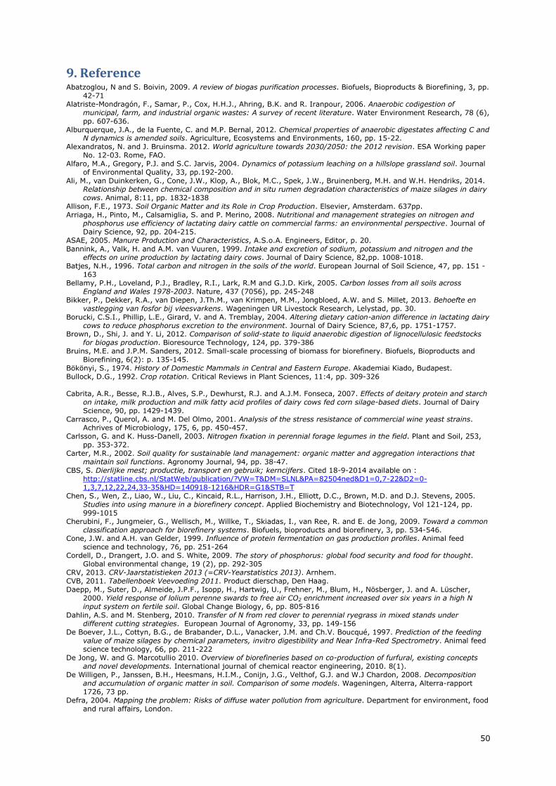
50

9. Reference Abatzoglou, N and S. Boivin, 2009. A review of biogas purification processes. Biofuels, Bioproducts & Biorefining, 3, pp.

42-71 Alatriste-Mondragón, F., Samar, P., Cox, H.H.J., Ahring, B.K. and R. Iranpour, 2006. Anaerobic codigestion of

municipal, farm, and industrial organic wastes: A survey of recent literature. Water Environment Research, 78 (6), pp. 607-636.

Alburquerque, J.A., de la Fuente, C. and M.P. Bernal, 2012. Chemical properties of anaerobic digestates affecting C and N dynamics is amended soils. Agriculture, Ecosystems and Environments, 160, pp. 15-22.

Alexandratos, N. and J. Bruinsma. 2012. World agriculture towards 2030/2050: the 2012 revision. ESA Working paper No. 12-03. Rome, FAO.

Alfaro, M.A., Gregory, P.J. and S.C. Jarvis, 2004. Dynamics of potassium leaching on a hillslope grassland soil. Journal of Environmental Quality, 33, pp.192-200.

Ali, M., van Duinkerken, G., Cone, J.W., Klop, A., Blok, M.C., Spek, J.W., Bruinenberg, M.H. and W.H. Hendriks, 2014. Relationship between chemical composition and in situ rumen degradation characteristics of maize silages in dairy cows. Animal, 8:11, pp. 1832-1838

Allison, F.E., 1973. Soil Organic Matter and its Role in Crop Production. Elsevier, Amsterdam. 637pp. Arriaga, H., Pinto, M., Calsamiglia, S. and P. Merino, 2008. Nutritional and management strategies on nitrogen and

phosphorus use efficiency of lactating dairy cattle on commercial farms: an environmental perspective. Journal of Dairy Science, 92, pp. 204-215.

ASAE, 2005. Manure Production and Characteristics, A.S.o.A. Engineers, Editor, p. 20. Bannink, A., Valk, H. and A.M. van Vuuren, 1999. Intake and excretion of sodium, potassium and nitrogen and the

effects on urine production by lactating dairy cows. Journal of Dairy Science, 82,pp. 1008-1018. Batjes, N.H., 1996. Total carbon and nitrogen in the soils of the world. European Journal of Soil Science, 47, pp. 151 -

163 Bellamy, P.H., Loveland, P.J., Bradley, R.I., Lark, R.M and G.J.D. Kirk, 2005. Carbon losses from all soils across

England and Wales 1978-2003. Nature, 437 (7056), pp. 245-248 Bikker, P., Dekker, R.A., van Diepen, J.Th.M., van Krimpen, M.M., Jongbloed, A.W. and S. Millet, 2013. Behoefte en

vastlegging van fosfor bij vleesvarkens. Wageningen UR Livestock Research, Lelystad, pp. 30. Borucki, C.S.I., Phillip, L.E., Girard, V. and A. Tremblay, 2004. Altering dietary cation-anion difference in lactating dairy

cows to reduce phosphorus excretion to the environment. Journal of Dairy Science, 87,6, pp. 1751-1757. Brown, D., Shi, J. and Y. Li, 2012. Comparison of solid-state to liquid anaerobic digestion of lignocellulosic feedstocks

for biogas production. Bioresource Technology, 124, pp. 379-386 Bruins, M.E. and J.P.M. Sanders, 2012. Small-scale processing of biomass for biorefinery. Biofuels, Bioproducts and

Biorefining, 6(2): p. 135-145. Bökönyi, S., 1974. History of Domestic Mammals in Central and Eastern Europe. Akademiai Kiado, Budapest. Bullock, D.G., 1992. Crop rotation. Critical Reviews in Plant Sciences, 11:4, pp. 309-326 Cabrita, A.R., Besse, R.J.B., Alves, S.P., Dewhurst, R.J. and A.J.M. Fonseca, 2007. Effects of deitary protein and starch

on intake, milk production and milk fatty acid profiles of dairy cows fed corn silage-based diets. Journal of Dairy Science, 90, pp. 1429-1439.

Carrasco, P., Querol, A. and M. Del Olmo, 2001. Analysis of the stress resistance of commercial wine yeast strains. Achrives of Microbiology, 175, 6, pp. 450-457.

Carlsson, G. and K. Huss-Danell, 2003. Nitrogen fixation in perennial forage legumes in the field. Plant and Soil, 253, pp. 353-372.

Carter, M.R., 2002. Soil quality for sustainable land management: organic matter and aggregation interactions that maintain soil functions. Agronomy Journal, 94, pp. 38-47.

CBS, S. Dierlijke mest; productie, transport en gebruik; kerncijfers. Cited 18-9-2014 available on : http://statline.cbs.nl/StatWeb/publication/?VW=T&DM=SLNL&PA=82504ned&D1=0,7-22&D2=0-1,3,7,12,22,24,33-35&HD=140918-1216&HDR=G1&STB=T

Chen, S., Wen, Z., Liao, W., Liu, C., Kincaid, R.L., Harrison, J.H., Elliott, D.C., Brown, M.D. and D.J. Stevens, 2005. Studies into using manure in a biorefinery concept. Applied Biochemistry and Biotechnology, Vol 121-124, pp. 999-1015

Cherubini, F., Jungmeier, G., Wellisch, M., Willke, T., Skiadas, I., van Ree, R. and E. de Jong, 2009. Toward a common classification approach for biorefinery systems. Biofuels, bioproducts and biorefinery, 3, pp. 534-546.

Cone, J.W. and A.H. van Gelder, 1999. Influence of protein fermentation on gas production profiles. Animal feed science and technology, 76, pp. 251-264

Cordell, D., Drangert, J.O. and S. White, 2009. The story of phosphorus: global food security and food for thought. Global environmental change, 19 (2), pp. 292-305

CRV, 2013. CRV-Jaarstatistieken 2013 (=CRV-Yearstatistics 2013). Arnhem. CVB, 2011. Tabellenboek Veevoeding 2011. Product dierschap, Den Haag. Daepp, M., Suter, D., Almeide, J.P.F., Isopp, H., Hartwig, U., Frehner, M., Blum, H., Nösberger, J. and A. Lüscher,

2000. Yield response of lolium perenne swards to free air CO2 enrichment increased over six years in a high N input system on fertile soil. Global Change Biology, 6, pp. 805-816

Dahlin, A.S. and M. Stenberg, 2010. Transfer of N from red clover to perennial ryegrass in mixed stands under different cutting strategies. European Journal of Agronomy, 33, pp. 149-156

De Boever, J.L., Cottyn, B.G., de Brabander, D.L., Vanacker, J.M. and Ch.V. Boucqué, 1997. Prediction of the feeding value of maize silages by chemical parameters, invitro digestibility and Near Infra-Red Spectrometry. Animal feed science technology, 66, pp. 211-222

De Jong, W. and G. Marcotullio 2010. Overview of biorefineries based on co-production of furfural, existing concepts and novel developments. International journal of chemical reactor engineering, 2010. 8(1).

De Willigen, P., Janssen, B.H., Heesmans, H.I.M., Conijn, J.G., Velthof, G.J. and W.J Chardon, 2008. Decomposition and accumulation of organic matter in soil. Comparison of some models. Wageningen, Alterra, Alterra-rapport 1726, 73 pp.

Defra, 2004. Mapping the problem: Risks of diffuse water pollution from agriculture. Department for environment, food and rural affairs, London.

51

Delgado, C., Rosegrant, M., Steinfeld, H., Ehui, S. and C. Courbois, 2002. Livestock to 2020: The next food revolution. 2020 Vision for Food, Agriculture, and the Environment. Discussion Paper 28.

Deru, L., van Eekeren, N. and de Boer, 2014. Rooting density of three grass species and eight lolium perenne cultivars. Grassland science in Europe, 17, pp. 604-606.

Diacono, M. and F. Montemurro, 2010. Long-term effects of organic amendments on soil fertility. A review. Agronomy for sustainable development, 30, pp. 401-422.

Drackley, J.K., Donkin, S.S. and C.K. Reynolds, 2006. Major advances in fundamental dairy cattle nutrition. Journal of Dairy Science, 89 (4), pp. 1324-1336.

Duke, J.A., 1983. Handbook of energy crops. Unpublished, available on: https://www.hort.purdue.edu/newcrop/duke_energy/Lolium_perenne.html

Dumanski, J., 2004. Carbon sequestration, soil conservation, and the Kyoto Protocol: summary of implications. Climatic Change 65, 255–261.

Eastridge, M.L., 2006. Major advances in applied dairy cattle nutrition. Journal of Dairy Science, 89, pp. 1311-1323. EC, 2004. Towards a European knowledge based bioeconomy: workshop conclusions on the use of plant biotechnology

for the production of biobased product. Luxembourgh, Office for Official Publications of the European Communities. EEA, 2013. Environmental indicators report 2013: Natural resources and human well-being in a green economy.

Luxembourg. Publications Office of the European Union. Epstein, j. and M. Bichard, 1984. in Evolution of Domesticated Animals. I. L. Mason, Ed. Longman, New York, pp. 145–

162. EUBIA. About Biomass pelleting: Economics, applications and standards. Accessed on: 07-05-2015, Available from: http://www.eubia.org/index.php/about-biomass/biomass-pelleting/economics-applications-and-standards Faostat http://faostat3.fao.org/browse/Q/*/E Fillaudeau, L., Blanpain-Avet, P. and G. Daufin, 2006. Waste, wastewater and waste management in brewing

industries. Journal of Cleaner Production, 14, pp. 463-471. Filya, I., 2004. Nutritive value and aerobic stability of whole crop maize silage harvested at four stages of maturity.

Animal feed science and technology, 166, pp. 141-150 Finke, C., Möller, k., Schlink, S., Gerowitt, B. and J. Isselstein, 1999. The environmental impacts of maize cultivation in

the European Union: Practical options for the improvement of the environmental impact. Case study Germany. Research Centre for agriculture and environment.

Fleming, R. and M. Ford, 2001. Human versus animals-comparison of waste properties. Ridgetown College, University of Guelph.

Fraser, D., 2005. Animal welfare and the intesificationof animal production. Food and Agriculture Organization of the United Nations, rome, pp. 28. ISBN 92-5-105386-3

Fuchs, W. and B. Drosg, 2013. Assessment of the state of the art of technologies for the processing of digestate residue from anaerobic digesters. Water Science & Technology, 67, 9, pp. 1984-1993.

Gallaghan, F.J., Wase, D.A.J., Thayanithy, K. and C.F. Forster, 1999. Co-digestion of waste organic solids: Batch studies. Bioresource Technology, 67, pp. 117-122.

Geels, F.W., 2009. Foundational ontologies and multi-paradigm analysis, applied to the socio-technical transistion from mixed farming to intensive pig husbandry (1930-1980). Technology Analysis & Strategic Management, 21(7), pp. 805-832.

Giller, K.E., Beare, M.H., Lavelle, P., Izac, M.N. and M.J. Swift, 1997. Agricultural intensification, soil biodiversity and agroecosystem function. Applied Soil Ecology, 6, pp. 3-16

Goldemberg, J. and P. Guardabassi, 2009. Are biofuels a feasible option? Energy Policy, 37(1), p. 10-14. Grieder, C., Mittweg, G., Dhillon, B.S., Montes, J.M., Orsini, E. and A.E. Melchinger, 2012. Kinetics of methane

fermentation yield in biogas reactors: genetic variation and association with chemical composition in maize. Biomass and Bioenergy, 37, pp. 132-141

Groenendijk, P., Renaud, L.V., and J. Roelsma, 2005. Prediction of Nitrogen and Phosphorus leaching to groundwater and surface waters; Process descriptions of the animo4.0 model. Alterra, Report 983, Wageningen.

Halvorson, A.D. and C.P. Jantalia, 2011. Nitrogen fertilization effects on irrigated no-till corn production and soil carbon and nitrogen. Agronomy journal, 103 (3), pp. 1423-1431.

Hart, M.R., Quin, B.F. and M.L. Nguyen, 2004. Phosphorus runoff from agricultural land and direct fertilizer effects: A review. Journal of Environmental Quality, 33, pp. 1954-1972.

Hilliard, E.P., Beard, J. and G.R. Pearce, 1979. Utilization of piggery waste I. the chemical composition and in vitro organic matter digestibility of pig faeces from commercial piggeries in south eastern Australia. Agriculture and Environment, 4, pp. 171-180.

Hindrichsen, I.K., Kreuzer, M., Madsen, J. and K.E. Bach Knudsen, 2006. Fiber and lignin analysis in concentrate, forage, and feces: detergent versus enzymatic-chemical method. Journal of Dairy Sciences, 89 (6), pp. 2168-2176

Hoover, S.R. and N. Porges (1952). Assimilation of dairy wastes by activated sludge II: the equation of synthesis and oxygen utilization. Journal Water Pollution Control Federation, 49, p.768

IEA Bioenergy, 2009. Biorefineries: adding value to the sustainable utilisation of biomass. IEA Bioenergy Task 42: Biorefineries, pp. 16.

IEA Bioenergy, 2014. Task 37 country overview. IEA Bioenergy task 37, p. 32 Jarvis, s., Hutchings, N., Brentrup, F., Olesen, J.E. and K.W. van de Hoek. In: The European Nitrogen Assessment, ed.

M.A. Sutton, C.M. Howard, J.W. Erisman, G. Billen, A. Bleeker, P. Grennfelt, H. van Grinsven and B. Grizzetti. Published by Cambridge University Press. © Cambridge University Press 2011, European

union. Jančík, F., Koukolová, V. and P. Homolka, 2010. Ruminal degradability of dry matter and neutral detergent fibre of

grasses. Czech journal of animal sciences, 55 (9), pp 359-371 Janzen, H.H., 2005. The soil carbon dilemma: Shall we hoard it or use it? Soil Biology & Biochemistry, 36, pp. 419-424 Johnston, A.E., Poulton, P.R. and K. Coleman, 2009. Soil organic matter: its importance in sustainable agriculture and

carbon dioxide fluxed. Advances in Agronomy, 101, pp. 1-57. Karlen, D.L., Varvel, G.E., Bullock, D.G. and R.M Cruse, 1994. Crop rotations for the 21st century. Advances in

Agronomy, 53, pp. 1-45 Kiers, J.L., Nout, R.M.J. and F.M. Rombouts, 2000. In vitro digestibility of processed and fermented soya bean, cowpea

and maize. Journal of the Science of Food and Agriculture, 80, pp. 1325-1331. Klop, A., de Jonge, L.H. and G.G. Brandsma, 2008. Eiwitwaarde vers gras. Animal Sciences Group: Wageningen.

52

Kohn, R.A., Dinneen, M.M. and E. Russek-Cohen, 2005. Using blood urea nitrogen to predict nitrogen excretion and efficiency of nitrogen utilization in cattle, sheep, goats, horses, pigs and rats. Journal of Animal Science, 83, pp. 879-889.

Lal, R., 2002. Why carbon sequestration in agricultural soils?. In: Kimble, J.M., Lal, R., Follett, R.F. (Eds.), Agricultural Practices and Policies for Carbon Sequestration in Soil. Lewis Publishers/CRC Press, London/Boca Raton, FL, pp. 21–30.

Lal, R., 2004. Soil carbon sequestration impacts on global climate change and food security. Science 304, 1623–1627. Langeveld, H., Meeusen, M. and J. Sanders [ed.], 2010. The biobased economy: Biofuels, materials and chemicals in

the post-oil era. London, Earthscan, ISBN 978-1-84407-770-0. Larkin, D.M., 2011. Status of the cattle genome map. Cytogenetic and Genome Research, 134, pp. 1-8. Latifian, M., Liu, J. and Mattiasson, B., 2012. Struvite-based fertilizer and its physical and chemical properties.

Environmental technology. Vol. 33 (24), p. 2691–2697 LEI, 2013. BINternet, Farm Accountancy Data Network. Available on:

http://www3.lei.wur.nl/binternet_asp/Index.aspx?Database=LTC&language=1 Liao, W., Wen, Z., Hurley, S., Liu, Y., Liu, C. and S. Chen, 2005. Effects of hemicellulose and lignin on enzymatic

hydrolysis of cellulose from dairy manure. Applied Biochemistry and Biotechnology, 121-124, pp. 1017-1030. Lobe, I., Du Preez, C.C and W. Amelung, 2002. Influence of prolonged arable cropping on lignin compounds in sandy

soils of the South African Highveld. European journal of soil science, 53, pp. 553-562. Lu, Y.C., Watkins, K.B., Teasdale, J.R and A.A. Abdul-Baki, 2000. Cover crops in sustainable food production. Food

review international, 16, 2, pp. 121-157. Liu Y.G., Zhou M.Q. and M.L. Liu, 1994. A survey of nutrients and toxic factors in commercial rapeseed in China and

evaluation of detoxification by water extraction. Animal feed science and technology, 45, pp. 257 – 270. Lund, B., Jensen, V.F., Have, P. and B. Ahring, 1996. Inactivation of virus during anaerobic digestion of manure in

laboratory scale biogas reactors. Antonie van Leeuwenhoek, 69, pp. 25-31. Magidan, M.t., Martinko, J.M., and J. parker (1999). Brock Biology of microorganisms, 8th ed., Prentice-Hall, Upper

Saddle River, NJ Malezieux E, Crozat Y, Dupraz C, Laurans M, Makowski D, Ozier-Lafontaine H, Rapidel, B., de Tourdonnet, S. and M.

Valentin-Morison, 2009. Mixing plant species in cropping systems: concepts, tools and models. A review. Agronomy for Sustainable Development, 29, pp. 43-62

Malhi, S.S., Lemke, R., Wang, Z.H., Baldev, S. and B.S. Chhabra, 2006. Tillage, nitrogen and crop residue effects on crop yield, nutrient uptake, soil quality, and greenhouse gas emissions. Soil & Tillage research, 90, pp. 171-183.

McDonald, P., Henderson, A.R. and S.J.E Heron, 1991. Microorganisms. In: McDonald, P., Henderson, A.R., Heron, S.J.E. (Eds.), The Biochemistry of Silage, 2nd ed. Chalcombe Publications, Aberystwyth, UK, pp. 81–151 (Chapter 4).

McNeill, A. and M. Unkovich, in: Nutrient cycling in terrestrial ecosystems, 2007. Ed. P. Marschner and Z. Rengel. Springer-Verlag, Berlin, Heidelberg. ISBN 978-3-540-68026-0.

Mekonnen, M. and A. Hoekstra, 2010. The green, blue and grey water footprint of farm animals and animal products. Melkvee, 2014. Grassa van eigen erf. (6) june 2014, available on: http://grassa.nl/wp-

content/uploads/2014/07/Grassa-van-eigen-erf.pdf Metcalf & Eddy., Tchobanoglous, G., Burton, F. L. 1., & H. D. Stensel, (2004). Wastewater engineering: Treatment and

reuse (4th ed. International edition). Boston: McGraw-Hill. ISBN: 007-124140-X Metherell, A.K., Harding, L.A., Cole, C.V. and W.J. Parton, 1993. CENTURY soil organic matter model environment.

Technical document. Colorado State University, available on: https://www.nrel.colostate.edu/projects/century/MANUAL/html_manual/man96.html

Mińkowski, K., 2002. Influence of dehulling of rape seeds on chemical composition of meal. Animal feed science and technology, 96, pp. 237 – 244.

Molinuevo-Salces, B., Gómez, X., Morán, A. and M.C. Garía-González, 2013. Anaerobic co-digestion of livestock and vegetable processing wastes: Fibre degradation and digestate stability. Waste Management, 33, pp. 1332-1338.

Møller, H.B., Moser, V., Brask, M., Weisbjerg, M.R. and P. Lund, 2014. Feces composition and manure derived methane yield from dairy cows: influence of diet with focus on fat supplement and roughage type. Atmospheric Environment, 94, pp. 36-43.

Nadeua, E., Englund, E. and A.H. Gustafsson, 2007. Nitrogen efficiency of dairy cows as affected by diet and milk yield. Livestock Science 111, pp. 45-56.

Nasir, I.M., Ghazi, T.I.M., Omar, R. and A. Idris, 2014. Biorector performance in the anaerobic digestion of cattle manure: A review. Energy Sources, Part A: Recovery, Utilization, and Environmental Effects, 36(13), pp. 1476-1483

OECD, 2009. The Bioeconomy to 2030: designing a policy agenda. OECD, Paris, ISBN 978-92-64-03853-0 Patriche, C.V., Pîrnău, R.G., Roşca, B. and L. Stoica, 2012. Assessment of soil erosion and its impact on humus spatial

and temporal dynamics. Study case: Dobrovăţ Basin (Eastern Romania). Bulletin UASVM Agriculture, 69(1), pp. 185-194.

Pearce, G.R., 1977. Generation and utilization of wastes from intensive piggeries. 48th ANZAAS Congress, Melbourne, Aug., 1977.

Peck, M.W. and F.R. Hawkes, 1987. Anaerobic digestion of cattle slurry in an upflow anaerobic filter. Biomass, 13, pp. 125-133.

Peu, P., Picard, S., Diara, A., Girault, R., Béline, F., Bridoux, G and P. Dabert, 2012. Prediction of hydrogen sulphide production during anaerobic digestion of organic substrates. Bioresource Technology, 121, pp. 419-424

Pinxterhuis, J.B., de Boer, H.C., van Eekeren, N.J.M. and M.W.J. Stienzen, 2013. Integrating maize and triticale in grass/clover based dairy systems: examining yields and autumn soil nitrate levels. Proceedings of the New Zealand Grassland Association, 75, pp. 251-256.

Powlson, D.S., Gregory, P.J., Whalley, W.R., Quinton, J.N., Hopkins, D.W., Whitmore, A.P., Hirsch, P.R. and K.W.T Goulding, 2011. Soil management in relation to sustainable agriculture and ecosystem services. Food Policy, 36, pp. S72-S87.

Platts, 2015. Platts ethanol T2 FOB rotterdam barge (eur/cu m): 16 dec, 2013 – 14 mar, 2014. Accessed on 07-05-2015, availeble from: http://www.platts.com/news-feature/2014/agriculture/ethanol-market-update/ethanol-europe

53

Rasmussen, K.J., 1999. Impact of ploughless soil tillage on yield and soil quality: A Scandinavian review. Soil & Tillage Research, 53, pp. 3-14.

Raussi, S., 2003. Human-cattle interactions in group housing. Applied Animal Behaviour Science, 80, pp. 245-262. Reijneveld, A., van Wensem, J. and O. Oenema, 2009. Soil organic carbon contents of agricultural land in the

netherlands between 1984 and 2004. Geoderma, 152, pp. 231-238 Remmelink, G., van Dooren, H.J., van Middelkoop, J., Ouweltjes, W. and H. Wemmenhove, 2013. Handboek

Melkveehouderij 2013 (=handbook dairy farming 2013).Wageningen University live stock research, Lelystad. Sahlström, L., 2003. A review of survival of pathogenic bacteria in organic waste used in biogas plants. Bioresource

technology, 87, pp. 161-166. Sanders, J.P.M. and J.H. van Kasteren, 2010. Mest als waardevolle grondstof : enkele technologische opties.

InnovatieNetwerk: Utrecht. p. 29. Sauvant, D., Perez, J.M. and G. Tran, 2002. Tables of composition and nutritional value of feed materials. Institut

national de la recherche agronomique, Paris. Schnepf, R and B. Yacobucci, 2013. Renewable Fuel standard (RFS): Overview and Issues. Congressional Research

Service, 7-5700, R40155, p. 31. Scholz, R.W. and F.W. Wellmer, 2013. Approaching a dynamic view on the availability of mineral resources: What we

may learn from the case of phosphorus? Global environmental change, 23, pp. 11-27. Schröder, J.J., Smit, A.L., Cordell, D. and A. Rosemarin, 2011. Improved phosphorus use efficiency in agriculture: A

key requirement for its sustainable use. Chemosphere, 84, pp. 822-831. Schoumans, O.F. and P. Groenendijk, 2000. Modeling soil phosphorus levels and phosphorus leaching from agricultural

land in the Netherlands. Journal of Environmental Quality, 29, pp. 111-116. Sebek, L.B.J. and E.H.M. Temme, 2009. De humane eiwitbehoefte en eiwitconsumptie en de omzetting van plantaardig

eiwit naar dierlijk eiwit (=Human protein requirements and protein intake and the conversion of vegetable protein into animal protein). Animal Sciences Group, Wageningen UR: Lelystad. p. 19.

Sehested, J., 2004. Feeding phosphorus (P) to cattle: A new basis for Nordic recommendations. Acta Agriculturae Scandinavica, Section A — Animal Science, 54:4, pp. 169-180

Smil V. 2001. Enriching the Earth. MIT Press, Cambridge, MA. Smit, H.J., Tas, B.M., Taweel, H.Z., Tamminga, S. and A. Elgersma, 2006. Effects of perennial ryegrass (Lolium

perenne L.) cultivars on herbage production, nutritional quality and herbage intake of grazin dairy cows. Grass and Forage Science, 60, pp. 297-309

Smith, L.W. 1973. Nutritive evaluations of animal manures. Symposium:processing agricultural and municipal wastes. George E. Inglett (Ed.). Avi. Publ. Co., Westport, CT.

SoCo project team, 2009. Addressing soil degradation in EU agriculture: relevant processes, practises and policies. European communities, Luxembourg.

Stafford, D.A., Hawkes, D.L. and R. Horton, 1980. Methane production from waste organic matter. University of Michigan, CRC Press

Stanogias, G.B. and G.R. Pearce, 1987. The effect of composition on diet digestibility by pigs and on the biodegradability of the resulting pig faeces. Biological Wastes, 21, pp. 101-110.

Strudley, M.W., Green, T.R. and J.C. Ascough II, 2208. Tillage effects on soil hydraulic properties in space and time: State of the science. Soil & Tillage Research, 99, pp. 4-48.

Sukkel, W., van Geel, W. and J.J. de haan, 2008. Carbon sequestration in organic and conventional managed soils in the Netherlands. 16th IFOAM Organic World Congress, Modena, Italy

Sullivan, P., 2003. Overview of cover crops and green manures. ATTRA obtained from: http://www.moissonquebec.com/documents/cover-crops.pdf on 31-10-14.

Sun, Y. and J. Cheng, 2002. Hydrolysis of lignocellulosic material for ethanol production: a review. Bioresource Technology, 83, pp. 1-11.

Tambone, F., Genevini, P., D’Imporzano, G. and F. Adani, 2009. Assessing amendment properties of digestate by studying the organic matter composition and degree of biological stability during the anaerobic digestion of the organic fraction of MSW. Bioresource technology, 100, pp. 3140-3142.

Tao, L., Aden, A., Elander, R.T., Pallapolu, V.R., Lee, Y.Y., Garlock, R.J., Balan, V., Dale, B.E., Kim, Y., Mosier, N.S., Ladisch, M.R., Falls, M., Holtzapple, M.T., Sierra, R., Shi, J., Ebrik, M.A., Redmont, T., Yang, B., Wyman, C.E., Hames, B., Thomas, S. and R.E. Warner, 2011. Process and technoeconomic analysis of leading pretreatment technologies for lignocellulosic ethanol production using switchgrass. Bioresource technology, 102, pp. 11105-11114.

Tuesorn, S., Wongwilaiwalin, S., Champreda, V., Leethochawalit, M., Nopharatana, A., Techkarnjanaruk, S. and P. Chaiprasert, 2013. Enhancement of biogas production from swine manure by a lignocellulolytic microbial consortium. Bioresource Technology, 144, pp. 579-586.

Theunissen, B., 2012. Breeding for nobility or for production?: Cultures of dairy cattle breeding in the Netherlands, 1945-1995. ISIS, 103 (2), pp. 278-309

Thomsen, I.K., Oleson, J.E., Møller, H.B., Sørensen, P. and B.T. Christensen, 2013. Carbon dynamics and retention in soil after anaerobic digestion of dairy cattle feed and faeces. Soil Biology and Biochemistry, 58, pp. 82-87.

Tilman, D., Cassman, K., Matson, P., Naylor, R. and S. Polasky, 2002. Agricultural sustainability and intensive production practices. Nature, 418, pp. 671-677

USGS, 2013. Mineral commodity summaries 2013. U.S. Geological Survey, U.S. Government Printing Office, 198 p, ISBN 978–1–4113–3548–6

USDA, 2013. Agricultural projections to 2022. Office of the Chief Economist, World Agricultural Outlook Board, U.S. Department of Agriculture. Prepared by the Interagency Agricultural Projections Committee. Long-term Projections Report OCE-2013-1, 105 pp.

van Krimpen, M., van Middelkoop, J., Sebek, L., Jongbloed, A. and W. de Hoop, 2010. Effect van fosforverlaging in melkveerantsoenen en varkensvoeders op fosfaat excretie via de mest. Wageningen UR Livestock Research, Lelystad. Pp. 63.

van Schooten, H.A., Philipsen, A.P. and J.A.M. Groten, 2013. Handboek snijmaïs. Wageningen UR Livestock Research: Lelystad.

van Velzen, A.F.M., 1979. Adaptation of methanogenic sludge to high ammonia-nitrogen concentrations. Water Research, 13, pp. 995-999

54

van Vuuren, D.P., Bouwman, A.F. and A.H.W. Beusen, 2010. Phosphorus demand for the 1970-2100 period: A scenario of analysis of resource depletion. Global Environmental Change, 20, pp. 428-439.

Van-Camp. L., Bujarrabal, B., Gentile, A-R., Jones, R.J.A., Montanarella, L., Olazabal, C. and S-K. Selvaradjou, 2004. Reports of the Technical Working Groups Established under the Thematic Strategy for Soil Protection. EUR 21319 EN/3, 872 pp. Office for Official Publications of the European Communities, Luxembourg.

Vaneeckhaute, C., Meers, E., Michels, E., Buysse, J. and F.M.G. Tack, 2013a. Ecological and economic benefits of application of bio-based mineral fertilizers in modern agriculture. Biomass and Bioenergy, 49, pp. 239-248.

Vaneeckhaute, C., Meers, E., Michels, E., Ghekiere, G., Accoe, F. and F.M.G. Tack, 2013b. Closing the nutrient cycle by using bio-digestion waste derivatives as syntheric fertilizer substitutes: A field experiment. Biomass and Bioenergy, 55, pp. 175-189.

Veillette, m., Girard, M., Viens, P., Brzezinske, R. and M. Heitz, 2012. Function and limits of biofilters for the removal of methane in exhaust gases from the pig industry. Applied Microbiology and Biotechnology, 94, pp. 601-611.

Verbaanderd, J., 2013. Biorefinery in food production chains: Design, Modelling and optimization. MSc. Wagningen UR. Waksman, S.A., 1936. Humus: Origin, Chemical Composition, and Importance in Nature. The Williams & Wilkins

Company, Baltimore. 494 pp. Wander, M., Nissen, T., 2004. Value of soil organic carbon in agricultural lands. Mitigation and Adaptation Strategies

for Global Change 9, 417–431. Ward, A.J., Hobbs, P.J., Holliman, P.J and D.L. Jones, 2008. Optimisation of the anaerobic digestion of agricultural

resources. Bioresource Technology, 99, pp. 7928-7940. Ward, D. and K. McKague, 2007. Water requirements of livestock, F.a.R.A. Ontario Ministr of Agriculture Weber, C.L. and H.S. Matthews, 2008. Food-Miles and the relative climate impacts of food choices in the United States.

Environmental science and technology, 42 (10), pp. 3508-3513 Weiland, P., 2010. Biogas production: current state and perspectives. Applied microbiology and biotechnology, 85 (4),

p. 849-860. Wilkins, P.W., 1989. Genotype/harvesting frequency and genotype/nitrogen level interactions for annual dry matter

yield in lolium perenne in relation to breeding. Euphytica, 41, pp. 207-214. Wong, M.T.F., van der Kruijs, A.C.B.M. and A.S.E. Juo, 1992. Leaching loss of calcium, magnesium, potassium and

nitrate derived from soil, lime and fertilizers as influenced by urea applied to undisturbed lysimeters in south-east Nigeria. Fertilizer Research, 31, pp. 281-289.

Wu, l. and M.B. McGechan, 1998. A review of carbon and nitrogen processes in four soil nitrogen dynamics models. Journal of Agricultural Engineering Research, 69, 4, pp. 279-305.

Xu, L. and L.L. Diosady, 2002. The removal of phenolic compounds for the production of high-quality canola protein isolates. Available: http://chem-eng.utoronto.ca/~diosady/xulpaper.html, [10 December 2013].

Zegada-Lizarazu, W. and A. Monti, 2011. Energy crops in rotation. A review. Biomass and Bioenergy, 35, pp. 12-25 Zhang, Y., Kennedy, J.F. and C.J. Knill, 1996. Kinetic analysis of ethanol production from glucose fermentation by yeast

cells immobilized onto ceramic supports. Journal of Biomaterials Science, Polymer Edition, 7(12), pp. 1119-1126.

55

56

Appendix I. Calculation energy and protein requirement for cows The calculation is performed according to handbook melkveehouderij (remmelink et al. 2013). The FPCM, fat and milk corrected milk, can be calculated according the formula below.

𝐹𝑃𝐶𝑀 = (0.337 + 0.116 ∗ %𝑓𝑎𝑡 + 0.06 ∗ %𝑝𝑟𝑜𝑡𝑒𝑖𝑛) ∗ 𝑑𝑎𝑖𝑙𝑦 𝑚𝑖𝑙𝑘 𝑝𝑟𝑜𝑑𝑢𝑐𝑡𝑖𝑜𝑛 The average Dutch cow produces 31 l/day (CVR 2013). Milk with 4% fat and 3.3% protein has a FPCM value of 30.96. During lactation the energy (in VEM, a Dutch unit for energy requirement in animals) and protein (gDVE, gram digestible protein/day) requirement for the cow can be calculated with:

𝑉𝐸𝑀 = (5323 + 440 ∗ 𝐹𝑃𝐶𝑀 + 0.73 ∗ 𝐹𝑃𝐶𝑀2) 𝑔𝐷𝑉𝐸 = 119 + (1.396 ∗ 𝐸 + 0.000195 ∗ 𝐸2)

With E, the milk protein production in g/day, this results in 19.665 VEM and 1.874 per cow per day during lactation. Annually, a dairy cow lactates 280 days per year (CVR 2013), during the remain days, the cow needs maintenance energy and protein of 5323 VEM and 119 gDVE respectively. For maintenance, a single cow requires 452455 VEM and 10115 gDVE per year. During the 6th month of pregnancy, the cow needs an additional 450 VEM and 60 gDVE per day, totalling

to 13500 VEM and 1800 gDVE. During the 7th month of pregnancy, the cow needs an additional 850 VEM and 105 gDVE per day, totalling to 26350 VEM and 3255 gDVE. During the 8th month of pregnancy, the cow needs an additional 1500 VEM and 180 gDVE per day, totalling to 45000 VEM and 5580 gDVE. During the 9th month of pregnancy, the cow needs an additional 2700 VEM and 280 gDVE per day, totalling to 83700 VEM and 8680 gDVE. So the annual total accumulates to: Energy: 19665*280+452455+45000+83700+13500+26350=6127205 VEM per year. Protein: 1874*280+10115+5580+8680+1800+3255= 553970 gDVE per year.

VEM (‘=voeder eenheid melk’) is a Dutch relative energy unit, with 1 kg barley = 1000 VEM. 1 kg barley contains 6.9 MJ Net Energy lactation, NEL. NEL is an energy value of a feed used to estimate the maintenance and milk production. Thus 1000 VEM = 6.9 MJ NEL. So in SI units, the annual totals become: Energy: 42.3 GJ/year/cow Protein: 554 kg protein/year/cow. For all 20.000 cows this is: Energy: 846.000 GJ per year Protein: 11080 ton digestible protein per year

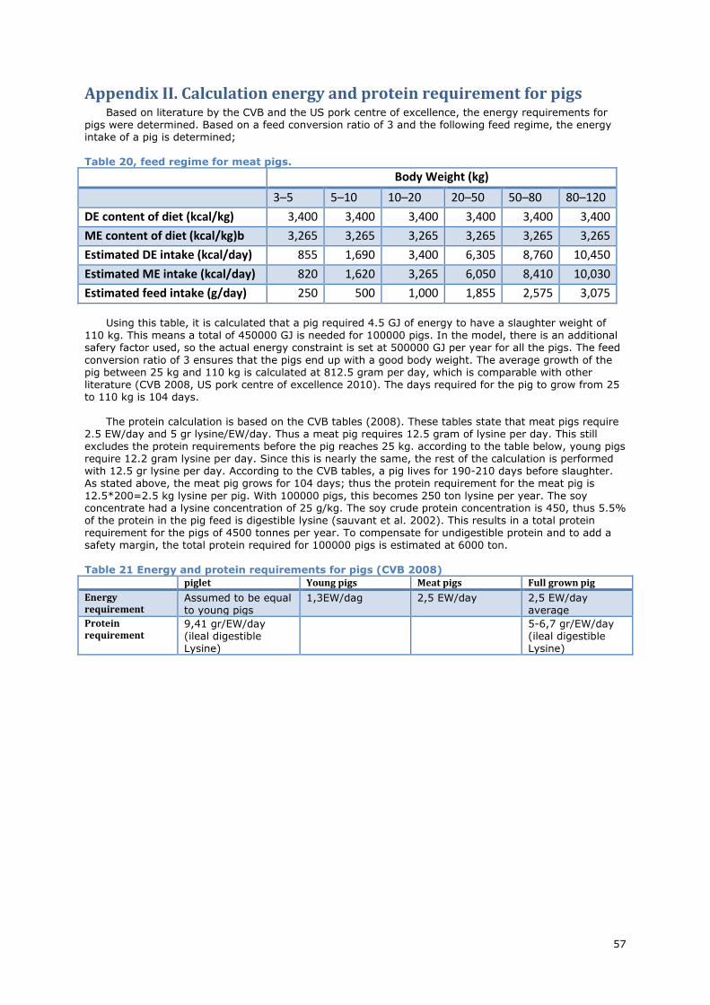
57

Appendix II. Calculation energy and protein requirement for pigs Based on literature by the CVB and the US pork centre of excellence, the energy requirements for

pigs were determined. Based on a feed conversion ratio of 3 and the following feed regime, the energy intake of a pig is determined;

Table 20, feed regime for meat pigs.

Body Weight (kg)

3–5 5–10 10–20 20–50 50–80 80–120

DE content of diet (kcal/kg) 3,400 3,400 3,400 3,400 3,400 3,400

ME content of diet (kcal/kg)b 3,265 3,265 3,265 3,265 3,265 3,265

Estimated DE intake (kcal/day) 855 1,690 3,400 6,305 8,760 10,450

Estimated ME intake (kcal/day) 820 1,620 3,265 6,050 8,410 10,030

Estimated feed intake (g/day) 250 500 1,000 1,855 2,575 3,075

Using this table, it is calculated that a pig required 4.5 GJ of energy to have a slaughter weight of

110 kg. This means a total of 450000 GJ is needed for 100000 pigs. In the model, there is an additional safery factor used, so the actual energy constraint is set at 500000 GJ per year for all the pigs. The feed

conversion ratio of 3 ensures that the pigs end up with a good body weight. The average growth of the pig between 25 kg and 110 kg is calculated at 812.5 gram per day, which is comparable with other literature (CVB 2008, US pork centre of excellence 2010). The days required for the pig to grow from 25 to 110 kg is 104 days.

The protein calculation is based on the CVB tables (2008). These tables state that meat pigs require 2.5 EW/day and 5 gr lysine/EW/day. Thus a meat pig requires 12.5 gram of lysine per day. This still excludes the protein requirements before the pig reaches 25 kg. according to the table below, young pigs require 12.2 gram lysine per day. Since this is nearly the same, the rest of the calculation is performed with 12.5 gr lysine per day. According to the CVB tables, a pig lives for 190-210 days before slaughter. As stated above, the meat pig grows for 104 days; thus the protein requirement for the meat pig is

12.5*200=2.5 kg lysine per pig. With 100000 pigs, this becomes 250 ton lysine per year. The soy concentrate had a lysine concentration of 25 g/kg. The soy crude protein concentration is 450, thus 5.5% of the protein in the pig feed is digestible lysine (sauvant et al. 2002). This results in a total protein requirement for the pigs of 4500 tonnes per year. To compensate for undigestible protein and to add a safety margin, the total protein required for 100000 pigs is estimated at 6000 ton. Table 21 Energy and protein requirements for pigs (CVB 2008)

piglet Young pigs Meat pigs Full grown pig

Energy requirement

Assumed to be equal to young pigs

1,3EW/dag 2,5 EW/day 2,5 EW/day average

Protein requirement

9,41 gr/EW/day (ileal digestible Lysine)

5-6,7 gr/EW/day (ileal digestible Lysine)

58

Appendix III. Calculation of lignocellulose digestibility

To calculate the digestibility of lignocellulose in livestock the average faecal composition is compared with lignocellulose in the feed. The manure characteristics of both dairy cattle and pigs are given in a table below. Table 22 lignocellulosic materials in manure of dairy cattle and pigs

Dairy Cattle Pigs

Literature Value in model Literature Value in model

Manure production (m3/tonne) 2.3 2.3 1.6 1.6 Dry matter (tonne DM/m3) 0.085-0.20 0.15 0.1 0.1 Cellulose (% of DM) 14.6-31.4 24 13.2-23 20 Hemicellulose (% of DM) 12-26.6 17 20.4-36 25 Lignin (% of DM) 11.3-19.2 12 2.9-15.1 6

With the data given in the table above the amount of cellulose, hemicellulose and lignin in the faeces can be calculated by multiplying the manure produced with the dry matter content and percentages of lignocellulose material in the faeces. The amount of cellulose, hemicellulose and lignin in the feed is obtained from Thomsen et al. (2013) for dairy cattle and Hilliard et al (1979) for pigs. With these amounts, the digestibility can be calculated for cellulose, hemicellulose and lignin. Table 23, calculation of the digestibility of lignocellulosic materials by dairy cattle and pigs

Dairy cattle Pigs

Material Input1 Output Undigested fraction

Input2 Output Undigested fraction

Cellulose 0.184 0.07245 0.39375 0.052 0.0368 0.707692

Hemicellulose 0.266 0.05175 0.194549 0.138 0.0576 0.417391

Lignin 0.043 0.0414 0.962791 0.011 0.01104 1.003636 1 Thomsen et al. 2013 2 Hilliard et al. 1979

http://www.wageningenur.nl/nl/Expertises-Dienstverlening/Onderzoeksinstituten/LEI/Agrarische-prijzen.htm

59

Appendix IV. Dutch fertilization law Source: https://mijn.rvo.nl/mest

According to Dutch law, the maximum amount manure is 170 kg N per hectare. exceptions are made for companies with a minimum of 80% grass land, these companies are allowed to go up to 230 kg N/ha and 250 kg N/ha on southern and central sand and loess soils. Digestate is considered animal manure when at least 50% of the input is manure.

Beside a legal maximum for manure, there is also a legal maximum for applying N and P on soils. This depends on the soil type and cultivated crop. In the table below, different legal maxima are presented.

Table 24, maximum N fertilization rate of different crops on soils in the Netherlands.

crop clay northern, western and central sand

southern sand

loess peat

grass (grazing) 345 250 250 250 265

grass (mowing) 385 320 320 320 300

temporary grassland

1 Jan - 15 April 60 50 50 50 50

1 Jan - 15 May 110 90 90 90 90

1 Jan - 15 Aug 250 210 210 210 210

1 Jan - 15 Sept 280 235 235 235 235

1 Jan - 15 Oct 310 250 250 250 265

15 April - 15 Oct 310 250 250 250 265

15 May - 15 Oct 280 235 235 235 235

15 Aug - 15 Oct 95 80 80 80 80

15 Sept - 15 Oct 30 25 25 25 25

from 15 Oct 0 0 0 0 0

Maize (derogation) 160 140 112 112 150

Maize 185 140 112 112 150

ryegrass seed (1 year) 165 150 120 120 155

ryegrass seed (other) 200 185 148 148 190

rapeseed (winter) 205 190 152 152 195

rapeseed (summer) 120 120 96 96 120

fast growing wood for biomass production

90 90 90 90 90

The maximum phosphate fertilizer maximum depends on the PAL-value. The PAL-value gives an indication on the amount available phosphate in the soil. When the soil is not sampled, the highest PAL-value should be used.

Table 25, maximum P2O5 fertilization rate on soils in the Netherlands.

PAL-value (grassland) category Maximum phosphate (P2O5) gift

<27 Low 100

27-50 Medium 90

>55 High 80

PAL-value (arable land)

<36 Low 75

36-55 Medium 60

>55 High 50

The bolded values are the legal maximum fertilization rates in the system. Calculating the N

fertilization rate in the system is not as straight forward as one might think. Different fertilizers have different weighing factors. Below is a table with an overview of the different weighing factors of different fertilizers.

60

Table 26, weighing factors of materials in the Dutch fertilizer law.

type application weighing coefficient (in percentages)

Artificial fertilizer 100

Liquid manure (Cattle, produced on-farm)

with grazing 45

without grazing 60

Liquid manure (Cattle, other company) 60

Liquid manure (pig) on clay and peat 60

on sand and loess 80

Liquid manure (other animals) 60

Solid manure (Cattle, produced on-farm)

arable clay and peat land from 1 Sept to 31 Jan 30

other application with grazing 45

other application without grazing 60

Solid manure (Cattle, other company)

arable clay and peat land from 1 Sept to 31 Jan 30

other application 40

Solid manure (pig) 55

Solid manure (other) arable clay and peat land from 1 Sept to 31 Jan 30

other applications 40

Compost 10

Spent mushroom compost 25

Sewage sludge 40

Other organic fertilizers 50

Mixed fertilizers (including digestate1) the fertilizer with the highest weighing factor is used for the entire mixture

1 see paragraph on Digestate in the Dutch law

Digestate in the Dutch law

According to Dutch law, digestate with at least 50% manure is considered manure in the fertilizer law. The remaining part of the 50% must be in a list of permitted materials. The storage capacity,

application on land and transport must be done conform the fertilizer law. When the digestate is completely used on the producers farm, only the N originally in the manure counts towards the legal maximum for manure placement, 170 kg N/ha. However, all the N of the digestate counts towards the maximum N fertilization. The weighing factor used for the digestate is the weighing factor of the manure used.

The digestate can also be classified as compost when it: obeys the definition of compost, obeys law for compost trade and the digestate is shown to be stable. Post-treatment may be required to separate the solids and liquids, as compost is defined as a solid. When dried, the liquid fraction can also be classified as compost.

Fertilization rates in the system

In the system there is a grass farm and a maize farm. The grass farm is allowed to use 320 kg N/ha, after applying the weighing factors, of which 250 kg N/ha can originate from manure. Furthermore, the grass farm can fertilize the soil with up to 80 kg P2O5/ha. On the maize farm, a maximum of 140 kg N/ha is allowed after weighing factors are applied, of which 170 kg N/ha can originate from manure. The maximum P fertilization is 50 kg P2O5/ha.

The soil can be supplied with nutrients from different sources; artificial fertilizer, solid digestate, liquid digestate and biorefinery juices. Depending on how the anaerobic digester is operated, the digestate can be classified into different categories. Three methods are used to compare the fertilizer rate in the system with the legal maximum. A correction on the fertilizer rate can be applied, as nutrient supply surpluses are deducted from the total.

The weighing factor of the digestate depends on the anaerobic digestion process. When all materials are mixed in the fermenter, the digestate receives the weighing factor of liquid pig manure (0.8). Alternatively, cattle and pig manure can be fermenter separately. This results in two weighing factors:

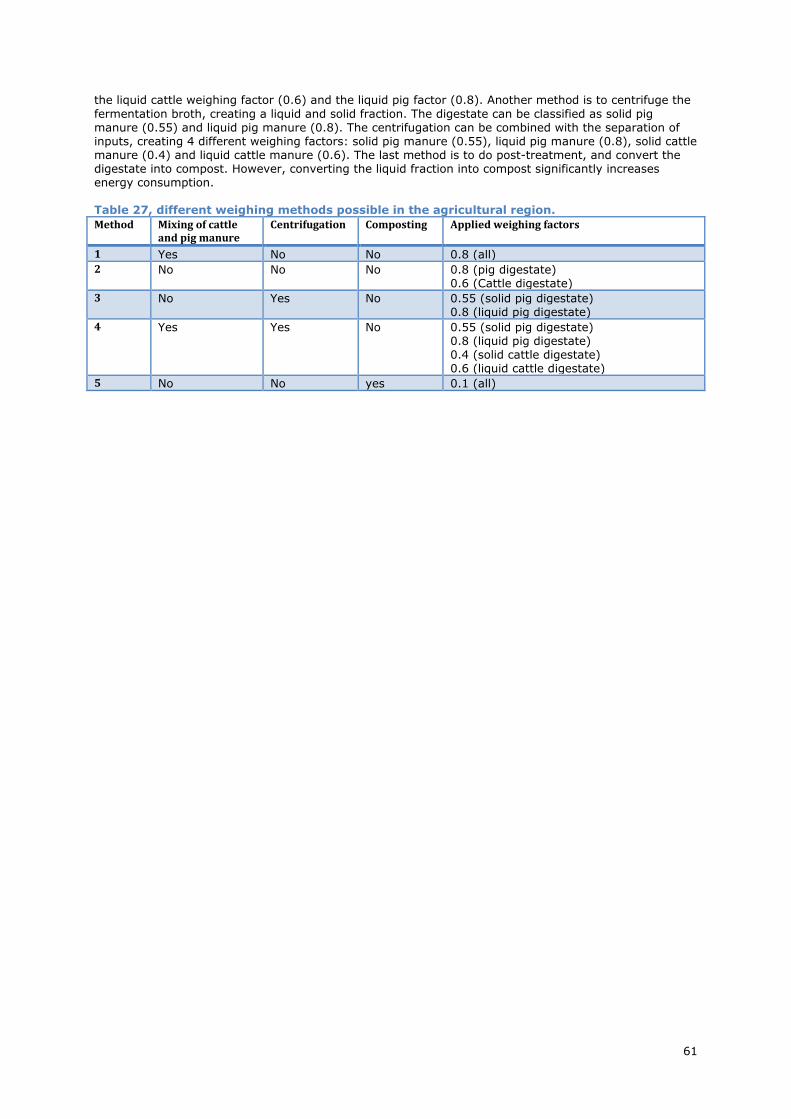
61

the liquid cattle weighing factor (0.6) and the liquid pig factor (0.8). Another method is to centrifuge the

fermentation broth, creating a liquid and solid fraction. The digestate can be classified as solid pig manure (0.55) and liquid pig manure (0.8). The centrifugation can be combined with the separation of inputs, creating 4 different weighing factors: solid pig manure (0.55), liquid pig manure (0.8), solid cattle manure (0.4) and liquid cattle manure (0.6). The last method is to do post-treatment, and convert the digestate into compost. However, converting the liquid fraction into compost significantly increases energy consumption.

Table 27, different weighing methods possible in the agricultural region.

Method Mixing of cattle and pig manure

Centrifugation Composting Applied weighing factors

1 Yes No No 0.8 (all)

2 No No No 0.8 (pig digestate) 0.6 (Cattle digestate)

3 No Yes No 0.55 (solid pig digestate) 0.8 (liquid pig digestate)

4 Yes Yes No 0.55 (solid pig digestate) 0.8 (liquid pig digestate) 0.4 (solid cattle digestate) 0.6 (liquid cattle digestate)

5 No No yes 0.1 (all)

62

Appendix V. Replacing imported feed with refined rapeseed Some optimisations were performed with refined rapeseed instead of imported soybean feed. The

composition of the refined rapeseed is given below:

Table 28, composition of refined rapeseed. (LEI 2013, Liu et al. 1994, Xu and diosady 2002, Mińkowski 2002)

Refined rapeseed

Dry matter 350 g/kg

Protein 850 g/kg DM

Sugars 60 g/kg DM

Lipids 2 g/kg DM

Fibres 1 g/kg DM

P 0 g/kg DM

K 0 g/kg DM

Cellulose 50 % of the fibres (assumed)

Hemicellulose 40 % of the fibres (assumed)

Lignin 10 % of the fibres (assumed)

The price of the refined rapeseed is estimated at 2200 euro per ton DM. Based on the composition of the refined rapeseed, the energy content is estimated at 12.3 GJ/ton DM for pigs and 11 GJ/ton DM for dairy cattle.

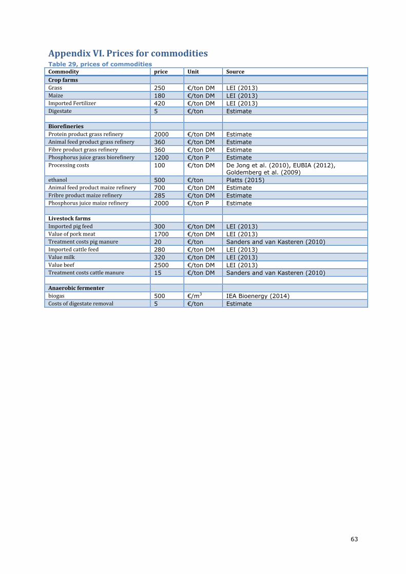
63

Appendix VI. Prices for commodities Table 29, prices of commodities

Commodity price Unit Source

Crop farms

Grass 250 €/ton DM LEI (2013)

Maize 180 €/ton DM LEI (2013)

Imported Fertilizer 420 €/ton DM LEI (2013)

Digestate 5 €/ton Estimate

Biorefineries

Protein product grass refinery 2000 €/ton DM Estimate

Animal feed product grass refinery 360 €/ton DM Estimate

Fibre product grass refinery 360 €/ton DM Estimate

Phosphorus juice grass biorefinery 1200 €/ton P Estimate

Processing costs 100 €/ton DM De Jong et al. (2010), EUBIA (2012), Goldemberg et al. (2009)

ethanol 500 €/ton Platts (2015)

Animal feed product maize refinery 700 €/ton DM Estimate

Fribre product maize refinery 285 €/ton DM Estimate

Phosphorus juice maize refinery 2000 €/ton P Estimate

Livestock farms

Imported pig feed 300 €/ton DM LEI (2013)

Value of pork meat 1700 €/ton DM LEI (2013)

Treatment costs pig manure 20 €/ton Sanders and van Kasteren (2010)

Imported cattle feed 280 €/ton DM LEI (2013)

Value milk 320 €/ton DM LEI (2013)

Value beef 2500 €/ton DM LEI (2013)

Treatment costs cattle manure 15 €/ton DM Sanders and van Kasteren (2010)

Anaerobic fermenter

biogas 500 €/m3 IEA Bioenergy (2014)

Costs of digestate removal 5 €/ton Estimate

64

Appendix VII. The mathematical model. Filename; ‘optniels2’ clear all

close all

clc

Jt=[];

Jbest=1000000; t=clock;

Tc=[];

while etime(clock,t) < 900

X_feed_cow = 32111; % 1 cow concentrates X_feed_pig = 05941; % 2 pig concentrates

% Artificial N, P and K for maize fields

X_Nasm=512; % 3

X_Pasm=324; % 4 X_Kasm=0; % 5

% Artificial N, P and K for grass fields

X_Nasg=867; % 6

X_Pasg=1; % 7

X_Kasg=1297; % 8

% Mais for biorefinery, cow and pig

X_maisb = 14223; X_maisc = 29950; X_maisp = 28770; % 9, 10, 11

% Grass for biorefinery and cow

X_grassb = 15738; X_grassc = 61354; % 12, 13

% Distribution parameters

% 14: byosense feed for cow. 15: grass for biorefinery grassa

p_bcow=.01; p_grassa=0.20; % 14 , 15

% 16: corn for byosense. 17: corn for cow. 18: corn for pig

p_byos=0.19; p_mcow=0.41; p_mpig=0.40; % 16,17,18 % Grassa High (19) and low (20) quality food for cow

p_cowH=0.01; p_cowL=0.01; %19,20

% Distrubtion of nutrients from fermenter to soil land

p_solsg=0.95; p_liqsg=0.55; % 21,22 fraction for gras land

% Distribution of fibre fraction over cattle and fermenter

p_fibrgcow=0.75; %fraction for cow

p_fibrbcow=0; %fraction for cow

% x0 = [X_feed_cow; X_feed_pig; X_Nasm; X_Pasm; X_Kasm;X_Nasg; X_Pasg; X_Kasg;...

% X_maisb; X_grassb]

x0 = [X_feed_cow; X_feed_pig; X_Nasm; X_Pasm; X_Kasm;X_Nasg; X_Pasg; X_Kasg;... X_maisb; X_maisc; X_maisp; X_grassb; X_grassc;...

p_bcow; p_grassa;p_byos; p_mcow; p_mpig; p_cowH; p_cowL;p_solsg;p_liqsg;p_fibrgcow];%

%for i=1:50

x0=x0+(x0.*rand(size(x0))-0.5);

%lower boundaries

xlb=[0; 0; 0; 0; 0; 0; 0; 0;...

0; 0; 0; 0; 0;... 0; 0; 0; 0; 0; 0; 0; 0; 0;0];

%upper boundaries

xub=[4.1e4; 3.1e4; 2e3; 2e3; 2e3; 3e3; 2e3; 2e3;... 1e5; 2e5; 1e5; 1e5; 2e5;...

1; 1; 1; 1; 1; 1; 1; 1; 1;1];

%% Compute zero of function

opt=optimset('Display','iter','TolFun',1e-6,'TolCon',1e-3);

[xopt,fopt] = fmincon(@niels,x0,[],[],[],[],xlb,xub,@nielsc,opt)

%% changes from initial

if fopt < Jbest

Jbest=fopt;

tc=etime(clock,t); Jt=[Jt;Jbest];

Tc=[Tc;tc];

y=[Jt Tc]

xbest=xopt; end

end

y

save('xbest.mat','xbest');

% end

Filename; ‘niels’

%optimization function

function [f]=niels(x)

[~,~,f]=nielsc(x);

Filename; ‘nielsc’ function [c,ceq,f]=nielsc(x)

% variable inputs. optimized in optjoep

X_feed_cow=x(1); X_feed_pig=x(2); % feed concentrates X_Nasm=x(3); X_Pasm=x(4); X_Kasm=x(5); % Artificial fertilizer for mais land

X_Nasg=x(6); X_Pasg=x(7); X_Kasg=x(8); % Artificial fertilizer for grass land

65

X_maisb=x(9); X_maisc=x(10); X_maisp=x(11); % Distribution of mais

X_grassb=x(12); X_grassc=x(13); % Distribution of grass

p_bcow=x(14); p_grassa=x(15); p_byos=x(16); p_mcow=x(17); p_mpig =x(18);

p_cowH=x(19); p_cowL=x(20);

p_solsg=x(21); p_liqsg=x(22);

p_fibrgcow=x(23);

p_fibrbcow=0;

%% Byosense

[X_protbf,X_sugbf,X_lipbf,X_fibrbf,X_Pbf,X_Kbf,X_celbf,X_hembf,X_ligbf... %byosense-fermentor

X_protbc,X_sugbc,X_lipbc,X_fibrbc,X_Pbc,X_Kbc,X_celbc,X_hembc,X_ligbc... %byosense-cow X_protbp,X_sugbp,X_lipbp,X_fibrbp,X_Pbp,X_Kbp,X_celbp,X_hembp,X_ligbp... %byosense-pig

X_protbsm,X_sugbsm,X_lipbsm,X_fibrbsm,X_Pbsm,X_Kbsm,X_celbsm,X_hembsm,X_ligbsm... %byosense-maisland

Y_eth,Y_eur_Byo,X_eur_BC,X_eur_BP]=Byosense(X_maisb,p_bcow,p_fibrbcow);

%% Grassa

[X_protgc,X_suggc,X_lipgc,X_fibrgc,X_Pgc,X_Kgc,X_celgc,X_hemgc,X_liggc,... %Grassa-cow

X_protgp,X_suggp,X_lipgp,X_fibrgp,X_Pgp,X_Kgp,X_celgp,X_hemgp,X_liggp,... %Grassa-pig

X_protgf,X_suggf,X_lipgf,X_fibrgf,X_Pgf,X_Kgf,X_celgf,X_hemgf,X_liggf,... %Grassa-fermentor

X_protgsg,X_suggsg,X_lipgsg,X_fibrgsg,X_Pgsg,X_Kgsg,X_celgsm,X_hemgsm,X_liggsm... %Grassa-grassland ,Y_eur_GA,X_eur_GC,X_eur_GP]=GRASSA(X_grassb,p_cowH,p_cowL,p_fibrgcow);

%% Cow

[X_Ncf,X_Pcf,X_POc,X_Kcf,X_cow,X_celcf,X_hemcf,X_ligcf,Y_Nmeat,Y_Pmeat,Y_Kmeat,... Y_Nmilk,Y_Pmilk,Y_Kmilk,Y_En_Cow,Y_eur_Cow,X_protc]=Cow...

(X_feed_cow,X_maisc,X_grassc,...% concentrates & roughage

X_eur_GC,X_protgc,X_suggc,X_lipgc,X_fibrgc,X_Pgc,X_Kgc,X_celgc,X_hemgc,X_liggc,... % Grassa-cow

X_eur_BC,X_protbc,X_sugbc,X_lipbc,X_fibrbc,X_Pbc,X_Kbc,X_celbc,X_hembc,X_ligbc); % Byosense-cow

%% Pig

[X_Npf,X_Ppf,X_POp,X_Kpf,X_pig,X_celpf,X_hempf,X_ligpf,Y_meat,Y_Npmeat,Y_Ppmeat,Y_Kpmeat,...

Y_En_Pig,Y_eur_Pig,X_protp]=Pig(X_maisp,X_feed_pig,... X_eur_GP,X_protgp,X_suggp,X_lipgp,X_fibrgp,X_Pgp,X_Kgp,X_celgp,X_hemgp,X_liggp,... %Grassa-pig

X_eur_BP,X_protbp,X_sugbp,X_lipbp,X_fibrbp,X_Pbp,X_Kbp,X_celbp,X_hembp,X_ligbp); %Byosense-pig

%% Fermentor

[X_Nfsm,X_Pfsm,X_Kfsm,X_Dism,X_celfsm,X_hemfsm,X_ligfsm... ,X_Nfsg,X_Pfsg,X_Kfsg,X_Disg,X_celfsg,X_hemfsg,X_ligfsg,Y_Wmet,Y_eur_BG,Y_fibrex,...

Y_H2Sbg,X_mod,Vp_H2S,X_Sin,X_Sef]...

=Fermentor(X_pig,X_Npf,X_Ppf,X_Kpf,X_celpf,X_hempf,X_ligpf,...

X_cow,X_Ncf,X_Pcf,X_Kcf,X_celcf,X_hemcf,X_ligcf,... X_protbf,X_sugbf,X_lipbf,X_fibrbf,X_Pbf,X_Kbf,X_celbf,X_hembf,X_ligbf,... % Byosense-fermentor

X_protgf,X_suggf,X_lipgf,X_fibrgf,X_Pgf,X_Kgf,X_celgf,X_hemgf,X_liggf,p_solsg,p_liqsg);

%% Soilgrass [X_Nsgg,X_Psgg,X_Ksgg,X_Nlsgtot,N_suplg,P_suplg,K_suplg,Y_Pgloss,Y_Kgloss,X_AFgtot,...

Y_grassa,Y_grascow,Y_HAg,Y_eur_Gr,A_digg,A_Ng,A_Pg,A_Kg] = Soilgrass...

(X_Nfsg,X_Pfsg,X_Kfsg,X_Disg,X_celfsg,X_hemfsg,X_ligfsg,X_Nasg,X_Pasg,X_Kasg,X_protgsg,X_Pgsg,X_Kgsg,p_grassa);

%% Soilmaize [X_Nsmm,X_Psmm,X_Ksmm,X_Nlmgtot,N_suplm,P_suplm,K_suplm,Y_Pmloss,Y_Kmloss,X_AFmtot,...

Y_Maisb,Y_Maisc,Y_Maisp,Y_HAm,Y_eur_Ma,A_digm,A_Nm,A_Pm,A_Km] = Soilmaize...

(X_Nfsm,X_Pfsm,X_Kfsm,X_Dism,X_celfsm,X_hemfsm,X_ligfsm,X_Nasm,X_Pasm,X_Kasm,X_protbsm,X_Pbsm,X_Kbsm,...

p_byos,p_mcow,p_mpig);

ceq=[1e-3; 1e-3; 1e-3; 1e-3; 1e-3; 1e-4; 1e-4; 1e-3 ;1e-2; 1].*...

([X_maisb; X_maisc; X_maisp; X_grassb; X_grassc; Y_En_Cow; Y_En_Pig;... X_protc;X_protp;p_byos+p_mcow+p_mpig]-...

[Y_Maisb; Y_Maisc; Y_Maisp; Y_grassa; Y_grascow; 8.7e5; 5e5; 2.2e4; 6e3;1]);

c=[Y_HAg+Y_HAm-12000];

f=-1e-07*(Y_eur_Gr+Y_eur_BG+Y_eur_Byo+Y_eur_Cow+Y_eur_GA+Y_eur_Ma+Y_eur_Pig)+1e-07*1000*(X_Pcf+X_Ppf);

Filename; ‘Byosens’

% function on the byosense fermentor

function [Y_protbf,Y_sugbf,Y_lipbf,Y_fibrbf,Y_Pbf,Y_Kbf,Y_celbf,Y_hembf,Y_ligbf... %byosense-fermentor

Y_protbc,Y_sugbc,Y_lipbc,Y_fibrbc,Y_Pbc,Y_Kbc,Y_celbc,Y_hembc,Y_ligbc... %byosense-cow

Y_protbp,Y_sugbp,Y_lipbp,Y_fibrbp,Y_Pbp,Y_Kbp,Y_celbp,Y_hembp,Y_ligbp... %byosense-pig Y_protbsm,Y_sugbsm,Y_lipbsm,Y_fibrbsm,Y_Pbsm,Y_Kbsm,Y_celbsm,Y_hembsm,Y_ligbsm... %byosense-mais

Y_eth,Y_eur_Byo,Y_eur_BC,Y_eur_BP]=Byosense(X_mais,p_bcow,p_fibrbcow)

% Pre-treatment

%% Input (1): % X_mais = maize/corn [ton/year]

%

%% Corn is refined into 4 fractions/streams:

% 1 Corn stalks (fibres for biogas)

% 2 Animal Feed % 3 Ethanol 60%

% 4 Corn juice

%

% Stream 1 consists mainly of fibres and is separated from the cobs to % use as substrate in biogas fementor

% After separation the cobs are fermented and that broth is centrifuged.

% Stream 2, the pellet, consisting of protein, sugar, lipids, fibres, potassium

% and phoshorous is fed to cows and pigs (ratio p_bcow : 1-p_bcow) % Stream 3 is obtained by distilling the liquid phase after centrifugation

% a 60% ethanol 40% water mixture is produced.

% Stream 4 is the distilled waste, which contains nutrients that can go

% back to the corn land %

% summarizing there are 4 output streams going to 5 different targets:

66

% Stream 1 to biogas (bf)

% Stream 2 to cows (bc) and pigs (bp)

% Stream 3 to customers, Y_eth

% Stream 4 to maize/corn field (bm) %

% Output (6):

% outputs for fermentor (bf): stream 1

% Y_protbf = outcoming protein to Fermentor [ton/year]

% Y_sugbf = outcoming sugars to Fermentor [ton/year] % Y_lipbf = outcoming lipids to Fermentor [ton/year]

% Y_fibrbf = outcoming fibres to Fermentor [ton/year]

% Y_Pbf = outcoming phosphorous for Fermentor [ton/year]

% Y_Kbf = outcoming potassium for Fermentor [ton/year] %

% outputs for cows (bc): stream 2

% Y_protbc = outcoming protein for cowfeed [ton/year]

% Y_sugbc = outcoming sugars for cow [ton/year] % Y_lipbc = outcoming lipids for cow [ton/year]

% Y_fibrbc = outcoming fibres for cow [ton/year]

% Y_Pbc = outcoming phosphorous in feed cow [ton/year]

% Y_Kbc = outcoming potassium in feed cow [ton/year]

% % outputs for Pig (bp): stream 2

% Y_protbp = outcoming protein for pigfeed [ton/year]

% Y_sugbp = outcoming sugars for pig [ton/year]

% Y_lipbp = outcoming lipids for pig [ton/year] % Y_fibrbp = outcoming fibres for pig [ton/year]

% Y_Pbp = outcoming phosphorous in feed pig [ton/year]

% Y_Kbp = outcoming potassium in feed pig [ton/year]

% % outputs for ethanol : stream 3

% Y_eth = produced ethanol (not water) [ton/year]

% Stream 4 recycling to maize land (bm): stream 4

% Y_protbm = outcoming protein to corn land [ton/year] % Y_sugbm = outcoming sugars to corn land [ton/year]

% Y_lipbm = outcoming lipids to corn land [ton/year]

% Y_fibrbm = outcoming fibres to corn land [ton/year]

% Y_Pbm = outcoming phosphorous for corn land [ton/year]

% Y_Kbm = outcoming potassium for corn land [ton/year] % Y_eur_Byo= Profit of Byosense refinery [€/year]

% Y_eur_BC = Value of animal feed stream, cow [€/year]

% Y_eur_BP = Value of animal feed stream, pig [€/year]

%scenario

%p_bcow=1;

%% composition of dry corn p_pro=0.0625; % [kg/kg] protein per kg of dry mais

p_sug=0.39; % [kg/kg] sugar per kg of dry mais

p_lip=0.04; % [kg/kg] lipid per kg of dry mais

p_eth=0.15; % [kg/kg] ethanol per kg of dry mais

p_fibr=0.38; % [kg/kg] fibres per kg of dry mais p_P=0.0019; % [kg/kg] phosphorous per kg of dry mais

p_K=0.010; % [kg/kg] potassium per kg of dry mais

p_cel=0.200; % amount of cellulose [kg/kg DM]

p_hem=0.150; % amount of hemicellulose [kg/kg DM] p_lig=0.030; % amount of lignin [kg/kg DM]

p_ethrec=0.95; % ethanol recovery

%% Fractions of the compound that end up in the fibre output (fermentor): p_protbf=0; % protein fraction ending up in fibre output

p_sugbf=0; % sugar fraction ending up in fibre output

p_lipbf=0; % lipid fraction ending up in fibre output

p_fibrbf=1; % Fibre fraction ending up in fibre output p_Pbf=0.378; % Phosphorous fraction ending up in fibre output

p_Kbf=0.380; % Potassium fraction ending up in fibre output

%% Fermentor (bf)

Y_protbf=p_pro*p_protbf*X_mais*(1-p_fibrbcow); Y_sugbf=p_sug*p_sugbf*X_mais*(1-p_fibrbcow);

Y_lipbf=p_lip*p_lipbf*X_mais*(1-p_fibrbcow);

Y_fibrbf=p_fibr*p_fibrbf*X_mais*(1-p_fibrbcow);

Y_Pbf=p_P*p_Pbf*X_mais*(1-p_fibrbcow); Y_Kbf=p_K*p_Kbf*X_mais*(1-p_fibrbcow);

Y_celbf=p_fibrbf*p_cel*X_mais*(1-p_fibrbcow);

Y_hembf=p_fibrbf*p_hem*X_mais*(1-p_fibrbcow);

Y_ligbf=p_fibrbf*p_lig*X_mais*(1-p_fibrbcow); X_stream1=Y_protbf+Y_sugbf+Y_lipbf+Y_fibrbf+Y_Pbf+Y_Kbf;

%% Fractions of the compound that end up in the Animal Feed (AF) output:

p_protAF=0.9; % protein fraction ending up in feed output

p_sugAF=0.208; % sugar fraction ending up in feed output p_lipAF=0.9; % lipid fraction ending up in feed output

p_fibrAF=0; % feed fraction ending up in feed output

p_PAF=0.099; % Phosphorous fraction ending up in feed output

p_KAF=0.099; % Potassium fraction ending up in feed output

%% Animal Feed

X_prot=p_pro*p_protAF*X_mais;

X_sug=p_sug*p_sugAF*X_mais; X_lip=p_lip*p_lipAF*X_mais;

X_fibr=p_fibr*p_fibrAF*X_mais;

X_P=p_P*p_PAF*X_mais;

X_K=p_K*p_KAF*X_mais; Y_cel=p_fibrAF*p_cel*X_mais;

Y_hem=p_fibrAF*p_hem*X_mais;

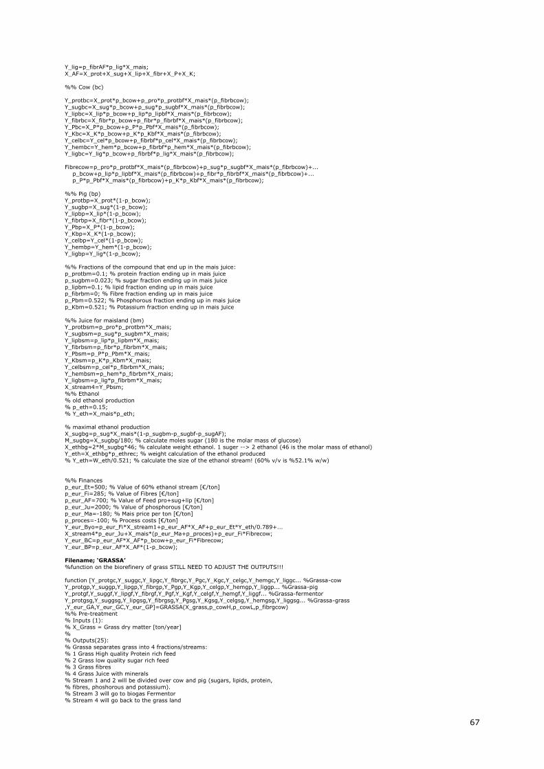
67

Y_lig=p_fibrAF*p_lig*X_mais;

X_AF=X_prot+X_sug+X_lip+X_fibr+X_P+X_K;

%% Cow (bc)

Y_protbc=X_prot*p_bcow+p_pro*p_protbf*X_mais*(p_fibrbcow);

Y_sugbc=X_sug*p_bcow+p_sug*p_sugbf*X_mais*(p_fibrbcow);

Y_lipbc=X_lip*p_bcow+p_lip*p_lipbf*X_mais*(p_fibrbcow);

Y_fibrbc=X_fibr*p_bcow+p_fibr*p_fibrbf*X_mais*(p_fibrbcow); Y_Pbc=X_P*p_bcow+p_P*p_Pbf*X_mais*(p_fibrbcow);

Y_Kbc=X_K*p_bcow+p_K*p_Kbf*X_mais*(p_fibrbcow);

Y_celbc=Y_cel*p_bcow+p_fibrbf*p_cel*X_mais*(p_fibrbcow);

Y_hembc=Y_hem*p_bcow+p_fibrbf*p_hem*X_mais*(p_fibrbcow); Y_ligbc=Y_lig*p_bcow+p_fibrbf*p_lig*X_mais*(p_fibrbcow);

Fibrecow=p_pro*p_protbf*X_mais*(p_fibrbcow)+p_sug*p_sugbf*X_mais*(p_fibrbcow)+...

p_bcow+p_lip*p_lipbf*X_mais*(p_fibrbcow)+p_fibr*p_fibrbf*X_mais*(p_fibrbcow)+... p_P*p_Pbf*X_mais*(p_fibrbcow)+p_K*p_Kbf*X_mais*(p_fibrbcow);

%% Pig (bp)

Y_protbp=X_prot*(1-p_bcow);

Y_sugbp=X_sug*(1-p_bcow); Y_lipbp=X_lip*(1-p_bcow);

Y_fibrbp=X_fibr*(1-p_bcow);

Y_Pbp=X_P*(1-p_bcow);

Y_Kbp=X_K*(1-p_bcow); Y_celbp=Y_cel*(1-p_bcow);

Y_hembp=Y_hem*(1-p_bcow);

Y_ligbp=Y_lig*(1-p_bcow);

%% Fractions of the compound that end up in the mais juice:

p_protbm=0.1; % protein fraction ending up in mais juice

p_sugbm=0.023; % sugar fraction ending up in mais juice

p_lipbm=0.1; % lipid fraction ending up in mais juice p_fibrbm=0; % Fibre fraction ending up in mais juice

p_Pbm=0.522; % Phosphorous fraction ending up in mais juice

p_Kbm=0.521; % Potassium fraction ending up in mais juice

%% Juice for maisland (bm) Y_protbsm=p_pro*p_protbm*X_mais;

Y_sugbsm=p_sug*p_sugbm*X_mais;

Y_lipbsm=p_lip*p_lipbm*X_mais;

Y_fibrbsm=p_fibr*p_fibrbm*X_mais; Y_Pbsm=p_P*p_Pbm*X_mais;

Y_Kbsm=p_K*p_Kbm*X_mais;

Y_celbsm=p_cel*p_fibrbm*X_mais;

Y_hembsm=p_hem*p_fibrbm*X_mais; Y_ligbsm=p_lig*p_fibrbm*X_mais;

X_stream4=Y_Pbsm;

%% Ethanol

% old ethanol production

% p_eth=0.15; % Y_eth=X_mais*p_eth;

% maximal ethanol production

X_sugbg=p_sug*X_mais*(1-p_sugbm-p_sugbf-p_sugAF); M_sugbg=X_sugbg/180; % calculate moles sugar (180 is the molar mass of glucose)

X_ethbg=2*M_sugbg*46; % calculate weight ethanol. 1 suger --> 2 ethanol (46 is the molar mass of ethanol)

Y_eth=X_ethbg*p_ethrec; % weight calculation of the ethanol produced

% Y_eth=W_eth/0.521; % calculate the size of the ethanol stream! (60% v/v is %52.1% w/w)

%% Finances

p_eur_Et=500; % Value of 60% ethanol stream [€/ton] p_eur_Fi=285; % Value of Fibres [€/ton]

p_eur_AF=700; % Value of Feed pro+sug+lip [€/ton]

p_eur_Ju=2000; % Value of phosphorous [€/ton]

p_eur_Ma=-180; % Mais price per ton [€/ton]

p_proces=-100; % Process costs [€/ton] Y_eur_Byo=p_eur_Fi*X_stream1+p_eur_AF*X_AF+p_eur_Et*Y_eth/0.789+...

X_stream4*p_eur_Ju+X_mais*(p_eur_Ma+p_proces)+p_eur_Fi*Fibrecow;

Y_eur_BC=p_eur_AF*X_AF*p_bcow+p_eur_Fi*Fibrecow;

Y_eur_BP=p_eur_AF*X_AF*(1-p_bcow);

Filename; ‘GRASSA’

%function on the biorefinery of grass STILL NEED TO ADJUST THE OUTPUTS!!!

function [Y_protgc,Y_suggc,Y_lipgc,Y_fibrgc,Y_Pgc,Y_Kgc,Y_celgc,Y_hemgc,Y_liggc... %Grassa-cow

Y_protgp,Y_suggp,Y_lipgp,Y_fibrgp,Y_Pgp,Y_Kgp,Y_celgp,Y_hemgp,Y_liggp... %Grassa-pig

Y_protgf,Y_suggf,Y_lipgf,Y_fibrgf,Y_Pgf,Y_Kgf,Y_celgf,Y_hemgf,Y_liggf... %Grassa-fermentor

Y_protgsg,Y_suggsg,Y_lipgsg,Y_fibrgsg,Y_Pgsg,Y_Kgsg,Y_celgsg,Y_hemgsg,Y_liggsg... %Grassa-grass

,Y_eur_GA,Y_eur_GC,Y_eur_GP]=GRASSA(X_grass,p_cowH,p_cowL,p_fibrgcow) %% Pre-treatment

% Inputs (1):

% X_Grass = Grass dry matter [ton/year]

% % Outputs(25):

% Grassa separates grass into 4 fractions/streams:

% 1 Grass High quality Protein rich feed

% 2 Grass low quality sugar rich feed % 3 Grass fibres

% 4 Grass Juice with minerals

% Stream 1 and 2 will be divided over cow and pig (sugars, lipids, protein,

% fibres, phoshorous and potassium). % Stream 3 will go to biogas Fermentor

% Stream 4 will go back to the grass land

68

%

% outputs for cow (gc):

% Y_protgc = outcoming protein for cowfeed [ton/year]

% Y_suggc = outcoming sugars for cow [ton/year] % Y_lipgc = outcoming lipids for cow [ton/year]

% Y_fibrgc = outcoming fibres for cow [ton/year]

% Y_Pgc = outcoming phosphorous in feed cow [ton/year]

% Y_Kgc = outcoming potassium in feed cow [ton/year]

% % outputs for Pig (gp):

% Y_protgp = outcoming protein for pigfeed [ton/year]

% Y_suggp = outcoming sugars for pig [ton/year]

% Y_lipgp = outcoming lipids for pig [ton/year] % Y_fibrgp = outcoming fibres for pig [ton/year]

% Y_Pgp = outcoming phosphorous in feed pig [ton/year]

% Y_Kgp = outcoming potassium in feed pig [ton/year]

% % outputs for Fermentor (gf):

% Y_protgf = outcoming protein to Fermentor [ton/year]

% Y_suggf = outcoming sugars to Fermentor [ton/year]

% Y_lipgf = outcoming lipids to Fermentor [ton/year]

% Y_fibrgf = outcoming fibres to Fermentor [ton/year] % Y_Pgf = outcoming phosphorous for Fermentor [ton/year]

% Y_Kgf = outcoming potassium for Fermentor [ton/year]

%

% Stream 4 recycling to grass land (gg) % Y_protgg = outcoming protein to grass land [ton/year]

% Y_suggg = outcoming sugars to grass land [ton/year]

% Y_lipgg = outcoming lipids to grass land [ton/year]

% Y_fibrgg = outcoming fibres to grass land [ton/year] % Y_Pgg = outcoming phosphorous for grass land [ton/year]

% Y_Kgg = outcoming potassium for grass land [ton/year]

%

% Y_eur_GA = Profit of GRASSA unit [€/year] % Y_eur_GC = Value of cow feed stream 1&2 [€/year]

% Y_eur_GP = Value of pig feed stream 1&2 [€/year]

%scenario parameters

%p_cowH=1; %p_cowL=1;

%% Composition of dry grass

p_pro=0.21; % kg protein per kg of dry grass p_sug=0.18; % kg sugar per kg of dry grass

p_lip=0.04; % fraction of lipids in the dry grass [kg/kg]

p_fibr=0.5; % fraction of fibres in the dry grass [kg/kg]

p_P=0.0035; % fraction of phosphorous in the dry grass[kg/kg] p_K=0.025; % fraction of potassium in the dry grass[kg/kg]

% fraction of fibres

p_cel=0.250; % cellulose fraction of DM [kg/kg]

p_hem=0.225; % Hemicellulose fraction of DM [kg/kg]

p_lig=0.025; % Lignin fraction of DM [kg/kg] % First separation into grass fibres and juice.

% p_fibrcow=1;

%% Fractions of the compound that end up in the fibre output: p_protgf=0.33; % protein fraction ending up in fibre output

p_suggf=0.25; % sugar fraction ending up in fibre output

p_lipgf=0.1; % lipid fraction ending up in fibre output

p_fibrgf=0.84; % Fibre fraction ending up in fibre output p_Pgf=0.5; % Phosphorous fraction ending up in fibre output

p_Kgf=0.209; % Potassium fraction ending up in fibre output

% Juice is separated again into high (H) and low (L) quality feed and juice.

%% Fractions of the compound that end up in the High quality feed:

p_protgH=0.67; % protein fraction ending up in High quality feed

p_suggH=0.1875; % sugar fraction ending up in High quality feed

p_lipgH=0.81; % lipid fraction ending up in High quality feed p_fibrgH=0.16; % Fibre fraction ending up in High quality feed

p_PgH=0.125; % Phosphorous fraction ending up in High quality feed

p_KgH=0.185; % Potassium fraction ending up in High quality feed

X_protgH=p_pro*p_protgH*X_grass;

X_suggH=p_sug*p_suggH*X_grass;

X_lipgH=p_lip*p_lipgH*X_grass;

X_fibrgH=p_fibr*p_fibrgH*X_grass; X_PgH=p_P*p_PgH*X_grass;

X_KgH=p_K*p_KgH*X_grass;

X_celgH=p_fibrgH*p_cel*X_grass;

X_hemgH=p_fibrgH*p_hem*X_grass;

X_liggH=p_fibrgH*p_lig*X_grass; X_stream1=(X_protgH+X_suggH+X_lipgH+X_fibrgH+X_PgH+X_KgH);

%% Fractions of the compound that end up in the Low quality feed:

p_protgL=0.0; % protein fraction ending up in Low quality feed p_suggL=0.45; % sugar fraction ending up in Low quality feed

p_lipgL=0.09; % lipid fraction ending up in Low quality feed

p_fibrgL=0; % Fibre fraction ending up in Low quality feed

p_PgL=0.1875; % Phosphorous fraction ending up in Low quality feed p_KgL=0.121; % Potassium fraction ending up in Low quality feed

X_protgL=p_pro*p_protgL*X_grass;

X_suggL=p_sug*p_suggL*X_grass; X_lipgL=p_lip*p_lipgL*X_grass;

X_fibrgL=p_fibr*p_fibrgL*X_grass;

69

X_PgL=p_P*p_PgL*X_grass;

X_KgL=p_K*p_KgL*X_grass;

X_celgL=p_fibrgL*p_cel*X_grass;

X_hemgL=p_fibrgL*p_hem*X_grass; X_liggL=p_fibrgL*p_lig*X_grass;

X_stream2=X_protgL+X_suggL+X_lipgL+X_fibrgL+X_PgL+X_KgL;

% Final leftover is the grass juice which takes up the rest of the

% nutrients and is spread onto the grass land.

%% Fractions of the compound that end up in the Grass juice:

p_protgg=0.00; % protein fraction ending up in Grass juice

p_suggg=0.1125; % sugar fraction ending up in Grass juice p_lipgg=0.0; % lipid fraction ending up in Grass juice

p_fibrgg=0; % Fibre fraction ending up in Grass juice

p_Pgg=0.1875; % Phosphorous fraction ending up in Grass juice

p_Kgg=0.485; % Potassium fraction ending up in Grass juice

% %% Cow new distribution

% Y_protgc=X_protgL*p_cowL+X_protgH*p_cowH;

% Y_suggc=X_suggL*p_cowL+X_suggH*p_cowH;

% Y_lipgc=X_lipgL*p_cowL+X_lipgH*p_cowH; % Y_fibrgc=X_fibrgL*p_cowL+X_fibrgH*p_cowH;

% Y_Pgc=X_PgL*p_cowL+X_PgH*p_cowH;

% Y_Kgc=X_KgL*p_cowL+X_KgH*p_cowH;

% Y_celgc=X_celgH*p_cowH+X_celgL*p_cowL; % Y_hemgc=X_hemgH*p_cowH+X_hemgL*p_cowL;

% Y_liggc=X_liggH*p_cowH+X_liggL*p_cowL;

%% Pig Y_protgp=X_protgL*(1-p_cowL)+X_protgH*(1-p_cowH);

Y_suggp=X_suggL*(1-p_cowL)+X_suggH*(1-p_cowH);

Y_lipgp=X_lipgL*(1-p_cowL)+X_lipgH*(1-p_cowH);

Y_fibrgp=X_fibrgL*(1-p_cowL)+X_fibrgH*(1-p_cowH); Y_Pgp=X_PgL*(1-p_cowL)+X_PgH*(1-p_cowH);

Y_Kgp=X_KgL*(1-p_cowL)+X_KgH*(1-p_cowH);

Y_celgp=X_celgL*(1-p_cowL)+X_celgH*(1-p_cowH);

Y_hemgp=X_hemgL*(1-p_cowL)+X_hemgH*(1-p_cowH);

Y_liggp=X_liggL*(1-p_cowL)+X_liggH*(1-p_cowH);

%% Fermentor

Y_protfs=p_pro*p_protgf*X_grass;

Y_sugfs=p_sug*p_suggf*X_grass; Y_lipfs=p_lip*p_lipgf*X_grass;

Y_fibrfs=p_fibr*p_fibrgf*X_grass;

Y_Pfs=p_P*p_Pgf*X_grass;

Y_Kfs=p_K*p_Kgf*X_grass; Y_celfs=p_fibrgf*p_cel*X_grass;

Y_hemfs=p_fibrgf*p_hem*X_grass;

Y_ligfs=p_fibrgf*p_lig*X_grass;

X_stream3=Y_protfs+Y_sugfs+Y_lipfs+Y_fibrfs+Y_Pfs+Y_Kfs;

%% Cow

Y_protgc=X_protgL*p_cowL+X_protgH*p_cowH+(Y_protfs*p_fibrgcow);

Y_suggc=X_suggL*p_cowL+X_suggH*p_cowH+Y_sugfs*p_fibrgcow;

Y_lipgc=X_lipgL*p_cowL+X_lipgH*p_cowH+Y_lipfs*p_fibrgcow; Y_fibrgc=X_fibrgL*p_cowL+X_fibrgH*p_cowH+Y_fibrfs*p_fibrgcow;

Y_Pgc=X_PgL*p_cowL+X_PgH*p_cowH+Y_Pfs*p_fibrgcow;

Y_Kgc=X_KgL*p_cowL+X_KgH*p_cowH+Y_Kfs*p_fibrgcow;

Y_celgc=X_celgH*p_cowH+X_celgL*p_cowL+Y_celfs*p_fibrgcow; Y_hemgc=X_hemgH*p_cowH+X_hemgL*p_cowL+Y_hemfs*p_fibrgcow;

Y_liggc=X_liggH*p_cowH+X_liggL*p_cowL+Y_ligfs*p_fibrgcow;

Y_protgf=Y_protfs*(1-p_fibrgcow); Y_suggf=Y_sugfs*(1-p_fibrgcow);

Y_lipgf=Y_lipfs*(1-p_fibrgcow);

Y_fibrgf=Y_fibrfs*(1-p_fibrgcow);

Y_Pgf=Y_Pfs*(1-p_fibrgcow);

Y_Kgf=Y_Kfs*(1-p_fibrgcow); Y_celgf=Y_celfs*(1-p_fibrgcow);

Y_hemgf=Y_hemfs*(1-p_fibrgcow);

Y_liggf=Y_ligfs*(1-p_fibrgcow);

%% Grassland

Y_protgsg=p_pro*p_protgg*X_grass; Y_suggsg=p_sug*p_suggg*X_grass;

Y_lipgsg=p_lip*p_lipgg*X_grass;

Y_fibrgsg=p_fibr*p_fibrgg*X_grass;

Y_Pgsg=p_P*p_Pgg*X_grass;

Y_Kgsg=p_K*p_Kgg*X_grass; X_stream4=Y_Pgsg;

Y_celgsg=p_fibrgg*p_cel*X_grass;

Y_hemgsg=p_fibrgg*p_hem*X_grass;

Y_liggsg=p_fibrgg*p_lig*X_grass;

%% Finances

p_eur_FH= 2000; % Value of High quality feed (stream1) [€/ton]

p_eur_FL= 360; % Value of Low quality feed (stream2) [€/ton] p_eur_Fi= 360; % Value of Fibres stream 3 [€/ton]

p_eur_Ju=1200; % Value of phosphorous [€/ton]

p_eur_Gr= -250; % grass value per ton (input=costs) [€/ton]

p_proces=-100; % Process costs [€/ton]

Y_eur_GA=p_eur_FH*X_stream1+p_eur_FL*X_stream2+p_eur_Fi*X_stream3...

70

+p_eur_Ju*X_stream4+X_grass*(p_eur_Gr+p_proces);

Y_eur_GC=p_eur_FH*X_stream1*p_cowH+p_eur_FL*X_stream2*p_cowL+X_stream3*p_fibrgcow*p_eur_Fi;

Y_eur_GP=p_eur_FH*X_stream1*(1-p_cowH)+p_eur_FL*X_stream2*(1-p_cowL);

Filename; ‘Cow’

% function for cowfarmers

function [Y_Ncf,Y_Pcf,Y_POc,Y_Kcf,Y_man,Y_celcf,Y_hemcf,Y_ligcf,Y_Nmeat,Y_Pmeat,Y_Kmeat,...

Y_Nmilk,Y_Pmilk,Y_Kmilk,Y_En_Cow,Y_eur_Cow,X_protc]=Cow... (X_feed_cow,X_mais,X_grassc,...% concentrates & roughage

X_eur_GC,X_protgc,X_suggc,X_lipgc,X_fibrgc,X_Pgc,X_Kgc,X_celgc,X_hemgc,X_liggc,... % Grassa-cow

X_eur_BC,X_protbc,X_sugbc,X_lipbc,X_fibrbc,X_Pbc,X_Kbc,X_celbc,X_hembc,X_ligbc) % Byosense-cow

%% Information %Cow:% 20,000 Cows require 140,000 ton of feed whereof 22,000 ton protein

%

% Inputs (17):

% X_feed = Cow feed (20% protein) [ton/year] % X_mais = unrefined mais feed [ton/year]

% X_grass = unrefined grass feed [ton/year]

%

% refined feed from byosense (corn):

% X_protbc = refined corn protein for cow [ton/year] % X_sugbc = refined corn sugars for cow [ton/year]

% X_lipbc = refined corn lipids for cow [ton/year]

% X_fibrbc = refined corn fibres for cow [ton/year]

% X_Pbc = phosphorous in refined corn cow feed [ton/year] % X_Kbc = potassium in refined corn cow feed [ton/year]

% X_eur_BC = Value of refined corn cow feed [€/year]

%

% refined feed from grassa (grass) % X_protgc = refined grass protein for cow [ton/year]

% X_suggc = refined grass sugars for cow [ton/year]

% X_lipgc = refined grass lipids for cow [ton/year]

% X_fibrgc = refined grass fibres for cow [ton/year] % X_Pgc = phosphorous in refined grass cow feed [ton/year]

% X_Kgc = potassium in refined grass cow feed [ton/year]

% X_eur_GC = Value of refined grass cow feed [€/year]

%

% constraint: % X_protm+X_protg+p_feed*X_feed+X_grass*p_feed+X_mais*0.08=22,000 ton

%

% Outputs (12):

% Y_man = Manure produced [m3/year] % Manure, containing N, P and K, goes from Cow to fermentor. Abr: cf

% Y_Ncf = Nitrogen produced [ton/year]

% Y_Pcf = Phosphorous produced [ton/year]

% Y_Kcf = Potassium produced [ton/year] %

% The Cow produces milk with N, P and K. Abr: milk

% Y_Nmilk = Nitrogen produced [ton/year]

% Y_Pmilk = Phosphorous produced [ton/year]

% Y_Kmilk = Potassium produced [ton/year] %

% The Cow accumulates N, P and K in its muscles (meat) Abr: meat

% Y_Nmeat = Nitrogen produced [ton/year]

% Y_Pmeat = Phosphorous produced [ton/year] % Y_Kmeat = Potassium produced [ton/year]

%

% Energy output for cow

% Y_En_Cow = Energy present in cowfeed [GJ/year] %

% Costs & profit

% Y_eur_Cow= Profit of Cow Farm [€/year]

%% parameters, characteristics of the Cow

p_milk= 1.20; % kg milk produced per kg food

p_N= 1/6.25; % kg N per kg protein (all protein)

p_manc= 2.3; % m3 manure produced per ton food (prot+sug)

p_meatc= 1/40; % 0.0082 kg meat produced per kg food. Assumed 20 kg dm % uptake per day and lifetime of 5 year with 300 kg meat.

p_dryc=0.1; %ton dry matter per m3 cow manure (assume density 1000kg/m3)

p_meat=0.5; % meat fraction on Slaughtered Cattle

% Corn properties

p_protm=0.0625; % kg protein per kg dry matter of unrefined mais

p_sugm= 0.39; % kg sugar per kg dry matter of unrefined mais

p_lipm=0.04; % kg lipid per kg dry matter of unrefined mais p_fibrm=0.38; % kg fibre per kg dry matter of unrefined mais

p_Pm= 0.0019; % kg P per kg dry matter of unrefined mais

p_Km= 0.010; % kg K per kg dry matter of unrefined mais

p_celm=0.200; % amount of cellulose [kg/kg DM]

p_hemm=0.150; % amount of hemicellulose [kg/kg DM] p_ligm=0.030; % amount of lignin [kg/kg DM]

% Composition of dry grass

p_protg=0.21; % kg protein per kg of dry grass p_sugg=0.2; % kg sugar per kg of dry grass

p_lipg=0.04; % fraction of lipids in the dry grass [kg/kg]

p_fibrg=0.5; % fraction of fibres in the dry grass [kg/kg]

p_Pg=0.0035; % fraction of phosphorous in the dry grass[kg/kg] p_Kg=0.025; % fraction of potassium in the dry grass[kg/kg]

p_celg=0.250; % cellulose fraction of DM [kg/kg]

p_hemg=0.225; % Hemicellulose fraction of DM [kg/kg]

p_ligg=0.025; % Lignin fraction of DM [kg/kg]

% composition of cow concentrates

71

p_protfc= 0.2; % kg protein per kg cow feed

p_sugfc= 0.4; % kg sugar per kg cow feed

p_lipfc= 0.05; % kg lipid per kg cow feed

p_fibrfc=0.05; % kg fibre per kg cow feed p_Pfc= 0.0054; % kg P produced per kg Cow feed

p_Kfc= 0.03; % kg K produced per kg Cow feed

p_celfc=0.5; % cellulose percentage cow concentrate

p_hemfc=0.35; % hemicellulose percentage cow concentrates

p_ligfc=0.15; % lignin percentage cow concentrates

p_CowN= 0.66; % fraction of nitrogen ending up in cow manure

p_CowP= 0.6; % fraction of phosphorous ending up in cow manure

p_CowK= 0.667; % fraction of potassium ending up in cow manure p_MilkN= 0.32; % fraction of nitrogen in milk

p_MilkP= 0.28; % fraction of phosphorous in milk

p_MilkK= 0.33; % fraction of potassium in milk

p_En_fee= 6.5; % Energy present in Feed [GJ/ton] p_En_gra= 6.5; % Energy present in Grass [GJ/ton]

p_En_mai= 6.5; % Energy present in Mais [GJ/ton]

p_En_sug= 12; % Energy present in Sugars [GJ/ton]

p_En_pro= 12; % Energy present in Protein [GJ/ton]

p_En_lip= 27; % Energy present in Lipids [GJ/ton] p_En_fib= 10.1; % Energy present in Fibres [GJ/ton]

p_eur_CM= -15; % Costs for manure removal [€/m3]

p_eur_Fe= -280; % Costs Cow Feed concentrates[€/ton]

p_eur_Be= 2500; % Value cow Beef [€/ton] p_eur_Ve= 0000; % Value calve Veal [€/ton]

p_eur_Mi= 320; % Value of milkprice [€/ton]

p_eur_Ma= -180; % Mais price per ton [€/ton]

p_eur_Gr= -250; % grass value per ton [€/ton]

% digestibility of fibres

p_celd=0.4; % undigested fraction of cellulose

p_hemd=0.2; % undigestible fraction of hemicellulose p_ligd=0.95; % undigestible fraction of lignin

%% calculation on fibres in feed

X_celm=X_mais*p_celm;

X_hemm=X_mais*p_hemm; X_ligm=X_mais*p_ligm;

X_celg=X_grassc*p_celg;

X_hemg=X_grassc*p_hemg;

X_ligg=X_grassc*p_ligg; X_celcf=X_feed_cow*p_celfc*p_fibrfc;

X_hemcf=X_feed_cow*p_hemfc*p_fibrfc;

X_ligcf=X_feed_cow*p_ligfc*p_fibrfc;

%% summation of protein, sugar, lipid, fibre, N, P and K streams.

% constraint: X_prot = 22,000 ton/year

X_protc=X_protgc+X_protbc+X_feed_cow*p_protfc+p_protm*X_mais+p_protg*X_grassc;

X_sug =X_suggc +X_sugbc +X_feed_cow*p_sugfc +p_sugm* X_mais+p_sugg* X_grassc;

X_lip =X_lipgc +X_lipbc +X_feed_cow*p_lipfc +p_lipm* X_mais+p_lipg* X_grassc; X_fibr=X_fibrgc+X_fibrbc+X_feed_cow*p_fibrfc+p_fibrm*X_mais+p_fibrg*X_grassc;

X_N=p_N*(X_protc);

X_P=X_Pgc+X_Pbc+X_feed_cow*p_Pfc+X_mais*p_Pm+p_Pg*X_grassc;

X_K=X_Kgc+X_Kbc+X_feed_cow*p_Kfc+X_mais*p_Km+p_Kg*X_grassc; X_cel=X_celm+X_celg+X_celcf+X_celbc+X_celgc;

X_hem=X_hemm+X_hemg+X_hemcf+X_hembc+X_hemgc;

X_lig=X_ligm+X_ligg+X_ligcf+X_ligbc+X_liggc;

%% manure, meat and milk production

Y_man=p_manc*(X_protc+X_sug+X_lip+X_fibr)*p_dryc;

Y_wcow=p_meatc*(X_protc+X_sug+X_lip+X_fibr); % 0.5 is the meat yield on the liveweight of a cow Y_milk=p_milk*(X_protc+X_sug+X_lip+X_fibr);

%% nutrient and fibres in manure

Y_Ncf=X_N*p_CowN;

Y_Pcf=X_P*p_CowP; Y_Kcf=X_K*p_CowK;

Y_celcf=X_cel*p_celd;

Y_hemcf=X_hem*p_hemd;

Y_ligcf=X_lig*p_ligd;

Y_POc=Y_Pcf/0.436; % fosfaat excretion cattle 0.436 to go from P to P2O5

%% nutrient holdup in animal. Y_Nmeat=X_N*(1-p_CowN-p_MilkN);

Y_Pmeat=X_P*(1-p_CowP-p_MilkP);

Y_Kmeat=X_K*(1-p_CowK-p_MilkK);

%% nutrient holdup in milk. Y_Nmilk=X_N*p_MilkN;

Y_Pmilk=X_P*p_MilkP;

Y_Kmilk=X_K*p_MilkK;

%% Energy available for cow, present in feed

Y_En_Cow=X_feed_cow*p_En_fee+X_mais*p_En_mai+X_grassc*p_En_gra+(X_sugbc+X_suggc)*p_En_sug+(X_protbc+X_protgc)*p_En_pro+(X_li

pbc+X_lipgc)*p_En_lip+...

(X_fibrbc+X_fibrgc)*p_En_fib;

%% Economics

Y_eur_Cow=Y_wcow*p_meat*p_eur_Be+Y_milk*p_eur_Mi+Y_man*p_eur_CM+X_feed_cow*p_eur_Fe+X_mais*p_eur_Ma+X_grassc*p_eur_Gr-

X_eur_GC-X_eur_BC;

% Y_wcow*(p_eur_Be+0.5*p_eur_Ve)+

72

Filename; ‘Pig’

% Pigfarm

function [Y_Npf,Y_Ppf,Y_POp,Y_Kpf,Y_man,Y_celpf,Y_hempf,Y_ligpf,Y_meat,Y_Npmeat,Y_Ppmeat,Y_Kpmeat,...

Y_En_Pig,Y_eur_Pig,X_protp]=Pig(X_maisp,X_feed_pig,...

X_eur_GP,X_protgp,X_suggp,X_lipgp,X_fibrgp,X_Pgp,X_Kgp,X_celgp,X_hemgp,X_liggp,... %Grassa-pig

X_eur_BP,X_protbp,X_sugbp,X_lipbp,X_fibrbp,X_Pbp,X_Kbp,X_celbp,X_hembp,X_ligbp) %Byosense-pig

%% information %Pig: 100,000 pigs require 30,000 ton food per year = 6,000 ton of protein.

%

% Input (16):

% raw feed (Concentrates & roughage): % X_feed = pig feed (20% protein) [ton/year]

% X_maisp = raw mais fed to pig [ton/year]

%

% refined feed from byosense (corn): % X_protbp = refined corn protein for pig [ton/year]

% X_sugbp = refined corn sugars for pig [ton/year]

% X_lipbp = refined corn lipids for pig [ton/year]

% X_fibrbp = refined corn fibres for pig [ton/year]

% X_Pbp = phosphorous in refined corn pig feed [ton/year] % X_Kbp = potassium in refined corn pig feed [ton/year]

% X_eur_BP = Value of refined corn pig feed [€/year]

%

% refined feed from grassa (grass) % X_protgp = refined grass protein for pig [ton/year]

% X_suggp = refined grass sugars for pig [ton/year]

% X_lipgp = refined grass lipids for pig [ton/year]

% X_fibrgp = refined grass fibres for pig [ton/year] % X_Pgp = phosphorous in refined grass pig feed [ton/year]

% X_Kgp = potassium in refined grass pig feed [ton/year]

% X_eur_GP = Value of refined grass pig feed [€/year]

% % Output (10):

% Y_man = Manure produced [m3/year]

% Y_meat = Meat produced [ton/year]

%

% The manure, containing N, P and K, goes from pig to fermentor. Abr: pf % Y_Npf = Nitrogen produced [ton/year]

% Y_Ppf = Phosphorous produced [ton/year]

% Y_Kpf = Potassium produced [ton/year]

% % In the meat N, P and K are present. The pig delivers meat. Abr: pm

% Y_Npm = Nitrogen produced [ton/year]

% Y_Ppm = Phosphorous produced [ton/year]

% Y_Kpm = Potassium produced [ton/year] %

% Energy output for pig

% Y_En_Pig = Energy present in pigfeed [GJ/year]

%

% Profit % Y_eur_Pig = Profit of pig farm [€/year]

%% parameters, characteristics of the pig

p_protm=0.0625; % kg protein per kg dry matter of unrefined mais p_sugm= 0.39; % kg sugar per kg dry matter of unrefined mais

p_lipm=0.04; % kg lipid per kg dry matter of unrefined mais

p_fibrm=0.38; % kg fibre per kg dry matter of unrefined mais

p_Pm= 0.0019; % kg P per kg dry matter of unrefined mais p_Km= 0.010; % kg K per kg dry matter of unrefined mais

p_celm=0.200; % amount of cellulose [kg/kg DM]

p_hemm=0.150; % amount of hemicellulose [kg/kg DM]

p_ligm=0.030; % amount of lignin [kg/kg DM]

p_N= 1/6.25; % kg N per kg protein

p_manp= 1.6; % m3 manure produced per ton food

p_dryp=0.15; %ton dry matter per m3 pig manure (assume density 1000kg/m3) p_FCR= 1/3; % kg meat/kg food

p_protfp= 0.2; % kg protein per kg pig feed

p_sugfp= 0.4; % kg sugar per kg pig feed

p_lipfp= 0.05; % kg lipid per kg pig feed p_fibrfp=0.05; % kg fibre per kg pig feed

p_Kfp= 0.03; % kg K per kg pig feed

p_Pfp= 0.0065; % kg P per kg pig feed

p_celfp=0.5; % cellulose percentage of fibre in pig feed p_hemfp=0.35; % hemicellulose percentage of fibre in pig feed

p_ligfp=0.15; % lignin percentage of fibre in pig feed

p_meat=0.7; % slauger weight/live weight

p_PigN= 0.7; % kg N excreted per kg N input p_PigP= 0.66; % kg P excreted per kg P input

p_PigK= 0.7; % kg K excreted per kg K input

p_En_fee= 9.8; % Energy present in Feed [GJ/ton]

p_En_mai= 11.0; % Energy present in Mais [GJ/ton] p_En_sug= 13.4; % Energy present in Sugars [GJ/ton]

p_En_pro= 13.4; % Energy present in Protein [GJ/ton]

p_En_lip= 30.2; % Energy present in Lipids [GJ/ton]

p_En_fib= 10.1; % Energy present in Fibres [GJ/ton] p_eur_Fe= -300; % Costs of pig feed [€/ton]

p_eur_Po= 1700; % Value of pork [€/ton]

p_eur_PM= -20; % Costs of manuer [€/m3]

p_eur_Ma= -180; % Mais price per ton [€/ton]

% digestibility of fibres

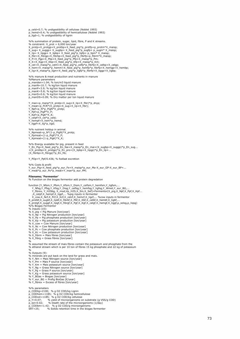
73

p_celd=0.7; % undigestibility of cellulose (Noblet 1993)

p_hemd=0.4; % undigestibility of hemicallulose (Noblet 1993)

p_ligd=1; % undigestibility of lignin

%% summation of protein, sugar, lipid, fibre, P and K streams.

% constraint: X_prot = 6,000 ton/year

X_protp=X_protgp+X_protbp+X_feed_pig*p_protfp+p_protm*X_maisp;

X_sug= X_suggp+ X_sugbp+ X_feed_pig*p_sugfp+ p_sugm* X_maisp;

X_lip= X_lipgp+ X_lipbp+ X_feed_pig*p_lipfp+ p_lipm* X_maisp; X_fibr=X_fibrgp+X_fibrbp+X_feed_pig*p_fibrfp+p_fibrm*X_maisp;

X_P=X_Pgp+X_Pbp+X_feed_pig*p_Pfp+X_maisp*p_Pm;

X_K=X_Kgp+X_Kbp+X_feed_pig*p_Kfp+X_maisp*p_Km;

X_cel=X_maisp*p_celm+X_feed_pig*p_celfp*p_fibrfp+X_celbp+X_celgp; X_hem=X_maisp*p_hemm+X_feed_pig*p_hemfp*p_fibrfp+X_hemgp+X_hembp;

X_lig=X_maisp*p_ligm+X_feed_pig*p_ligfp*p_fibrfp+X_liggp+X_ligbp;

%% manure & meat production and nutrients in manure %Manure parameters

p_manden=1.04; % ton/m3 liquid manure

p_manN=10.7; % kg/ton liquid manure

p_manP=3.9; % kg/ton liquid manure

p_manK=5.8; % kg/ton liquid manure p_manS=0.6; % kg/ton liquid manure

p_manDS=0.09; % Dry matter per ton liquid manure

Y_man=p_manp*(X_protp+X_sug+X_lip+X_fibr)*p_dryp; Y_meat=p_FCR*(X_protp+X_sug+X_lip+X_fibr);

Y_Npf=p_N*p_PigN*X_protp;

Y_Ppf=p_PigP*X_P;

Y_Kpf=p_PigK*X_K; Y_celpf=X_cel*p_celd;

Y_hempf=X_hem*p_hemd;

Y_ligpf=X_lig*p_ligd;

%% nutrient holdup in animal.

Y_Npmeat=p_N*(1-p_PigN)*X_protp;

Y_Ppmeat=(1-p_PigP)*X_P;

Y_Kpmeat=(1-p_PigK)*X_K;

%% Energy available for pig, present in feed

Y_En_Pig=X_feed_pig*p_En_fee+X_maisp*p_En_mai+(X_sugbp+X_suggp)*p_En_sug...

+(X_protbp+X_protgp)*p_En_pro+(X_lipbp+X_lipgp)*p_En_lip+...

(X_fibrbp+X_fibrgp)*p_En_fib;

Y_POp=Y_Ppf/0.436; % fosfaat excretion

%% Costs & profit Y_eur_Pig=X_feed_pig*p_eur_Fe+X_maisp*p_eur_Ma-X_eur_GP-X_eur_BP+...

Y_meat*p_eur_Po*p_meat+Y_man*p_eur_PM;

Filename; ‘Fermentor’

% Function on the biogas fermentor add protein degredation

function [Y_Nfsm,Y_Pfsm,Y_Kfsm,Y_Dism,Y_celfsm,Y_hemfsm,Y_ligfsm,...

Y_Nfsg,Y_Pfsg,Y_Kfsg,Y_Disg,Y_celfsg,Y_hemfsg,Y_ligfsg,Y_Wmet,Y_eur_BG,...

Y_fibrex, Y_H2Sbg, X_mod,Vp_H2S,X_Sin,X_Sef]=Fermentor(X_pig,X_Npf,X_Ppf,X_Kpf... ,X_celpf,X_hempf,X_ligpf,... %pig inputs in fermenter

X_cow,X_Ncf,X_Pcf,X_Kcf,X_celcf,X_hemcf,X_ligcf,... %cow inputs in fermentor

X_protbf,X_sugbf,X_lipbf,X_fibrbf,X_Pbf,X_Kbf,X_celbf,X_hembf,X_ligbf,...

X_protgf,X_suggf,X_lipgf,X_fibrgf,X_Pgf,X_Kgf,X_celgf,X_hemgf,X_liggf,p_solsg,p_liqsg) %% Biogas Fermentor

% Inputs (10):

% X_pig = Pig Manure [ton/year]

% X_Np = Pig Nitrogen production [ton/year] % X_Pp = Pig phosphate production [ton/year]

% X_Kp = Pig potassium production [ton/year]

% X_cow = Cow Manure [ton/year]

% X_Nc = Cow Nitrogen production [ton/year]

% X_Pc = Cow phosphate production [ton/year] % X_Kc = Cow potassium production [ton/year]

% X_fibrm = Mais fibres [ton/year]

% X_fibrg = Grass fibres [ton/year]

% % assumed the stream of mais fibres contain the potassium and phosphate from the

% ethanol stream which is per 10 ton of fibres 15 kg phosphate and 22 kg of potassium

%

% Outputs (9): % minerals are put back on the land for grass and mais.

% Y_Nm = Mais Nitrogen source [ton/year]

% Y_Pm = Mais P source [ton/year]

% Y_Km = Mais potassium source [ton/year]

% Y_Ng = Grass Nitrogen source [ton/year] % Y_Pg = Grass P source [ton/year]

% Y_Kg = Grass potassium source [ton/year]

% Y_BGas = Biogas [ton/year]

% Y_eur_BG = Profig BioGas [€/year] % Y_fibrex = Excess of fibres [ton/year]

%% parameters

p_CODlig=2100; % g O2 COD/kg Lignin p_CODhem=1185; % g O2 COD/kg hemicellulose

p_CODcel=1185; % g O2 COD/kg cellulose

p_Y=0.07; % yield of microorganisms on substrate (g VSS/g COD)

p_kd=0.02; % Death rate of the microorganisms (1/day) p_CODbm=1.42; % g O2 COD/g microorganisms

SRT=25; % Solids retention time in the biogas fermenter

74

p_Vmet=0.4; % Volume of methane at 35 degrees, m3/kg COD

% microorganism composition (weight based)

p_moC=0.5; % carbon in microorganisms p_moO=0.22; % Oxygen in microorganisms

p_moN=0.12; % Nitrogen in microorganisms

p_moH=0.09; % Hydrogen in microorganisms

p_moP=0.02; % Phosphorus in microorganisms

p_moS=0.01; % Sulphur in microorganisms p_moK=0.01; % Potassium in mircroorganisms

%% total mineral production p_N=1/6.25; % kg N per kg protein (all protein)

Y_N=X_Npf+X_Ncf+(X_protbf+X_protgf)*p_N;

Y_P=X_Ppf+X_Pcf+X_Pbf+X_Pgf;

Y_K=X_Kpf+X_Kcf+X_Kbf+X_Kgf;

X_cel=X_celgf+X_celbf+X_celcf+X_celpf;

X_hem=X_hemgf+X_hembf+X_hemcf+X_hempf;

X_lig=X_liggf+X_ligbf+X_ligcf+X_ligpf;

X_CODceli=X_cel*p_CODcel; %COD in the cellulose influent (kg COD/year) X_CODhemi=X_hem*p_CODhem; %COD in the hemicellulose influent (kg COD/year)

X_CODligi=X_lig*p_CODlig; %COD in the ligning influent (kg COD/year)

X_CODin=X_CODceli+X_CODhemi+X_CODligi; % total COD in the influent (kg COD/year)

%% constraints nutrient distribution mais:grass

% nitrogen: mais= 300 grass= 150 kg/ha fraction = 2/3 : 1/3

% phosphate: mais= 50 grass= 40 kg/ha fraction = 5/9 : 4/9

% potassium: mais= 200 grass= 120 kg/ha fraction = 5/8 : 3/8 % note: if blocks are shut down maybe another relation should be used.

% like if(mais,gras,eendenkroos) than distribution= (X:X:X) otherwise....

% mineral production for grass and mais lands

% pN=0.178; % fraction for mais land % pP=0.207; % fraction for mais land

% pK=0.223; % fraction for mais land

% pOM=0.5; % fraction for mais land

% Y_Nfsm=Y_N*pN; % Y_Pfsm=Y_P*pP;

% Y_Kfsm=Y_K*pK;

% Y_Nfsg=Y_N*(1-pN);

% Y_Pfsg=Y_P*(1-pP); % Y_Kfsg=Y_K*(1-pK);

% X_Di=X_cow+X_pig;

%% parameters p_dryp=0.1; %ton dry matter per m3 pig manure (assume density 1000kg/m3)

p_dryc=0.1; %ton dry matter per m3 cow manure (assume density 1000kg/m3)

% subdivision of fibre fraction into cellulose, hemicellulose and lignin

% p_celg=0.250; % Cellulose in grass fibre [kg/kg]

% p_hemg=0.225; % Hemicellulose in grass fibre [kg/kg] % p_ligg=0.025; % Lignin in grass fibre [kg/kg]

% p_celm=0.205; % Cellulose fraciton in mais fibre [kg/kg]

% p_hemm=0.180; % Hemicellulose fraction in mais fibre [kg/kg]

% p_ligm=0.025; % Lignin fraction in mais fibre [kg/kg] % p_celc=0; % Cellulose fraciton in fibre

% p_hemc=0; % Hemicellulose fraction in grass fibre

% p_ligc=0; % Lignin fraction in grass fibre

% p_celp=0; % Cellulose fraciton in grass fibre % p_hemp=0; % Hemicellulose fraction in grass fibre

% p_ligp=0; % Lignin fraction in grass fibre

% Constraint: ratio between pig + cow manure [m3] and dry matter of grass and % mais material [kg] should be

% (X_pig+X_cow):(X_fibrm+X_fibrg+X_sugg+X_protg) = 10 : 1 m3:ton

X_fibrm=X_protbf+X_sugbf+X_lipbf+X_fibrbf; X_fibrg=X_protgf+X_suggf+X_lipgf+X_fibrgf;

X_dryp=X_pig;

X_dryc=X_cow;

if (X_fibrm+X_fibrg-X_dryp-X_dryc)>0

Y_fibrex=X_fibrm+X_fibrg-X_dryp-X_dryc;

else

Y_fibrex=0; end

p_BGasp=0.14; % kg biogass per kg dry pigmanure

p_BGasc=0.10; % kg biogass per kg dry cowmanure

p_BGasf=0.15; % 0.2 with pretreatment % kg biogass per kg fibres p_celd=0.5; % cellulose undigestibility in biofermenter

p_hemd=0.3; % hemicellulose unigestibility in biofermenter

p_ligd=0.75; % lignin undigestibility biofermenter

p_eur_BG= 500; % value of biogas [€/ton] p_eur_Di=-5; % value of digestate [€/m3]

p_eur_Pm= 20; % value of pig manure [€/m3]

p_eur_Cm= 15; % value of cow manure [€/m3]

p_eur_Gf=-360; % Value of Grass Fibres [€/ton] p_eur_Mf=-285; % Value of Mais Fibres [€/ton]

p_eur_Fi= 360; % value excess Fibres [€/ton]

p_proces=-100; % process costs Fibres [€/ton]

X_CODcele=p_celd*X_CODceli; %Cellulose COD in the effluent

X_CODheme=p_hemd*X_CODhemi; %Hemicellulose COD in the effluent

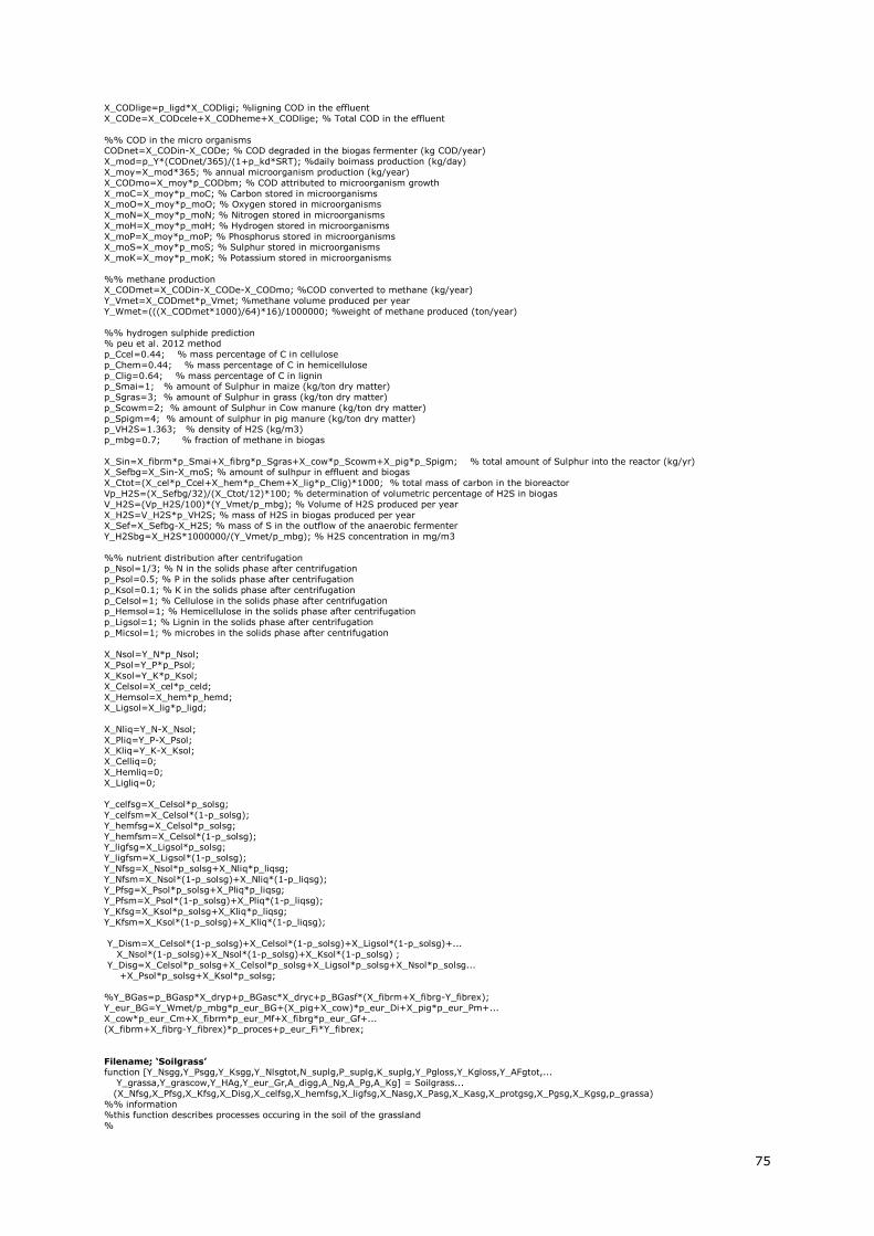
75

X_CODlige=p_ligd*X_CODligi; %ligning COD in the effluent

X_CODe=X_CODcele+X_CODheme+X_CODlige; % Total COD in the effluent

%% COD in the micro organisms CODnet=X_CODin-X_CODe; % COD degraded in the biogas fermenter (kg COD/year)

X_mod=p_Y*(CODnet/365)/(1+p_kd*SRT); %daily boimass production (kg/day)

X_moy=X_mod*365; % annual microorganism production (kg/year)

X_CODmo=X_moy*p_CODbm; % COD attributed to microorganism growth

X_moC=X_moy*p_moC; % Carbon stored in microorganisms X_moO=X_moy*p_moO; % Oxygen stored in microorganisms

X_moN=X_moy*p_moN; % Nitrogen stored in microorganisms

X_moH=X_moy*p_moH; % Hydrogen stored in microorganisms

X_moP=X_moy*p_moP; % Phosphorus stored in microorganisms X_moS=X_moy*p_moS; % Sulphur stored in microorganisms

X_moK=X_moy*p_moK; % Potassium stored in microorganisms

%% methane production X_CODmet=X_CODin-X_CODe-X_CODmo; %COD converted to methane (kg/year)

Y_Vmet=X_CODmet*p_Vmet; %methane volume produced per year

Y_Wmet=(((X_CODmet*1000)/64)*16)/1000000; %weight of methane produced (ton/year)

%% hydrogen sulphide prediction % peu et al. 2012 method

p_Ccel=0.44; % mass percentage of C in cellulose

p_Chem=0.44; % mass percentage of C in hemicellulose

p_Clig=0.64; % mass percentage of C in lignin p_Smai=1; % amount of Sulphur in maize (kg/ton dry matter)

p_Sgras=3; % amount of Sulphur in grass (kg/ton dry matter)

p_Scowm=2; % amount of Sulphur in Cow manure (kg/ton dry matter)

p_Spigm=4; % amount of sulphur in pig manure (kg/ton dry matter) p_VH2S=1.363; % density of H2S (kg/m3)

p_mbg=0.7; % fraction of methane in biogas

X_Sin=X_fibrm*p_Smai+X_fibrg*p_Sgras+X_cow*p_Scowm+X_pig*p_Spigm; % total amount of Sulphur into the reactor (kg/yr) X_Sefbg=X_Sin-X_moS; % amount of sulhpur in effluent and biogas

X_Ctot=(X_cel*p_Ccel+X_hem*p_Chem+X_lig*p_Clig)*1000; % total mass of carbon in the bioreactor

Vp_H2S=(X_Sefbg/32)/(X_Ctot/12)*100; % determination of volumetric percentage of H2S in biogas

V_H2S=(Vp_H2S/100)*(Y_Vmet/p_mbg); % Volume of H2S produced per year

X_H2S=V_H2S*p_VH2S; % mass of H2S in biogas produced per year X_Sef=X_Sefbg-X_H2S; % mass of S in the outflow of the anaerobic fermenter

Y_H2Sbg=X_H2S*1000000/(Y_Vmet/p_mbg); % H2S concentration in mg/m3

%% nutrient distribution after centrifugation p_Nsol=1/3; % N in the solids phase after centrifugation

p_Psol=0.5; % P in the solids phase after centrifugation

p_Ksol=0.1; % K in the solids phase after centrifugation

p_Celsol=1; % Cellulose in the solids phase after centrifugation p_Hemsol=1; % Hemicellulose in the solids phase after centrifugation

p_Ligsol=1; % Lignin in the solids phase after centrifugation

p_Micsol=1; % microbes in the solids phase after centrifugation

X_Nsol=Y_N*p_Nsol; X_Psol=Y_P*p_Psol;

X_Ksol=Y_K*p_Ksol;

X_Celsol=X_cel*p_celd;

X_Hemsol=X_hem*p_hemd; X_Ligsol=X_lig*p_ligd;

X_Nliq=Y_N-X_Nsol;

X_Pliq=Y_P-X_Psol; X_Kliq=Y_K-X_Ksol;

X_Celliq=0;

X_Hemliq=0;

X_Ligliq=0;

Y_celfsg=X_Celsol*p_solsg;

Y_celfsm=X_Celsol*(1-p_solsg);

Y_hemfsg=X_Celsol*p_solsg;

Y_hemfsm=X_Celsol*(1-p_solsg); Y_ligfsg=X_Ligsol*p_solsg;

Y_ligfsm=X_Ligsol*(1-p_solsg);

Y_Nfsg=X_Nsol*p_solsg+X_Nliq*p_liqsg;

Y_Nfsm=X_Nsol*(1-p_solsg)+X_Nliq*(1-p_liqsg); Y_Pfsg=X_Psol*p_solsg+X_Pliq*p_liqsg;

Y_Pfsm=X_Psol*(1-p_solsg)+X_Pliq*(1-p_liqsg);

Y_Kfsg=X_Ksol*p_solsg+X_Kliq*p_liqsg;

Y_Kfsm=X_Ksol*(1-p_solsg)+X_Kliq*(1-p_liqsg);

Y_Dism=X_Celsol*(1-p_solsg)+X_Celsol*(1-p_solsg)+X_Ligsol*(1-p_solsg)+...

X_Nsol*(1-p_solsg)+X_Nsol*(1-p_solsg)+X_Ksol*(1-p_solsg) ;

Y_Disg=X_Celsol*p_solsg+X_Celsol*p_solsg+X_Ligsol*p_solsg+X_Nsol*p_solsg...

+X_Psol*p_solsg+X_Ksol*p_solsg;

%Y_BGas=p_BGasp*X_dryp+p_BGasc*X_dryc+p_BGasf*(X_fibrm+X_fibrg-Y_fibrex);

Y_eur_BG=Y_Wmet/p_mbg*p_eur_BG+(X_pig+X_cow)*p_eur_Di+X_pig*p_eur_Pm+...

X_cow*p_eur_Cm+X_fibrm*p_eur_Mf+X_fibrg*p_eur_Gf+... (X_fibrm+X_fibrg-Y_fibrex)*p_proces+p_eur_Fi*Y_fibrex;

Filename; ‘Soilgrass’ function [Y_Nsgg,Y_Psgg,Y_Ksgg,Y_Nlsgtot,N_suplg,P_suplg,K_suplg,Y_Pgloss,Y_Kgloss,Y_AFgtot,...

Y_grassa,Y_grascow,Y_HAg,Y_eur_Gr,A_digg,A_Ng,A_Pg,A_Kg] = Soilgrass...

(X_Nfsg,X_Pfsg,X_Kfsg,X_Disg,X_celfsg,X_hemfsg,X_ligfsg,X_Nasg,X_Pasg,X_Kasg,X_protgsg,X_Pgsg,X_Kgsg,p_grassa)

%% information %this function describes processes occuring in the soil of the grassland

%

76

% inputs

% X_Nfsg = Nitrogen from fermentor to Grassland[ton N/year]

% X_Pfsg = phosphorous from fermentor to Grassland [ton P/year]

% X_Kfsg = Potassium from fermentor to Grassland [ton K/year] % X_Disg = Volume from fermentor to Grassland [m3/year]

% X_Nasg = Nitrogen in artificial fertilizer [ton N/year]

% X_Pasg = phosphorous in artificial fertilizer [ton P/year]

% X_Kasg = Potassium in artificial fertilizer [ton K/year]

% X_protgsg = protein in grass juice from grassa [ton protein/year] % X_Pgsg = phosphorous in grass juice from grassa [ton P/year]

% X_Kgsg = Potassium in grass juice from grassa [ton K/year]

%

% Outputs %

% Y_Nsgg = Nitrogen from grassland to grass

% Y_Psgg = Phosphorus from grassland to grass

% Y_Ksgg = Potassium from grassland to grass %

%% Parameters

% wash out,N2 loss, NH4 loss.

% numbers still need to be included

p_DMgras=0.2; % dry matter percentage of grass p_N=.0336; % Load of minerals [ton/ton crops]

p_P=.0035; % Load of minerals [ton/ton crops]

p_K=.025; % Load of minerals [ton/ton crops]

p_grass= 10; % grass yield per hectare [ton grassDM/ha] p_AF=0.3; % effective mass of fertilizer

% Soil parameters

P_Nwo=0.25; %0.20-0.35 MMM Nitrate washout P_NN2=0.0; %0.10-0.25 MMM Denitrification

P_NNH4=0.0; %0-0.1 MMM Ammonium Volatilisation

P_NGrass=0.75; %0.4-0.6 MMM Nutrient uptake by crop

P_PGrass=0.90; % nutrient uptake by crop P_Ploss=0.10; % nutrient loss

P_KGrass=0.9; % nutrient uptake by crop

P_Kloss=0.1; % nutrient loss

P_Nfix=500; % tonnes N from Biological Nitrogen fixation legumes

% prices

p_grascow=1-p_grassa; % fraction of grass for cow

p_grass= 10; % grass yield per hectare [ton grassDM/ha]

p_eur_Gr= 250; % grass value per ton DM [€/ton DM] p_eur_AF=-420; % Artifical fertilizer value [€/ton] (costs=negative)

p_eur_Di= 5; % Digestate costs [€/DM]

p_eur_Ju=-1200; % Value of phosphorous in juice [€/ton]

%% total amount of nutrients applied on the soil

X_Ntot=X_Nfsg+X_Nasg+X_protgsg/6.25+P_Nfix; % 6.25 kg protein : 1 kg N

X_Ptot=X_Pfsg+X_Pasg+X_Pgsg;

X_Ktot=X_Kfsg+X_Kasg+X_Kgsg;

%% Nutrient distrubution

Y_Nsgg=P_NGrass*X_Ntot;

Y_Ngwo=P_Nwo*X_Ntot;

Y_NgN2=P_NN2*X_Ntot; Y_NgNH4=P_NNH4*X_Ntot;

Y_Psgg=P_PGrass*X_Ptot;

Y_Ksgg=P_KGrass*X_Ktot;

Y_AFgtot=X_Nasg+X_Pasg/0.436+X_Kasg/0.83; % 0.436 is the amount of P in P2O5, and 0.83 is the amount of K in KO2

%% expected crop growth:

Y_grass=min([Y_Nsgg/p_N;Y_Psgg/p_P;Y_Ksgg/p_K]);

N_suplg=Y_Nsgg-(Y_grass*p_N); % check if there is a surplus of N P_suplg=Y_Psgg-(Y_grass*p_P); % check if there is a surplus of P

K_suplg=Y_Ksgg-(Y_grass*p_K); % check if there is a surplus of K

% include surpluss in the losses

Y_Nlsgtot=Y_Ngwo+Y_NgN2+Y_NgNH4+N_suplg; Y_Pgloss=X_Ptot*P_Ploss+P_suplg;

Y_Kgloss=X_Ktot*P_Kloss+K_suplg;

Y_HAg=Y_grass/p_grass; % # of hectares which can be supplied with nutrients, Y_eur_Gr=Y_grass*p_eur_Gr+(Y_AFgtot)/p_AF*p_eur_AF+X_Disg*p_eur_Di+X_Pgsg*p_eur_Ju; % [€/year]

Y_grassa=Y_grass*p_grassa;

Y_grascow=Y_grass*p_grascow;

% Fertilization rates

A_digg=(X_celfsg+X_hemfsg+X_ligfsg)/Y_HAg; %application rate lignocellulose material from fermenter

A_Ng=X_Ntot/Y_HAg; % application rate of N on soil

A_Pg=X_Ptot/Y_HAg; % application rate of P on soil

A_Kg=X_Ktot/Y_HAg; % application rate of K on soil

end

Filename; ‘Soilmaize’ function [Y_Nsmm,Y_Psmm,Y_Ksmm,Y_Nlmgtot,N_suplm,P_suplm,K_suplm,Y_Pmloss,Y_Kmloss,Y_AFmtot,...

Y_Maisb,Y_Maisc,Y_Maisp,Y_HAm,Y_eur_Ma,A_digm,A_Nm,A_Pm,A_Km] = Soilmaize...

(X_Nfsm,X_Pfsm,X_Kfsm,X_Dism,X_celfsm,X_hemfsm,X_ligfsm,X_Nasm,X_Pasm,X_Kasm,X_protbsm,X_Pbsm,X_Kbsm,...

p_byos,p_mcow,p_mpig) %% information

% this function descibes the processes occuring in the soil of maizeland

% Inputs % X_Nfsm = Nitrogen from fermentor to Maizeland[ton N/year]

% X_Pfsm = phosphorous from fermentor to maizeland [ton P/year]

77

% X_Kfsm = Potassium from fermentor to maizeland [ton K/year]

% X_Dism = Volume from fermentor to maizeland [m3/year]

% X_Nasm = Nitrogen in artificial fertilizer [ton N/year]

% X_Pasm = phosphorous in artificial fertilizer [ton P/year] % X_Kasm = Potassium in artificial fertilizer [ton K/year]

% X_protbsm = protein in grass juice from grassa [ton protein/year]

% X_Pbsm = phosphorous in grass juice from grassa [ton P/year]

% X_Kbsm = Potassium in grass juice from grassa [ton K/year]

% % Outputs

% Y_Nsmm = Nitrogen from maizeland to maize

% Y_Psmm = Phosphorus from maizeland to maize

% Y_Ksmm = Potassium from maizeland to maize

%% Parameters

% wash out,N2 loss, NH4 loss.

% loss according to MMM, for sand soils p_N=.010; % Load of minerals [ton/ton crops]

p_P=.0019; % Load of phosphorous [ton/ton crops]

p_K=.010; % Load of potassium [ton/ton crops]

p_mais=17; % mais yield per hectare [ton mais DM/ha]

p_DMmais=0.32; % dry matter maize plant % soil losses

P_Nwo=0.25; %0.20-0.35 MMM

P_NN2=0; %0.10-0.25 MMM

P_NNH4=0.0; %0-0.1 MMM P_NMaize=0.75; %0.4-0.6 MMM

P_PMaize=0.90;

P_Ploss=0.10;

P_KMaize=0.9; P_Kloss=0.1;

p_AF=0.3; % effective mass of fertilizer

p_eur_Ma= 180; % Mais price per ton DM [€/ton] p_eur_AF=-420; % Artifical fertilizer costs [€/ton] (costs=negative)

p_eur_Di= 5; % Digestate [€/DM]

p_eur_Ju=-2000; % Value of phosphorous [€/ton](costs=negative)

%% total nutrients X_Ntot=X_Nfsm+X_Nasm+X_protbsm/6.25;% 6.25 kg protein : 1 kg N

X_Ptot=X_Pfsm+X_Pasm+X_Pbsm;

X_Ktot=X_Kfsm+X_Kasm+X_Kbsm;

%% Nutrient distrubution

Y_Nsmm=P_NMaize*X_Ntot;

Y_Psmm=P_PMaize*X_Ptot;

Y_Ksmm=P_KMaize*X_Ktot; Y_Nmwo=P_Nwo*X_Ntot;

Y_NmN2=P_NN2*X_Ntot;

Y_NmNH4=P_NNH4*X_Ntot;

Y_Nlmgtot=Y_NmNH4+Y_NmN2+Y_Nmwo;

Y_AFmtot=X_Nasm+X_Pasm/0.436+X_Kasm/0.83; % 0.436 is the amount of P in P2O5, and 0.83 is the amount of K in KO2

%% excpeted Maize production

Y_Mais=min([Y_Nsmm/p_N;Y_Psmm/p_P;Y_Ksmm/p_K]); % [ton/year]

N_suplm=Y_Nsmm-(Y_Mais*p_N); P_suplm=Y_Psmm-(Y_Mais*p_P);

K_suplm=Y_Ksmm-(Y_Mais*p_K);

Y_Nlsmtot=Y_Nmwo+Y_NmN2+Y_NmNH4+N_suplm; Y_Pmloss=X_Ptot*P_Ploss+P_suplm;

Y_Kmloss=X_Ktot*P_Kloss+K_suplm;

Y_HAm=Y_Mais/p_mais; % # of hectares which can be supplied with nutrients Y_eur_Ma=Y_Mais*p_eur_Ma+(Y_AFmtot)/p_AF*p_eur_AF+X_Dism*p_eur_Di+X_Pbsm*p_eur_Ju; % [€/year]

Y_Maisb=Y_Mais*p_byos;

Y_Maisc=Y_Mais*p_mcow;

Y_Maisp=Y_Mais*p_mpig;

% fertilization rates

A_digm=X_Dism/Y_HAm;

A_Nm=X_Ntot/Y_HAm;

A_Pm=X_Ptot/Y_HAm; A_Km=X_Ktot/Y_HAm;

end

filename; ‘Datagen’

%% all outputs Byosense

clear all

close all clc

load 'xbest.mat'

xopt=xbest;

delete 'data' diary data

[X_protbf,X_sugbf,X_lipbf,X_fibrbf,X_Pbf,X_Kbf,X_celbf,X_hembf,X_ligbf... %byosense-fermentor

X_protbc,X_sugbc,X_lipbc,X_fibrbc,X_Pbc,X_Kbc,X_celbc,X_hembc,X_ligbc... %byosense-cow X_protbp,X_sugbp,X_lipbp,X_fibrbp,X_Pbp,X_Kbp,X_celbp,X_hembp,X_ligbp... %byosense-pig

X_protbsm,X_sugbsm,X_lipbsm,X_fibrbsm,X_Pbsm,X_Kbsm,X_celbsm,X_hembsm,X_ligbsm... %byosense-maisland

Y_eth,Y_eur_Byo,X_eur_BC,X_eur_BP]=Byosense(xopt(9),xopt(14),0)

78

%% all outputs Grassa

[X_protgc,X_suggc,X_lipgc,X_fibrgc,X_Pgc,X_Kgc,X_celgc,X_hemgc,X_liggc,... %Grassa-cow

X_protgp,X_suggp,X_lipgp,X_fibrgp,X_Pgp,X_Kgp,X_celgp,X_hemgp,X_liggp,... %Grassa-pig X_protgf,X_suggf,X_lipgf,X_fibrgf,X_Pgf,X_Kgf,X_celgf,X_hemgf,X_liggf,... %Grassa-fermentor

X_protgsg,X_suggsg,X_lipgsg,X_fibrgsg,X_Pgsg,X_Kgsg,X_celgsg,X_hemgsg,X_liggsg... %Grassa-grassland

,Y_eur_GA,X_eur_GC,X_eur_GP]=GRASSA(xopt(12),xopt(19),xopt(20),xopt(23))

%% all outputs cow

[X_Ncf,X_Pcf,X_POc,X_Kcf,X_cow,X_celcf,X_hemcf,X_ligcf,Y_Nmeat,Y_Pmeat,Y_Kmeat,...

Y_Nmilk,Y_Pmilk,Y_Kmilk,Y_En_Cow,Y_eur_Cow,X_protc]=Cow...

(xopt(1),xopt(10),xopt(13),...% concentrates & roughage X_eur_GC,X_protgc,X_suggc,X_lipgc,X_fibrgc,X_Pgc,X_Kgc,X_celgc,X_hemgc,X_liggc,... % Grassa-cow

X_eur_BC,X_protbc,X_sugbc,X_lipbc,X_fibrbc,X_Pbc,X_Kbc,X_celbc,X_hembc,X_ligbc) % Byosense-cow

%% all outputs pig

[X_Npf,X_Ppf,X_POp,X_Kpf,X_pig,X_celpf,X_hempf,X_ligpf,Y_meat,Y_Npmeat,Y_Ppmeat,Y_Kpmeat,...

Y_En_Pig,Y_eur_Pig,X_protp]=Pig(xopt(11),xopt(2),...

X_eur_GP,X_protgp,X_suggp,X_lipgp,X_fibrgp,X_Pgp,X_Kgp,X_celgp,X_hemgp,X_liggp,... %Grassa-pig

X_eur_BP,X_protbp,X_sugbp,X_lipbp,X_fibrbp,X_Pbp,X_Kbp,X_celbp,X_hembp,X_ligbp) %Byosense-pig

%% all outputs Fermentor

[X_Nfsm,X_Pfsm,X_Kfsm,X_Dism,X_celfsm,X_hemfsm,X_ligfsm... ,X_Nfsg,X_Pfsg,X_Kfsg,X_Disg,X_celfsg,X_hemfsg,X_ligfsg,Y_Wmet,Y_eur_BG,Y_fibrex,...

Y_H2Sbg,X_mod,Vp_H2S,X_Sin,X_Sef]...

=Fermentor(X_pig,X_Npf,X_Ppf,X_Kpf,X_celpf,X_hempf,X_ligpf,...

X_cow,X_Ncf,X_Pcf,X_Kcf,X_celcf,X_hemcf,X_ligcf,... X_protbf,X_sugbf,X_lipbf,X_fibrbf,X_Pbf,X_Kbf,X_celbf,X_hembf,X_ligbf,... % Byosense-fermentor

X_protgf,X_suggf,X_lipgf,X_fibrgf,X_Pgf,X_Kgf,X_celgf,X_hemgf,X_liggf,xopt(21),xopt(22))

%% all outputs grass [X_Nsgg,X_Psgg,X_Ksgg,Y_Nlsgtot,N_suplg,P_suplg,K_suplg,Y_Pgloss,Y_Kgloss,Y_AFgtot,...

Y_Grassa,Y_Grascow,Y_HAg,Y_eur_Gr,A_digg,A_Ng,A_Pg,A_Kg] = Soilgrass...

(X_Nfsg,X_Pfsg,X_Kfsg,X_Disg,X_celfsg,X_hemfsg,X_ligfsg,xopt(6),xopt(7),xopt(8),X_protgsg,X_Pgsg,X_Kgsg,xopt(15))

%% all outputs Maize

[X_Nsmm,X_Psmm,X_Ksmm,X_Nlmgtot,N_suplm,P_suplm,K_suplm,Y_Pmloss,Y_Kmloss,Y_AFmtot,...

Y_Maisb,Y_Maisc,Y_Maisp,Y_HAm,Y_eur_Ma,A_digm,A_Nm,A_Pm,A_Km] = Soilmaize...

(X_Nfsm,X_Pfsm,X_Kfsm,X_Dism,X_celfsm,X_hemfsm,X_ligfsm,xopt(3),xopt(4),xopt(5),X_protbsm,X_Pbsm,X_Kbsm,... xopt(16),xopt(17),xopt(18))

xopt

diary off

xlswrite('xbest.xlsx',xopt)

filename; ‘Csoilrun’

% define parameters

k1=2; % decomposition rate constant of fast decomposing material

k2=0.2; % decomposition rate constant of slow decomposing material

k3=0.02; % decomposition rate constant of hummus/biomass k=[k1;k2;k3];

adig=3.7; % apparent age of the digestate based on janssen 1996 table 7

afer=1; % apperant age of the fertilizer tsim=0:0.1:20; % time scale of the simulation

% input parameters:

%LOAD OPTIMIZED MODEL PARAMETERS AND CALCULATE THE FERTILIZATION RATIO!!!

Adig=1.58; % influx digestate in ton per hectare based on optimized model output

Afer=0; % influx fertilizer in ton per hectare based on optimized model output

% determination of initial destribution between fast and slow decomposing % compartments (equations taken from Janssen 1996 and groenendijk 2005)

p(1)=-0.0105*adig^3+0.1394*adig^2-0.6904*adig+1.4767;

ep(1)=-0.0066*adig^3+0.0673*adig^2-0.1096*adig+0.0705;

p(2)=-0.0105*afer^3+0.1394*afer^2-0.6904*afer+1.4767; ep(2)=-0.0066*afer^3+0.0673*afer^2-0.1096*afer+0.0705;

% soil organic matter distribution

% it is assumed the inital distribution of digestate and fertilizer is 1:1

C_org=52; % Organic ton organic matter/hectare

p_hum=0.9; % fraction of organic matter attributed to hummes (groenendijk et al. 2005)

p_new=0.1; % fraction of organic matter attributed to fresh organic matter

C_hum=C_org*p_hum; % initial amount of humus in the top soil layer

C_fast=((p(1)*0.5)+(p(2)*0.5))*p_new*C_org % ton per hectare

C_slow=(((1-p(1))*0.5+((1-p(2))*0.5)))*p_new*C_org % ton per hectare

C0=[C_fast;C_slow;C_hum];

[T,Y]=ode45(@Csoil2,tsim,C0,[],k,Adig,Afer,adig,afer);

Y(:,4)=Y(:,1)+Y(:,2)+Y(:,3);

figure(1)

plot(T,Y(:,1),T,Y(:,2),T,Y(:,3),T,Y(:,4))

legend('fast decomposing material','slow decomposing material','biomass/humus','total SOM') xlabel('time (year)');

ylabel('mass (ton/hectare)');

79

filename; ‘Csoil2’

function Cp = Csoil2(t,C,k,Adig,Afer,adig,afer)

p1=-0.0105*adig(1)^3+0.1394*adig(1)^2-0.6904*adig(1)+1.4767; %charactarization of different materials

ep1=-0.0066*adig(1)^3+0.0673*adig(1)^2-0.1096*adig(1)+0.0705;

p2=-0.0105*afer(1)^3+0.1394*afer(1)^2-0.6904*afer(1)+1.4767;

ep2=-0.0066*afer(1)^3+0.0673*afer(1)^2-0.1096*afer(1)+0.0705;

p=[p1;p2]';

ep=[ep1;ep2];

B=[p(1)*Adig+p(2)*Afer;p(1)*Adig+p(2)*Afer;0];

%Cp=[-k(1) 0 0;0 -k(2) 0;ep*k(1) ep*k(2) -k(3)]*C+B

Cp=[-k(1) 0 0 ;... 0 -k(2) 0 ;...

ep(1)*k(1)+ep(2)*k(1) ep(1)*k(2)+ep(2)*k(2) -k(3)]*C+B;

% Cp(1)=*Cp(1)+B(1);

% Cp(2)=*Cp(2)+B(2); % Cp(3)=*Cp(3)+B(3);

% Cp(4)=-k(2)*Cp(4)+B(4);

% Cp(5)=ep(1)*k(1)*Cp(1)+ep(1)*k(2)*Cp(2)+ep(2)*k(1)*Cp(3)+ep(2)*k(2)*Cp(4)-k(3)*Cp(5);