Modelling of Dynamic Edge Loading in Total Hip ...etheses.whiterose.ac.uk/19913/7/Jahani_F_Mechanical_PhD...Modelling of Dynamic Edge Loading in Total Hip Replacements with ceramic

I

Modelling of Dynamic Edge Loading in Total Hip

Replacements with ceramic on polyethylene

Bearings

By

Faezeh Jahani

Submitted in accordance with the requirements for the degree of Doctor of Philosophy

The University of Leeds School of Mechanical Engineering

September, 2017

II

The candidate confirms that the work submitted is her own, except where work

which has formed part of jointly-authored publications has been included. The

contribution of the candidate and the other authors to this work has been explicitly

indicated below. The candidate confirms that appropriate credit has been given

within the thesis where reference has been made to the work of others.

This copy has been supplied on the understanding that it is copyright material and

that no quotation from the thesis may be published without proper

acknowledgement.

© 2017 The University of Leeds and Faezeh Jahani

The right of Faezeh Jahani to be identified as Author of this work has been asserted

by her in accordance with the Copyright, Designs and Patents Act 1988.

III

Acknowledgement

My first appreciation goes to the brilliant supervision team that I had the pleasure

to work with. Prof. Ruth Wilcox, Dr Alison Jones, Prof. David Barton and Prof John

Fisher, thank you for such an amazing opportunity and believing in me. This piece

of work is the mirror of the amazing effort of my supervisor Dr Alison Jones who

guided and supported me throughout my PhD not only professionally but also

emotionally. She wisely provided the emotional support in the times that I needed

understanding. I also like to thank Mr James Brooks who was a great help to my

project.

My appreciation goes to EPSRC and DePuy Synthes for providing funding for me to

be able to finish this PhD.

My family gave me the motivation to go for the biggest achievement of my life. I am

genuinely indebted to my father, Sadegh Jahani, my mother, Fatemeh Sharei and my

sister, Razieh Jahani for the hardships I caused them to peruse my dream. I hope this

thesis could make them proud. My other sister, Massoumeh Jahani not only has been

a family to me throughout this journey, she also has been a mentor. Simply thank

you for everything you have done for me. I also like to thank my niece and my

nephew, Arina Saeid and Radin Ahmadi, for understanding all those weekends of

work instead of playing time with them.

I am blessed not only because of having a supportive supervisors and family, but

also, for the amazing friends who listened to my complaints and reminded me of my

goal. Behnaz Bazmi and Bahare Mousaei, especially thank you for your timeless

kindness. My special thanks goes to my rock, Matthew Smith, who is the biggest

blessing of my life. I am humbly grateful firstly for understanding my frustrations

IV

every time I didn’t get the result I wanted and secondly, for every little effort you

made to make me feel I can do this.

I worked in a very supportive environment the support of experimental studies

experts, Mazen Al-Hajjar and Murat Ali, can’t be forgotten. Also special thanks to

everyone in room X301 for kind and enjoyable atmosphere to work in.

I believe in the greatest power who brought all these people to my life and showed

me the path I am taking. Thank you God.

V

Abstract

The performance of total hip replacement (THR) devices can be affected by various

factors such as quality of the tissues surrounding the joint, mismatch of the

component centres or the cup positioning during hip replacement surgery.

Experimental studies have shown that these factors can cause the separation of the

two components during the walking cycle (dynamic separation) and the contact of

the femoral head with the rim of the acetabular liner (edge loading), which can lead

to increased wear and shortened implant lifespan.

There is a need for flexible pre-clinical testing tools which allow THR devices to be

assessed under these adverse conditions. In this work, a novel dynamic finite

element model was developed that is able to generate dynamic separation as it

occurs during the gait cycle. In addition, the ability to interrogate contact mechanics

and material strain under separation conditions provides a unique means of

assessing the severity of edge loading. This study demonstrates these model

capabilities for a range of simulated surgical translational mismatch values, cup

inclination angles and swing phase loads for ceramic-on-polyethylene implants.

The computational model was developed to replicate one station of the Leeds II hip

simulator that mimic in vitro adverse conditions. Firstly, a computational sensitivity

model was developed under standard conditions for a stable computational contact.

The mechanism of separation was also added. The finite element model was able to

predict medial-lateral separation as it occurred dynamically in the gait cycle,

including cases where the femoral head was in contact with the rim of the cup. The

increase in medial-lateral separation with increased translational mismatch, cup

inclination angle and decreased swing phase load were in broad agreement with

existing experimental data.

VI

The factors that increased the separation level, also increased the permeant

deformation on the cup. However, steep cup inclination angle resulted in a higher

number of conditions with permanent deformation than the standard cup

inclination angle. Moreover, despite the low axial load during swing phase, under

some separation conditions, reduced contact area created stress value higher than

those at the peak axial load.

The developed computational tool can be used to understand the effect of various

factors on the separation and contact mechanics simultaneously. As separation is a

multi-factorial phenomenon, this model can assist to focus on the selected factors

that affect the separation experimentally. Moreover, the effect of components

specifications such as materials, geometry, and the cup thickness can be investigated

with this model.

VII

Table of contents

Acknowledgement .............................................................................................................................. III

Abstract ................................................................................................................................................... V

Table of Figures ................................................................................................................................ XIII

Chapter 1 Introduction and Literature review .................................................................. 1

1.1 Introduction ........................................................................................................................ 1

1.2 THR design and performance ....................................................................................... 2

1.2.1 Gait Cycle ............................................................................................................................................. 4

1.2.2 Hip disorders ..................................................................................................................................... 4

1.2.3 Total hip replacement (THR) ...................................................................................................... 5

1.2.4 Types of hip replacements ........................................................................................................... 7

1.2.5 Gait cycle of THRs ......................................................................................................................... 10

1.2.6 Failure of hip replacements ...................................................................................................... 12

1.2.7 Dynamic separation ..................................................................................................................... 14

1.2.8 Positioning of THR........................................................................................................................ 17

1.3 Tribology of artificial hip joint ................................................................................... 20

1.3.1 Wear ................................................................................................................................................... 20

1.3.3 Friction and Lubrication ....................................................................................................... 27

1.3.3 Contact mechanics ................................................................................................................... 29

1.4 Computational studies .................................................................................................. 32

1.4.1 Finite element modelling of THRs ......................................................................................... 34

1.4.2 Two-Dimensional hip models .................................................................................................. 35

1.4.3 Axisymmetric hip models .......................................................................................................... 36

VIII

1.4.4 Three-Dimensional hip models under idealised condition ......................................... 38

1.4.5 Three dimensional hip models under microseparation condition .......................... 41

1.4.6 Coupling of dynamic and contact mechanic analysis ..................................................... 47

1.4.7 THR dynamic modelling ............................................................................................................. 50

1.4.8 Wear modelling ............................................................................................................................. 53

1.5 Summary ............................................................................................................................ 53

1.6 Aims and objective.......................................................................................................... 55

Chapter 2 Development of the explicit model under concentric loading

conditions 59

2.1 Introduction ...................................................................................................................... 59

2.2 Experimental setup of Leeds II hip simulator ...................................................... 60

2.3 Design of numerical study ........................................................................................... 62

2.4 Methods of Numerical Analysis .................................................................................. 64

2.4.1 Dynamic solving processors ................................................................................................ 64

2.4.2 Contact algorithms .................................................................................................................. 66

2.5 Development of the Numerical Model ..................................................................... 70

2.5.1 Materials ...................................................................................................................................... 70

2.5.2 Study I: mesh sensitivity analysis...................................................................................... 74

2.5.3 Study II: Contact methods .................................................................................................... 76

2.5.4 Study III: Loading ..................................................................................................................... 76

2.6 Results of concentric loading condition ................................................................. 78

2.6.1 Study I: Mesh sensitivity analysis ...................................................................................... 78

2.6.2 Study II: Contact methods .................................................................................................... 86

IX

2.6.3 Study III: Loading condition ................................................................................................ 89

2.7 Discussion .......................................................................................................................... 93

2.8 Key points .......................................................................................................................... 95

Chapter 3 Model development under adverse conditions ......................................... 97

3.1 Introduction ...................................................................................................................... 97

3.2 Technical Background ................................................................................................ 100

3.2.1 Stability and time incrementation ..................................................................................101

3.2.2 An oscillatory system ...........................................................................................................104

3.3 Materials and methods .............................................................................................. 107

3.3.1 Geometry and alignment .....................................................................................................107

3.3.2 Assembly ....................................................................................................................................107

3.3.3 Material properties ...............................................................................................................108

3.3.4 Finite element mesh ..............................................................................................................110

3.3.5 Methods ......................................................................................................................................111

3.3.6 Spring representation ..........................................................................................................113

3.3.7 Boundary conditions, loads and analysis steps .........................................................114

3.3.8 Inclusion of damping ............................................................................................................117

3.3.9 Mass effect .................................................................................................................................118

3.3.10 Model input sensitivity ...................................................................................................119

3.3.11 Model output measures..................................................................................................120

3.4 Results .............................................................................................................................. 121

3.4.1 Spring representation ..........................................................................................................121

3.4.2 Inclusion of damping ............................................................................................................123

X

3.4.3 Mass effect .................................................................................................................................128

3.4.4 Model input sensitivity ........................................................................................................130

3.5 Discussion ....................................................................................................................... 132

3.6 Key findings .................................................................................................................... 136

Chapter 4 Parametric sweep, validation and sensitivity testing .......................... 137

4.1 Introduction ................................................................................................................... 137

4.2 Methodology .................................................................................................................. 139

4.2.1 Input parameters ...................................................................................................................141

4.2.2 Outputs and experimental comparison ........................................................................145

4.2.3 Friction sensitivity test ........................................................................................................147

4.3 Results .............................................................................................................................. 148

4.3.1 In silico parameter sweep ...................................................................................................148

4.3.2 Comparison of in vitro and in silico .................................................................................152

4.3.3 Friction sensitivity test ........................................................................................................156

4.3.4 Maximum load at the rim ....................................................................................................157

4.4 Discussion ....................................................................................................................... 165

4.4.1 Computational results ..........................................................................................................166

4.4.2 Validation ..................................................................................................................................168

4.4.3 Friction sensitivity analysis ...............................................................................................173

4.4.4 Summary of the key findings .............................................................................................173

Chapter 5 Parametric sweep contact mechanics analyses ..................................... 175

5.1 Introduction ................................................................................................................... 175

5.2 Methodology ......................................................................................................................... 176

XI

5.3 Results ..................................................................................................................................... 181

5.3.1 Input parameters study .......................................................................................................181

5.3.2 Material failure risk ...............................................................................................................188

5.3.3 Separation study .....................................................................................................................200

5.3.4 Friction .......................................................................................................................................203

5.4 Discussion .............................................................................................................................. 209

5.4.1 Contact behaviour due to the input parameters ............................................................209

5.4.2 Discussion of stress behaviour throughout gait cycle .................................................210

5.4.3 Failure Prediction .......................................................................................................................213

5.4.4 The correlation between separation and contact mechanics ...................................215

5.4.5 Friction effect ...............................................................................................................................215

5.4.6 Model improvements ................................................................................................................216

5.5 Key points .............................................................................................................................. 217

Chapter 6 Final discussion and future work ................................................................ 219

6.1 Model development ..................................................................................................... 219

6.2 Discussion of findings ................................................................................................. 221

6.3 Limitations ..................................................................................................................... 223

6.4 Possible applications and future work ................................................................ 224

6.5 Conclusion ...................................................................................................................... 227

Chapter 7 Bibliography ......................................................................................................... 229

Chapter 8 Appendix ............................................................................................................... 249

8.1 Experimental studies .................................................................................................. 249

8.1.1 Dynamic separation ..............................................................................................................250

XII

8.1.2 Load at the rim ........................................................................................................................251

8.2 Python script for output processing...................................................................... 252

XIII

Table of Figures

Figure 1.1 Hip joint: the bones associated with hip joint and the surrounding ligaments and cartilages

(Tank and Gest, 2008).......................................................................................................................... 3

Figure 1.2 Rotational motions of the hip (Buechel and Pappas, 2012) ........................................................ 3

Figure 1.3 Gait cycle (Iosa et al., 2013) ........................................................................................................ 4

Figure 1.4 The McKee-Farrar Total Hip Replacement (Buechel and Pappas, 2012) ..................................... 6

Figure 1.5 Hard-on-soft THR bearings, The Charnley Total Hip Replacement (Buechel and Pappas, 2012) 8

Figure 1.6 Ceramic-on-ceramic THR implanted in the body ...................................................................... 10

Figure 1.7 Kinematic analysis of hip joint during a gait cycle, FE denotes flexion-extension; AA, adduction-

abduction; IER, internal-external rotation (Johnston and Smidt, 1969) ........................................... 11

Figure 1.8 Kinetic analysis of gait cycle (Bergmann et al., 2001) ............................................................... 12

Figure 1.9 Schematic of separation and sliding during the swing phase ................................................... 15

Figure 1.10 The wear stripes on the ball in in vitro and retrieval components (Manaka et al., 2004) ...... 16

Figure 1.11 Schematic of translational and rotational variation. Concentric bearings (A), a mismatch

between the centres of the head and the cup (B), the schematic of standard (C), steep and low

inclination angle (D)........................................................................................................................... 19

Figure 1.12: 2D model of THR with A) 1 mm PMMA and B) with metal backing (Carter, Vasu and Harris,

1982) .................................................................................................................................................. 36

Figure 1.13 The axisymmetric models of THR A) The axisymmetric finite element model of Jin et al (1999)

B) Axisymmetric THR model of Mak and Jin (Mak and Jin, 2002) C) FE model of metal backed plastic

cup in Bartel et al (1985) ................................................................................................................... 37

Figure 1.14 Clinically tested IP and Labinus (Korhonen et al., 2005) ......................................................... 39

Figure 1.15 Contact area of the Labinus and IP cup under loading cycle in a) experimentally tested and b)

numerical models (Korhonen et al., 2005) ........................................................................................ 40

Figure 1.16 Maximum stress of FE models (Plank et al., 2005) ................................................................. 41

Figure 1.17 THR modelled by Mak et al with 45o cup inclination angle (Mak and Jin, 2002) .................... 42

Figure 1.18 Contact pressure analysis of the CoC THR model under 0-500 µm lateral microseparation and

65 to 90 condition (Sariali et al., 2012) .......................................................................................... 43

Figure 1.19 Contact mechanics analysis of MoP THR in different penetration rate (Hua et al., 2012) ..... 44

XIV

Figure 1.20 Three different geometry of cup rim in Mak et al study (Mak et al., 2011) ............................ 45

Figure 1.21 Contact pressure contour comparison during the gait cycle for both deformable (left) and rigid

body (with softened contact) (right) analyses (Halloran, Petrella and Rullkoetter, 2005) ................ 50

Figure 1.22 The pendulum model used in Liu et al study (Liu et al., 2010) ................................................ 52

Figure 1.23 a) CAD and b) FE models of an artificial hip joint in Gao et al study (Gao et al., 2015) .......... 53

Figure 1.24 The flowchart and order of the chapters with a brief description of the chapters focus ....... 58

Figure 2.1 Schematic of the experimental set up of Leeds II hip simulator with rotation and loading

locations indications .......................................................................................................................... 61

Figure 2.2 Example of Paul cycle loading in Leeds II hip simulator (Paul, 1976; Al-Hajjar et al., 2013) ..... 62

Figure 2.3 The difference in explicit and implicit approaches of output calculation ................................. 65

Figure 2.4 Master-slave surfaces contact constraint in ABAQUS that represent the penetration and gap

between the master and slave surface ............................................................................................. 68

Figure 2.5 Assembly of the simplified model. The crosses locate the boundary conditions on the head and

the cup holder. .................................................................................................................................. 71

Figure 2.6 Loading condition of the study I versus time ............................................................................ 74

Figure 2.7 The implementation of the variable versus time using smooth step amplitude in ABAQUS

(ABAQUS 6.12 Documentation, 2012) ............................................................................................... 75

Figure 2.8 Paul cycle loading. The graph represents the twin peak load that is applied to the Leeds II hip

simulator axially................................................................................................................................. 78

Figure 2.9 Contact area on the head, for different mesh resolution combinations. Each plot represents

each meshing ratio condition that was carried out ........................................................................... 79

Figure 2.10 Contact area on the cup inner surface for different mesh resolution combinations under

standard condition ............................................................................................................................ 80

Figure 2.11 Comparison of contact area generated on the contact surfaces using 0.75:0.75 and 0.75:1.5

cases under standard condition. ....................................................................................................... 81

Figure 2.12 Contact area values versus number of elements, across all mesh cases with both static and

dynamic loading under standard condition ....................................................................................... 81

Figure 2.13 Position of the selected nodes which their nodal pressure was recorded to compare the

contact pressure distribution of different meshing ratios ................................................................ 85

XV

Figure 2.14 The nodal Pressure distribution along the line aligned with z axis for meshing ratio of 0.75:0.75

and 1.5:0.75 under standard condition ............................................................................................. 86

Figure 2.15 Predicted contact area on the head and cup inner surface using different contact constraint

enforcement methods namely penalty and kinematic contact constraint enforcement under


Figure 2.16 Contact pressure distribution on the cup surface using A) Kinematic and B) Penalty contact

constraint method under standard condition ................................................................................... 88

Figure 2.17 Contact pressure distribution on the head surface using A) Kinematic and B) Penalty contact

constraint method under standard condition ................................................................................... 88

Figure 2.18 Contact area using preloading of the model on the head and the cup inner surface using

tabular and smooth step loading amplitude under standard condition ........................................... 89

Figure 2.19 Contact area during preloading step on the head and the cup inner surface based on tabular

and smooth step loading amplitude under standard condition ........................................................ 90

Figure 2.20 Reaction force in preloading step using different load amplitude under standard condition 91

Figure 2.21 Input loading and predicted reaction force (RF) of the analysis using Paul cycle loading under


Figure 3.1 The effect of meshing and material properties on the stability limit of the computational

analysis ............................................................................................................................................ 102

Figure 3.2 Simplified cup holder, Pinnacle® 100 series shell, outer diameter 56mm, Pinnacle® neutral

polyethylene liner, bearing diameter 36mm, Biolox Delta® femoral head, bearing diameter 36mm

(DePuy Synthes, Leeds, UK). ............................................................................................................ 107

Figure 3.3 The assembly in the computational model (A) and schematic of the experimental set up (B)

......................................................................................................................................................... 108

Figure 3.4 Nonlinear Stress-strain behaviour for UHMWPE (1050 GUR) ................................................. 109

Figure 3.5 Meshing of each component A) Metal shell, B) Polyethylene cup, c) cup unit and D) head .. 111

Figure 3.6 Flowchart of the chapter 3 studies.......................................................................................... 112

Figure 3.7 Illustration of precontact step: vertical movement of the head. ............................................ 115

Figure 3.8 Spring compression step illustration: Compression of the spring medial/laterally ................ 115

Figure 3.9 Spring stabilisation step illustration: Cup moves away from the head and the spring extends

......................................................................................................................................................... 116

XVI

Figure 3.10 Medial/lateral displacement of the cup using a truss element as the spring with 3mm

translational mismatch level and 300N swing phase load .............................................................. 121

Figure 3.11 Medial-lateral behaviour of the model with ABAQUS spring element as the spring with 3mm


Figure 3.12 The effect of damping on the M/L displacement of the model with specific dashpot coefficient,

3mm translational mismatch level and 300N swing phase load. Each plot represents the value of

dashpot coefficient (Ns/mm). ......................................................................................................... 125

Figure 3.13 contact area versus time for the model with 3mm mismatch level, 300N swing phase load, 45°

inclination angle and 70 Ns/mm ..................................................................................................... 127

Figure 3.14 M/L displacement behaviour for various dashpot coefficient with true mass values, 3mm


Figure 3.15 Critically damped model of artificial and true mass on M/L displacement behaviour with

sampling frequency of 20 with 300N swing phase load and 3mm translational mismatch level ... 129

Figure 3.16 Contact area comparison using true and artificial mass values for the analyses with 3mm


Figure 3.17 The M/L displacement of the cases that represent the analyses with 1mm and 4mm

translational mismatch level, 45° inclination angle and 300N swing phase load ........................... 131

Figure 3.18 Contact area derived from analyses versus time with 300N swing phase load, 45o inclination

angle and translational mismatch variation of 1mm and 4mm ...................................................... 131

Figure 4.1 The assembly of the components in the computational model for the parametric testing

purposes .......................................................................................................................................... 139

Figure 4.2 The difference in assembly of fully concentric (A) where the head and the cup have the same

centre and THR bearing with translational mismatch level (B) where there is a translational distance

between the bearing centres .......................................................................................................... 142

Figure 4.3 Rotational mismatch configuration. A) 45° inclination angle clinically B) 65° inclination angle

clinically ........................................................................................................................................... 143

Figure 4.4 The input gait cycle loading versus time for each swing phase load of 70N, 100N, 200N and

300N ................................................................................................................................................ 143

XVII

Figure 4.5 The schematic of dynamic separation measurement in vitro. A) The point where the separation

is measured from (concentric cup and head and no spring compression), B) Minimum dynamic

separation and C) Maximum dynamic separation (edge loading) ................................................... 145

Figure 4.6 The intersection of the load and the separation for maximum load at the rim calculations. The

corresponding load to the dynamic separation of 0.5mm is recorded as the maximum load at the rim

......................................................................................................................................................... 146

Figure 4.7 Maximum dynamic separation versus the variation of translational mismatch levels (1mm to

4mm) and swing phase loads (70N to 300N) and 45 inclination angle .......................................... 149

Figure 4.8 Maximum dynamic separation versus the variation of translational mismatch levels (1mm to

4mm) and swing phase loads (70N to 300N) and 65 inclination angle .......................................... 150

Figure 4.9 The effect of standard and steep cup inclination and translational mismatch of 1mm to 4mm

on the maximum computational dynamic separation with 70N swing phase load ........................ 151

Figure 4.10 The effect of cup inclination and translational mismatch on the maximum computational

dynamic separation with 300N swing phase load ........................................................................... 152

Figure 4.11 Comparison of computational dynamic separation and experimental dynamic separation. The

legend represents the swing phase load and the cup inclination angle. Standard is referred to 45o

inclination angle and steep is referred to 65o inclination angle ...................................................... 153

Figure 4.12 The effect of translational mismatch and swing phase load on the maximum dynamic

separation of the THR in vitro and in silica under 45° inclination angle. The letters E and C in the

legend section represents experimental and computational data, respectively (in vitro testing was

carried out by Murat Ali, Appendix) ................................................................................................ 155

Figure 4.13 The effect of translational mismatch and swing phase load on the maximum dynamic

separation of the THR in vitro and in silica under 65° inclination angle. The letters E and C in the

legend section represents experimental and computational data, respectively (in vitro testing was

carried out by Murat Ali, Appendix) ................................................................................................ 156

Figure 4.14 Comparison of computational and experimental maximum dynamic separation under steep

inclination angle (friction coefficient of 0.1). Experimental bars represents the dynamic separation

in vitro, Computational bars represent the maximm dynamic separation with friction coefficient of

0.1 between the contact surfaces and computational frictionless bars represents the maximum

dynamic separation with no friction between the contact surfaces ............................................... 157

XVIII

Figure 4.15 Computational maximum force on the rim with different translational mismatch level and

swing phase loads under 45 inclination angle ............................................................................... 158

Figure 4.16 Computational maximum force on the rim versus translational mismatch level of 1mm to

4mm and swing phase loads under 65 inclination angle ............................................................... 159

Figure 4.17 Comparison of the load the rim when the head is moving to concentric condition and when

the head is moving to the edge under standard cup inclination angle. At the legend of this graph, the

word ‘in’ represents the maximum load at the rim when the head was relocating into the cup and

the word ‘out’ represents the maximum load at the rim when the head was separating out of the

concentric point............................................................................................................................... 160

Figure 4.18 Comparison of the load the rim when the head is moving to concentric condition and when

the head is moving to the edge under steep cup inclination angle. At the legend of this graph, the

word ‘in’ represents the maximum load at the rim when the head was relocating into the cup and

the word ‘out’ represents the maximum load at the rim when the head was separating out of the

concentric point............................................................................................................................... 161

Figure 4.19 Experimental and computational maximum force on the rim under 70N swing phase load,

standard (45o) and steep (65o) cup inclination angle, and 3mm and 4mm translational mismatch level

(Appendix) ....................................................................................................................................... 162



(Appendix) ....................................................................................................................................... 163



(Appendix) ....................................................................................................................................... 163

Figure 4.22 The cup positioning with respect to the resultant force. A) Resultant force caused from high

swing phase load and low spring force B) Edge contact due to low swing phase load and high spring

force ................................................................................................................................................ 166

Figure 4.23 Horizontal travelling distance by the cup with different cup inclination angle. A) Steep cup

inclination angle and B) standard cup inclination angle .................................................................. 167

Figure 5.1 The studies and outputs measurements of the chapter 5 ...................................................... 177

XIX

Figure 5.2 The nodes on the symmetry line of the contact pressure with respect to the angle from the

centre of the line to the lateral edge............................................................................................... 178

Figure 5.3 Nodal contact pressure along the line of the symmetry recorded at the end of the swing phase

load. Each graph represent the nodal pressure for each swing phase load under standard and steep

cup inclination angle. The description of the plots, which is the same for all graphs, represents the

cup inclination angle and the translational mismatch level. ........................................................... 183

Figure 5.4 Contact pressure contours and the maximum contact pressure on the liner inner surface

throughout the gait cycle under 45° inclination angle, 70N swing phase load, translational mismatch

level of 0 and 4mm .......................................................................................................................... 185

Figure 5.5 Contact pressure contours and the maximum contact pressure on the liner inner surface

throughout the gait cycle under 65° inclination angle, 70N swing phase load and translational

mismatch level of 0 and 4mm. ........................................................................................................ 186

Figure 5.6 The contact area at the end of the swing phase load for various translational mismatch level

and swing phase loads. The contact area of the analyses under standard and steep cup inclination

angle are plotted as 'standard' and 'steep', respectively ................................................................ 188

Figure 5.7 Stress distribution of the analysis with 0 mismatch level under 45° inclination angle (solid lines)

and 65° inclination angle (dotted lines) with swing phase load of 70N to 300N ............................ 189

Figure 5.8 The maximum von Mises stress throughout the gait cycle for all of the conditions. The dashed

line plots represent steep cup inclination angle and the solid line plots represent standard cup

inclination angle at different mismatch level .................................................................................. 191

Figure 5.9 The cross sectional contour of von Mises stress at the end of swing phase load under standard

cup inclination angle for the analyses with swing phase load of 70N to 300N and translational

mismatch level of 0mm to 4mm...................................................................................................... 193

Figure 5.10 The cross sectional contour of von Mises stress at the end of swing phase load under steep

cup inclination angle for the analyses with swing phase load of 70N to 300N and translational

mismatch level of 0mm to 4mm...................................................................................................... 194

Figure 5.11 Comparison of the maximum compressive stress and von Mises stress under standard cup

inclination angle translational mismatch levels of 0mm to 4mm ................................................... 195

Figure 5.12 Comparison of maximum compressive stress and von Mises stress under steep cup inclination

angle and translational mismatch levels of 0mm to 4mm .............................................................. 196

XX

Figure 5.13 Maximum plastic strain in the cases with various translational mismatch level and swing phase

loads under 45° inclination angle .................................................................................................... 197

Figure 5.14 Maximum plastic strain in the cases with 65° inclination angle and all of the swing phase loads

and translational mismatch levels ................................................................................................... 198

Figure 5.15 Contact area and von Mises stress versus time in the analyses with 4mm translational

mismatch level, various swing phase loads and standard cup inclination angle............................. 199

Figure 5.16 Contact area and von Mises stress versus time in the analyses with 4mm translational

mismatch level, various swing phase loads and steep cup inclination angle. ................................. 200

Figure 5.17 Contact area at the maximum separation during the gait cycle under standard and steep cup

inclination angle with all translational mismatch levels and swing phase loads. ............................ 201

Figure 5.18 The comparison of separation with von Mises stress, compressive stress and contact pressure.

The analyses under standard cup inclination angle are presented as Plot A and the analyses under

steep cup inclination angle is presented as Plot B .......................................................................... 202

Figure 5.19 The comparison of separation with plastic strain for both standard and steep cup inclination

angles with all translational mismatch levels and swing phase loads. ............................................ 203

Figure 5.20 Effect of friction on the contact pressure along symmetrical line under standard cup inclination

angle, 300N and 70N swing phase load and 4mm translational mismatch level. ........................... 204

Figure 5.21 Effect of friction on contact pressure along the symmetrical line under steep cup inclination

angle, 300N and 70N swing phase load and 4mm translational mismatch level. ........................... 205

Figure 5.22 Effect of friction on the analyses under standard cup inclination angle with the lowest (70N)

and highest (300N) swing phase load. The figure represents the effect of friction on the von mises

stress during a gait cycle.................................................................................................................. 206

Figure 5.23 Effect of friction on the analyses under steep cup inclination angle with the lowest (70N) and

highest (300N) swing phase load. The figure represents the effect of friction on the von mises stress

during a gait cycle. ........................................................................................................................... 206

Figure 5.24 The effect of friction on the compressive stress of the analyses. The friction coefficient of 0.1

was applied on the lowest (70N) and highest (300N) swing phase load and on the standard and steep

cup inclination angle........................................................................................................................ 207

XXI

Figure 5.25 The comparison of the contact area in the frictional and frictionless analyses. The friction

coefficient of 0.1 was applied on the lowest (70N) and highest (300N) swing phase load and on the

standard and steep cup inclination angle........................................................................................ 208

Figure 5.26 The effect of friction on the plastic strain on the lowest (70N) and the highest (300N) swing

phase load with 4mm translational mismatch level and on the standard and steep cup inclination

angle. ............................................................................................................................................... 208

Figure 5.27 The correlation between the input parameters and edge loading, adverse stress behaviour

and plastic strain occurrence. The green, yellow and orange cells represent the edge loading, adverse

stress and plastic strain occurrence for various swing phase loads, respectively ........................... 210

Figure 5.28 The worn and deformed area of the UHMWPE cup under 0mm, 2mm and 4mm translational

mismatch level, standard and steep cup inclination angle and 70N swing phase load. The worn area

indicates the worn and deformation on the inner surface of the liner (Appendix) ........................ 214

Figure 8.1 Experimental maximum separation versus swing phase load and translational mismatch level

under 45° inclination angle. ............................................................................................................ 250

Figure 8.2 Experimental maximum separation versus swing phase load and translational mismatch level

under 65° inclination angle. ............................................................................................................ 250

Figure 8.3 The load at the rim with various translational mismatch level and swing phase loads under 45°


Figure 8.4 The load at the rim with various translational mismatch level and swing phase loads under 65°


Figure 8.5 The location of the in vitro wear and deformation under concentric conditions, 2mm and 4mm

translational mismatch level, standard and steep cup inclination angle and 70N swing phase load

carried out by Murat Ali (partially shown in Ali et al, 2016)............................................................ 252

Table of Tables

TABLE 1.1 OVERVIEW OF AVAILABLE HIP SIMULATORS THE POSITIVE VALUE IN THE F/E, I/E ROTATION

AND A/A REPRESENTS FLEXION, INTERNAL ROTATION AND ABDUCTION AND THE NEGATIVE VALUE

REPRESENTS EXTENSION, EXTERNAL ROTATION AND ADDUCTION, RESPECTIVELY (MODIFIED FROM

AFFATATTO, LEARDINI AND ZAVALLONI, 2006) ................................................................................ 23

XXII

TABLE 1.2 WEAR RATE OF DIFFERENT BEARING MATERIALS IN STANDARD AND MICROSEPARATION

CONDITION ........................................................................................................................................ 25

TABLE 1.3 FRICTION FACTOR OF TYPICAL BEARINGS FOR ARTIFICIAL HIP IMPLANTS IN THE PRESENCE OF

BOVINE SERUM SIMULATOR (JIN ET AL., 2006) ................................................................................ 28

TABLE 1.4 CONTACT STRESS OF DIFFERENT BEARING COUPLES ................................................................ 32

TABLE 1.5 PREVIOUS COMPUTATIONAL STUDIES ON CONTACT MECHANICS OF THRS ............................ 35

TABLE 1.6 PREVIOUS STUDIES ON COUPLING OF KINEMATIC AND FE METHODS ..................................... 47

TABLE 1.7 SUMMARY OF THE ADVANTAGES AND LIMITATIONS OF DIFFERENT FE MODELLING TYPES ... 54

TABLE 2.1 COMPARISON OF ADVANTAGES AND DISADVANTAGES OF IMPLICIT AND EXPLICIT APPROACHES

IN ABAQUS ......................................................................................................................................... 66

TABLE 2.2 GEOMETRIC AND MATERIAL PROPERTIES OF SIMPLIFIED COMPUTATIONAL MODEL

COMPONENTS ................................................................................................................................... 72

TABLE 2.3 FULL LIST OF MODELLING CASES OF STAGE 1 OF DEVELOPMENT NAMELY, MESHING RATIO

BETWEEN THE HEAD AND THE CUP INNER SURFACE, LOADING AMPLITUDE AND CONTACT

CONSTRAINT ALGORITHM ................................................................................................................. 73

TABLE 2.4 THE LOADING CONDITIONS OF THE PRELOADING STUDY AT THE SPECIFIC TIME POINTS (STUDY

III) ....................................................................................................................................................... 77

TABLE 2.5 PRESSURE DISTRIBUTIONS FOR DIFFERENT MESH CONFIGURATIONS UNDER STANDARD

CONDITION. THE ANALYSES THAT WERE CARRIED OUT WITH THE SAME ELEMENT SIZE ON THE

BEARING SURFACES ARE HIGHLIGHTED. ........................................................................................... 84

TABLE 3.1 THE SUMMARY OF THE TRUSS AND SPRING ELEMENT FEATURES TO USE AS THE EXPERIMENTAL

SPRING ............................................................................................................................................. 103

TABLE 3.2 SUMMARY OF THE DAMPING METHODS AVAILABLE IN ABAQUS AND THE ADVANTAGES AND

DISADVANTAGES OF EACH METHOD .............................................................................................. 106

TABLE 3.3 MATERIAL AND GEOMETRIC PROPERTIES OF THE COMPONENTS .......................................... 109

TABLE 3.4 THE DETAILS OF THE COMPONENTS ELEMENTS ..................................................................... 110

TABLE 3.5 THE VARIATION AND DETAILS OF THE STUDIES THAT WERE CARRIED OUT IN CHAPTER 3 BASED

ON THE MAIN VARIABLES NAMELY, SPRING REPRESENTATION METHOD, MISMATCH LEVEL,

STABILISATION TIME, DASHPOT COEFFICIENT AND COMPONENT MASS CONDITION ................... 113

TABLE 3.6 TRUSS AND SPRING ELEMENT PROPERTIES TO REPRESENT THE EXPERIMENTAL SPRING ..... 114

XXIII

TABLE 3.7 STEPS, LOADING CONDITIONS AND BOUNDARY CONDITIONS OF THE ANALYSES ................. 117

TABLE 3.8 DASHPOT COEFFICIENT ASSIGNED FOR EACH CASE WITH SPRING ELEMENT AS THE SPRING 118

TABLE 3.9 TRUE MASS VALUES OF THE COMPONENTS AND THE MATERIAL USED FOR EACH COMPONENT

......................................................................................................................................................... 119

TABLE 3.10 DESCRIPTION OF THE VARIABLES NAMELY MISMATCH LEVEL, CUP INCLINATION ANGLE,

SWING PHASE LOAD, STABILISATION LOAD AND DASHPOT COEFFICIENT ON BOTH CASES .......... 119

TABLE 4.1 MATERIAL PROPERTIES OF THE COMPONENTS THE COMPUTATIONAL ANALYSES IN THE

PARAMETRIC SWEEP OF CHAPTER 4 ............................................................................................... 139

TABLE 4.2 THE MESHING CONFIGURATIONS AND THE ELEMENT SIZE OF THE COMPONENTS IN THE

COMPUTATIONAL ANALYSES IN THE PARAMETRIC SWEEP OF CHAPTER 4 .................................... 140

TABLE 4.3 THE BOUNDARY AND LOADING CONDITIONS ON EACH STEP OF THE COMPUTATIONAL

ANALYSES IN THE PARAMETRIC SWEEP OF CHAPTER 4 .................................................................. 140

TABLE 4.4 THE FULL SET OF TEST CASES IN THE PARAMETER SWEEP BASED ON VARIOUS TRANSLATIONAL

MISMATCH LEVEL, SWING PHASE LOAD AND CUP INCLINATION ANGLE ....................................... 141

TABLE 4.5 DASHPOT COEFFICIENT OF ANALYSIS WITH 45° INCLINATION ANGLE, TRANSLATIONAL

MISMATCH LEVEL OF 1MM TO 4MM AND SWING PHASE LOAD OF 70N TO 300N ........................ 144

TABLE 4.6 DASHPOT COEFFICIENT OF ANALYSIS WITH 65° INCLINATION ANGLE, TRANSLATIONAL

MISMATCH LEVEL OF 1MM TO 4MM AND SWING PHASE LOAD OF 70N TO 300N ........................ 144

TABLE 5.1 THE COMPARISON OF CONTACT AREA IN THE ALL ANALYSES THAT WERE CARRIED OUT AT THE

PEAK (3KN) AND MINIMUM LOAD (SWING PHASE LOAD) UNDER STANDARD AND STEEP CUP

INCLINATION ANGLE. ....................................................................................................................... 187

1

Chapter 1 Introduction and Literature review

1.1 Introduction

Total hip replacement (THR) is considered to be the most successful treatment for

hip diseases such as osteoarthritis. Over 101,000 THRs were implanted in England

and Wales in 2015 (National Joint Registry, 2016). Artificial hip joints have

developed significantly over time and their developments were mostly due to the

initial inappropriate design and/or material used in the prosthesis (Buechel and

Pappas, 2012). The increasing demand of younger patients for artificial hip joints

has resulted in the need for increased longevity and functionality of THRs, especially

for hard-on-soft THR bearings due to their high popularity (National Joint Registry,

2016). One of the reasons for the failure of THR is the wear of the bearings. There

have been a great number of studies of the performance of artificial hip joint in vitro

(e.g. Nevelos et al., 2000; Williams et al., 2008; Al-Hajjar et al., 2010).

In vitro testing has been accomplished by the development of computational models

to predict the performance of implanted hip joint (e.g. Gao et al. 2015; Hua et al.

2012; Liu et al. 2013; Mak and Jin 2002). Such studies have predicted the wear of

the bearings under idealised implantation conditions (Al-Hajjar et al., 2010; Gao et

al., 2015), and also under adverse conditions when the wear of the THR is affected

significantly (Al-Hajjar et al., 2010; Sariali et al., 2012; Ali et al., 2016). The

conventional method of testing the THR has been under idealised conditions and it

is only recently that adverse conditions have been introduced (Williams et al., 2007;

Al-Hajjar et al., 2010). In this chapter, previous studies on the effects of factors such

as surgical procedure, biotribological parameters, and implant designs are

reviewed. This chapter is organised into three main sections:

2

THR design and performance: this section includes the performance of

natural and artificial hip joints. Also, the factors that affect the performance

of the hip are described.

Tribological aspects: this section covers the effects of biotribological factors

such as wear, friction, lubrication, and contact mechanics of the bearings on

the performance of artificial hip joints under different conditions.

Computational aspects: this section covers previous studies of the contact

mechanics and dynamic analyses of artificial hip joints using computational

modelling.

1.2 THR design and performance

The hip joint (Figure 1.1) is a ball and socket joint which is surrounded by articular

capsule containing synovial fluid. The synovial fluid allows the presence of synovial

cavity between two articulating bones of the hip (femur and acetabulum) which

allows the free movement of the joint. The articulating bone surfaces are covered by

a layer of articular cartilage (hyaline cartilage) to produce a smooth and slippery

surface, reducing friction, and aiding shock absorption during articulating bones

movement (Tortora and Derrickson, 2009).

3

Figure 1.1 Hip joint: the bones associated with hip joint and the surrounding ligaments and

cartilages (Tank and Gest, 2008)

The head of the femur and acetabulum are attached to each other by iliofemoral,

pubofemoral, and ischiofemoral ligaments and they are surrounded by rectus

femoris muscles for better stability (Tortora and Derrickson, 2009). The hip joint

movements (Figure 1.2) is flexion/extension (F/E), abduction/ adduction (A/A),

and medial/lateral rotation of thigh (internal/external rotation) and the degree of

the movement depends on the activity.

Figure 1.2 Rotational motions of the hip (Buechel and Pappas, 2012)

4

1.2.1 Gait Cycle

The gait cycle is a series of hip movements that occur during walking and is based

on two major phases: 1) the stance phase and 2) the swing phase (Baker, 2013). As

Figure 1.3 shows, the stance phase starts when the (right) leg heel contacts the

ground and finishes with toe off of the same leg. There are two main tasks during

stance phase to be accomplished: 1) weight acceptance and 2) single limb support.

When the right leg heel strikes the ground (initial contact), both limbs are in contact

with the ground (double support). Then, when the right leg foot is flattened, the

double support finishes and all the weight is shifted to the supporting leg (left leg)

until heel strike of the left foot. The swing phase is the period from when the right

foot leaves the ground to the next heel contact of the same leg. The stance phase is

about 60% of one gait cycle and swing phase 40%.

Figure 1.3 Gait cycle (Iosa et al., 2013)

1.2.2 Hip disorders

There are several disorders that could have a major effect on the natural hip

(Kennon, 2008):

Osteoarthritis: the layer of cartilage between femur and acetabulum bone is

worn away.

5

Rheumatoid arthritisː the body’s immune system attacks the joint and leads to

painful and swollen joints and finally the destruction of the cartilage in the joint.

Avascular necrosis (Osteonecrosis) ː the death of femoral head if the femoral

head of the joint does not receive enough blood supply in cases such as trauma

and clotting diseases.

Septic arthritisː infection of the joint is the main cause of septic arthritis.

Facture and traumaː Fracture of hip and pelvis usually require surgery to fix and

stabilise the bone by utilising different methods such as pinning, plates and

screws.

Tumoursː there are two different cancers that can affect hip function: 1) bone

tumour which is very rare and 2) metastatic cancer which spreads to the hip

from other locations.

1.2.3 Total hip replacement (THR)

Treatment of hip disorders depends on the severity of the injury or damage to the

hip. If the medical and physiological treatments on the hip joint are not successful,

then hip replacement is recommended to the patient. Hip replacement is a surgical

procedure in which the natural hip joint is replaced by a synthetic hip joint with an

artificial load bearing material. The predominant diagnosis for hip replacement,

accounting for 92% of cases was reported to be osteoarthritis in England and Wales

in 2016 (National Joint Registry, 2016).

There are two types of hip replacement:

1. Hemi replacement: in this surgery the femoral head of the hip is removed

and an artificial one is implanted.

2. Total replacement (total hip arthroplasty): in which both the acetabular cup

and the femoral head are replaced. It usually consists of stem and femoral

6

head that are placed in the femur and a liner and acetabular shell that are

placed in the pelvis.

THRs have been developed and gradually have become more reliable over time due

to better understanding of the appropriate design, materials, biomechanics, and

fixation to the natural bone. For example, THRs have had extensive development

based on the material combinations and their biocompatibility with the human

body. The earliest attempts at hip joint replacement started in the 1860s with

materials such as wood (Carnochan, 1860), ivory (Gluck, 1890), and rubber

(Delbert, 1919) which failed due to the inappropriate biocompatibility and

durability of materials used. Up to the 1950s, Vitallium was the most successful

material used in hip replacements because of its inert property within the human

body. However, vitallium was not universally accepted (Coombs et al. 1990). Later

on, the use of stainless steel and then improving to a cobalt-chromium-molybdenum

(CoCrMo) alloy in hip replacement was introduced by McKee (McKee and Watson-

Farrar, 1966) as the bearing surfaces by the exact fit of the two components

(Figure 1.4).

Figure 1.4 The McKee-Farrar Total Hip Replacement (Buechel and Pappas, 2012)

John Charnley initiated a successful development of the hip replacement. He

coordinated with engineers to achieve wear resistant components combined with

7

the application of a biocompatible grouting agent of adequate strength (Buechel and

Pappas, 2012). Charnley introduced metallic femoral head with high molecular

weight polyethylene acetabular cup. In the early 1970s, the use of ceramics in hip

replacements was introduced by Boutin (Boutin, 1972). Ceramic surfaces have

better hardness and better wear resistance than metals or polyethylene. However,

the main reason for using ceramics in hip replacements was the lower toxicity of the

wear products than other bearing materials (Granchi et al., 2003).

1.2.4 Types of hip replacements

During total hip arthroplasty, the femoral head is usually replaced with ceramic or

metallic components and the acetabular cup can be replaced with ceramic, metallic,

or polymeric components. If one of the bearing surfaces is polymer, the bearing is

called ‘hard-on-soft’ and if both the components are made of metal or ceramic, it is

called ‘hard-on-hard’.

1.2.4.1 Hard-on-soft bearings

Hard-on-soft bearings (Figure 1.5) namely Metal-on-polyethylene (MoP) and

ceramic-on-polyethylene (CoP) acetabular cups are the most popular bearings in

England and Wales (National Joint Registry, 2016). Acetabular bearings are made of

ultra-high molecular weight polyethylene (UHMWPE) or modified UHMWPE and

the femoral head composed of metal alloys, stainless steel, cobalt-chromium, and

titanium alloy as well as ceramic materials, aluminium oxide, and zirconia oxide. In

ceramic-on-polyethylene bearing surfaces, alumina and zirconia are the main

ceramics which are used (Buechel and Pappas, 2012).

8

Figure 1.5 Hard-on-soft THR bearings, The Charnley Total Hip Replacement (Buechel and

Pappas, 2012)

Despite all the success of total hip arthroplasty, polyethylene wear is considered to

be the primary cause of failure of THR (Bono et al., 1994). The wear characteristics

of UHMWPE reduce its longevity, and has been the major issue limiting its use in

prostheses. Clinical studies have shown that the wear debris associated with the

component results in osteolysis and aseptic loosening over the long term, and

consequently a revision surgery may be required (Dattani, 2007; Kurtz and Patel,

2016). Polyethylene bearings are favoured among surgeons due to their tolerance

to malalignment and the ability of the material to act as a shock absorber. Due to this

popularity, there is a drive to improve the UHMWPE wear performance (García-Rey

and García-Cimbrelo, 2010). Therefore, it is a major concern to decrease the wear of

the polyethylene bearings for a longer durability.

Various methods have been used to improve polyethylene wear properties by cross

linking, heat treatments and sterilisation methods. However, it is a challenging task

to decrease the wear rate of polyethylene and retain the similar fatigue resistance

simultaneously (Bracco et al., 2017). The initial step in the modification of

9

polyethylene was a sterilisation step by gamma irradiation. During this irradiation,

the molecular cross linking of the polyethylene occurs. Cross linking that has been

shown to reduce the occurrence of osteolysis and revision surgery (Ries and Link,

2012; Hanna et al., 2016). However, oxidation of the polyethylene can also take place

which can result in degradation and higher brittleness. The modern cross-linking

procedure was improved to eliminate the contact of free radicals with air (McKellop

et al., 1999; García-Rey and García-Cimbrelo, 2010). One of the methods that reduces

the free radicals is heat treatment (melting or annealing) after the irradiation that

produces highly crosslinked UHMWPE. However, this method affects the fatigue

strength and fracture of the malpositioned liner due to the lower crystallinity of the

polyethylene (Halley et al, 2004; Oral et al., 2006). Therefore, it is important to use

a crosslinking balance that maintain optimum long term physical and wear

properties (McKellop et al., 1999).

1.2.4.2 Hard-on-hard bearing

Hard-on-hard surface bearings consist of ceramic-on-ceramic, metal-on-metal or

ceramic-on-metal. Although the first generation of metal on metal THR failed, the

long-term survivorship of these bearings has been comparable to Charnley’s metal

polyethylene coupled bearing design which could make them a suitable choice for

young patients. The low steady wear rate of metal-on-metal bearings is the best

feature of this type of bearing. However, high metal ion level or high particle

concentration of metallic bearings can cause cell death and tissue necrosis (Germain

et al., 2003). The higher coefficient of friction of metallic coupled bearings compare

to other types is another disadvantage of them (Brockett et al., 2006). Ceramic-on-

ceramic bearings (Figure 1.6) represent the lowest friction in articulating surfaces

of all, they also have the lowest wear rate under standard walking conditions

(Nevelos et al., 2000). Furthermore, the toxicity of ceramic materials has been

10

reported to be less than metallic bearings (Germain et al., 2003). Recently, a ceramic

matrix composite bearing (Biolox Delta) has been introduced with increased

toughness and decreased risk of fracture properties (Al-Hajjar et al., 2010).

Figure 1.6 Ceramic-on-ceramic THR implanted in the body

Ceramic-on-metal bearings with different hardness values have been utilised to be

able to decrease the wear rate and friction of metal-on-metal bearings and to

eliminate ceramic insert chipping (Williams et al., 2007). Since there is a size

limitation of ceramics bearing due to modular insert of them, ceramic against metal

bearing also provided design flexibility to be able to use metal insert acetabular cup

with different ceramic femoral head size. It is reported that ceramic-on-metal

coupled bearings have less metal ion release than metal-on-metal bearings and

same wear rates as ceramic-on-ceramic bearings (Isaac et al., 2009).

1.2.5 Gait cycle of THRs

The range of motion during a gait cycle has been studied previously (Johnston and

Smidt, 1969). It was demonstrated that the degree of flexion/extension varies

11

between -25o and 15o, abduction/adduction between -3.75o and 4.6o and external,

internal rotation between -7.5o and 6o (Figure 1.7). However, the motion of a hip

joint is patient specific and it differs between patients.

Figure 1.7 Kinematic analysis of hip joint during a gait cycle, FE denotes flexion-extension;

AA, adduction-abduction; IER, internal-external rotation (Johnston and Smidt, 1969)

The load on the hip joint during a gait cycle can be up to two and a half times of the

person’s body weight (Bergmann et al., 2001) at the maximum (Fp). A contact force

curve with a double peak during walking is usually regarded as ‘normal’. The

resultant force on a hip joint in a normal walking cycle is shown in Figure 1.8 which

demonstrates that the load largely occurs from the heel strike in the stance phase

up to the toe off. In a single leg stance, the abductors muscles are closer to hip joint

rather than centre of patient’s gravity. In consequence, forces of three times body

weight could be supported by the abductors (Dandy and Edwards, 2009).

12

Figure 1.8 Kinetic analysis of gait cycle (Bergmann et al., 2001)

Kinetic analyses of the hip joint during walking have been studied previously by

using different methodologies such as implanted instruments or analytical methods.

An analytical method was the base of Paul (1976) and Hashimoto and colleagues

(2005) studies to predict the force transmitted at the joint by using a cine camera

and force platform or a multi body dynamic system. Bergmann and colleagues

(Bergmann et al., 2001) monitored hip joint forces using instrumented implants in

four patients for different activities. According to this study, the force that hip joint

undergoes depends on the walking speed considerably. The maximum resultant

force were reported to be 279% body weight for fast walking, 248% body weight

for normal walking and 239% body weight for slow walking. These results can vary

between studies due to study subjects and analysis methods.

1.2.6 Failure of hip replacements

During the early years of total hip arthroplasty, there were several reasons for the

failure of the joint such as infection, dislocation, component malfunction secondary

to fracture, component migration, femoral stem loosening, acetabular component

13

loosening, and polyethylene wear (Lombardi. et al., 2000). However, currently the

main concerns with hip replacements are osteolysis and long term hip stability

(Lombardi. et al., 2000).

Most of total hip replacements have excellent 10 years term results. However, the

probability of THR failure is reported to have an inverse relationship with the age of

the patients regardless of the material bearings (National Joint Registry, 2016).

National joint registry reports 5% ten-year revision risk for woman under 55 years

old whereas it is 2% for women over 75. Therefore, the main task for contemporary

THR is to reduce the damage in the articulating surfaces to lengthen their lifetime.

Revision surgery is sometimes required due to failure of the original implant. Labek

et al revealed that the rate of revision of THR from several registries around the

world has been recorded to be 5% at 5 years post-surgery and 12% at 10 years post-

surgery. The main cause of revision surgery was noted to be aseptic loosening

(Labek et al., 2011). Jassim et al discovered that of almost 12,500 revision surgery

procedures which were performed in England and Wales in 2010, aseptic loosening

(45%), pain (26%), dislocation/subluxation (15%), lysis (14%), infection (13%),

perioprosthetic fracture (9%) and component mal-alignment (6%) were the main

reasons for the revision (Jassim, Vanhegan and Haddad, 2012).

The failure of the THRs are triggered by the following factors:

1. Poor implant design and material: this was an issue historically, where it was

widely described how unsuitable shape and non-biocompatible material used

within the body such as various types of metals caused undesirable reactions

including corrosion and abnormal implant motion (Jassim et al, 2012).

2. Biological factors: in vivo degradation of prosthesis occurs by means of wear

processing which generates particulate debris (wear debris). Wear debris

14

stimulate an adverse biological reaction called osteolysis (bone loss) which is a

significant thread for consideration of implant longevity (Jacobs et al., 1994)

because it can compromise the prosthesis fixation and bone stock. Osteolysis is

widely dependant on bearing surfaces and wear debris of components (Dattani,

2007).

3. Poor surgical techniques: correct positioning of the hip replacement

components decreases the instability and dislocation rate of THR. However, if

the acetabular cup is implanted outside the patient’s “safe zone”, the dislocation

rate is observed to be four times higher than implantation of the acetabular cup

within the safe mode (Lewinnek et al., 1978).

1.2.7 Dynamic separation

There are previous studies that have focused on the difference in the performance

of THRs and natural hip joints. Previous fluoroscopic studies indicate the kinematics

of hip replacements would differ from the natural joint as the soft tissue supports

around the hip joint are disrupted. During THR surgery, part of the supporting

structure is resected or transected to facilitate surgical exposure (Dennis et al.,

2001). In these fluoroscopic studies, a medial/lateral separation of the THRs

bearings was observed during activities such as the walking, hip abduction and

adduction and pivoting activities (Lombardi. et al., 2000; Komistek et al., 2002). In

the walking cycle, this separation (also known as microseparation or dynamic

separation) is the result of sliding of the cup bearing medially/laterally during swing

phase (Figure 1.9) and resulting in a smaller regional contact between the THRs

bearings (Mak and Jin, 2002).

15

Figure 1.9 Schematic of separation and sliding during the swing phase

Dynamic separation is assumed to have a great effect on the kinetic and kinematic

behaviour of the THRs. When the forces during gait cycle in proximal femoral

replacement were analysed, it was determined that the force after heel-strike was

much greater than the force just before toe-off (Taylor et al., 1997). Generation of

this large force between the femoral head and acetabular cup could be attributed to

the dynamic separation which causes an impulse loading condition. The separation

is also suspected to cause extra shear stresses on the femoral head and acetabulum

cup which could cause increased wear.

As the dynamic separation occurs, contact between the rim of the cup and femoral

head happens (edge loading) which generates high stresses. It has been determined

that high stresses due to edge loading produce surface damage in the form of stripe

wear on the components in ceramic-on-ceramic hip replacements in vivo and in vitro

studies (Nevelos et al., 2000). Figure 1.10 represents the stripe wear that was

observed from clinical and experimental studies. On the other hand, no indication of

stripe wear was observed in metal-on-metal THRs (Komistek et al., 2002). However,

16

metal-on-metal bearings polish the surfaces themselves by wearing down the

surrounding area which can remove and distinctive stripe on the head (Walter et al.,

2004). It is not possible to observe stripe wear on hard-on-soft bearings because of

inability of polyethylene cup to damage the hard femoral head due to its softness.

Figure 1.10 The wear stripes on the ball in in vitro and retrieval components (Manaka et al., 2004)

Lombardi and colleagues detected the separation in the THRs to be between 0.8mm

to 2.8mm during gait cycle and 1.7mm to 3mm during leg lift (Lombardi. et al.,

2000). Previous studies (Komistek et al., 1998) discovered the maximum separation

during leg lift to be 5.4mm. Komistek et al (2002) determined no significant sliding

of the femoral head in metal-on-metal hip replacements. Furthermore, no significant

separation was observed in other common activities namely shoe tie, sit down and

stand up (Blumenfeld et al., 2011).

17

Dynamic separation was assumed to have a great detrimental effect on the wear of

THRs due to the contact and loading changes. However, this idea is not well

supported by in vivo studies as in vivo studies are limited to small number of patients

and also there is no possible method for a comparison between the wear rate with

and without separation in vivo. Therefore, the effect of separation and edge loading

on the wear of the THRs are mainly studied in vitro. In vitro studies agreed that the

wear of the THRs bearings are significantly affected by the separation (e.g. Williams

et al., 2008; Al-Hajjar et al., 2010).

The increased wear in artificial joints has potentially two main disadvantages:

1) Changes in bearing geometry which decrease efficiency of tribological and

kinematic functions.

2) Adverse biological reaction such as tissue reaction, osteolysis and loosening

of the joint due to wear debris (Fisher, 2011).

Increased wear can lead to the requirement for revision surgery which is

complicated, expensive, and involves risk to the patient. Also, currently hip

replacements have been implanted in younger and more active patients and current

limitations are due to rapid wear of the components (Wright and Goodman, 1995).

Therefore, the need to identify the factors which increase the wear rate and

approaches to minimise this wear are of primary importance.

1.2.8 Positioning of THR

Miki and colleagues demonstrated that the important factors for dislocation are

instability and impingement, which typically is caused by component positioning

during primary THR (Miki et al., 2013) or by abductor insufficiency (Dorr and Wan,

1998). In one of the studies of the factors that caused instability, it was determined

18

that 35.5% of the patients suffered from a malpositioned acetabular cup (Parvizi et

al., 2006).

The size of the THR components can be determined by using computer aided

programmes. The programmes visualise the patients hip by CT scan images of

patient’s hip and then different sizes of components is applied to the hip to check

which one is the most suitable one (Bargar et al, 1998). The positioning of the

components of THR can be determined by preoperative planning, sometimes using

via computer aided techniques. It is recommended that the acetabular cup should

be implanted in the ‘safe zone’ which was defined by Lewinnek et al (1978). Based

on his definition, the safe zone for acetabular cup allows 15o+10o anteversion and

30o to 50o abduction. To prevent dislocation, McCollum and Gray proposed 30o to

50o abduction angle and 20o to 40o flexion angle (Mccollum and Gray, 1990). Despite

all this precision, it is yet not fully possible to achieve the implantation of the

acetabular cup within the safe mode neither by conventional method (even by

experienced surgeon) nor by computer aid navigation system as the functional

positioning of the components cannot be guaranteed due to the preoperative and

postoperative changes such as in pelvic tilt. (Parratte et al., 2009).

In a hip replacement, the centre of the implanted femoral head and acetabular cup

should be concentric. As described previously, if the acetabular cup is not correctly

positioned with respect to biomechanical loading axis and contact patch and wear

does not occur within the articulating surfaces, it results in contact of the femoral

head and rim of the cup (known as edge loading), and adverse tribological condition

(Knahr, 2011).

19

Since both acetabular cup and femoral head have six independent degrees of

freedom, there are different types of conditions that produce edge loading

(Figure 1.11):

Translational variation of components: which includes medial or superior

translation of the centre of the cup (failure to restore cup centre), offset

deficiency (failure to restore head centre), and head neck impingement.

Rotational variation of the components: includes the inclination angle of the

cup which causes intersection of rim of the cup and tribological contact

patch (Fisher, 2011).

Figure 1.11 Schematic of translational and rotational variation. Concentric bearings (A), a

mismatch between the centres of the head and the cup (B), the schematic of standard (C),

steep and low inclination angle (D)

Despite the influence of material and diameter of the components used in THR, the

position of the acetabular cup affects the forces on the hip joint, the range of motion,

stability and wear of components (Schmalzried, 2009). Therefore, studying the

effect of THR components positioning on the THR behaviour can benefit the long

term performance of the device.

20

1.3 Tribology of artificial hip joint

The critical issues of artificial joints especially hip joint failure involve the wear of

the articulating surfaces (Mattei et al., 2011). It is difficult to understand the effect

of factors such as positioning, surrounding tissues, design, size and the load on the

wear of the THRs from in vivo studies because each patient’s artificial hip has a

specific condition. Therefore, to be able to distinguish the effect of each factor, in

vitro studies have been undertaken, based on an international standard ISO 14242

(Kaddick and Wimmer, 2001; Stewart et al., 2003; Galanis and Manolakos, 2011) to

test the variety of the factors with the same condition for each testing.

Biotribology is the tribological study of the human joint (Dowson and Wright, 1973).

The study of interacting surfaces in relative motion between them defines tribology

as being concerned with study of the friction, wear and lubrication (Jin et al., 2006).

Improved tribological performance can lead to greater articulating surfaces

efficiency, better performance, and thereby reducing failures, number of surgeries

and the lifetime costs of a THR. Research in tribology aids the product development

process by informing where to modify the design. THR designers can use this data

to reduce losses caused by wear where the articulation of surfaces is involved

(Affatato et al., 2008).

1.3.1 Wear

When there is relative motion between two surfaces, the progressive loss of the

material of the surfaces is the result of this motion which is defined as wear (Jin et

al., 2006). Wear can be categorised as: single phase or multiple phase wear

(Peterson, 1980). In single-phase wear a solid, liquid or gas causes removal of

material from wearing surfaces by moving relative to a sliding surface (Affatato et

al., 2008). Multiple phase wear includes a carrier that produces the wear in addition

to the single phase. During the wear process, worn material is expelled from the

21

contact between the surfaces in the form of debris which causes a biological reaction

in the human body. The strategy to minimise wear rate depends on the type of wear

which is presented in the surfaces (Dowson et al, 2000).

There are two methods of wear measurement. Volumetric wear is the volume of

detached material from the bearing surfaces and linear wear (penetration) is the

displacement of one bearing surface relative to another (Hall et al, 2001). In the

laboratory, gravimetric techniques are used to measure the wear of the material

before and after testing and converting the values to volume loss. In simulator

studies, volumetric techniques are used as well as gravimetric techniques for wear

determination. Volumetric values include changes in dimensions due to creep as

well as wear (Hall et al, 2001).

The amount of volumetric wear (V) can be calculated from following equation (Hall

et al., 2001):

𝑽 = 𝒌 × 𝑳 × 𝒔

Where k is the wear factor, L is the load, and s is the sliding distance. The wear factor

is a proportional constant which is dependent on the exact condition of the bearing

contact including surface roughness of the materials and the material used in the

bearings. As above equation indicates, greater sliding distance leads to a greater

wear volume.

1.3.1.1 Wear studies

Recently there have been many in vitro THR studies to understand the tribological

performance of the surfaces under different conditions. These studies have focused

on the wear of the articulating surfaces in different conditions to investigate the

factors that could potentially increase the wear rate. In vitro studies were initiated

from simple wear testing, such as a pin on disk machine, to the most advanced

22

simulators that replicate THR during different activities. Various in vitro testing of

THR mechanisms by using different laboratory equipment, test methods, and

measuring systems are explained below (Jin et al, 2006):

1) Pin-on disc machine: to evaluate the wear and friction of material

combination under well- controlled, steady-state load conditions.

2) Pin-on-plate machine: to reciprocate action associated with hip joint during

walking and simulates the steady sliding speed between specimens.

3) Joint simulator: developed according to ISO standards (14242-1:2000 to

14242-1:2014) to study different designs, bearing couples, size and volume

of wear debris of the bearings in conditions similar to in vivo.

4) Joint simulator studying adverse conditions: to study effects such as

separation and edge loading on the wear behaviour of THR. The most

advanced versions can also feed back the effect of initial parameters that

could affect the separation and edge loading as well.

The pin-on disc and pin-on-plate machines are simple screening tests which are

used to rank the wear of different bearing materials (Revell, 2008). The available

hip simulators consist of stations which replicate the loading and movements of an

artificial hip. Namely, flexion-extension (FE), adduction-abduction (AA), and

internal-external rotation (IE). Table 1.1 represents the available hip simulators and

range of their motions. As Table 1.1 states, all the simulators replicate

flexion/extension of the hips however, both internal/external rotation and

abduction/adduction are not simulated in all the simulators. The only simulators

which replicate all three degree of freedoms are multi axis testing machines (AMTI)

and Electromechanical hip simulator EM13. Furthermore, the other difference

between the simulators are the way that the bearings are positioned. If the bearings

23

are assembled with respect to the in vivo conditions, the cup is positioned on top of

the head which is called anatomical loading. In anatomical loading simulators, the

bearings are loaded through the cup. On the other hand, in non-anatomical

simulators, the head is mounted on top of the cup and the loading occurs through

the head.

Table 1.1 Overview of available hip simulators The positive value in the F/E, I/E rotation and

A/A represents Flexion, internal rotation and abduction and the negative value represents

extension, external rotation and adduction, respectively (modified from Affatatto et al,

2006)

Author Simulator FE I/E

rotation A/A Loading

Bragdon et al., 2003

AMTI ✓ ✓ ✓

Anatomical

Saikko, 2005 HUT-4 ✓ - ✓

Anatomical

Smith and Unsworth, 2001

Mark II Durham ✓

✓ - Anatomical

Nevelos et al., 2000

Leeds PA II ✓

✓ - Anatomical

Barbour et al, 1999

PROSIM LIMITED

✓ ✓ - Anatomical

Pare et al., 2003 EW08 MMED ✓ - ✓ Non-anatomical

Affatato et al., 2006

SW ✓

- ✓ Non-

anatomical

Ali et al., 2016 EM13 ✓ ✓ ✓ Anatomical

Although the hip simulators are built to replicate the in vivo scenario, the relevance

of the experimental studies to the in vivo conditions could be limited. This is due to

the many differences, both between the simulators and in vivo conditions and

between the simulators themselves that could potentially affect the wear

predictions. The major difference between in vivo and in vitro studies are the testing

environments that cannot be simulated in the experimental simulators, such as in

vivo bearing positioning, synovial fluid, the surrounding tissue and ligaments.

Moreover, the simulators are set to repeat millions of walking cycles to achieve a

24

long-term wear predictions. However, in vivo hip joint clearly experiences various

loading and range of motions. Also, the loading of the hip joint in vitro usually is an

axial resultant force whereas there are forces in three directions occurring on the

hip joint clinically (Bergmann et al., 2001).

There are hip joint simulators such as Leeds PA II, PROSIM LIMITED, and EM13 that

apply separation conditions to predict the level of wear rate on the THRs due to the

separation. The separation that was seen in vivo studies during swing phase was

initially applied to the hip simulators by attaching a spring to the cup

medial/laterally (Nevelos et al., 2000; Stewart et al., 2003; Williams et al., 2003).

Then, the combination of swing phase load and medial force by the spring could

separate the head and the cup in the swing phase time of the gait cycle when the

load is minimum. Initial in vitro studies evidenced stripe wear on the cup of hard-

on-hard bearings under the existence of microseparation, which was previously

observed in retrievals (Nevelos et al., 2000). Observation of in vitro stripe wear

increased the relevance of clinical and experimental studies. Therefore, a wide range

of in vitro testing has been carried out to understand the effect of microseparation

on the wear rate. Table 1.2 summarises the level of wear rate that could be seen in

different bearing couples by these studies. In the most of the studies under

separation conditions, the level of separation was applied and the resulted wear was

reported. However, the wear rate that Ali et al (2016) reported, is the level of

separation caused by other parameters such as translational mismatch level or cup

inclination angle.

25

Table 1.2 Wear rate of different bearing materials in standard and microseparation condition

Bearing

materials

Head

size

Standard condition Adverse condition

Study Wear

(mm3/mc)

Separation

(mm) Study

Wear

(mm3/mc)

MoM 36 Al-Hajjar

et al., 2013 0.35 0.5

Williams et

al., 2013 1.3

CoM 36 Reinders

et al., 2013 0.1 0.5

Williams et

al., 2013 0.36

CoC 36 Al-Hajjar

et al., 2010 0.05 0.5

Al-Hajjar et

al., 2010 0.125

CoP 36 Williams

et al., 2003 25 0.7

Williams et

al., 2003 5.6

MoP 36 Ali et al.,

2016 13 0.5

Ali et al.,

2016 21

As the above table shows, separation has a significant effect on the wear rate of hard-

on-hard bearings. The wear rate of the hard-on-hard bearings, especially MoM,

increases when a level of microseparation is introduced to the test condition. In

hard-on-soft bearings, there is an obvious increase in wear rate in MoP bearings.

However, this trend could not be observed in CoP bearings. The separation study on

CoP bearings resulted in a locally deformed polyethylene acetabular cup on the

superior edge where the edge loading occurred (Williams et al., 2003). Although no

significant separation was seen in this bearing couple, the observations from

retrievals and experimental studies have shown significant deformation and

damage on the edge of the polyethylene which could potentially result in fatigue of

the polyethylene cup or fracture of the components due to concentrated stress

(Williams et al., 2003; Ali et al., 2016; Partridge, 2016). Although, there are similar

conditions in the studies stated in Table 1.2 such as microseparation level or head

size, the direct comparison of wear rate between these studies are challenging as

there are many differences between the studies such as range of motion, radial

clearance and simulator set up.

26

Further studies have focused on the effect of various parameters such as

translational and rotation variation of the bearings, swing phase load, head size and

joint laxity to understand the effect of various factors first on the level of separation

and second wear rate of the bearing (Williams et al., 2003; Leslie et al., 2008; Al-

Hajjar et al., 2013; Ali et al., 2016). Another wear testing was on the modifications in

material properties of the bearings that strengthen the materials against wear. For

example, experimental studies showed that in polyethylene bearings, the usage of

highly crosslinked polyethylene assisted the wear rate of them. In a similar manner,

Biolox delta ceramics bearings generation improved the ceramic bearings

performance in terms of toughness against alumina bearings (Al-Hajjar et al., 2013).

The body response to the material wear debris is another factor than can lead to

aseptic loosening of the device. When wear particles are produced, the body’s

immune system reaction to this external particles is resorption of living bone tissue.

The response of human body cells to wear debris varies due to biocompatibility of

the bearings material and wear debris characteristics such as size, volume, and

morphology. The main adverse effect of wear debris especially in MoM and MoP

bearings is the presence of metal ion level and high particle concentration that lead

to cell death, osteolysis and tissue necrosis (Ingram et al., 2004; Willert, 2005).

Osteolysis leads to aseptic loosening of the implant and revision surgery in MoM

whereas CoC bearing were introduced to prevent osteolysis. CoC bearing were

shown to have less active debris than UHMWPE (Hatton et al., 2003). The

accumulation of micron and submicron polyethylene wear debris also leads to

failure of the THR due to osteolysis (Ingham and Fisher, 2000).

27

1.3.3 Friction and Lubrication

Friction and lubrication are the two main factors that affect the wear rate of the

bearing surfaces. In artificial joints, friction plays an important role in the stress

generated at the bearing surfaces and force transmission from bearing surfaces to

the fixation interface (Fisher et al., 2006).

The wear rate of a device could be influenced by the friction and lubrication between

the bearing surfaces. There are three laws of friction commonly used to model

friction (Fisher et al., 2006) which state that:

1. Friction is directly proportional to the applied force normal to the surface

2. Friction is independent of the apparent area of contact.

3. Frictional force is independent to sliding surfaces.

The femur and acetabulum surfaces of a natural human joint are covered by

articular cartilage that has a very low coefficient of friction. The in vitro studies of

friction, focuses on the frictional torque that is generated in the pendulum friction

simulator (Brockett et al., 2006). The measured frictional torque (T) is usually used to

derive the dimensionless parameter called the friction factor to compare effects such

as combinations of materials, implant size, implant design, load, lubrication, and

motion profile (Fisher et al., 2006)

Table 1.3 represents the friction factor of common hip implant material

combinations. These friction factors are calculated in simulations in the presence of

bovine serum as the lubrication. As this table shows, friction between coupled

metallic bearings is the highest of all the bearing types and ceramic on

ceramic/metal has the lowest friction factor (Brockett et al., 2006).

28

Table 1.3 Friction factor of typical bearings for artificial hip implants in the presence of bovine serum simulator (Jin et al., 2006)

Bearing type Friction factor

Metal on UHMWPE 0.06-0.08

Ceramic on UHMWPE 0.06-0.08

Metal on metal 0.22-0.27

Ceramic/metal on Ceramic 0.002-0.07

Lubrication decreases the friction between the articulating surfaces by creating a

film between the surfaces. The lubrication of the natural hip joint is the function of

the natural synovial fluid. There are varieties of lubricants which have been used in

hip simulators to replicate natural synovial fluid. It has been noted that protein has

the main role in simulator lubricants because of formation of ‘solid like’ layers which

protect the surfaces against direct contact and consequently, wear (Scholes and

Unsworth, 2006) . Therefore, lubricants with no protein such as water and saline

solutions were not appropriate for simulator lubrication. However, increasing

protein concentration can cause gradual drop in wear rate due to protein

degradation and un-physiological protection against wear (Affatato et al., 2008).

Currently, bovine serum is the most common lubricant that is used in hip simulators.

It produces the same order of magnitude of wear as clinical data (Brown and Clarke,

2006).

There are three main lubrication modes in engineering (Dowson, 2001) based on

complete separation between the bearing surfaces (fluid-film lubrication), partly

separated and partly in contact (mixed lubrication), and mostly in contact

(boundary lubrication). The lubrication mode between the bearing surfaces

depends on the bearing material.

29

1.3.3 Contact mechanics

Contact mechanics is the study of the behaviour of bodies when they are brought

into contact. The result of contact mechanics studies is usually the contact pressure

(or stress) of the bearing surfaces in contact and the contact area of them. The initial

contact of two solids is at a point or a line. The contact region increases by gradual

increase of load and the resultant deformation of the surfaces. The studies of

tribology parameters such as wear, friction, and lubrication are all related to the

mechanics of the contact.

Contact mechanics studies of human joints predict the contact pressure and contact

area of the articulating surfaces when the load is applied to them. As the load

increases, the surfaces of the joint start conforming to each other which leads to

greater contact area and a wider stress distribution. The conformity of the surfaces

depends on the material utilised in the artificial joint. The contact mechanics of

artificial hip joints have been studied theoretically and experimentally to predict the

level of stress, pressure, and deformation of bearings in the joint and wear of the

surfaces (Mak and Jin, 2002; Williams et al., 2003; Al-Hajjar et al., 2010).

Hertzian theory is the theoretical method for predicting contact area and pressure

in solids. In 1881, Hertz studied the stress and contact area in an elastic isotropic

material with normal loading and small contact area relative to the radii of

curvatures and dimensions of the surfaces (Johnson, 1985). Hertzian theory has

been extended progressively to fit the particular application and has been developed

to study the behaviour of bearing surfaces of artificial joints when the bearings are

in contact. The geometry of the artificial hip joint has been simplified by the

assumption of an equivalent ball on a plate model. To determine the contact

30

pressure, first the radius of the equivalent ball (R) should be calculated using (Meng

et al., 2013):

𝑹 =𝑹𝒄 × 𝑹𝒉

𝒄

Where Rc is the radius of the cup, Rh is the radius of the head, and c is the radial

clearance. Then the radius of the contact (r) can be determined from following

equation:

𝒓 = (𝟑𝒘𝑹

𝑬′)

𝟏𝟑

Where w is the applied load to the bearing and E’ is the equivalent elastic modulus

of the bearings which can be derived from:

𝟏

𝑬′=

𝟏

𝟐(

𝟏 − 𝒗𝒄𝟐

𝑬𝒄+

𝟏 − 𝒗𝒉𝟐

𝑬𝒉)

Where vc is the Poisson’s ratio of the cup, Ec elastic modulus of the cup, vh Poisson’s

ratio of the head, and Eh is the elastic modulus of the head. Then the contact pressure

(pmax) of the bearings under a given load can be determined as:

𝒑𝒎𝒂𝒙 =𝟑𝑾

𝟐𝝅𝒓𝟐

Contact pressure and contact area of bearing surfaces can be measured

experimentally by using sensors or pressure-sensitive film. The contact area of the

bearing surfaces can also be measured by using engineering ‘blue’. El-Deen et al

applied engineering blue on knee replacement to determine the contact patch

between the two components and the contact patch could then be measured using

Vernier callipers (El-Deen et al., 2006).

Thin film transducers such as pressure sensitive film (Fuji prescale film) and

electrical resistance sensor (TekScan) are used to measure both contact pressure

31

and contact area (Bachus et al., 2006). Fuji prescale film system is based on

measurement of the contact area of the stain by summing the area of stained pixels

on the film from the image analysis programme. The average pressure can be

calculated from the average pixel density of the film. TekScan is a digital pressure

sensing device which measures the force as a change in electrical resistance at each

sensel (row column intersection). Then, the contact area and eventually contact

pressure can be represented on the computer during loading because of electrical

isolation of each sensel (Bachus et al., 2006).

The Teksan technique has greater accuracy and reliability, can gauge a wider range

of load, and produce real-time data (Revell, 2008). However, the major disadvantage

of all these methods is the thickness of film or sensor which is noted to be of the

order of 100µm. Therefore, these methods are not suitable for the hip implants with

close conforming bearing surfaces with a decrease of less than one millimetre.

Hertzian theory equations can be used for hard-on-hard bearings used in hip

replacements. However, Hertzian theory does not consider the thickness of the cup

and also, it is more applicable for the nonconforming contact. Therefore, another

method called simple elasticity analysis was introduced to determine more valid

prediction of contact stress of hard-on-soft bearings (Jin et al., 1994). This method

represents that the contact pressure (p) can be determined by use of parameters

such as Poisson’s ratio of the polyethylene cup (v), elastic modulus of the cup (E),

thickness of the cup (d), and radial deformation (ur) which can be calculated by

using the following equation:

𝒑

𝒖𝒓=

𝑬

𝒅

(𝟏 − 𝒗)

(𝟏 − 𝟐𝒗)(𝟏 + 𝒗)

32

There have been experimental studies of the contact stress of THR bearings which

are usually compared with the contact stresses derived from finite element

modelling of joint. Table 1.4 shows the studies that have been carried out on various

THR bearing couples. As this table shows, when a UHMWPE bearing is utilised, the

contact pressure is significantly lower due to larger half contact area of bearing

surfaces caused by the polyethylene flexibility under the load.

Table 1.4 Contact stress of different bearing couples

Bearing couples

Head diameter (mm)

Max. contact pressure (MPa)

Total contact angle (o)

Reference

MoM 14 50 40 Jagatia and Jin,

2001

MoP 11-16 10-23 80-100 Jalali-Vahid et al.,

2001

CoC 14 80 30 Mak and Jin,

2002

The simple equations on the contact mechanics changes are not applicable for

separation conditions due to higher level of complexity. The complication of the

separation condition arises from the edge contact where the contact zone is less.

Moreover, the prediction of contact zone is a challenging concept as only the medial-

lateral separation is identified. Therefore, finite element modelling can be used to

predict the more complicated contact mechanics scenarios.

1.4 Computational studies

Computational modelling along with experimental testing is a useful tool for

preclinical testing of the prosthesis behaviour. Such models allow the prediction of

the THR behaviour under the certain conditions that are of interest. The

computational predictions are used to understand the effect of a range of

parameters and their severity when experimental and clinical studies of the same

conditions can be time consuming, expensive and complicated.

33

Computational modelling allows the examination of the dynamic behaviour and

contact mechanics of the articulating surfaces of total hip replacements. It also could

be representative of dynamic motion of the femoral head within the acetabular cup

and contact pressure distribution during an activity (Gao et al., 2015). A successful

computer model can either:

Predict the outcome of an experimental run, without the expensive and time

consuming process

Direct an experimental run by providing a starting point for areas of interest

within the parameters

For better understanding of hip joint tribology, the contact mechanics performance

of THR such as contact area, contact stress, and pressure distribution in a hip joint

are required to understand the source of the long term outcome of the device. Most

of the computational analyses have been carried out using static conditions (Bartel

et al., 1985; Besong et al., 2001; Hua et al., 2012). Static contact mechanics study on

its own might not be able to provide realistic data because the contact mechanics is

studied based on the single static condition rather than considering the dynamic

loading during an activity which could affect the contact zone. Therefore,

biomechanics and tribology characteristics should be integrated to fully simulate

hip joint behaviour in different positions. Integration of dynamic motion and contact

mechanic studies of THR would be the best solution for a more realistic

understanding.

Expensive computational cost, long computing time and appropriate simplification

of the models are the challenges which are faced in coupling motion dynamics and

contact mechanics. Currently, the coupling of biomechanical and biotribological

analysis of human joints such as knee (Godest et al., 2002; Halloran et al., 2005;

34

Baldwin et al., 2009) have been examined by using finite element methods and rigid

body dynamics. Finite element method is one of the most advanced simulation

techniques in solid mechanics which is used as a tool to design and analyse

orthopaedic prosthesis especially THRs (Kayabasi and Ekici, 2007). However, full

coupling of biomechanics and biotribology of artificial hip joints under adverse

conditions has not been achieved yet. In this section, previous computational

modelling such as finite element and dynamic studies on THR and other prostheses

are reviewed.

1.4.1 Finite element modelling of THRs

The experimental studies and mathematical analysis provide some information on

the contact mechanics of artificial hip joints such as the maximum pressure applied

to the components or contact area of the articulating surfaces. However, it is

necessary to use computational modelling to reproduce a wider range of the

physiological conditions of daily activities and to analyse kinetic and kinematic

parameters of the joint components and surrounding material. Kinetic analyses of

hip replacements have been studied by finite element (FE) method to approach

design optimisation and pre-clinical safety and reliability testing of artificial joints

(Plank et al., 2005; Jennings et al., 2012). Table 1.5 represents a summary of studies

on the contact mechanics analysis of artificial hip joints.

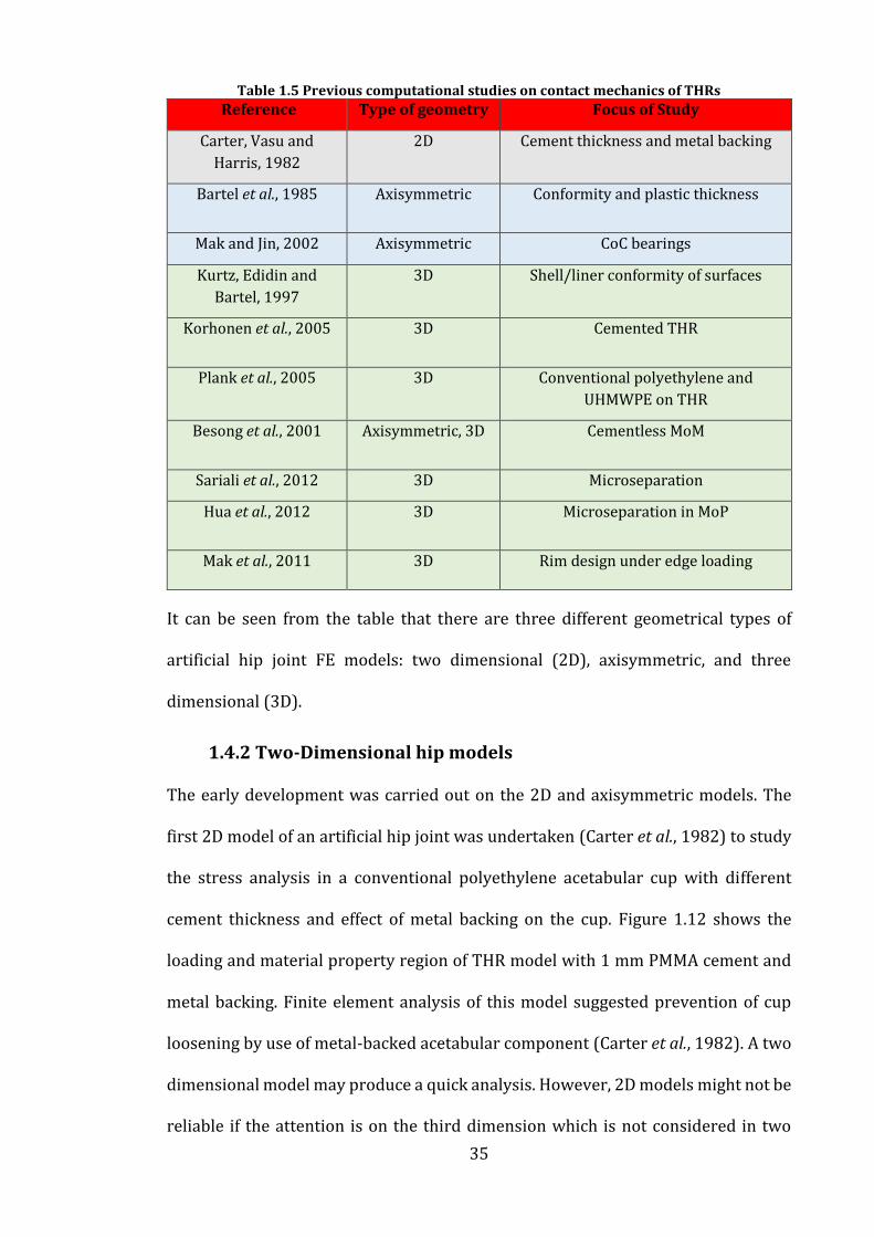
35

Table 1.5 Previous computational studies on contact mechanics of THRs

Reference Type of geometry Focus of Study

Carter, Vasu and

Harris, 1982

2D Cement thickness and metal backing

Bartel et al., 1985 Axisymmetric Conformity and plastic thickness

Mak and Jin, 2002 Axisymmetric CoC bearings

Kurtz, Edidin and

Bartel, 1997

3D Shell/liner conformity of surfaces

Korhonen et al., 2005 3D Cemented THR

Plank et al., 2005 3D Conventional polyethylene and

UHMWPE on THR

Besong et al., 2001 Axisymmetric, 3D Cementless MoM

Sariali et al., 2012 3D Microseparation

Hua et al., 2012 3D Microseparation in MoP

Mak et al., 2011 3D Rim design under edge loading

It can be seen from the table that there are three different geometrical types of

artificial hip joint FE models: two dimensional (2D), axisymmetric, and three

dimensional (3D).

1.4.2 Two-Dimensional hip models

The early development was carried out on the 2D and axisymmetric models. The

first 2D model of an artificial hip joint was undertaken (Carter et al., 1982) to study

the stress analysis in a conventional polyethylene acetabular cup with different

cement thickness and effect of metal backing on the cup. Figure 1.12 shows the

loading and material property region of THR model with 1 mm PMMA cement and

metal backing. Finite element analysis of this model suggested prevention of cup

loosening by use of metal-backed acetabular component (Carter et al., 1982). A two

dimensional model may produce a quick analysis. However, 2D models might not be

reliable if the attention is on the third dimension which is not considered in two

36

dimensional models. For example in this study, stress distribution has been

considered only on the central plane not on the inner surface of the cup. In two-

dimensional models, plane strain is assumed (i.e. the strain out of the plane is

assumed to be zero).

Figure 1.12: 2D model of THR with A) 1 mm PMMA and B) with metal backing (Carter et al., 1982)

1.4.3 Axisymmetric hip models

An axisymmetric model is basically suitable for the symmetric configuration about

an axis and it is usually used for replacing 3D model with simple configuration to

save computational resources. 2D and axisymmetric models represent high

computational efficiency and lower computational storage compare to 3D models.

Therefore, they are developed to establish initial estimation of the problem.

An axisymmetric contact model of UHMWPE acetabular cups against metallic

femoral heads (Figure 1.13) was developed to predict the contact area and stresses

in articulating surfaces under various loads. The result of this configuration was

compared to the experimental measurements and simple elasticity analysis for data

validation (Jin et al., 1999). Another axisymmetric model (Figure 1.13) was

developed by Bartel et al (1985) to study the effect of conformity and plastic

thickness on contact stresses in metal backed plastic implants (Bartel et al., 1985).

37

This study was based on linear elastic behaviour; however, polymers display elastic

and also plastic behaviours when the yield stress is exceeded.

Figure 1.13 The axisymmetric models of THR A) The axisymmetric finite element model of Jin et al (1999) B) Axisymmetric THR model of Mak and Jin (Mak and Jin, 2002) C) FE model

of metal backed plastic cup in Bartel et al (1985)

An axisymmetric finite model of CoC bearings was developed by Mak and Jin to study

contact mechanics of this type of bearing (Mak and Jin, 2002). This model included

ceramic insert and head, metallic stem, and a polyethylene backing secured in

metallic shell for fixation purposes. Figure 1.13 shows the construction of these

components. The much higher elastic modulus of the metal than the polyethylene

meant that its effect was negligible for this model. This study indicated that the

contact mechanics of the CoC THR largely depends on design parameters such as

radial clearance and ceramic insert thickness. Furthermore, it was demonstrated

that Hertz contact theory is an applicable method for validation of CoC

computational models.

If the contact analysis is carried out on axisymmetric models, the hip joint has been

implanted vertically to have XY axis as an axis of symmetry. However, in vivo, the

cup is implanted with different inclination angles with respect to the femoral

components. Thus, the actual assembly of the hip replacement in vivo is not

comparable to the axisymmetric configuration.

38

1.4.4 Three-Dimensional hip models under idealised condition

Three dimensional models of THR have been widely developed to investigate the

effect of design parameters and surgical techniques on the contact mechanics of the

articulating surfaces. The running time of the 3D THR models is longer than 2D and

axisymmetric models as more calculations are required compared the 2D and static

models. However, these models are generally more realistic output as three

dimensional effects of the kinetics and kinematics are taken into consideration in

contact mechanics studies. In fact, one previous study has showcased the difference

in the contact output of axisymmetric and 3D models of the THR (Besong et al.,

2001). The model consisted of a titanium shell, cobalt chrome femoral head and

insert with 30µm radial clearance. The model was designed to be cementless. A 3D

model was developed to consider the loading of the joint in the anatomical position.

The comparison of axisymmetric and three dimensional models suggested a

difference between the peak contact pressure in axisymmetric and 3D model of the

THR (5MPa difference in the peak value) which is caused by the anatomical loading

and axial loading in 3D model and axisymmetric model.

Three dimensional THR FE models are generally carried out on idealised conditions

and the 3D modelling of separation has only recently been introduced (Sariali et al.,

2012; Hua et al., 2014). In this section, the FE THR models under the idealised

condition are reviewed. Three dimensional THR replacements mainly focus on the

interfaces within the THR to predict the risk of fixation or contact failure. In addition,

the effect of design, positioning and the material properties are studied for

behaviour prediction. One of the studies that focuses on the interface between the

polyethylene liner and metal shell due to manufacturing tolerances or locking

mechanism of liner and shell was by Kurtz et al (1998). In this study, a three-body

contact (femoral head, polyethylene liner, and the shell) was solved for quasi-static

39

response with four sets of liner boundary conditions: no restraints, rim restraints,

equatorial restraints, and both rim and equatorial restraints. This study suggested

that in nonconformities designs, deformation of polyethylene liner within the shell

occurs to make a solid contact with the shell. This shell/liner interaction leads to

load transfer and relative motions between the shell and liner (Kurtz et al., 1998).

Korhonen et al studied the effect of the design and positioning of the THR by

focusing on how the geometry and abduction angle affected contact pressure and

area of a cemented THR (Korhonen et al., 2005). In this study, a FE analysis of two

clinically tested designs (IP and Labinus eccentric shown in Figure 1.14) and two

additional designs with cement mantle and femoral head were generated to predict

the effect of cup clearance and thickness on contact mechanics.

Figure 1.14 Clinically tested IP and Labinus (Korhonen et al., 2005)

A significant change of mechanical stresses on the acetabular cup was observed due

to geometrical design, thickness, and abduction angle of the acetabular cup in the

loading cycle. This analysis suggested that increased clearance leads to greater

contact pressure at interfaces and also that polyethylene layer thickness and contact

pressure have an inverse effect on cup-cement interface. Figure 1.15 shows

validation of contact area in the numerical model and experimentally tested IP and

Labrius cups which represented a fairly consistent result.

40

Figure 1.15 Contact area of the Labinus and IP cup under loading cycle in a) experimentally tested and b) numerical models (Korhonen et al., 2005)

The effect of the material properties and the bearing design were studied by Plank

et al (2005). The contact stresses in conventional and crosslinked UHMWPE

acetabular cups, different femoral head sizes and liner thicknesses were analysed.

This study focused on the contact stress on the acetabular cup. Therefore, the

femoral head was modelled as an analytical surface. Since the moduli of the femoral

head and the shell are significantly higher than the liner, these two components

were treated as rigid bodies. This approach has been taken forward in subsequent

studies as it saves computational running time due to reduced element numbers

(Hua et al., 2012).

Plank et al’s study suggested a lower contact stress occurred for crosslinked

UHMWPE than the conventional material in all the examined sizes (Figure 1.16). It

also indicated that the use of larger highly crosslinked UHMWPE head sizes with

3mm liner thickness resulted in lower stress than conjunction of smaller

conventional head with 3 mm liner thickness. The FE analysis also represented a

41

consistent result with experimental measurement of contact pressure by use of Fuji

film.

Figure 1.16 Maximum stress of FE models of THR using conventional and highly cross linked ULHMWPE (Plank et al., 2005)

1.4.5 Three dimensional hip models under microseparation

condition

There have been a small number of three-dimensional finite element models of THR

that studied the effect of microseparation, cup inclination angle, cup abduction

angle, and radial clearance between the femoral head and the cup on the contact

mechanics of articulating surfaces of THR (Mak and Jin, 2002; Sariali et al., 2012;

Hua et al., 2014). Mak et al THR model (Figure 1.17) consisted of alumina femoral

head and bearing insert, metal stem and shell, and polyethylene backing. An

assumption was made that fully bonded interfaces occurred between backing and

insert and also between femoral head and stem, allowing concentration on the

contact of the femoral head and bearing insert in a range of different

microseparation conditions. The radial clearance was assumed to be 0.04 mm and

thickness of the bearing as 5mm. A simple analysis was firstly followed to determine

when microseparation would lead to edge loading. Frictionless contacts were

assumed.

42

Figure 1.17 THR modelled by Mak et al with 45o cup inclination angle (Mak and Jin, 2002)

The result of this study suggested that the microseparation which is required to

cause edge loading of the THR is inversely proportional to the cup inclination angle

and proportional to the radial clearance. Furthermore, it was observed that smaller

microseparation is required in hard-on-hard bearings to cause edge loading due to

close conformity and small clearances. This study also showed that microseparation

less than 80µm does not cause edge loading. However, when the microseparation

was increased to 120µm, the contact pressure was increased significantly due to the

contact of the head with the edge of the cup. Furthermore, this study suggested that

when microseparation was increased to 250µm, the cup with the filleted edge had a

great effect on reduction of the contact pressure compared with the sharp edge.

Sariali et al (2012) attempted to determine the effect of high cup abduction angle on

contact mechanics of articulating CoC bearings with different microseparation

values. A 32mm ball with 30µm radial clearance was modelled in normal conditions

(45o abduction angle and 0o anteversion angle) and for variations of cup abduction

angle (45o to 90o). In the normal condition, it was indicated that lateral

microseparation greater than 30µm caused edge loading. However, smaller values

of microseparation caused edge loading when a larger cup abduction angle was

involved. In the condition with no microseparation, the value of contact pressure

43

increased from 66MPa under normal conditions to 137.2 MPa in 90o cup abduction

angle and up to 200MPa when 240µm lateral microseparation was obtained.

Figure 1.18 shows the increase in contact pressure in the THR as the cup abduction

angle increased. This study focused on the effect of microseparation on a specific

point during the gait cycle (swing phase when the most microseparation occurs).

However, the loading on the hip is dynamic during the gait cycle and it varies

significantly with time; the contact mechanics could be affected by this variation in

the loading.

Figure 1.18 Contact pressure analysis of the CoC THR model under 0-500 µm lateral

microseparation and 65 to 90 condition (Sariali et al., 2012)

A study on edge loading of cemented hard-on-soft bearings was carried out recently

to examine the effect of cup inclination angle on contact mechanics and cup fixation

44

of THR (Hua et al., 2012). An UHMWPE acetabular cup with a 22.2mm diameter

metallic femoral head and 0.1825mm radial clearance was modelled. Cup inclination

angles from 45o to 65o were simulated with penetration of femoral head to UHMWPE

cup ranging from 0 to 4mm. As Figure 1.19 represents, the contact pressure

increases significantly when no penetration is achieved but the contact pressure

with different non-zero penetration rates only slightly varied. This study suggested

the sensitivity of the hard-on-soft bearings to cup inclination angle changes is less

than hard-on-hard bearings (Liu et al., 2005). Furthermore, the maximum von Mises

stress in the cement mantle occurred at the cup/cement interface. Comparison of

different conditions indicated that the highest von Mises stress in the cement mantle

occurred when there is 65o inclination angle with 4mm penetration due to reduction

in the cup thickness.

Figure 1.19 Contact mechanics analysis of MoP THR in different penetration rate (Hua et al.,

2012)

The previous studies that were discussed proved that when microseparation is

combined with lateral displacement or excessive cup inclination and abduction

angle, the contact of rim of the cup and head occurs and this leads to increased

45

contact stress. A new FE model of THR was carried out to predict the effect of

different cup rim geometries on the increased stress (Mak et al., 2011). In this study,

a 28 mm diameter CoC THR with 40 µm radial clearance was modelled and

microseparation distance was selected to be between 0 and 250 µm. As Figure 1.20

shows, three different edge geometries were investigated: as new, worn, and

chamfered (rim geometry after 1 million cycle of tested product in hip simulator

under microseparation conditions). It was interesting to note that different rim

geometry affected the distance for the onset of rim contact. When edge contact

initiated, the maximum contact pressure was greater if the contact area was less.

The maximum von Mises stress (672 MPa) under 250 µm microseparation was the

greatest in the ‘as new’ geometry. When the contact area becomes greater due to rim

geometry changes, the contact pressures decrease to 425 MPa and 437 MPa in worn

and chamfered rims, respectively.

Figure 1.20 Three different geometry of cup rim in Mak et al study (Mak et al., 2011)

All of the computational studies on the contact mechanics of THR under

microseparation conditions try to replicate the conditions of a specific time frame in

a gait cycle using a static calculation at that time, such as the time period when

maximum load occurs or when the separation is at the maximum level (minimum

46

axial load). However, the gait cycle is a dynamic system and therefore the THR

experiences a varying load throughout the cycle. A simple static model may not

report accurate data from its calculations as the location of the contact will vary due

to the loading changes. Further, in these studies the position of the THR components

is estimated based on the experimental separation levels or various separation

levels were tested to the model directly. Then, contact mechanics of the bearings

were analysed when a load is applied (Sariali et al., 2012). Contact mechanics of

articulating surfaces in the hip replacement have been analysed statically when a

single load or series of load is applied to the prostheses. This means in previous

studies, specific time frames of a gait cycle have been chosen and the loading

conditions of the step were applied to the model statically. Therefore, the studies

are controlled by the force rather than the motion which drives the component.

One of the other limitations of this approach is the inability to analyse the relative

motions of components of the model during an entire gait cycle, instead using only

the simplified loading condition. Since the details of the motion between the discrete

points affect the stress state, the static models are not able to analyse the contact

mechanics with real conditions especially throughout a gait cycle due to significant

changes of dynamic load compared to static conditions (Kayabasi and Ekici, 2007).

Consequently, the conjunction of dynamic and FE model is essential to achieve more

precise understanding of contact mechanics of THR in vivo and vitro. That means a

mathematical model needs to be developed to investigate first kinematics such as

motion and contact forces throughout a gait cycle (dynamics model) and then carry

out static contact mechanics analysis such as contact pressure, stress, and

deformation of components on each step (FE model).

47

1.4.6 Coupling of dynamic and contact mechanic analysis

Development of dynamic models of the prostheses to determine joint and contact

mechanics during a dynamic loading condition is the best tool to predict the relative

motion and kinematic analysis accurately. The number of dynamic studies on the

THR are limited as the hip joint is a ball and socket geometry and the contact is

usually stable. However, the dynamic studies of THR have been developed when the

idea of edge loading and increased wear were introduced due to substantial changes

in the contact condition. The most kinematic and contact mechanic integration

analyses have been carried out on the total knee replacements (TKR). Table 1.6

summarises the number of these dynamic and contact mechanics studies that were

carried out on knee and hip replacements.

Table 1.6 previous studies on coupling of kinematic and FE methods of THR

Number Model Finite element

solver method Reference

1 2D model of TKR Implicit Reeves et al., 1998

2 2D model of non-conforming

TKR Implicit

Estupinan, Bartel

and Wright, 1998

3 3D model of TKR Explicit Godest et al., 2002

4 3D model of TKR Explicit

Halloran, Petrella

and Rullkoetter,

2005

5 3D model of TKR Explicit Baldwin et al., 2009

6 THR as a pendulum model Explicit Liu et al., 2010

7 3D model of THR Explicit Gao et al., 2015

In order to solve a dynamic finite element problem, the analysis requires

incremental load or displacement steps (ABAQUS 6.12 documentation, 2012). In

each step, several linear equations, which are represented as a system called

‘stiffness matrix’, need to be solved. There are two methods which can to solve these

and generate dynamic solutions. One of the methods calculates the state of the

incremented step from the solution of the stiffness matrix from previous step using

48

a forward Euler Method. This method is called an explicit solver. Another way to

solve the dynamic model requires the stiffness matrix of the current state of the

system, and the stiffness matrix of the incremental step. This method is called

backward Euler’s method which is implicit (ABAQUS 6.12 documentation, 2012).

Reeves et al (1998) and Estupinan et al (1998) studied the cyclic dynamic loading

effect on UHMWPE behaviour by generating 2D and idealised 2D model of TKR

implicitly. The disadvantage of using implicit solver for dynamic analysis is the long

time it takes to solve the equations. Therefore, the models are restricted to two-

dimensions and these 2D models might provide valid information about the central

plane of contact. However, the stresses and deformation of THRs in the medial-

lateral direction have not yet been investigated using this approach (Estupinan et

al., 1998; Reeves et al., 1998).

Explicit models of joint replacements, mainly total knee replacements, have been

generated to predict the kinematic and contact mechanics under dynamic loading

and avoid the problems encountered by the Reeves and Estupinan groups (Godest

et al., 2002; Halloran et al., 2005; Baldwin et al., 2009). These studies used

mechanical knee simulators for direct experimental validation. Therefore, the

boundary conditions of the models were adjusted to simulate the mechanical knee

simulator environment. In these studies, the contact force was defined to be a

function of penetration distance of master into slave surface (penalty-based

method). These dynamic studies are difficult to compare directly to previous static

ones due to different loading, boundary conditions, and different implant

geometries.

The explicit models of TKR are able to simulate the soft tissue actions which have

not been considered in implicit models. The explicit models allow ‘buckling’ of soft

49

tissue whereas implicit models would cause stability problems if buckling occurs.

Soft tissue behaviour was simulated differently in each study. Godest et al (2002)

defined two planar joints to simulate the springs in the simulator that perform as

soft tissues. Halloran et al (2005) used spring elements to constrain any internal-

external and inferior-posterior displacement. In the most recent study, the tendons

and ligaments around the knee were represented in a more complex but more

realistic way by fibre-reinforced composite material model that consist non-linear,

tension only springs embedded in a low-modulus, hyper elastic deformable 2D

quadrilateral mesh (Baldwin et al., 2009).

Godest et al (2002) studied the effect of mesh density, time steps, and coefficient

friction on AP displacement, IE rotation, and internal stresses within a single

analysis. At first, the axial force, anterior-posterior force, torque, and flexion angles

a function of gait cycle were represented based on the boundary conditions. In this

study, minor variation between the theoretical kinematic data and experimental

value was seen. The exact coefficient of friction between polyethylene and metal was

unknown. Also, the mass and the inertia of the fixtures of knee simulators were

ignored (Godest et al., 2002). In engineering, dynamic model usually involves rigid

body assumptions and rigid body analysis does not calculate internal stress and

strain of each element. Therefore, a softened contact which does not consider

internal stress was defined when the interaction occurs (Godest et al., 2002).

Halloran et al (2005) and Baldwin et al (2009) developed explicit model of Stanmore

knee simulator, Purdue knee simulator, and Kansas knee simulator to study tibio-

femoral and patella-femoral articulation using two different methods (Halloran, et

al., 2005):

1) Fully deformable model

50

2) Rigid body analysis

The rigid body model was used to analyse the kinematic data with significantly

shorter computational time. However, a softened contact capability had to be

defined to be able to study contact mechanics of the model. In both studies the

kinematic data was determined and the data were experimentally validated. In the

Halloran group’s study, the kinematic data approached a good agreement although

the same assumptions of material properties of polyethylene and same coefficient

of friction as Godest et al study were used. Both rigid body analysis and fully

deformable models gave reasonably close data (Figure 1.21). However, it should be

noted that use of softened contact also requires estimation of non-linear pressure-

overclosure relationship by material property data. A limitation of this method is

the significant central processing unit (CPU) time usage of a fully deformable

analysis.

Figure 1.21 Contact pressure contour comparison during the gait cycle for both deformable

(left) and rigid body (with softened contact) (right) analyses et al., 2005)

1.4.7 THR dynamic modelling

Liu et al (2010) tried to simulate MoM, CoC, and MoP resurfacing total hip

replacement in a simple pendulum model to study THR dynamic and contact

51

mechanics analysis of the component interaction. The THR was simulated as a ball

in socket geometry of the fulcrum and the ball was connected to a mass ball by a

massless wire (Figure 1.22). Hence, different motion angles and dynamic loading of

the mass ball simulated simple kinematic data that a hip joint experiences. This

study was carried out using coupled (using explicit model) and decoupled (using

explicit and standard) method (Liu et al., 2010).

In coupled method, both dynamic and contact mechanic analyses were carried out

in ABAQUS/explicit. However, in the decoupled method, the dynamic response was

predicted using ABAQUS/explicit and the corresponding force predicted from

explicit model was applied to the ABAQUS/standard model at different time steps

to investigate contact mechanics analysis. In the coupled method, the cup was

assumed to be a fully deformable model and femoral head was set as analytically

rigid body whereas in the decoupled method, the cup was set as analytically rigid

body for dynamic analysis. The same boundary conditions and parameters such as

elements and mesh were used for both methods.

In the Liu et al study, the contact pressure of implicit model was compared to

dynamic transient pressure of explicit model. Although both methods predicted

adequately the dynamic and contact mechanics under the conditions, the decoupled

method was more efficient in predicting THR performance. The main limitation of

this study was the difference in the dynamic response and motion angle of the

pendulum model (Figure 1.22) to the gait cycle. The pendulum model response force

and motion angle were similar to sinusoidal and cosinusoidal waveforms,

respectively. However, the gait cycle consists of various loading conditions including

swing and stance phase and its motion is more like ‘V’ shape with different

maximum and minimum values. Also, this study did not consider the effect of

52

muscle forces on the analysis. It only applied the body weight which is considered

to the hip joint during a walking cycle.

Figure 1.22 The pendulum model used in Liu et al study (Liu et al., 2010)

Three dimensional dynamic and contact mechanics modelling of the THR is still

under development and most of the studies in this area only present the

development criteria of this type of modelling and do not draw significant

conclusions. Gao et al, studied the explicit modelling of the THR under normal

walking cycle (Gao et al., 2015). In this study, the range of motion and anatomical

loading of the THR (Figure 1.23) was applied to the explicit method model to justify

the use of explicit method. The study contrasts the explicit method to the implicit

and analytical methods, and also aims to show the accuracy and efficiency of the

explicit method. Mesh sensitivity analysis and time steps were examined on the

contact pressure and sliding distance of the hip with respect to the cup. This study

shows that explicit method is a useful method to predict and capture the contact

pressure and accumulated sliding distance for THR in a gait cycle. However, this

study is limited to one set of normal walking activity and it does not recommend

that explicit modelling is a convenient method for a range of activities when the

stability is significantly less.

53

Figure 1.23 a) CAD and b) FE models of an artificial hip joint in Gao et al study (Gao et al.,

2015)

1.4.8 Wear modelling

Another type of modelling that is carried out on THRs is wear modelling. Wear

modelling has focused on wear of hard-on-soft bearings, initially made from

polyethylene (Maxian et al., 1996; Wang et al., 1998), and more recently has evolved

with the technology to model hard-on-hard bearings (Liu et al., 2008). In these wear

models, the formula for wear prediction based on sliding distance, load and the wear

factor which is assumed to be constant throughout the analysis. Other factors that

are considered in wear studies are the lubrication form and the thickness which

affects the wear directly (Mattei et al., 2011). The wear studies are used to predict

the wear scar on the bearing surfaces and the film thickness. However, the

assumption of constant wear factor does not allow a realistic wear prediction

against the experimental studies as the wear factor varies based on the load, velocity

and the loss material volume (Mattei et al., 2011).

1.5 Summary

The performance of THR devices can be affected by the quality of the tissues

surrounding the joint or the mismatch of the component centres during hip

replacement surgery. Experimental studies have shown that these factors can cause

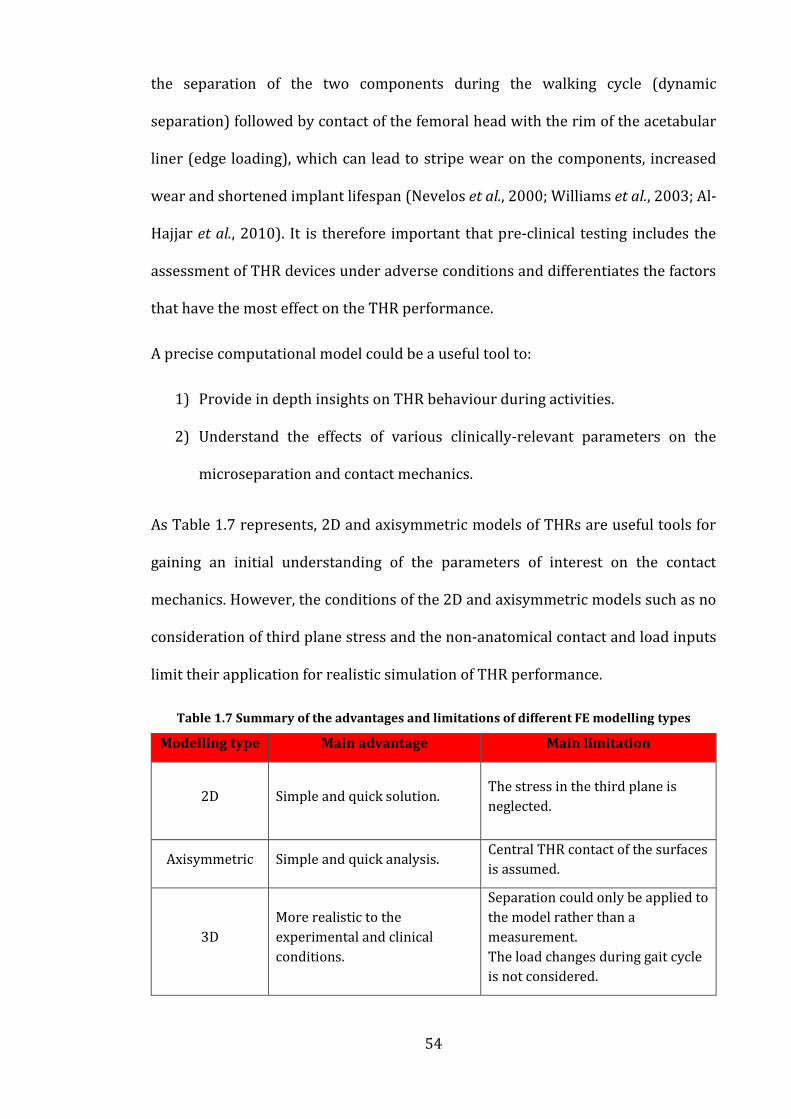
54

the separation of the two components during the walking cycle (dynamic

separation) followed by contact of the femoral head with the rim of the acetabular

liner (edge loading), which can lead to stripe wear on the components, increased

wear and shortened implant lifespan (Nevelos et al., 2000; Williams et al., 2003; Al-

Hajjar et al., 2010). It is therefore important that pre-clinical testing includes the

assessment of THR devices under adverse conditions and differentiates the factors

that have the most effect on the THR performance.

A precise computational model could be a useful tool to:

1) Provide in depth insights on THR behaviour during activities.

2) Understand the effects of various clinically-relevant parameters on the

microseparation and contact mechanics.

As Table 1.7 represents, 2D and axisymmetric models of THRs are useful tools for

gaining an initial understanding of the parameters of interest on the contact

mechanics. However, the conditions of the 2D and axisymmetric models such as no

consideration of third plane stress and the non-anatomical contact and load inputs

limit their application for realistic simulation of THR performance.

Table 1.7 Summary of the advantages and limitations of different FE modelling types

Modelling type Main advantage Main limitation

2D Simple and quick solution. The stress in the third plane is

neglected.

Axisymmetric Simple and quick analysis. Central THR contact of the surfaces

is assumed.

3D

More realistic to the

experimental and clinical

conditions.

Separation could only be applied to

the model rather than a

measurement.

The load changes during gait cycle

is not considered.

55

The THR undergoes a range of loading in an activity. However, previous

computational studies of the THR have modelled the loading cycles as a series of

static frames that do not take account of the dynamic conditions. Previous

computational studies of separation have mostly focused on the effect of

microseparation on the contact mechanics of the 3D THR at a specific time of

walking cycle (Hua et al., 2012). There are no computational studies that focus on

the effect of individual parameters on the separation and contact mechanics of THR

under dynamic loading.

The idea of the integrated dynamic and contact mechanic computational model of

THR has been recently introduced and there have been only limited initial studies

on this area. However, the previous studies mostly report the sensitivity of the

models to certain conditions and none of the previous studies incorporating

dynamics and contact mechanics have focused on the separation effects.

1.6 Aims and objective

The ultimate aim of this project was to develop a preclinical computational tool in

order to examine the effect of clinically-relevant parameters on the separation and

contact mechanics of hard-on-soft THRs as the recent analysis have shown that

hard-on-soft bearings are the most common THRs that have been used in England

(National Joint Registry, 2016).

This developed model can have variety of applications in industrial, experimental

and clinical perspectives. As this model studies the direct effect of input parameters

on the separation and contact mechanics, the source of THR weakness in adverse

conditions can be detected and consequently, the design, material combinations and

the positioning of the bearings can be optimized to reach higher tolerance to edge

loading. Moreover, the durability of THR can be potentially prolonged for more

56

active and young patients when the component is less affected by wear due to the

separation and edge loading. Although, in vitro testing has been carried out under

adverse conditions to study the wear rate of the THR, this is the most applicable

method to analyse the hip implants in a clinical and experimental environment that

is cost and time effective. This model could be used as a tool to analyse the effect of

wide range of parameters on the outcome and the most crucial parameters can be

tested in vitro.

To achieve this aim, a finite element model of the THR was developed that could

simulate the dynamic motion during a gait cycle and predict the THR separation and

contact mechanics. The developed computational model replicates one station of an

existing hip simulator so that comparisons could be made for validation purposes.

The following objectives were set to achieve the aim of the project (Figure 1.24):

Develop an explicit dynamic FE model of a simplified THR under concentric

conditions that replicates one station of Leeds II hip simulator and examine

the effect of computational modelling choices on the outputs (This work is

presented in Chapter 2).

Develop an explicit dynamic FE model of a Pinnacle ceramic-on-polyethylene

(DePuy Synthes) THR under adverse conditions including a mechanism for

separation during swing phase (This work is presented in Chapter 3).

Study the effects of varying clinically relevant parameters, namely, the

translational mismatch level, the rotational variation and the swing phase

load on the dynamics of the THR. (This parametric sweep is presented in

Chapter 4).

57

Validate the computational model output against existing experimental data

by comparing the in vitro and in silico separation (This work is presented in

Chapter 4)

Examine the effect of translational mismatch level, rotational variation and

swing phase load on the THR contact mechanics including the contact

pressure and stress components that cannot be measured experimentally

(These additional output of the parametric sweep is presented in Chapter 5).

58

Figure 1.24 The flowchart and order of the chapters with a brief description of the chapters focus

59

Chapter 2 Development of the explicit model under

concentric loading conditions

2.1 Introduction

The foremost aim of this project was to develop a computational model of a total hip

replacement (THR) to study the effect of parameters, such as surgical

malpositioning, on the contact mechanics of THR during walking. Subsequently,

validation of the model with existing in vivo or in vitro studies is required in order

to examine its reliability and accuracy. Therefore, for validation purposes, the

computational model was established to replicate the Leeds II hip simulator. This

simulator has the capability to test the effect of adverse conditions on the

biomechanical and wear behaviour of THR.

To achieve a representative three-dimensional model of the Leeds II hip simulator,

the features of the experimental set up need to be implemented within the model as

accurately as possible. If the model is simplified to the most basic conditions, the

effect of each parameter can be studied separately and gradually increase the

complexity of the model. This method would allow the determination of which

parameters have the most and the least effect on the analysis – i.e. the sensitivity of

the model. Therefore, more engineering effort can be spent on the factors to which

the model is most sensitive and less consideration to the factors which have only

negligible effect on the results. The model was developed gradually by investigating

a standard (concentric) scenario as well as an adverse condition scenarios. The

model development under standard conditions provide information on the

fundamental computing factors and provides a benchmark with which to compare

results from further analyses. The effect of adverse conditions on the overall

computational model behaviour can be observed when adverse conditions are

60

applied in the further steps. These adverse effects can be studied individually, or

built into a singular model to study their interdependencies.

This chapter focuses on the initial development of the ceramic-on-polyethylene THR

model under standard conditions. In this chapter the overall replication of the Leeds

II experimental set up such as components movement and loading is described. To

be able to achieve a computational model that produces reliable contact mechanics

analysis, the components movements and axial loading should be applied to the

model correctly as the contact mechanics are directly affected by the loading and the

kinematics. Furthermore, the effect of computational parameters, namely mesh

sensitivity analysis, contact algorithms, and loading methods, on the model outputs

are is considered.

2.2 Experimental setup of Leeds II hip simulator

The Leeds II simulator is a physiological and anatomical hip joint simulator that has

been used to test the Pinnacle THR under standard and adverse conditions (Al-

Hajjar et al., 2010), specifically translational mismatch level, cup inclination

variation and tissue laxity. This simulator consists of six identical stations, in each

station of which, there is a stem holder that fixes the femoral stem which carries the

femoral head on top (Figure 2.1). The cup unit is located at a certain inclination angle

above the head and carries the metal shell and the acetabular cup in such a way that

the surface of the acetabular cup articulates with the femoral head. There is a 10°

difference between the clinical and simulator inclinational angle due to the 10°

difference in the clinical and experimental loading angle (Williams et al., 2003). An

axial load is applied to the model via a load cell that is located on top of the cup

holder. There is also a spring attached between the wall of each station and the cup

unit horizontally to allow different levels of translational force to be applied. Each

61

station is filled with a lubricant (bovine serum) to replicate the lubrication of THR

in vivo and minimise the coefficient of friction between the components.

Figure 2.1 Schematic of the experimental set up of Leeds II hip simulator with rotation and loading locations indications

In the simulator, the THR components are taken through specific movements to

simulate the walking pattern of the patient’s right hip. During the gait cycle, the cup

is driven to move medial-laterally and rotate internal-externally. However, the cup

is free to translate anterior-posteriorly and superior-inferiorly. Moreover, the

flexion-extension of the hip is implied through the femoral head. There is an axial

load applied through the cup to the hip joint on each station. Figure 2.2 represents

the Paul twin peak cycle load (Paul, 1976) as per ISO 14242-1 (2002) that is a

representative of the load which the hip undergoes during walking. The load cell is

located on top of the cup unit and it records the load applied vertically downwards

on the cup. When no axial load is applied to the model, the horizontal spring

separates the cup and the head and applies a translational mismatch level. Maximum

62

load in the stance phase causes maximum compression of the spring level, whereas

low load during swing phase results in partial compression of the spring and contact

of the head with the lateral edge of the cup.

Figure 2.2 Example of Paul cycle loading in Leeds II hip simulator (Paul, 1976; Al-Hajjar et al., 2013)

2.3 Design of numerical study

As dynamic modelling of the artificial hip joint is novel, the main aim of this analysis

was to gain a fundamental understanding of dynamic analysis within the explicit

ABAQUS software package (Version 6.14, Dassault Systèmes Simulia Corp.,

Providence, United States). The main outcome of this specific study was to

investigate the level of sensitivity of contact mechanics analyses to the

computational factors that can directly influence the contact mechanics of the

model.

If the initial development includes the full complex geometry, a wide range of

movements of the components and a holistic loading profile as well as parameters

within modelling such as mesh density, contact algorithms and loading and

boundary conditions, the complexity of the model will be increased considerably.

0

500

1000

1500

2000

2500

3000

3500

0 10 20 30 40 50 60 70 80 90 100

Load

(N

)

Time (ms)

63

Therefore, if all the parameters are analysed at the same time, fault finding and

diagnostics during the model development would be considerably more challenging.

The time taken and computational cost to solve the model is increased with model

complexity, and there is no guarantee at the early stages that the engineering effort

is directed toward the most significant factors.

A representative dynamic model of the Leeds II hip simulator was therefore

analysed for the initial results. This model consisted of simple geometry and loading

with no motion, thereby eliminating the meshing and movement complexity effect

for preliminary examination of the model behaviour. The results presented in this

chapter are for this simple model.

Incremental development of the model in terms of loading, motion and geometry

was carried out, verifying the computational results at each stage by comparison

with the experimental results from the simulator.

The meshing configuration plays an important role in the reliability and efficiency

of the contact mechanics output. Therefore, one of the parameters that this study

focuses on is the mesh sensitivity in terms of mesh density and element ratio of the

contact surfaces. Another factor that is taken into consideration is the contact

algorithms between the contact surfaces. There are numbers of numerical contact

solutions for contact mechanics analysis that are described later in this chapter.

Also, due to dynamic modelling dependency to the running time, the effects of

loading and preloading on the contact mechanics analysis are studied. Several

output parameters, namely contact pressure and contact area, that are good

representatives of the contact conditions are analysed. Furthermore, to understand

any difference between the input and output forces, the reaction forces of the

64

analyses are investigated. Finally, a static loading analysis of the model with the

same configuration was carried out to verify the outcome of the dynamic model.

2.4 Methods of Numerical Analysis

This project ultimately focussed on the contact mechanics of the adverse loading

scenario. The numerical contact calculation is directly affected by the applied

contact algorithm. Hence, it is important to select a contact algorithm that

represents the most robust outcome with respect to the model application. The

finite element analyses were solved using ABAQUS software (Version 6.14, Dassault

Systèmes Simulia Corp., Providence, United States). In this section the types of

dynamic solving processors and contact algorithms available in ABAQUS are

defined.

2.4.1 Dynamic solving processors

ABAQUS provides two types of dynamic stress-displacement solving processors;

Implicit and Explicit (ABAQUS 6.14 documentation version 2014). Figure 2.3

represents the difference in the explicit and implicit approaches.

The implicit solver is a direct integration dynamic procedure that integrates the

equations of the motion. In order to solve the model using the implicit solver,

inversion of the stiffness matrix (k) and stating a set of nonlinear equilibrium

equations are required at each time increment. Implicit solver uses equilibrium

equations to solve for time t+Δt using state data at both t and t+Δt. The size of the

stiffness matrix which depends on the degrees of freedom of the model, determines

the computational time and cost of the analysis as it must be inverted at each

iteration.

65

Figure 2.3 The difference in explicit and implicit approaches of output calculation

An explicit solver is a central-difference method that calculates the displacements

and velocities at the beginning of each time increment. The explicit approach

requires inversion of the lumped mass matrix instead of the stiffness matrix as in

implicit. The explicit approach solves for time t+ Δt using the state at t only. Since

the explicit solver does not require to solve a set of equilibrium equations, the

computations are less expensive than for the implicit solver. However, due to the

nature of the explicit solver, the stability of the model for an optimum solution is

strongly dependent on the time increments. Therefore, to achieve the required

stability in the explicit solver, the time increments are considerably shorter. The

time increment for stability in the explicit solver is conditional on the time that an

elastic stress wave takes to cross the smallest element in the model. Hence, if there

are very small elements in the model, the stable time increments become very short.

However, there are methods such as mass scaling that artificially increases the mass

66

of certain elements stability, to reduce the wave speed and as a result, increase the

overall stable time increments. The advantages and disadvantages of each method

is presented in Table 2.1.

The model stability is not a concern in an implicit solver as equilibrium equations

are an essential calculation of this solver. Moreover, a number of iterations can

happen within one time step to reach a solution in an implicit solver whereas the

explicit solver only calculates the solution for each time step once. If the explicit

solver is suitable for the required application, the explicit solver could provide the

less expensive and time consuming compared with the implicit method.

Table 2.1 Comparison of advantages and disadvantages of implicit and explicit approaches in ABAQUS

Method Advantages Disadvantages

Implicit

*Equilibrium equations used

*Stability independent of time

increment

*Reconstructing the stiffness matrix

at each increment

*Iteration required within time

increment to reach a solution

Explicit

*Updating the stiffness matrix at

each increment

*Computationally cheaper

*Lower running time

*Less stable

*Very small time increments

required for stability

2.4.2 Contact algorithms

ABAQUS/Explicit provides two types of algorithm to define contact and interaction

problems: general contact algorithm and the contact pair algorithm. Contact pair

defines the possibility of contact between two defined surfaces only whereas the

general contact introduces the pairing of contact between all of the surfaces.

The ‘contact pair’ algorithm has more restrictions on the type of surfaces which are

in contact compared to the ‘general contact’. In the contact pair, the surfaces must

67

be specified between the two surfaces. Therefore, the general contact algorithm is

more convenient in model with many objects with different undefined contacts. The

general contact algorithm uses only one method to minimise the overlap of surface

nodes in contact while the contact pair algorithm provides an extra option to

prevent the penetration of the contact surface elements. Since only the contact

between two surfaces, the head and the inner surface of the cup, was of the interest

in this project, it was logical to use the ‘contact pair’ algorithm.

2.4.1.1 Contact constraint methods

When the kinematic state of the model changes where the contact takes place,

penetration of the nodes lying on the contact surfaces occurs. The contact constraint

prevents excessive penetration of these contact surface nodes. The contact pair

algorithm can use one of two contact methods, namely the penalty or kinematic

methods, to enforce contact constraints between the surfaces. The application of the

contact constraint depends on the type of contact.

One of the parameters that affects the calculation of contact constraints is the

relationship between the two contact surfaces. The contact surfaces in ABAQUS are

defined based on the stiffness of the surface due to their assigned material

properties. The stiffer surface - usually based on relative Young’s modulus value -

defined as the master surface and less stiff surface as the slave surface. If there is a

pure master-slave surface relationship, then the constraint is always applied to the

slave surface. This means that the only penetration which is allowed is that of the

master surface into the slave surface. No node on the slave surface can penetrate

the master surface (Figure 2.4). If there is a balanced master-slave relationship, each

surface would be considered in turn as slave surface and again as master surface.

Hence, the contact constraint will be the weighted average of both calculations in

68

the form of constraint reaction forces. Balanced master-slave contact results in

better contact constraint enforcement because of better performance in minimising

the penetration between surfaces. Therefore, the balanced master-slave

relationship was used in this study.

Figure 2.4 Master-slave surfaces contact constraint in ABAQUS that represent the penetration and gap between the master and slave surface

Penalty and kinematic contact constraints are the available algorithms for

penetration prevention in ABAQUS explicit models. The penalty algorithm considers

the current configuration of surfaces nodes and behaves like a spring to return the

penetrated node to the contact surface. In a pure master-slave surface relationship,

the penalty contact algorithm identifies the slave nodes which penetrate the master

surface and applies an equal and opposite forces that are functions of penetration

distance to the penetrated slave nodes and the nodes of the master surface being

penetrated. The penalty algorithm with a balanced master-slave surface

relationship determines the contact forces to oppose penetration using the same

approach. However, one set of contact forces are calculated by assuming one surface

as a master surface, and the other contact force is calculated using the same surface

69

as the slave surface. The balanced master-slave surface relationship considers the

weighted average value of these contact forces to be applied to the model.

The kinematic contact constraint method uses a kinematic predictor to enforce

contact constraint strictly whereas the penalty method applies weaker enforcement

of contact constraints. In a kinematic contact algorithm with a pure master-slave

relationship, the contact conditions are firstly ignored to estimate the predicted

kinematic state of the model. The level of penetration of the slave nodes into master

surface, the mass associated with the corresponding node and the time increment

are then used to calculate the resisting force to minimise penetration. In case of

element face formation of the master surface, the resisting forces and mass of the

contact slave nodes are distributed over the master surface nodes to calculate the

inertial mass of the contact surfaces and acceleration correction of the master

surface nodes. Then acceleration correction for the master surface nodes is applied

to determine the acceleration correction of slave surface nodes using the predicted

penetration of the nodes and the time increment. These corrected accelerations are

required to achieve a contact configuration that can be used to enforce the

constraints. The balanced master-slave surface relationship with the kinematic

contact algorithm also use the same method. However, the procedure is followed

twice because each surface is considered once as a slave surface and another time

as a master surface. Hence, the corrected value applied by ABAQUS/Explicit is the

weighted average of the two cases.

The ideal contact algorithm to choose depends on the application of the model and

types of bodies in contact. There are limits to the type of surfaces which can be used

with the kinematic contact algorithm. For example, rigid surfaces are not allowed to

be considered as slave surfaces in the kinematic algorithm whereas penalty

70

algorithm does not restrict rigid surfaces to be mated and therefore allows

modelling of contacts between rigid surfaces. Another difference between two

algorithms is that the kinematic contact does not affect the critical time increment

for stability; however the critical time increment could become affected if the

penalty contact is used. The penalty contact algorithm includes a “spring” stiffness

which relates the contact forces to the penetration depth. The stiffness of the contact

can be changed to minimise the effect of this algorithm on the time increment.

2.5 Development of the Numerical Model

This section presents the methodology for the first stage of the explicit dynamic

model development. The analyses that were carried out in this section are separated

into three different studies. The common aspects to all models, namely geometry,

material properties and boundary conditions in this part of the study are defined in

this section. Also, the specifications of the three preliminary studies, mesh

sensitivity, contact method effect and loading conditions, on the contact mechanics

of the model are described.

2.5.1 Materials

As mentioned above, the model is intended to be simplified to minimise the effect of

any geometries complexity on the contact mechanics analysis. Therefore, the

preliminary model is composed simply of the femoral head, acetabular cup and the

cup holder. The femoral head and acetabular cup are simplified to a simple ball and

socket geometry. The details of the real Pinnacle femoral head and cup are not

considered at this stage of the model development. The cup unit is modelled as a half

sphere which has the same mass as the actual cup unit. Figure 2.5 presents the head,

the cup and the cup unit assembled vertically on top of each other.

71

Figure 2.5 Assembly of the simplified model. The crosses locate the boundary conditions on the head and the cup holder.

A ‘tie’ constraint was generated between the inner surface of the cup unit and the

outer surface of the cup to prevent all relative movement between the surfaces. To

simulate the experimental movements of the components, the head was fully fixed

at a point on its lower surface as it is a rigid body. An additional boundary condition

preventing rotation in any direction was applied to a point at the top of the rigid cup

unit. However, the cup was able to translate in any direction. Also, the loading profile

was applied to the cup unit through the same point which the boundary condition

of the cup unit was applied.

The dimensions and representative material properties of the components are

presented in Table 2.2. The ball and cup radii were chosen to create a radial

clearance of 0.25mm. Under the initial conditions, before any load was applied, the

ball surface was assumed to be coincident with the cup surface at its centre for

contact simplifications. However, the ball and the socket were modelled as

deformable bodies. However, the cup unit was considered to be a rigid body. It

should be noted that the density of the materials are scaled to lengthen the time

increment for stability and reduce the running time for these initial studies. The real

densities that will be applied to the model are described in later chapters.

72

Table 2.2 Geometric and material properties of simplified computational model components

Part Material

Young’s

modulus

(MPa)

Poisson’s

ratio

Scaled

Density

(kg/mm3)

Outer

radius

(mm)

Inner

radius

(mm)

Ball Ceramic 350,000 0.21 4.37x10-6 18 -

Cup Polyethylene 1,000 0.46 9.23x10-7 24.25 18.25

Cup

unit Rigid - - 8.5x10-6 27.25 24.25

The analyses that were carried out in the first stage of the development are

presented briefly in Table 2.3. This table shows the parameters that were varied in

the studies. The inputs which were constant in all cases namely geometry, material

properties and boundary conditions have been excluded from this table. Detailed

descriptions of the studies are given in each section that follows. The name of the

‘case’ of each study refers to the element size in cup divided by the element size in

head.

In the analyses that are described in this chapter, several output factors were

examined:

1. Contact area: Contact area is a good representative of the contact condition

in different cases. The contact area can be compared at all the time points

through simple observation of the predicted contact area plots. Also, the level

of numerical noise in the contact mechanics can be observed by analysing the

contact area data. The contact area is expected to follow clearly the loading

changes. Therefore, the contact area is predicted to increase from zero to the

peak value and then becomes constant at this peak value.

2. Contact pressure: The contact pressure plots on the contact surfaces provide

greater visualisation of the pressure distribution in various meshing

configurations. Therefore, this shows how the contact conditions can be

affected by the element size and contact surfaces meshing ratio. As the

73

contact surfaces are symmetrical spheres, the contact pressure distribution

is predicted to be circular surrounding the centre of the inner cup surface.

Table 2.3 Full list of modelling cases of stage 1 of development namely, meshing ratio between the head and the cup inner surface, loading amplitude and contact constraint

algorithm

Study Case

Mesh Loading

Contact

constraint

algorithm

Global

Element

size (mm)

Total

number

of

elements

Pattern Interpolation

Head Cup

I Case 2:3 2 3 6,220 Simplified Smooth step Kinematic

I Case

1.5:1.5 1.5 1.5 18,997 Simplified Smooth step Kinematic


I Case 1:1.5 1 1.5 47,021 Simplified Smooth step Kinematic


I Case

1:0.75 1 0.75 96,726 Simplified Smooth step Kinematic

I Case


I Case


II Contact A 1 1 61,205 Simplified Smooth step Penalty

II Contact B 1 1 61,205 Simplified Smooth step Kinematic

III Preloading

A 1 1 61,205 Preloading Tabular Kinematic

III Preloading

B 1 1 61,205 Preloading Smooth step Kinematic

III Paul Cycle 1 1 61,205 Paul cycle Tabular Kinematic

74

2.5.2 Study I: mesh sensitivity analysis

In this study, mesh sensitivity analysis was carried out on the model to achieve the

best possible level of precision with respect to computer resources. A simplified

loading profile was applied vertically downwards to the cup unit to determine the

right mesh density and meshing ratio between the contact surfaces. The model was

loaded up to 3kN in 0.1 seconds and the constant load of 3kN was then applied to

the model for 0.4 seconds (Figure 2.6).

Figure 2.6 Loading condition of the study I versus time

The load variation from 0 to 3kN was defined to follow an automatic smooth ramp

up (or down) of load from one amplitude value to another using a smooth step

function. The amplitude (𝑎) between two consecutive points is derived from the

equation (ABAQUS 6.12 Documentation, 2012):

𝑎 = 𝐴𝑖 + (𝐴𝑖+1)𝜉3(10 − 15𝜉 + 6𝜉2) 𝑓𝑜𝑟 𝑡𝑖 ≤ 𝑡 ≤ 𝑡𝑖+1

Where 𝜉 =(𝑡 − 𝑡𝑖)

(𝑡𝑖+1 − 𝑡𝑖)

This can be presented graphically as in Figure 2.7.

0

500

1000

1500

2000

2500

3000

3500

0 0.1 0.2 0.3 0.4 0.5

Load

(N

)

Time (s)

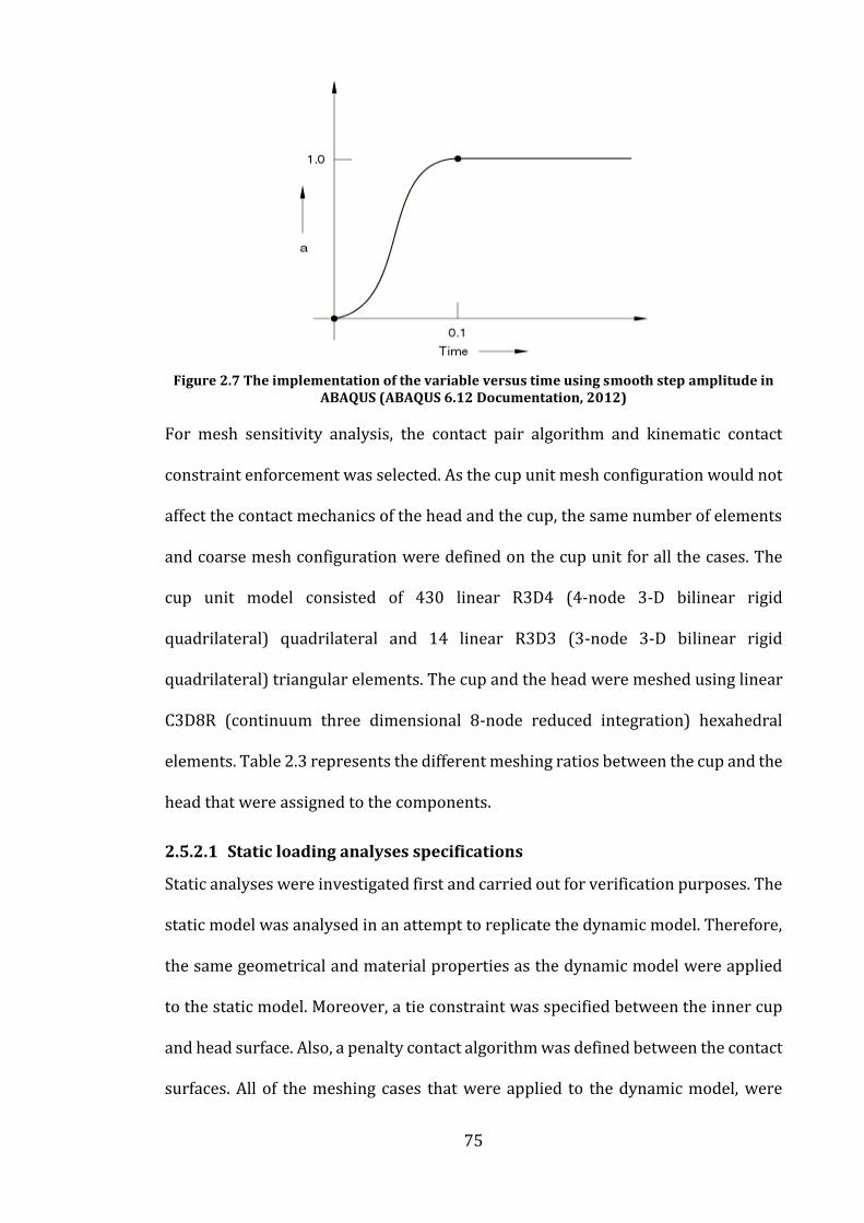
75

Figure 2.7 The implementation of the variable versus time using smooth step amplitude in ABAQUS (ABAQUS 6.12 Documentation, 2012)

For mesh sensitivity analysis, the contact pair algorithm and kinematic contact

constraint enforcement was selected. As the cup unit mesh configuration would not

affect the contact mechanics of the head and the cup, the same number of elements

and coarse mesh configuration were defined on the cup unit for all the cases. The

cup unit model consisted of 430 linear R3D4 (4-node 3-D bilinear rigid

quadrilateral) quadrilateral and 14 linear R3D3 (3-node 3-D bilinear rigid

quadrilateral) triangular elements. The cup and the head were meshed using linear

C3D8R (continuum three dimensional 8-node reduced integration) hexahedral

elements. Table 2.3 represents the different meshing ratios between the cup and the

head that were assigned to the components.

2.5.2.1 Static loading analyses specifications

Static analyses were investigated first and carried out for verification purposes. The

static model was analysed in an attempt to replicate the dynamic model. Therefore,

the same geometrical and material properties as the dynamic model were applied

to the static model. Moreover, a tie constraint was specified between the inner cup

and head surface. Also, a penalty contact algorithm was defined between the contact

surfaces. All of the meshing cases that were applied to the dynamic model, were

76

tested on the static model. No translation or rotation of the head was allowed.

However, movement of the cup unit was restricted to vertical translation only. When

translation in more axes was applied, the static model did not converge due to

stability reasons. A static load up to 3kN was applied through the cup unit.

2.5.3 Study II: Contact methods

In this study, the effect of different contact constraint algorithms was investigated.

As described above, there are two types of contact constraint enforcement that are

available in ABAQUS/explicit. To understand the effect of these contact constraints

on the contact mechanics and numerical noise, both contact constraints were tested

on the contact surfaces.

Similar assumptions of boundary conditions, loading conditions and contact

methods as in study I are conducted in this analysis. The analysis was carried out on

the best meshing configuration from the mesh sensitivity analysis (study I). The

balanced master-slave relationship was chosen for these analyses. The following

contact algorithms with contact constraint enforcements were applied to the model:

1. Contact pair algorithm with penalty contact constraint

2. Contact pair algorithm with kinematic contact constraint

2.5.4 Study III: Loading

A study was carried out to determine the effect of preloading on the initial oscillation

of the contact areas of the analysis. This study also demonstrated how this method

is applicable for Paul cycle loading. All of these analyses were carried on the same

meshing configuration and boundary condition as for study II. The considered

loading conditions are:

Preloading (Table 2.4): a magnitude of 1N was applied to the model through the

cup unit vertically downwards in 0.1 seconds using tabular (linear relationship of

77

amplitude between the consecutive points) and smooth step amplitude. Then, a

constant load of 1N for 0.2 seconds was applied following increase load of up to 3kN

in 0.1 seconds.

Table 2.4 The loading conditions of the preloading study at the specific time points (study III)

Time (s) Load (N)

0 0

0.1 1

0.2 1

0.3 3000

Paul Cycle loading: To understand the effect of the Paul walking cycle on numerical

noise and contact mechanics, the loading data exported from one station of the

Leeds II hip simulator (Figure 2.8) was applied to the model using tabular amplitude

data. There were 68 data points that represented the stance phase loading of the

Paul cycle (Paul, 1976; Al-Hajjar et al., 2013). However, two data points were

defined for the loading during the swing phase as the load during the swing phase

was constant at the load level of 300N. Also, a 5ms step was applied at the beginning

of the loading cycle to increase the load from 0 to the initial point of the Paul cycle.

0

500

1000

1500

2000

2500

3000

3500

0 20 40 60 80 100

Load

(N

)

Time (ms)

78

Figure 2.8 Paul cycle loading. The graph represents the twin peak load that is applied to the Leeds II hip simulator axially.

2.6 Results of concentric loading condition

This section presents all the results from the preliminary analyses defined

previously.

2.6.1 Study I: Mesh sensitivity analysis

ABAQUS Explicit provides two sets of contact area plots which presents the contact

area on each of the surfaces where the contact occurs. As Figure 2.9 shows, the

contact area on the head seems to increase in all the plots as the load is increased

(from 0 up to 0.1s). Furthermore, the contact area on the head undergoes a level of

oscillation as the load is constant. However, the oscillations are damped as time

progresses, and eventually the constant contact area reaches a steady state. As the

number of elements increase, the contact area tends to decrease. However, the

contact area is more sensitive to changes in the meshing ratio between the surfaces.

The contact area during the constant load phase varied between approximately

310mm2 to 360 mm2 when the same element size on the head and cup surfaces was

used. Figure 2.9 shows that there is only a slight difference in contact area when the

same meshing ratio on both surfaces was applied (plot 1.5:1.5, 1:1 and 0.75:0.75).

However, when the meshing ratio on the cup to the head element size has a double

ratio (plot 2:3, 1:2 and 0.75:1.5), the changes in the contact area are extensive

ranging from 180 mm2 to 510 mm2.

79

Figure 2.9 Contact area on the head, for different mesh resolution combinations. Each plot represents each meshing ratio condition that was carried out

Figure 2.10 demonstrates that the contact area on the cup follows almost the same

trend as the contact area on the head. It can be seen that the contact area increases

to the maximum level when the load is ramped up to the maximum value. Then, a

constant contact area was achieved when the load is held constant. Throughout the

analysis there was a constant numerical noise. The level of noise was highest when

the initial load was applied, and reduces as the model reaches a steady state. Plots

1:2 and 0.75:1.5 which are when the head that has half the element size of the cup,

produced the highest values of contact area when the load is constant (ranging from

410 mm2 to up to 910 mm2). As the difference between the element size on the

bearings decreases, the difference between the contact areas of the different cases

decreased as well. The highest number of elements with the same meshing ratio

(plot 0.75:0.75) resulted in the lowest values of the contact area. A comparison of

plot 0.75:0.75 with other plots that have the same meshing ratio (1.5:1.5 and 1:1)

indicates that the contact area of the plots are not affected substantially by using a

0

100

200

300

400

500

600

0.00 0.05 0.10 0.30 0.50

Co

nta

ct a

rea

(mm

2 )

Time (s)

02:03 1.5:1.5 01:02 01:01.5

01:01 01:0.75 0.75:1.5 0.75:0.75

80

greater number of elements (contact areas range between 340 mm2 to 400 mm2

when the load is constant).

Figure 2.10 Contact area on the cup inner surface for different mesh resolution combinations under standard condition

Figure 2.11 illustrates the differences between the contact area generated on the

head and the cup when various meshing ratios were applied. Different element size

on the contact surfaces can affect the contact area. For example, mesh configuration

0.75:1.5 which has 0.75 (head) to 1.5 (cup) element size results in a large difference

between the contact area produced on the contact surfaces of this mesh

configuration. However, if the element size on the two surfaces is similar or

minimally different, the contact area on the two surfaces is also closer to each other.

Moreover, this comparison indicates that there is a linear contact area change

during the ramp up load step in the analysis with the same element size on the

contact surfaces (1.5:1.5, 1:1 and 0.75:0.75). However, a meshing ratio of 0.75:1.5

affects the contact area variation at the load ramp up step and produces a less

consistent contact area on the head and the cup.

0

100

200

300

400

500

600

700

800

900

0.00 0.05 0.10 0.30 0.50

Co

nta

ct a

rea

(mm

2)

Time (s)

02:03 1.5:1.5 01:02 01:01.501:01 01:0.75 0.75:1.5 0.75:0.75

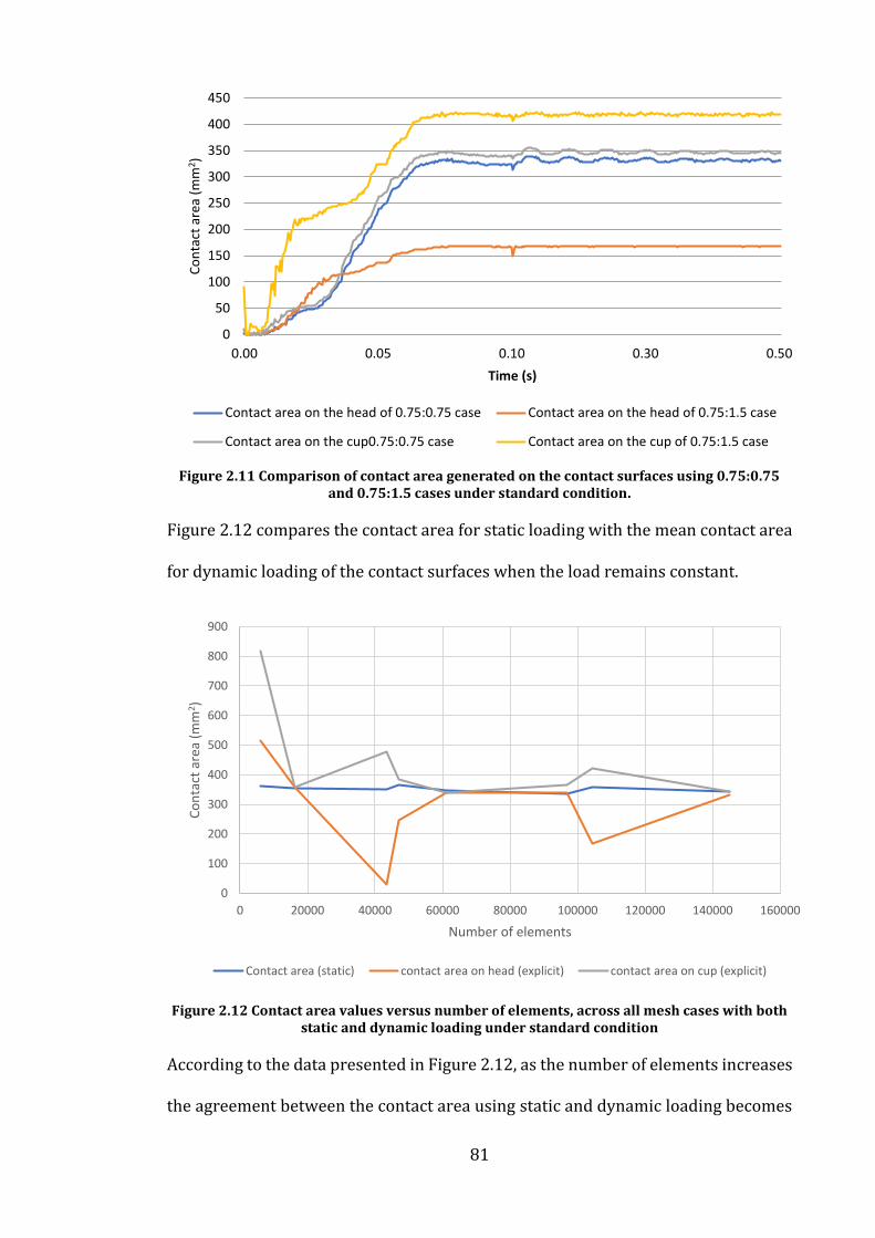
81

Figure 2.11 Comparison of contact area generated on the contact surfaces using 0.75:0.75

and 0.75:1.5 cases under standard condition.

Figure 2.12 compares the contact area for static loading with the mean contact area

for dynamic loading of the contact surfaces when the load remains constant.

Figure 2.12 Contact area values versus number of elements, across all mesh cases with both static and dynamic loading under standard condition

According to the data presented in Figure 2.12, as the number of elements increases

the agreement between the contact area using static and dynamic loading becomes

0

50

100

150

200

250

300

350

400

450

0.00 0.05 0.10 0.30 0.50

Co

nta

ct a

rea

(mm

2 )

Time (s)

Contact area on the head of 0.75:0.75 case Contact area on the head of 0.75:1.5 case

Contact area on the cup0.75:0.75 case Contact area on the cup of 0.75:1.5 case

0

100

200

300

400

500

600

700

800

900

0 20000 40000 60000 80000 100000 120000 140000 160000

Co

nta

ct a

rea

(mm

2)

Number of elements

Contact area (static) contact area on head (explicit) contact area on cup (explicit)

82

better with less than 1% disagreement, except when 104,445 elements were used.

This meshing configuration consists of the element sizes of 2mm on head and of

1mm on cup. It was illustrated previously that the 2:1 meshing ratio causes a large

difference between the contact area on the head and the cup. However, there is still

a good agreement between the contact area produced on the head using dynamic

loading and static loading are for this mesh configuration. Although finer meshing

leads to a better agreement the contact area using static and dynamic analysis, the

agreement between the contact areas depends mainly on the meshing ratio of the

contact surfaces as the cases with the same meshing ratio have better agreements.

One of the other criteria for selecting the best mesh configuration is the distribution

of the contact pressure on the surfaces. Since the contact is occurring in the centre

of the cup surface (about which the contact is symmetric), the ideal contact pressure

should be distributed symmetrically along the surface. The contact pressure is

expected to be circular due to the shape of the contact faces which are both

spherical. The pressure distributions of the contact surfaces in the last step of the

analysis for each meshing configuration are presented in Table 2.5. The contact

pressure distribution depends on the element size ratio of the contact surfaces. For

example, the element size ratio of 1.5 (cup) to 1 (head) causes the contact pressure

distribution on the surface to be more four-sided than circular (Case 2:3 and 1:1.5)

whereas a circular contact patch is predicted due to the conforming where of the

spherical contact surfaces. According to this table, a circular pressure distribution is

achieved on the cup surface when the element size on the head is half the cup

element size (mesh configuration 1:2 and 0.75:1.5). However, the majority of the

contact area appears under the maximum pressure (red area of the pressure

distribution). Furthermore, the contact pressure on the head surface does not seem

83

to be continuous for these cases which could be due to different element sizes on the

contact surfaces.

When the same element size is applied to both surfaces (highlighted columns on

Table 2.5), the contact pressure on the cup surface gradually increases from the

boundaries to the centre. Although the contact pressure is not as circular as the one

with different element sizes the contours of contact pressure appeared to be more

reasonable. The contact pressure on the head in the same meshing ratio cases

(1.5:1.5, 1:1 and 0.75:0.75) appears to be more distinct than the meshing ratio cases

1:2 and 0.75:1.5. Nevertheless, the pressure distributions on the head surface is as

well distributed as on cup surface on no occasion. Therefore, the conclusion was

drawn that finer mesh on the cup could produce better pressure distribution on the

head surfaces (1:0.75). As contact pressure analysis of case F shows, this meshing

configuration resulted in random elements on the head surface to have the

maximum pressure values. Finer mesh on the cup surface than on the head surface

also causes the distribution of the pressure on the cup surface to be less concentric

which is not ideal.

84

Table 2.5 Pressure distributions for different mesh configurations under standard condition. The analyses that were carried out with the same element size on the bearing surfaces are highlighted.

Case A B C D E F G H

Cup mesh

size (mm) 3 1.5 2 1.5 1 0.75 1.5 0.75

Head mesh

size (mm) 2 1.5 1 1 1 1 0.75 0.75

Cup contact

pressure

distribution

Head

contact

pressure

distribution

85

To compare the produced contact pressure distributions with different meshing

ratios, the pressures along the line of the nodes aligned with the z axis through the

centre of the contact were plotted (Figure 2.13). This procedure was conducted for

the 0.75:1.5 and 0.75:0.75 mesh configurations because these cases generated the

most ideal contact pressure distribution out of all the cases.

Figure 2.13 Position of the selected nodes which their nodal pressure was recorded to compare the contact pressure distribution of different meshing ratios

As Figure 2.14 presents, the contact pressure of both these cases is symmetric.

However, the pressure distribution using same element size on both surfaces

indicates a smaller area. Although a larger area is covered in the red plot than blue

plot and wider area for maximum pressure is visualised on the red plot than blue

one. However, the ratio when the pressure goes from zero to maximum contact

pressure with when the pressure remains at maximum value seems to be more

equivalent in the plot with 0.75 element size on both surfaces than other mesh

configurations. Moreover, it was presented in Figure 2.12 that the ratio of 0.75:0.75

produced the similar contact area to the static loading.

86

Figure 2.14 The nodal Pressure distribution along the line aligned with z axis for meshing

ratio of 0.75:0.75 and 1.5:0.75 under standard condition

2.6.2 Study II: Contact methods

The main concern of this analysis was to focus on the effect of contact constraint

enforcement on the contact mechanics and the level of numerical noise generated

on the contact area. Results from study I indicated that the same element size on

both contact surfaces produces more reliable outcomes than different element size

on the contact surfaces. Therefore, the 0.75:0.75 meshing configuration of study I

which consists of 0.75mm element size on both contact surfaces was chosen to

investigate the effect of the contact method.

Figure 2.15 represents the predicted contact area on the two contact surfaces using

the penalty and kinematic contact constraint methods. As this figure indicates, the

kinematic contact constraint method predicts lower contact area throughout the

analysis. Furthermore, even when the load is constant, oscillation in the contact area

values occurs in all cases. However, the oscillations using the penalty constraint

enforcement appear to be higher. These oscillations reduce with time. The final

contact area value on the cup surface (when the contact area has reached a stable

value) using the kinematic enforcement is 345.6 mm2 whereas the area using the

87

penalty enforcement is 419.6 mm2. A comparison of the contact area when the

maximum load is applied with the static loading (Figure 2.12) shows the area values

determined by the kinematic constraint enforcement are closer to the static values

than area from the penalty method.

Figure 2.15 Predicted contact area on the head and cup inner surface using different contact constraint enforcement methods namely penalty and kinematic contact constraint

enforcement under standard condition

The other factor of comparison between the constraint enforcement methods is the

contact pressure distribution on the surfaces. Figure 2.16 illustrates the contact

pressure distribution on the cup surface using the two constraint methods. The

pressure varies from minimum (blue contours) to the maximum (red contours). The

kinematic contact enforcement method produces a circular pressure distribution

that gradually reaches the peak contact pressure from zero. A half fraction of the

pressure distribution consists of the maximum pressure value. Moreover, the

penalty contact constraint also generates a circular contact pressure distribution.

0

50

100

150

200

250

300

350

400

450

500

0.00 0.05 0.10 0.30 0.50

Co

nta

ct a

rea

(mm

2)

Time (s)Contact area on the head using penalty contactContact area on the cup using penalty contactContact area on the head using kinematic contactContact area on the cup using kinematic contact

88

However, the pressure variation mainly consists of the low contact pressure and the

maximum pressure patch is not symmetrical.

Figure 2.16 Contact pressure distribution on the cup surface using A) Kinematic and B) Penalty contact constraint method under standard condition

Comparison of pressure distribution on the head surface indicates that better

pressure distribution is achieved by using the penalty constraint enforcement

(Figure 2.17). The pressure distribution on the head using penalty contact

constraint method could be expected to be better distributed if smaller element size

is used on both surfaces.

Figure 2.17 Contact pressure distribution on the head surface using A) Kinematic and B) Penalty contact constraint method under standard condition

89

2.6.3 Study III: Loading condition

The result of study I analysis shows that there is numerical noise when the load just

starts to be applied to the model. There is a possibility that this noise is produced as

the code attempts to maintain the initial contact or increases this due to the rapid

loading of specific elements. Therefore, preloading of the model is the best way to

understand if the initial contact is the factor which increases the noise. Figure 2.18

shows the predicted contact area on the two contact surfaces when preloading of

the model occurs by either using tabular or smooth step amplitude loading. As this

figure shows, there is a high level of noise in the preloading steps and as the actual

load starts increasing, the oscillations are reduced substantially. This supports the

hypothesis of the effect of preloading on the noise produced. The main difference

between the behaviour of the contact area on the surfaces is at the end of the second

step when the load is constant at 1N. A level of contact area difference between the

head and the cup was also produced in the previous study.

Figure 2.18 Contact area using preloading of the model on the head and the cup inner surface using tabular and smooth step loading amplitude under standard condition

0

50

100

150

200

250

300

350

400

0.00 0.05 0.10 0.15 0.20 0.25 0.30

Co

nta

ct a

rea

(mm

2 )

Time (s)

Area on cup using tabular Area on head using tabular

Area on the cup using smooth step Area on the head using smooth step

90

To understand the contact area behaviour when different pre-loads are applied to

the model, the predicted contact area from the preloading step is illustrated in

Figure 2.19. Initially surfaces do not easily maintain contact as can be seen before

load ramp up as the contact area is very low. However, it is expected that the contact

area will increase as the load increases. Although the load should be increasing

gradually, application of the load within a simple step could be another factor to

affect the contact area.

Figure 2.19 Contact area during preloading step on the head and the cup inner surface based

on tabular and smooth step loading amplitude under standard condition

The reaction forces of the analyses at the fixed point of the head were extracted and

plotted, the reaction force is identical in both cases and since the value of reaction

force in the preloading step is low (due to the low applied load), the graph is not able

to illustrate the difference of reaction forces values in preloading steps. Hence, the

reaction force of the models in preloading step is only shown. Figure 2.20 indicates

that the both tabular and smooth step load amplitude produce similar initial

reaction forces. However, the tabular amplitude method increases the load steadier

in the fixed time length than the smooth step. The smooth step amplitude causes

0

1

2

3

4

5

6

0.000 0.001 0.002 0.003 0.004 0.005 0.006 0.007 0.008 0.009 0.010

Co

nta

ct a

rea

(mm

2 )

Time (s)

Area on cup using tabular Area on head using tabular

Area on the cup using smooth step Area on the head using smooth step

91

slow increase of load initially for smoother contact and at this point, rapid change of

the load takes place. The same behaviour of smooth step amplitude occurred in

Figure 2.20 when the load was overestimated during the actual load step. Then,

decrease of the load occur which causes final underestimation of the force.

Figure 2.20 Reaction force in preloading step using different load amplitude under standard condition

The Paul cycle loading was applied to this model to examine in the effect of a realistic

load cycle on the predicted reaction forces. As Figure 2.21 illustrates, the reaction

force created by the model experiences a level of oscillation mainly between the first

and second peak load, and during swing phase load. However, the oscillations in

swing phase appear to improve and become steadier with time. The oscillations in

reaction forces must be minimised to achieve the most stable outcome. Therefore,

the factors which eliminate these oscillations such as damping and filtering the

result should be investigated further.

0

0.2

0.4

0.6

0.8

1

1.2

1.4

1.6

0.00 0.05 0.10

Re

acti

on

fo

rce

s (N

)

Time (s)

Preloading using tabular step Preloading using smooth step

92

Figure 2.21 Input loading and predicted reaction force (RF) of the analysis using Paul cycle loading under standard condition

Although Figure 2.20 indicated that tabular amplitude resulted in underestimation

of the load, overestimation of the first peak load occurred when tabular amplitude

was applied for Paul cycle loading (Figure 2.21). This disagreement could suggest

that the difference between the input load and reaction force could not be affected

by the load amplitude for high input loads.

0

500

1000

1500

2000

2500

3000

3500

4000

0 0.1 0.2 0.3 0.4 0.5 0.6 0.7 0.8 0.9 1

Forc

e (

N)

Time (s)

RF input

93

2.7 Discussion

This chapter focuses on the general validation of the computational solutions that

were chosen for this study. The main aim of this chapter was to confirm the

suitability and reliability of the parameters that will be implemented in the future

model developments.

In the mesh sensitivity study, the contact area changes were expected to follow the

loading changes as the contact condition remained constant and as predicted, the

contact area increased generally as the loading magnitude increased. The

comparison of the contact area on the contact surfaces demonstrated that the area

generated on the cup is predicted to be slightly larger than the area on the head.

However, this difference is much less in the analyses with the same meshing ratio

(1.5:1.5, 1:1 and 0.75:0.75). There was numerical noise in the analysis results which

were due to the nature of the dynamic modelling.

The ultimate aim of this project was to focus on ceramic-on-polyethylene THRs. As

the Young’s modulus of the ceramic head is significantly higher than the cup, the

severity of the contact predicted to be more severe on the polyethylene contact

surface, which has a much lower hardness. The main interest was the contact

mechanics that were generated on the acetabular cup as the head was modelled as

a rigid body due to its high Young’s modulus. Therefore, it is not a great concern that

the contact result for the head were different.

As Figure 2.12 indicated, when a finer element size was used on the head surface

than on the cup surface, it seems to produce a larger contact area on the cup surface

than on the head surface. This difference could be due to elements with larger area

on the cup surface. When the contact occurs, the head which is made of stiffer

material and has a finer mesh tend to penetrate the cup surface. The penetration of

94

each node of the head surface into the cup surface resulted in the selection of the

whole element where the penetration occurred as being in contact even if the whole

element was not in contact. Therefore, more elements appear to be in contact on the

cup surface. However, if the same meshing ratio was varied on the two contact

surfaces, the penetration of the head nodes on the cup surface is more accurately

controlled because of similar node configurations on both the surfaces.

As expected, the contact area of the surfaces was affected by the element numbers.

As comparison of static and dynamic maximum contact areas revealed, all of the

meshing configuration resulted in a reliable maximum contact area because the

maximum contact area variation between the static and dynamic cases was minimal

(31 mm2). However, in the dynamic explicit analyses, the maximum contact area

depends strongly on the meshing ratio between the contact surfaces. The contact

surfaces with significantly different element sizes predict considerably different

contact areas. On the other hand, generally, when the element size on both surfaces

is equal or minimally different, the surfaces contact area is not affected. Moreover,

when the refinement of the meshes with the same meshing ratio of the surfaces

occurred, the maximum contact area was slightly affected by the refinement. This

suggests that if the same meshing ratio is used on the contact surfaces, fewer

elements can be applied for a reliable contact mechanics results that could save

substantial computational time and cost. The usual running time of these analyses

was 150 minutes as significant mass scaling was applied for these initial studies by

increasing the density of the materials. Therefore, the running time of the future

models will be significantly higher than for this initial study. Hence, the same

meshing ratio on both surfaces with the highest element size (1.5mm) is

recommended to use for future studies. Gao et al. also used the same meshing ratio

95

between the contact surfaces of the hip replacement in his explicit analyses (Gao et

al., 2015).

The contact surfaces in this study are conforming due to quite large contact area

between the surfaces, the simple loading regime and a deformable component

(polyethylene cup). Therefore, a circular well distributed pressure distribution is

predicted to occur. The kinematic contact constraint enforcement method produced

a more distributed pressure on the cup surface than the penalty method. However,

the penalty enforcement resulted in a better pressure distribution than kinematic

enforcement on the stiffer surface (head) with a more uniform distributed pressure.

Increasing the number of the elements in the model could affect the pressure

distribution on the head positively. However, increasing the element number

requires more computing source and cost whereas lower number of elements still

produces reliable results on the cup by using the kinematic enforcement of

constraint.

It was demonstrated that the level of numerical noise in the contact area was

significantly less than that in the preloading step and the output is affected by the

loading amplitude. As Figure 2.18 showed, the smooth step amplitude caused 40%

overestimation of the full load at the end of the step. The tabular amplitude step

does not cause overestimation of the force which increases constantly during the

step. Moreover, the load is underestimated by a factor of 0.048% which is very low

compared to the overestimation of by the smooth step amplitude method by a factor

of 40%.

2.8 Key points

For accuracy at reasonable computational cost, the optimum meshing ratio

between the head and the cup surfaces should be set to 1.5mm.

96

The kinematic contact constraint between interacting surfaces provides more

consistent contact information.

As the smooth step amplitude produced substantial overestimation of the load,

the tabular step amplitude method will be used in the future studies.

The next step of this study is to develop the model under adverse conditions to

replicate separation during the gait cycle.

97

Chapter 3 Model development under adverse conditions

3.1 Introduction

The previous chapter illustrated the fundamental development of the model under

concentric loading conditions. This provided an insight to essential explicit

modelling techniques, such as meshing configuration and contact algorithms, and

defined them in terms of an integrated dynamic and contact mechanic model of a

THR. This chapter focuses on modifying that model to implement the parameters

that result in adverse loading conditions.

The technical background is presented to describe the spring representation and

damping methods in ABAQUS explicit. Also, the meaning of stability in this study is

discussed in the technical background section. Furthermore, the materials and

methods used in this study to replicate the experimental events to the

computational package is explained. There are four separate studies that focus on

the spring representation, damping methods, mass effect and spring compression

effect. Finally, the output of each study and its significance are presented in the

result and discussion section, respectively.

A representative geometry of the specific Pinnacle THR hard-on-soft bearing was

obtained from DePuy Synthes, thereby reducing the number of assumptions and

allowing for more accurate dynamic and contact mechanics prediction of in vitro

studies. On wear test simulators, there are a set of parameters that are tested for

their effect on the THR wear, these are: translational mismatch, rotational

orientation and swing phase load. Peer reviewed data from a range of studies that

focused on the effect of specific parameters were implemented into the

computational model.

98

Prior to implementation of the adverse conditions, it was necessary to implement

the in vitro separation method in the computational model. Previous in vitro studies

initially focused on only the effect of separation on the wearing of the THR bearings

(Williams et al., 2003; Al-Hajjar et al., 2010). The separation of the head and the cup

was replicated in the early studies by using a pre-defined spring on the cup holder

which was kept at constant throughout the analyses. The spring maintains the

separation between the bearing surfaces at a constant load. In these studies, the

separation level was set by varying the spring compression. Therefore, the next

development step revolves around the integration of the spring into the present

computational model. However, implementation of the spring in the model is a

challenging task as the changes in the spring length can cause instability of the

explicit model. Furthermore, the spring could potentially be a source of undesired

oscillations which can make the true dynamic prediction problematic.

The effect of different spring representation methods, namely the ABAQUS spring

element and truss element was investigated. Moreover, different methods of

damping were introduced to the model to control the oscillations caused by the

spring. This chapter mainly focuses on the dynamic aspects of the model to predict

a realistic dynamic separation profile during the gait cycle.

Once the method to implement the spring is finalised and the inclusion of damping

is defined, the effect of mass on the output result was tested. Whereas in the

previous chapter, the mass of the components were increased by scaling up the

material densities (decreasing the run times significantly), in this chapter the effect

of the mass of components on the separation predictions and the computational

perspectives is assessed.

99

Various methods are used in an experimental environment to implement adverse

conditions in vitro. For example, the effect of swing phase load on the THR was

predicted by varying the swing phase load during the gait cycle from 50N to 300N.

Different rotational orientation is applied by varying the cup inclination angle with

respect to the horizontal axis (35 to 65 inclination angle). To apply the

translational mismatch, a level of medial/lateral mismatch is set between the

bearings centres and then, the relaxed spring is assembled into the station. The

experimental studies have shown that the wear rate of the THR bearings is affected

by changes in the above parameters (Al-Hajjar et al., 2013; Ali et al., 2016).

Therefore, the computational model was expected to present a level of sensitivity to

the variation of the parameters. Therefore, within this chapter, the effect of varying

the translational mismatch is explored to test if the model can distinguish the effect

of these changes.

The chapter proceeds to discuss the final developmental stage of the model to assess

whether the model was sufficiently reliable to perform parametric testing of the

adverse conditions and to validate the output against the experimental studies.

100

3.2 Technical Background

The explicit method is suitable for solving dynamic models as the time steps can be

defined in very small increments. Although the explicit model can solve these with

relative ease, the large number of time increments causes very long run times.

Therefore, explicit modelling can achieve a realistic outcome despite the rapid

changes in the system. In this project, as the loading changes quite rapidly, small

time increments are required to obtain a stable output. Therefore, the explicit

approach is the most suitable method for this application.

The duration of the time increments is a crucial factor in the explicit approach.

Although small increments can be solved the stability issue in the dynamic analysis,

there are issues associated with a time increment that is either too high or low. If

the time increment is longer than a critical value, known as the stability limit, the

model becomes unstable resulting in assumptions made between calculations

causes an unrealistic output. Therefore, it is less likely to have an unstable model if

the time increments are smaller than the stability limit. The cost for the more

reliable model is the running time and computational cost. The smaller the time

increment is, the more equations are required to be solved. The explicit method is

restricted to solving the dynamic equations for small time increments, the stability

limit is the longest the time increment could be to avoid instability.

In this section, the time incrementation method used in ABAQUS is described. Other

potential factors for instability such as spring and damper in the model are

mentioned and reviewed.

101

3.2.1 Stability and time incrementation

ABAQUS explicit method determines the time increments automatically based on

the stability limit (Δt stable) that is calculated in ABAQUS. The stability limit of the

model can be defined in two ways (ABAQUS 6.12 documentation, 2012):

1. Global stability limit: That is defined as a proportion of the highest natural

frequency (fmax) in the system. However, the highest frequency is difficult to

calculate as it is the result of various interrelated factors.

Δt stable =2

𝑓𝑚𝑎𝑥

2. Element-by-element stability limit: In this method, the stability limit is defined

by predicting the highest frequency in each element which is directly influenced

by the element length (Le) and inversely affected by the elastic wave speed of

the material (cd) of that element.

Δt stable =𝐿𝑒

𝑐𝑑

Also, the elastic wave speed of the material is equal to the square root of the

Young’s modulus of the material (E) and divided by the mass density (ρ) for an

element with no Poison’s ratio.

𝑐𝑑 = √𝐸

𝜌

Figure 3.1 depicts a strategy for reducing the size of the time increments of a

dynamic model. The time increment is mainly affected by the minimum element size

based on meshing and the material properties of the element namely, density and

Young’s modulus.

102

Figure 3.1 The effect of meshing and material properties on the stability limit of the computational analysis

3.2.2 Spring representation

The mechanical behaviour within the spring is not the primary interest of this study.

The focus is the effect that the spring can have on the behaviour of the system. For

situations, such as this, where the spring is used as a tool to represent a

phenomenon, using a simplified spring representation is good practice as it avoids

any unnecessary complexity due to the spring geometry. In ABAQUS explicit, there

are two techniques to model the spring without spring geometry to use:

Truss element (TE): In this method, the spring is modelled as one truss element

and this element is assigned with material properties to replicate the spring

stiffness.

Spring element (SE): This is one of ABAQUS explicit built in features to replicate a

spring by using two nodes that represents the spring ends and the spring stiffness.

103

The main difference between the TE and SE methods are in the nature of the

elements. The stability limit behaviour of a system varies if truss or spring element

is used in the system. TE consists of the mass and stiffness. Since mass and stiffness

of the elements are the main requirements to calculate the stable time increment, it

is assured that the time increment for the analysis is within the stable time

increment by using a truss element. The stability limit of the truss element alters

during the analysis. As the spring becomes compressed or extended, the length of

the truss element becomes smaller and longer, respectively. As it was shown in the

previous section, the stability limit of the element is affected by the element length.

For example, if the spring is compressed, the stability limit becomes smaller and the

time increments becomes smaller.

In contrast, there is no mass associated with SE so it is not considered by ABAQUS

during the stable time increment calculation. Therefore, the possibility of instability

in a model with SE is potentially higher than truss element. The stability limit of a

SE can be predicted by using the stiffness of the spring and the mass of the element

that the spring is attached to. When SE is applied, the stability limit of the system is

constant as the stiffness of the spring and the mass of the element does not alter

during the analysis. The features of both spring and truss elements are presented in

Table 3.1.

Table 3.1 The summary of the truss and spring element features to use as the experimental spring

Element Mass Stiffness Stability limit

Truss ✔ ✔ Varies

Spring

X

(can be calculated by attaching

a mass element)

✔ Constant

104

3.2.2 An oscillatory system

If an under damped spring is part of the dynamic system, a level of oscillation is

expected, as there is no energy dissipation inherent to the system. As such, when a

load is applied the model will overshoot and oscillate with an amplitude

proportional to the original load. As the loading changes in this model varies rapidly,

the spring is unable to reach the stable condition which would result in false output.

The noise due to the oscillations can be reduced by damping the system. Therefore,

the oscillations in the system must be either prevented, by critically damping the

system, or otherwise reduced by a damping figure close to the critical. Once the

system is damped, an accurate value of the output can be recorded with minimum

noise. As the damping in the experimental set up is unknown, calculations were used

to obtain a critically damped model for all of the cases.

𝟏 =𝒄

𝟐√𝒎𝒌

Where c is the dashpot coefficient, m is the mass of the system and k is the spring

stiffness. The damping equation is used for a spring-mass system which is an

extreme simplification of the model. However, the equation provides some

predictions about the level of damping.

An oscillatory system with no damping oscillates within the natural frequency of the

system however, in a damped system the amplitude of oscillations decreases

gradually from the maximum amplitude to a stable constant value to reach the

equilibrium. The critical damping in a system is for the spring to return to

equilibrium as quickly as possible and eliminate oscillations without overdamping

the system. It is crucial to achieve a critically damped system because overdamping

the spring might cause underestimation of the output.

105

One major problem in any dynamic analysis is the tenancy for the components of

the model to display oscillatory behaviour due to their inherent dynamic

characteristics. Such oscillatory behaviour can sometimes obscure the main trend

in the results. There are two strategies to reduce such effects: 1) addition of damping

to the FE model and 2) filtering of results in post analysis stage. To damp a model in

ABAQUS explicit, there are three different approaches described below and

compared in Table 3.2:

Bulk viscosity damping: This damping is a purely numerical effect that is

associated with volumetric straining and affected the whole model. Bulk viscosity

damping is mainly used for high speed dynamic events. Two different types of bulk

viscosity damping (linear and quadratic) can be used in analysis based on the nature

of the elements and the volumetric strain rate. There is a default value of bulk

viscosity damping in all the explicit analysis carried out by ABAQUS. Increased value

of bulk viscosity affects the running time of the analysis negatively.

Material damping: The material damping method in ABAQUS is called Rayleigh

damping which is also known as, mass and stiffness proportional damping. The

mass proportional damping consider the mass matrix of the element and applies the

damping force based on the element velocity. The stiffness proportional damping

produces damping stress based on the total strain rate calculated by using the elastic

material stiffness. The value of the mass and stiffness coefficients are challenging to

choose in the model with many degrees of freedom because of changes in frequency

and modal mass participation as the mode of vibration changes. These two factors

directly affect the critical damping and the damping ratio of the analysis. Therefore,

the damping ratio arising from the Rayleigh damping method potentially varies

throughout one analysis.

106

Discrete dashpot: The individual dashpot element is available to use in conjunction

with the spring element. The damping force produced by the dashpot element is

based on the relative velocity of the nodes at either end of the element. This feature

allows the damping force to be applied only in the position where it is critical to have

damping. The dashpot element is usually used in conjunction with a spring element.

In this model, as the source of the noise oscillation is the SE, the dashpot element

can be attached in parallel to the spring element to reduce the oscillation. The

dashpot element, same as spring element, is not considered for the stability limit

calculation which could increase the possibility of instability.

Table 3.2 Summary of the damping methods available in ABAQUS and the advantages and disadvantages of each method

Damping Method Advantage Disadvantage

Bulk viscosity

damping

Based on volumetric

straining of elements

General ABAQUS

damping method

Doesn’t apply the

physical damping to

any specific area.

Increase the running

time

Material

damping

Mass and stiffness

proportional

damping (Rayleigh

damping)

Included in stability

limit calculation

Directly applied to

the source of

oscillations

Complicated to use

The material

damping parameters

are generally

unknown

Discrete

dashpot

Relative velocity of

the element nodes of

the spring element

Simple to use.

Directly applied to

the source of

oscillations

Excluded in stability

limit calculation

107

3.3 Materials and methods

3.3.1 Geometry and alignment

The components of the THR were aligned as illustrated in Figure 3.2. In this chapter,

the simplified geometry of the Pinnacle Ceramic-on-polyethylene THR was

implemented. CAD models of commercially available implant geometries were used

(Pinnacle® 100 series shell, outer diameter 56mm, Pinnacle® neutral polyethylene

liner, bearing diameter 36mm, Biolox Delta® femoral head, bearing diameter

36mm, DePuy Synthes, Leeds, UK) modified for model simplicity by removing anti

rotation devices on the cup and the shell.

Figure 3.2 Simplified cup holder, Pinnacle® 100 series shell, outer diameter 56mm, Pinnacle® neutral polyethylene liner, bearing diameter 36mm, Biolox Delta® femoral head,

bearing diameter 36mm (DePuy Synthes, Leeds, UK).

3.3.2 Assembly

The assembly of the components were designed to replicate the in vitro

configuration as shown in Figure 3.3. A spring is attached to the cup holder and the

cup holder, metal shell and the acetabular cup have tie constraint between the

108

interactive surfaces with 45o inclination angle. To simplify the cup holder geometry,

it was designed as a semi-hemisphere.

Figure 3.3 The assembly in the computational model (A) and schematic of the experimental

set up (B)

3.3.3 Material properties

The material properties of the components are shown in Table 3.3. As the size of the

cup holder is simplified significantly, the mass point which assigns the total mass of

the cup holder was defined on the reference point of the cup unit (The centre of the

109

head). In this study, the density was scaled up to increase the time step for

computational efficiency as the higher density results in a larger time increment for

stability.

Table 3.3 Material and geometric properties of the components

Components Material Young’s modulus

(MPa)

Poisson’s ratio

Density (kg/mm3)

Outer radius (mm)

Inner radius (mm)

Head Rigid - - 4.37x10-6 18 -

Cup Polyethylene 670 0.46 9.23x10-7 - 18.524

Shell Titanium 114,500 0.34 4.43x10-6 56 -

Cup holder Rigid - - 8.5x10-6 27.25 24.25

In addition, the UHMWPE cup was assigned with a nonlinear behaviour by using

elastic-plastic material model in ABAQUS that requires the stress and strain

behaviour of the model only. This material model was used previously (Hua et al,

2014) and the elastic-plastic behaviour of the UHMWPE was provided by DePuy

Synthes in house testing (Figure 3.4).

Figure 3.4 Nonlinear Stress-strain behaviour for UHMWPE (1050 GUR)

0

5

10

15

20

25

0 0.02 0.04 0.06 0.08 0.1 0.12 0.14 0.16 0.18 0.2

Stre

ss (

MP

a)

Strain

110

3.3.4 Finite element mesh

The meshing configuration of this study was chosen based on the previous analyses

(presented in chapter 2). In line with the conclusions of chapter 2, a meshing ratio

of 1.5:1.5 was assigned on the contact surfaces globally (ratio of element size on the

acetabular cup to that on head). The cup holder and the shell have a slightly coarser

mesh of 3mm and 2mm, respectively. Table 3.4 represents the details of the

components elements. All of the elements have explicit, linear and reduced

integration features.

Table 3.4 The details of the components elements

Part Global size

(mm) Element shape ABAQUS Code

Number of

elements

Head 1.5 Hexahedral R3D4 2,228

Cup 1.5 Hexahedral C3D8R 8,960

Cup holder 3 Hexahedral and

tetrahedral R3D4 and R3D3 2,211

Shell 2 Hexahedral C3D8R 2,820

111

Figure 3.5 Meshing of each component A) Metal shell, B) Polyethylene cup, c) cup unit and D) head

3.3.5 Methods

In this chapter, four studies are reported:

1. Spring representation

2. Inclusion of damping

3. Mass effect

4. Model input sensitivity

The construction of each study is based on the conclusion of the previous study.

Figure 3.6 represents the flow and the order of the studies. As this figure shows, two

approaches, spring element and truss element, were used to introduce the spring

112

behaviour into the model. Then, dashpot discrete damping method was applied to

represent the spring in a more efficient way by achieving critical damping.

Furthermore, the critically damped spring was taken forward to understand the

effect of true mass rather than artificially increased mass and gait cycle loading on

the analysis. Finally, the most reliable model up to this point was chosen for model

input sensitivity analysis.

Figure 3.6 Flowchart of the chapter 3 studies

The overall details of the analyses, namely mismatch level, stabilisation time,

dashpot coefficient and the mass of the system, that are reported in this chapter are

presented in Table 3.5.

113

Table 3.5 The variation and details of the studies that were carried out in chapter 3 based on the main variables namely, spring representation method, mismatch level, stabilisation

time, dashpot coefficient and component mass condition

Study Spring

representation

Mismatch

level (mm)

Stabilisation

time (s)

Dashpot

coefficient

(mmN/s)

Mass state Sp

rin

g re

pre

sen

tati

on

Truss element 3 20 0 Artificial

Spring element 3 20 0 Artificial

Incl

usi

on

if d

amp

ing




Spring element 3 2

20 Artificial




Spring element 3 2

90 Artificial

Mas

s ef

fect

Spring element 3 0.2 1 True



Mo

del

inp

ut

sen

siti

vity




As mentioned above, the spring is used in the experimental set up to represent any

medial-lateral mismatch between the head and the cup of the THR. In this study the

spring is represented in the model by using two different methods as follows:

114

Truss element: A truss element of 50mm length was attached to the edge of the cup

unit. The material properties given in Table 3.6 were assigned to the truss element.

The Young’s modulus of the elements was calculated based on the predicted stress

and strain level of the spring to produce the same spring stiffness as the in vitro

studies (100 N/mm). Therefore, the Young’s modulus of the truss element was

calculated from the predicted from strain and force level based on the fixed stiffness.

A 2-node linear 3-D truss (two dimensional element in three dimensional space)

was allocated to this element.

Spring element: In this method, two ends of the spring were selected by using

reference points where one end is attached to the cup unit (attached end) and the

other end is unattached to any entity. The properties that were assigned to the

spring element are also presented in Table 3.6.

Table 3.6 Truss and spring element properties to represent the experimental spring

Property Truss element Spring element

Young’s modulus 500 MPa N/A

Cross sectional area 10 mm2 N/A

Length 50 mm 50 mm

Density 9x10-6 kg/mm3 N/A

Stiffness 100 N/mm 100 N/mm

3.3.7 Boundary conditions, loads and analysis steps

All of the analyses consisted of four steps:

1. Pre-contact: The analysis starts with a concentric head and the cup. In this step,

the head is translated upward for the amount of radial clearance in order to

establish initial contact (Figure 3.7).

115

Figure 3.7 Illustration of precontact step: vertical movement of the head.

2. Spring compression: During this step, the spring becomes fully compressed

(3mm for 3mm translational mismatch) in isolation by translating the lateral end

(Figure 3.8). At this step, the head and the cup components are held in place by fully

constraining them.

Figure 3.8 Spring compression step illustration: Compression of the spring medial/laterally

3. Spring stabilisation: The Fixation of the cup unit is released and the lateral end

of the spring is fixed. Therefore, the equilibrium position of the cup with respect to

the head is determined. Also, there is a vertical force applied through the cup unit to

stabilise the joint (Figure 3.9).

116

Figure 3.9 Spring stabilisation step illustration: Cup moves away from the head and the spring extends

The details of the steps, loading and boundary conditions are shown in Table 3.7. In

the pre-contact step, only vertical displacement of the head is allowed. As the spring

compresses in isolation in the spring compression step, the only movement in this

step is the horizontal translation of the lateral spring end.

As the stabilisation step starts, the lateral end of the spring becomes fixed. The

spring attached end, cup unit, metal shell and cup liner are allowed to translate

horizontally and vertically to determine the equilibrium cup location with respect

to the head. Moreover, a constant vertical load of 300N is applied during this step.

300N is the minimum load that is applied during the swing phase of the standard

gait cycle.

117

Table 3.7 Steps, loading conditions and boundary conditions of the analyses

Steps Duration

(s)

Axial

load

Boundary conditions

Head

movement

Cup

movement

Spring movement

Medial

end Lateral end

Pre-contact 0.05 - 0.54mm

upward Fixed Fixed Fixed

Spring

compression 0.05 - Fixed Fixed Fixed

3mm

compression

Spring

stabilisation 2

Constant

300N Fixed

Horizontal

and vertical

translation

Horizontal

and vertical

translation

Fixed

Loading 2 2 Paul

cycle Fixed

Horizontal

and vertical

translation

Horizontal

and vertical

translation

Fixed

In the fixed loading step, the twin peak Paul cycle loading that was applied in the

experimental set up (shown in chapter 2) is applied in the model with similar

boundary conditions as in the stabilisation step. The Paul cycle is repeated twice in

these analyses in order to examine the level of noise in repetitive cycling.

3.3.8 Inclusion of damping

A dashpot coefficient was added to the spring element to minimise the dynamic

oscillations of the spring and study the effect of damping on the dynamic output.

Various dashpot coefficients were tested to determine the value which would

118

produce a critically damped system. Table 3.8 represents the dashpot coefficients of

each case. The duration of the stabilisation step is 2s for all the cases.

Table 3.8 Dashpot coefficient assigned for each case with spring element as the spring

Case Dashpot coefficient (Ns/mm)

A 0

B 1

C 10

D 20

E 30

F 40

G 60

H 70

I 80

3.3.9 Mass effect

The effect of the mass was tested on the dynamics and contact mechanics analysis

to justify if the model with artificial mass (heavier than true mass values to increase

the time step) could produce as valid output as the true mass values. The mass of

the elements is the main parameter to calculate the maximum time increment for

stability and there is an inverse relationship between the mass and the time

increments for stability. Therefore, the greater the density is, the longer the time

increment for stability is and consequently, the shorter the run time of the analysis.

The material densities shown in Table 3.9 were assigned to the corresponding

component. Initial studies on the analyses with true mass values indicated that due

to the mass changes, the time taken for the spring to become stable during

stabilisation is considerably reduced. Therefore, the stabilisation step time was

assigned to be 0.2s for true mass value analyses.

119

Table 3.9 True mass values of the components and the material used for each component

Components Material Density (kg/mm3)

Head Rigid 4.37x10-9

Cup Polyethylene 9.23x10-10

Shell Titanium 4.43x10-9

Cup holder Rigid 8.5x10-9

To understand the effect of dashpot coefficient on the output of the model with true

mass values, variation of dashpot coefficients of 1, 3 and 4 Ns/mm were applied to

the model.

3.3.10 Model input sensitivity

Two cases that represents the extreme best case and worst case input circumstances

based on the translational mismatch matrix were tested on the model with the

spring element with different dashpot coefficients. The purpose of this study is to

determine if the model can differentiate between the input parameters with no

instability. Furthermore, it would indicate whether the chosen methodology can

work on a wider parametric range. Table 3.10 represents the differences between

each case. The mismatch level, cup inclination angle, swing phase load of the gait

cycle and the dashpot coefficient vary in the cases. In this study, the true mass values

of the components were applied.

Table 3.10 Description of the variables namely mismatch level, cup inclination angle, swing phase load, stabilisation load and dashpot coefficient on both cases

Cases Mismatch

level (mm)

Cup

inclination

angle (°)

Swing

phase load

(N)

Stabilisation

load (N)

Dashpot

coefficient

(mmN/s)

A 1 45 300 300 3

B 4 45 300 300 1

120

3.3.11 Model output measures

At this stage, the primary factor that was investigated was the dynamic behaviour

of the system in order to study the methods of mitigating the oscillations. A decision

was made to determine a suitable response that could be compared to the

experimental simulation for validation purposes. In the experimental set up, the

measured separation, i.e. the Medial/Lateral displacement (M/L displacement),

between the centre of the head and the cup (Williams et al., 2003; Al-Hajjar et al.,

2010; Ali et al., 2016), is exported from the testing. Hence, the M/L displacement of

the cup throughout the analysis is recorded during the experiment and can be

compared to the simulation results without any extra engineering effort. In

experimental and clinical studies, the highest separation occurs during the swing

phase load when the vertical force is a minimum. Moreover, lower separation was

recorded during the stance phase causing a more concentric contact between the

contact surfaces due to the highest vertical loading (Komistek et al., 2002; Al-Hajjar

et al., 2010). The M/L displacement of the cup represents the separation because

the head and cup are initially concentric and the head is fully fixed during the

analysis. This measure only takes into account the separation in one medial-lateral

direction and does not include the movement of the cup in the other directions. In

terms of the contact mechanics analysis, the contact area on the cup surface is also

studied to understand if there is any contact instability or loss of contact between

the bearing surfaces during the loading cycle.

121

3.4 Results

The output of the analyses are presented in the same order as the description of the

methodology.


Two simplified methods were used to represent the experimental spring in the

computational model. The predicted M/L displacement of the cup is presented in

Figure 3.10 and Figure 3.11 with truss and spring elements, respectively.

Figure 3.10 Medial/lateral displacement of the cup using a truss element as the spring with 3mm translational mismatch level and 300N swing phase load

At this stage of development, the focus is on the M/L displacement during

stabilisation because this behaviour indicates the dynamic stability of the system.

Moreover, the M/L displacement during the gait cycle is monitored to determine

whether the displacement of the model is practical. The M/L displacement of the

cup unit indicates a large noise during the spring stabilisation step when a truss

element was used. The oscillation that was produced by the truss element in this

step has a large time period of about 8s and the amplitude of the oscillations is

reduced gradually with time. As expected, the oscillations generated by the truss

-5

-4

-3

-2

-1

0

1

0 5 10 15 20

M/L

dis

pla

cem

ent

(mm

)

Time (s)

122

element seem to lessen with time which suggest that the system naturally becomes

more stable with time.

When the Paul cycle is applied, the minimum M/L displacement during stance phase

is expected especially at the two peak loads because of the high vertical loading.

Furthermore, the M/L displacement during the swing phase is expected to be the

maximum as the axial loading is minimum. The minimum axial load should allow the

cup to move in M/L direction as the M/L force is less in swing phase.

As gait cycle loading is applied, the M/L displacement follows a similar trend as

stance loading. However, when the swing phase load was applied (constant 300N

load), the medial-lateral displacement initially decreases (time 20.6s to 20.8s in

Figure 3.10) and then increases dramatically (20.8s to 21s) and doesn’t become

constant. Moreover, the oscillations in the medial-lateral displacement of the cup

during the second gait cycle loading become more moderate particularly in the

swing phase load.

The spring element underwent an oscillations with an amplitude that decreases by

the time during the spring stabilisation step. The number of the oscillations during

stabilisation is more for the spring element than for the truss element. Thus, the

time period of the oscillations for the truss element is substantially longer than for

the spring element. The Paul cycle undergoes two peak loads for which the M/L

displacement is expected to be zero. During the swing phase load, the M/L

displacement of the model increases. However, the M/L displacement during the

swing phase load of the second Paul cycle is substantially higher than in the first

Paul cycle loading of the truss element model.

123

Figure 3.11 Medial-lateral behaviour of the model with ABAQUS spring element as the spring

with 3mm translational mismatch level and 300N swing phase load

The dynamic output of both the truss and spring element models indicated that the

M/L displacement could potentially be affected by numerical noise level which

could make the prediction of the separation unreliable. It is important to be able to

predict the level of M/L displacement during the swing phase load as the dynamic

separation that is recorded from the in vitro studies is measured during the swing

phase. Therefore, additional damping was introduced to the model to understand to

that extent the numerical noise can be minimised by damping. To implement a level

of damping in the truss element model, Rayleigh’s damping coefficients need to be

calculated. However, damping can be applied to the spring element simply by

attaching a damper in parallel to the spring. Therefore, further analyses are carried

out on the spring element only.

3.4.2 Inclusion of damping

Different dashpot coefficient values were applied to the model with the spring

element to understand the importance of damping effects on the output. Figure 3.12

represents the results of several analyses carried out with different dashpot

coefficients. Even the minimum level of dashpot coefficient that was applied

-2.5

-2

-1.5

-1

-0.5

0

0.5

0 5 10 15 20

M/L

dis

pla

cem

ent

(mm

)

Time (s)

124

resulted in a large decrease in the amplitude of the oscillations compared to the no

dashpot case. The consistency in the oscillations is more obvious for the spring

element model as the wavelength of the oscillations for spring element model is

shorter than for the truss element model. The underdamped system behaviour is

more obvious when a level of dashpot coefficient is applied to the spring element.

Moreover, the dashpot coefficient causes stabilisation of the spring in a shorter time.

Although the initial results suggest an underdamped system up to the dashpot

coefficient of 60 Ns/mm, the overall displacement behaviour is considerably

affected by the value of the dashpot coefficient. It can be seen that various dashpot

coefficients were applied to the model to achieve a critically damped system. As the

dashpot coefficient increased up to 70 Ns/mm, the amplitude of oscillations

decreased during stabilisation time. When a dashpot coefficient of 80 Ns/mm was

used, the cup unit is moved medial-laterally to the stable point in a shortest time

(0.5s). Thereafter, no further oscillations are recorded when the cup unit is

displaced to its maximum level which is an indication of a critically damped spring

system. A higher dashpot coefficient of 70 Ns/mm caused a different behaviour

during stabilisation. The cup unit ultimately attempted to reach the same stable

point. However, the time taken to reach the point is longer. Although, no noise was

seen for a dashpot coefficient higher than 70 Ns/mm, the time taken and the shape

of M/L displacement graph indicate an over damped system which may under

predict the magnitude of the displacement in the time period.

125

Figure 3.12 The effect of damping on the M/L displacement of the model with specific dashpot coefficient, 3mm translational mismatch level and 300N swing phase load. Each plot represents the value of dashpot coefficient (Ns/mm).

-5

-4

-3

-2

-1

0

1

0 0.5 1 1.5 2 2.5 3 3.5 4

M/L

dis

pla

cem

ent

(mm

)

Time (s)

0

1

10

20

40

60

70

80

126

After the damping analysis, the next step is to investigate the effects of gait cycle

loading on the dynamics and contact mechanics of the explicit model (Figure 3.12).

The analyses that were carried out in inclusion of damping study underwent gait

cycle loading to understand the effect of damping condition on the M/L

displacement during the loading. Therefore, two modified vertical Paul loading cycle

were applied to the model. When the Paul cycle loading is applied, the M/L

displacement initially decreased as the load reached the first peak. Then a moderate

increase and then decrease of the displacement between the two peak loads were

observed. After the second peak load, a substantial increase in the M/L displacement

occured during swing phase load (minimum axial load of the cycle). The major

differences between different damping conditions caused by increasing the dashpot

coefficient are:

Changing of three zero point to two zero point: The damping resulted in the two

points during gait cycle in which the separation is minimum as the load is

maximum (the twin peaks)

No overshooting of the M/L displacement in the critically damped model

Moderate changes of M/L displacement between the two peak stance phase

loads

Minimisation of oscillations during the swing phase

Substantial decrease in the M/L displacement during swing phase.

Moreover, it was also seen that if a dashpot is added to the model, M/L displacement

during the first and second Paul cycle is similar and hence greater consistency and

stability after only one cycle.

The critically damped system produced the ideal dynamic behaviour

computationally as no noise and no overshooting were observed in the critically

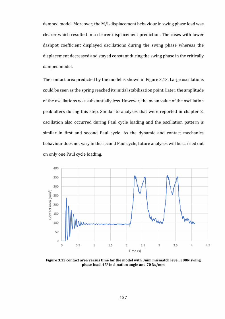
127

damped model. Moreover, the M/L displacement behaviour in swing phase load was

clearer which resulted in a clearer displacement prediction. The cases with lower

dashpot coefficient displayed oscillations during the swing phase whereas the

displacement decreased and stayed constant during the swing phase in the critically

damped model.

The contact area predicted by the model is shown in Figure 3.13. Large oscillations

could be seen as the spring reached its initial stabilisation point. Later, the amplitude

of the oscillations was substantially less. However, the mean value of the oscillation

peak alters during this step. Similar to analyses that were reported in chapter 2,

oscillation also occurred during Paul cycle loading and the oscillation pattern is

similar in first and second Paul cycle. As the dynamic and contact mechanics

behaviour does not vary in the second Paul cycle, future analyses will be carried out

on only one Paul cycle loading.

Figure 3.13 contact area versus time for the model with 3mm mismatch level, 300N swing

phase load, 45° inclination angle and 70 Ns/mm

0

50

100

150

200

250

300

350

400

0 0.5 1 1.5 2 2.5 3 3.5 4 4.5

Co

nta

ct a

rea

(mm

2 )

Time (s)

128

3.4.3 Mass effect

Figure 3.14 represents the M/L displacement of the model with true mass values for

the 3mm mismatch case. Zero displacement in the pre-contact and spring

compression steps is expected as no horizontal movement resulted from these

steps. Dashpot coefficients varying between 1 Ns/mm and 4 Ns/mm were tested on

this model. The minimum dashpot coefficient that resulted in no oscillation was 3

Ns/mm. Although the critical value of the dashpot coefficient differed between the

true and artificial mass models, the same damping behaviour is observed for both

mass conditions. The spring seems to become stable in a significantly shorter time

than for the artificial mass values with a minimum level of oscillation. In gait cycle

loading, the M/L displacement with true mass values, as for the artificial mass

values, followed the axial loading changes. The displacement at the peak loads are

the same and no overshooting of the displacement was observed.

Figure 3.14 M/L displacement behaviour for various dashpot coefficient with true mass values, 3mm translational mismatch level and 300N swing phase load

Figure 3.15 indicates the difference in M/L displacement under cyclic load when

artificial and true mass values are applied. Although the overall M/L displacement

-0.7

-0.6

-0.5

-0.4

-0.3

-0.2

-0.1

0

0 0.2 0.4 0.6 0.8 1 1.2 1.4

M/L

dis

pla

cem

ent

(mm

)

Time (s)Dashpot coefficient of 1 dashpot coefficient of 3 Dashpot coefficient of 4

129

pattern is similar in both cases, the following differences between the true and

artificial mass model with respect to the M/L displacement were observed:

Time delay in M/L displacement response only in model with artificial mass

value.

Different M/L displacement value for two peaks in the model with artificial mass

value whereas true mass values resulted in the same M/L displacement for both

peaks.

During the swing phase, the analysis carried out on the model with true mass

values resulted in constant M/L displacement. However, the artificial mass value

resulted in gradual decrease in M/L displacement throughout the whole swing

phase.

Figure 3.15 Critically damped model of artificial and true mass on M/L displacement behaviour with sampling frequency of 20 with 300N swing phase load and 3mm

translational mismatch level

The contact area predicted by both models (Figure 3.16) showed the same

numerical noise. However, the amplitude of the noise is very small and the general

trend of contact area is obvious. The major differences in contact area between the

cases occurred at the beginning of the stance phase and during the swing phase. The

0

500

1000

1500

2000

2500

3000

3500

-0.6

-0.5

-0.4

-0.3

-0.2

-0.1

0

0 0.2 0.4 0.6 0.8 1 1.2

Load

(N

)

M/L

dis

pla

cem

ent(

mm

)

Time (s)

True mass values Artificial mass value Paul cycle loading

130

analysis with true mass values resulted in a slightly higher contact area as the load

reached its first peak. Moreover, contact area changes during the swing phase in the

artificial mass model gradually decreased whereas the contact area in the true mass

model is constant throughout the swing phase.

Figure 3.16 Contact area comparison using true and artificial mass values for the analyses

with 3mm translational mismatch level and 300N swing phase load

3.4.4 Model input sensitivity

The two cases that could represent the best and the most crucial output conditions

(1mm and 4mm mismatch) were analysed and the M/L displacement time history

for each is presented in Figure 3.17. Once more, the expected behaviour was seen

for each of the pre-contact, spring compression and stabilisation steps and the

analyses were critically damped so no oscillation or long term gradual stabilisation

was observed. The general trend of the M/L displacement in all the cases followed

the axial loading changes and the M/L displacement behaviour seemed to be similar

to the previous analysis with 3mm mismatch level and critically damped system.

0

50

100

150

200

250

300

350

400

0 0.1 0.2 0.3 0.4 0.5 0.6 0.7 0.8 0.9 1

Co

nta

ct a

rea

(mm

2 )

Time (s)

Artificial mass value True mass value

131

Figure 3.17 The M/L displacement of the cases that represent the analyses with 1mm and

4mm translational mismatch level, 45° inclination angle and 300N swing phase load

The contact area changes during Paul cycle loading for the 1mm and 4mm mismatch

level is presented in Figure 3.18. Both analyses resulted in virtually the same

maximum contact area at the peak loads. However, the contact area derived during

the swing phase was less for the 4mm mismatch than for the 1mm mismatch. The

difference in contact area value during the swing phase agreed with the changes in

M/L displacement. The difference in contact area occurred due to the higher lateral

separation in 4mm mismatch case resulting in a smaller contact area close to the

lateral edge of the cup.

Figure 3.18 Contact area derived from analyses versus time with 300N swing phase load, 45o

inclination angle and translational mismatch variation of 1mm and 4mm

-3

-2.5

-2

-1.5

-1

-0.5

0

0 0.2 0.4 0.6 0.8 1 1.2 1.4

M/L

dis

lpla

cem

ent

(mm

)

Time (s)

1mm mismatch 4mm mismatch

0

50

100

150

200

250

300

350

400

0 0.2 0.4 0.6 0.8 1 1.2

Co

nta

ct a

rea

(mm

2 )

Time (s)1mm mismatch 4mm mismatch level

132

3.5 Discussion

The analyses reported in this chapter focused on the reliability of the chosen

methods based on the applications. The model is required to predict the level of M/L

displacement for validation proposes against in vitro testing as described in the next

chapter. Once the model is validated against in vitro studies, the reliability of the

model can be assured in order to predict the effect of a wide range of parameters on

the dynamic and contact mechanics of the THRs. As dynamic separation and edge

loading are multifactorial scenarios (Fisher, 2011), in vitro studies are expensive

and it is time consuming to test all the potential factors or combination of the factors

on THR behaviour due to simulator preparation time, long duration of simulator

testing, maintenance of the simulators and number of tests required. However, a

validated computational model can provide a useful insight to the THR performance

during an activity. A wide range of parametric testing can also be carried out on the

computational models to estimate which parameters can potentially have the most

effect on the THR performance under adverse conditions. Furthermore, those

parameters can be taken forward in experimental studies.

The computational model also needs to estimate reliable contact mechanics

information. The contact mechanics output provides information about which area

of the bearing undergoes the most severe contact behaviour that could lead to

permanent damage and potentially failure of the device. The model can be used to

determine at which stage of the gait cycle the bearing is potentially at the most risk

of damage. The insight from the contact mechanics information about the bearing

behaviour during an activity helps to navigate and focus on the damaged zone for

improvement of future joint designs.

133

In vitro studies cannot provide contact mechanics information for the bearing

during a gait cycle. The dynamic parameter that is measured in these simulator

studies is the dynamic separation within the cycle. Therefore, the dynamic

separation is the only factor that can be readily compared between the in vitro and

computational studies. In this chapter, the computational model is developed to

simulate the experimental configuration simply by considering the efficiency of the

computational method.

There is an element of damping (energy loss) due to mechanical friction or other

tribological effects in all real systems. In the simulators, no additional damping is

attached to the spring and the damping in the experimental studies is provided by

friction and other aspects of the total components behaviour such as mass.

Therefore, there is no direct measurement of the damping in the experimental set

up and it is a very challenging task to quantify the in vitro damping. In computational

studies, damping is modelled mathematically to align the model more closely to the

real-world scenario and to reduce the system noise. In this application, as the spring

is the primary cause of the oscillation in the M/L displacement, the damping is

directly applied by adding a damper parallel with the spring.

There are different numerical damping methods that were discussed in the technical

background section of this chapter. Bulk viscosity applies the damping to the whole

system regardless of the individual components. ABAQUS applies a small level of

bulk viscosity by default to decrease the numerical noise of the system. Material

damping can be applied only when using a truss element as the spring. However, the

prediction of mass and stiffness proportional Rayleigh damping is very challenging

for a system with many degrees of freedom. The most ideal option is to add the

134

discrete dashpot to be used in parallel with spring element to add damping in

addition to the default bulk viscosity damping.

The spring/dashpot system is the simplest method to implement the experimental

spring behaviour as it only requires a simple calculation prior to analysis whereas

the material damping/truss element system requires a complex initial calculation to

find the Rayleigh damping factors. On the other hand, the spring element is not

considered in the ABAQUS stability time step calculation due to the lack of spring

element mass. This could cause a level of instability in the whole system. This effect

is substantial when considering a damper/spring system because of continuous

spring movement. However, the spring/dashpot system does not appear to

experience any dynamic instability throughout the analysis although numerical

oscillation still occurs for low values of dashpot coefficients

The damping conditions have a great effect on the M/L displacement of the model.

Maximum M/L displacement (during the swing phase) varies based on the damping

factor. The critically damped model predicts the maximum M/L displacement with

no oscillations present. The results from an over/under damped system are not as

reliable as from the critically damped model as the dynamic effects could potentially

be underestimated in the over damped system and overestimated in the

underdamped system. There is not a specified level of damping that can be extracted

from the experimental set up. If a fixed dashpot coefficient is assigned for all the

cases, it could either be an estimation or predicted from the certain conditions based

on the experimental behaviour. However, this approach is challenging as it

would involve a whole series of analyses to be carried out at much longer

computational time and cost.

135

As increased mass has the inverse effect on the time increments for stability, the

effect of mass scaling was examined to shorten the running time of the analysis. The

main effect of mass on the dynamics of the model is during the swing phase. The

M/L displacement during the swing phase seems to be constant in the analysis with

true mass values as the swing phase load is constant. However, artificial mass values

resulted in continuous increase in M/L displacement during the swing phase. Higher

mass values results in longer time to stabilise the output than true mass values. The

asymptotic behaviour of M/L displacement during the swing phase for the artificial

mass model could be explained by the lack of sufficient time during the swing phase

to reach a stable value.

Artificial mass values also result in substantial changes in the M/L displacement

between the two peak loads during the stance phase whereas true mass values cause

only a slight change during that time. This difference in dynamic behaviour is due to

the inertia in two systems. True mass values results in lower inertia and therefore,

takes less time to settle to a stable position than higher inertia for the artificial mass

model. For future analyses, true mass values for all the components are specified as

the differences between the M/L displacement in the true and artificial mass

analyses are substantial even though the run time of the true mass analyses are

much higher.

In the model input sensitivity study, the analyses positively reacted to the changes

in the cases. There was a definite differentiation between the attempted cases. As

expected, the maximum M/L displacement increased as the translational mismatch

level increased. Moreover, no oscillations or instability of the dynamic and contact

mechanics data were observed throughout the analyses when critical damping was

applied. Although no noise in the analysis simplified the output reading, pre-

136

damping analysis is required for each case to predict the dashpot coefficient level

that produce a critically damped system. The output observation indicated an

acceptable overall dynamic and contact mechanics behaviour. Therefore, the next

step would be validating the output by comparison with in vitro data followed by

parametric testing.

3.6 Key findings

ABAQUS built in spring element with dashpot in parallel was found to be the best

method to represent the in vitro spring.

The dynamic and contact mechanic are directly affected by the mass of the

system. Therefore, true mass values will be applied to the model for all future

analyses even though the run time was over 20 hours for the analyses with true

mass values.

As determined, the true damping ratio of the simulator is a challenging task,

critically damping was assigned to the spring to minimise oscillation of the M/L

displacement. However, damping calibration is required for each individual

cases to reach critically damped model.

The M/L displacement of the model behaved expectedly. Therefore, the next step

is to perform model validation and parametric testing.

137

Chapter 4 Parametric sweep, validation and sensitivity

testing

4.1 Introduction

In line with the conclusion of Chapter 3, the method of the explicit finite element

model of THR under adverse condition is mainly developed and finalised. The

agreed method consisted of a spring element that initially is compressed for the

desired translational mismatch level and then is released to maintain the stability.

After the stabilisation of the spring, the model is loaded with the gait cycle axially.

Implying the dashpot coefficient assisted the model to eliminate the effect of noise

on the results. The recorded separation had an inverse relationship with the loading

during the gait cycle which resulted in the highest separation during swing phase

and consequently, the lowest contact area in the cycle.

The results that were exported from the chosen method followed the sensible trends

as the experimental methodologies, and so enabled the next step of the development

which was applying the parametric sweep of testing and validate the outcome

against in vitro studies. The aim of testing parametric sweep and validation was to

test the reliability of the method that leads to confidence in the conclusion resulted

from the model output.

The parametric sweep focussed on the following key areas:

1 Translational mismatch level: A level of mismatch between the centre of the

head and the cup

2 Rotational variation: variation in cup inclination angle

3 Tissue laxity: by varying swing phase load

138

In this chapter, the dynamic effect of the parameters such as dynamic separation

predicted by the finite element model is compared to separation values measured

in independent in vitro tests undertaken by another researcher (Ali et al, 2016;

Appendix). The results from thirty two independent conditions data points were

compared to the experimental results for the same set of conditions as part of the

validation process.

The validation of the model is discussed based on the in vitro testing carried out on

an iMBE electromechanical hip simulator (Prosim EM13 hip simulator) which has

previously been used to test metal on polyethylene hips under standard conditions.

For the purposes of the validation of this computational model of edge loading, the

test conditions and study reported in the Appendix was used, As the model is set to

replicate a physical hip simulator, the overall assembly of the experimental set up

was replicated in the computational model to simplify the validation process.

Furthermore, as friction occurs in the bearing in the experimental simulator and the

precise value is not known, the model was tested for sensitivity to variation in the

coefficient of friction on the contact surfaces was carried out on the model to

understand the effect of friction on the extreme cases in the input parameters.

Friction and lubrication of the bearing materials have an effect on the contact

mechanics and wear of the material bearings in vitro studies (Brocket et al, 2007).

The aim of the sensitivity test is to examine if friction at the bearing surfaces plays

an important role in this application.

The layout of this chapter also, consists of the description of the methodology

(section 4.2), the computational and experimental result presentation (section 4.3),

discussion of the results (section 4.4) and the key finding of the studies (4.5),

respectively.

139

4.2 Methodology

The model specification used in these analyses is fully described in previous

chapters. The geometry, material properties, assembly, contact conditions,

boundary conditions and element size are described in Chapter 3 methodology. To

summarize the model development, Figure 4.1 represents the assembly of the

components in the model.

Figure 4.1 The assembly of the components in the computational model for the parametric testing purposes

Furthermore, the material properties of the components and meshing

configurations are available in Table 4.1 and Table 4.2, respectively.

Table 4.1 Material properties of the components the computational analyses in the parametric sweep of chapter 4

Components Material Young’s modulus

(MPa)

Poisson’s ratio

Density (kg/mm3)

Outer radius (mm)

Inner radius (mm)

Head Rigid - - 4.37x10-9 18 -

Cup Polyethylene 670

(Elasticity) 0.46 9.23x10-10 - 18.524

Shell Titanium 114,500 0.34 4.43x10-9 56 -

Cup holder Rigid - - 8.5x10-10 27.25 24.25

140

Table 4.2 The meshing configurations and the element size of the components in the computational analyses in the parametric sweep of chapter 4

Component Global size (mm) Element shape Code Number of

elements

Head 1.5 Hexahedral R3D4 2,228

Cup 1.5 Hexahedral C3D8R 8,960

Cup holder 3 Hexahedral and

tetrahedral

R3D4 and

R3D3 2,211

Shell 2 Hexahedral C3D8R 2,820

Moreover, the same set of progressive dynamic steps and boundary conditions

which are presented in chapter 3 is used and presented in Table 4.3.

Table 4.3 The boundary and loading conditions on each step of the computational analyses in the parametric sweep of chapter 4

Steps Duration Axial load

Boundary conditions

Head movement

Cup movement

Spring movement

Lateral end Medial end

Pre-contact 0.05 - 0.542mm

upward Fixed Fixed Fixed

Spring compression

0.05 - Fixed Fixed Fixed Spring

compression

Spring stabilisation

Alters Constant

300N Fixed

Horizontal and vertical translation


Fixed

Loading 2 2 Paul cycle

Fixed Horizontal

and vertical translation


Fixed

141

4.2.1 Input parameters

For validation purposes, the same input parameters that were tested

experimentally, surgical translational mismatch, rotational variation and tissue

laxity, were adjusted to the models as an input (Appendix).

Table 4.4 is the matrix describing the full set of test cases that were carried out in

this chapter. For the parameter sweep study, total of 32 cases with variety in

translational, rotational variation and swing phase were carried out. Moreover, the

cases which friction studies were tested on are also shown. The running time taken

to carry out each of the analysis was approximately 21 hours.

Table 4.4 The full set of test cases in the parameter sweep based on various translational mismatch level, swing phase load and cup inclination angle

The implementations of input parameters that are mentioned in Table 4.4 are

explained as follows:

Surgical translational mismatch: The translational mismatch level is presented in

the model by setting a mismatch between the centre of the head and cup which

causes the spring to compress. The same translational mismatch level of 1mm, 2mm,

3mm and 4mm, that were used experimentally, were applied. Surgical translational

142

mismatch represents a level of mismatch between the cup and the head centre.

Figure 4.2 represents the schematic of translational mismatch level in the

computational model

Figure 4.2 The difference in assembly of fully concentric (A) where the head and the cup

have the same centre and THR bearing with translational mismatch level (B) where there is a translational distance between the bearing centres

Surgical rotational variation: Surgical rotational variation effect has been studied

in vitro by varying the cup inclination angle. Two different cup inclination angles are

tested in vitro: 1) 45° inclination angle that is assumed to be in the safe zone and 2)

65° inclination angle which is defined as a steep inclination angle. To apply surgical

rotational variation, the polyethylene cup, metal shell and the cup holder are

assembled to have 35° angle with respect to horizontal axis to represent 45° clinical

inclination angle. To implement a surgical rotational mismatch of 65°, the inclination

angle of 55° is applied (Figure 4.3). The 10° difference between the cup inclination

angles clinically and experimentally is due to the difference in loading angle in vitro

and in vivo (explained in chapter 2). The cup inclination angle reported throughout

this chapter is referenced to the clinical cup inclination angle.

143

Figure 4.3 Rotational mismatch configuration. A) 45° inclination angle clinically B) 65°

inclination angle clinically

Tissue laxity: Tissue and muscle laxity seen in vivo, is represented in vitro and in

silico by varying the swing phase load of the gait cycle. The swing phase loads of 70N,

100N, 200N and 300N are tested in vitro which is within the range of patient’s swing

phase load range in the Bergsmann study (Bergmann et al., 2001). The same

experimental variation of swing phase loads are applied to the model. The gait cycle

loading of each case which is extracted from experimental testing is presented in

Figure 4.4.

Figure 4.4 The input gait cycle loading versus time for each swing phase load of 70N, 100N,

200N and 300N

0

500

1000

1500

2000

2500

3000

3500

0.000 0.200 0.400 0.600 0.800 1.000 1.200

Load

(N

)

Time (s)

70N swing phase load 100N swing phase load

200N swing phase load 300N swing phase load

144

Case-specific model specifications: The constant force that was applied during

stabilisation time (to fasten the stabilisation) differs from each condition to match

the swing phase loads applied throughout the gait cycle of the specific analysis.

In line with the conclusion of Chapter 3, the choice of dashpot coefficient for critical

damping of the spring was affected by the mass of the system the translational

mismatch level (due to the variation in the resultant force and the cup position in

relation to the head). In these analyses, although the mass of the system was

constant, the translational mismatch was varied. It is expected that this will result

in variation of the coefficient of damping between cases, so an initial dashpot

coefficient analysis was carried out to achieve critically damped spring in each case.

The table of dashpot coefficient for analysis carried out with 45° inclination angle is

presented in Table 4.5 and 65° inclination angle is represented in Table 4.6. Before

gait cycle loading, a series of analyses were carried out on each condition to achieve

a critically damped system.

Table 4.5 Dashpot coefficient of analysis with 45° inclination angle, translational mismatch level of 1mm to 4mm and swing phase load of 70N to 300N

Mismatch (mm) 70N 100N 200N 300N

1 1.85 1.8 2.1 2.5

2 1.5 1.8 1.4 2.35

3 1.2 1.1 2.25 3.1

4 1.1 1.2 1.2 1.3

Table 4.6 Dashpot coefficient of analysis with 65° inclination angle, translational mismatch level of 1mm to 4mm and swing phase load of 70N to 300N

Mismatch (mm) 70N 100N 200N 300N

1 1.25 1.4 1.35 2.5

2 1.5 1.1 1.4 2.1

3 1.2 1.2 1.1 1

4 1 1.1 1 0.8

145

4.2.2 Outputs and experimental comparison

4.2.2.1 Maximum dynamic separation

The highest dynamic separation value throughout the gait cycle which occurs during

the swing phase load was recorded for validation purposes.

Edge loading definition: If the maximum dynamic separation was greater than the

radial clearance (0.5mm), the separation is defined to cause head contact with the

rim of the cup and a level of edge loading.

Experimental measurement: The in vitro dynamic separation was recorded from

the biomechanical testing on Pinnacle metal-on-polyethylene THRs on the

electromechanical hip simulator (EM13). The experimental maximum separation

was taken as the mean value of the separation recorded from three samples. For the

validation and comparison purposes, the maximum dynamic separation was

exported from the explicit finite element model. The dynamic separation in vitro was

measured from the point where the cup and the head were in contact with no spring

compression (Figure 4.5).

Figure 4.5 The schematic of dynamic separation measurement in vitro. A) The point where the separation is measured from (concentric cup and head and no spring compression), B)

Minimum dynamic separation and C) Maximum dynamic separation (edge loading)

4.2.2.2 Maximum load at the rim

In the conditions that edge loading occurs, the maximum load that the rim of the cup

undergoes, is recorded in two different time points:

146

1. When the input load is increasing to the first peak and the head is relocating to

the concentric condition.

2. When the input load is decreasing from the second peak to the swing phase load

and the head is separating from the concentric condition.

Computational measurement: to calculate the load at the rim, firstly, the point at

which the separation is at the minimum level (including 0.5mm) is recorded.

Secondly, the corresponding time point in which the separation would be 0.5mm is

calculated by using linear interpolation. Finally, the input load at the time in which

the recorded separation level occurred is measured. Figure 4.6 illustrates the time

point at which the separation and the load are measured.

Figure 4.6 The intersection of the load and the separation for maximum load at the rim calculations. The corresponding load to the dynamic separation of 0.5mm is recorded as the maximum load at the rim

Experimental measurement: The experimental measurement method used to

determine maximum load at the rim was similar to the computational measurement.

The load at the rim was determined as the axial force measured from the load cell at

147

a specified dynamic separation (Appendix). However, the maximum load at the rim

is only taken when the head is relocating to the concentric condition.

4.2.3 Friction sensitivity test

Four cases were selected for a friction sensitivity test, where a friction coefficient of

0.1 was applied to the contact between the bearings surfaces based on the range of

friction coefficient of the bearing presented in the study by Jin et al (2006). The

selected cases are marked in Table 4.4. The difference in the separation data output

between the computational and experimental results for these cases was the

highest. Friction testing was carried out specifically on these cases to see if the

difference between the results could be explained by friction. Based on the dynamic

separation of the all conditions, the friction analyses were carried out on the chosen

one due to their dynamic behaviours. The friction testing was carried out on the four

conditions with:

4mm translational mismatch

70N and 300N swing phase load

45° and 65° cup inclination angles

148

4.3 Results

This section of chapter is divided into three sections that firstly focus on the dynamic

results of the computational model. Secondly, the comparison and validation of the

computational results against the experimental testing is carried out. Finally, the

effect of friction in the bearing on the selected conditions are described.

4.3.1 In silico parameter sweep

The in silico maximum dynamic separation caused by surgical translational

mismatch level, rotational variation and swing phase load of the THR are all plotted

and compared. Figure 4.7 represents the maximum dynamic separation resulted

from various translational mismatch and swing phase loads in 45 cup inclination

angle. For this cup inclination angle, the combination of 1mm translational

mismatch level and 300N swing phase load results in a best separation case

(0.1mm). Moreover, the worst separation case (3.1mm) occurred with the

combination conditions of 4mm mismatch level and 70N swing phase load. The

separation increased as the translational mismatch increased for a fixed swing

phase load. Also, increase in swing phase load for a specific translational mismatch

decreased the separation level. Based on the definition of the edge loading that was

defined in methodology (section 4.2), 7 out of 16 conditions underwent a separation

of greater than 0.5mm and some degree of edge loading with 45 inclination angle.

149

Figure 4.7 Maximum dynamic separation versus the variation of translational mismatch levels (1mm to 4mm) and swing phase loads (70N to 300N) and 45 inclination angle

Figure 4.8 illustrates the maximum dynamic separation of various translational and

swing phase loads in 65 cup inclination angle. The same trend of the lowest and

highest separation levels were observed in the similar cases as 45 inclination angle.

However, the range of separation level varies from 0.1mm to 3.5mm. Moreover,

lower swing phase load and higher translational mismatch level resulted in higher

separation levels. In 65 inclination angle conditions, a separation of greater than

0.5mm and some degree of edge loading occurred in 11 out of 16 conditions.

1mm

2mm

3mm

4mm

0

0.5

1

1.5

2

2.5

3

3.5

70 100 200 300

Tran

slat

ion

al m

ism

atch

leve

l

Max

imu

m d

ynam

ic s

epar

atio

n (

mm

)

Swing phase load (N)

150

Figure 4.8 Maximum dynamic separation versus the variation of translational mismatch levels (1mm to 4mm) and swing phase loads (70N to 300N) and 65 inclination angle

Furthermore, the effect of cup inclination angle on maximum dynamic separation

was considered. As Figure 4.9 shows, a 70N swing phase load produced dynamic

separation of 0.4mm to 3.1mm under standard cup inclination angle (45°) and

0.5mm to 3.6mm for steep inclination angle (65°). The dynamic separation level

increased as the translational mismatch level increased in both cup inclination

configurations. Steeper cup inclination angle results in a higher dynamic separation

than standard cup inclination angle for different translational mismatch level.

1mm

2mm

3mm

4mm

0

0.5

1

1.5

2

2.5

3

3.5

4

70 100 200 300

Tran

slat

ion

al m

ism

atch

leve

l

Max

imu

m d

ynam

ic s

epar

atio

n (

mm

)


151

Figure 4.9 The effect of standard and steep cup inclination and translational mismatch of 1mm to 4mm on the maximum computational dynamic separation with 70N swing phase

load

Figure 4.10 illustrates that the same trend of maximum dynamic separation changes

occurred for different cup inclination angles when 300N swing phase load was

applied. Although the dynamic separation increased as the translational mismatch

level increased for both cup inclination angle, the maximum dynamic separation for

all translational mismatch level for 45° inclination angle is less than 0.5mm (radial

clearance). The maximum dynamic separation with 65° inclination angle increased

substantially as the dynamic separation became greater than radial clearance (up to

2.45mm separation). Additionally separation of greater than 0.5mm and edge

loading occurred more frequently with the 65 degree inclination angle.

0

0.5

1

1.5

2

2.5

3

3.5

4

1 2 3 4

Max

imu

m d

ynam

ic s

epar

atio

n (

mm

)

Mismatch level (mm)

45 dgree inclination angle 65 degree inclination angle

152

Figure 4.10 The effect of cup inclination and translational mismatch on the maximum

computational dynamic separation with 300N swing phase load

4.3.2 Comparison of in vitro and in silico

Figure 4.11 illustrates the overall comparison of computational and experimental

maximum dynamic separation value for all the frictionless cases tested. As

Figure 4.11 demonstrates, mostly, the model overestimated the separation level

compared to the experimental values. The results indicated that there is an

overestimation of the separation by the computational model for high separation

levels and slight underestimation of the separation by the computational model for

lower separation level.

This graph doesn’t present the specific separation level under different translational

mismatch level which indicates that the overestimation of the separation doesn’t

seem to be only dependant on the cup inclination angle or swing phase load.

Figure 4.11 does not represent the variation of the separation level in experimental

testing and the variation will be demonstrated later in this chapter.

0

0.5

1

1.5

2

2.5

3

1 2 3 4

Max

imu

m d

ynam

ic s

epar

atio

n (

mm

)

Mismatch level (mm)

45 degree up inclination angle 65 degree cup inclination angle

153

Figure 4.11 Comparison of computational dynamic separation and experimental dynamic separation. The legend represents the swing phase load

and the cup inclination angle. Standard is referred to 45o inclination angle and steep is referred to 65o inclination angle

0

0.5

1

1.5

2

2.5

3

3.5

4

0 0.5 1 1.5 2 2.5 3 3.5 4

Exp

erim

enta

l sep

erat

ion

(m

m)

Computational separation (mm)

70N, standard

100N, standard

200N, standard

300N, standard

70N, steep

100N, steep

200N, steep

300N, steep

154

Figure 4.12 and Figure 4.13 illustrate the maximum dynamic separation versus the

surgical translational mismatch for different swing phase loads under standard cup

inclination angle and steep inclination angle, respectively. The bars on the

experimental data represents the variation of maximum separation in in vitro

testing.

The comparison of computational and experimental separation for standard cup

inclination angle indicates that the separation predictions are in a good agreement

for all the translational mismatch levels in a higher swing phase loads than lower

swing phase loads. The most overestimation occurs for the cases with low swing

phase loads especially high translational mismatch levels (70N and 100N).

In standard cup inclination angle condition, it is difficult to compare the separation

values under 1mm translational mismatch level because the experimental result

does not vary considerably due to a low separation level. There is a good agreement

for all swing phase loads when 2mm translational mismatch was applied except 70N

swing phase load. The experimental value does not follow the actual theoretical

trend in this specific case (the experimental separation does not increase as the

swing phase decreases). In the cases with 3mm and 4mm translational mismatch

level, good agreement was seen under high swing phase loads (200N and 300N).

However, the most overestimation was observed under low swing phase loads.

155

Figure 4.12 The effect of translational mismatch and swing phase load on the maximum

dynamic separation of the THR in vitro and in silica under 45° inclination angle. The letters E and C in the legend section represents experimental and computational data, respectively

(in vitro testing was carried out by Murat Ali, Appendix)

Figure 4.13 indicates the computational maximum dynamic separation of up to

0.5mm for 1mm mismatch level, 1.55mm for 2mm, 2.55mm for 3mm and 3.55mm

for 4mm translational mismatch level in steep cup inclination angle. The inverse

relationship between swing phase load and maximum dynamic separation is also

observed for a fixed translational mismatch level. In contrast to standard cup

inclination angle, there is a great agreement between the experimental and

computational separation when lower swing phase loads were applied (70N and

100N). Furthermore, higher swing phase loads (200N and 300N) resulted in the

overestimation of the computational separation. Although, there an overestimation

of the output, the experimental and computational separation follow a similar trend

between the different conditions. The potential reasons for the differences between

the computational model and the experimental results are described in the

discussion

0

0.5

1

1.5

2

2.5

3

3.5

1 2 3 4

Max

imu

m s

epar

atio

n (

mm

)

Translational mismatch (mm)

C 70N E 70N C 100N E 100N C 200N E 200N C 300N E 300N

156

Figure 4.13 The effect of translational mismatch and swing phase load on the maximum dynamic separation of the THR in vitro and in silica under 65° inclination angle. The letters E

and C in the legend section represents experimental and computational data, respectively (in vitro testing was carried out by Murat Ali, Appendix)

4.3.3 Friction sensitivity test

The effect of friction on the maximum dynamic separation is also studied. The

maximum separation generated by using friction coefficient of 0.1 under the

specified conditions are presented in Figure 4.14. As the dynamic separation of the

chosen conditions show, the maximum overestimation of the separation occurred

under standard cup inclination angle, 4mm translational mismatch level and 70N

swing phase load. And also under steep cup inclination angle, 4mm translational

mismatch level and 300N swing phase load. Therefore, primarily these conditions

were chosen for friction analysis. Moreover, friction analyses were carried out on

two other conditions (same translational mismatch level with 70N and 300N swing

phase load under steep and standard cup inclination angle, respectively) to

understand if friction could affect the level of validation agreement for these cases.

0

0.5

1

1.5

2

2.5

3

3.5

4

4.5

1 2 3 4

Max

M/L

dis

pla

cem

ent

(mm

)

Mismatch (mm)

C 70N E 70N C 100N E 100N C 200N E 200N C 300N E 300N

157

Figure 4.14 Comparison of computational and experimental maximum dynamic separation under steep inclination angle (friction coefficient of 0.1). Experimental bars represents the

dynamic separation in vitro, Computational bars represent the maximm dynamic separation with friction coefficient of 0.1 between the contact surfaces and computational frictionless

bars represents the maximum dynamic separation with no friction between the contact surfaces

Slightly reduced maximum dynamic separation was obtained in the both standard

cup inclination conditions and 70N swing phase load under steep cup inclination

angle. However, the bearing friction in the model had a great effect on the level of

dynamic separation for the higher swing phase load under steep cup inclination

angle (0.8mm reduction).

As Figure 4.14 demonstrates, although friction coefficient decreased the maximum

dynamic separation in comparison with frictionless analyses, the underestimation

of the computational dynamic separation in comparison with experimental results

is still observed on the same cases as frictionless analyses.

4.3.4 Maximum load at the rim

In this section, the comparison of the maximum force on the rim of computational

and experimental data is shown. Firstly, the computational maximum force on rim

for 45 and 65 inclination angles are presented in Figure 4.15 and Figure 4.16,

respectively. As Figure 4.15 illustrates, the maximum force on the rim under

0

0.5

1

1.5

2

2.5

3

3.5

4

4.5

standard cup inclination,300N

standard cup inclination,70N

Steep cup inclination,300N

Steep cup inclination,70N

Max

imu

m m

edia

l/la

tera

l dis

pla

cem

ent

(mm

)

Experimental Computational Computational frictionless

158

standard cup inclination varies between zero to 1980N. As it was described in

methodology, no edge loading was assumed for the conditions which had separation

level of less than 0.5mm. Therefore, the maximum force on the rim for these

conditions are shown in graph with no load at the rim. However, the maximum force

on the rim increased by increasing the swing phase load and increasing the

translational mismatch level.

Figure 4.15 Computational maximum force on the rim with different translational mismatch

level and swing phase loads under 45 inclination angle

The range of maximum force on the rim for all the conditions under steep cup

inclination angle (Figure 4.16) is demonstrated to be between zero to 2020N. The

similar trend that was found with standard cup inclination angle was also found

with steep cup inclination angle. Therefore, higher swing phase load and higher

translational mismatch level increased the value of maximum load at the rim.

However, the swing phase load did not have a substantial effect when 4mm

translational mismatch was applied.

1

2

3

4

0

200

400

600

800

1000

1200

1400

1600

1800

2000

70N 100N 200N 300N

Tran

slat

ion

al m

ism

atch

leve

l (m

m)

Load

(N

)


159

Figure 4.16 Computational maximum force on the rim versus translational mismatch level

of 1mm to 4mm and swing phase loads under 65 inclination angle

In the next step, the maximum load at the rim at the relocation to concentric point

from the edge and the separation from the concentric point to the edge were

compared. As Figure 4.17 represents, under standard cup inclination angle, the

maximum load at the rim at the relocation time is substantially higher than the

separation time. When the head is relocating into the concentric condition, the

maximum load at the rim could be five times higher than the load at the rim when

the head is separating from the cup. The conditions that have the similar relocation

and separation maximum load at the rim contain high swing phase load (200N with

3mm mismatch and 300N).

1

2

3

4

0

500

1000

1500

2000

2500

70N 100N 200N 300N

Tran

slat

ion

al m

ism

atch

leve

l (m

m)

Load

(N

)


160

Figure 4.17 Comparison of the load the rim when the head is moving to concentric condition and when the head is moving to the edge under standard cup inclination angle. At the legend

of this graph, the word ‘in’ represents the maximum load at the rim when the head was relocating into the cup and the word ‘out’ represents the maximum load at the rim when the

head was separating out of the concentric point

Similar observation could be seen from the maximum load at the rim comparison

under steep cup inclination angle. However, all the conditions resulted in a

substantially higher maximum load at the rim at the relocation point than the

separation point. The range of maximum load at the rim at the relocation point is

between zero to 2020 whereas the maximum load at the rim at the separation point

is between zero to 800N.

0

500

1000

1500

2000

2500

1 2 3 4

Load

(N

)

Translational mismatch level (mm)

Out 300N In 300N Out 200N In 200N Out 100N In 100N Out 70N In 70N

161

Figure 4.18 Comparison of the load the rim when the head is moving to concentric condition and when the head is moving to the edge under steep cup inclination angle. At the legend of

this graph, the word ‘in’ represents the maximum load at the rim when the head was relocating into the cup and the word ‘out’ represents the maximum load at the rim when the

head was separating out of the concentric point

The difference between the computational and experimental maximum load at the

rim was also studied. The maximum force on the rim is dependent on the occurrence

of edge loading. If the separation is less than 0.5mm, the maximum force on the rim

is not calculated in vitro as there is no contact of the head with rim surface.

Therefore, the computational maximum load at the rim that are presented in the

following figures are for the available experimental maximum load at the rim

conditions. No maximum load at the rim was found in in vitro studies for 1mm and

2mm translational mismatch level. Then, the comparison graphs only illustrate the

maximum load at the rim for 3mm and 4mm translational mismatch levels.

Figure 4.19 represents the maximum force on the rim under 70N swing phase load.

The computational method produce substantially higher maximum load at the rim

than the experimental load at the rim. However, lower mismatch level and cup

0

500

1000

1500

2000

2500

1 2 3 4

Load

(N

)


Out 300N In 300N Out 200N In 200N Out 100N In 100N Out 70N In 70N

162

inclination angle decreased the load at the rim in both computational and

experimental methods.

Figure 4.19 Experimental and computational maximum force on the rim under 70N swing phase load, standard (45o) and steep (65o) cup inclination angle, and 3mm and 4mm

translational mismatch level (Appendix)

The same trend of experimental and computational maximum load at the rim for

70N swing phase load (Figure 4.20) was found for 100N swing phase load. The

overestimation of the computational load at the rim occurred. However, both

experimental and computational methods agreed that the load at the rim decreased

as the translational mismatch level and inclination angle decreased.

0

500

1000

1500

2000

2500

3 4

Load

(N

)


Experimental 45 degree inclination angle Computational 45 degree inclination angle

Experimental 65 degree inclination angle Computational 65 inclination angle

163

Figure 4.20 Experimental and computational maximum force on the rim under 100N swing

phase load, standard (45o) and steep (65o) cup inclination angle, and 3mm and 4mm translational mismatch level (Appendix)

The comparison of the maximum load on the head for 200N swing phase load

(Figure 4.21) also indicates the same trend as previous analyses between the

experimental and computational data. However, no load at the rim occurred

experimentally under standard cup inclination angle.

Figure 4.21 Experimental and computational maximum force on the rim under 200N swing

phase load, standard (45o) and steep (65o) cup inclination angle, and 3mm and 4mm translational mismatch level (Appendix)

0

500

1000

1500

2000

2500

3 4

Load

(N

)



Experimental 65 inclination angle Computational 65 degree inclination angle

0

500

1000

1500

2000

2500

3 4

Load

(N

)




164

The rim did not undergo any load under any cup inclination angles when swing

phase load of 300N was applied. Therefore, no experimental and computational

comparison of the maximum load at the rim was carried out with 300N swing phase

load.

165

4.4 Discussion

The dynamic finite element model has been used to predict medial-lateral

separation as it occurred during the gait cycle, including cases where the femoral

head was in contact with the rim of the cup. The development of such a

computational model allows the preclinical testing of THR to examine the factors

that could affect the separation and edge loading the most. Additionally, the validity

of the model has been tested by comparison with an in vitro experimental

simulation. The comparison of experimental and computational results could

indicate if the numerical method is capable of predicting the important dynamics

and contact mechanics data and also giving an overall indication of the model

reliability for future parameters. Therefore, the parameters that have been tested in

vitro experimentally have been applied to the computational model and the effects

of these factors such as surgical translational mismatch, rotational variation and

swing phase load on the dynamic separation are studied.

It has to be recognised both the computational model and the experimental model

are both representations of more complex and variable conditions which occur

clinically, their main value is in predicting the effect of detain biomechanical and

surgical variables on the performance of the hip joint. Direct comparison with the

clinical results can only be made by comparison or wear rates and wear scars and

mechanisms between experimental simulation and retrievals. The development of

the computational model and comparison of the computational and experimental

simulations, will enable wider sets of conditions to be investigated computationally

and more rapidly and most importantly enable the computational models and

predictions to be run in the design phase (including parametric design studies) of

new product development before actual prototypes are manufactured for testing.

166

4.4.1 Computational results

The computational separation results (maximum M/L displacements) indicated the

primary factors that cause more separation level under the same cup inclination

angle are low swing phase load and high translational mismatch. The resultant force

of the medial spring force and the axial force determines the position of the cup with

respect to the head. The combination of low swing phase load (low axial load) and

high medial load causes the edge contact as the cup sits more toward horizontal axis

(Figure 4.22).

Figure 4.22 The cup positioning with respect to the resultant force. A) Resultant force caused

from high swing phase load and low spring force B) Edge contact due to low swing phase load and high spring force

Moreover, the standard cup inclination angle generally causes lower separation

level than steep inclination angle under the similar parameters. In standard cup

inclination angle, the inner curvature of the liner could be acting as a resistance to

the medial movement in comparison with steep cup inclination angle (Figure 4.23).

Additionally, the distance that needs to be travelled by the cup from the concentric

condition to the edge loading condition is longer in standard cup inclination angle

due to the liner edge location with respect to the centre.

167

Figure 4.23 Horizontal travelling distance by the cup with different cup inclination angle. A)

Steep cup inclination angle and B) standard cup inclination angle

It is indicated that the steeper inclination angle and higher spring compression

resulted in increased dynamic separation with the same axial loading (70N swing

phase load). The effect of 20o changes of the inclination angle have the maximum

effect of 0.2mm on the dynamic separation whereas the minimal increase of the

translational mismatch can increase the dynamic separation up to two times. The

same pattern was seen in the previous dynamic computational study that was

carried out on the ceramic-on-ceramic THR (Leng et al., 2017). Therefore, it can be

concluded that translational mismatch has greater effect than rotational variation

on the level of dynamic separation under low swing phase load. However, steep

inclination angle has the greater effect on the dynamic separation if high swing

phase load is applied.

Tissue laxity, which is represented by various swing phase loads, is the other

parameter studied on the computational model. Higher dynamic separation is

achieved by lower swing phase loads for standard cup inclination angle. When

minimum axial load (during swing phase) was applied, the direction of the resultant

force between this force and the medial spring load become closer to the horizontal

axis than vertical axis. Therefore, the resultant force in lower swing phase loads led

168

to greater movement of the cup medial/laterally and higher separation of the cup

with respect to the head.

The maximum load at the rim is affected by the same conditions that affected the

separation. The maximum load at the rim differed for each conditions and higher

translational mismatch level and lower swing phase load increased the maximum

loading at the rim. Also, steeper cup inclination angle affected the load at the rim

negatively. Moreover, it was indicated that there is a substantially higher load at the

rim when the head is relocating to the concentric condition as the load is ramping

up than when the head is separating. Although, the amplitude in load decrease after

the second peak (separating time) is slightly shallower than ramping up

(relocating), the magnitude of the load at the rim should potentially be slightly

affected by it. Such substantially high load at the rim where the contact patch on the

edge is small, could have a more dramatic effect on the contact mechanics of the

bearing such as extreme deformation at the edge contact, wear and material

damage.

4.4.2 Validation

The trend in the dynamic separation changes in the computational model, implies

the overall behaviour of the explicit finite element of THR model under several

parametric testing is plausible. The reliability of the model can be assured by

comparison of in vitro and in silico output. The previous in vitro studies focused on

the wear testing of the THR under only separation (Nevelos et al., 2000, 2001;

Williams et al., 2003; Al-Hajjar et al., 2013). In vitro testing on ceramic-on-ceramic

(O’Dwyer Lancaster-Jones et al., 2017) and metal-on-polyethylene (Appendix) THR

were done in the recent studies to examine the effect of positioning and tissue laxity

on the separation and wear of the bearings. The experimental data in this chapter

169

was extracted from Ali et al studies as the computational analyses were also carried

out on the hard-on-soft bearings. In this comparison, the experimental and

computational dynamic separation follow the same trend of changes with respect to

the tested parameters. However, in some cases there is a disagreement in the

dynamic separation level between the two cases.

The comparison of the experimental and computational dynamic separation and the

load at the rim indicated a level of over/underestimation of the computational

output. However, the difference between the results could be due to various factors.

There is some additional mechanical displacement experimentally and damping in

the loading system, associated with rocking of the cup holders in the mechanical

fixtures and it is not known how this influences the dynamic response in the

experimental system, and this may influence the measurement of the peak load on

the cup, which occurs during a rapidly changing phase of the loading, these three

factors may be expected to realise differences between the experimental and

computational results and be important to explain the differences seen between the

experimental and computational results.

Although the finite element model is designed to replicate the experimental set up,

there are several assumptions that were necessary to make the model viable.

Additionally, hardware tolerances and experimental set up cause variation in the

results produced by practical experimentation. A combination of these factors could

potentially be responsible for the difference in the results.

4.4.2.1 In vitro versus in silico Assumptions

Angular movement: As it was described in chapter 3, there are no angular

movements of the hip applied to the FE model. On the other hand, EM13 simulator

is designed to implement the angular movements on the hip namely

170

flexion/extension, internal/external rotation and abduction/adduction. Because of

spherical geometry of the head, it is assumed that flexion/extension has minimal

effect on the separation. However, the internal/external rotation and

abduction/adduction alter the position of the cup with respect to the head during

the gait cycle. In the testing that were carried out on the EM13 hip simulator

(unpublished data), the dynamic separation varied when 2 axes (flexion/extension

and internal/external rotation) and 3 axes (flexion/extension, internal/external

rotation and abduction/adduction) of rotations were used. Although the degree of

abduction/adduction is lower than the other axes of the rotations (+7/-4) based on

ISO 14242-1:2012 for wear testing on hip simulators, however, the direction of the

movement can possibly give the cup slightly higher contact zone and lower

separation.

Cup translation: the cup can translate in all the directions in the experimental set

up. However, the cup components are computationally constrained to translate in

posterior-anterior and medial-lateral direction. This constraint was stated in

chapter 3. The constraint in transverse plane may slightly affect the edge contact.

Dashpot effect: Before gait cycle implementation, a level of dashpot analysis was

carried out to obtain the coefficient that gave a critically damped system on each of

the conditions. However, the system could yet be slightly

overdamped/underdamped as the dashpot analysis were carried out for certain

amount of times due to long running time of the these analyses. If the system was

not critically damped, the dynamic readings can be slightly affected. However, the

factor should not affect the dynamic results majorly.

Damping of the model: The level of damping in the experimental system should be

the same for all the conditions in experimental testing as the mechanical conditions

171

are the same. However, there is no study so far to understand and predict the level

of damping in vitro or in vivo which makes it extremely challenging to assign a fixed

damping condition for all the computational conditions.

Axial spring: The computational model contains only one spring which is the

medial spring. The experimental EM13 set up consists of an axial spring on the cup

holder as well as the medial spring. The function of the axial spring is to smooth out

the axial load applied to the cup. Therefore, slightly different axial load (load

magnitude or amplitude) is expected to be applied in experimental and

computational set up which could affect the separation readings.

Device geometry: The computational model studied the design of the THR for one

specific design specifications whereas the experimental components can have

different dimensions such as tolerances and radial clearances. As the definition of

edge loading is based on the value of the radial clearance, slightly different radial

clearance can influence the separation and edge loading occurrence and also, it

could make the direct comparison of the experimental and computational outputs

challenging.

Computational output intervals: The separation data that is recorded at the head

relocation to measure the load at the rim is presented in two data points and time

at which 0.5mm separation occurred was calculated by assuming linear

interpolation between those two data points. The difference between the two data

points could be large especially in the conditions with higher dynamic separation.

So, the linear interpolation may not be the best representative of data point in

between.

172

4.4.2.2 Experimental Variation

Reliability of experimental data: Three tests were carried out on each parameter

in vitro. The results obtained had a wide variation in the maximum separation. The

mean of these values was taken and compared to the values produced by the

computational model. If the maximum dynamic separation produced by the

computational model is compared to the range of the separation for each case, the

computational cases that were underestimating the experimental separation are in

a good agreement with in vitro output. Higher number of in vitro tests could likely

improve the reliability of the results.

Hip simulator station condition variations: The axial load applied to each hip

simulator station is different to the numerical input loading profile. This is due to

machine hardware tolerances, particularly those of the motor. The axial load cell

that measured the applied force recorded a difference between the numerical input

load of the simulator and the actual applied load in different stations.

Experimental set up: the number of components used in the experimental set up,

the geometry of them and the overall assembly can affect the dynamics of the

experimental set up. On the other hand, the computational set up neglect the effect

of these factors.

Output noise: As it was mentioned in previous chapter, there is a level of noise in

the computational output. Moreover, the dynamic experimental testing also

underwent the noise issue and particularly in this experimental studies, the level of

noises is higher in the initial cycles which makes it challenging to export the exact

value of the separation.

173

4.4.3 Friction sensitivity analysis

While friction in the bearing has been simulated computationally, experimentally,

friction also occurs on other moving parts of the simulation machine, though the

drive and loading systems, the extent to which these influence the dynamics of the

experimental system is not known. The contact surfaces are lubricated during the

experimental testing and the greatest resistance to the cup movement could be

caused by the system friction than the contact bearings friction.

The friction coefficient has the most effect when higher swing phase load (300N)

was applied as the normal force to the surface will be higher than the lower swing

phase load. Although, friction decreased the maximum dynamic separation,

however, the dynamic separation is still overestimated by the computational model.

Moreover, as friction increased the running time of the analysis, the effect of friction

is not convincing enough to implement friction in all the conditions.

4.4.4 Summary of the key findings

Higher translational mismatch level, steeper cup inclination angle and lower

swing phase load increased the maximum dynamic separation

computationally.

The computational output is in a broad agreement with in vitro studies and

the computational model sensitivity to the parameters is in the same trend

as in vitro studies.

The difference between experimental and computational dynamic

separation could be due to various reasons such as damping in the system,

angular movements, variation in hip simulator station conditions and output

noises.

174

The maximum load at the rim is affected by the same conditions that affects

the separation. If the separation is lower experimentally than the maximum

load on the rim would also be expected to be lower experimentally.

There is a substantially higher load at the rim when the head is repositioning

to concentric condition that when it is separating from concentric condition.

The friction decreased the maximum dynamic separation in the

computational model on the chosen conditions. Although bearing friction

decreased the computational dynamic separation, the effect of friction was

not substantial enough compare to the result and the computational running

time. Friction in other moving components in the experimental mechanical

system may also reduce levels of separation seen experimentally.

Experimentally, longer term tests cause greater deformation of the

polyethylene cup and to date it is not known how this influences the

dynamics and separation. However, the contact mechanics output could

potentially produce valuable insight to the long term behaviour of the THR.

175

Chapter 5 Parametric sweep contact mechanics analyses

5.1 Introduction

The replication of the in vivo environment in experimental and computational

studies is challenging to model due to the combination of biomechanical and

biological parameters that can affect the THR performance. However, in the

literature, the experimental hip simulators studies were shown to correlate with the

clinical studies by comparing the wear patches on the THR components (Nevelos et

al., 2000). Moreover, the higher level of dynamic separation is also proven to

increase the wear rate of the THR in vitro (Al-Hajjar et al., 2013) in ceramic-on-

ceramic and metal-on-metal bearings. In in vitro studies, the direct correlation

between adverse conditions and increased wear could not be obtained for CoP

bearings (Williams et al., 2003). Therefore, it is interesting to understand what could

potentially trigger the occurrence of damage and wear in hard-on-soft bearings in

different conditions.

It was concluded in chapter 4 that at a lower swing phase load, higher translational

mismatch level and steeper inclination angle increase the level of dynamic

separation in the model during the swing phase. The computational and

experimental studies were shown to follow a similar trend of dynamic separation

changes over the whole gait cycle due to the translational mismatch, rotational

variation and swing phase loads.

To understand the potential damage, fatigue and wear of the contact surfaces, the

contact mechanics of the head and the cup were investigated. Analysing the contact

behaviour of the THR under various conditions provides an understanding of which

factors result in an adverse contact behaviour and consequently, in which cases the

risk of damage to the polyethylene cup is higher. Furthermore, the input factors and

176

separation correlation with parameters which describe the contact mechanics can

be investigated.

In this chapter, contact pressure, stress and strain behaviour and the deformation

under various translational mismatch level, cup inclination angle and swing phase

load were studied. Firstly, for comparison purposes, the contact mechanics

behaviour at the end of the swing phase load, when the maximum separation occurs,

were analysed. Secondly, the stress and strain behaviour during the gait cycle

loading was compared between the input conditions. The cases that caused a

permanent material damage due to plastic deformation are presented and

discussed. Finally, the correlation between the separation and the contact

mechanics was studied. The outcome of analyses provides the severity of

parameters effect on the material behaviour which could be the indication of the

long term prediction when cyclic loading occur.

5.2 Methodology

The output of the analyses that are presented in this chapter are the same analyses

that were studied in chapter 4. The translational mismatch level of 0mm to 4mm,

inclination angle of 45° and 65°, and swing phase load of 70N, 100N, 200N and 300N

were studied. This chapter is made of three studies which focus on the effect of

different parameters on the contact mechanics. These three studies are fixated on

the input parameters, separation and bearing friction (Figure 5.1). Furthermore, the

output measurements are split into two main categories:

1. Contact output: to study the contact location, distribution of pressure on the

surface and potential wear zone by exporting contact pressure and contact

area.

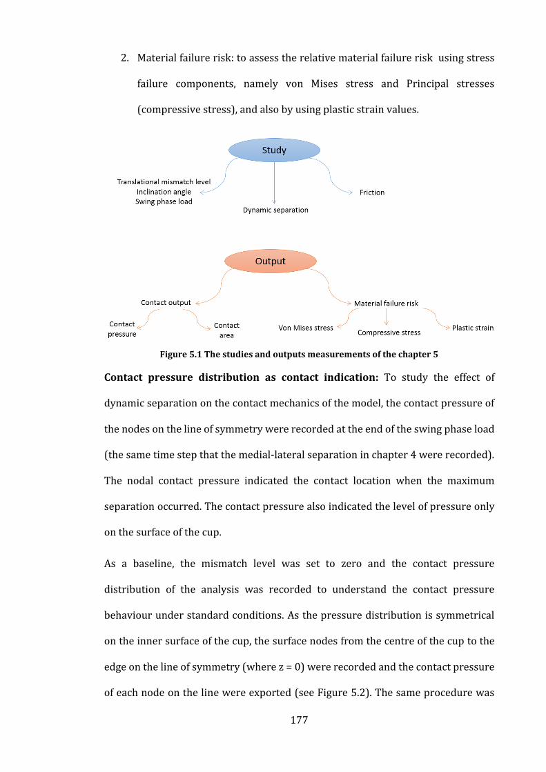
177

2. Material failure risk: to assess the relative material failure risk using stress

failure components, namely von Mises stress and Principal stresses

(compressive stress), and also by using plastic strain values.

Figure 5.1 The studies and outputs measurements of the chapter 5

Contact pressure distribution as contact indication: To study the effect of

dynamic separation on the contact mechanics of the model, the contact pressure of

the nodes on the line of symmetry were recorded at the end of the swing phase load

(the same time step that the medial-lateral separation in chapter 4 were recorded).

The nodal contact pressure indicated the contact location when the maximum

separation occurred. The contact pressure also indicated the level of pressure only

on the surface of the cup.

As a baseline, the mismatch level was set to zero and the contact pressure

distribution of the analysis was recorded to understand the contact pressure

behaviour under standard conditions. As the pressure distribution is symmetrical

on the inner surface of the cup, the surface nodes from the centre of the cup to the

edge on the line of symmetry (where z = 0) were recorded and the contact pressure

of each node on the line were exported (see Figure 5.2). The same procedure was

178

repeated for all the analyses. The node set was equivalent for all the analyses. The

behaviour of the contact pressure is compared between the standard conditions (0

mismatch) and corresponding adverse condition (various mismatches levels). The

input swing phase loads of the compared cases are equal. As Figure 5.2 indicates, to

represent the nodal contact pressure, the nodes are represented as an angle

between the centres of the cup (0°) to the lateral edge where the contact occurs

(96°). Moreover, the contact pressure behaviour throughout the gait cycle is

presented to understand the overall contact behaviour.

Figure 5.2 The nodes on the symmetry line of the contact pressure with respect to the angle from the centre of the line to the lateral edge

Contact area: As the contact area and the applied force are the main factors that

potentially affect the stress and pressure behaviour, it is important to understand

the contact area feedback from the loading and the geometry. The contact area

throughout the gait cycle and at the swing phase load were recorded and presented.

Stress and failure risk analysis: It is important to study the stress behaviour

throughout the gait cycle as the long-term behaviour of UHMWPE can be predicted

by observing the stress behaviour on the cup. There is a large amount of literature

precedent that analyse using a von Mises stresses (e.g. Plank et al., 2005; Hua et al.,

2014). Von Mises stress is used as a representation of the total stress behaviour in

179

all of the directions. It is known as the maximum distortion energy theory of failure,

as it accounts for hydrostatic conditions by including balanced stresses within the

calculation. It is represented as:

𝜎𝑣2 =

1

2⌊(𝜎11 − 𝜎22)2 + (𝜎22 − 𝜎33)2 + (𝜎11 − 𝜎33)2 + 6(𝜎23

2 + 𝜎312 + 𝜎12

2 )⌋

Where σ11 is stress in x direction, σ22 is stress in y direction, σ33 is stress in z

direction, σ23 is shear stress in yz plane, σ31 is shear in zx plane and σ12 is shear in xy

plane. Von mises stress is mostly indication of the shear stress behaviour. If the von

Mises stress on the cup exceeds the elasticity limit, it results in a permanent

deformation of the cup. This failure mode is dependent on the yield point of

UHMWPE and the position and stress level. If a small region on the cup is subject to

some plastic deformation, it affects the material properties of the effected structure

negatively by reducing the elastic modulus, making additional progressive failure

more likely (Hertzberg and Manson, 1980). Such behaviour of plasticity can fatigue

the cup especially during cyclic loading conditions such as walking. For this purpose,

the maximum von Mises stress on the polyethylene cup was calculated.

For each analysis, the maximum von Mises stress at each step during the gait cycle

loading was exported by using a python script (Appendix). Then, the maximum von

Mises stress throughout the cycle was compared in all the cases.

Stress components: The contribution of the maximum principal stress on the stress

behaviour was studied in standard and adverse condition cases as von Mises stress

mostly account the shear stresses involved in the element. Principle stresses are

used to describe phenomena such as the most tensile stress an object experiences

(maximum) and the most compressive stress an object experiences (minimum).

During the gait cycle, the cup liner is compressed against the head as the head and

180

the cup unit are fully fixed. Therefore, the compressive stress can potentially have

an important role in the stress behaviour. As the previous output (von Mises stress

data) indicates the crucial point during the gait cycle. The stress components i.e.,

maximum von Mises stress and compressive stress (minimum principal stress) at

the same data point are compared to understand the principal and shear stress

behaviour on the cup liner.

Plastic Strain: the maximum plastic strain on the cup was recorded for each case to

understand in which analysis permanent material damage occurred. The plastic

strain output is the maximum plastic strain equivalent to the Mises stress. As it was

mentioned, the plastic deformation is a key indication to understand the long-term

material behaviour.

Separation related contact mechanics: The aim of this set of analyses is to

understand the correlation of the dynamic and contact mechanics behaviour of the

THR. In the analyses up to this point, the effect of the parametric sweep is directly

correlated to the contact mechanics output. In this section, the contact mechanics

output are investigated based on the separation corresponded to the parametric

sweep.

Finally, the effect of separation on the contact mechanics was separately

investigated. The same method was used on the analyses that were carried out with

0.1 coefficient friction. The nodal contact pressure of the frictional analyses was

compared to the frictionless analyses. Furthermore, the effect of friction on the

stress components, contact area, and plastic strain is shown.

181

5.3 Results

The output discussed in the methodology section is demonstrated and explained in

this section. The results are presented in the same manner as it was discussed in the

methodology.

5.3.1 Input parameters study

5.3.1.1 Contact output

The contact pressure output is presented into two sections. In this section, the

contact pressure behaviour throughout the gait cycle is first presented. Secondly,

the variation in the contact pressure location and magnitude at the swing phase

under all conditions is described.

5.3.1.1.1 Contact pressure behaviour under all condition

Figure 5.3 represents the nodal contact pressure along the symmetry line in the

0mm to 4mm mismatch levels for various swing phase loads and inclination angles.

As this figure shows, for all mismatch levels, the nodal pressure starts from zero

from the centre to the lateral edge. The nodal pressure increased to the maximum

value and dropped from the peak to zero pressure between the two ends. However,

the distribution and magnitude of the pressure varied between the cases.

In standard conditions, the contact pressure was distributed between 10° to 45° of

the nodal angle and the nodal pressure reached the peak pressure gradually.

However, as the translational mismatch level increased, the nodal pressure

distribution moved towards the lateral edge of the cup more to the point in which

the contact is only at the lateral edge. Higher translational mismatch also affected

the nodal pressure variation. As an example, under 300N swing phase load, nodal

pressure in 4mm mismatch had a substantially higher peak than the rest of the

translational mismatch levels (up to 16MPa) whereas the peak nodal pressure in 0

182

to 3mm cases varied between 8MPa to 9.8MPa in standard condition. Moreover,

under steep cup inclination angle, the peak pressure of even substantially higher

(23.5MPa and 30MPa for 3mm and 4mm, respectively) than the standard cup

inclination angles under 300N swing phase load was observed. The nodal angle

distribution of the cases experiencing higher peak values is lower than the cases that

the pressure variation occurred gradually. Therefore, the maximum pressure

produced under steep cup inclination angle was substantially higher than the

maximum pressure under standard cup inclination angle.

In all the swing phase loads, higher translational mismatch level resulted in a closer

contact pressure distribution to the lateral edge and also it resulted in a

substantially higher peak pressure. However, the occurrence of edge contact

depends on the conditions. The lower swing phase load increased the possibility of

edge contact up to the point that in the analyses with 70N swing phase load, 3 out of

5 cases under standard cup inclination angle and 4 out of 5 cases under steep cup

inclination angle underwent the edge contact with substantially higher peak than

the peak pressure under standard conditions. Furthermore, the effect of steep cup

inclination angle is mostly seen when the edge contact occurred. The steep cup

inclination angle produced a higher pressure peak in the edge contact cases than the

standard cup inclination angle.

183

Figure 5.3 Nodal contact pressure along the line of the symmetry recorded at the end of the swing phase load. Each graph represent the nodal pressure for each swing phase load under standard and steep cup inclination angle. The description of the plots, which is the same for

all graphs, represents the cup inclination angle and the translational mismatch level.

184

5.3.1.1.2 Contact pressure behaviour throughout gait cycle

As an example of the contact pressure changes throughout the gait cycle, the contour

plot of contact pressure throughout gait cycle under 0mm and 4mm translational

mismatch level under 70N swing phase load are represented in Figure 5.4 and

Figure 5.5 signify standard and steep cup inclination angle. Previous chapter also

showed that the separation under 70N swing phase load were higher than any other

swing phase loads. The contour plot of the contact pressure on the cup represent the

pressure variation from minimum of 0Pa (blue) to the maximum value (red). The

conditions with 0mm and 4mm translational mismatch were chosen for

presentation as these two cases result in the minimum and maximum separation

levels (demonstrated in the previous chapter).

It could be seen that under standard cup inclination angle (Figure 5.4), the maximum

contact pressure throughout gait cycle followed the loading changes for both 0mm

and 4mm translational mismatch condition. Although translational mismatch level

increased the maximum contact pressure, the translational mismatch level

produced the most difference in the contact pressure at the swing phase load where

over four times higher contact pressure was produced in the condition with 4mm

translational mismatch level than 0mm translational mismatch level. The contour

plot of the contact pressure at the swing phase load also indicated the edge contact

when translational mismatch level was applied.

185

Figure 5.4 Contact pressure contours and the maximum contact pressure on the liner inner

surface throughout the gait cycle under 45° inclination angle, 70N swing phase load, translational mismatch level of 0 and 4mm

The contact pressure contour plots under steep cup inclination angle produced a

similar trend of contact pressure changes as the standard cup inclination angle.

However, the predicted maximum contact pressure at the swing phase was over five

times higher on the condition with translational mismatch level than the standard

condition. The maximum contact pressure that is produced at the swing phase under

4mm translational mismatch level is only slightly less than the contact pressure that

the cup undergoes at the peak load.

186

Figure 5.5 Contact pressure contours and the maximum contact pressure on the liner inner

surface throughout the gait cycle under 65° inclination angle, 70N swing phase load and translational mismatch level of 0 and 4mm.

5.3.1.1.3 Contact area changes in input parameters

The difference in contact area between the peak and the low load was substantial.

As Table 5.1 represents, the contact area at the peak load varied between 333 mm2

to 354 mm2 under standard cup inclination angle. Moreover, the peak contact area

(that occurs at the peak load) in steep cup inclination angle was less than the peak

contact area under standard cup inclination angle. The peak contact area was more

affected by the cup inclination angle than the swing phase load as the peak contact

area were generally similar in all swing phase loads. The contact area decreased in

swing phase load substantially. In the most severe scenario, the contact area was

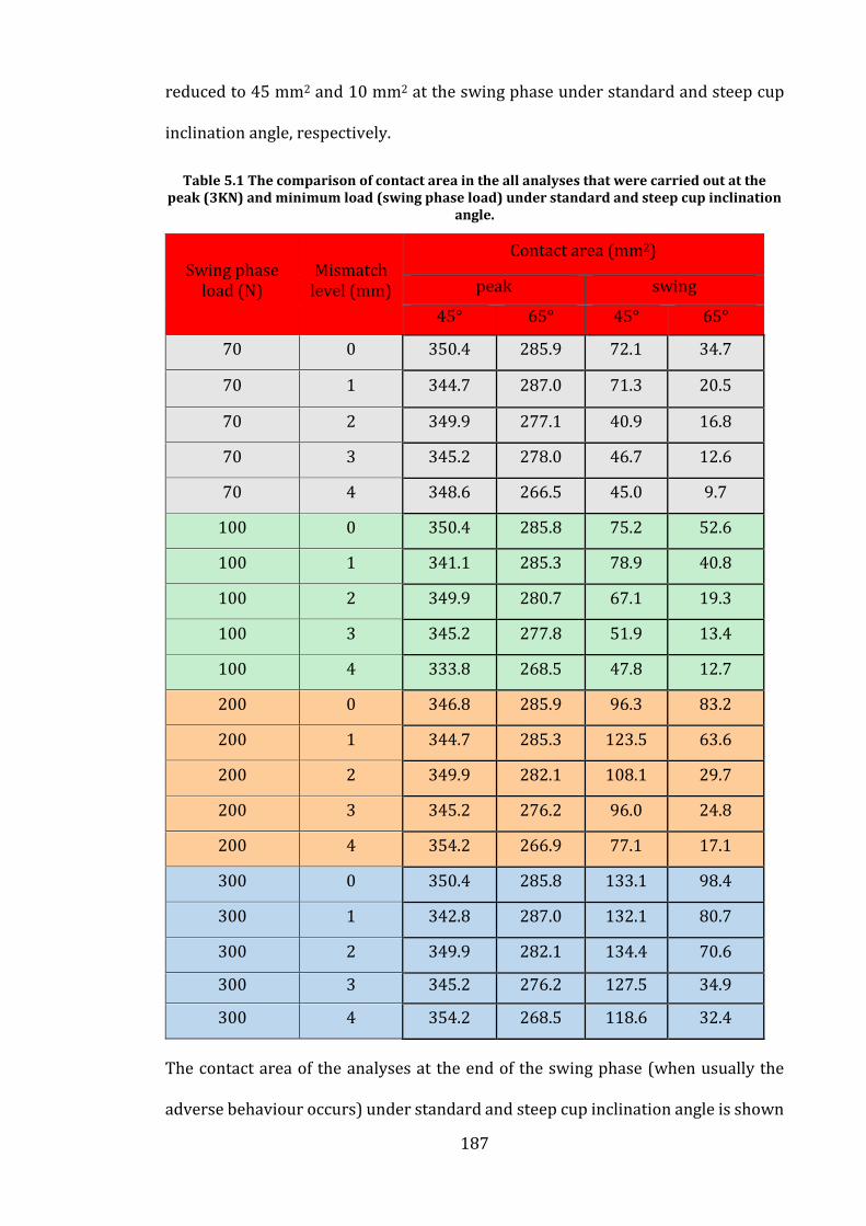
187

reduced to 45 mm2 and 10 mm2 at the swing phase under standard and steep cup

inclination angle, respectively.

Table 5.1 The comparison of contact area in the all analyses that were carried out at the peak (3KN) and minimum load (swing phase load) under standard and steep cup inclination

angle.

The contact area of the analyses at the end of the swing phase (when usually the

adverse behaviour occurs) under standard and steep cup inclination angle is shown


Mismatch level (mm)

Contact area (mm2)

peak swing

45° 65° 45° 65°

70 0 350.4 285.9 72.1 34.7

70 1 344.7 287.0 71.3 20.5

70 2 349.9 277.1 40.9 16.8

70 3 345.2 278.0 46.7 12.6

70 4 348.6 266.5 45.0 9.7

100 0 350.4 285.8 75.2 52.6

100 1 341.1 285.3 78.9 40.8

100 2 349.9 280.7 67.1 19.3

100 3 345.2 277.8 51.9 13.4

100 4 333.8 268.5 47.8 12.7

200 0 346.8 285.9 96.3 83.2

200 1 344.7 285.3 123.5 63.6

200 2 349.9 282.1 108.1 29.7

200 3 345.2 276.2 96.0 24.8

200 4 354.2 266.9 77.1 17.1

300 0 350.4 285.8 133.1 98.4

300 1 342.8 287.0 132.1 80.7

300 2 349.9 282.1 134.4 70.6

300 3 345.2 276.2 127.5 34.9

300 4 354.2 268.5 118.6 32.4

188

in Figure 5.6. Generally, the contact area decreased as the translational mismatch

level increased in all the conditions except 70N swing phase load and steep cup

inclination angle where the contact area slightly increased between 2mm and 3mm

translational mismatch level. In standard cup inclination angle the contact area

varied between 135 mm2 to 45 mm2. However, the contact area for all the cases

dramatically decreases in steep cup inclination angle. The contact area variation

under steep cup inclination angle is between 80 mm2 to 10mm2.

Figure 5.6 The contact area at the end of the swing phase load for various translational mismatch level and swing phase loads. The contact area of the analyses under standard and

steep cup inclination angle are plotted as 'standard' and 'steep', respectively

5.3.2 Material failure risk

5.3.2.1 Von Mises stress throughout the gait cycle

Figure 5.7 represents the maximum stress behaviour during gait cycle in the

concentric condition analyses (0 mismatch level) under 45° and 65° inclination

angle and variation of swing phase loads. The overall stress behaviour follow the

axial loading behaviour in all of the swing phase loads variations for all the cases.

The largest difference between the cases occurred during the swing phase. Higher

swing phase load resulted in a higher stress during the swing phase for both cup

0

20

40

60

80

100

120

140

160

0 0.5 1 1.5 2 2.5 3 3.5 4 4.5

Co

nta

ct a

rea

(mm

2 )


Standard, 70N Standard, 100N Standard 200N Standard, 300N

Steep, 70N Steep, 100N Steep, 200N Steep, 300N

189

inclination angles. Moreover, the steep cup inclination angle resulted in a lower

stress value throughout the gait cycle in all swing phase loads.

Figure 5.7 Stress distribution of the analysis with 0 mismatch level under 45° inclination angle (solid lines) and 65° inclination angle (dotted lines) with swing phase load of 70N to

300N

The ‘in cycle’ stress behaviour is observed to either follow the loading trend or

produce a higher level of stress during swing phase load (adverse stress behaviour).

However, as the swing phase load decreased the number of the conditions that

produce adverse stress behaviour during swing phase increased in both standard

and steep cup inclination angle (Figure 5.8). The cup underwent the adverse stress

behaviour and the maximum stress value that is produced at the swing phase load

decreased by decreasing the swing phase load. Since there is an axial loading

(equivalent to the swing phase load of the analysis) during stabilisation step which

occurs before gait cycle loading, the initial stress at the gait cycle is not zero.

When 300N swing phase load was applied, there is a similar stress behaviour in the

analyses with 1mm, 2mm and 3mm mismatch level that followed the loading

0

2

4

6

8

10

12

14

0 0.2 0.4 0.6 0.8 1 1.2

Max

vo

n m

ises

str

ess

(MP

a)

Time (s)

70N, 45 degree inclination 100N, 45 degree inclination

200N, 45 inclination angle 300N, 45 degree inclination

70N, 65 degree inclination 100N, 65 inclination angle

200N, 65 degree inclination 300N, 65 degree inclination

190

changes under standard cup inclination angle. In the mentioned conditions

translational mismatch level and the maximum stress was initiated and finished (at

the swing phase load) at the value of 4.4MPa, 4MPa and 5.2MPa, respectively. Out of

all of the cases that are demonstrated with 300N swing phase load and standard cup

inclination angle, the analysis with 4mm mismatch level had a dissimilar behaviour.

In this analysis, the stress behaviour was initiated with a substantially higher stress

value of 10MPa. The stress behaviour during the stance phase was similar to the rest

of the cases. However, during swing phase, the maximum stress initially decreased

from 12.3MPa (the peak stress) to 6MPa then a moderate increase of maximum

stress to 10MPa occurred. After the increase in the stress value during the swing

phase load, the maximum stress becomes constant until the end of the swing phase

load.

191

Figure 5.8 The maximum von Mises stress throughout the gait cycle for all of the conditions. The dashed line plots represent steep cup inclination angle and the solid line plots represent

standard cup inclination angle at different mismatch level

A similar trend of stress variation was seen in analyses under steep cup inclination

angle for 300N swing phase load. However, the only condition that followed the

192

loading changes under steep cup inclination angle was the analysis with 1mm

translational mismatch level. The rest of the analysis resulted in a higher stress level

during swing phase load than expected. The conditions that resulted in a higher

stress value during swing phase load also experienced higher stress value at the

beginning of the cycle. Moreover, in all of the cases, steeper cup inclination angle

produced higher stress at the swing phase load than the standard cup inclination

angle.

The contour plot of the von Mises stress at the swing phase load under standard cup

inclination angle is shown in Figure 5.9. The contour plot showed the stress

distribution on the cross section area where the thickness of the cup is. In all the

analyses, the same contour limit is used for a simpler comparison. In the same swing

phase load, the stress distribution moved to the lateral edge of the cup by the

increase in translational mismatch level. Moreover, higher swing phase load

increased the stress value in the thickness of the cup.

193

Figure 5.9 The cross sectional contour of von Mises stress at the end of swing phase load under standard cup inclination angle for the analyses with swing phase load of 70N to 300N

and translational mismatch level of 0mm to 4mm.

Figure 5.10 represents the cross sectional contour of von Mises stress at the end of

swing phase load under standard cup inclination angle. A similar trend can be seen

in the steep cup inclination angle. Although, the stress distribution moved towards

the edge by higher translational mismatch level, the stress distribution in standard

condition is closer to the edge than the stress distribution in steep cup inclination

angle which caused higher number of edge contact out of all the analyses.

Furthermore, higher stress values were recorded for steeper cup inclination angle.

194

Figure 5.10 The cross sectional contour of von Mises stress at the end of swing phase load under steep cup inclination angle for the analyses with swing phase load of 70N to 300N and

translational mismatch level of 0mm to 4mm.

5.3.2.2 Maximum principal stress at swing phase load

Figure 5.11 shows the maximum compressive stress and the von Mises stress

increased as the translational mismatch increases. Also, higher swing phase load

resulted in higher stress values (both values) in a specific translational mismatch

level condition. However, this trend could not be seen in the compressive stress of

the conditions with 70N swing phase load. Furthermore, the maximum compressive

stress at the swing phase load is substantially higher than the von Mises stress

195

values in most of the conditions. The only condition that the compressive stress is

slightly higher than the von Mises stress is the one with 70N swing phase load and

4mm translational mismatch level.

Figure 5.11 Comparison of the maximum compressive stress and von Mises stress under standard cup inclination angle translational mismatch levels of 0mm to 4mm

Figure 5.12 focuses on the compressive and von Mises stress of the analyses that

were carried out under steep cup inclination angle. This figure agreed that the both

stress types increased as the translational mismatch and swing phase load

increased. The compressive stress that was produced was also notably higher than

von Mises stress. The only condition that disagreed with the higher compressive

stress than the von Mises stress outcome is the analysis with 100N swing phase load

and 4mm translational mismatch level.

0

5

10

15

20

25

0 0.5 1 1.5 2 2.5 3 3.5 4 4.5

Stre

ss (

MP

a)


Compressive stress 300N Von Mises stress 300N Compressive stress 200N

Von mises stress 200N Compressive stress 100N Von mises stress 100N

Compressive stress 70N Von mises stress 70N

196

Figure 5.12 Comparison of maximum compressive stress and von Mises stress under steep cup inclination angle and translational mismatch levels of 0mm to 4mm

5.3.2.3 Plastic strain

No plastic strain was recorded when 300N swing phase load or 1mm mismatch level

was applied (Figure 5.13). 200N swing phase load caused a plastic strain only when

4mm mismatch was applied. A level of plastic strain was recorded in 100N swing

phase with 3mm and 4mm mismatch. The cases with most plastic strain occurrence

is 70N swing phase load.

0

5

10

15

20

25

30

0 0.5 1 1.5 2 2.5 3 3.5 4 4.5

Stre

ss (

MP

a)


Compressive stress 300N Von Mises stress 300N Compressive stress 200N

Von mises stress 200N Compressive stress 100N Von mises stress 100N

Compressive stress 70N Von mises stress

197

Figure 5.13 Maximum plastic strain in the cases with various translational mismatch level and swing phase loads under 45° inclination angle

Figure 5.14 demonstrates the plastic strain data exported under steep cup

inclination angle. Once more, no plastic strain was recorded in 1mm mismatch level.

In the cases with 3mm and 4mm mismatch level, occurrence of plastic strain was

observed for all the swing phase loads and the only case that did not affect the plastic

strain in 2mm mismatch level was 300N swing phase load. Therefore, the number

of cases that the plastic strain occurred in, is higher in the cup inclination of 65° than

45°.

0

0.01

0.02

0.03

0.04

0.05

0.06

0.07

0.08

0.09

1 2 3 4

Pla

stic

str

ain

Separation (mm)

70N 100N 200N 300N

198

Figure 5.14 Maximum plastic strain in the cases with 65° inclination angle and all of the swing phase loads and translational mismatch levels

5.3.2.4 Contact area as driven for stress behaviour

Furthermore, it was shown in chapter 4 that there is a substantial load at the rim at

the beginning of the stance phase. The high load at the rim was used as a reason for

high wear rate when edge loading occurs. However, the stress behaviour indicated

that the contact area increased substantially in the first 0.5s of the gait cycle which

did not lead to high stress and potentially the most crucial damage zone

(Figure 5.15). Although the load and contact area increased, the stress behaviour

from the beginning of stance phase to the first peak load showed a decrease in the

level of stress due to the substantial contact area increase. The contact area at 0.5s

of the gait cycle was 320 mm2 whereas the contact area at the beginning of the stance

phase depended on the swing phase load (48mm2 for 70N swing phase load to

125mm2 for 300N swing phase load). Then, the contact areas changes between the

0.5s to the peak load is moderate and consequently, the stress increased moderately

in the same time frame.

0

0.01

0.02

0.03

0.04

0.05

0.06

0.07

0.08

0.09

0.1

1 2 3 4

Pla

stic

str

ain

Separation (mm)

70N 100N 200N 300N

199

Figure 5.15 Contact area and von Mises stress versus time in the analyses with 4mm translational mismatch level, various swing phase loads and standard cup inclination angle

The corresponding contact area to the stress initialisation under steep cup

inclination angle is shown by a black line in Figure 5.16. The value of corresponding

contact area is less in steep cup inclination angle than the standard cup inclination

angle. The variation of the contact area is between 55 mm2 and 85 mm2. The point

in which the adverse stress initiated from is similar in both standard and steep cup

inclination angle (0.65s). The similar trend between the contact area and the stress

behaviour was observed under standard cup inclination angle at the beginning of

stance phase up to the first peak load. However, the changes of contact area in the

first 0.5s of the gait cycle is greater in steep cup inclination angle than the standard

cup inclination angle as the contact area at the beginning of stance phase was under

50 mm2 for all swing phase loads.

0

2

4

6

8

10

12

14

16

0

50

100

150

200

250

300

350

400

0 0.1 0.2 0.3 0.4 0.5 0.6 0.7 0.8 0.9 1

Vo

n m

ises

str

ess

(MP

a)

Co

nta

ct a

rea

(mm

2 )

Time (s) Contact area, 300N Contact area, 200N Contact area, 100N Contact area, 70N

Stress, 300N Stress, 200N Stress, 100N Stress, 70N

200

Figure 5.16 Contact area and von Mises stress versus time in the analyses with 4mm translational mismatch level, various swing phase loads and steep cup inclination angle.

5.3.3 Separation study

The relationship between the separation and the contact area resulted from the

separation is shown in Figure 5.17. The contact area derived from the separation

under 0.5mm varied especially in standard cup inclination angle. As it was defined

in Chapter 4, the separation under 0.5mm doesn’t result in edge loading. In both cup

inclination angles, the contact area generally decreased as the separation increased

(for over 0.5mm separations). However, the pattern of decreasing contact area (for

separation higher than 0.5mm) can be clearly seen for the analyses under standard

condition, and not in other conditions.

0

2

4

6

8

10

12

14

16

0

50

100

150

200

250

300

0 0.1 0.2 0.3 0.4 0.5 0.6 0.7 0.8 0.9 1

Stre

ss (

MP

a)

Co

nta

ct a

rea

(mm

)

Time (s)

Contact area, 300N Contact area, 200N Contact area, 100N Contact area, 70N

Stress, 300N Stress, 200N Stress, 100N Stress, 70N

201

Figure 5.17 Contact area at the maximum separation during the gait cycle under standard and steep cup inclination angle with all translational mismatch levels and swing phase loads.

The other contact mechanics data such as contact pressure, compressive stress and

von Mises stress cannot directly be compared to the separation value regardless of

the condition taken as the swing phase load (Figure 5.18) and the translational

mismatch level (consequently M/L force) affected these data. However, if the

conditions are taken into consideration, higher translational mismatch level and

higher swing phase load (in isolation) increased the maximum Von Mises stress,

compressive stress and contact pressure. Moreover, it could be seen that the

separation higher than 0.5mm also affect the mentioned parameters.

0

20

40

60

80

100

120

140

160

0 0.5 1 1.5 2 2.5 3 3.5 4

Co

nta

ct a

rea

(mm

2 )

Separation (mm)

Standard cup inclination angle Steep cup inclination angle

202

Figure 5.18 The comparison of separation with von Mises stress, compressive stress and contact pressure. The analyses under standard cup inclination angle are presented as Plot A and the analyses under steep cup inclination angle is presented as Plot B

203

As Figure 5.19 represent, the plastic strain is initiated when the separation is higher

than 0.6mm and 0.7mm in standard and steep cup inclination angle, respectively. The

level of plastic strain increases as the separation level increases. In standard cup

inclination angle, a linear relationship between separation and plastic was observed.

However, the similar trend cannot be concluded in the analyses under steep cup

inclination angle.

Figure 5.19 The comparison of separation with plastic strain for both standard and steep cup inclination angles with all translational mismatch levels and swing phase loads.

5.3.4 Friction

The effect of friction on contact mechanics was analysed. Figure 5.20 represents the

nodal pressure along the line of symmetry with 0.1 coefficient of friction and no friction

under steep cup inclination angle and various swing phase loads. The comparison of

the two analyses only indicated a similar nodal pressure distribution position in 70N

swing phase load and slightly different distribution in 300N swing phase load. However,

204

a difference in the peak nodal pressure was seen (4MPa difference). Moreover, the

frictional analysis only increased the peak contact pressure in lower swing phase load

(70N).

Figure 5.20 Effect of friction on the contact pressure along symmetrical line under standard cup inclination angle, 300N and 70N swing phase load and 4mm translational mismatch level.

The frictional analyses that were carried out under steep cup inclination angle resulted

in the similar outcome in distribution (Figure 5.21). The correlation between the peak

contact pressure and the swing phase load in the frictional and frictionless analyses was

similar. In both swing phase loads, the friction between the contact surfaces decreased

the peak contact pressure under steep cup inclination angle.

0

5

10

15

20

25

0 20 40 60 80 100 120

Co

nta

ct p

ress

ure

(M

Pa)

Angle

Frictional, 300N frictionless, 300N Frictional, 70N Frictionless, 70N

205

Figure 5.21 Effect of friction on contact pressure along the symmetrical line under steep cup inclination angle, 300N and 70N swing phase load and 4mm translational mismatch level.

Figure 5.22 represents the changes in the stress behaviour between the frictional and

frictionless contact against the loading cycle in the analyses under standard cup

inclination angle. Overall, the friction affected the stress changes during stance phase

between two peaks for both conditions. However, the effect of friction on the stress

during swing phase load was dependant on the swing phase load value. Lower stress

value was found in the frictional analysis than the frictionless one whereas the lower

swing phase load generated a higher stress during swing phase load than the

frictionless analysis.

0

5

10

15

20

25

30

35

0 20 40 60 80 100 120

Co

nta

ct p

ress

ure

(M

Pa)

Angle(°) Frictional, 300N frictionless, 300N Frictional, 70N Frictionless, 70N

206

Figure 5.22 Effect of friction on the analyses under standard cup inclination angle with the lowest (70N) and highest (300N) swing phase load. The figure represents the effect of friction on

the von Mises stress during a gait cycle.

The similar trend of the friction effect under standard condition was observed

(Figure 5.23) in the analyses under steep cup inclination angle. Lower swing phase load

negatively affected the stress values during the swing phase load under steep cup

inclination angle.

Figure 5.23 Effect of friction on the analyses under steep cup inclination angle with the lowest (70N) and highest (300N) swing phase load. The figure represents the effect of friction on the

von Mises stress during a gait cycle.

0

2

4

6

8

10

12

14

16

0 0.2 0.4 0.6 0.8 1

Vo

n m

ises

str

ess

(MP

a)

Time (s)

Friction, 300N Friction, 70N Frictionless, 300N Frictionless, 70N

0

5

10

15

20

25

0 0.2 0.4 0.6 0.8 1

Vo

n m

ises

str

ess

(MP

a)

Time (s)Friction, 300N Friction, 70N Frictionless, 300N Frictionless. 70N

207

The friction had little effect on the compressive stress under steep cup inclination angle

(Figure 5.24). However, conflicting results on the compressive stress was observed in

different swing phase loads under standard cup inclination angle. Comparison of the

frictional and frictionless analysis indicates that friction in low inclination angle

resulted in a reduction in the compressive stress whereas higher swing phase load

caused an increase in the compressive stress.

Figure 5.24 The effect of friction on the compressive stress of the analyses. The friction coefficient of 0.1 was applied on the lowest (70N) and highest (300N) swing phase load and on

the standard and steep cup inclination angle.

Friction affected the contact area at the swing phase load and the magnitude of this

effect depend on the cup inclination angle. As Figure 5.25 represents, friction decreased

the contact area slightly in the steep cup inclination angle analyses. Although the

friction effect on the contact area is not substantial, the reduction in contact area was

more noticeable in standard cup inclination angle.

0

5

10

15

20

25

30

300 70

Max

Co

mp

ress

ive

stre

ss (

MP

a)


Frictional, steep Frictionless, steep Frictional, standard Frictionless, standard

208

Figure 5.25 The comparison of the contact area in the frictional and frictionless analyses. The friction coefficient of 0.1 was applied on the lowest (70N) and highest (300N) swing phase load

and on the standard and steep cup inclination angle.

Although, friction slightly decreased the plastic strain of the conditions that were

analysed, no substantial difference in plastic strain was observed for any of the cases

(Figure 5.26).

Figure 5.26 The effect of friction on the plastic strain on the lowest (70N) and the highest (300N) swing phase load with 4mm translational mismatch level and on the standard and steep cup

inclination angle.

0

20

40

60

80

100

120

140

300 70

Co

nta

ct a

rea

(mm

2 )


Frictional, Standard Frictionless, standard Frictional, Steep Frictionless, steep

0

0.01

0.02

0.03

0.04

0.05

0.06

0.07

0.08

0.09

0.1

300 70

Pla

stic

str

ain


Frictional, standard Frictionless, standard Frictional, steep Frictionless, steep

209

5.4 Discussion

Dynamic modelling of a THR under a load cycle provides a unique opportunity to

predict and analyse the effect of various parameters describing the contact mechanics

of the joint. These contact mechanics analyses produced a novel insight to understand

the potential damage, fatigue and wear of the contact surfaces throughout the gait cycle

under adverse conditions.

5.4.1 Contact behaviour due to the input parameters

The pressure distribution in various mismatch levels indicated that the standard

condition resulted in a concentric head and cup contact. The highest mismatch level

caused the closest contact to the lateral edge in all the swing phase loads. Deviation

from contact concentricity caused edge contact and therefore a substantially reduced

contact area. The result of smaller contact area was a substantially higher localized

contact pressure towards the edge. The highly localised pressure distribution, which

could be an indication of the most damaged area, is observed more when the swing

phase load is 70N, or 100N as compared to the 200N and 300N cases.

The comparison of the contact pressure behaviour in mismatch level variation for

standard and steep cup inclination angle indicated that the edge contact pressure

behaviour was observed in a greater number of cases when the cup inclination angle

was steeper than standard cup inclination angle. The horizontal distance between the

centre and the edge of the cup is less in the steep cup inclination angle cases than

standard inclination angle cases due to lateral cup edge location. Consequently, the

edge contact is more frequent in the cases with steeper cup inclination angle and the

edge wear damage could potentially be higher for these cases.

210

5.4.2 Discussion of stress behaviour throughout gait cycle

Contact mechanics analysis within the gait cycle was also studied based on the level of

stress that the cup undergoes. In the standard conditions, the stress variation followed

the loading changes throughout the gait cycle. In the adverse conditions, edge loading

and permanent deformation are multifactorial scenario occurrences and the effect of

each input parameter is challenging to identify. Higher translational mismatch, steeper

cup inclination angle and lower swing phase load all increased the separation level and

occurrence of edge loading (Figure 5.27). A similar trend was observed in contact

mechanics output.

Figure 5.27 The correlation between the input parameters and edge loading, adverse stress

behaviour and plastic strain occurrence. The green, yellow and orange cells represent the edge loading, adverse stress and plastic strain occurrence for various swing phase loads, respectively

The stress behaviour during the stance phase is dictated by the loading however the

stress behaviour during the swing phase is affected by various factors. During swing

phase, in some cases, the maximum stress initially decreases, increases and then

becomes constant. There are two factors that contribute to such stress behaviour:

211

1) The resultant force that is influenced by both the swing phase load (axial load) and

the translational mismatch level which affects the medial-lateral force (by varying

the compression of the spring). As the axial load decreased to the swing phase load,

the contact area moved towards the edge of the cup. However, the contact area is

still in the ‘safe support zone’ to the point that the stress level is decreased to the

minimum. This suggests that up to this point of the cycle changes in contact area are

negligible, so the decrease in stress level corresponded to the decrease in axial

loading. After this point of the cycle, the contact area started being in the ‘crucial

region’ where the contact area became significantly smaller. Consequently, the

stress raised again as the axial loading is constant. The lower swing phase load and

the higher translational mismatch level drives the cup towards the lateral edge

where the contact zone was significantly smaller.

2) The cup inclination angle plays an important role in the contact zone as the location

of the lateral edge varied by the inclination angle. It was described that the travelling

distance of the head to the lateral cup edge is less in steeper cup inclination angle

(Chapter 4). Under steep cup inclination angle, the translational mismatch level of

3mm and 4mm caused permanent deformation regardless of the swing phase load.

The permanent deformation for the same translational mismatch levels (3mm and

4mm) under standard cup inclination angle did not occur under higher swing phase

load than 200N. In the standard cup inclination angle case the larger contact area

associated with the 45 cup inclination angle reduced the severity of the contact

mechanics, such as stress and permanent deformation, due to the location of the

lateral edge and the resistance to the lateral movement.

212

Although a high load level was observed on the rim at the beginning of stance phase

where the separation was greater than 0.5mm, no substantial contact output such as

stress level was observed during this time duration. The stress level actually decreased

initially as the contact area increased dramatically from the start of the stance phase to

the first peak load. Therefore, most of the load is distributed in the higher contact area

and the higher contact area potentially overcame the high load on the rim.

The initial and final stress behaviour of each cases in adverse conditions seemed to be

similar. In fact, in some of the conditions with the 4mm mismatch level, the stress value

is initiated in a substantially higher value that caused an unexpected stress variation as

the axial load reached its first peak. In the extreme conditions, the initial stress value is

higher than the stress generated at the peak load due to the changing contact area. As

the load increased rapidly to the first peak, it could have a significant impact on the cup

material behaviour due to the rapid sliding and the high stress values.

Dynamic modelling enabled the analysis of the time that the THR is under adverse

loading conditions as a proportion of the total time for one cycle. The maximum von

Mises stress throughout the gait cycle indicated that the area in which the adverse

stress level occurred experienced this stress for over 35% of the gait cycle. Moreover,

the severity of the adverse stress behaviour is affected by the level of input parameters.

From a failure perspective, it could be concluded that under the cyclic loading, the

conditions that show a higher severity of the adverse stress behaviour are likely to have

a greater risk of earlier failure due to the large stress level within the zone.

213

5.4.3 Failure Prediction

There are a number of failure theories such as shear strain energy theory (von Mises)

and maximum principal stress theory that are applicable for ductile or brittle materials.

In FE packages, the input yield stress is based on the von Mises stress value. Therefore

the von Mises stress failure criterion has been used as the failure prediction in many

previous studies (Mak and Jin, 2002; Korhonen et al., 2005; Hua et al., 2014). If the von

Mises stress in the model exceeds the yield stress, permanent deformation of the

material occurs. When this is applied to THR, after the yield stress is reached the

material deforms permanently and changes the shape of the edge of the cup. The von

Mises stress reported by the model after the failure can be unreliable, as the properties

of the deformed component have changed and Hooks law no longer applies. Von Mises

stress is predominantly driven by shear stresses, however it still consider the principal

stress within the calculation. It was shown that the maximum compressive stress is

substantially higher than the value of the von Mises stress in all the conditions which

indicates the compressive stress dominated the stress behaviour. There may be an

argument to consider other failure theories for this reason.

One of the main reason for UHMWPE failure in THR is reported to be fatigue (Kurtz,

2004; Partridge, 2016). Fatigue damage is caused by repeated cyclic loading that is not

fully considered in this study. However, some predictions can be made based on the

overall stress behaviour. The higher plastic strain was observed more for the conditions

with higher edge loading and due to the high concentrated stress in the edge area.

Further cyclic loading is expected to weaken the material properties in this region and

potentially cause a failure below the yield stress. With a single cycle the type and

214

severity of failure cannot be predicted. However, the model predicts a high stress from

the centre of the cup to the lateral edge. Therefore, this is assumed to be the main area

of the damage, and experimental data showed increased wear and deformation in this

region. The worn and damaged area on the cup that is shown in Figure 5.28 is for the

experimental testing under 70N swing phase load. Figure 5.28 indicated that the higher

translational level and steeper cup inclination angle firstly increases the level of

deformation and wear, and secondly affected the lateral edge of the cup. Although it is

not possible to distinguish between the level of wear and deformation in the

experimental study, higher translational mismatch and/or steeper cup inclination

angles increases the stress on the edge which would be expected to cause more damage

over time. The direct comparison of the experimental and computational damage for

this specific swing phase load (70N) is a challenging task as the computational study

shows higher separation level (Chapter 4) than the experimental study which can

directly affect the stress concentration and consequently the predicted damaged area.

Figure 5.28 The worn and deformed area of the UHMWPE cup under 0mm, 2mm and 4mm translational mismatch level, standard and steep cup inclination angle and 70N swing phase

load. The worn area indicates the worn and deformation on the inner surface of the liner (Appendix)

215

5.4.4 The correlation between separation and contact mechanics

The analyses all indicated higher level of separation resulted in higher stress, contact

area and plastic strain values. This conclusion is supported by a previous study on the

effect of dynamic separation on the contact mechanics of THR statically (Hua et al.,

2014). However, their static FE model studied a lower level of separation than this

study. The correlation between the separation and contact mechanics was investigated

and it was indicated that the contact area at the swing phase load decreased

substantially when the separation level was higher than 0.5mm under standard cup

inclination angle. However, the border of the separation level for higher contact area

was slightly less (0.4mm) under steep cup inclination angle. A similar trend was seen

between the separation level and the stress values. This indicated the dynamic

separation that is required to noticeably affect the contact mechanics output is less in

the steep cup inclination angle. The higher occurrence of plastic strain in the 65 cup

inclination angle supported the conclusion that more cases are potentially damaged

under comparable conditions.

5.4.5 Friction effect

The effect of friction was highest when the contact mechanics of standard cup

inclination angle and lower swing phase load were observed. The stress level, contact

pressure and plastic strain all increased when friction was added into the model. The

high M/L load in 70N condition drove the contact area towards the edge of the cup,

where the geometry of the edge under the standard cup inclination angle forms a

locking mechanism (compared to the steeper cup inclination angle where the lateral

movement is easier) and a resistance to the movement to the edge. Furthermore, the

216

resistance force formed by the friction affected the stress level on standard cup

inclination angle with low swing phase load condition more than the other conditions

tested. Friction did not play an important role in terms of the dynamic output of the

model (separation). However, the contact mechanics of the model can be altered by the

friction in the bearing surfaces.

5.4.6 Model improvements

It was shown in the previous chapter that the developed model is sensitive to the input

parameters under dynamic conditions. The contact mechanics studies of the model also

indicate that the variation in input parameters affects the contact behaviours, as

hypothesised. However, this developed model could be improved for a more efficient

and accurate contact output. As an example, no mesh sensitivity analysis was carried

out when edge loading occurred as the mesh sensitivity was done under standard

condition during the model development. Therefore, a change of the value of the contact

mechanics output could be expected if this were implemented. However, the trend of

the contact changes is not expected to change as the same meshing ratio was configured

for all the conditions. Moreover, as presented in chapter 2, the output was not affected

by the refinement when the same meshing ratio on both contact surfaces was created.

Therefore, as the same meshing ratio is applied to the contact surfaces in all models,

only slight changes in the magnitude of the outputs is expected.

In FE modelling, the material model plays a very important role in contact mechanics

behaviour. In this study the material behaviour is assumed to be elastic-plastic and this

material behaviour is used in the THR model previously (Hua et al., 2014), however,

this material model is mostly suitable for metals that have insubstantial plastic strains.

217

There are previous studies investigating the most suitable material for modelling

UHMWPE and it was concluded that the hybrid material model can predict the

UHMWPE behaviour more accurately than elastic-plastic model (Bergström, Rimnac

and Kurtz, 2005). Furthermore, it was shown the hybrid material model can predict

failure methods by using chain stretch theory, which studies the breakage of the

polymer chains in the material. Therefore, if a hybrid material model is assigned to the

UHMWPE, better predictions of the contact mechanics can be made. However, the effect

of the hybrid material model on the running time and efficiency of the FEA should be

examined.

5.5 Key points

As the experimental and computational simulations both propose an agreement in

dynamic and contact mechanics outcomes, it could be concluded that the developed

methodology could be a great tool to predict the device sensibility under various

conditions.

The contact mechanics behaviour is dependent on the following combination of

parameters: geometric changes caused by changes in cup inclination angle; and the

resultant force on the cup, which is affected by the swing phase load and the

translational mismatch level.

Higher translational mismatch level, lower swing phase load and steeper cup

inclination angle resulted in a reduced contact area, higher adverse stress

occurrence and higher permanent deformation on the edge of the cup.

218

The THR is better to be implanted in the standard cup inclination angle as the

indications of the damage were observed in the steep cup inclination angle

conditions.

219

Chapter 6 Final discussion and future work

This chapter focuses on the overall model development, the potential consequences and

the limitations of the developed method. Furthermore, the possible application of this

method in the future is described.

6.1 Model development

The ultimate aim of this project was to develop a computational model to

simultaneously compute the dynamic and contact mechanics of the THR under adverse

conditions. The developed model can analyse dynamic contact mechanics patterns

throughout the gait cycle, which would be impossible using current static modelling

techniques. The immediate implication of this is the ability to study how the separation

is driven dynamically by the effect of external factors. Additionally, the contact

mechanics can be studied concurrently. This computational model can be used as a tool

to complement experimental observations and provide data that is unavailable

experimentally, such as the THR contact mechanics behaviour throughout one loading

cycle, resulting in analysis through various load and contact conditions. With some

additional development, this computational model could be modified to suit the

applications within research, industry or as a preoperative tool.

The development of explicit THR models is challenging as it has not been explored until

recently for use in preclinical testing. The integration of the dynamic and contact

mechanics under adverse conditions can cause model instability as a result of edge

loading. Therefore, it was important to first build a basic model and then gradually add

sophistication such as loading profiles and detailed geometry.

220

The model was set to mimic a station of Leeds II hip simulator that has been used to

examine THR wear characteristics under adverse conditions (Al-Hajjar et al, 2010). The

development is fully described in Chapters 2 and 3. Not all the experimental aspects of

this simulator are necessary to replicate the separation or the contact mechanics, so

some assumptions and simplifications can be made to reduce the time of the analysis,

increase the model reliability, and aid troubleshooting. The most crucial experimental

component that was implemented into the computational model was the spring, which

created the separation between the contact surfaces. The spring has a major effect on

the outputs and oscillations in the model and one of the challenges was to ensure

appropriate damping for specific cases, as each of the input factors and their

interactions affected those damping conditions.

The next step of the development was the validation of the in silico dynamic outputs

against the in vitro studies. The comparison demonstrated similar levels of separation

and contact mechanics changes in both experimental studies and computational

models. However, future modifications of this model could potentially provide a more

reliable outcome compared to the experimental studies as will be discussed below.

Furthermore, the validation of the dynamic data increases the reliability of the contact

mechanics outputs as the contact mechanics related parameters cannot be measured

directly from in vitro studies.

The advanced developments of the model could be dependent on the applications of it.

The current model mimics the general THR behaviour of the in vitro loading, geometry

and positioning of the stations of the hip simulators. Therefore, if the outcome of

interest is the overall THR in vitro performance under numerous conditions, the

computational model inputs can be based on the experimental set up. If the model is

221

used to study the effect of other factors on the THR performance, then the modifications

can be done on the model that is already developed. In addition, if the model was used

to study patient specific outputs, then the patient’s data such as the bone anatomy, axial

loading and tissue behaviour would also need to be implemented in the model for a

more realistic output. It should be noted it is currently challenging to discover the

patient’s specific data as there are not many patient related data sets published due to

the difficulty in measuring the patient’s data.

Implementation of an anterior-posterior spring to mimic various hip tissues behaviour

could be the next step to replicate a more in vivo representative situation in the

computational model. The hip joint is supported well by iliofemoral, pubofemoral, and

ischiofemoral ligaments and they are surrounded by rectus femoris muscles for better

stability (Tortora and Nielsen, 2009). The anterior-posterior spring could be a useful

tool to implement different soft-tissue scenarios.

6.2 Discussion of findings The dynamic behaviour and contact mechanics of the CoP THR under adverse

conditions were analysed in Chapters 4 and 5. It was concluded from the analyses that

a higher translational mismatch level, steeper cup inclination angle and lower swing

phase load could all increase the dynamic separation. The same trend was seen in

experimental studies (Ali et al., 2016). However, the magnitude of the dynamic output

was not always similar which could be due to the various reasons such as damping

conditions, friction and angular movements. The computational model clearly

distinguished the effect of each input on the model dynamically. Therefore, the model

can be used to understand the effect of variety of parameters on the dynamic aspect of

the model.

222

A similar trend to the separation was seen in stress behaviour on the cup. If the adverse

conditions caused dynamic separation of more than 0.5mm in the standard cup

inclination angle condition or 0.4mm in the steep cup inclination angle condition, then

an adverse ‘in cycle’ stress behaviour was produced on the edge of the cup where the

contact occurred. As the dynamic separation increased, high stress occurred on the

edge and consequently the plastic strain increased.

Such contact behaviour could potentially be an indication of the long-term THR

performance in vitro and in vivo. In vitro studies previously indicated that the increase

in dynamic separation primarily affects the wear rate of the device (Al-Hajjar et al,

2013, Williams et al 2009). However, it is not experimentally possible to know if the

damage, especially on the edge, is wear or other form of damage. As the in silico analyses

suggest, plastic deformation occurred at the edge under edge loading conditions.

Therefore, cyclic loading under these edge loading conditions could even produce a

higher deformation and more substantial damage such as crack propagation that could

potentially lead to fatigue of the cup in long term. The lack of lubrication and high

contact friction in UHMWPE cups that was reported from the explants (Burger et al,

2007) increase the possibility of the greater damage in these high stress regions.

In the adverse conditions, edge loading and permanent deformation are multi scenario

occurrences and the occurrence of them depends on the axial loading, M/L loading and

the cup positioning. Although all the variation in the input parameters, translational

mismatch level, cup inclination angle and swing phase load, affected the contact

mechanics outputs, a safe zone of positioning could be suggested that does not activate

any adverse behaviour. Translational mismatch of 1mm and 2mm rarely resulted in

adverse behaviour under any swing phase load. The cup inclination angle of 45°

223

performed as a resistance to M/L movement and edge contact. Moreover, higher swing

phase load than 200N reduced the number of cases in which adverse contact behaviour

was observed.

6.3 Limitations The methodology presented in this study is the first step, further progress will allow a

more thorough model to be developed. Therefore, assumptions were made with respect

to the in vitro input during the development that could potentially lead to discrepancies

between the two responses. As an example of the simplifications, neglecting the

rotational movement of the device namely flexion/extension, abduction/adduction and

internal/external rotation of the cup. The experiments that were carried out in house

indicated that the dynamic separation can be affected by the rotational movement.

However, the rotational movement i.e. abduction/adduction have no substantial impact

on the magnitude of the separation.

Although the model was validated against in vitro data (Chapter 4), the current model

possesses limitations. The initial limitation is the accuracy of the result as edge loading

occurs. The mesh sensitivity analysis that were carried out on the model was done

under standard axial loading with no dynamic separation during the initial model

development. The mesh sensitivity analyses (Chapter 2) suggested that the equivalent

meshing ratio on the contact surfaces results in convergence regardless of the element

size. There is a possibility that the contact mechanics performance of the device could

not be the most accurate and the magnitude of the contact outputs such as contact area,

stress and consequently the plastic strain could be varied as the contact zone changes

from standard condition contact zone. A refined mesh could produce more precise

contact pressure distribution on the edge. However, the overall contact mechanics

224

behaviour is unlikely to be affected. As an example, the refined mesh analysis will

produce the adverse stress behaviour that was observed during the swing phase load.

However, the mesh refinement is expected to maintain the consistency in the stress

values.

The contact output is affected by the material model that represents the material

behaviour of the components. In this study the elastic-plastic material model that has

been used previously (Lin et al, 2010; Hua et al, 2014) was used for the UHMWPE.

UHMWPE has complex material properties that the loading and the environmental

conditions can influence (Sobieraj and Rimnac, 2009). A study has been carried out to

examine the most precise material models to represent UHMWPE behaviour including

the prediction of failure and this has shown that the hybrid material model in

combination with the chain stretch failure criteria that predicts the critical chain stretch

in the amorphous polymer chains, could produce the most accurate UHMWPE

behaviour computationally (Bergstrom et al, 2005). However, the effect of more

complicated material models on the running time of the analysis would need to be

examined.

6.4 Possible applications and future work Despite the simplifications that were assumed in this model, the dynamics and contact

mechanics outputs were proven to be sensitive to any input parameters that were

implemented. Consequently, the developed model could potentially be used to estimate

the overall THR behaviour under various conditions in several fields such as research,

industry and preoperative planning. The potential applications of the model in the

mentioned fields are discussed below.

225

Research: Many factors such as head size, soft tissue tension, material, cup version

angle, design, clearance, medialized cup, stem subsidence, kinetic and kinematics can

affect the separation. To test the potential factors that cause dynamic separation in

vitro, the hip simulators need to be prepared and developed for each specific test that

could potentially be very costly and time consuming. Therefore, a computational tool

that produces an insight of THR behaviour due to the input parameters can help to:

1. Specify the severity of the effect of each factor (or the combination of factors) on

the dynamics and contact mechanics of the THR.

2. Prioritize the in vitro testing of the factors based on their effects.

The developed model has the ability to study the effect of input variation on the THR in

a shorter time and with less cost than in vitro testing. Therefore, this model could be

used as a pre-testing in vitro device to focus on the most crucial factors that

detrimentally affect the THR performance.

Industry: The model can be used as a preclinical testing tool to determine the device

behaviour from different aspects such as the components behaviour, in vivo

performance and implant design such under edge loading condition. The potential

areas to focus on are as follows:

1. Material properties: If the focus is on ceramic-on-polyethylene, different

polyethylene specifications that are varied during manufacturing within the same

bearing and design can be tested to rationalize the most suitable material

properties.

2. Bearing materials: this study focuses on the hard-on-soft bearing contacts especially

ceramics-on-polyethylene bearings. However, hard-on-hard bearing contact

performs differently because of the reduction in deformation of the bearings due to

226

higher Young’s modulus of the materials. Various bearing materials can be tested in

the model.

3. Implant design: Testing a new hip implant design could be very costly for the

company. Hence, this computed model can be used to study the new implant design

behaviour under adverse conditions. The potential implant criteria that could

influence the THR behaviour are the factors that are mostly associated to the edge

loading such as inner cup radius, radial clearance, head and liner size, coverage

angle, rim radius and surface roughness.

4. Locking mechanism: The primary purpose of this model development was to

determine the separation caused between the head and the cup. The next potential

criteria could be to determine the effect of separation on the locking mechanism

between the polyethylene cup and the metal shell. The Pinnacle acetabular cup

consists of anti-rotational devices (ARDs) on the outer surfaces that fits in the barbs

designed on the metal shell to prevent rotation of the cup. These ARD features could

be examined although the features would increase the level of meshing complexity

and require the definition of another interaction which could substantially increase

the running time of the analysis and consequently, the cost of the analysis.

Moreover, the effect of the cup supporting component features (metal shell) such as

the metal shell edge thickness could be studied to understand if the shell

specification can influence the occurrence and severity of edge loading.

Furthermore, an optimum ratio of the shell and liner thickness could be studied to

prevent severe edge loading.

5. Dislocation: In the worst case, subluxation of the head can cause spinning out of the

cup which leads to impingement of the cup inner surface with the stem neck. This

227

event causes deformation of the cup edge surface and has an impact on the ARDs.

This worst case scenario could be tested on the bearing combination to evaluate the

likelihood of failure.

Preoperative planning: This model could be a helpful preclinical tool to understand

the effect patient specific factors as much as the components specifications. The model

could be used to understand the behaviour of the THR based on positioning of it before

implantation to the patient. As each patient has a specific hip and femur anatomy, the

model can indicate in which surgical positioning, the dynamics and contact mechanics

behaviour of the implant is less likely to be affected based on the patient’s anatomy.

Therefore, variation in components positioning such as inclination angle of the cup,

version angle of the cup, head/stem ratio and contact bearing sizes could be examined

before the device is implanted. Although the running time of this analyses are long for

pre-operative planning, the method could be a helpful tool for the complicated hip

replacement positioning.

6.5 Conclusion

In conclusion, this model provides valuable information on the dynamic and contact

mechanics of the THRs that could allow understanding the source of THR weaknesses

under adverse conditions. The developed method is the first computational model

which can predict the separation and interaction output as a result of input parameters.

The developed model is fit for the desired application in this study while further

improvements can be done based on the specific purposes. As coupling of the dynamics

and contact mechanics of THRs is an innovative and novel approach to understand the

THR performance in depth, this study effectively proves the concept of the method that

was applied to the computational model. The model is a functional tool for research in

228

implant designs, implant types, surgical pre-operative positioning and patient specific

implant performance. This is the most applicable method to analyse the hip implants in

a clinical and experimental environment that is cost and time effective.

229

Chapter 7 Bibliography

Abaqus 6.12 Documentation (2012). Dassault Systèmes. Available at :

http://abaqus.software.polimi.it/v6.12/index.html

Abaqus 6.14 Documentation (2014). Dassault Systèmes. Available at :


Affatato S., Leardini W., Zavalloni M. (2006) Hip Joint Simulators: State of the Art. In:

Benazzo F., Falez F., Dietrich M. (eds) Bioceramics and Alternative Bearings in Joint

Arthroplasty. Ceramics in Orthopaedics. Washington D.C.: Steinkopff.

Affatato, S., Spinelli, M., Zavalloni, M., Mazzega-Fabbro, C. and Viceconti, M. (2008)

‘Tribology and total hip joint replacement: Current concepts in mechanical simulation’,

Medical Engineering and Physics, 30(10), pp. 1305–1317. doi:

10.1016/j.medengphy.2008.07.006.

Affatato, S., Torrecillas, R., Taddei, P., Rocchi, M., Fagnano, C., Ciapetti, G. and Toni, A.

(2006) ‘Advanced nanocomposite materials for orthopaedic applications. I. A long-

termin vitro wear study of zirconia-toughened alumina’, Journal of Biomedical Materials

Research Part B: Applied Biomaterials, 78B(1), pp. 76–82. doi: 10.1002/jbm.b.30462.

Al-Hajjar, M., Fisher, J., Tipper, J. L., Williams, S. and Jennings, L. M. (2013) ‘Wear of 36-

mm BIOLOX (R) delta ceramic-on-ceramic bearing in total hip replacements under edge

loading conditions’, Proceedings Of the Institution Of Mechanical Engineers Part H-

Journal Of Engineering In Medicine, 227(H5), pp. 535–542. doi: Doi

10.1177/0954411912474613.

Al-Hajjar, M., Leslie, I. J., Tipper, J., Williams, S., Fisher, J. and Jennings, L. M. (2010)


230

‘Effect of cup inclination angle during microseparation and rim loading on the wear of

BIOLOX delta ceramic-on-ceramic total hip replacement’, Journal of Biomedical

Materials Research - Part B Applied Biomaterials, 95 B(2), pp. 263–268. doi:

10.1002/jbm.b.31708.

Ali, M., Al-Hajjar, M., Jennings, L. M. and Fisher, J. (2016) ‘Variations in Component

Positioning Leading to Dynamic Separation and Edge Loading Influences the

Deformation and Wear of Metal-on-Polyethylene Hip Replacement Bearings’, in ORS.

Available at: http://www.imbe.leeds.ac.uk/news/documents/ORS2017

Web/Poster_1032_MA_ORS2017.pdf.

Bachus, K. N., DeMarco, A. L., Judd, K. T., Horwitz, D. S. and Brodke, D. S. (2006)

‘Measuring contact area, force, and pressure for bioengineering applications: using Fuji

Film and TekScan systems.’, Medical Engineering & Physics, 28(5), pp. 483–8. doi:

10.1016/j.medengphy.2005.07.022.

Baker R (2013) Measuring walking: a handbook of clinical gait analysis. London: Mac

Keith Press.

Baldwin, M. A., Clary, C., Maletsky, L. P. and Rullkoetter, P. J. (2009) ‘Verification of

predicted specimen-specific natural and implanted patellofemoral kinematics during

simulated deep knee bend’, Journal of Biomechanics. Elsevier, 42(14), pp. 2341–2348.

doi: 10.1016/j.jbiomech.2009.06.028.

Barbour, P. S. M., Stone, M. H. and Fisher, J. (1999) ‘A hip joint simulator study using

simplified loading and motion cycles generating physiological wear paths and rates’,

Proceedings of the Institution of Mechanical Engineers, Part H: Journal of Engineering in

Medicine, 213(6), pp. 455–467. doi: 10.1243/0954411991535068.

231

Bargar, W. L., Bauer, A. and Börner, M. (1998) ‘Primary and revision total hip

replacement using the Robodoc system.’, Clinical Orthopaedics and Related Research,

(354), pp. 82–91.

Bartel, D. L., Burstein, a H., Toda, M. D. and Edwards, D. L. (1985) ‘The effect of

conformity and plastic thickness on contact stresses in metal-backed plastic implants.’,

Journal of Biomechanical Engineering, 107(3), pp. 193–9. doi: 10.1115/1.3138543.

Bergmann, G. et al. (2001) ‘Hip forces and gait patterns from rountine activities’, Journal

of Biomechanics, 34, pp. 859–871. doi: http://dx.doi.org/10.1016/S0021-

9290(01)00040-9.

Bergström, J. S., Rimnac, C. M. and Kurtz, S. M. (2005) ‘Molecular chain stretch is a

multiaxial failure criterion for conventional and highly crosslinked UHMWPE’, Journal

of Orthopaedic Research, 23(2), pp. 367–375. doi: 10.1016/j.orthres.2004.08.014.

Besong, a a, Lee, R., Farrar, R. and Jin, Z. M. (2001) ‘Contact mechanics of a novel metal-

on-metal total hip replacement.’, Proceedings of the Institution of Mechanical Engineers.

Part H, Journal of Engineering in Medicine, 215(6), pp. 543–548. doi:

10.1243/0954411011536145.

Blumenfeld, T. J., Glaser, D. A., Bargar, W. L., Langston, G. D., Mahfouz, M. R. and

Komistek, R. D. (2011) ‘In Vivo Assessment of Total Hip Femoral Head Separation from

the Acetabular Cup During 4 Common Daily Activities’, Orthopedics, 34(6). doi:

10.3928/01477447-20110427-06.

Bono, J. V, Sanford, L. and Toussaint, J. T. (1994) ‘Severe polyethylene wear in total hip

arthroplasty’, The Journal of Arthroplasty, 9, p. 119.

232

Boutin, P. (1972) ‘Total arthroplasty of the hip by sintered aluminum prosthesis.

Experimental study and 1st clinical applications.’, Revue de Chirurgie Orthopédique et

Traumatologique, 58, pp. 229–246.

Bracco, P., Bellare, A., Bistolfi, A., Affatato, S. (2017) ' Ultra-High Molecular Weight

Polyethylene: Influence of the Chemical, Physical and Mechanical Properties on the

Wear Behavior. A Review', Materials, 10(7), 791.

Bragdon, C. R., Jasty, M., Muratoglu, O. K., O’Connor, D. O. and Harris, W. H. (2003) ‘Third-

body wear of highly cross-linked polyethylene in a hip simulator.’, The Journal of

Arthroplasty, 18(5), pp. 553–61.

Brockett, C., Williams, S., Jin, Z., Isaac, G. and Fisher, J. (2006) ‘Friction of Total Hip

Replacements With Different Bearings and Loading Conditions’, Journal of Biomedical

Materials Research Part B-Applied Biomaterials, (81B), pp. 508–515. doi: 10.1002/jbmb.

Brown, S. S. and Clarke, I. C. (2006) ‘A Review of Lubrication Conditions for Wear

Simulation in Artificial Hip Replacements’, Tribology Transactions, 49(1), pp. 72–78.

doi: 10.1080/05698190500519223.

Buechel, F. F. and Pappas, M. J. (2012) Principles of Human Joint Replacement; Design

and clinical application. Berlin: Springer.

Carter, D. R., Vasu, R. and Harris, W. H. (1982) ‘Stress distributions in the acetabular

region-II. Effects of cement thickness and metal backing of the total hip acetabular

component’, Journal of Biomechanics, 15(3), pp. 165–170. doi: 10.1016/0021-

9290(82)90248-2.

Coombs, R., Gristina, A. and Hungerfird, D. (1990) Joint replacement: state of the art.

London: Butler & Tanner Ltd.

233

Dandy, D. J. and Edwards, D. J. (2009) Essential orthopaedics and trauma. Edinburgh:

Churchill Livingstone. doi: 10.1016/B978-0-443-06718-1.00005-2.

Dattani, R. (2007) ‘Femoral osteolysis following total hip replacement.’, Postgraduate

medical journal, 83(979), pp. 312–6. doi: 10.1136/pgmj.2006.053215.

Delbert, P. (1919) ‘Resultat eloigne d’un visage pour fracture transcervicale du femur.’,

Bulletin Societe Chirurgie, 45, p. 305.

Dennis, D. A., Komistek, R. D., Northcut, E. J., Ochoa, J. A. and Ritchie, A. (2001) ‘“In vivo”

determination of hip joint separation and the forces generated due to impact loading

conditions’, Journal of Biomechanics, 34(5), pp. 623–629. doi: 10.1016/S0021-

9290(00)00239-6.

Dorr, L. D. and Wan, Z. (1998) ‘Causes of and treatment protocol for instability of total

hip replacement.’, Clinical orthopaedics and related research, (355), pp. 144–51.

Available at: http://www.ncbi.nlm.nih.gov/pubmed/9917599.

Dowson, D. (2001) ‘New joints for the Millennium: Wear control in total replacement

hip joints’, Proceedings of the Institution of Mechanical Engineers, Part H: Journal of

Engineering in Medicine, 215(4), pp. 335–358. doi: 10.1243/0954411011535939.

Dowson, D., McNie, C. M. and Goldsmith, a a J. (2000) ‘Direct experimental evidence of

lubrication in a metal-on-metal total hip replacement tested in a joint simulator’,

Journal of Mechanical Engineering Science , 214, pp. 75–86. doi:

10.1243/0954406001522822.

Dowson, D. and Wright, V. (1973) ‘Bio-tribology. Proceedings of the Conference on The

Rheology of Lubrication’, The Institution of Mechanical Engineers and the British Society

234

of Rheology, pp. 81–85.

El-Deen, M., Garcia-Finana, M. and Jin, Z. M. (2006) ‘Effect of ultra-high molecular weight

polyethylene thickness on contact mechanics in total knee replacement.’, Proceedings

of the Institution of Mechanical Engineers. Part H, Journal of Engineering in Medicine,

220(7), pp. 733–742.

Estupinan, J. A., Bartel, D. L. and Wright, T. M. (1998) ‘Residual stresses in ultra-high

molecular weight polyethylene loaded cyclically by a rigid moving indenter in

nonconforming geometries’, Journal of Orthopaedic Research, 16(1), pp. 80–88. doi:

10.1002/jor.1100160114.

Fisher, J. (2011) ‘Bioengineering reasons for the failure of metal-on-metal hip

prostheses’, Journal of Bone and Joint Surgery [Br], 9393(8), pp. 1001–4. doi:

10.1302/0301-620X.93B8.

Fisher, J., Al Hajjar, M., Williams, S., Tipper, J., Ingham, E. and Jennings, L. (2012) ‘(v)

Simulation and measurement of wear in metal-on-metal bearings in vitro-

understanding the reasons for increased wear’, Orthopaedics and Trauma. Elsevier Ltd,

26(4), pp. 253–258. doi: 10.1016/j.mporth.2012.05.005.

Fisher, J., Jin, Z., Tipper, J., Stone, M. and Ingham, E. (2006) ‘Tribology of alternative

bearings.’, Clinical orthopaedics and related research, 453(453), pp. 25–34. doi:

10.1097/01.blo.0000238871.07604.49.

Galanis, N. I. and Manolakos, D. E. (2011) ‘Design of a hip joint simulator according to

the ISO 14242’, Proceedings of the World Congress on Engineering, III, pp. 2–7.

Gao, Y., Jin, Z., Wang, L. and Wang, M. (2015) ‘Finite element analysis of sliding distance

235

and contact mechanics of hip implant under dynamic walking conditions.’, Proceedings

of the Institution of Mechanical Engineers. Part H, Journal of engineering in medicine,

229(6), pp. 469–474. doi: 10.1177/0954411915585380.

García-Rey, E. and García-Cimbrelo, E. (2010) ‘Polyethylene in total hip arthroplasty:

half a century in the limelight’, Journal of Orthopaedics and Traumatology, 11(2), pp. 67–

72. doi: 10.1007/s10195-010-0091-1.

Germain, M. A., Hatton, A., Williams, S., Matthews, J. B., Stone, M. H., Fisher, J. and Ingham,

E. (2003) ‘Comparison of the cytotoxicity of clinically relevant cobalt-chromium and

alumina ceramic wear particles in vitro’, Biomaterials, 24(3), pp. 469–479. doi:

10.1016/S0142-9612(02)00360-5.

Gluck, T. (1890) ‘Autoplastik-Transplantation: Implantation von Fremdkörpern.’, Berl

Klin Wschr 19, 27, pp. 421–427.

Godest, A. C., Beaugonin, M., Haug, E., Taylor, M. and Gregson, P. J. (2002) ‘Simulation of

a knee joint replacement during a gait cycle using explicit finite element analysis’,

Journal of Biomechanics, 35(2), pp. 267–275. doi: 10.1016/S0021-9290(01)00179-8.

Granchi, D. et al. (2003) ‘Immunological changes in patients with primary osteoarthritis

of the hip after total joint replacement.’, Journal of Bone and Joint Surgery - Series B,

85(5), pp. 758–764. doi: 10.1302/0301-620X.85B5.13729.

Hall, R. M., Bankes, M. J. K. and Blunn, G. (2001) ‘Biotribology for joint replacement’,

Current Orthopaedics, 15(4), pp. 281–290. doi: 10.1054/cuor.2001.0197.

Halley, D., Glassman, A. and Crowninshield, R. D. (2004) ‘Recurrent dislocation after

revision total hip replacement with a large prosthetic femoral head. A case report.’, The

236

Journal of Bone and Joint Surgery. American volume, 86–A(4), pp. 827–30. Available at:

http://www.ncbi.nlm.nih.gov/pubmed/15069152.

Halloran, J. P., Petrella, A. J. and Rullkoetter, P. J. (2005) ‘Explicit finite element modeling

of total knee replacement mechanics’, Journal of Biomechanics, 38(2), pp. 323–331. doi:

10.1016/j.jbiomech.2004.02.046.

Hanna, S. A., Somerville, L., McCalden, R. W., Naudie, D. D. and MacDonald, S. J. (2016)

‘Highly cross-linked polyethylene decreases the rate of revision of total hip arthroplasty

compared with conventional polyethylene at 13 years follow-up’, The Bone & Joint

Journal, 98–B(1), pp. 28–32. doi: 10.1302/0301-620X.98B1.36527.

Hashimoto, N., Ando, M., Yayama, T., Uchida, K., Kobayashi, S., Negoro, K. and Baba, H.

(2005) ‘Dynamic analysis of the resultant force acting on the hip joint during level

walking’, Artificial Organs, 29(5), pp. 387–392. doi: 10.1111/j.1525-

1594.2005.29065.x.

Hatton, a, Nevelos, J. E., Matthews, J. B., Fisher, J. and Ingham, E. (2003) ‘Effects of

clinically relevant alumina ceramic wear particles on TNF-alpha production by human

peripheral blood mononuclear phagocytes.’, Biomaterials, 24(7), pp. 1193–204. doi:

10.1016/S0142-9612(02)00510-0.

Hertzberg, R. W. and Manson, J. A. (1980) Fatigue of engineering plastics. New York:

Academice press.

Hua, X., Li, J., Wang, L., Jin, Z., Wilcox, R. and Fisher, J. (2014) ‘Contact mechanics of

modular metal-on-polyethylene total hip replacement under adverse edge loading

conditions’, Journal of Biomechanics. Elsevier, 47(13), pp. 3303–3309. doi:

10.1016/j.jbiomech.2014.08.015.

237

Hua, X., Wroblewski, B. M., Jin, Z. and Wang, L. (2012) ‘The effect of cup inclination and

wear on the contact mechanics and cement fixation for ultra high molecular weight

polyethylene total hip replacements’, Medical Engineering and Physics. Institute of

Physics and Engineering in Medicine, 34(3), pp. 318–325. doi:

10.1016/j.medengphy.2011.07.026.

Ingham, E. and Fisher, J. (2000) ‘Biological reactions to wear debris in total joint

replacement’, Proceedings of the Institution of Mechanical Engineers, Part H: Journal of

Engineering in Medicine, 214(1), pp. 21–37. doi: 10.1243/0954411001535219.

Ingram, J. H., Stone, M., Fisher, J. and Ingham, E. (2004) ‘The influence of molecular

weight, crosslinking and counterface roughness on TNF-alpha production by

macrophages in response to ultra high molecular weight polyethylene particles’,

Biomaterials, 25(17), pp. 3511–3522. doi: 10.1016/j.biomaterials.2003.10.054.

Iosa, M., Fusco, A., Marchetti, F., Morone, G., Caltagirone, C., Paolucci, S. and Peppe, A.

(2013) ‘The golden ratio of gait harmony: Repetitive proportions of repetitive gait

phases’, BioMed Research International, 2013. doi: 10.1155/2013/918642.

Isaac, G. H., Brockett, C., Breckon, A., van der Jagt, D., Williams, S., Hardaker, C., Fisher, J.,

Schepers, A. and Surgeon, O. (2009) ‘ceramic-on-metal bearings in total hip

replacement whole blood metal ion levels and analysis of retrieved components’, The

Journal of Bone and Joint Surgery [Br], 91, pp. 1134–41. doi: 10.1302/0301-620X.91B9.

Jacobs, J., Shanbhag, A., TT, G., Black, J. and JO, G. (1994) ‘Wear debris in total joint

replacements’, The Journal of the American Academy of Orthopaedic Surgeons, 2(2), pp.

212–220.

Jagatia, M. and Jin, Z. M. (2001) ‘Elastohydrodynamic lubrication analysis of metal-on-

238

metal hip prostheses under steady state entraining motion’, Proceedings of the

Institution of Mechanical Engineers, Part H: Journal of Engineering in Medicine, 215(6),

pp. 531–541. doi: 10.1243/0954411011536136.

Jalali-Vahid, D., Jagatia, M., Jin, Z. M. and Dowson, D. (2001) ‘Prediction of lubricating

"lm thickness in UHMWPE hip joint replacements’, Journal of Biomechanics, 34, pp. 261–

266. doi: 10.1016/S0021-9290(00)00181-0.

Jassim, S. S., Vanhegan, I. S. and Haddad, F. S. (2012) ‘The epidemiology of total hip

arthroplasty in england and wales’, Seminars in Arthroplasty. Elsevier, 23(4), pp. 197–

199. doi: 10.1053/j.sart.2012.12.001.

Jennings, L. M., Al-Hajjar, M., Brockett, C. L., Williams, S., Tipper, J. L., Ingham, E. and

Fisher, J. (2012) ‘(iv) Enhancing the safety and reliability of joint replacement implants’,

Orthopaedics and Trauma. Elsevier Ltd, 26(4), pp. 246–252. doi:

10.1016/j.mporth.2012.05.006.

Jin, Z. M., Dowson, D. and Fisher, J. (1994) ‘A parametric analysis of the contact stress in

ultra-high molecular weight polyethylene acetabular cups.’, Medical engineering &

physics, 16(5), pp. 398–405. doi: http://dx.doi.org/10.1016/1350-4533(90)90006-T.

Jin, Z. M., Fisher, J. and Ingham, E. (2006) ‘Biotribology: MaterialDesign, Lubrication,and

Wear in ArtificialHip Joints’, in Handbook of lubrication and tribology. CRC Press.

Jin, Z. M., Heng, S. M., Ng, H. W. and Auger, D. D. (1999) ‘An axisymmetric contact model

of ultra high molecular weight polyethylene cups against metallic femoral heads for

artificial hip joint replacements’, Proceedings of the Institution of Mechanical Engineers

Part H-Journal of Engineering in Medicine, 213(H4), pp. 317–327. doi:

10.1243/0954411991535158.

239

Jin, Z. M., Stone, M., Ingham, E. and Fisher, J. (2006) ‘Biotribology’, Current Orthopaedics,

20, pp. 32–40.

Johnson, K. l. (1985) Contact mechanics. Cambridge University Press.

Johnston, R. C. and Smidt, G. L. (1969) ‘Measurement of hip-joint motion during

walking’, Journal of Bone and Joint Surgery, 6(6), pp. 1083–1094.

Kaddick, C. and Wimmer, M. A. (2001) ‘Hip simulator wear testing according to the

newly introduced standard ISO 14242’, Proceedings of the Institution of Mechanical

Engineers, Part H: Journal of Engineering in Medicine, 215(5), pp. 429–442. doi:

10.1016/j.jbiomech.2004.04.003.

Kayabasi, O. and Ekici, B. (2007) ‘The effects of static, dynamic and fatigue behavior on

three-dimensional shape optimization of hip prosthesis by finite element method’,

Materials & Design, 28(8), pp. 2269–2277. doi: 10.1016/j.matdes.2006.08.012.

Kennon Robert E. (2008) Hip and knee surgery: a patient’s guide to hip replacement, hip

resurfacing, Knee replacement, & Knee Arthroscopy. Middlebury, CT : Orthopaedic

Surgery, P.C.

Knahr, K. (2011) ‘Tribology in Total Hip Arthroplasty’, in Tribology in Total Hip

Arthroplasty. Heidelberg: Springer. doi: 10.1007/978-3-642-19429-0.

Komistek, R. D., Dennis, D. A., Ochoa, J. A., Haas, B. D. and Hammill, C. (2002) ‘In vivo

comparison of hip separation after metal-on-metal or metal-on-polyethylene total hip

arthroplasty’, The Journal of bone and joint surgery. American Volume, 84–A(10), pp.

1836–1841. doi: 327.

Komistek, R. D., Stiehl, J. B., Dennis, D. a, Paxson, R. D. and Soutas-Little, R. W. (1998)

240

‘Mathematical model of the lower extremity joint reaction forces using Kane’s method

of dynamics.’, Journal of Biomechanics, 31(2), pp. 185–9. doi: 10.1016/S0021-

9290(97)00128-0.

Korhonen, R. K., Koistinen, A., Konttinen, Y. T., Santavirta, S. S. and Lappalainen, R.

(2005) ‘The effect of geometry and abduction angle on the stresses in cemented

UHMWPE acetabular cups – finite element simulations and experimental tests’,

BioMedical Engineering OnLine, 4(1 %@ 1475-925X), p. 32. doi: 10.1186/1475-925X-

4-32 %U http://dx.doi.org/10.1186/1475-925X-4-32.

Kurtz, S. M. (2004) The UHMWPE Handbook, The UHMWPE Handbook. Academic Press.

doi: 10.1016/B978-012429851-4/50003-6.

Kurtz, S. M., Edidin, A. A. and Bartel, D. L. (1997) ‘Thickness on the Contact Stresses in

Metal-Backed’, Bone, 30(6).

Kurtz, S. M., Ochoa, J. A., White, C. V., Srivastav, S. and Cournoyer, J. (1998) ‘Backside

nonconformity and locking restraints affect liner/shell load transfer mechanisms and

relative motion in modular acetabular components for total hip replacement’, Journal

of Biomechanics, 31(5), pp. 431–437. doi: 10.1016/S0021-9290(98)00030-X.

Kurtz, S. M. and Patel, J. D. (2016) UHMWPE Biomaterials Handbook. Amsterdam, The

Netherlands: Elsevier.

Labek, G., Janda, W., Agreiter, M., Schuh, R. and Böhler, N. (2011) ‘Organisation, data

evaluation, interpretation and effect of arthroplasty register data on the outcome in

terms of revision rate in total hip arthroplasty’, International Orthopaedics, 35(2), pp.

157–163. doi: 10.1007/s00264-010-1131-4.

241

Leng, J., Al-Hajjar, M., Wilcox, R., Jones, A., Barton, D. and Fisher, J. (2017) ‘Dynamic

virtual simulation of the occurrence and severity of edge loading in hip replacements

associated with variation in the rotational and translational surgical position’,

Proceedings of the Institution of Mechanical Engineers, Part H: Journal of Engineering in

Medicine, 231(4), pp. 299–306. doi: 10.1177/0954411917693261.

Leslie, I., Williams, S., Brown, C., Isaac, G., Jin, Z., Ingham, E. and Fisher, J. (2008) ‘Effect

of bearing size on the long-term wear, wear debris, and ion levels of large diameter

metal-on-metal hip replacements - An in vitro study’, Journal of Biomedical Materials

Research - Part B Applied Biomaterials, 87(1), pp. 163–172. doi: 10.1002/jbm.b.31087.

Lewinnek, B. Y. G. E., From, J. J., Tarr, M. and Compere, I. C. L. (1978) ‘Dislocations after

Total Arthroplasties’, Journal of Bone and Joint Surgery, 60(2), pp. 217–220.

Liu, F., Leslie, I., Williams, S., Fisher, J. and Jin, Z. (2008) ‘Development of computational

wear simulation of metal-on-metal hip resurfacing replacements’, Journal of

Biomechanics, 41(3), pp. 686–694. doi: 10.1016/j.jbiomech.2007.09.020.

Liu, F., Udofia, I. J., Jin, Z. M., Hirt, F., Rieker, C., Roberts, P. and Grigoris, P. (2005)

‘Comparison of Contact Mechanics between a Total Hip Replacement and a Hip

Resurfacing with a Metal-On-Metal Articulation’, Proceedings of the Institution of

Mechanical Engineers, Part C: Journal of Mechanical Engineering Science, 219(7), pp.

727–732. doi: 10.1243/095440605X31490.

Liu, F., Williams, S., Jin, Z. and Fisher, J. (2013) ‘Effect of head contact on the rim of the

cup on the offset loading and torque in hip joint replacement’, Proceedings of the

Institution of Mechanical Engineers, Part H: Journal of Engineering in Medicine, 227(11),

pp. 1147–1154. doi: 10.1177/0954411913496016.

242

Liu, H., Ellison, P. J., Xu, H. and Jin, Z. (2010) ‘Coupling of dynamics and contact

mechanics of artificial hip joints in a pendulum model’, Proceedings of the Institution of

Mechanical Engineers, Part H: Journal of Engineering in Medicine, 224(8), pp. 989–1003.

doi: 10.1243/09544119JEIM687.

Lombardi., A. V, Mallory, T. H., Dennis, D. A., Komistek, R. D., Fada, R. A. and Northcut, E.

J. (2000) ‘An in vivo determination of total hip arthroplasty pistoning during activity’,

The Journal of Arthroplasty, 15(6), pp. 702–709. doi: 10.1054/arth.2000.6637.

Mak, M., Jin, Z., Fisher, J. and Stewart, T. D. (2011) ‘Influence of Acetabular Cup Rim

Design on the Contact Stress During Edge Loading in Ceramic-on-Ceramic Hip

Prostheses’, Journal of Arthroplasty. Elsevier Inc., 26(1), pp. 131–136. doi:

10.1016/j.arth.2009.10.019.

Mak, M. M. and Jin, Z. M. (2002) ‘Analysis of contact mechanics in ceramic-on-ceramic

hip joint replacements.’, Proceedings of the Institution of Mechanical Engineers. Part H,

Journal of engineering in medicine, 216(4), pp. 231–6. doi:

10.1243/095441102321032193.

Manaka, M., Clarke, I. C., Yamamoto, K., Shishido, T., Gustafson, A. and Imakiire, A. (2004)

‘Stripe Wear Rates in Alumina THR—Comparison of Microseparation Simulator Study

with Retrieved Implants’, Journal of Biomedical Materials Research, 69, pp. 149–157.

doi: 10.1002/jbm.b.20033.

Mattei, L., Di Puccio, F., Piccigallo, B. and Ciulli, E. (2011) ‘Lubrication and wear

modelling of artificial hip joints: A review’, Tribology International. Elsevier, 44(5), pp.

532–549. doi: 10.1016/j.triboint.2010.06.010.

Maxian, T. A., Brown, T. D., Pedersen, D. R. and Callaghan, J. J. (1996) ‘A sliding-distance-

243

coupled finite element formulation for polyethylene wear in total hip arthroplasty.’,

Journal of Biomechanics, 29(5), pp. 687–92. Available at:


Mccollum, D. and Gray, W. (1990) ‘Dislocation After Total Hip Arthroplasty Causes and

Prevention.’, Clinical Orthopaedics and Related Research, 261, pp. 159–172.

McKee, G. K. and Watson-Farrar, J. (1966) ‘Replacement of arthritic hips by the McKee-

Farrar prosthesis.’, The Journal of Bone and Joint Surgery. British volume, 48(2), pp. 245–

259.

McKellop, H., Shen, F., Lu, B., Campbell, P. and Salovey, R. (1999) ‘Development of an

Extremely Wear-Resistant Ultra High Molecular Weight Polyethylene for Total Hip

Replacements’, Joiirrial of Orthupaedic Research, 17, pp. 157–167.

Meng, Q., Liu, F., Fisher, J. and Jin, Z. (2013) ‘Contact mechanics and lubrication analyses

of ceramic-on-metal total hip replacements’, Tribology International. Elsevier, 63, pp.

51–60. doi: 10.1016/j.triboint.2012.02.012.

Miki, H., Sugano, N., Yonenobu, K., Tsuda, K., Hattori, M. and Suzuki, N. (2013) ‘Detecting

cause of dislocation after total hip arthroplasty by patient-specific four-dimensional

motion analysis’, Clinical Biomechanics. Elsevier Ltd, 28(2), pp. 182–186. doi:

10.1016/j.clinbiomech.2012.11.009.

National Joint Registry (2016). Available at:

http://www.njrcentre.org.uk/njrcentre/Portals/0/Documents/England/Reports/13t

h Annual Report/07950 NJR Annual Report 2016 ONLINE REPORT.pdf.

Nevelos, J. E., Ingham, E., Doyle, C., Nevelos, A. B. and Fisher, J. (2001) ‘Wear of HIPed

244

and non-HIPed alumina-alumina hip joints under standard and severe simulator testing

conditions’, Biomaterials, 22(16), pp. 2191–2197. doi: 10.1016/S0142-

9612(00)00361-6.

Nevelos, J., Ingham, E., Doyle, C., Streicher, R., Nevelos, A., Walter, W. and Fisher, J.

(2000) ‘Microseparation of the centers of alumina-alumina artificial hip joints during

simulator testing produces clinically relevant wear rates and patterns’, The Journal of

Arthroplasty, 15(6), pp. 7–795. doi: 10.1054/arth.2000.8100.

O’Dwyer Lancaster-Jones, O., Williams, S., Jennings, L. M., Thompson, J., Isaac, G. H.,

Fisher, J. and Al-Hajjar, M. (2017) ‘An in vitro simulation model to assess the severity of

edge loading and wear, due to variations in component positioning in hip joint

replacements’, Journal of Biomedical Materials Research Part B: Applied Biomaterials.

doi: 10.1002/jbm.b.33991.

Oral, E., Christensen, S. D., Malhi, A. S., Wannomae, K. K. and Muratoglu, O. K. (2006)

‘Wear Resistance and Mechanical Properties of Highly Cross-linked, Ultrahigh–

Molecular Weight Polyethylene Doped With Vitamin E’, The Journal of Arthroplasty,

21(4), pp. 580–591. doi: 10.1016/j.arth.2005.07.009.

Pare, P., Medley, J. B., Chan, F. W. and Young, S. K. (2003) ‘On the role of the lambda

parameter in simulator wear of metal-on-metal hip implants’, Tribology Series, 41(Mc),

pp. 281–290.

Parratte, S., Pagnano, M. W., Coleman-Wood, K., Kaufman, K. R. and Berry, D. J. (2009)

‘The 2008 frank stinchfield award: Variation in postoperative pelvic tilt may confound

the accuracy of hip navigation systems’, Clinical Orthopaedics and Related Research,

467(1), pp. 43–49. doi: 10.1007/s11999-008-0521-z.

245

Partridge, S. (2016) Wear and rim damage of UHMWPE acetabular cups in total hip

replacement. University of Leeds.

Parvizi, J., Kim, K.-I., Goldberg, G., Mallo, G. and Hozack, W. J. (2006) ‘Recurrent

instability after total hip arthroplasty: beware of subtle component malpositioning’,

Clinical Orthopaedics and Related Research®, 447(447), pp. 60–65. doi:

10.1097/01.blo.0000218749.37860.7c.

Paul, J. P. (1976) ‘Force actions transmitted by joints in the human body.’, Proceedings

of the Royal Society of London. Series B, 192(1107), pp. 163–172. doi:

10.1098/rspb.1976.0004.

Peterson, M. (1980) Clasification of wear process. Edited by W. W. Peterson MB. New

York: ASME.

Plank, G., Estok, D., Muratoglu, O., O’Connor, D., Burroughs, B. and Harris, W. (2005)

‘Contact Stress Assessment of Conventional and Highly Crosslinked Ultra High

Molecular Weight Polyethylene Acetabular Liners with Finite Element Analysis and

Pressure Sensitive Film’, Journal of biomedical materials research. Part B, Applied

biomaterials, 80B, pp. 1–10. doi: 10.1002/jbmb.

Reeves, E. a, Barton, D. C., FitzPatrick, D. P. and Fisher, J. (1998) ‘A two-dimensional

model of cyclic strain accumulation in ultra-high molecular weight polyethylene knee

replacements.’, Proceedings of the Institution of Mechanical Engineers. Part H, Journal of

engineering in medicine, 212(June 1997), pp. 189–198. doi:

10.1243/0954411981533971.

Reinders, J., Sonntag, R., Heisel, C., Reiner, T., Vot, L. and Kretzer, J. P. (2013) ‘Wear

Performance of Ceramic-On-Metal Hip Bearings’, PLoS ONE, 8(8), pp. 1–7. doi:

246

10.1371/journal.pone.0073252.

Revell, P. A. (2008) Joint replacement technology. Cambridge, England: Woodhead Pub.

Ries, M. D. and Link, T. M. (2012) ‘Monitoring and Risk of Progression of Osteolysis After

Total Hip Arthroplasty’, The Journal of Bone & Joint Surgery, 94–A, pp. 2097–105.

Saikko, V. (2005) ‘A 12-station anatomic hip joint simulator.’, Proceedings of the

Institution of Mechanical Engineers. Part H, Journal of engineering in medicine, 219(6),

pp. 437–48. doi: 10.1243/095441105X34419.

Sariali, E., Stewart, T., Jin, Z. and Fisher, J. (2012) ‘Effect of cup abduction angle and head

lateral microseparation on contact stresses in ceramic-on-ceramic total hip

arthroplasty’, Journal of Biomechanics. Elsevier, 45(2), pp. 390–393. doi:

10.1016/j.jbiomech.2011.10.033.

Schmalzried, T. P. (2009) ‘The Importance of Proper Acetabular Component Positioning

and the Challenges to Achieving It’, Operative Techniques in Orthopaedics. Elsevier Inc.,

19(3), pp. 132–136. doi: 10.1053/j.oto.2009.09.008.

Scholes, S. C. and Unsworth, A. (2006) ‘The Effects of Proteins on the Friction and

Lubrication of Artificial Joints’, Proceedings of the Institution of Mechanical Engineers,

Part H: Journal of Engineering in Medicine, 220(6), pp. 687–693. doi:

10.1243/09544119JEIM21.

Smith, S. L. and Unsworth, A. (2001) ‘A five-station hip joint simulator’, Proceedings of

the Institution of Mechanical Engineers, Part H: Journal of Engineering in Medicine,

215(1), pp. 61–64. doi: 10.1243/0954411011533535.

Stewart, T. D., Tipper, J. L., Insley, G., Streicher, R. M., Ingham, E. and Fisher, J. (2003)

247

‘Long-term wear of ceramic matrix composite materials for hip prostheses under

severe swing phase microseparation’, Journal Of Biomedical Materials Research Part B-

Applied Biomaterials, 66B(2), pp. 567–573. doi: Doi 10.1002/Jbm.B.10035.

Tank, P. W. and Gest, T. R. (2008) Lippincott Williams and Wilkins Atlas of Anatomy.

Lippincott Williams & Wilkins,US.

Taylor, S. J. G., Perry, J. S., Meswania, J. M., Donaldson, N., Walker, P. S. and Cannon, S. R.

(1997) ‘Telemetry of forces from proximal femoral replacements and relevance to

fixation’, Journal of Biomechanics, 30(3), pp. 225–234. doi: 10.1016/S0021-

9290(96)00141-8.

Tortora, G. and Derrickson, B. (2009) Principles of human anatomy. Hoboken, NJ : John

Wiley & Sons.

Walter, W. L., Insley, G. M., Walter, W. K. and Tuke, M. A. (2004) ‘Edge loading in third

generation alumina ceramic-on-ceramic bearings: Stripe wear’, Journal of Arthroplasty,

19(4), pp. 402–413. doi: 10.1016/j.arth.2003.09.018.

Wang, A., Polineni, V. K., Stark, C. and Dumbleton, J. H. (1998) ‘Effect of femoral head

surface roughness on the wear of ultrahigh molecular weight polyethylene acetabular

cups.’, The Journal of Arthroplasty, 13(6), pp. 615–20. Available at:


Willert, H.-G. (2005) ‘Metal-on-Metal Bearings and Hypersensitivity in Patients with

Artificial Hip Joints A Clinical and Histomorphological Study’, The Journal of Bone and

Joint Surgery (American), 87(1), p. 28. doi: 10.2106/JBJS.A.02039pp.

Williams, S., Al-Hajjar, M., Isaac, G. H. and Fisher, J. (2013) ‘Comparison of ceramic-on-

248

metal and metal-on-metal hip prostheses under adverse conditions’, Journal of

Biomedical Materials Research - Part B Applied Biomaterials, 101 B(5), pp. 770–775. doi:

10.1002/jbm.b.32880.

Williams, S., Butterfield, M., Stewart, T., Ingham, E., Stone, M. and Fisher, J. (2003) ‘Wear

and deformation of ceramic-on-polyethylene total hip replacements with joint laxity

and swing phase microseparation.’, Proceedings of the Institution of Mechanical

Engineers. Part H, Journal of Engineering in Medicine, 217(2), pp. 147–153. doi:

10.1243/09544110360579367.

Williams, S., Leslie, I., Isaac, G., Jin, Z., Ingham, E. and Fisher, J. (2008) ‘Tribology and

Wear of Metal-on-Metal Hip Prostheses: Influence of Cup Angle and Head Position’, The

Journal of Bone and Joint Surgery-American Volume, 90(Suppl 3), pp. 111–117. doi:

10.2106/JBJS.H.00485.

Williams, S., Schepers, A., Isaac, G., Hardaker, C., Ingham, E., van der Jagt, D., Breckon, A.

and Fisher, J. (2007) ‘The 2007 Otto Aufranc Award. Ceramic-on-metal hip

arthroplasties: a comparative in vitro and in vivo study.’, Clinical Orthopaedics and

Related Research, 465(465), pp. 23–32. doi: 10.1097/BLO.0b013e31814da946.

Wright, T. and Goodman, S. (1995) ‘Implant wear: the future of total joint replacement.

Rosemont’, in USA: AAOS.

249

Chapter 8 Appendix

8.1 Experimental studies

The experimental studies that were shown for validation purposes are not published.

These experimental biomechanical studies were done on electromechanical hip

simulator (EM13) by Murat Ali and the dynamic separation output and load at the rim

is presented in this section.

The biomechanical testing were done based on the loading and the angular

displacement that was obtained from ISO 14242-1:2014. The bearing surfaces was

lubricated with New-born calf serum. The following conditions were tested in the

biomechanical testing:

Translational mismatch of 1mm, 2mm, 3mm and 4mm.

Swing phase load of 70N, 100N, 200N and 300N

Cup inclination angle of 45° and 65° (clinically)

The dynamic output of the testing is shown below:

250

8.1.1 Dynamic separation

Figure 8.1 Experimental maximum separation versus swing phase load and translational mismatch level under 45° inclination angle.

Figure 8.2 Experimental maximum separation versus swing phase load and translational mismatch level under 65° inclination angle.

0

0.5

1

1.5

2

2.5

3

1 2 3 4

Max

imu

m s

epar

atio

n (

mm

)


70N 100N 200N 300N

0

0.5

1

1.5

2

2.5

3

3.5

4

4.5

1 2 3 4

Max

M/L

dis

pla

cem

ent

(mm

)

Mismatch (mm)

70N 100N 200N 300N

251

8.1.2 Load at the rim

Figure 8.3 The load at the rim with various translational mismatch level and swing phase loads under 45° cup inclination angle

Figure 8.4 The load at the rim with various translational mismatch level and swing phase loads under 65° cup inclination angle

0

100

200

300

400

500

600

700

800

900

1000

1mm 2mm 3mm 4mm

Load

at

the

rim

(N

)

Medial-lateral translational mismatch (mm)

70N

100N

200N

250N

300N

0.0

100.0

200.0

300.0

400.0

500.0

600.0

700.0

800.0

900.0

1000.0

1mm 2mm 3mm 4mm

Load

at

the

rim

(N

)

Medial-lateral translational mismatch (mm)

70N

100N

200N

300N

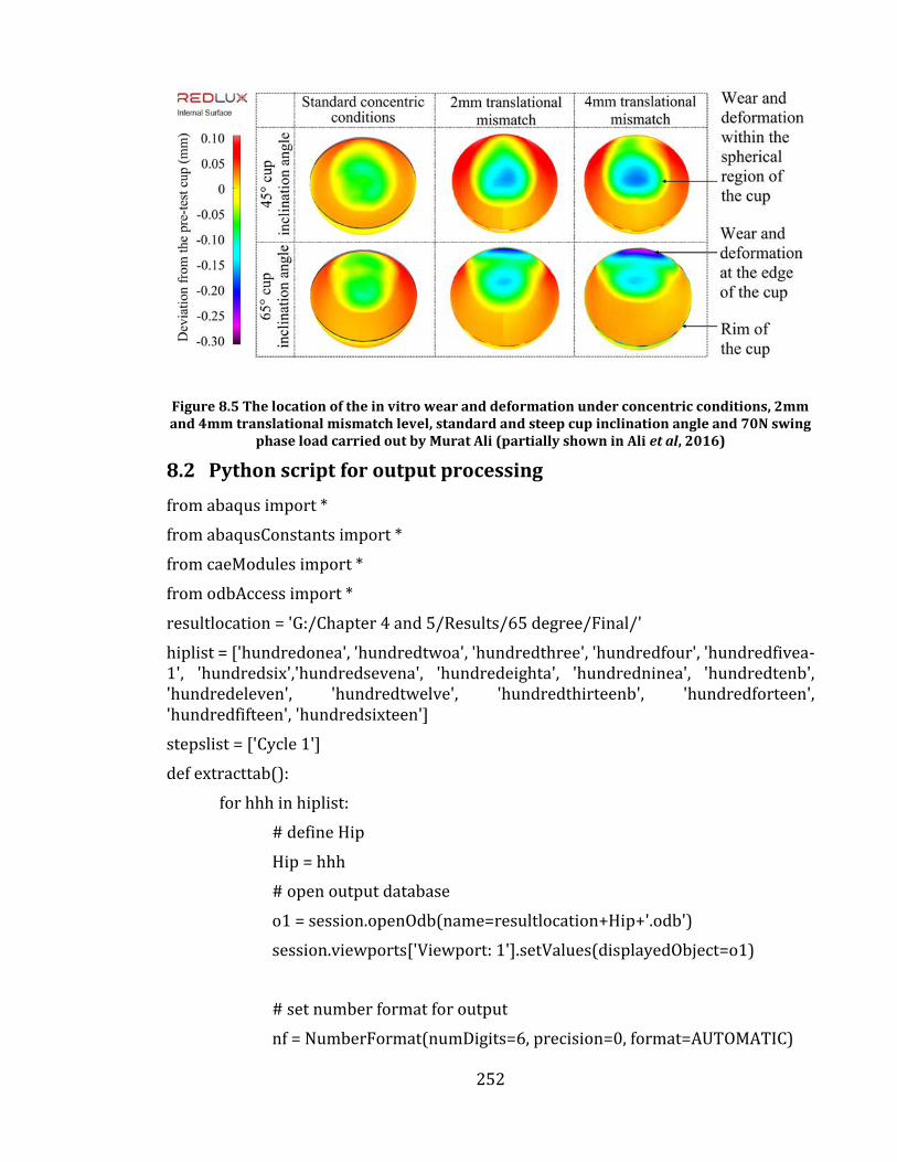
252

Figure 8.5 The location of the in vitro wear and deformation under concentric conditions, 2mm and 4mm translational mismatch level, standard and steep cup inclination angle and 70N swing

phase load carried out by Murat Ali (partially shown in Ali et al, 2016)

8.2 Python script for output processing

from abaqus import *

from abaqusConstants import *

from caeModules import *

from odbAccess import *

resultlocation = 'G:/Chapter 4 and 5/Results/65 degree/Final/'

hiplist = ['hundredonea', 'hundredtwoa', 'hundredthree', 'hundredfour', 'hundredfivea-1', 'hundredsix','hundredsevena', 'hundredeighta', 'hundredninea', 'hundredtenb', 'hundredeleven', 'hundredtwelve', 'hundredthirteenb', 'hundredforteen', 'hundredfifteen', 'hundredsixteen']

stepslist = ['Cycle 1']

def extracttab():

for hhh in hiplist:

# define Hip

Hip = hhh

# open output database

o1 = session.openOdb(name=resultlocation+Hip+'.odb')

session.viewports['Viewport: 1'].setValues(displayedObject=o1)

# set number format for output

nf = NumberFormat(numDigits=6, precision=0, format=AUTOMATIC)

253

# change viewer to poly

leaf = dgo.LeafFromPartInstance(partInstanceName=('POLY', ))

session.viewports['Viewport: 1'].odbDisplay.displayGroup.replace(leaf=leaf)

for sss in stepslist:

# get end (index is always -1) frame number for step

# try except continue means move on if no endframe exists (i.e. that step aborted)

try:

endframe=o1.steps[sss].frames[-1]

except:

continue

### CPRESS

session.fieldReportOptions.setValues(sort=DESCENDING)

session.writeFieldReport(fileName='CC'+Hip+sss+'.rpt', append=OFF,

sortItem='CPRESS', odb=o1, step=0, frame=endframe,

outputPosition=NODAL, variable=(('CPRESS', ELEMENT_NODAL), ))

### LE


session.writeFieldReport(fileName='LE'+Hip+sss+'.rpt', append=OFF,

sortItem='LE.Max. Principal', odb=o1, step=0, frame=endframe,

outputPosition=NODAL, variable=(('LE', INTEGRATION_POINT), ))

### PE


session.writeFieldReport(fileName='PE'+Hip+sss+'.rpt', append=OFF,

254

sortItem='PE.Max. Principal', odb=o1, step=0, frame=endframe,

outputPosition=NODAL, variable=(('PE', INTEGRATION_POINT), ))

### S


session.writeFieldReport(fileName='S'+Hip+sss+'.rpt', append=OFF,

sortItem='S.Mises', odb=o1, step=0, frame=endframe,

outputPosition=NODAL, variable=(('S', INTEGRATION_POINT), ))

# now extract desired lines from rpt files

# and record to text files

for hhh in hiplist:

for sss in stepslist:

reqline = 20

reqlineL = 23

# end of step

fileName='CC'+hhh+sss+'.rpt'

# get line 20

try:

with open(fileName) as f1:

i = 0

for line in f1:

if i == reqline-1:

break

i += 1

# record to file

with open("CResultop.txt", mode='a') as file:

file.write(line)

# if no data for step, record that it aborted

except:

with open("CResultop.txt", mode='a') as file:

255

file.write('Aborts \n')

# end of step

fileName='LE'+hhh+sss+'.rpt'

# get line 23

try:


i = 0

for line in f1:

if i == reqlineL-1:

break

i += 1

# record to file

with open("LEResultop.txt", mode='a') as file:

file.write(line)


except:

with open("LEResultop.txt", mode='a') as file:


# end of step

fileName='PE'+hhh+sss+'.rpt'

# get line 23

try:


i = 0

for line in f1:

if i == reqlineL-1:

break

i += 1

# record to file

with open("PEResultop.txt", mode='a') as file:

file.write(line)


256

except:

with open("PEResultop.txt", mode='a') as file:


#end of step

fileName='S'+hhh+sss+'.rpt'

# get line 23

try:


i = 0

for line in f1:

if i == reqlineL-1:

break

i += 1

# record to file

with open("SResultop.txt", mode='a') as file:

file.write(line)


except:

with open("SResultop.txt", mode='a') as file:


f1.close()

file.close()

def getstrains():

stepofint = 'Cycle 1’

# do this for steps of interest

# define list of maxU nodes found using previous function...

maxulist = [25, 474, 24, 23,473]

for Hip, MaxUnode in zip(hiplist,maxulist):

# opens odb

odb=openOdb(path='G:/Chapter 4 and 5/Results/65 degree/Final/'+Hip+'.odb')

# permanantly adds a node set

257

#odb.rootAssembly.NodeSetFromNodeLabels(name='Nodes1', nodeLabels=(('POLY',(MaxUnode, )),))

# get nodal displacements at end of named step

displacement = odb.steps[stepofint].frames[-1].fieldOutputs['CPRESS']

# get for the specific set of nodes

interestingnodes = odb.rootAssembly.nodeSets['Nodes1']

Displacement = displacement.getSubset(region=interestingnodes)

dispValues = Displacement.values

# define oc to reduce code length

oc = odb.rootAssembly.instances['POLY'].nodes

outputFile=open(Hip+'output.m','w')

outputFile.write('Nodes = [')

for u in dispValues:

outputFile.write('%d,' % (u.nodeLabel))

outputFile.write(']; \n')

outputFile.write('basex = [')


outputFile.write('%F,' % (oc[u.nodeLabel-1].coordinates[0]))


outputFile.write('basey = [')




outputFile.write('basez = [')




outputFile.close()

#outputFile.close()

# call functions

#extracttab()

#getstrains()