MODELLING OF LOADS IN POWER

FLOW ANALYSIS

SIBASISH KANUNGO (109EE0274)

Department of Electrical Engineering National Institute of Technology Rourkela

1

MODELLING OF LOADS IN POWER

FLOW ANALYSIS

A Thesis submitted in partial fulfillment of the requirements for the degree of

Bachelor of Technology in “Electrical Engineering”

By

SIBASISH KANUNGO (109EE0274)

Under guidance of

Prof. P.C PANDA

Department of Electrical Engineering National Institute of Technology

Rourkela-769008 (ODISHA) May-2013

2

DEPARTMENT OF ELECTRICAL ENGINEERING NATIONAL INSTITUTE OF TECHNOLOGY,ROURKELA

ODISHA, INDIA-769008

CERTIFICATE

This is to certify that the thesis entitled “Modelling of loads in Power Flow Analysis”,

submitted by Sibasish Kanungo (109EE0274) in partial fulfilment of the requirements for

the award of Bachelor of Technology in Electrical Engineering during session 2010-2011

at National Institute of Technology, Rourkela. A bonafide record of research work carried out

by them under my supervision and guidance.

The candidates have fulfilled all the prescribed requirements.

The Thesis which is based on candidates’ own work, have not submitted elsewhere for a

degree/diploma.

In my opinion, the thesis is of standard required for the award of a bachelor of technology

degree in Electrical Engineering.

Place: Rourkela Dept. of Electrical Engineering Prof. P.C Panda National institute of Technology Professor Rourkela-769008

3

ACKNOWLEDGEMENT:

I would remain forever obliged to The Department of Electrical Engineering, National

Institute of Technology, Rourkela for giving me the scope to carry out this project, which is

an indispensable fragment of my B. Tech curriculum. I would like to express my cordial

gratitude to my project guide, Prof. Dr. P. C. Panda, Department of Electrical Engg. ,

N.I.T Rourkela for his sincere efforts to make this project a successful one. It was his

guidance and incessant motivation during the course of uncertainties and doubts that has

helped me immensely to go ahead with this project. I would like to express my heartfelt

thankfulness Prof. A.K Panda, Head of the Department, Electrical Engineering for his

guidance and support. I am also grateful to the faculties of Electrical Engineering Department

for offering their helpful hands during the course of our project. Lastly I want to acknowledge

the contributions of my parents, family members and my friends for their constant and never

ending motivation.

a

Abstract:

The present predicament of electrical power system engineering mainly includes the

problems like blackout, power scarcity, ineptness of meeting the necessary demand of

power, load shedding etc. As a result new power plants are designed or old ones are

extended and upgraded. Load flow analysis plays a vital role in both the above mentioned

cases.

The power flow analysis provides the nodal voltages and phase angles and hence the power

injected at all the buses and power flows through interconnecting power channels. The

optimal power flow is used to optimize the load flow solutions of large scale power system.

This is done by minimizing the selected objective functions while maintaining an acceptable

limit in terms of generator capabilities and the output of the corresponding devices.

Recent decades have seen a significant development in the fields of power generation

transmission and distribution systems. Although these developments have played an

important role in today’s scenario, there still exists a field where the scope of developments

still persists.

Generally loads are taken as constant sink for both reactive and active power; Where as in

reality, the load power consumption depends magnitude of voltage and frequency deviations.

Optimal Power Flow studies incorporating load modelling is a major tool for minimizing

generation and transmission losses, generation costs and maximizing the system efficiency.

This thesis focuses on incorporation of load model in OPF analysis and comparing the results

obtained with those obtained from OPF studies without incorporating load models.

i

CONTENTS

Abstract i

Contents ii

List of Figures v

List of Tables vi

Abbreviations and Acronyms vii

CHAPTER 1

INTRODUCTION

1.1 Motivation 2

1.2 Brief Review of Power system 2

1.2.1 Classification Of Buses 3

1.3 Network Equations 3

1.4 Project Objective 4

CHAPTER 2

LOAD FLOW

2.1 Purpose Of Load Flow Analysis 6

2.2 Load Flow Solution Methods 6

2.2.1 Gauss-Siedel Technique 6

2.2.2 Newton-Raphson Technique 7

2.2.3 Fast Decoupled Method 7

2.3 System Constraints 8

2.3.1 Equality Constraints 8

2.3.2 Inequality Constraints 9

ii

2.3.2.1 Generator Constraint 9

2.3.2.2 Voltage Constraints 9

2.3.2.3 Running Spare Capacity Constraints 10

2.3.2.4 Transformer Tap Setting Constraints 10

2.3.2.5 Transmission Line Constraints 10

2.4 Optimal Power Flow 10

CHAPTER-3

MODELLING OF LOAD

3.1 Importance Of Load Modelling 13

3.2 Advantage Of Load Modelling In Power Flow Studies 13

3.3 Classification Of Load Models 13

3.4 Different Categories Of Static And Dynamics Of Load Modelling 16

3.5 Incorporation Of Static Load Models 17

CHAPTER-4

SIMULATION RESULTS AND ANALYSIS

4.1 Problem Statement 20

4.2 Analysis Of Results 27

4.2.1 Voltage Magnitude 27

4.2.2 Swing Bus Active Power 27

4.2.3 Generator Reactive Power 27

4.2.4 Load Active Power 27

4.2.5 Load Reactive Power 28

4.3 Overall Comparison 28

iii

CHAPTER-5

CONCLUSION AND FUTURE WORK

5.1 Conclusion 30

5.2 Future Work 30

References 31

iv

LIST OF FIGURES

Fig. No Name of the Figure Page. No.

4.1 A Standard IEEE 14 Bus bar System 20

4.2 Simulink Model for IEEE 14 bus system with voltage independent loads 21

4.3 Simulink model for IEEE 14 bus system incorporating voltage dependent

Loads 24

v

LIST OF TABLES

Table. No. Name of the Table Page. No.

4.1 Line Data of IEEE 14 bus bar system 22

4.2 Generator Data for IEEE 14 Bus bar System 22

4.3 Transformer Data for IEEE 14 Bus bar System 23

4.4 Synchronous Compensator Data for IEEE 14 Bus bar System 23

4.5 Voltage Independent Load Data for IEEE 14 Bus bar System 23

4.6 Load Flow Data for IEEE 14-bus system with voltage independent

Load 25

4.7 Total Demand, Losses and Generation cost for voltage independent

load 25

4.8 Power Flow Data for IEEE 14-bus system without voltage independent

load 26

4.9 Total Demand, Losses and Generation cost for voltage dependent load 26

vi

ABBREVIATIONS AND ACRONYMS

OPF - Optimal Power Flow

PSAT - Power System Analysis Toolbox

MATLAB - MATrixLABoratory

P.U. - Per Unit

N-R Technique - Newton-raphson Technique

G-S Technique - Gauss-Siedel Technique

IEEE - Institute of Electrical and Electronics Engineers

vii

1

CHAPTER1

INTRODUCTION

2

1.1 MOTIVATION

Power flow analysis is the analysis of a network under steady state condition subjected to

some inequality constraints under which the system operates. Load flow solution tells about

the line flows of reactive and active power and voltage magnitude and phase difference at

different bus bars. It is essential for design of a new power system or for planning for the

expansion of the existing one for increased load demand.

Electrical loads of a system comprises of various industrial, residential and municipal loads.

In conventional load flow studies, it is assumed that the active and reactive power demands

have specified constant values, independent of the voltage magnitudes . But in reality, the

active and reactive power of loads of a distribution system are dependent on system voltage

magnitude and frequency variations. This effects, if taken into consideration would cause a

major change in the results of load flow and OPF studies. Frequency deviation is not

considered significant in case of static analysis like, load flow studies. The effects of

voltage deviations are primarily taken into account t o get fast and accurate results and

increased system stability and security. The differences in fuel cost are more significant when

voltage dependent load models are incorporated in Optimal Power Flow (OPF) studies. The

active and reactive power demands, the stability, the losses and the voltage profile are also

affected.

1.2 BRIEF REVIEW OF POWER SYSTEM

In a power system each bus is associated with four quantities –Active and Reactive powers,

bus Voltage magnitude, and its Phase angle. In a load flow solution two out of these four

quantities are mentioned and rest are to be determined.

3

1.2.1 Classification Of Buses: The buses in the power systems are mainly classified into the

following categories:

Load Bus: At this bus the active and reactive power are specified. It is desired to

find out the magnitude of voltage and phase angle. It is not required to specify the

voltage at a load bus as the voltage can vary within a permissible limit.

Generator Bus: This is also known as voltage controlled bus. Here the net active

power and the voltage magnitude are known.

Slack Bus: Here the specified quantities are voltage magnitude and phase angle.

Slack bus is generally a generator bus which is made to take additional active and

reactive power to supply the losses caused in the network. There is one and only one

bus of this kind in a given power system. This bus is also known as Swing bus or

reference bus.

.

1.3 NETWORK EQUATIONS:

Pi(Active Power) = |Vi| k ||Yik| cos(θik+ Øk- Øi) (1.1)

Qi(Reactive Power) = |Vi| k ||Yik| sin(θik+ Øk- Øi), i=1,2, (1.2)

Where

Pi = Net active power injected at node i.

Qi = Net reactive power injected at node i.

Vi = Voltage magnitude at node i.

θik = angle associated with Yij

Øi = angle associated with V.

4

1.4 PROJECT OBJECTIVE:

The basic objective of this project is development of a voltage dependent load model in

which active and reactive powers vary exponentially with voltage and implementation of this

model in Optimal Power Flow and comparison of the results of the above with those obtained

from OPF studies without incorporation of load models to ensure minimum losses and

generation costs

5

CHAPTER 2

LOAD FLOW

6

2.1 PURPOSE OF LOAD FLOW ANALYSIS

The purpose of Load Flow analysis are as follows :

• To determine the magnitude of voltage and phase angles at all nodes of the feeder.

• To determine the line flow in each line section specified in Kilo Watt (KW) and KVAr,

amperes and degrees or amperes and power factor.

• To determine the power loss.

• To determine the total input to the feeder Kilo Watt (KW) and KVAr.

• To determine the active and reactive power of load based on the defined model for the load.

2.2 LOAD FLOW SOLUTION METHODS :

Following three methods are mostly used for the solution of a Load Flow Problem.

• Gauss-Seidel Technique.

• Newton-Raphson Technique.

• Fast-Decoupled Technique.

2.2.1 Gauss-Seidel Technique:[10]

This method of solution was named after the German mathematicians Carl Friedrich

Gauss and was upgraded b y Philipp Ludwig von Seidel. This method is defined

for matrices with non- zero diagonal elements, but converges only if the matrix is either

symmetric and positive definite or diagonally dominant. The Gauss-Seidel(GS)

technique is an iterative technique to solve a set of non-linear algebraic equations.

Ini t i a l l y a solution vector is assumed. The revised value of this particular variable

is obtained by evaluating an equation by substituting in it the present values of other

variables. The same procedure is followed for all other variables completing one

full iteration. This process is then repeated till the solution vector converges within a

7

permissible error limits. The degree of convergence is quite sensitive to the initial

values that are assumed.

Vi =

[((Pi-jQi)/Vi

*) –

] (2.3)

2.2.2 Newton - Raphson Technique:

Newton-Raphson technique is an iterative process in which a set of non-linear

simultaneous equations is approximated into a set of linear simultaneous equations using

Taylor’s series expansion. In an N-bus bar power system there are n equations for

active power flow Pi and n-equations for reactive power flow Qi. The number of

unknowns are 2(n-1) because the voltage at the slack or swing bus is known and is kept

constant both in magnitude and phase.

=

(2.4)

∆Pi = Pi(Specified) - Pi

∆Qi = Qi(Specified) - Qi

is the mismatch vector.

is the correction matrix.

2.2.3 Fast Decoupled Method:

The Fast decoupled method is a derivative of Newton-Raphson technique which is

designed in polar coordinates with some approximations that results in a fast algorithm

for load flow solution. Though this method requires more iterations than the Newton-

8

Raphson method, but still consumes significantly less time per iteration and a solution to

load flow problem is obtained quickly. This method finds numerous applications in

contingency analysis where numerous outages are to be simulated or a load flow solution

is required for on-line control.

2.3 SYSTEM CONSTRAINTS:[1]

There are two types of constraints.

• Equality constraints.

• Inequality constraints.

Inequality constraints are further classified into two categories, i.e.

1) Hard Type - The hard type constraints have constant and definite values for ex-

the tapping range of an on load tap changing transformer. These constraints are

very rigid in their values and don’t entertain changes in them.

2) Soft Type - The soft type constraints are not very rigid to changes and offer some

flexibility in changing their values, for ex - phase angles and nodal voltages.

2.3.1 Equality Constraints:

The basic equality constraints are:

Pp = ep(eqGpq + fqBpq) + fp(fqGpq - epBpq)} (2.5)

Qp = fp(eqGpq + fqBpq) - ep(fqGpq - epBpq)} (2.6)

Where Vp = ep + jfp (real and imaginary components of voltage at the pth node)

And Ypq = Gpq - jBpq (the nodal conductance and susceptance)

9

2.3.2 Inequality Constraints:[1]

The following are the primary categories of inequality constraints:

Generator constraints.

Voltage constraints

Running spare capacity constraints.

Transformer tap settings.

Transmission line constraints.

2.3.2.1 Generator Constraints :

Ppmin ≤ Pp ≤ Ppmax and Qpmin ≤ Qp ≤ Qpmax

Thermal consideration limits the maximum active power generation where as flame

instability of a boiler limits the minimum active power generation. Similarly the maximum

and minimum reactive power generation is limited by overheating of the rotor and the

stability limit of the machine respectively

2.3.2.2 Voltage Constraints :

| Vpmin | ≤ |Vp| ≤ |Vpmax| and δpmin ≤ δp ≤ δpmax

The variation in voltage magnitude should be within a prescribed limit for satisfactory

operation of the equipments connected to the system otherwise additional use of voltage

regulators will make the system cost ineffective.

10

2.3.2.3 Running Spare Capacity Constraints:

These constraints are needed during the incident of ● forced outages of one or more

alternators of the system and ● the unexpected load in the system.

The total generation should be in a such way that in addition to meet the load demand and

losses a ,minimum spare should be available.

2.3.2.4 Transformer Tap Setting Constraints :

The minimum tap setting in an auto transformer should be zero and the maximum

should be one i.e. 0 ≤ t ≤ 1.

Similarly if tappings are provided on the secondary side of a two winding transformer then,

0 ≤ t ≤ n, Where n is the ratio of transformation.

2.3.2.5 Transmission Line Constraints :

Thermal capability of the circuit limits the flow of active and reactive power through the

transmission line and is expressed as Cp ≤ Cpmax, where Cpmax defines the maximum loading

capacity of the pth line.

2.4 OPTIMAL POWER FLOW:

Practically the generating stations are never equidistant from the load centres and their fuel

costs are never the same. Also, Generally the generation capacity surpasses the total demand

and losses. This investigates the need for scheduling generation. In an interconnected power

system, the primary objective is to keep a track of the real and reactive power scheduling of

each power plant in order to reduce the operating cost. Thus the generator’s active and

reactive power have flexibility to vary within defined limits to satisfy the load demand with

the lowest possible operating cost. This is defined as Optimal Power Flow (OPF) problem.

The considerations like economy of operation, fossil fuel emissions, security of system and

11

optimal release of water at hydro generation plants are involved in the optimal system

operation. The primary objective of the economic load dispatch problem is to minimize the

total generating cost at various generating stations while meeting the load demands and the

loses in transmission links.

Based on the problem requirement an OPF model may inculcate various control variables and

system constraints. Among the control variables, an OPF can include the following:[9]

Real and reactive power generation.

Switched capacitor settings.

Load MVA and MVAr (Load shedding)

OLTC transformers tap changing.

12

CHAPTER 3

MODELLING OF LOAD

13

3.1 IMPORTANCE OF LOAD MODELLING : The choices regarding system reinforcements and system performance is mostly based on the

results of power flow and stability simulation studies. For performing analysis of power

system, models must be integrated to include all relevant system components, such as

generating stations, sub stations, transmission and distribution peripherals and load devices.

Much attention has been given to modelling of generation and transmission or distribution

devices. But the modelling of loads have received much less attention and remains to be an

unexplored frontier and carries much scope for future development. Recent studies have

revealed that representation and modelling of load can have a great impact on analysis

results. Efforts in the directions of improving load-models have been given prime importance.

3.2 ADVANTAGES OF LOAD MODELLING IN POWER FLOW STUDIES:[10]

The variation of power demand with voltage enables better control capacity.

Actual calculation of active and reactive power demand at respective buses.

Control of over and under voltage at load buses.

Minimization of losses.

Improvement in voltage profile.

Reduction of Incremental Fuel Cost.

3.3 CLASSIFICATION OF LOAD MODELS :

Load models are broadly classified into two groups:

Static Load Model : [3]

This model expresses the reactive and active power, at a particular instant of time, as a

function of the magnitude of bus bar voltage and frequency. Both static and dynamic load

14

components use static load models. The static load is model is given as an exponential

function of voltage, V

Pd = P0 (V/V0)α

(3.7)

Qd = Q0 (V/V0)β (3.8)

Where,

Pd = Active power demand of load.

Qd = Reactive power demand of load.

P0 = Consumption of active power at rated voltage, V0.

Q0 = Consumption of reactive power at rated voltage, V0.

α = Active power expoment.

β = Reactive power expoment.

V = Supply voltage.

V0 = Rated voltage

Dynamic Load Models :

In Dynamic load model the active and reactive power at a particular instant of time is

represented as a function of the magnitude of voltage and frequency. Dynamic load models

are often used in studies regarding voltage stability, inter-area oscillations and long term

stability. Such models are mostly represented using differential equations.

Input-Output Form :

TpṖd + Pd = Ps(v) + Kp(v)V∙

(3.9)

TpQ∙d + Qd = Qs(v) + Kq(v)V

∙ (3.10)

Kp(v) = TpPt(v) (3.11)

Kq(v) = TqQt(v)’ (3.12)

Ps = P0 {

}αs

(3.13)

Qs = Q0 {

}βs

(3.14)

15

Pt = P0 {

}αt

(3.15)

Qt = Q0 {

}βt

(3.16)

State Form :

TpẊp = Ps(v) – Pd (3.17)

TqẊq = Qs(v) – Qd (3.18)

Where,

Tp = Recovery time constant of active load.

Tq = Recovery time constant of reactive load.

Pd = Model of active power consumption.

Qd = Model of reactive power consumption.

Ps(v) = Steady-state part of active power consumption.

Qs(v) = Steady-state part of reactive power consumption.

Pt(v) = Transient part of active power consumption.

Qt(v) = Transient part of reactive power consumption.

αs = Steady-state active load-voltage dependence.

βs = Steady-state reactive load-voltage dependence.

αt = Transient active load-voltage dependence.

βt = Transient reactive load-voltage dependence.

P0 = Consumption of active power at rated voltage, Vo.

Q0 = Consumption of reactive power at rated voltage, Vo.

V= Supply voltage.

V0 = Supply voltage during pre-fault conditions .

16

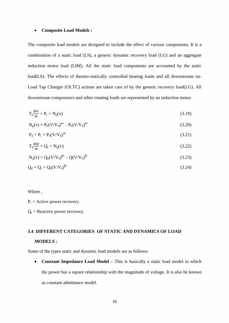
Composite Load Models :

The composite load models are designed to include the effect of various components. It is a

combination of a static load (LS), a generic dynamic recovery load (LG) and an aggregate

induction motor load (LIM). All the static load components are accounted by the static

load(LS). The effects of thermo-statically controlled heating loads and all downstream on-

Load Tap Changer (OLTC) actions are taken care of by the generic recovery load(LG). All

downstream compressors and other rotating loads are represented by an induction motor.

Tp

+ Pr = Np(v) (3.19)

Np(v) = P0(V/V0)αs

– P0(V/V0)αt

(3.20)

Pd = Pr + P0(V/V0)αt

(3.21)

Tq

+ Qr = Nq(v) (3.22)

Nq(v) = Q0(V/V0)βs

– Q(V/V0)βt

(3.23)

Qd = Qr + Q0(V/V0)βt

(3.24)

Where ,

Pr = Active power recovery.

Qr = Reactive power recovery.

3.4 DIFFERENT CATEGORIES OF STATIC AND DYNAMICS OF LOAD

MODELS :

Some of the types static and dynamic load models are as follows:

Constant Impedance Load Model – This is basically a static load model in which

the power has a square relationship with the magnitude of voltage. It is also be known

as constant admittance model.

17

Constant Current Load Model – It is a static load model in which the power has a

linearly relationship with voltage magnitude.

Constant Power Load Model – This is a static load model where power is

independent of variation in voltage magnitude. It is also known constant MVA model.

Polynomial Load Model – It is a static load model where power has a polynomial

relationship with voltage magnitude as shown below.

P = P0[a0(V/V0)2 + a1(V/V0) + a2] (3.25)

Q = Q0[b0(V/V0)2 + b1(V/V0) + b2] (3.26)

Where, a0 + a1 + a2 = 1 and b0 + b1 + b2 =1

This model is also called “ZIP” model as it cumulates all the above models into a

single expression.

Exponential Load Model – It is a static load model which represents power as an

exponential function of voltage magnitude.

3.5 INCORPORATION OF STATIC LOAD MODEL :

Incorporation of the load model in load flow solution is best achieved by writing Newton-Raphson

method in its polar co-ordinates form –

Pd = P0 (V/V0)α

and Qd = Q0 (V/V0)β

By differentiating the above equation w.r.t V, we get

= P0.α.(

(α-1)

.

+

(

)α (3.27)

= Q0.β.(

(β-1)

.

+

(

)β (3.28)

18

We know –

= 2|Vi||Yij|cos( ij) +

Vk||Yik|cos(θik + θk + j) (3.29)

= 2|Vi||Yij|cos( ij) +

Vk||Yik|sin(θik + θk + j) (3.30)

Combining both the equations we get –

= P0.α.(

(α-1)

.

+ (

)α[2|Vi||Yij|cos( ij) +

Vk||Yik|cos(θik + θk + j)] (3.31)

= Q0.β.(

(β-1)

.

+ (

)β [2|Vi||Yij|cos( ij) +

Vk||Yik|sin(θik + θk + j)] (3.32)

Further calculations are completely based on the above two equations. The jacobian matrix is

evaluated using the above equations and results of OPF are obtained.

19

CHAPTER 4

SIMULATION RESULTS

AND ALANYSIS

20

4.1 PROBLEM STATEMENT A standard IEEE 14 bus system was considered for analysis both with conventional load flow

method and load flow incorporating voltage dependent load models[10]. The simulations

were made using Matlab Power system toolbox known as PSAT (Power System Analysis

Toolbox)[8]. The results of the simulations were plotted and analyzed.

Fig 4.1 A Standard IEEE 14 Bus bar System

21

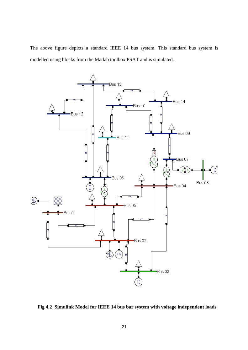
The above figure depicts a standard IEEE 14 bus system. This standard bus system is

modelled using blocks from the Matlab toolbox PSAT and is simulated.

Fig 4.2 Simulink Model for IEEE 14 bus bar system with voltage independent loads

22

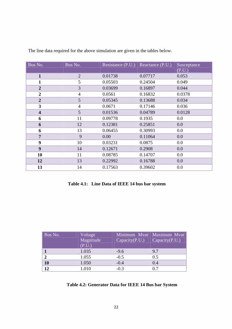
The line data required for the above simulation are given in the tables below.

Table 4.1: Line Data of IEEE 14 bus bar system

Bus No. Voltage

Magnitude

(P.U.)

Minimum Mvar

Capacity(P.U.)

Maximum Mvar

Capacity(P.U.)

1 1.035 -9.6 9.7

2 1.055 -0.5 0.5

10 1.050 -0.4 0.4

12 1.010 -0.3 0.7

Table 4.2: Generator Data for IEEE 14 Bus bar System

Bus No. Bus No. Resistance (P.U.) Reactance (P.U.) Susceptance

(P.U.)

1 2 0.01738 0.07717 0.053

1 5 0.05503 0.24504 0.049

2 3 0.03699 0.16897 0.044

2 4 0.0561 0.16832 0.0378

2 5 0.05345 0.13688 0.034

3 4 0.0671 0.17146 0.036

4 5 0.01536 0.04789 0.0128

6 11 0.09778 0.1935 0.0

6 12 0.12381 0.25851 0.0

6 13 0.06455 0.30993 0.0

7 9 0.00 0.11064 0.0

9 10 0.03231 0.0875 0.0

9 14 0.12671 0.2908 0.0

10 11 0.08785 0.14707 0.0

12 13 0.22992 0.16788 0.0

13 14 0.17563 0.39602 0.0

23

Transformer Designation Tap Settings(Per Unit)

5-6 0.942

4-9 0.956

4-7 0.986

7-8 0.954

Table 4.3: Transformer Data for IEEE 14 Bus bar System

Bus No. Voltage

Magnitude

(P.U.)

Minimum Mvar

Capacity(P.U.)

Maximum Mvar

Capacity(P.U.)

3 1.03 0.0 0.4

8 1.06 -0.05 0.25

6 1.08 -0.04 0.25

12 1.025 -0.6 0.6

Table 4.4: Synchronous Compensator Data for IEEE 14 Bus bar System

Bus No. Load Active Power (P.U.) Load Reactive Power (P.U.)

2 0.1044 0.0024

3 1.3158 0.286

4 0.6752 0.046

5 0.1044 0.0024

6 0.1688 0.106

9 0.465 0.2334

10 0.123 0.0852

11 0.045 0.02342

12 0.0654 0.0278

13 0.156 0.0856

14 0.2146 0.08

Table 4.5: Voltage Independent Load Data for IEEE 14 Bus bar System

24

To proceed further the voltage independent loads are replaced by voltage dependent loads

and remodelled using the blocks from PSAT as shown below.

Fig 4.3 Simulink model for IEEE 14 bus system incorporating voltage dependent loads

25

Table 4.6: Load Flow Data for IEEE 14-bus system with voltage independent load

Total Generation(MW) 107.9276

Total Demand(MW) 90.99

Total Losses(MW) 16.9376

Generation Cost(Rs/hr) 165.2545

Table 4.7: Total Demand, Losses and Generation cost for voltage independent load

Bus No. Voltage

Magnitude

Angle(Radians) Laod

Generation

MW MVar MW MVar

1 1.2 0 23.25 14.4567 16.871 17.876

2 1.167 -0.056 8.780 35.22 91.0566 49.345

3 1.126 -0.22 12.01 13.56 0.00 40.86

4 1.124 -0.178 6.98 5.6 0.00 0.00

5 1.130 -0.154 7.56 2.24 0.00 0.00

6 1.173 -0.267 5.75 13.5 0.00 24.56

7 1.147 -0.274 0.00 0.00 0.00 0.00

8 1.153 -0.247 0.00 2.6 0.00 24

9 1.1566 -0.289 4.43 23.54 0.00 0.00

10 1.125 -0.270 4.67 8.67 0.00 0.00

11 1.144 -0.294 3.78 3.56 0.00 0.00

12 1.151 -0.286 7.54 1.27 0.00 0.00

13 1.152 -0.310 2.56 7.67 0.00 0.00

14 1.1103 -0.304 3.68 8.01 0.00 0.00

26

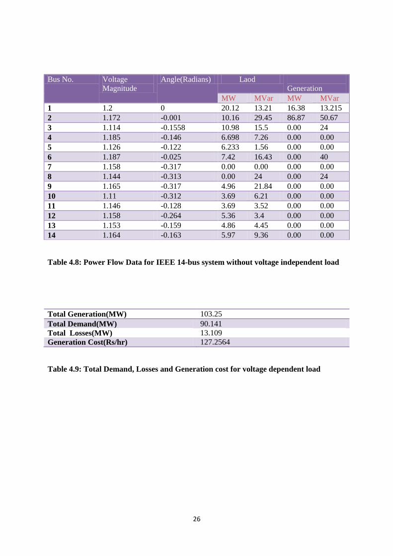
Table 4.8: Power Flow Data for IEEE 14-bus system without voltage independent load

Total Generation(MW) 103.25

Total Demand(MW) 90.141

Total Losses(MW) 13.109

Generation Cost(Rs/hr) 127.2564

Table 4.9: Total Demand, Losses and Generation cost for voltage dependent load

Bus No. Voltage

Magnitude

Angle(Radians) Laod

Generation

MW MVar MW MVar

1 1.2 0 20.12 13.21 16.38 13.215

2 1.172 -0.001 10.16 29.45 86.87 50.67

3 1.114 -0.1558 10.98 15.5 0.00 24

4 1.185 -0.146 6.698 7.26 0.00 0.00

5 1.126 -0.122 6.233 1.56 0.00 0.00

6 1.187 -0.025 7.42 16.43 0.00 40

7 1.158 -0.317 0.00 0.00 0.00 0.00

8 1.144 -0.313 0.00 24 0.00 24

9 1.165 -0.317 4.96 21.84 0.00 0.00

10 1.11 -0.312 3.69 6.21 0.00 0.00

11 1.146 -0.128 3.69 3.52 0.00 0.00

12 1.158 -0.264 5.36 3.4 0.00 0.00

13 1.153 -0.159 4.86 4.45 0.00 0.00

14 1.164 -0.163 5.97 9.36 0.00 0.00

27

4.2 ANALYSIS OF RESULTS

4.2.1 Voltage Magnitude

The data obtained from table 6 and 8 shows the voltage magnitudes at different buses. It can

be observed that, in case of loads that are voltage independent, the magnitude of voltages are

less in value in comparison to that of voltage dependent loads. In the former case, the

generation of active power is more pronounced when magnitude of voltages are greater than

1 p.u. Incorporation of voltage dependent loads confirms a flat voltage profile, i.e. the load

flow increases magnitudes of voltages below 1 p.u and decreases those above 1 p.u.

4.2.2 Swing bus Active Power

In both the type of loads the swing bus active power difference is 2.5 %. This is a quite high

value and accounts for net decrease in power generation and hence the reduced cost of

operation. The active power difference of swing bus is dependent both on voltage and phase

angle difference and practically is very tough to predict from conventional load flow analysis

without the incorporation of voltage dependent loads.

4.2.3 Generator Reactive Power

The difference in reactive power lies in the range of 4 % to 16 %. This range is even greater

the swing bus active power difference. A generator bus which had reached the reactive-power

limits in conventional load-flow analysis was well within the limits when the load was

modelled to vary with voltage. The generator reactive power difference is also dependent on

phase angle differences and voltage magnitudes.

4.2.4 Load Active Power

Table 6 and 8 gives information about the Load active powers at different buses. The active

power consumption at different buses in case of voltage dependent and independent loads are

not equal. In case of the voltage dependent loads, the real power consumption is less as

28

compared to the voltage independent loads. Decrease in active power consumption ensures

less loss and better stability and security of the system.

4.2.5 Load Reactive Power

The reactive power at different buses don’t follow any particular pattern, i.e. at some buses

they have higher values for voltage dependent loads and at some, they have lower values. But

basically the difference ranges from 0.6 % to 4.2 %.

4.3 Overall Comparison

A cumulative study of total demand, losses, generation and generation costs are made and

plotted in Fig. 8. It is deduced from the overall comparison that, in case of load modelling

each of the above mentioned quantities have a lower value as compared to that of

conventional load flow. There is a marginal decrease in generation cost and total losses. A

basic cost analysis is given below to emphasize the importance load modelling.

Generation cost for voltage independent loads = Rs 165.2545/Hr

Generation cost for voltage dependent loads = Rs 127.2564/Hr

Difference in generation cost per hour = Rs 37.9981

Difference in generation cost per day = 37.0607*24 = Rs 911.9544

Difference in generation cost per year = 889.4568*365 = Rs 332863.356

29

CHAPTER 5

CONCLUSION AND

FUTURE WORK

30

5.1 CONCLUSION This Project introspects the effects of incorporation of load models i.e. the variation of active

and reactive power demands with magnitude of voltage at different buses in load flow

analysis. The simulation of a standard IEEE 14 bus bar system was conducted and the effects

of load modelling were also incorporated in the experiment.

The effect of load modelling could be observed with the pronounced difference in fuel cost.

The heavier the loading of the system, the lower is the fuel cost difference[3].

Implementation of load model brings a significant reduction in the generation cost for the

whole year. The calculations become more accurate and system security and stability increase

by incorporating the voltage dependent load models.

The reactive power modelling greatly affects the voltage difference, whereas the active power

modelling has a greater effect on phase angle differences. The total power generation is not

much affected by the incorporation of load models but this small difference in generation

power affects the generation cost difference and total losses because the generation cost

function depends on square of generating power. The voltage profile remains flat which adds

to the advantages of incorporation of load models. Thus it is deduced that incorporation of

load models in load flow analysis is advantageous than conventional load flow analysis as

generation costs and losses are reduced and security and stability of the system increases.

5.2 FUTURE WORK

This thesis basically models variation of active and reactive power with voltage and neglects

the effect of frequency on them. Basically for easier computation static load models are

considered here. Load modelling taking into account the effect of frequency on active and

reactive power demand and dynamics of load can bring more accuracy to the results obtained.

31

REFERENCES:

[1]. C. L. Wadhwa (2009), “Electrical Power Systems”, Chap 18, Chap 19.

[2]. Dommel, H.W. and Tinney, W. F. “Optimal Power Flow Solutions”, IEE

Transactions on power apparatus and systems, Vol Pas-87, No. 10, October 1968

[3]. Dias, L. G. And M.E.El-Hawary “Effects of active and reactive power modelling on

optimal load flows”, IEE PROCEEDINGS, Vol. 136, Pt. C, No. 5, September 1989

[4]. Dias, L. G. And M.E.El-Hawary “Incorporation of load models in load flow studies”,

IEE PROCEEDINGS, Vol. 134, Pt. C, No. 1, January 1987

[5]. Dias, L. G. And M.E.El-Hawary “OPF Incorporating load models maximizing net

revenue”, IEEE Transactions on Power Systems, Vol. 8,No. 1, February 1993

[6]. Saadat H.(2010), "Power System Analysis", Chap 6, Chap 7.

[7]. MATLAB, Version 2009, MathWorks.

[8]. Milano, Federico, “Power System Analysis Toolbox”, July 2005

[9]. M.A Pai,“Operation Of Reconstructed Power System”, Chap 2

[10].Sambit Kumar Dwivedi, “Load Modelling In Optimal Power Flow Studies”,http://

ethesis@nitrkl.ac.in

32