Journal of

Imaging

Article

Modelling of Orthogonal Craniofacial Profiles

Hang Dai 1,*, Nick Pears 1 and Christian Duncan 2

1 Department of Computer Science, University of York, Heslington, York YO10 5GH, UK;nick.pears@york.ac.uk

2 Alder Hey Children’s Hospital, Liverpool L12 2AP, UK; Christian.Duncan@alderhey.nhs.uk* Correspondence: hd816@york.ac.uk; Tel.: +44-1904-325-643

Received: 20 October 2017; Accepted: 23 November 2017; Published: 30 November 2017

Abstract: We present a fully-automatic image processing pipeline to build a set of 2D morphablemodels of three craniofacial profiles from orthogonal viewpoints, side view, front view and topview, using a set of 3D head surface images. Subjects in this dataset wear a close-fitting latex capto reveal the overall skull shape. Texture-based 3D pose normalization and facial landmarking areapplied to extract the profiles from 3D raw scans. Fully-automatic profile annotation, subdivisionand registration methods are used to establish dense correspondence among sagittal profiles.The collection of sagittal profiles in dense correspondence are scaled and aligned using GeneralisedProcrustes Analysis (GPA), before applying principal component analysis to generate a morphablemodel. Additionally, we propose a new alternative alignment called the Ellipse Centre Nasion (ECN)method. Our model is used in a case study of craniosynostosis intervention outcome evaluation, andthe evaluation reveals that the proposed model achieves state-of-the-art results. We make publiclyavailable both the morphable models and the profile dataset used to construct it.

Keywords: morphable model; shape modelling; craniofacial; craniosynostosis

1. Introduction

In the medical analysis of craniofacial shape, the visualisation of 2D profiles [1] is highlyinformative when looking for deviations from population norms. It is often useful, in terms of visualclarity and attention focus, for the clinician to examine shape outlines from canonical viewpoints;for example, pre- and post-operative canonical profiles can be overlaid. We view profile-basedmodelling and analyses as being complementary to that of a full 3D shape model. Profile visualisationsshould be backed up by quantitative analysis, such as the distance (in standard deviations) of a patient’sshape profile from the mean profile of a reference population. Therefore, we have developed a novelimage processing pipeline to generate a 2D morphable model of craniofacial profiles from a set of3D head surface images. We construct morphable 2D profile models over three orthogonal planes toprovide comprehensive models and analyses of shape outline.

A morphable model is constructed by performing some form of dimensionality reduction,typically Principal Component Analysis (PCA), on a training dataset of shape examples. This isfeasible only if each shape is first re-parametrised into a consistent form where the number of pointsand their anatomical locations are made consistent to some level of accuracy. Shapes satisfying theseproperties are said to be in dense correspondence with one another. Once built, the morphable modelprovides two functions. Firstly, it is a powerful prior on 2D profile shapes that can be leveraged in fittingalgorithms to reconstruct accurate and complete 2D representations of profiles. Secondly, the proposedmodel provides a mechanism to encode any 2D profile in a low dimensional feature space; a compactrepresentation that makes tractable many 2D profile analysis problems in the medical domain.

Contributions: We propose a new pipeline to build a 2D morphable model of the craniofacialsagittal profile and augment it with profile models from frontal and top down views. We also integrate

J. Imaging 2017, 3, 55; doi:10.3390/jimaging3040055 www.mdpi.com/journal/jimaging

J. Imaging 2017, 3, 55 2 of 15

all three profiles into a single model, thus capturing any correlations within and between the threeprofile shapes more explicitly and clearly than is possible with PCA analysis on a full 3D model.A new pose normalisation scheme is presented called Ellipse Centre Nasion (ECN) normalisation.Extensive qualitative and quantitative evaluations reveal that the proposed normalisation achievesstate-of-the-art results. We use our morphable model to perform craniosynostosis intervention outcomeevaluation on a set of 25 craniosynostosis patients. For the benefit of the research community, wewill make publicly available (on email request to the first author) the three profile datasets overa 1212-subject dataset; all of our 2D morphable models will be downloadable with MATLAB GUI codeto view and manipulate the models.

Paper structure: In the following section, we discuss related literature. Section 3 discusses our newpipeline used to extract profiles and construct 2D morphable models. The next section evaluates severalvariants of the constructed models both qualitatively and quantitatively, while Section 5 compares oursingle-view models with our multi-view model. Section 6 illustrates the use of the morphable modelin intervention outcome assessment for a population of 25 craniosynostosis patients. A final sectionconcludes the work.

2. Related Work

In the late 1990s, Blanz and Vetter built a ‘3D Morphable Model’ (3DMM) from 3D facescans [2] and employed it in a 2D face recognition application [3]. Two hundred scans wereemployed (young adults, 100 males and 100 females). Dense correspondences were computedusing a gradient-based optic flow algorithm; both shape and colour-texture are used. The model isconstructed by applying PCA to shape and colour-texture (separately).

The Basel Face Model (BFM) is the most well-known and widely-used face model and wasdeveloped by Paysan et al. [4]. Again, 200 scans were used, but the method of determiningcorresponding points was improved. Instead of optic flow, a set of hand-labelled feature pointsis marked on each of the 200 training scans. The corresponding points are known on a template mesh,which is then morphed onto the training scan using underconstrained per-vertex affine transformations,which are constrained by regularisation across neighbouring points [5]. Recently, a similar morphingstrategy was used to build a facial 3DMM from a much larger dataset (almost 10,000 faces) [6], althoughthere is no cranial shape information in the model.

The Iterative Closest Points (ICP) algorithm [7,8] is the basic method to address the pointregistration problem. Several extensions of ICP for the non-rigid case were proposed [5,9–13]. Otherdeformable template methods could be used to build morphable models [14,15], such as Thin PlateSplines (TPS) [16], TPS with Robust Point Matching (TPS-RPM) [17], the non-rigid point and normalregistration algorithm of Lee et al. [18], relaxation labelling [19] or the manifold learning methodof Ma et al. [20]. The global correspondence optimization method solves simultaneously for bothdeformation parameters, as well as the correspondence positions [21]. Myronenko et al. consider thealignment of two point sets as a probability density estimation [22], and they call the method CoherentPoint Drift (CPD); this remains a highly competitive template morphing algorithm.

Template morphing methods need an automatic initialisation to bring them within theconvergence basin of the global minimum of alignment and morphing. To this end, Active AppearanceModels (AAMs) [23] and elastic graph matching [24] are the classic approaches of facial landmarkand pose estimation. Many improvements over AAM have been proposed [25,26]. Recent work hasfocused on global spatial models built on top of local part detectors, sometimes known as ConstrainedLocal Models (CLMs) [27,28]. Zhu and Ramanan [29] use a tree structured part model of the face,which both detects faces and locates facial landmarks. One of the major advantages of their approachis that it can handle extreme head pose.

Another relevant model-building technique is the Minimum Description Length method(MDL) [30], which selects the set of parameterizations that build the ‘best’ model, where ‘best’ isdefined as that which minimizes the description length of the training set.

J. Imaging 2017, 3, 55 3 of 15

3. Model Construction Pipeline

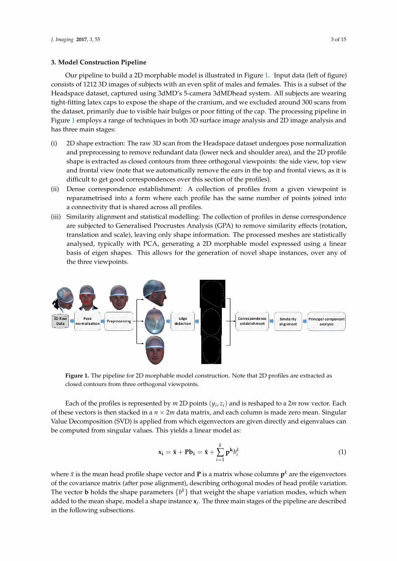
Our pipeline to build a 2D morphable model is illustrated in Figure 1. Input data (left of figure)consists of 1212 3D images of subjects with an even split of males and females. This is a subset of theHeadspace dataset, captured using 3dMD’s 5-camera 3dMDhead system. All subjects are wearingtight-fitting latex caps to expose the shape of the cranium, and we excluded around 300 scans fromthe dataset, primarily due to visible hair bulges or poor fitting of the cap. The processing pipeline inFigure 1 employs a range of techniques in both 3D surface image analysis and 2D image analysis andhas three main stages:

(i) 2D shape extraction: The raw 3D scan from the Headspace dataset undergoes pose normalizationand preprocessing to remove redundant data (lower neck and shoulder area), and the 2D profileshape is extracted as closed contours from three orthogonal viewpoints: the side view, top viewand frontal view (note that we automatically remove the ears in the top and frontal views, as it isdifficult to get good correspondences over this section of the profiles).

(ii) Dense correspondence establishment: A collection of profiles from a given viewpoint isreparametrised into a form where each profile has the same number of points joined intoa connectivity that is shared across all profiles.

(iii) Similarity alignment and statistical modelling: The collection of profiles in dense correspondenceare subjected to Generalised Procrustes Analysis (GPA) to remove similarity effects (rotation,translation and scale), leaving only shape information. The processed meshes are statisticallyanalysed, typically with PCA, generating a 2D morphable model expressed using a linearbasis of eigen shapes. This allows for the generation of novel shape instances, over any ofthe three viewpoints.

Figure 1. The pipeline for 2D morphable model construction. Note that 2D profiles are extracted asclosed contours from three orthogonal viewpoints.

Each of the profiles is represented by m 2D points (yi, zi) and is reshaped to a 2m row vector. Eachof these vectors is then stacked in a n× 2m data matrix, and each column is made zero mean. SingularValue Decomposition (SVD) is applied from which eigenvectors are given directly and eigenvalues canbe computed from singular values. This yields a linear model as:

xi = x + Pbi = x +k

∑i=1

pkbki (1)

where x is the mean head profile shape vector and P is a matrix whose columns pk are the eigenvectorsof the covariance matrix (after pose alignment), describing orthogonal modes of head profile variation.The vector b holds the shape parameters {bk} that weight the shape variation modes, which whenadded to the mean shape, model a shape instance xi. The three main stages of the pipeline are describedin the following subsections.

J. Imaging 2017, 3, 55 4 of 15

3.1. 2D Shape Extraction

2D shape extraction requires three stages, namely (i) pose normalisation, (ii) cropping and(iii) edge detection. Each of these stages is described in the following subsection.

3.1.1. Pose Normalisation

Using the colour-texture information associated with the 3D mesh, we can generate a realistic 2Dsynthetic image from any view angle. We rotate the scan over 360 degrees in pitch and yaw (10 stepsof each) to generate 100 images. Then, the Viola–Jones face detection algorithm [31] is used to find thefrontal face image among this image sequence. A score is computed that indicates how frontal thepose is. The 2D image with the highest score is chosen to undergo 2D facial landmarking. We employthe method of Constrained Local Models (CLMs) using robust discriminative response map fitting [32]to do the 2D facial image landmarking. Then, the trained system is used to estimate the three anglesfor the image with facial landmarks. Finally, 3D facial landmarks are captured by projecting the 2Dfacial landmarks to the 3D scan. As shown in Figure 2, by estimating the rigid transformation matrix Tfrom the landmarks of a 3D scan to that of a template, a small adjustment of pose normalization isimplemented by transforming the 3D scan using T−1.

Figure 2. 3D pose normalization using the texture information.

3.1.2. Cropping

3D facial landmarks can be used to crop out redundant points, such as the shoulder area and longhair. The face landmarks delineate the face size and its lower bounds on the pose normalised scan,allowing any of several cropping heuristics to be used. We calculate the face size by computing theaverage distance from facial landmarks to their centroid. Subsequently, a plane for cropping the 3Dscan is generated by moving the cropping plane downward an empirical percentage of the face size.We use a sloping cropping plane so that the chin area is included, but that still allows us to crop closeto the base of the latex skull cap at the back of the neck to remove the (typically noisy) scan region,where the subject’s hair emerges from under the cap (see Figure 1).

3.1.3. Edge Detection

We use side view, top view and frontal view from the 3D scan to reveal the 2D profile shape, andwe can generate a 2D contour within the three views by orthogonal projection. For example, in the sideview (Y-Z view), we traverse the Y direction in small steps, and at each step, we compute the minimumand maximum Z value. The points with the minimum and maximum Z value are the contour pointsin the side view.

J. Imaging 2017, 3, 55 5 of 15

3.1.4. Automatic Annotation

A machine learning method of finding approximate facial landmark localisations was describedin Section 3.1.1. The (y, z) positions of these landmarks are used to indicate the approximate locationsof landmarks on the extracted profile, by closest point projection. These can be considered as initialapproximate landmark positions, which then can be refined by a local optimisation, based on a discoperator applied to the local structure of the profile. In this method, we centre a disc (at the largestscale that we are interested in) on some point on the head profile and fit, by least squares, a quarticpolynomial to the profile points within that disc. A quartic was chosen to give the flexibility to fit tothe ‘double peaked’ area over the lips. Thus, we find quartic parameters pT to fit a set of profile points[xp, yp] such that, with n = 4:

yp = pTxp, p = [p0...pn]T , xp = [x0

p...xnp]

T (2)

To implement our disc operator, we take a dense, regularly-spaced set of n point samples withinthat disc, [xd, yd] and compute the operator value as:

α =1n

n

∑i=1

sign(yd − pTxd) (3)

We find that (−1 ≤ α ≤ 1), with values close to zero indicating locally flat regions, positive valuesindicating convexities, such as the pronasale (nose tip), and negative values indicating concavities, suchas the nasion. Effectively, this is a discrete approximation to finding the area within the facial profilethat intersects with a disc of some predefined scale. The discrete sampling gives a high frequencyquantisation noise on the signal, and so, we filter this with a 10th order low pass Butterworth filter.

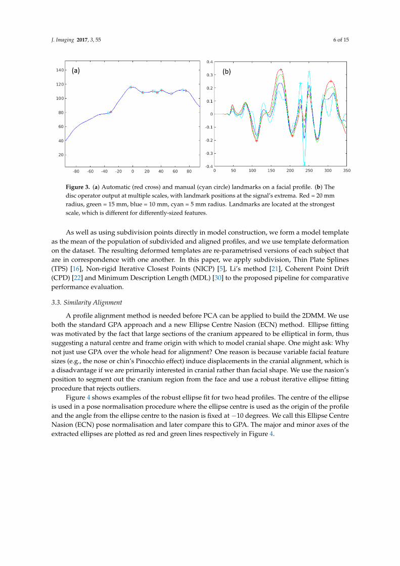
The operator is very easily adapted to multiple scales, with smaller scales being straightforwardsubsamples of the disc points [xd, yd] at larger scales. In this case, we reapply Equation (3) to thesubsample and, as with the larger scale, apply a low pass filter. A useful property of the operator,in contrast to a standard curvature operator, is that its scale is easily tuned to the size of the featuresthat one is interested in: we use a 20-mm disc radius for most profile landmarks (nasion, pronasale,subnasale, chin concavity and pogonion), except those around the lips (upper lip, lower lips, centreof lips), where we use the smallest scale, 5 mm. Figure 3 illustrates the disc operator’s output at fourscales to illustrate its behaviour. For five of eight facial profile landmarks, the strongest output is(usually) the largest scale. For the remaining three, the strongest output is the smallest scale.

The landmarking algorithm employed finds the nearest strong local extrema of the appropriatesign and at the appropriate scale. We first refine the pogonion (chin), subnasale, pronasale (nose tip)and nasion at the largest operator scale. We then consider upper, centre and lower lips simultaneouslyby looking for a strong M-shaped disc operator signature at the smallest scale (5 mm, cyan, in Figure 3),between the subnasale and pogonion. Finally, we find the chin cleft location as the strongest minimumbetween the lower lip and pogonion.

3.2. Correspondence Establishment

To extract profile points using subdivision, we have an interpolation procedure that ensures thatthere is a fixed number of evenly-spaced points between any pair of facial profile landmarks. However,it is not possible to landmark the cranial region and extract profile model points in the same way.This area is smooth and approximately elliptical in structure, and so, we project vectors from the ellipsecentre and intersect a set of fitted cubic spline curves, starting at the nasion and incrementing the angleanticlockwise in small steps (we use one degree) over a fixed angle.

J. Imaging 2017, 3, 55 6 of 15

Figure 3. (a) Automatic (red cross) and manual (cyan circle) landmarks on a facial profile. (b) Thedisc operator output at multiple scales, with landmark positions at the signal’s extrema. Red = 20 mmradius, green = 15 mm, blue = 10 mm, cyan = 5 mm radius. Landmarks are located at the strongestscale, which is different for differently-sized features.

As well as using subdivision points directly in model construction, we form a model templateas the mean of the population of subdivided and aligned profiles, and we use template deformationon the dataset. The resulting deformed templates are re-parametrised versions of each subject thatare in correspondence with one another. In this paper, we apply subdivision, Thin Plate Splines(TPS) [16], Non-rigid Iterative Closest Points (NICP) [5], Li’s method [21], Coherent Point Drift(CPD) [22] and Minimum Description Length (MDL) [30] to the proposed pipeline for comparativeperformance evaluation.

3.3. Similarity Alignment

A profile alignment method is needed before PCA can be applied to build the 2DMM. We useboth the standard GPA approach and a new Ellipse Centre Nasion (ECN) method. Ellipse fittingwas motivated by the fact that large sections of the cranium appeared to be elliptical in form, thussuggesting a natural centre and frame origin with which to model cranial shape. One might ask: Whynot just use GPA over the whole head for alignment? One reason is because variable facial featuresizes (e.g., the nose or chin’s Pinocchio effect) induce displacements in the cranial alignment, which isa disadvantage if we are primarily interested in cranial rather than facial shape. We use the nasion’sposition to segment out the cranium region from the face and use a robust iterative ellipse fittingprocedure that rejects outliers.

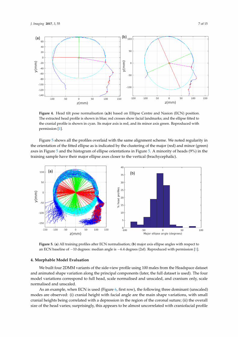
Figure 4 shows examples of the robust ellipse fit for two head profiles. The centre of the ellipseis used in a pose normalisation procedure where the ellipse centre is used as the origin of the profileand the angle from the ellipse centre to the nasion is fixed at −10 degrees. We call this Ellipse CentreNasion (ECN) pose normalisation and later compare this to GPA. The major and minor axes of theextracted ellipses are plotted as red and green lines respectively in Figure 4.

J. Imaging 2017, 3, 55 7 of 15

Figure 4. Head tilt pose normalisation (a,b) based on Ellipse Centre and Nasion (ECN) position.The extracted head profile is shown in blue; red crosses show facial landmarks; and the ellipse fitted tothe cranial profile is shown in cyan. Its major axis is red, and its minor axis green. Reproduced withpermission [1].

Figure 5 shows all the profiles overlaid with the same alignment scheme. We noted regularity inthe orientation of the fitted ellipse as is indicated by the clustering of the major (red) and minor (green)axes in Figure 5 and the histogram of ellipse orientations in Figure 5. A minority of heads (9%) in thetraining sample have their major ellipse axes closer to the vertical (brachycephalic).

Figure 5. (a) All training profiles after ECN normalisation; (b) major axis ellipse angles with respect toan ECN baseline of −10 degrees: median angle is −6.4 degrees (2sf). Reproduced with permission [1].

4. Morphable Model Evaluation

We built four 2DMM variants of the side-view profile using 100 males from the Headspace datasetand animated shape variation along the principal components (later, the full dataset is used). The fourmodel variations correspond to full head, scale normalised and unscaled, and cranium only, scalenormalised and unscaled.

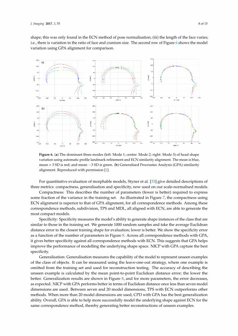
As an example, when ECN is used (Figure 6, first row), the following three dominant (unscaled)modes are observed: (i) cranial height with facial angle are the main shape variations, with smallcranial heights being correlated with a depression in the region of the coronal suture; (ii) the overallsize of the head varies; surprisingly, this appears to be almost uncorrelated with craniofacial profile

J. Imaging 2017, 3, 55 8 of 15

shape; this was only found in the ECN method of pose normalisation; (iii) the length of the face varies;i.e., there is variation in the ratio of face and cranium size. The second row of Figure 6 shows the modelvariation using GPA alignment for comparison.

Figure 6. (a) The dominant three modes (left: Mode 1; centre: Mode 2; right: Mode 3) of head shapevariation using automatic profile landmark refinement and ECN similarity alignment. The mean is blue,mean + 3 SD is red; and mean −3 SD is green. (b) Generalised Procrustes Analysis (GPA) similarityalignment. Reproduced with permission [1].

For quantitative evaluation of morphable models, Styner et al. [33] give detailed descriptions ofthree metrics: compactness, generalisation and specificity, now used on our scale-normalised models.

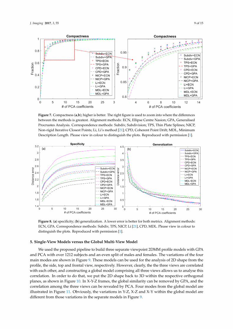
Compactness: This describes the number of parameters (fewer is better) required to expresssome fraction of the variance in the training set. As illustrated in Figure 7, the compactness usingECN alignment is superior to that of GPA alignment, for all correspondence methods. Among thesecorrespondence methods, subdivision, TPS and MDL, all aligned with ECN, are able to generate themost compact models.

Specificity: Specificity measures the model’s ability to generate shape instances of the class that aresimilar to those in the training set. We generate 1000 random samples and take the average Euclideandistance error to the closest training shape for evaluation; lower is better. We show the specificity erroras a function of the number of parameters in Figure 8. Across all correspondence methods with GPA,it gives better specificity against all correspondence methods with ECN. This suggests that GPA helpsimprove the performance of modelling the underlying shape space. NICP with GPA capture the bestspecificity.

Generalisation: Generalisation measures the capability of the model to represent unseen examplesof the class of objects. It can be measured using the leave-one-out strategy, where one example isomitted from the training set and used for reconstruction testing. The accuracy of describing theunseen example is calculated by the mean point-to-point Euclidean distance error; the lower thebetter. Generalization results are shown in Figure 8, and for more parameters, the error decreases,as expected. NICP with GPA performs better in terms of Euclidean distance once less than seven modeldimensions are used. Between seven and 20 model dimensions, TPS with ECN outperforms othermethods. When more than 20 model dimensions are used, CPD with GPA has the best generalizationability. Overall, GPA is able to help more successfully model the underlying shape against ECN for thesame correspondence method, thereby generating better reconstructions of unseen examples.

J. Imaging 2017, 3, 55 9 of 15

Figure 7. Compactness (a,b); higher is better. The right figure is used to zoom into where the differencesbetween the methods is greatest. Alignment methods: ECN, Ellipse Centre Nasion; GPA, GeneralisedProcrustes Analysis. Correspondence methods: Subdiv, Subdivision; TPS, Thin Plate Splines; NICP,Non-rigid Iterative Closest Points; Li, Li’s method [21]; CPD, Coherent Point Drift; MDL, MinimumDescription Length. Please view in colour to distinguish the plots. Reproduced with permission [1].

Figure 8. (a) specificity; (b) generalization. A lower error is better for both metrics. Alignment methods:ECN, GPA. Correspondence methods: Subdiv, TPS, NICP, Li [21], CPD, MDL. Please view in colour todistinguish the plots. Reproduced with permission [1].

5. Single-View Models versus the Global Multi-View Model

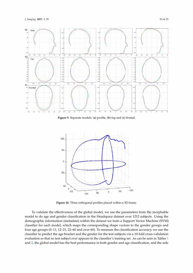
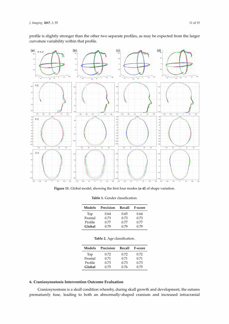
We used the proposed pipeline to build three separate viewpoint 2DMM profile models with GPAand PCA with over 1212 subjects and an even split of males and females. The variations of the fourmain modes are shown in Figure 9. These models can be used for the analysis of 2D shape from theprofile, the side, top and frontal view, respectively. However, clearly, the the three views are correlatedwith each other, and constructing a global model comprising all three views allows us to analyse thiscorrelation. In order to do that, we put the 2D shape back to 3D within the respective orthogonalplanes, as shown in Figure 10. In X-Y-Z frames, the global similarity can be removed by GPA, and thecorrelation among the three views can be revealed by PCA. Four modes from the global model areillustrated in Figure 11. Obviously, the variations in Y-Z, X-Z and X-Y within the global model aredifferent from those variations in the separate models in Figure 9.

J. Imaging 2017, 3, 55 10 of 15

Figure 9. Separate models: (a) profile, (b) top and (c) frontal.

Figure 10. Three orthogonal profiles placed within a 3D frame.

To validate the effectiveness of the global model, we use the parameters from the morphablemodel to do age and gender classification in the Headspace dataset over 1212 subjects. Using thedemographic information (metadata) within the dataset we train a Support Vector Machine (SVM)classifier for each model, which maps the corresponding shape vectors to the gender groups andfour age groups (0–11, 12–21, 22–60 and over 60). To measure the classification accuracy, we use theclassifier to predict the age bracket and the gender for the test subjects via a 10-fold cross-validationevaluation so that no test subject ever appears in the classifier’s training set. As can be seen in Tables 1and 2, the global model has the best performance in both gender and age classification, and the side

J. Imaging 2017, 3, 55 11 of 15

profile is slightly stronger than the other two separate profiles, as may be expected from the largercurvature variability within that profile.

Figure 11. Global model, showing the first four modes (a–d) of shape variation.

Table 1. Gender classification.

Models Precision Recall F-score

Top 0.64 0.65 0.64Frontal 0.73 0.73 0.73Profile 0.77 0.77 0.77Global 0.79 0.79 0.79

Table 2. Age classification.

Models Precision Recall F-score

Top 0.72 0.72 0.72Frontal 0.71 0.71 0.71Profile 0.73 0.73 0.73Global 0.75 0.76 0.75

6. Craniosynostosis Intervention Outcome Evaluation

Craniosynostosis is a skull condition whereby, during skull growth and development, the suturesprematurely fuse, leading to both an abnormally-shaped cranium and increased intracranial

J. Imaging 2017, 3, 55 12 of 15

pressure [34]. We present a case study of 25 craniosynostosis patients (all boys), 14 of which haveundergone one type of corrective procedure called Barrel Staving (BS) and the other 11, anothercorrective procedure called Total Calvarial Remodelling (TCR). The intervention aim is to remodel thepatient’s skull shape towards that of an adult, and we can employ our model in assessing this.

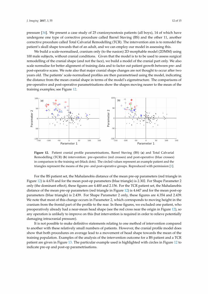
We build a scale-normalised, cranium only (to the nasion) 2D morphable model (2DMM) using100 male subjects, without cranial conditions. Given that the model is to to be used to assess surgicalremodelling of the cranial shape (and not the face), we build a model of the cranial part only. We alsoscale normalise for better alignment of training data and to factor out patient growth between pre- andpost-operative scans. We note also that major cranial shape changes are not thought to occur after twoyears old. The patients’ scale-normalised profiles are then parametrised using the model, indicatingthe distance from the mean cranial shape in terms of the model’s eigenstructure. The comparisons ofpre-operative and post-operative parametrisations show the shapes moving nearer to the mean of thetraining examples; see Figure 12.

Figure 12. Patient cranial profile parametrisations, Barrel Staving (BS) (a) and Total CalvarialRemodelling (TCR) (b) intervention: pre-operative (red crosses) and post-operative (blue crosses)in comparison to the training set (black dots). The circled values represent an example patient and thetriangles represent the means of the pre- and post-operative groups. Reproduced with permission [1].

For the BS patient set, the Mahalanobis distance of the mean pre-op parameters (red triangle inFigure 12) is 4.670 and for the mean post-op parameters (blue triangle) is 2.302. For Shape Parameter 2only (the dominant effect), these figures are 4.400 and 2.156. For the TCR patient set, the Mahalanobisdistance of the mean pre-op parameters (red triangle in Figure 12) is 4.647 and for the mean post-opparameters (blue triangle) is 2.439. For Shape Parameter 2 only, these figures are 4.354 and 2.439.We note that most of this change occurs in Parameter 2, which corresponds to moving height in thecranium from the frontal part of the profile to the rear. In these figures, we excluded one patient, whopreoperatively already had a near-mean head shape (see the red cross near the origin in Figure 12), soany operation is unlikely to improve on this (but intervention is required in order to relieve potentiallydamaging intracranial pressure).

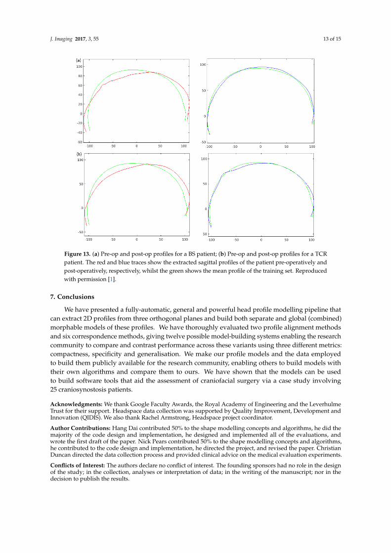
It is not possible to make definitive statements relating to one method of intervention comparedto another with these relatively small numbers of patients. However, the cranial profile model doesshow that both procedures on average lead to a movement of head shape towards the mean of thetraining population. Examples of the analysis of the intervention outcome for a BS patient and a TCRpatient are given in Figure 13. The particular example used is highlighted with circles in Figure 12 toindicate pre-op and post-op parametrisations.

J. Imaging 2017, 3, 55 13 of 15

Figure 13. (a) Pre-op and post-op profiles for a BS patient; (b) Pre-op and post-op profiles for a TCRpatient. The red and blue traces show the extracted sagittal profiles of the patient pre-operatively andpost-operatively, respectively, whilst the green shows the mean profile of the training set. Reproducedwith permission [1].

7. Conclusions

We have presented a fully-automatic, general and powerful head profile modelling pipeline thatcan extract 2D profiles from three orthogonal planes and build both separate and global (combined)morphable models of these profiles. We have thoroughly evaluated two profile alignment methodsand six correspondence methods, giving twelve possible model-building systems enabling the researchcommunity to compare and contrast performance across these variants using three different metrics:compactness, specificity and generalisation. We make our profile models and the data employedto build them publicly available for the research community, enabling others to build models withtheir own algorithms and compare them to ours. We have shown that the models can be usedto build software tools that aid the assessment of craniofacial surgery via a case study involving25 craniosynostosis patients.

Acknowledgments: We thank Google Faculty Awards, the Royal Academy of Engineering and the LeverhulmeTrust for their support. Headspace data collection was supported by Quality Improvement, Development andInnovation (QIDIS). We also thank Rachel Armstrong, Headspace project coordinator.

Author Contributions: Hang Dai contributed 50% to the shape modelling concepts and algorithms, he did themajority of the code design and implementation, he designed and implemented all of the evaluations, andwrote the first draft of the paper. Nick Pears contributed 50% to the shape modelling concepts and algorithms,he contributed to the code design and implementation, he directed the project, and revised the paper. ChristianDuncan directed the data collection process and provided clinical advice on the medical evaluation experiments.

Conflicts of Interest: The authors declare no conflict of interest. The founding sponsors had no role in the designof the study; in the collection, analyses or interpretation of data; in the writing of the manuscript; nor in thedecision to publish the results.

J. Imaging 2017, 3, 55 14 of 15

References

1. Dai, H.; Pears, N.; Duncan, C. A 2D morphable model of craniofacial profile and its application tocraniosynostosis. In Proceedings of the Annual Conference on Medical Image Understanding and Analysis,Edinburgh, UK, 11–13 July 2017; pp. 731–742.

2. Blanz, V.; Thomas, V. A morphable model for the synthesis of 3D faces. In Proceedings of the 26th AnnualConference on Computer Graphics and Interactive Techniques, Los Angeles, CA, USA, 8–13 August 1999;pp. 187–194.

3. Blanz, V.; Thomas, V. Face recognition based on fitting a 3D morphable model. IEEE Trans. Pattern Anal.Mach. Intell. 2003, 25, 1063–1074.

4. Paysan, P.; Reinhard, K.; Brian, A.; Sami, R.; Thomas, V. A 3D face model for pose and illumination invariantface recognition. In Proceedings of the 2009 6th IEEE International Conference on Advanced Video andSignal Based Surveillance, Genoa, Italy, 2–4 September 2009; pp. 296–301.

5. Amberg, B.; Sami, R.; Thomas, V. Optimal step nonrigid icp algorithms for surface registration.In Proceedings of the IEEE Conference on Computer Vision and Pattern Recognition, Minneapolis, MN,USA, 17–22 June 2007.

6. Booth, J.; Ponniah, A.; Dunaway, D.; Zafeiriou, S. Large Scale Morphable Models. IJCV 2017,doi:10.1007/s11263-017-1009-7.

7. Arun, K.; Huang T.S.; Blostein, S.D. Least squares fitting of two 3D point sets. IEEE Trans. Pattern Anal.Mach. Intell. 1987, 9, 698–700.

8. Besl, P.J.; Neil, D.M. A method for registration of 3-D shapes. IEEE Trans. Pattern Anal. Mach. Intell. 1992, 14,239–256.

9. Booth, J.; Roussos, A.; Zafeiriou, S.; Ponniah, A.; Dunaway, D. A 3d morphable model learnt from 10,000 faces.In Proceedings of the IEEE Conference on Computer Vision and Pattern Recognition, Las Vegas, NV, USA,27–30 June 2016; pp. 5543–5552.

10. Hontani, H.; Matsuno, T.; Sawada, Y. Robust nonrigid ICP using outlier-sparsity regularization.In Proceedings of the IEEE Conference on Computer Vision and Pattern Recognition, Providence, RI,USA, 16–21 June 2012; pp. 174–181.

11. Cheng, S.; Marras, I.; Zafeiriou, S.; Pantic, M. Active nonrigid ICP algorithm. In Proceedings of the 2015 11thIEEE International Conference and Workshops on Automatic Face and Gesture Recognition (FG), Ljubljana,Slovenia, 4–8 May 2015; Volume 1, pp. 1–8.

12. Cheng, S.; Marras, I.; Zafeiriou, S.; Pantic, M. Statistical non-rigid ICP algorithm and its application to 3Dface alignment. Image Vis. Comput. 2017, 58, 3–12.

13. Kou, Q.; Yang, Y.; Du, S.; Luo, S.; Cai, D. A modified non-rigid icp algorithm for registration of chromosomeimages. In Proceedings of the International Conference on Intelligent Computing, Lanzhou, China,2–5 August 2016; pp. 503–513.

14. Dai, H.; Pears, N.; Smith, W.; Duncan, C. A 3d morphable model of craniofacial shape and texture variation.In Proceedings of the International Conference on Computer Vision, Venice, Italy, 22–29 October 2017;Volume 1, p. 3.

15. Dai, H.; Smith, W.A.; Pears, N.; Duncan, C. Symmetry-factored Statistical Modelling of Craniofacial Shape.In Proceedings of the International Conference on Computer Vision Venice, Italy, 22–29 October 2017;pp. 786–794.

16. Bookstein, F.L. Principal warps: Thin-plate splines and the decomposition of deformations. IEEE Trans.Pattern Anal. Mach. Intell. 1989, 11, 567–585.

17. Yang, J. The thin plate spline robust point matching (TPS-RPM) algorithm: A revisit. Pattern Recognit. Lett.2011, 32, 910–918.

18. Lee, A.X.; Goldstein, M.A.; Barratt, S.T.; Abbeel, P. A non-rigid point and normal registration algorithm withapplications to learning from demonstrations. In Proceedings of the 2015 IEEE International Conference onRobotics and Automation (ICRA), Seattle, WA, USA, 26–30 May 2015; pp. 935–942.

19. Lee, J.H.; Won, C.H. Topology preserving relaxation labeling for nonrigid point matching. IEEE Trans. PatternAnal. Mach. Intell. 2011, 33, 427–432.

J. Imaging 2017, 3, 55 15 of 15

20. Ma, J.; Zhao, J.; Jiang, J.; Zhou, H. Non-Rigid Point Set Registration with Robust Transformation Estimationunder Manifold Regularization. In Proceedings of the Thirty-First AAAI Conference on Artificial Intelligence,San Francisco, CA, USA, 4–9 February 2017; pp. 4218–4224.

21. Li, H.; Robert, W.S.; Mark, P. Global Correspondence Optimization for Non-Rigid Registration of DepthScans. Comput. Graph. Forum 2008, 27, doi:10.1111/j.1467-8659.2008.01282.x.

22. Myronenko, A.; Song, X. Point set registration: Coherent point drift. IEEE Trans. Pattern Anal. Mach. Intell.2010, 32, 2262–2275.

23. Cootes, T.F.; Gareth, J.E.; Christopher, J.T. Active appearance models. IEEE Trans. Pattern Anal. Mach. Intell.2001, 23, 681–685.

24. Wiskott, L.; Krüger, N.; Kuiger, N.; Von Der Malsburg, C. Face recognition by elastic bunch graph matching.IEEE Trans. Pattern Anal. Mach. Intell. 1997, 19, 775–779.

25. Sauer, P.; Cootes, T.F.; Taylor, C.J. Accurate regression procedures for active appearance models.In Proceedings of the British Machine Vision Conference, Dundee, UK, 29 August–2 September 2011.

26. Tresadern, P.A.; Sauer, P.; Cootes, T.F. Additive update predictors in active appearance models. In Proceedingsof the British Machine Vision Conference, Aberystwyth, UK, 31 August–3 September 2010.

27. Smith, B.M.; Zhang, L. Joint face alignment with nonparametric shape models. In Proceedings of the 12thEuropean Conference on Computer Vision, Florence, Italy, 7–13 October 2012.

28. Zhou, F.; Brandt, J.; Lin, Z. Exemplar-based graph matching for robust facial landmark localization.In Proceedings of the 14th IEEE International Conference on Computer Vision, Sydney, Australia,1–8 December 2013.

29. Zhu, X.; Ramanan, D. Face detection, pose estimation, and landmark localization in the wild. In Proceedingsof the Computer Vision and Pattern Recognition, Providence, RI, USA, 16–21 June 2012.

30. Davies, R.H.; Twining, C.J.; Cootes, T.F.; Waterton, J.C.; Taylor, C.J. A minimum description length approachto statistical shape modeling. IEEE Trans. Med. Imag. 2002, 21, 525–537.

31. Viola, P.; Michael, J.J. Robust real-time face detection. Int. J. Comput. Vis. 2004, 57, 137–154.32. Asthana, A.; Zafeiriou, S.; Cheng, S.; Pantic, M. Robust discriminative response map fitting with constrained

local models. In Proceedings of the IEEE Conference on Computer Vision and Pattern Recognition, Portland,OR, USA, 23–28 June 2013.

33. Styner, .A.M.; Kumar, T.R.; Lutz-Peter, N.; Gabriel, Z.; Gábor, S.; Christopher, J.T.; Rhodri, H.D. Evaluation of3d correspondence methods for model building. Inf. Process. Med. Imag. 2003, 18, 63–75.

34. Robertson, B.; Dai, H.; Pears, N.; Duncan, C. A morphable model of the human head validating theoutcomes of an age-dependent scaphocephaly correction. Int. J. Oral Maxillofac. Surg. 2017, 46, 68,doi:10.1016/j.ijom.2017.02.248.

c© 2017 by the authors. Licensee MDPI, Basel, Switzerland. This article is an open accessarticle distributed under the terms and conditions of the Creative Commons Attribution(CC BY) license (http://creativecommons.org/licenses/by/4.0/).