Embed Size (px)
Citation preview

MODELLING OF PROTEIN SOLUTION PROPERTIES
A Thesis submitted to the University of London
for the degree of Doctor of Philosophy
by
Sabine M. Agena, M.Sc., Dipl.-Ing.
Department of Chemical & Biochemical Engineering
University College London
London, UK
November 1997

This thesis is dedicated with much love
to my husband Amit and
to my parents Gabriele and Helmut

Abstract
Abstract
The research pursued in this work concentrates on modelling two protein solution
properties: activity coefficients and solubility. While modelling protein solubility
was the prime objective activity coefficients were considered first as deviation from
ideal solution behaviour was expected to occur for protein containing systems.
Activity coefficients of protein related compounds, amino acids and peptides, were
studied first hypothesising that these compounds represent proteins and because
activity coefficient data is documented for those compounds but not for proteins. The
predictive UNIFAC model was studied but failed, which led to examination of the
related UNIQUAC model. The objective of the work was the creation of a model
base, which was achieved. This model base was then utilised for protein containing
systems.
Protein activity coefficient data was made available and could be successfully
Page 3
Abstract
modelled using the established framework. Furthermore, the activity coefficient data
was examined over different pH and temperature ranges, salt types and
concentrations. A qualitative comparison of the data to protein solubility results of
other researchers was pursued and used to confirm the model approach.
Having demonstrated that protein solubility was qualitatively represented through
protein activity coefficients a quantitative solubility approach was addressed next.
For two protein systems the solubility behaviour was modelled successfully as a
function of salt concentration and temperature. Findings of other researchers were
integrated into the discussion of the model results while also the calculated protein
activity coefficients were examined and a qualitative confirmation of the model was
achieved.
The models used in this study for the description of two protein solution properties,
when applied to six different proteins over various pH and temperature ranges, salt
types and concentrations showed qualitative and quantitative success. They should
find application to many other protein systems.
Page 4

Acknowledgements
Acknowledgements
I would like to express my sincere gratitude to all those who provided support
throughout my work at University College London, UK and at National Aeronautics
and Space Administration, USA.
Special thanks go to Dr. D. Bogle at U.C.L. and to Dr. M. Pusey at NASA for
supporting me and my work. I would like to thank Dr. D. Bogle for advising me
during my Ph.D. program and for arranging a European research project in which I
participated for two years. Furthermore, I am very grateful to Dr. M. Pusey who
invited me to join his Biophysics research team and supported the final year of this
work.
Furthermore, I would like to thank the team members of our European Union Project
in the United Kingdom, Denmark, Austria and Spain for their co-operation and
hospitality. Moreover, I like to thank Dr. L. Constantinou, Prof. R. Gani and Prof. P.
Page 5

Acknowtedements
Rasmussen in Denmark for inviting me to their department and for their support.
Special thanks go also to Prof. F. Pessoa from Brazil for many interesting
discussions. Last, I like to thank Prof. D. Winzor, Prof. P. Wills, Prof. A. Lenhoff
and Prof. H. Blanch who took the time to discuss my work.
Furthermore, I am very grateful to the European Union who granted me a personal
research fellowship to pursue part of this work.
Page 6

Table of Contents
Table of Contents
Abstract
3
Acknowledgements
5
Table of Contents
7
List of Tables
11
List of Figures
16
Chapter 1 Modelling of Protein Solution Properties
19
1.1 Introduction
19
Chapter 2 Theoretical Background
32
2.1 Introduction
32
2.2 Characterisation of Proteins
33
2.3 Activity Coefficients and Standard States
43
2.4 The Original UNIQUAC Model_______ 46
Page 7

Table of Contm
2.5 The Original UNIFAC Model
52
2.6 The Modified Model ______ 56
2.7 Appraisal of the Models ____ 58
2.8 Summary _______________ 62
2.9 Nomenclature - 63
Chapter 3 Calculation of Amino Acid and Peptide Activity Coefficients___________ 66
3.1 Introduction 66
3.2 Activity Coefficient Data_______________________________________________ 68
3.3 Study of the UNIFAC and UNIQUAC Models ___________________________ 70
3.3.1 Study of the UNIFAC Model _______________________________________ 71
3.3.2 Study of the UNIQUAC Model___________________________________ 83
3.4 Summary 89
3.5 Nomenclature __________________________________________ 90
Chapter 4 Calculation of Protein Activity Coefficients
92
4.1 Introduction ________________________________ 92
4.2 Activity Coefficient Data____________________ 94
4.2.1 Virial Expansion _____________________ 96
4.3 Study of the Original UNIQUAC Model _______ 100
Page 8

Table of Contents
4.4 Summary
119
4.5 Nomenclature
120
Chapter 5 Calculation of Protein Solubility
123
5.1 Introduction ________________________ 123
5.2 Experimental Solubility Data________ 125
5.3 Solid - Liquid Equilibrium Model
130
5.4 Study of the Solubility Model _______ 136
5.5 Summary _____________________ 147
5.6 Nomenclature
148
Chapter 6 Conclusions
150
Chapter 7 Future Research Objectives
168
Appendix A Activity Coefficient Data of Amino Acids and Peptides
180
Appendix B FORTRAN Code of the IJNIQUAC Model (unsymmetric)
183
Appendix C Activity Coefficient Data of Proteins _____________________________ 213
Page 9

Table of Contents
Appendix D Solubility Data of Proteins
220
Appendix E FORTRAN Code of the Solubility Model
227
References
259
Page 10

List of Tables
List of Tables
Table 1.1: Biochemical unit operations and the exploited protein properties _________ 23
Table 2.2.1.: Molecular structure and characterisation of the twenty amino acid
residues
34
Table 2.2.2: lonised amino acid groups and their P'a and reaction_________________ 37
Table 2.4.1: The combinatorial term and residual term expressions for activity
coefficient calculations using the original UNIQUAC model _____________________ 51
Table 3.3.1.1: Molecular structures of amino acids and peptides and their UNIFAC
groups 72
Page 11

List of Tables
Table 3.3.1.2: Performance of the activity coefficient calculations for amino acids
and peptides using various IJNIFAC model versions
74
Table 3.3.2.1: Structural parameters and binary interaction parameters for glycine,
proline, glycylglycine and water
85
Table 3.3.2.2: Performance of the activity coefficient calculations for glycine, proline
and glycylglycine using the original UNIQUAC model (unsymmetric) ____________ 85
&4i&&
Table 3.3.2.3: Experirncntation error evaluation using two sets of experimentally
determined activity coefficient data for glycine, proline and glycylglycine __________ 87
Table 4.2.1: Protein systems and system conditions investigated ____________________ 95
Table 4.2.1.1: Virial expansion data of protein systems
99
Table 4.3.1: Calculated van der Waals volumes and surface areas of proteins _______ 103
Table 4.3.2: UNIQUAC modelling data for protein systems____________________ 108
Page 12

List of Tables
Table 4.3.3: Performance of protein activity coefficient calculations using the
original UNIQUAC model (unsymmetric)
112
Table 5.2.1: Protein systems and system conditions investigated ________________ 126
Table 5.3.1: Structural parameters of proteins, salt ions and pseudo solvents_______ 134
Table 5.4.1: Parameters of the thermodynamic solubility product for lysozyme and
concanavalin A
137
Table 5.4.2: Binary interaction parameters for the lysozyme system _____________ 139
Table 5.4.3: Binary interaction parameters for the concanavalin A system__________ 139
Table 5.4.4: Performance of solubility calculations for lysozyme and concanavalin A
using the solid - liquid equilibrium model
145
Table A. 1: Experimentally determined activity coefficients of amino acids as a
function of composition 181
Page 13

List of Tables
Table A.2: Experimentally determined activity coefficients of peptides as a function of
composition
182
Table C. 1: Experimentally determined activity coefficients of serum albumin, S, as a
function of composition
214
Table C.2: Experimentally determined activity coefficients of a - chymotrypsin, Cl, as
a function of composition
215
Table C.3: Experimentally determined activity coefficients of a - chymotrypsin, C2, as
afunction of composition __________________________________________________ 215
Table C.4: Experimentally determined activity coefficients of a - chymotrypsin, C3, as
a function of composition 216
Table C.5: Experimentally determined activity coefficients of a - chymotrypsin, C4, as
a function of composition 216
Table C.6: Experimentally determined activity coefficients of a - chymotrypsin, CS, as
a function of composition 217
Page 14

List of Tables
Table C.7: Experimentally determined activity coefficients of a - chymotrypsin, C6, as
a function of composition 217
Table C.8: Experimentally determined activity coefficients of a - chymotrypsin, C7, as
afunction of composition _________________________________________________ 218
Table C.9: Experimentally determined activity coefficients of J3 - lactoglobulin, L, as a
function of composition 218
Table C.1O: Experimentally determined activity coefficients of ovalbumin, 0, as a
function of composition 219
Table D. 1: Experimental solubility data of lysozyme, LYS, as a function of
composition and temperature 221
Table D.2: Experimental solubility data of concanavalin A, CON, as a function of
compositionand temperature ______________________________________________ 224
Page 15

List of Figures
List of Figures
Figure 3.3.1 .1: Experimentally determined and modelled (original IINTFAC
unsymmetric) activity coefficients of glycine and proline against the amino acid and
peptide mole fraction
79
Figure 3.3.2.1: Experimentally determined and modelled (original UNIQUAC
unsymmetric) activity coefficients of glycine, proline and glycyiglycine against
theamino acid and peptide mole fraction _____________________________________ 86
Figure 4.2.1 .1: Reduced osmotic pressure of the serum albumin system against
protein concentration
98
Figure 4.3.1: The structural parameters of lysozyme, serum albumin, a -
chymotrypsin and 3 - lactoglobulin against their molecular weight ______________ 107
Page 16

List of Figures
Figure 4.3.2: Programming structure used to determine interaction parameters _____ 110
Figure 4.3.3: Experimentally determined and modelled (original UNIQUAC
unsymmetric) activity coefficients of a - chymotrypsin with varying ionic strength of
potassium sulphate against protein mole fraction
114
Figure 4.3.4: Experimentally determined and modelled (original UNIQUAC
unsymmetric) activity coefficients of a - chymotrypsin with varying pH and salt
types against protein mole fraction 115
Figure 4.3.5: Experimentally determined and modelled (original UNIQUAC
imsymmetric) activity coefficients for a - chymotrypsin at different temperatures
against protein mole fraction 116
Figure 5.2.1: Experimental solubility of lysozyme at various sodium chloride
concentrations against temperature 128
Figure 5.2.2: Experimental solubility of concanavalin A at various ammonium
sulphate concentrations against temperature ___________________________________ 129
Page 17

List of Figures
Figure 5.3.1: Structure of the solubility model
131
Figure 5.4.1: Experimental and modelled solubility of lysozyme at five different
sodium chloride concentrations against temperature
142
Figure 5.4.2: Experimental and modelled solubility of concanavalin A at different
ammonium sulphate concentrations against temperature
143
Figure 5.4.3: Modelled activity coefficients of lysozyme at different sodium chloride
concentrations against temperature
144
Page 18

Chapter 1 Modelling of Protein Solution Properties
Chapter 1
Modelling of Protein Solution Properties
The motivation for this work is presented and the development and pursuit of the
research project is described while the relevant publications are reviewed
1.1 Introduction
This work concentrates on the modelling of protein solution properties. Proteins were
the targeted compounds as they are a main product range in the rapidly developing
biochemical industry. From biochemical processes various proteins are produced e.g.
enzymes used in washing powders, hormones such as insulin used for medical
purposes and growth hormones used for cattle breeding.
Page 19

Chapter 1 Modelling of Protein Solution Properties
Two kinds of solution properties were studied for different proteins: activity
coefficients and solubility. The process of selecting these protein properties in order
to study and model them are presented in this chapter, chapter one, while also the
overall significance of this work is elaborated.
This work was pursued due to the fact that knowledge of protein solution properties,
either from experiment or from models, is of importance in a variety of areas such as
biochemical process development, protein crystal growth and medical research. The
area of optimal process development, where e.g. product quality, processing cost and
process controllability determine an optimal process, was the main focus for this
work [Bogle et al.,1996] and guided this work. In order to develop optimal
biochemical processes, which is becoming increasingly important due to rising
industrial competition, the properties of the different compounds, i.e., product and
impurities, have to be evaluated. Already the first step towards the optimal process
development, which deals with the selection and arrangement of process units, i.e.,
process synthesis, requires extensive assessment of compound properties. Process
synthesis concepts have been discussed and applied with success for chemical
engineering purposes [Siirola and Rudd, 1971; Barnicki and James, 1990; Jaksland et
al., 1995] but only a few works are aimed at biochemical engineering problems.
Page 20

Chapter 1 Modellingof Protein Solution Properties
Wheelwright (1987) discussed applications of process synthesis concepts for
biochemical processes. He introduced heuristics based on physicochemical
compound properties. Key properties of the product, e.g. protein, and the impurities
have to be screened, and those properties that demonstrate greatest difference for
product and impurities determine, which separation and purification processes are
chosen. Asenjo (1990) introduced an expert system that allows for computer aided
synthesis of biochemical processes. He also introduced a set of heuristic rules to
select process units as a function of physicochemical properties of the different
compounds or systems, e.g. bacterial cells, occurring during processing. In 1996 Wai
et al. studied a related concept using a property ratio matrix to create initial process
alternatives that are likely to lead to the optimal process.
All the mentioned synthesis methodologies require a diverse range of compound
properties as do any of the other process development stages such as process design
and process simulation. The properties needed for these methodologies are most
conveniently obtained from models and it is the aim of this research project to study
models that estimate compound properties over system conditions and predict
properties over different compound types.
Following from the fact that compound properties are needed for the first step, i.e.,
Page 21

Chapter 1 Mode11in of Protein Solution Properties
process synthesis, towards the development of optimal biochemical processes, the
major process units and the relating compound properties exploited in these units
were examined. This was pursued in an attempt to screen the properties for their
importance. Protein production units used in the downstream processing from
homogenisation, solubilisation to freeze - dying were viewed with respect to the
exploited physicochemical properties and are listed in table 1 .1. Depending on the
unit operation different properties are exploited e g. an ion exchange unit is applied
when differences in the ionic surface charges are found at given system conditions
for product and impurities. Likewise, e.g. sedimentation is applied as a separation
step if density and size differences are encountered for product and impurities. The
main physiochemical properties exploited in the most commonly used biochemical
unit operations are: solubility, density, size, molecular weight, partition coefficient,
biospecific attraction, ionic surface charge, hydrophopicity, covalent binding,
isoelectric point, melting point and glass temperature [Wheelwright, 1987; Burgess,
1988; Asenjo, 19901.
The decision to focus on protein solubility followed various reasons: occurrence of
solubility related unit operations in the downstream processing, the availability of
experimental data, and the non availability of an estimation or prediction method.
The fact that protein solubility has been investigated since the mid 19th century
Page 22

Chapter 1 Modelling of Protein Solution Properties
Table 1.1: Biochemical unit operations and the exploited protein properties
biochemical unit operation physicochemical property
solubilisation
sedimentation
centrifugation
filtration
membrane filtration
extraction
partitioning
precipitation
evaporation
bio - reactions
ion exchange
ion exchange chromatography
hydrophobic interaction chromatography
covalent chromatography
affinity chromatography
chromatofocusing
size exclusion chromatography
partitioning chromatography
crystallisation
solubility
density, size
density, size
size
size, molecular weight
partition coefficient
partition coefficient
solubility
vapour pressure*
biospecific attraction
ionic surface charge
ionic surface charge
hydrobicity
covalent binding
biospecific attraction
isoelectric point
size
partition coefficient
solubility, melting point
drying by evaporation of water vapour pressure*
lyophilization glass temperature, vapour pressure*
* solvent
Page 23

Chapter 1 Modelling of Protein Solution PrQperties
[Hofmeister, 1888, and references within; Ducruix and Giege, 1992, and references
within] until today emphasises its importance. The importance to model a protein's
solubility is further demonstrated by the fact that solubility differences of compounds
are exploited in 80 % of the applied isolation procedures [Scopes, 19871 and in 57 %
of the large scale processes [Bonnerjea et al., 1986]. Furthermore, only recently
useful experimental data for protein solubility as a function of salt concentration,
temperature and p1-I [Cacioppo et al., 1991; Ewing Ct at., 1994] was made available,
which therefore allows for comprehensive modelling to be undertaken. Moreover, a
model for protein solubility, that is applicable for process development purposes, is
not yet available.
This work was motivated by the requirements for optimal biochemical process
development where e.g. a solubility model supports the design of a crystallisation
unit or can clarify if a solid and liquid phase are encountered for a certain unit
operation. However, not only engineering and production purposes link up to this
work but also studies aiming at the protein crystal growth process and at medical
research. For the protein crystal process a protein's solubility is a major property
which once it can be modelled or predicted will support the creation of crystals. To
understand a protein's crystallisation process, which is directly related to a protein's
solubility behaviour, and to produce protein crystals is a major research objective of
Page 24

Chapter 1 Modellin2 of Protein Solution Properties
various teams [Ducruix and Giege, 1992, and references within]. Crystals are needed
to determine a protein's three dimensional structure. Knowledge of a protein's three
dimensional structure not only enlightens our understanding of a protein's function
and biological purpose but also guides us when designing drugs.
The three dimensional description for human serum albumin [Carter et al., 1989; He
and Carter, 1992] was established as a result of such crystallisation work. Human
serum albumin carries important drugs such as aspirin in the blood and its structural
information will allow for further and enhanced drug creations and especially for
those drugs that need to be transported via the blood. Creation of the three
dimensional model of canavalin [McPherson and Rich, 1973; McPherson and
Spencer, 1975], a protein found in the jack bean and a major source of protein for
humans and domestic animals, will allow us to produce plants that are more
nutritional arid resistant to pest. Furthermore, protein crystal growth research is
applied to learn how elastase damages lung tissue while general research towards the
medical treatment for cancer, AIDS, diabetes, sickle cell anaemia and rheumatoid
arthritis is supported.
However, a precondition for this kind of work is that protein crystals are obtained but
the crystal growth process is a limiting step. To obtain a crystal long periods of
Page 25

Chapter 1 Modelling of Protein Solution Properties
experimental trials are encountered due to long periods of nucleation and growth
[Blundell and Johnson, 1976; McPherson, 1982], which might last over months. For
the enzyme lysozyme crystallisation periods of well above a month are encountered
when e.g. hexagonal crystals are produced [communication with Pusey, 1997]. A
method to model or even predict crystallisation conditions and therefore a model that
describes protein solubility, is therefore also of great interest in this research area.
This work aims at a model for protein solubility. Models that describe protein
solubility are few. The most well known empirical description of protein solubility
with respect to salts as precipitant agents was introduced by Cohn in 1925 and has
been extensively used and studied by others till today [Green, 1931; Dixon and
Webb, 1961; Foster et al., 1971; Niktari et al., 1989]. In 1977 a theoretically based
model followed. Melander and Horvath (1977) described protein solubility as a
function of salt concentration by relating the solubility behaviour to hydrophobic
effects. But Przybycien and Bailey (1989) showed that this model was not consistent
with their experimental solubility results. Further theoretical models were recently
presented by Chiew et al. (1995) and Kuehner et a!. (1996), who used molecular
thermodynamics to describe salt induced protein precipitation. The models
incorporate different interaction potentials to represent protein solubility and they
succeeded in finding a semi - quantitative agreement with their experimental results.
Page 26

Chapter 1 Modelling of Protein Solution Properties
However, a solubility model is needed that computes quantitatively correctly the
protein solid - liquid equilibrium for a variety of protein systems and has a predictive
potential. Therefore, a semi - empirical model was approached, which had been used
with slight variations for the modelling of the solid - liquid equilibrium of organic
[Gmehling et al., 1978; Nass, 1988; Peres and Marcedo, 1994] and inorganic
compounds [Nicolaisen et al., 1993] but not for proteins. The theoretical framework
adapted for our systems of interest, protein - salt - water, uses the solubility product
to represent the equilibrium of liquid and crystal protein, while a protein's deviation
from ideal solution behaviour is also accounted for.
Proteins have been demonstrated to show high deviations from ideal solution
behaviour [Ross and Minton, 1977], which is expected due to the size difference
encountered between e.g. the protein and solvent molecule, i.e., water. Furthermore,
various different interactions occur for protein molecules, salt ions and water
molecules and create deviation from ideal solution behaviour. Therefore, the
modelling of protein activity coefficients representing the deviation from ideal
solution behaviour due to size difference and interactions was studied here. The only
previous studies aiming at protein activity coefficients are those of Ross and Minton
(1977), who studied sickle cell anaemia by means of activity coefficient examination,
and Wills et al. (1993), who examined the excluded volume contributions for
Page 27
Chapter 1 Modelling of Protein Solution Properties
proteins by interpreting the deduced virial coefficients which also led to activity
coefficient studies. Both teams based their work on the virial expansion, which gives
protein activity coefficients as a function of system composition at constant
temperature and pH. For this work another activity coefficient model was aimed at as
not only activity coefficients over system composition but also over system
temperature had to be expressed while additionally a predictive potential of the
model was an objective.
Activity coefficient models have been derived from Wilsons concept [Wilson, 1964]
to describe solution behaviour by means of local composition, which was developed
from molecular thermodynamic theories [Smith and van Ness, 1987]. For a solution,
local compositions, different from the overall mixture composition, are assumed,
accounting for the short - range order and non - random orientation that result from
differences in molecular size and intermolecular forces. Three local composition
models are notable: the Wilson equation [Wilson, 1964], the Non - Random - Two -
Liquid equation (NRTL) [Renon and Prausnitz, 1968] and UNiversal QUAsi -
Chemical model (UNIQUAC) [Abrams and Prausnitz, 1975].
The third local composition model, UNIQUAC model, was chosen for this work as it
uses a minimal number of parameters compared to the other models and because the
Page 28

Chapter 1 Modelling of Protein Solution Properties
UNIQUAC Functional - group Activity Coefficient model (UNIFAC) [Fredenslund
et al., 1975] was developed from it. The UNIFAC model is used to calculate activity
coefficients from contributions of defined structural molecular groups, which make
up the molecules in solution. This method creates a predictive tool not only over
system conditions as given with the UNIQUAC model but also over different but
related systems, i.e., compounds. The UNIQUAC and UNIFAC methods were
additionally chosen because they describe system composition and temperature.
While proteins had never been studied with local composition models, systems,
mainly hydrocarbons, that bear similarities with the protein - salt ions - water
systems studied here, were examined and have been described with some success
using these approaches.
Various small organic compounds, which share some of the polar properties with
proteins, were described via local composition models including compounds such as
amino acids and peptides [Nass, 1988; Gupta and Heidemann, 1990; Phino et al.,
1994; Peres and Marcedo, 1994], which are the structural building blocks of proteins.
Furthermore, polymers which share size and hydrophobic features with proteins have
been examined with UNIQUAC and UNIFAC related models [Kontogeorgis et al.,
1997, and references within], where the description of the solution behaviour focused
on athermal approaches. Moreover electrolytes, which have ionic charges in common
Page 29

Chapter 1 Modelling of Protein Solution Properties
with proteins, were modelled describing activity coefficients and solubility
[Nicolaisen et al., 1993] using additionally the Debye Htickel law [Debye and
Hückel, 1923; HUckel, 1925, Debye, 19271 to describe the long range interactions of
ions at low salt concentrations. This modelling approach for simple electrolytes is
also of interest as salt ions are compounds occurring in the systems studied here.
Following these facts the IINIQUAC and UNIFAC models and their different
versions were studied here for protein containing systems.
In this work first of all amino acid and peptide systems, which are the building
blocks of proteins, were studied. In a systematic manner different UNIFAC and
UNIQUAC models were applied to model activity coefficients for amino acids and
peptides. This part of the work was used, to clarify if the predictive UNIFAC model
is applicable for protein related compounds and to establish which model version
would be appropriate if at all for proteins. This first part of this work is presented in
chapter three.
In the second part of this work protein activity coefficients were addressed. A
method to obtain protein activity coefficients from osmotic pressure measurements
was studied and the determined activity coefficient data was modelled using a local
composition model. Systems consisting of a protein, salt ions and water were
Page 30

Chapter 1 Modelling of Protein Solution Properties
examined. The model performance for protein activity coefficients over salt
concentration, pH and temperature was studied, while also a qualitative examination
of protein solubility was pursued. This second part of the work is documented in
chapter four.
In the third and final part of this work the directly measurable solution property,
solubility, was investigated. Protein solubility over salt concentration and
temperature was approached and described via the modelling of protein activity
coefficients. This part of the research is presented in chapter five.
Results and discussions are presented and summarised for these three parts. The
relevant theoretical background for this work is presented in the next chapter, chapter
two. Final chapters discuss the overall conclusions and future research projects,
chapters six and seven, respectively.
Page 31

Chapter 2 Theoretical Background
Chapter 2
Theoretical Background
This chapter discusses proteins and their characteristics. Furthermore, it introduces
the major definitions and models that were studied in this work
2.1 Introduction
The modelling of a protein solution property, protein solubility, was aimed at in this
work using activity coefficients. Consequently first of all proteins and their
characteristics are discussed. This is followed by the definitions for activity
coefficients and their two different standard states, the symmetric and unsynimetric
convention. Additionally, the activity coefficient definition with respect to the excess
Page 32

Chapter 2 Theoretical Background
Gibbs energy is introduced leading to the UNIQUAC [Abrams and Prausnitz, 1975]
and UNIFAC [Fredenslund et al., 1975] expressions, which are models used to
describe activity coefficients and solution behaviour as a function of system
composition and temperature. The UNIQUAC and UNIFAC models are introduced
in detail, including the different UNIQUAC and UNIFAC versions examined in this
work. The presented theories are found to some extent in various references
[Prausnitz et a!., 1986; Smith and van Ness, 1987; Nicolaisen, 1994]. The discussion
relating to proteins is found in references such as Creighton (1984) and Lehninger
(1982).
2.2 Characterisation of Proteins
Proteins are macromolecules built from twenty natural occurring amino acids. Table
2.2.1 shows the structures of the different amino acid residues that build a particular
amino acid and are also found in proteins as amino acids are the building blocks of
proteins. These amino acid residues, R, are situated on the following structure to
configure an amino acid:
H2N-CH(RJ-COOH (2.2.1)
Page 33

Chapter 2 Theoretical Background
Table 2.2.1: Molecular structure and characterisation of the twenty amino acid
residues
Amino acid Property Residue lonised formGlycine non - polar -H -
Alanine non - polar -CH3 -
Valine non - polar -CH(CH3)2 -
Leucine non - polar -CH2-CH(CH3)2 -
Isoleucine non - polar -CH(CH3)(CH2(CH3)) -
Phenylalanine non - polar -CH2-C:-CH:-C1-I -I: o I:
(CH)2 :-CHProline non - polar HN-CH-COOH -
(CH2)3
Tryptophan non - polar -CH2-CCH- NH -
C :- CI: o I:
(CH)2:-(CH)2Serine hydroxyl -CH2-OH -
Threonine hydroxyl -CH(OH)(CH3) -
Aspartic acid acidic -CH2-C(=O)(OH) -CH2-C(:-O)(:-O)
Glutamic acid acidic -(CH2)2-C(=O)(OH)
Asparagine amido -CH2-C(—O)-NH2 -
Glutamine amido -(CH2)2-C(0)-NH2 -
Tyrosine basic -C112-C:-CH:-CH -CH2- C:-CH:-CHI: o I: I: o
(CH)2 :-CH-OH (CFI)2:-CH-0Lysine basic -(CH2)4-NH2 -(CH2)4-WH3
Arginine basic -(CH2)3-NH-C(=NH)(NH2) -(CH2),-NH-C(:-NH2)(:-NH2)
Histidine basic -CH2-C=CH-N -CH2-C=CH-NHI II I I:
NH -CII NH :-CHCysteine disuiphide bonds -CH2-SH -CH2-S
Methionine sulphur -CH2-CH2-S-CH3 -
:- partial double bounds, o aromatic
Page 34

Chapter 2 Theoretical Background
For proline the whole structure is given in table 2.2.1 because proline is an imino
acid as opposed to an amino acid.
A protein is created from a number of amino acids which bind under a condensation
reaction resulting in a sequential arrangement:
(-NH-CH(R,j-CO-) (2.2.2)
Following these reactions a peptide or protein is created, which consists of the
backbone as given above, 2.2.2. This backbone is build of units consisting of a planar
peptide bond (-CO-NH-) and a carbon, the a - carbon, from which the particular
amino acid residue sets off. Following the condensation reactions a chain molecule is
created and its left end is defined as the amino terminus:
H2N-CH(R)-CO-... (2.2.3)
while on the other end the carboxyl terminus is found:
-NH-CH(RJ-COOH (2.2.4)
The twenty amino acids that build proteins contribute to the characteristics of
proteins. Therefore the twenty amino acids and their characteristics are discussed
next. However, amino acids do not describe matters of molecule size which have to
be additionally considered for proteins. The amino acids or amino acid residues are
grouped according to their polarity, their charge, their steric flexibility etc.
Page 35

Chapter 2 Theoretical Background
Some amino acids residues have been demonstrated to accept and release protons and
the ionised forms of these residues are given in table 2.2.1 while the acid base
reaction is documented in table 2.2.2. For six residues ionisation occurs depending
on the environment. Aspartic acid and glutamic acid release protons in the acidic pH
region and are referred to as acidic. Argine, lysine, tyrosine, cystein and histidine
(weaker base) are basic. Moreover, the termini are involved in acid base reactions.
The documented ranges for the pK., values for the different ionised groups indicate in
which pH region ionisation occurs e.g. at a pH of five the carboxyl terminus, aspartic
acid and glutamic acid are found predominantly in their base form while all other
residues are predominantly in their acid form. Following these ionisation reactions
proteins are found to be charged molecules, i.e., polyelectrolytes. In strongly acid
solution proteins are positively charged and in strongly alkaline solution they are
negatively charged. Due to this property proteins migrate in an electric field. At a net
charge of zero no migration occurs and the prevailing pH is defined as a protein's
characteristic p1 (isoelectric point).
Following the formation of ionised groups a strong hydrophilic character is observed
while the aliphatic residues participate in hydrophobic interactions. Residues such as
glycine, alanine, valine, leucine and isoleucine, table 2.2.1, exhibit a hydrophobic
character due to their aliphatic molecule structure. Similar to these, methionine
Page 36

Chapter 2 Theoretical Back2round
Table 2.2.2: lonised amino acid groups and their pK. and reaction
Group pKa* Reaction: acid - base + H
carboxyl terminus 3.5 - 4.3
Aspartic acid 3.9 - 4.0
Glutamic acid 4.3 - 4.5
Histidine 6.0 - 7.0
amino terminus 6.8 - 8.0
-COOH -* -000 + H
-COOH - -000 + H
-COOH -^ -000 + W
-NH2 : -C:-NH2 - -NH=C-NH2 + H
-H3N -* -NH2 +W
Cystein
9.0-9.5
Tyrosine
10.0- 10.3 -OH—-O+H
Lysine 10.4-11.1 -H3N—-NH2+H
Arginine 12.0 -C(:-NH2)(:-NH2) -* -C(-NH2)(=NH) +W
* Creighton, 1984
exhibits a non - polar and relatively non - reactive character. The amino acid residues
serine, threonine and tyrosine have hydroxyl groups and support hydrogen bonds.
Asparagine and glutamine, build hydrogen bonds due to their amido groups.
Looking at steric flexibility it is found that glycine due to its small residue is highly
Page 37

Chapter 2 Theoretical Background
flexible and is often found in the bends of proteins while the steric hindered proline
limits protein flexibility. Aromatic groups found in phenylalanine, tyrosine and
tryptophan contribute to hydrophobic behaviour and steric hindrance. For cystein a
very typical characteristic is the creation of disuiphide bonds, which are responsible
for strong intra- and interstrand interactions.
The interactions, which contribute mainly to the specific characteristics and structure
of a protein are the covalent bindings. Covalent linkage of atoms is established by
sharing of electrons. With covalent bonds such as the peptide bonds and the
disuiphide bonds the major characteristics of a protein's structure and therefore
characteristics are settled. An example are disuiphide bindings, which lead with
increasing number to a decrease of a protein's solubility.
London dispersion forces describe short range non - covalent interactions, which also
contribute to a protein's properties. Between all atoms weak interactions occur due to
the distribution of electronic charges and their location. Their movements create
fluctuating dipoles which result in attractive forces between atoms. Repulsion occurs
when the electron orbitals are forced to overlap.
Interactions that are closely related to the dispersion forces are those of permanent
Page 38
Chapter 2 Theoretical Background
dipoles. These can lead to hydrogen bonding. Hydrogen bonding occurs for proteins
between hydrogen atoms and nitrogen atoms or hydrogen atoms and oxygen atoms.
These atoms are involved in dipole moments due to great differences in the electron
density of covalent bonds. Where opposite dipole charges are found attraction occurs,
otherwise repulsion is found.
The ionic bonds, which are established between differently charged groups tend to
bring together parts over large distances while repulsion occurs between ionic groups
of same charge. Ionic bonds are the strongest non - covalent forces but do depend on
the dielectric constant of the solvent as electrostatic interactions are reduced in
solvents with high dielectric constants such as water.
When dealing with proteins another form of interaction has to be considered.
Hydrophobic interactions describe the behaviour of groups not being attracted by
water or polar substances. While polar molecule groups form hydrogen bonds with
water, non - polar groups are not soluble and tend to form hydrophobic clusters
minimising the contact area with polar solvents e.g. water, which is the solvent
proteins are most commonly exposed to. The hydrophobic parts of a protein are
accumulated in the centre while the hydrophilic parts are exposed at the surface to
interact with the polar solvent. Therefore, a compact and dense structure is observed
Page 39

Chapter 2 Theoretical Background
for some proteins and those are referred to as globular proteins. In this work globular
proteins were studied.
Furthermore, aggregation of protein monomers occurs. Dimers or higher order
aggregates are held together by non - covalent forces as described above. During the
course of this work two proteins that occur as dimers were examined for the protein
activity coefficient and solubility modelling work, - lactoglobulin and concanavalin
A.
The described properties and interactions, which result from the molecular structure,
imply the solution behaviour that might occur between proteins and other system
compounds such as water or salt ions. Moreover, the interactions within a protein are
pictured which lead to a protein's very specific three dimensional structure unlike the
random coiling observed for aliphatic polymers.
The described structures, interactions and properties of proteins lead to certain
classifications. The most common classification is achieved by means of molecular
weights which divides the group of proteins into two groups. The low molecular
weight proteins, which are built from only a few amino acids, are referred to as
peptides while the higher molecular weight ones are called proteins. These two
Page 40

Chapter 2 Theoretical Back2round
classes are defined differently with respect to the reference. One definition uses the
number of peptide bonds where a polypeptide with more than fifteen peptide bonds is
considered a protein [Freifelder, 1986]. Other references are found, which give a
definition according to the number of amino acids incorporated or the molecular
weight. Typically proteins have molecular weights of 5000 Da to 200000 Da
[Lehninger, 1982] and the average molecular weight of the amino acid, which is
incorporated into a protein and constitutes the building block of a protein, is about
120 Da [Creighton, 1984].
Furthermore, proteins are classified according to their composition [Elmore, 1986].
Unconjugated and conjugated proteins are referred to. The first class is composed of
only amino acids as discussed here, while the second one has additional molecular
structures which are not amino acids. The group of conjugate proteins is divided into
nucleoproteins, lipoproteins, glycoproteins, chromoproteins in accordance to their
prosthetic groups.
Moreover, certain properties are used to define proteins. A protein's solubility
behaviour allows for yet another categorisation. Albumins (soluble in water and
dilute solutions of salt), globulins (few soluble in water but soluble in dilute salt
solutions), prolamines (insoluble in water but soluble in 50 - 90 % aqueous ethanol),
Page 41

Chapter 2 Theoretical Background
glutelins (insoluble in the mentioned solvents but soluble in dilute solutions of acids
or bases) and scleroproteins (insoluble in most solvents) were defined over the years.
Another widely applied method of classification was established using a protein's
biological function. Such categories are hormones, enzymes, antibodies, structural
proteins etc. Since the first creation of recombinant proteins at around 1972 another
classification evolved differentiating between recombinant and non - recombinant
proteins. Furthermore, classification due to molecular size, amino acid composition,
conformation (helix content), origin and many other factors are known.
In this work six different proteins, serum albumin (horse blood), a - chymotrypsin
(bovine pancreas), - lactoglobulin (bovine milk), ovalbumin (chicken egg),
lysozyme (chicken egg) and concanavalin A (jack bean), were studied. These
proteins originate from a variety of sources as indicated above and have very
different biological functions. The protein a - chymotrypsin is a protease and its
biological function is to hydrolyse peptide bonds of proteins. The protein lysozyme,
which is the smallest protein (14600 Da) studied during the course of this work,
cleaves bacterial cell walls. Lysozyme therefore prevents infections while it is also
applied on the biochemical processing scale as a biochemical tool to disrupt bacterial
cells. The protein serum albumin again has a very different function. It occurs in the
Page 42

Chapter 2 Theoretical Background
blood and regulates its osmotic pressure while it also is a transport vehicle that
delivers other compounds and drugs through the blood stream. Not only the
biological function of the studied proteins differs but also the examined system
conditions differ e.g. pH and temperature ranges. However, all these proteins have in
common that they are globular proteins, i.e., of a compact structure. Furthermore,
they all originate from natural sources that produce them at high amounts, which
makes them available at the quantities and qualities needed for biophysical studies.
Therefore, these six proteins could be studied here in the first place. The two
proteins, 3 - lactoglobulin and concanavalin A, were studied to represent proteins
that are dimers. The protein concanavalin A is the biggest protein studied here with a
molecular weight 102668 Da.
2.3 Activity Coefficients and Standard States
To model a protein's solution properties such as solubility the activity coefficients
have to be addressed. A description of a solution property has to consider the
deviation from ideal solution behaviour which is expressed through activity
coefficients. For protein containing systems deviation from ideal solution behaviour
Page 43
Chapter 2 Theoretical Background
is expected as demonstrated by Ross and Minton (1977) for haemoglobin.
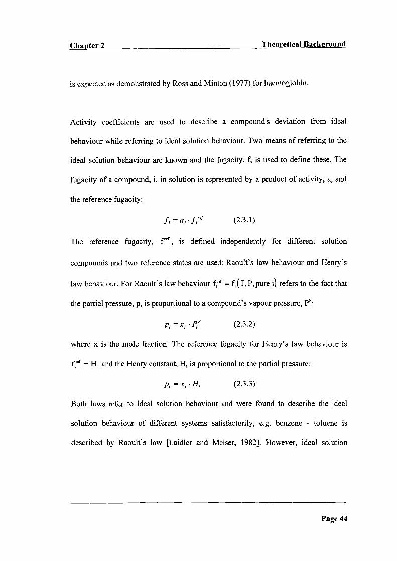
Activity coefficients are used to describe a compound's deviation from ideal
behaviour while referring to ideal solution behaviour. Two means of referring to the
ideal solution behaviour are known and the fugacity, f, is used to define these. The
fligacity of a compound, i, in solution is represented by a product of activity, a, and
the reference fugacity:
(2.3.1)
The reference fugacity, f', is defined independently for different solution
compounds and two reference states are used: Raoult's law behaviour and Henry's
law behaviour. For Raoult's law behaviour = f (T, P, pure i) refers to the fact that
the partial pressure, p. is proportional to a compound's vapour pressure, pS:
(2.3.2)
where x is the mole fraction. The reference fugacity for Henry's law behaviour is
f ref = H 1 and the Henry constant, H, is proportional to the partial pressure:
p1 =x1 . H1 (2.3.3)
Both laws refer to ideal solution behaviour and were found to describe the ideal
solution behaviour of different systems satisfactorily, e.g. benzene - toluene is
described by Raoult's law [Laidler and Meiser, 1982]. However, ideal solution
Page 44

Chapter 2 Theoretical Background
behaviour is only observed for mixtures of similar compounds, which are of the same
molecular size and exhibit the same interactions. Other systems exhibit deviation
from ideal solution behaviour, which has to be accounted for with reference to ideal
behaviour.
For a compound for which the standard state is the pure liquid, the activity, a, in the
standard state is equal to unity. In these cases the standard fugacity, fD, is equal to:
Jo fref pS (2.3.4-5)
It follows for the chemical potential, .t, that:
u,(T,P)=,u,°(T,P)+R• T . ln(a,) (2.3.6)
where a —+ 1 and .t —+ as x —+ 1 which refers to Raoult's law and introduces the
symmetric reference system. For Henry's law a hypothetical standard state is created
where the compound's activity is equal to one in pure solvent, which introduces the
unsymmetric reference state with a 1 —+ 1 as x 1 —* 0.
The activity is defined as the product of a compound's concentration and activity
coefficient, y. Different concentration scales lead to different activity and activity
coefficient expressions:
Page 45

Chapter 2 Theoretical Back2round
a =x. 'Y ()u(x) I
a. =m 7i(m) (2.3.7-9)(rn) I
aI(C) =Cj Yi(c)
where x is the mole fraction, m the molal and c the molar concentration scale.
Deviations from ideal solution behaviour are described by the activity coefficients,
which are a function of the specified standard state and the concentration scale. The
activity coefficients are denoted differently with respect to the standard state chosen.
For Henry's law behaviour, i.e., the unsymmetric convention, a special notation is
made: *• Otherwise Raoult's law behaviour, i.e., the symmetric convention, is
applied. The explicit activity coefficient expressions studied in this work are
introduced in the following chapters and the symmetric and unsymmetric activity
coefficient equations are presented.
2.4. The Original UNIQUAC Model
The original UNIQUAC model [Abrams and Prausnitz, 1975] links the microscopic
and the macroscopic solution scale, creating a thermodynamic framework to describe
solution activity coefficients of pure or mixture systems over temperature. The three
dimensional arrangements and interactions of molecules as represented by lattice
theory (microscopic level) relate to the excess Gibbs energy (macroscopic level). By
Page 46
Chapter 2 Theoretical Background
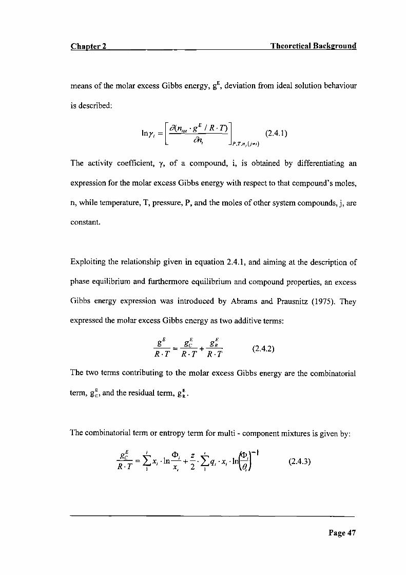
means of the molar excess Gibbs energy, gE, deviation from ideal solution behaviour
is described:
lny, = [(nio1 . gE / R
T)1 (2.4.1)JP,T,nj(j^i)
The activity coefficient, ', of a compound, i, is obtained by differentiating an
expression for the molar excess Gibbs energy with respect to that compound's moles,
n, while temperature, T, pressure, P. and the moles of other system compounds, j, are
constant.
Exploiting the relationship given in equation 2.4.1, and aiming at the description of
phase equilibrium and furthermore equilibrium and compound properties, an excess
Gibbs energy expression was introduced by Abrams and Prausnitz (1975). They
expressed the molar excess Gibbs energy as two additive terms:
gE - g + (2.4.2)R•TR•T R•T
The two terms contributing to the molar excess Gibbs energy are the combinatorial
term, g, and the residual term, g.
The combinatorial term or entropy term for multi - component mixtures is given by:
E jg c1. zR•T
= -' .1n__L+_.q, .xi . 1n) (2.4.3)
Page 47

r..x q.xand e,= 1 ' (2.4.4-5)
Chapter 2 Theoretical Background
where
The combinatorial term accounts for deviation from ideal solution behaviour due to
differences in size and shape of the mixture compounds. The mole fraction, x, refers to
the mixture composition for all compounds, i, while the parameters (J) and 0 represent
the volume and surface fraction of the different compounds, respectively. The structural
parameters r and q refer to the volume and surface area of each compound, i.e.,
molecule, and z indicates the number of nearest neighbours, i.e., the co - ordination
number. The value, z, is generally set equal to 10 but ranges from 6 - 12 representing
the unit cell configuration of the lattice, e.g. z = 6 for the regular cubic lattice and z =
12 for the hexagonal lattice [Tanlord, 1961]. To compute the combinatorial
contribution the structural parameters, r and q, have to be determined for each system
compound. These are derived from a compound's van der Waals volume, V,, and
surface area, A, while being normalised with respect to the methylene molecular
group in polyethylene, which was an arbitrary choice by Abrams and Prausnitz
(1975):
r = 1517
(2.4.6)
Aq
= 25l0(2.4.7)
Page 48

Chapter 2 Theoretical Background
To obtain a compound's van der Waals volume and surface area the group
contribution method by Bondi (1968) is generally applied. However, depending on
the compound Bondi's method might not be adequate and ways to obtain this data for
proteins were developed. These are described when relevant.
The residual term or enthalpy term is given by:
g (j
R=_q,.x,.lnIoJ .vfJI J (2.4.8)
"I
( [u..—u..1= exp— [
T(2.4.9)
With the residual term short - range interactions of a centre molecule with its ten (z)
surrounding next neighbours are introduced using binary interaction parameters, u.
Interaction parameters describe the sum of interactions between a nearest neighbour
and a centre molecule over the various binary interactions occurring per compound
pair. The interactions between identical and different molecule pairs are described by
a number of binary interaction parameters. Three interaction parameters describe for
two compounds, i and j, the binary interactions between identical, u 1 and u, and
different, u with u = ui,, compound types. The total number of binary interaction
parameters, b, needed per system is a function of the number of system compounds, i,
and is given by:
Page 49

Chapter 2 Theoretical Background
b = (i) + (i - l)+...+(i - i) (2.4.10)
These interaction parameters are available from previous modelling attempts for some
compounds. However, they are a function of the studied model version and might
therefore not apply. Following these facts the interaction parameters have to be
established for some compounds and this was the case for this work as proteins had not
been studied before. A programming procedure was designed and FORTRAN
programs were developed during the course of this work in order to obtain these
parameters. These procedures are explained where relevant, while the programs are
printed in the appendices.
Partial molar differentiation of the given g' expressions leads to the activity
coefficient, y, for a compound, i, over the two possible reference states, the
symmetric and unsymmetric reference states:
lny 1 =lnyf+lny,' (2.4.11)
lny,* = lnr*,c + lnr* R (2.4.12)
where is the combinatorial and yR is the residual activity coefficient. In table 2.4.1
the resulting expressions are given with respect to the two terms, combinatorial and
residual term, and the two reference states, symmetric and unsymmetric conventions.
The unsymmetric activity coefficient, y, is obtained from the symmetric activity
coefficient, y, using:
Page 50

Chapter 2 Theoretical Background
Table 2.4.1: The combinatorial term and residual term expressions for activity
coefficient calculations using the original UNIQUAC model
Combinatorial term:
1ny14' = lnJ +1— - • q. [in-) +1-
Sc('\ Cj. r r.
in y,' = in' L _! in +x 1 ) - x 1 - r 01 ) rsoi
- q• [ln-'-J - - 1n" q0j \ +
q01• 1r 0, . q 1 ) r 0, • q1j
Residual term:
1ny1'=q1• 1_lflf Ok WkiJ -°k VIk 1
JWJk
1 [ _________
(k k
Jjmy 1 ' = q [_ ifll ki - + lnsoI.,i +i.I.1"I
Soi.: solvent
Page 51
Chapter 2 Theoretical Background
(2.4.13)V
where y defines the infinite dilution activity coefficient of a compound in pure
solvent.
2.5 The Original UNIFAC Model
Different group contribution models have been developed [Lydersen, 1955; Hoshino
et aL, 1982; Klincewicz and Reid, 1984; Mavrovouniotis et al., 1988; Mavrovouniotis,
1990; Elbro et al., 1991; Constantinou and Gani, 1994] and demonstrated that
compound properties relate not only to the molecule type but also to the molecular
groups, which build a molecule. A great variety of compounds, mainly hydrocarbons
[Lyman et aL, 1982; Reid et a!., 1987], were represented by a limited number of
molecular groups and these were successfiully correlated to a compound's molecular
structure and properties, either pure or mixture properties. These model types, group
contribution models, are able to describe properties not only of previously modelled
compounds or systems but also new and unexamined systems as the molecular
groups allow the creation of any kind of compound and therefore system. This makes
these types of models more widely applicable than other model types. However,
Page 52

Chapter 2 Theoretical Background
extensive and good experimental data over various conditions and systems has to be
available to develop satisfactory group contribution models, which should make the
models applicable for systems and system conditions related to the originally used
systems, i.e., systems of the database used to train the model and to obtain the needed
parameters.
Fredenslund et al. (1975) integrated such a group contribution concept into the
previously presented UNIQUAC model, chapter 2.4, and created the UNTFAC model.
The group contribution approach of the UNIFAC model uses also molecular groups,
which combine to build a compound and lead to that compound's properties using the
properties of the molecular groups that build that compound. For calculations with the
UNIFAC model, as in the case of the UNIQUAC model, the structural parameters, r
and q, of a compound, i, are needed. In the case of the UNILFAC model these are
obtained from the structural parameters, R and Q, of the defmed molecular groups, p,
as a function of their occurrence, v, in that same compound:
(2.5.1)
q=v . Q (2.5.2)
Two sets of structural parameters are introduced. One for the compound, r and q, and
one set for the molecular groups, R and Q . Both sets of structural parameters relate to
Page 53
P®.tIJqipq)_ _/ P
I o,tIIqp(2.5.4)
Chapter 2 Theoretical Background
the van der Waals volume and surface area of either a compound or a molecular group
as discussed before. By means of these molecular groups and their parameters the
group contribution approach was introduced into the UNIFAC model. For the
combinatorial term of the UNIFAC model the same equations apply as for the
UNIQUAC model, equations 2.4.3 - 2.4.5, and the same theory applies as described
before, chapter 2.4.
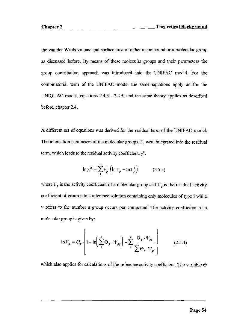
A different set of equations was derived for the residual term of the UNIFAC model.
The interaction parameters of the molecular groups, F, were integrated into the residual
term, which leads to the residual activity coefficient, y':
lny1R =v;.(lnr'-1nr';) (2.5.3)
where [ is the activity coefficient of a molecular group and F 1, is the residual activity
coefficient of group p in a reference solution containing only molecules of type i while
v refers to the number a group occurs per compound. The activity coefficient of a
molecular group is given by:
lnF =QP{1_1n(®P
which also applies for calculations of the reference activity coefficient. The variable 0
Page 54
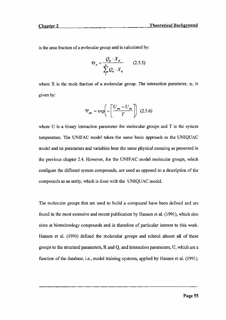
Chapter 2 Theoretical Background
is the area fraction of a molecular group and is calculated by:
®p= qQP•XP(2.5.5)
Qq•Xq
where X is the mole fraction of a molecular group. The interaction parameter, w is
given by:
'pq exp[
[Upq_Uqq
Tj) (2.5.6)
where U is a binary interaction parameter for molecular groups and T is the system
temperature. The UNIFAC model takes the same basic approach as the UNIQUAC
model and its parameters and variables bear the same physical meaning as presented in
the previous chapter 2.4. However, for the UNIFAC model molecular groups, which
configure the different system compounds, are used as opposed to a description of the
compounds as an entity, which is done with the UNIQUAC model.
The molecular groups that are used to build a compound have been defmed and are
found in the most extensive and recent publication by Hansen et al. (1991), which also
aims at biotechnology compounds and is therefore of particular interest to this work.
Hansen et a!. (1991) defmed the molecular groups and related almost all of these
groups to the structural parameters, R and Q, and interaction parameters, U, which are a
function of the database, i.e., model training systems, applied by Hansen et al. (1991).
Page 55

Chapter 2 Theoretical Background
However, reconstruction of a system's compounds using the defined molecular groups
allows for activity coefficient predictions applying the determined parameters and
introduced UNIFAC equations.
2.6 The Modified Model
In 1987 a modified model [Larsen Ct al., 19871 was developed. The combinatorial term
was changed compared to the original one and was since widely used for polymers
[Kontogeorgis et a!., 1997, and references within]. Additionally, a temperature
dependence was introduced by Larsen et a!. (1987) for the residual term and its
interaction parameters. These alterations improved excess enthalpy estimations from
deviation of around 50 % to around 10 % [Fredenslund, 1989]. Consequently,
modelling of systems that span a certain temperature range can be improved using the
modified residual term. Therefore, the modified residual term was studied for this work
when temperature ranges of up to 30 K had to be described for protein solubility.
For the modified model the combinatorial activity coefficients, y, of a compound, i, is
described by:
Page 56

Chapter 2 Theoretical Background
inr,c 1J
(0.= - +1__i(2.6.1)
xi
where
2
x •r,3
= j 2 (2.6.2)
x .rJ
The modified combinatorial term is a function of the volume fraction, co, and the mole
fraction, x, and resembles closely the original combinatorial term, equation 2.4.3 and
table 2.4.1. However, the second part of the original combinatorial term is eliminated.
Due to this the entropy state of solution is described only by means of compound sizes
and reflects the originally suggested expression of Flory - Huggins [Larsen et al.,
1987].
The volume fraction of the modified model, equation 2.6.2, is determined from the
mole fractions of compounds, i and j, and relates closely to the definition given for the
original model, equation 2.4.4. However, the volume parameter, r, was assigned a
smaller contribution as examined and discussed by Kikic et a!. (1980). The introduced
exponent, which is generally and for this work set equal to 2/3, lowers the volume
contribution. The value of the exponent might vary with the type of molecule. The
structural volume parameter, r, is obtained in the manner described before, equations
2.4.6 or 2.5.1, and represents a compound's van der Waals volume as discussed before.
Page 57

Chapter 2 Theoretical Background
The residual term of the modified model is derived in the same manner as for the
original model, chapter 2.4, but a higher order temperature dependence is added for the
binary interaction parameters, u. This results in up to three parameters per binary
interaction parameter instead of one when compared to the original model:
u = u; +u . (T_7')+u .(T.1n-+T_7) (2.6.3)
However, in this work the temperature, T, dependence was terminated after the second
term in order to introduce as few parameters as necessary into the solubility model. The
temperature, T0, is an arbitrary reference temperature which is fixed to 300 K for this
work.
2.7 Appraisal of the Models
The basic model concepts introduced in this work are those of the UNIFAC and
UNIQUAC models. Both models refer to the same theoretical approach but vary with
the extent of their applicability. The UNIQUAC model allows for predictions over
systems conditions such as temperature and composition. The UNIFAC model
allows additionally for predictions over different but related compounds as a function
of the defined molecular groups.
Page 58
Chapter 2 Theoretical Background
Both models have been applied to study phase equilibria and compound properties.
Pure and mixture compound properties were described for a variety of compounds by
various authors [Abrams and Prausnitz, 1975; Fredenslund et a!., 1975; Prausnitz et
at., 1986; Smith and van Ness, 1987]. The compounds investigated were mainly
hydrocarbons and small organic compounds. These relate to some degree to proteins
as discussed earlier, chapter 2.2, and therefore these models were approached.
However, some limitations are indicated for the original models as presented in 1975.
Compounds that bear an electrolyte character just like proteins, which are
polyelectrolytes, were not considered. Likewise, macromolecules such as polymers
and proteins were not included in the early examinations. However, attempts were
made to overcome these limitations and since then polymers and simple electrolytes
were studied with these local composition models while this work is the first
dedicated to proteins.
For polymers it was found that a description of the entropy state of solution alone is
pursued as hardly any interactions are encountered for polymer mixtures built from
aliphatic polymers. Ways to express the entropy state of solution for polymer
mixtures were pursued using the Flory - Huggins combinatorial term as introduced
with the modified model in the previous chapter. While the original combinatorial
Page 59

Chapter 2 Theoretical Background
term bears also the Flory - Huggins expression, it also carries a Staverman -
Guggenheim correction, which in most cases is often quite small [Larsen et al.,
1987]. For the modelling of polymer properties also variations for the definition of
the volume fraction are noted [Couthinho et al., 1994] and differences in the
definition of the volume term and the magnitude of its contribution are introduced.
These works are of relevance for protein containing systems due to the fact that they
have the macromolecular character in common with polymers. Consequently, they
encouraged the study of the original models and their consecutive versions for
proteins. However, the original model and its entropy term were addressed first as
this term already introduces the size impact of the different compounds into the
model as discussed before. While for polymer solutions athermal behaviour is
expected the same cannot be assumed for proteins. Having examined the
characteristics of proteins in chapter 2.2, it is for certain that interactions occur
between proteins and other system compounds. Therefore, the enthalpy state of
solution needs to be described for protein containing systems as done in this work.
Referring to the fact that proteins are polyelectrolytes, studies pursued for simple
electrolytes were of interest. Various research works have been pursued to deal with
electrolyte systems for the UNTQUAC and UNIFAC models since 1986 [Sander et
al., 1986, Nicolaisen, 1994]. To represent the long - range interactions that occur
Page 60

chapter 2 Theoretical Background
between charged groups the Debye HUckel law [Debye and I-IUckel, 1923; Huckel,
1925, Debye, 1927] was introduced. Interactions between charged groups are
observed at low ionic strength in electrolyte solutions. However, high ionic strength
solutions do not encounter charge - charge forces as these are screened off. Dealing
with protein systems that additionally constitute of buffer and salt ions, high ionic
strengths are observed and a screening of the ionic long range interactions is noted
[Kuebner et a!., 1996]. Therefore, this approach was not adapted for the studied
systems and only short - range forces such as dispersion and dipole forces were
accounted for.
Furthermore, it was of interest for this work that recently a new database of
molecular groups and their parameters [Hansen et al., 19911 was published for the
UNIFAC model, which was documented to have been extended to compounds
relevant in biotechnology applications. Success of these parameters for the prediction
of protein activity coefficients or those of related compounds is certainly of interest
for this work. The determination of parameters for the target systems would not be
required, which is a work intensive process depending on the number of parameters
that need to be determined. For the establishment of e.g. a solubility model about
twenty parameters were determined by Nicolaisen (1994) for a system of five
compounds. However, following the fact that a new database, which considered also
Page 61

Chapter 2 Theoretical Background
biotechnology compounds, was introduced for the predictive UNIFAC model
encouraged the use of the discussed modelling frameworks for biotechnology
compounds: proteins.
Consequently, first the UNIFAC model and the new database was examined. The
approaches and results of that work are discussed in the next chapter, chapter three.
This work is then followed by two further result sections which deal with additional
model approach examinations for proteins and lead to the modelling of protein
solubility.
2.8 Summary
The characteristics of proteins, major definitions and models for this work were
introduced and discussed. However, this introduction was limited to the theory
needed throughout this work and for the next chapter, chapter three. Further
definitions and models are introduced when relevant.
Page 62

a
A
b
C
Da
fEg
gE
EgR
H
m
n
p
P
PT
plcpS
q
Q
R
r
R
R
Chapter 2 Theoretical Background
2.9 Nomenclature
activity
Van der Waals surface area
total number of binary interaction parameters
molar concentration
dalton [g!molJ
fugacity
combinatorial term of the molar excess Gibbs energy
molar excess Gibbs energy
residual term of the molar excess Gibbs energy
Henry's constant
compound
molal concentration
number of moles
partial pressure
pressure
isoelectric point
dissociation constant on the pH scale
vapour pressure
structural surface area parameter of a compound
structural surface area parameter of a group
gas constant
structural volume parameter of a compound
structural volume parameter of a group
amino acid residue
Page 63

Chapter 2 Theoretical Background
T temperature
u UNIQUAC binary interaction parameters of a compound
U UNIQUAC binary interaction parameters of a group
UNIFAC model UNIQUAC Functional Activity Coefficients model
UNIQUAC model UNIversal QUAsi Chemical model
V Van der Waals volume
x compound mole fraction
X group mole fraction
z lattice co - ordination number
Greek letters
1'
0
'-I'
7
Il
V
0
(0
'4'
Subscript
0
c
J
volume fraction (org.)
group activity coefficient
group area fraction
group interaction parameter
compound activity coefficient
chemical potential
molecular group occurrence per compound
compound area fraction
volume fraction (mod.)
molecule interaction parameter
standard
molar concentration
compound
compound
Page 64

Chapter 2 Theoretical Background
k compound
molecular group
m molal concentration
p molecular group
q molecular group
tot total
x mole fraction
Superscript
J) infinite dilution
standard
* unsymmetric convention
C combinatorial term
i compound
R residual term
ref reference
t' temperature (third term)
t temperature
Page 65

Chapter 3 Calculation of Amino Acid and Peptide Activity Coefficients
Chapter 3
Calculation of Amino Acid and Peptide Activity Coefficients
It was the objective of this part to evaluate which model approach describes a
solution and mixture property, activity coefficients, of amino acids and peptides.
3.1 Introduction
Aiming at the description of protein solubility by means of protein activity
coefficients required first the examination of the various activity coefficient models.
The UNIFAC [Fredenslund et a!., 1975] and UNIQUAC [Abrams and Prausnitz,
1975] models and their consecutive versions were investigated for their ability to
describe activity coefficients using binary systems of amino acids arid peptides in
water. These compounds were chosen as they are the building blocks of proteins, the
Page 66

Chapter 3 Calculation of Amino Acid and Pe ptide Activity Coefficients
target compounds, and it is hypothesised that models perfonning for these
compounds will also perform for proteins due to their molecular similarities.
Furthermore, activity coefficient data is available for these systems but not for
proteins.
A systematic study of the various model versions was adopted with the aim to
establish, which model type is applicable for amino acids and peptides and therefore
most likely also for proteins. However, a model that performs for amino acid and
peptide activity coefficient calculations would need to be examined for proteins next
as molecular size differences of these compound classes are significantly different.
The UNIFAC group definitions, the group parameters, the model approaches and
activity coefficient reference states were investigated for amino acids and peptides.
Furthermore, for the first time the original UNIFAC model [Fredenslund et al., 1975]
with the established molecular groups and parameters of Hansen et al. (1991) was
studied. This was of particular interest for this work as biotechnology compounds
had been considered by Hansen et al. (1991) making the model likely to succeed for
proteins and related compounds, i.e., amino acids and peptides. While first of all the
UNIFAC model was approached because of its predictive properties, an examination
of the UNIQUAC model was also pursued.
Page 67

Chapter 3 Calculation of Amino Acid and Peptide Activity Coefficients
3.2 Activity Coefficient Data
Activity coefficient data of six aqueous amino acid and three aqueous peptide
systems at 25 °C was obtained [Edsall and Wyman, 1958]. Hence, the activity
coefficient data of nine different compounds was examined in this work: glycine,
alanine, valine, serine, threonine, proline, glycyiglycine, glycylalanine and triglycine.
These compounds reflect the different properties that are found for the different
residues of amino acids, peptides or proteins, chapter 2.2. The first three compounds
represent non - polar characteristics while the next two, serine and threonine, are
polar. The imino acid proline represents a steric hindered residue and the three small
peptides refer to a protein's peptide bonding and backbone formation.
The data for these nine systems had to be converted into the thermodynamic
concentration scale: mole fractions and activity coefficients referring to the mole
fraction scale. To convert the data from the molal scale the following equations were
applied [Soehnel and Garside, 1992; Nicolaisen, 1994]:
xi' (3.2.1)
mj . 'Snlvent + 1
Yi(x) r,(m)
j= . . 1+ I (3.2.2)
1)
Page 68

Chapter 3 Calculation of Amino Acid and Peptide Activity Coefficients
The mole fraction, x, of compound, i, is obtained from the molal concentration, m, of
that compound, the solvent's molecular weight, M, and the molal concentrations of
further compounds, j. The activity coefficient on the mole fraction scale, y,, is
calculated from the molal activity coefficient, y, the solvent's molecular weight and
the molal concentrations of further system compounds.
In cases where the data is provided on the molar scale the following conversions
were applied:
C 'SoIvenix. = J (3.2.3)
Psotusion + (Moj,,ng - M')
j
Poiui ion + (Movg - M) 1Yi(x) Yi(c) I (3.2.4)
Poiven,
J
To obtain a compound's mole fraction and activity coefficient on the mole fraction
scale the molar concentrations, c, of all compounds, i and j, are needed. Additionally,
the solvent's molecular weight and compounds' molecular weights have to be known
while also the solution and solvent density, p, are necessary for the calculations. As
the solution density was not available for the mixture systems studied the solvent
density, i.e., water density, was applied. This was justified following the fact that
water is the main compound of the systems where the second compound, either an
Page 69

Chapter 3 Calculation of Amino Acid and Peptide Activity Coefficients
amino acid or a peptide, occurs at low concentrations, appendix A. Conversions into
the thermodynamic scale, x and ',, were pursued as part of this work and the
obtained data of all nine systems, which were studied here, is given in appendix A.
3.3 Study of the UNIFAC and UNIQUAC Models
The activity coefficient data of nine amino acids and peptides, which build a binary
system with water as the solvent, was modelled using the UNIFAC and UNIQUAC
models. The models used in this chapter were introduced in detail in the previous
chapter, chapter two, and the programs to pursue these investigations were obtained
from different sources.
Routines for all IINIFAC models using the symmetric convention were supplied by
Prof. R. Gani from the Chemical Engineering Department at the Technical University
of Denmark, Lyngby. To use these models slight modifications were added to the
programs as part of this work. This made the programs applicable for the systems,
i.e., amino acids and peptides, studied here. A routine for the UNIFAC model based
on the unsymmetric convention was made available by Prof. F.L.P. Pessoa from the
Chemical Engineering Department of the Federal University of Rio de Janeiro in
Page 70

Chapter 3 Calculation of Amino Acid and Peptide Activity Coefficients
Brazil. The programming routine for the UNIQUAC model used here was designed
and programmed as part of this work and is documented in appendix B.
3.3.1 Study of the UNIFAC Model
In order to apply the UINIFAC model [Fredenslund et al., 1975] the molecular
structures of all system compounds were examined and the molecular groups
required to assemble the compounds according to Hansen et a!. (1991) definitions
were determined. In table 3.3.1.1 the structures of the nine compounds [Lehninger,
1982] and the defined UNIFAC molecular groups, i.e., UNIFAC groups [Hansen et
a!., 1991], are given. Up to five different UNIFAC groups are used for a molecule
e.g. threonine. For one case, glycylalanine, the CONHCH group is not available and
was therefore substituted by the structurally related CONHCH 2 group. This
substitution will be discussed when reviewing the results as further approaches of
this kind were pursued. For these groups, table 3.3.1.1, parameters and binary
interaction parameters as given by Hansen et a!. (1991) were applied for the model
calculations unless stated differently. For water, the second system compound, the
established groups and parameters were applied [Abrams and Prausnitz, 19751.
Page 71

Proline CH2-NH
ClT!2 I
CH2-C(H)-C(=O)(OH)
Alanine
H2N-.CH(CH3)-C(=O)(OH)
Valine
H2N-CH(CH(CH3)2)-C(=O)(OH)
Serine
H2N-CH(CH2OH)-C(=O)(OH)
Threonine
H2N-CH(CH(OH)(CH3))-C(=O)(OH)
H2NCH, COOH, CH2,
OH
H2NCH, COOH, CII,
CH3 , OH
INCH, COOH, 3 CH
H2NCH, COOH, 2 CH3,
CH
H2NCH, COOH, Cl3
Chapter 3 Calculation of Amino Acid and Peptide Activity Coefficients
Table 3.3.1.1: Molecular structures of amino acids and peptides and their UNIFAC
groups
Compound Molecule structure UNIFAC groups
Glycine H2N-CH(H)-C(0)(OH) H2NCH2, COOH
Glycyiglycine H2N-CH(H)-C(0)NH-CH(H)-C(0)(OH) H2NCH2, COOH,
CONHCH2
Glycylalanine H2N-CH(H)-C(0)NH-CH(CH 3)-C(0)(OH) H2NCH2, COOH,
CONHCH2, CH3
Triglycine H2NCH(HC(0)NH..CH(HC(0)NH-CH(H)-C(0)(OH) H2NCH2, COOH,
2 CONHCH2
Page 72

Chapter 3 Calculation of Amino Acid and Peptide Activity Coefficients
In table 3.3.1.2 the results for the calculations for the nine systems are listed. Four
different sets of calcuLations were pursued with the UNIFAC model studying the
group definitions, group parameters, model versions and activity coefficient
reference states. The model performances for these calculations are given in table
3.3.1.2 referring to the root mean square deviation, rmsd. The root mean square
deviation describes the error between modelled data, cal., and experimentally
determined data, exp., over all data points, N. The root mean square deviation is
evaluated using the standard square deviation, ssd:
ssd=1 (3.3.1.1)exp. )
and
rmsd l00%.(-.ssd) (3.3.1.2)
The root mean square deviation is computed as a percentage and a low percentage
indicates a good model performance, where a root mean square deviation of 0 % is
the best achievable model performance. All model evaluations of this work were
scaled and judged using the root mean square deviation.
For this part of the work four consecutive sets of calculations were pursued. The
results of these are presented next. Following this, the results of the four different
calculations are reviewed together. Moreover the work of Pinho et al. (1994) was
Page 73

Chapter 3 Calculation of Amino Acid and Peptide Activity Coefficients
Table 3.3.1.2: Performance of the activity coefficient calculations for amino acids
and peptides using various UNIFAC model versions
case compounds model type rmsd [%]
1 Glycine original UNIFAC (symmetric) 73
2 Alanine original UNIFAC (symmetric) 11
3 Valine original UNIFAC (symmetric) 377
4 Serine original UNIFAC (symmetric) 14
5 Threonine original UNIFAC (symmetric) 53
6 Proline original UNIFAC (symmetric)
7 Glycylglycine original UNIFAC (symmetric) 95
8 Glycylalanine original UNIFAC (symmetric) 92
9 Triglycine original LJNIFAC (symmetric) 99
10 Glycine original UNIFAC (symmetric) and altered groups 69
11 Valine original UNIFAC (symmetric) and altered groups 882
12 Threonine original UNIFAC (symmetric) and altered groups 53
13 Pro line original UNIFAC (symmetric) and altered groups
14 Glycine modified IJNIFAC (symmetric) 60
15 Valine modified UNIFAC (symmetric) 113
16 Threonine modified UNIFAC (symmetric) 44
17 Proline modified UNIFAC (symmetric) 124
18 Glycine original UNIFAC (unsymmetric) 49
19 Pro line original UNIFAC (unsymmetric)
Page 74

Chapter 3 Calculation of Amino Acid and Peptide Activity Coefficients
integrated into this review as they had investigated yet another UNIFAC model
version. They had defined amino acid and peptide specific groups and determined
their parameters, which led to activity coefficient predictions. Their results and those
from this work will be discussed and used to direct this work further.
The first set of calculations, table 3.3.1.2, pursued as part of this work used the
original UNIFAC model on the symmetric scale to compute activity coefficients for
all nine systems (cases 1 - 9). The model gave deviations from 11 - 395 % for the
nine systems. The poor performance of the original UNIFAC model on the
symmetric scale using the parameters of Hansen et al. (1991) was thought to be
mainly due to the fact that some interaction parameters were missing for the defined
groups. For the H2NCH2 and H2NCH groups binary interaction parameters with the
COOH group are listed by Hansen et al. (1991) as zero. This implies that the sum of
interactions occurring between the molecular groups is zero, which is not necessarily
true for these groups. If they are in the vicinity of each other interactions are likely to
occur due to their dipole moments, chapter 2.2. Therefore these interaction
parameters might have led to the unsatisfactory results. Following this hypothesis a
second set of calculations was pursued using structurally related groups with
interaction parameters.
Page 75

Chapter 3 Calculation of Amino Acid and Peptide Activity Coefficients
For the second set of calculations (cases 10 - 13), table 3.3.1.2, the lack of interaction
parameters was overcome by introduction of different UNIFAC groups. Groups,
which have interaction parameters listed, and relate most closely in their molecular
structure to the ones used for the first calculations were used. This approach was
taken as it had been demonstrated by Fredenslund et at. (1975) and Hansen et al.
(1991) that similar molecular structures such as CH, CH 2 and Cl3 bear the same
property contribution and therefore were assigned into one group, main group, of
same interaction parameters. Furthermore, it can be assumed that similar molecular
structures have similar interactions occurring. However, this is only true for some
relating molecular structures but not all, as manifested in the group contribution
method where a set of different molecular groups is created. Still, the groups that
missed interaction parameters, H 2NCH2 H2NCH and COOH, were substituted with
the CH2NH, CHNH and COO main groups, respectively. Following this, four
selected systems, glycine, valine, threonine and proline, were studied with altered
groups. These systems were selected as they showed the lowest and highest
deviations in the previous calculations and because they demonstrate different
activity coefficient behaviour, i.e., negative and positive deviation from ideal
behaviour. Furthermore, they represent the different residue characteristics as
discussed in chapter 2.2. Following the hypothesis that the assumed interaction
parameters of zero caused the poor results for the original UNIFAC model (cases 1 -
Page 76

Chapter 3 Calculation of Amino Acid and Peptide Activity Coefficients
9) the same model type was applied but altered groups, i.e., CH 2NH, CHNH and
COO, with their interaction parameters were used. However, no improvement was
found for these calculations. For the same model type with a different set of groups
the deviations almost doubled when compared to the first calculations. A doubling of
the deviation was observed in two cases: valine (case 11 and 3) and proline (case 13
and 6). This result was interpreted as a possible deficiency in the model. Therefore,
the original UNIFAC model was substituted with a different model approach, the
modified UNIFAC model, to examine this hypothesis.
For the third set of calculations, table 3.3.1.2, the modified model (cases 14 - 17) was
studied. The symmetric scale was used and the same set of four systems was studied
while the first set of group definitions was applied. For the systems previously
performing most poorly, valine and proline, better results were obtained and an
improvement by a factor of three is observed compared to the first calculations (cases
3 and 6). Still, deviations of around 100 % were obtained which is not satisfactory.
Qualitative examination of the calculated activity coefficients and those from
experiment demonstrates also that no improvement was made. The qualitative
behaviour of experimentally determined and modelled activity coefficients shows no
correlation. At this point of the work it was unclear what caused the high deviations:
the group definitions, their parameters or the model approach. Neither a change of
Page 77

Chapter 3 Calculation of Amino Acid and Peptide Activit y Coefficients
the group definitions and parameters nor a change of the model version showed
improvement. However, the activity coefficient reference state had not yet been
examined. Therefore, the unsymmetric reference state was examined for its impact
on the activity coefficient description.
The fourth and last set of calculations, table 3.3.1.2, examined the original UNIFAC
model using the unsymmetric scale for the glycine and proline systems (cases 18 -
19). The results of these calculations and the model approach used are directly
comparable to the first calculations (cases I and 6) as only the applied reference state
differs. The unsymmetric scale has a major impact on the model performance.
Deviations of modelled and experimentally determined activity coefficients are the
lowest so far obtained. For proline a deviation of only 36 % and for glycine a
deviation of only 49 % resulted. Noticeable improvement was made by introduction
of the unsymmetric scale but still no improvement for the qualitative behaviour is
found. Figure 3.3.1.1. demonstrates that the model calculates the opposite behaviour
to the behaviour determined from experiment. However, the fact that the
unsymmetric scale reduces the deviation of pro line by a factor of ten when compared
to the symmetric scale leads to the conclusion that amino acids and related
compounds, i.e., proteins, follow Henry's law for reference purposes. This was also
found by Fraaije et al. (1991) from adsorption experiments with proteins, which are
Page 78

1.7du1e
1.5
'-i 13
I1.1
c)
0
ycine
0.7
0.5
0.00 0.01 0.02 0.03 0 04 0.05 0.06
Chapter 3 Calculation of Amino Acid and Peptide Activity Coefficients
jgure 3.3.1.1: Experimentally determined and modelled (original UNIFAC
unsymmetric) activity coefficients of glycine and proline against the amino acid and
peptide mole fraction
Mole fraction [-}
Symbols represent experimentally determined data. Lines represent model calculations.
Page 79

Chapter 3 Calculation of Amino Acid and Peptide Activity Coefficients
the target compounds of this work and relate to amino acids and peptides. As a result
of this work the unsymmetric standard state was applied for the activity coefficient
calculations in the following parts.
The results from the four calculation sets demonstrate that the UNIFAC model is not
applicable in its present state for the compounds examined. A combination of causes
might be responsible for the poor performances. However, the model failure is
thought to be mainly due to the fact that the compounds were not fully represented.
Model parameters and group definitions seem inappropriate. For glycylalanine the
group representing the peptide bond of the molecule is missing. This documents that
the UNIFAC group definitions are not appropriate for proteins as the peptide bond is
an important molecular group for all proteins. The peptide bond builds a protein's
backbone as discussed in chapter 2.2. Additionally, binary interactions of so far three
molecular groups are not available. The interactions of the amino terminus with the
carboxyl terminus and the carboxyl group of the acidic residues (aspartic acid,
glutamic acid) are not described. The missing interactions and the non existence of a
peptide group show that similar compounds were not used to establish the model
parameters, which most possibly leads to the unsatisfactory quantitative and
qualitative performance. However this does not yet invalidate the model as only
incorrect group definitions and parameters are possibly responsible for the bad model
Page 80

Chapter 3 Calculation of Amino Acid and Peptide Activity Coefficients
performances. Additionally, confirmation of the unsymmetric reference scale by
means of these IJNIFAC model studies allows for the assumption that the modelling
base is satisfactory for the studied compounds. However, this is further questioned
and discussed next.
The UNIFAC model might perform satisfactorily for the systems of interest
hypothesising that the model approach is appropriate. Introduction of the systems
into the database, which is used to establish the model parameters should improve the
model performance. Pinho et al. (1994) have demonstrated that indeed the UNIFAC
model performs better when the model parameters are established from a database
that contains amino acids and peptides. They computed activity coefficients with
their newly established model parameters and found average deviations of about 0.5
% with a maximum of 1.2 % for proline. Their results implied that the modelling
base is appropriate.
However, predictions pursued by Pinho et al. (1994) for related but new systems, that
were not previously included in the database used to obtain the model parameters,
showed maximum deviations of 17 % (glyclglycine) or even 28 % (glycylalanine)
when compared to the experimentally determined data over composition. This
predictive performance is already better than the one found from the work pursued
Page 81

Chapter 3 Calculation of Amino Acid and Pe ptide Activity Coefficients
here and confirms the impact of the reference database. Still, the performance is not
satisfactory and this is most likely still due to the limitations of the database used to
obtain the model parameters. The database of Pinho et a!. (1994) consisted of only
seven systems and was therefore not fully representative for related but new systems.
Limited experimental data leads to unsatisfactory group contribution methods and is
certainly a matter of concern as only limited experimental property data is available
for the targeted compounds, i.e., proteins. This makes the study of the UNIFAC
model at this stage unrealistic, where as a next step a correlative approach is focused
on as no parameters are available to describe the target compounds. However, the
UNIFAC model in its present state with the group definitions and parameters of
Hansen et a!. (1991) had to be examined for protein related compounds in order to
clarify its applicability as it might have been successful as it is successful for many
other compounds.
Following this, the related UNIQUAC model was examined next as part of this work.
This model allows closer examination of the modelling approach due to the fact that
no group contribution approach is added. This reduces the number of parameters
required for calculations. Furthermore, the amount of experimental data necessary is
reduced while also deviations due to possibly incorrectly defmed UNIFAC groups
are eliminated. However, the predictive ability over related but different compounds
Page 82

Chapter 3 Calculation of Amino Acid and Peptide Activit y Coefficients
is lost.
3.3.2 Study of the UNIQUAC Model
The UNIQUAC model [Abrams and Prausnitz, 1975] evolved from the same
theoretical approach as the UNIFAC model but it represents system compounds
differently. Compounds are represented as molecular entities. Due to this kind of
compound description less model parameters are needed, which elucidates model
calculations and model approach investigations in comparison to the previously
examined IJNIFAC model. Additionally, less experimental data is needed for the
model as less parameters have to be determined and experimental data is limited for
the targeted compounds, i.e., proteins. Aiming predominantly at the establishment of
a model base and following the fact that only limited reference data is available the
original UNIQUAC model was applied here. In any case a correlative approach was
to be examined as a next step as no appropriate parameters are available for the target
compounds. The unsymmetric scale was used following the presented results with
the UNIFAC model, chapter 3.3.1.
Three of the previously studied systems were examined: glycine, proline and
Page 83

Chapter 3 Calculation of Amino Acid and Pe ptide Activity Coefficients
glycylglycine. The first two systems were chosen as they have been examined here
for all the different UNIFAC model types and because they demonstrate different
activity coefficient behaviour over composition. Glycyiglycine was chosen to
examine a peptide containing system.
In order to apply the UNIQUAC model the binary interaction parameters and
structural parameters had to be determined. The structural parameters, r and q, were
obtained from the publication of Peres and Marcedo (1994) and are listed in table
3.3.2.1. The interaction parameters, u, for the three systems had to be obtained
independently. The procedure for the parameter determination is discussed in the
next chapter, chapter four, while the interaction parameters determined as a result of
this work are given in table 3.3.2.1. Per compound pair one interaction parameter was
determined and for each of the binary systems investigated three interaction
parameters resulted. In total seven new parameters were obtained to describe the4
three system ' The results of the model calculations are given in table 3.3.2.2. Use of
the original UNIQUAC model shows much better results when compared to the
UNIFAC model, table 3.3.1.2. With the UNIQUAC model root mean square
deviations of 0.1 - 0.3 % were achieved for the three systems when comparing
modelled and experimentally determined activity coefficient data. Additionally, the
agreement of model calculations and the experimentally determined activity
4or a
4tCo c(kyv\ e4ec- cks wQck
Page 84

Chapter 3 Calculation of Amino Acid and Peptide Activity Coefficients
Table 3.3.2.1: Structural parameters and binary interaction parameters for glycine,
proline, glycyiglycine and water
H20 Glycine Proline Glycyiglycine r q
[K] [K] [K] [K] [-] [-]
H20 78.69 - 264.0 - 302.2 - 269.1
1.40 0.92
Glycine - 801.3
2.67 2.46
Proline - 806.3
4.30 3.46
Glycyiglycine - 806.6 4.65 4.04
Table 3.3.2.2: Performance of the activity coefficient calculations for glycine, proline
and glycyiglycine using the original UNIQUAC model (unsymmetric)
case compounds model rmsd [%]
1 Glycine original IJNIQUAC (unsymmetric) 0.1
2 Proline original UNIQUAC (unsymmetric) 0.2
3 Glycylglycine original UNIQUAC (unsymmetric) 0.3
Page 85

Chapter 3 Calculation of Amino Acid and Peptide Activity Coefficients
Figure 3.3.2.1: Experimentally determined and modelled (original UNIQUAC
unsymmetric) activity coefficients of glycine, proline and glycyiglycine against the
amino acid and peptide mole fraction
1.3
1.2
1.0
1)0C)
0.9>
<0.8
0.7
0.6
0.00
e
0.01 0.02 0.03 0.04 0.05 0.06
Mole fraction [-]
Symbols represent experimentally determined data. Lines represent model calculations.
Page 86

Chapter 3 Calculation of Amino Acid and Peptide Activity Coefficients
Table 3.3.2.1: Eq,crimcntation error evaluation using two sets of experimentally
determined activity coefficient data for glycine, serine and glycyiglycine
x Glycine# Glycine Serine# Serine G1ycy1g1ycine Glycylg1ycine
0.0036 0.9637 0.9644 0.9540 0.9673 0.9145 0.9153
0.0054 0.9531 0.9487 0.9340 0.9492 0.8821 0.8838
0.0089 0.9158 0.9213 0.8951 0.9160 0.8308 0.8354
0.0125 0.9048 0.8981 - - 0.7917 0.8006
0.0177 0.8910 0.8697 - - 0.7154 0.7581
0.0263 0.8410 0.8342 - - 0.7079 0.7155
0.0348 0.8 152 0.8098 - - - -
0.043 1 0.7962 0.7909 - - - -
Error Glycine Serine Glycylglycine
ssd 0.0008 0.0010 0.0038
I-]
rmsd 1.02 1.83 2.53
[%]
#: Sober, 1968; $: Edsall and Wyman, 1958
Page 87

Chapter 3 Calculation of Amino Acid and Peptide Activity Coefficients
coefficient data is shown in figure 3.3.2.1. Qualitative and quantitative agreement
resulted for the three systems when the original IJNIQUAC model on the
unsymmetric scale was applied, which is partly due to the fact that a correlation is
examined. However, the low deviation seems to also confirm the model base.
& be ' .c-Lt .cro- v
To judge the model performance an experimentation error was established, table
3.3.2.3. For glycine, serine and glycyiglycine activity coefficient data at same system
conditions is available from two different laboratories [Edsall and Wyman, 1958;
Sober, 19681. Comparisons of the two data sets gave root mean square deviations of
1.0 %, 1.8 % and 2.5 % for glycine, serine and glycyiglycine, respectively. This
4,QkCLi MI'kindicates an average cxperimcntation error of 1.8 %. These results demonstrate that
the deviations of 0.1 - 0.3 % resulting from the UNIQUAC calculations are well
b.t c4 IIi4,&below the experimentation error, confirming the good model performance. Moreover,
these results imply that the model approach is appropriate for amino acid and peptide
systems and therefore most likely also for protein containing systems. This is
assumed as amino acids and peptides are the molecular building groups of proteins
but the next part of this work shall possibly prove this hypothesis. Therefore the
same model was approached for the calculations of protein activity coefficients.
These studies are presented in the next chapter, chapter four.
4 c e lai.A&e$
Page 88

Chapter 3 Calculation of Amino Acid and Peptide Activity Coefficients
3.4 Summary
A systematic comparison of different models was followed for the first time to
calculate activity coefficients for protein related compounds, amino acids and
peptides. This part of the work was pursued in order to evaluate which model would
represent an appropriate approach for protein containing systems and would
eventually model solution and mixture properties.
Nine amino acid and peptide systems were examined demonstrating that the
UNIFAC models and the established parameters are not applicable. Deviations of
well above 100 % resulted when comparing experimentally determined and
calculated activity coefficients. This is possibly mainly due to missing parameters.
Furthermore, molecular groups were not defined according to the needs of the
examined systems. Molecular structures such as e.g. peptide bonds were not
represented for the studied systems. However, the UNIFAC model calculations
demonstrated that the unsymmetric scale should be applied for the calculations of
amino acid and peptide activity coefficients. This was indicated by an improvement
of the deviations to below 50 %. Further work on the UNIFAC model was not
pursued due to the limited amount of experimental data available. Therefore, the
UNIQUAC model was approached.
Page 89

Chapter 3 Calculation of Amino Acid and Peptide Activity Coefficients
A program of the IJNIQUAC model using the unsymmetric activity coefficient scale
was developed as part of this work and applied for three systems, two amino acids
and one peptide system. The binary interaction parameters for these systems were
determined. Deviations of only 0.1 - 0.3 % occurred for the model when calculated
and experimentally determined activity coefficients were compared over varying
LQ'ic&composition. This result is well below the obtained cxperimcntation error of 1.8 %
and indicates that the UNIQUAC model should be examined for protein containing
systems and their solution and mixture properties.
3.5 Nomenclature
c molar concentration
cal. calculated
exp. experimental
m molal concentration
M molecular weight
N number of data points
q structural area parameter of a compound
r structural volume parameter of a compound
rmsd root mean square deviation
ssd standard square deviation
UNIFAC model UNIQUAC Functional Activity Coefficients model
Page 90

Chapter 3 Calculation of Amino Acid and Peptide Activity Coefficients
UNIQUAC model UNIversal QUAsi Chemical model
x compound mole fraction
Greek letters
compound activity coefficient
p density
Subscript
molar concentration
compound
compound
m molal concentration
x mole fraction
Page 91

Chapter 4 Calculation of Protein Activity Coefficients
Chapter 4
Calculation of Protein Activity Coefficients
The determination of protein activity coefficients from osmotic pressure
measurements and the study of the UNIQUAC model to calculate these protein
activity coefficients is documented.
4.1 Introduction
The first part of this work demonstrated that the original UNIQUAC model on the
unsymmetric scale successfully calculated activity coefficients for two amino acids
and one peptide. As amino acids and peptides are the subunits of proteins it was
hypothesised that the same approach is applicable to model activity coefficients of
Page 92

Chapter 4 Calculation of Protein Activity Coefficients
proteins. This hypothesis was examined and the investigation is documented in this
chapter, chapter four. These results are also presented and discussed elsewhere
[Agena et al., 1996; Agena Ct al., 1997b; Agena et al., 1998b].
In order to examine the UNIQUAC model for its ability to express protein activity
coefficients, activity coefficient data was required. Experimental osmotic pressure
data was used to obtain this data. By means of the virial expansion activity
coefficients as a function of solution composition were determined using
experimental osmotic pressure measurements from various sources. Ten different
systems were examined consisting of four different proteins: serum albumin, a -
chymotrypsin, 3 - lactoglobulin and ovalbumin. The determined activity coefficient
data was used to study the original UNIQUAC model. The protein activity
coefficient behaviour as a function of salt concentration, pH and temperature was
examined to validate the model performance while additionally protein solubility was
investigated.
Page 93

Chapter 4 Calculation of Protein Activity Coefficients
4.2 Activity Coefficient Data
Activity coefficient data is not documented for proteins but osmotic pressure
measurements were utilised here to obtain protein activity coefficient data.
Experimental osmotic pressure data is available from various laboratories at different
system conditions [Cohn and Edsall, 1943; Guntelberg and Lindstrom-Lang, 1949;
Christensen, 1952; Haynes et al., 1992]. Ten systems and a broad spectrum of system
conditions were studied: four globular protein types, about four different salt types,
protein concentrations of up to 63 gIL, varying salt concentrations, temperatures
around 1 °C and 25 °C, and a pH range from 3 - 12. These systems and their
conditions are listed in table 4.2.1. while the four proteins and their characteristics
have been discussed before, chapter 2.2.
For this work the salt and the solvent, i.e., water, were represented as one pseudo
solvent, which is applicable due to the fact that the salt concentration is held
constant, table 4.2.1. The systems were regarded as binary systems of a solute, i.e.,
protein, and a pseudo solvent, PS. The properties of water were assumed for the
pseudo solvents as water is its main compound. To confirm this approach the activity
coefficient behaviour was examined and discussed in the results section and the
results support the concept of the pseudo solvent.
Page 94

Chapter 4 Calculation of Protein Activity Coefficients
Table 4.2.1: Protein systems and system conditions investigated
System Protein Pseudo Protein conc. t pH Salt, Buffer
solvent [g/L] [°CJ [-1
S Serum Albumin PS 1 10- 48 1 7.4 Phosphate
0.0667 M
Cl a - Chymotrypsin PS 2 0.9 - 40 25 3 Potassium Sulphate
0.05 M
C2 a - Chymotrypsin PS 3 0.9 - 40 25 3 Potassium Sulphate
0.15 M
C3 a - Chymotrypsin PS 4 0.9 - 40 25 3 Potassium Sulphate
0.3 M
C4 a - Chymotrypsin PS 5 0.9 - 9 25 5 Potassium Sulphate
0.1 M
CS a - Chymotrypsin PS 6 0.9 - 9 25 12 Potassium Sulphate
0.1 M
C6 a - Chymotrypsin PS 7 0.9 - 9 25 5 Sodium Phosphate
0.1 M
C7 a - Chymotrypsin PS 8 0.9 - 10 25 8.25 Sodium Phosphate
0.1 M
L - Lactoglobulin PS 9 10 - 47 20 n.k. Sodium Chloride
1 molal
0 Ovalbumin PS 10 23 - 63 20 4.85 Sodium Chloride
1 molal
n.k.: not known, conc.: concentration
Page 95
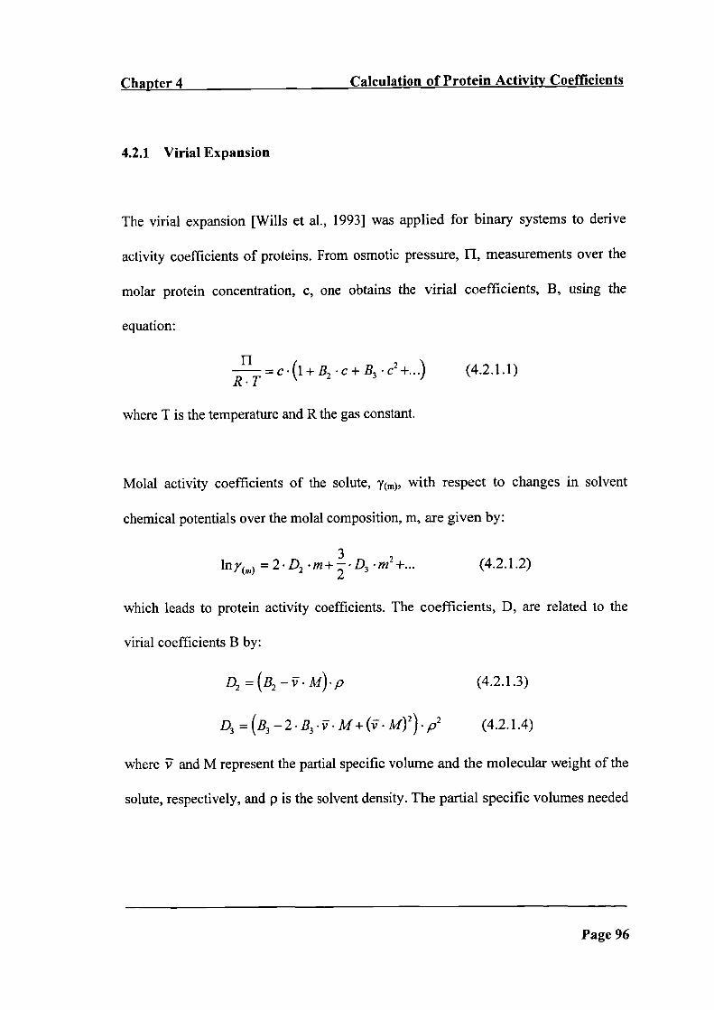
Chapter 4 Calculation of Protein Activity Coefficients
4.2.1 Virial Expansion
The virial expansion [Wills et al., 1993] was applied for binary systems to derive
activity coefficients of proteins. From osmotic pressure, [I, measurements over the
molar protein concentration, c, one obtains the virial coefficients, B, using the
equation:
R.Tc(1+B2c+B3c (4.2.1.1)
where T is the temperature and R the gas constant.
Molal activity coefficients of the solute, 7(m), with respect to changes in solvent
chemical potentials over the molal composition, m, are given by:
3lfly() =2D2 •m+D3 m2 +... (4.2.1.2)
which leads to protein activity coefficients. The coefficients, D, are related to the
virial coefficients B by:
D2 =(B2_ . M) . p (4.2.1.3)
D3=(B3_2.B3.ii.M+(i.M)2).p2 (4.2.1.4)
where 3 and M represent the partial specific volume and the molecular weight of the
solute, respectively, and p is the solvent density. The partial specific volumes needed
Page 96

Chapter 4 Calculation of Protein Activity Coefficients
for the activity coefficient determination were obtained from Sober (1968). The
protein molecular weights originated from the same publications as the osmotic
pressure measurements, chapter 4.2, following the fact that osmotic measurements
are used to obtain the molecular weights of proteins.
The conversion between the molal concentration, m, and molar concentration, c,
scales [Soehnel and Garside, 1992; Nicolaisen, 1994] were computed using:
ci= J
(4.2.1.5)
psolulion - Cf l'Vff
and
m.= (4.2.1.6)C,
1+m .M
The variables are those introduced above while i and j refer to the system
compounds.
To obtain activity coefficient data from osmotic pressure measurements, the reduced
osmotic pressure, fJlc, was scaled over the molar protein concentration, figure
4.2.1.1. Linear or higher order least square fitting was performed as part of this work
in order to determine the virial coefficients, B. For the serum albumin system two
coefficients with values of 0.1771 m 3/mol and 0.5953 (m3/mol)2 resulted. In table
Page 97

Chapter 4 Calculation of Protein Activity Coefficients
4.2.1.1 the B coefficients for all systems are given and a good fitting performance is
Figure 4.2.1.1: Reduced osmotic pressure of the serum albumin system against
protein concentration
1.45
1.40
1.35
1.20
. 1.15C
o 1.10
1.05
1.00
red. pressure! (R T) = 0.5953 c2 + 0.1776c + 1
_____ S _____ _____ _____ _____-. .
.
0 0.1 0.2 0.3 0.4 0.5 0.6 0.7
Molarity [mol!m3J
Symbols represent experimentally determined data. Lines represent model calculations.
Page 98

Chapter 4 Calculation of Protein Activity Coefficients
Table 4.2.1.1: Virial expansion data of protein systems
System Mapparent spec. vol. B2 B3 B4 R2
[g/mol] [cm3/g] [m3/mol] [(m3/mol) 2] [(m3/mol) 3] [_J
S 68598 * 0.748 0.1776 0.5953 - 1.00
Cl 28200 0.736 0.0022 0.0958 - 0.98
C2 26800 0.73 6 - 0.4776 0.2234 - 0.98
C3 27400 0.73 6 - 0.649 0.658 - 0.2 178 0.98
C4 32200 0.73 6 0.048 - 0.2745 - 0.91
CS 30900 0.736 -0.7118 - - 1.00
C6 30000 0.73 6 - 0.2737 - - 0.98
C7 31400 0.736 0.1995 - 0.4547 - 0.94
L 39240 0.732 0.0405 0.0795 - 0.88
o 44990 0.748 0.0576 0.03 17 - 0.97
*: crystal molecular weight
indicated by R2 values close to one. Up to three coefficients were needed to describe
protein activity coefficients e.g. the C3 a - chymotrypsin system.
Page 99

Chapter 4 Calculation of Protein Activity Coefficients
The protein activity coefficient data obtained from experimental osmotic pressure
measurements is referred to as the experimentally determined activity coefficient
data. The data was converted to the thermodynamic scale, chapter 3.2, for the
following examinations and is listed in appendix C. The data obtained as a result of
this work was used in the following part for model evaluation purposes.
4.3 Study of the Original UNIQUAC Model
Abrams and Prausnitz (1975) showed that the excess Gibbs energy and therefore
activity coefficients, may be represented by a combinatorial term and a residual term
using:
lny1 =lnyf +lny,R (4.3.1)
lny1C =f(q1,r,,x,) (4.3.2)
lny11 J(qxuT) (4.3.3)
Their model, the original UNIQUAC model, was discussed in detail previously,
chapter 2.3.1, but is briefly summarised introducing its parameters while also the
applied reference states are defined.
Page 100

Chapter 4 Calculation of Protein Activity Coefficients
The model consists of a combinatorial term, in {, which describes the molecule
orientations in solution through the sizes and shapes of the different compounds, i.
The structural parameters q and r represent the size and shape of the compounds and
x represent the mole fraction and therefore the system composition. The residual
term, in y', represents the short - range interactions occurring between the
compounds by introducing binary interaction parameters, u, while also the system
temperature, T, is accounted for. For the activity coefficients of the proteins the
unsymmetric convention, yp-*1 as x-^O, is chosen for reference as the previous
examinations, chapter 3.3.1, indicated Henry's law behaviour for amino acids and
peptides. For the pseudo solvent the symmetric standard state with ys-+l as Xp5-* 1
is chosen. The activity coefficients computed from the UNIQUAC model are referred
to as calculated activity coefficients.
To calculate activity coefficients with the UNIQUAC model the structural
parameters, q and r, for the proteins had to be determined. As this is the first reported
attempt to model protein activity coefficients using the UNIQUAC model detailed
examination of the structural parameters for proteins were pursued first.
Creighton (1984) gives a listing of molecular groups that build proteins and reports
their van der Waals volumes and surface area contributions, which lead to the
Page 101
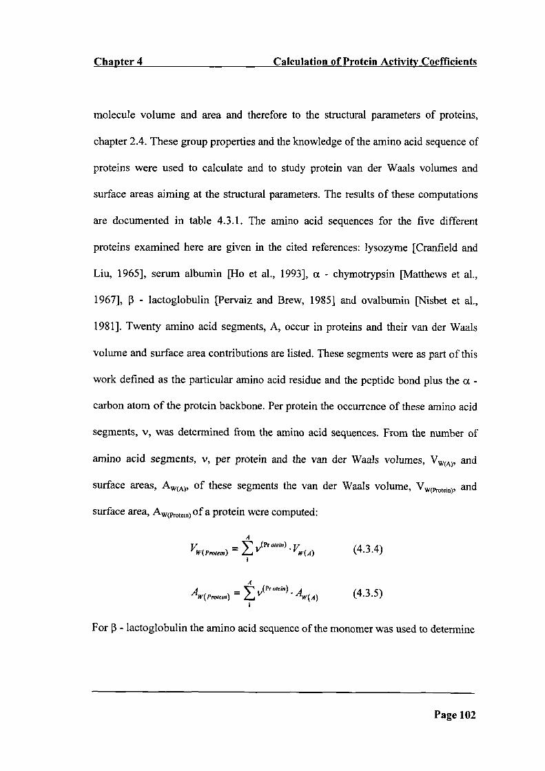
Chapter 4 Calculation of Protein Activity Coefficients
molecule volume and area and therefore to the structural parameters of proteins,
chapter 2.4. These group properties and the knowledge of the amino acid sequence of
proteins were used to calculate and to study protein van der Waals volumes and
surface areas aiming at the structural parameters. The results of these computations
are documented in table 4.3.1. The amino acid sequences for the five different
proteins examined here are given in the cited references: lysozyme [Cranfield and
Liu, 1965], serum albumin [Ho et al., 1993], a - chymotrypsin [Matthews et al.,
1967], - lactoglobulin [Pervaiz and Brew, 1985] and ovalbumin {Nisbet et al.,
1981]. Twenty amino acid segments, A, occur in proteins and their van der Waals
volume and surface area contributions are listed. These segments were as part of this
work defined as the particular amino acid residue and the peptide bond plus the a -
carbon atom of the protein backbone. Per protein the occurrence of these amino acid
segments, v, was determined from the amino acid sequences. From the number of
amino acid segments, v, per protein and the van der Waals volumes, W(A)' and
surface areas, Aw(A), of these segments the van der Wants volume, VWotejfl), and
surface area, Aw(otejfl) of a protein were computed:
A
VW(p, ) = v°"' . Vw( A) (4.3.4)
A'ç' (Prolein)
AW(P) = v . Aw(A) (4.3.5)
For 3 - lactoglobulin the amino acid sequence of the monomer was used to determine
Page 102

Chapter 4 Calculation of Protein Activity Coefficients
Table 4.3.1: Calculated van der Waals volumes and surface areas of proteins
A VW(A) AW(A) V V V V V
[A3] [A2] LYS S C L* 0Glycine 48.4 59.6 12 19 24 4 19
Alanine 65.4 83 12 58 22 15 35
Valine 99.2 127.3 6 33 23 9 31
Leucine 116 148.2 8 69 19 22 32
Isoleucine 122.5 148.2 6 14 10 10 25
Serine 72.5 89.8 10 34 27 7 38
Threonine 89.5 113.2 7 28 22 8 15
Cystein 84.5 104.7 8 35 10 5 6
Methionine 116.9 146.4 2 1 2 4 16
Proline 93.5 112.3 2 30 9 8 14
Aspartic acid 90.7 113.9 8 41 8 10 14
Asparagine 95.6 119.3 13 11 14 5 17
Glutamic acid 107.5 134.8 2 58 4 16 33
Glutamine 112.4 140.2 3 17 10 9 15
Lysine 127.8 159.7 6 62 14 15 20
Arginine 143.3 172.6 11 25 3 3 15
Histidine 109 113.5 1 19 2 2 7
Phenylalanine 136 165.4 3 33 6 4 20
Tyrosine 148.6 184.7 3 18 12 4 10
Tryptophan 166.4 193.7 6 2 0 2 3
VW(prote,n) [A3] - - 12897 62545 22812 16859 39144
AW(J CIfl) [A2] - - 15930 77578 28460 20995 48572
A: amino acid segments, LYS: lysozyme, S: serum albumin, C: a - chymotrypsin, L:
- lactogobulin monomer, 0: ovalbumin
Page 103
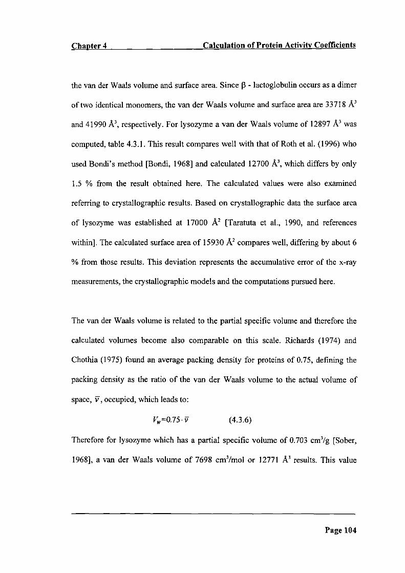
Chapter 4 Calculation of Protein Activity Coefficients
the van der Waals volume and surface area. Since 3 - lactoglobulin occurs as a dimer
of two identical monomers, the van der Waals volume and surface area are 33718 A3
and 41990 A3 , respectively. For lysozyme a van der Waals volume of 12897 A 3 was
computed, table 4.3.1. This result compares well with that of Roth et a!. (1996) who
used Bondi's method [Bondi, 19681 and calculated 12700 A 3 , which differs by only
1.5 % from the result obtained here. The calculated values were also examined
referring to crystallographic results. Based on crystallographic data the surface area
of lysozyme was established at 17000 A2 [Taratuta et al., 1990, and references
within]. The calculated surface area of 15930 A2 compares well, differing by about 6
% from those results. This deviation represents the accumulative error of the x-ray
measurements, the crystallographic models and the computations pursued here.
The van der Waals volume is related to the partial specific volume and therefore the
calculated volumes become also comparable on this scale. Richards (1974) and
Chothia (1975) found an average packing density for proteins of 0.75, defining the
packing density as the ratio of the van der Waals volume to the actual volume of
space, %7, occupied, which leads to:
(4.3.6)
Therefore for lysozyme which has a partial specific volume of 0.703 cm 3/g [Sober,
1968], a van der Waals volume of 7698 cm 3/mol or 12771 A3 results. This value
Page 104

Chapter 4 Calculation of Protein Activity Coefficients
compares well to the calculated value of 12897 A 3 , table 4.3.1, and differs by only
about 1 %. The same procedure was followed for three other proteins, serum
albumin, chymotrypsin and ovalbumin. From the specific volumes van der Waals
volumes of 63843 A3 , 22436 A3, and 41881 A3 resulted for the three proteins,
respectively. Comparison gave deviations of about 2 %, 2 % and 7 % for
experimentally determined and computed van der Wanis volumes and implies
accuracy for the group contribution calculations, table 4.3.1, which show an average
deviation of 3.7 %. By these means, it was shown that the correct structural
parameters were applied.
This examination was of importance as previous calculations perused as part of this
work but not presented here had resulted in model calculations that demonstrated on
average a poorer model performance than those finally reported here. For those first
calculations higher structural parameters (r higher by 7 % and q higher by 25 %)
values were applied as a less accurate method to obtain these parameters was used.
The average deviation of the calculations documented here, which were pursued with
the confirmed set of parameters, was by a factor ten lower than for those with higher
structural parameters. This illustrates the impact of the structural parameters on the
model performance and emphasises the importance of these studies.
Page 105

Chapter 4 Calculation of Protein Activity Coefficients
Investigations by Janin (1976) and Teller (1976) showed that volume and surface
properties of proteins are proportional to a protein's molecular weight. As molecular
weights of proteins are more widely available than their amino acid sequences a
prediction method for the structural parameters on the basis of molecular weights
was created. The determined van der Waals volumes and surface areas were
converted into the structural parameters, equation 2.4.6 - 7, which were correlated to
protein molecular weights. For the structural parameters a linear relationship with
protein molecular weights, M, resulted:
r = 0.0362• M (4.3.7)
q = O.0273• M (4.3.8)
For both correlations R2 of 1 resulted indicating a perfect fit and figure 4.3.1
illustrates this agreement. The protein ovalbumin was not included in the correlation
process and it was used to examine the performance of the developed equations. A
prediction error of 5 % resulted for each of the two parameters and additionally
confirms the new correlations, which also reflect the results of Janin (1976) and
Teller (1976). The developed correlations, which were developed as part of this
work, simplify the evaluation process for the structural parameters of a protein as
now calculations are possible without the knowledge of a protein's amino acid
sequence. The structural parameters of proteins were calculated using these newly
established correlations and were used for all the following model calculations, table
Page 106
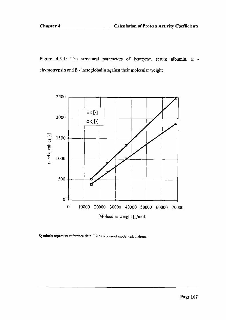
Chapter 4 Calculation of Protein Activity Coefficients
Figure 4.3.1: The structural parameters of lysozyme, serum albumin, a -
chymotrypsin and - lactoglobulin against their molecular weight
2500
2000
Ce
-I 1000
500
0
0 10000 20000 30000 40000 50000 60000 70000
Molecular weight [g!mol]
Symbols represent reference data. Lines represent model calculations.
Page 107

Chapter 4 Calculation of Protein Activity Coefficients
Table 4.3.2: UNIQUAC modelling data of protein systems
System PS I qprotein rprojn UPS i, PS I UPS I, Protein Uprotein, Protein
[g/mol] [-1 [-] [K] [K] [K]
S PS 1 68598 1873 2483 -8524.99 -8739.09 -8892.08
Cl PS2 24500 669 887 670.117 330.113 -102.052
C2 PS3 24500 669 887 766.012 398.105 -102.052
C3 PS 4 24500 669 887 825.842 439.42 1 -102.052
C4 PS 5 24500 669 887 379.094 118.679 -127.334
C5 PS 6 24500 669 887 404.658 156.54 1 -93.0088
C6 PS 7 24500 669 887 394.952 130.132 -127.334
C7 PS 8 24500 669 887 -2717.82 -2820.68 -2488.63
L P59 36800 1005 1332 538.302 241.233 -96.1955
0 PS 10 45000 1229 1629 1181.38 912.220 643.074
0.92, = 1.40
4.3.2. For the pseudo solvent the established structural parameters of water were used
in the following work.
Page 108
Chapter 4 Calculation of Protein Activity Coefficients
In addition to the structural parameters the binary interaction parameters had to be
determined to calculate activity coefficients with the UNIQUAC model. For each
system up to three binary interaction parameters were determined using a
multivariable non - linear optimisation technique of conjugate directions by Powell
[Press et al., 1986]. A minimisation of the error between calculated and experimental
activity coefficients was performed to guide the optimisation procedure. The
structure of the program is displayed in figure 4.3.2. To determine the adjustable
parameters initial values for the parameters, i.e., interaction parameters, were applied
for the first calculation step. These initial parameters were set equal to one in most
cases. Following the programming routine activity coefficients are calculated using
equation 4.3.1 - 4.3.3 and the calculated coefficients were compared to the
experimentally determined coefficients evaluating the standard square deviation,
equation 3.3.1.1. Depending on the computed deviations, i.e., objective function
values, new parameters are evaluated by the optimisation routine. This parameter
adjusting routine is applied until a minimal deviation of computed and
experimentally determined activity coefficients is obtained, which gives optimal
parameters and lowest deviation between experimental and computed data. The
programming routine developed and applied for this work is given in appendix B.
Page 109

Chapter 4 Calculation of Protein Activity Coefficients
Figure 4.3.2: Programming structure used to determine interaction parameters
START
'If
experimental data
T *X, '' 1 Protein
'If
initial values
= 1
calculate Y* Protein <
(original LJNIQUAC model)
'If
Powell's Method: optimise u
OBJ = [rx. _r:ai.J2
I Yexp.
New u.Mi OBJ
1,
.1-
results
'If
END
x: mole fraction, T: temperature, y: activity coefficient, U: interaction parameter, i and j: compound,
OBJ: objective function, N: number of data points, exp.: experimental, cal.: calculated
Page 110

Chapter 4 Calculation of Protein Activity Coefficients
From this optimisation routine three model parameters, the interaction parameters u,
resulted per system, table 4.3.2. These parameters represent the different interactions
occurring between the compounds, i.e., the pseudo solvent and the protein. For
different a - chymotrypsin systems the same protein - protein interaction parameter
was determined when system pH and temperature are the same, table 4.2.1. This is
the case for systems Cl, C2 and C3, and likewise for systems C4 and C6. For all
other systems, the same does not hold as system conditions differ.
A root mean square deviation of 0.54 % between experimentally determined and
calculated activity coefficients is obtained for the model over all ten systems and is
documented in table 4.3.3. All systems show good agreement with the experimental
behaviour. Higher than average deviation resulted for two systems. One a -
chymotrypsin system, C3, shows higher deviation than 0.54 %, which seems due to
the more complex solution behaviour of the system as indicated by the number of
virial coefficients, table 4.2.1.1, needed to determine the solution behaviour in the
first case. The ovalbumin system, 0, shows the highest deviation with a root mean
square deviation of 2.35 %. This behaviour is possibly due to the high protein
concentration of up to 7 % mass fraction, which is highest compared to the other
systems examined. All other systems have protein mass fractions of a maximum of 5
%. Therefore, extrapolation to predict activity coefficients above protein mass
Page 111

Chapter 4 Calculation of Protein Activity Coefficients
Table 4.3.3: Performance of protein activity coefficient calculations using the
original IJNIQUAC model (unsymmetric)
System Number of data points rmsd [%]
S
27
0.54
Cl
9
0.08
C2
9
0.31
C3
9
1.65
C4
6
0.07
C5
6
0.14
C6
5
0.05
C7
6
0.19
L 15 0.03
0 7 2.35
Average 9.9 0.54
fractions of 5 % is not guaranteed with the determined parameters, which resulted
from this work.
Page 112

Chapter 4 Calculation of Protein Activity Coefficients
To judge the average root mean square deviation of 0.54 %, i.e., the model
e&& kt{cperformance, the previously established cxperimcntation error, chapter 3.3.2, was
reviewed. Activity coefficient data from different laboratories had been compared
and three protein related compounds demonstrated an average root mean square
£ec1i atckdeviation of 1.8 %. Comparison of this cxperimcntation error of 1.8 % and the model
deviation of 0.54 % shows that the applied model performs well within the
,4.tCJ "urkcxperimcntation error.
For the seven a - chymotrypsin systems, Cl - C7, the experimentally determined
activity coefficients and calculated activity coefficients are displayed in figure 4.3.3,
4.3.4 and 4.3.5 demonstrating furthermore the good model performance.
In Figure 4.3.3 the activity coefficients of a - chymotrypsin at different ionic
strengths of potassium sulphate are shown. It is observed that with an increase of
ionic strength from 0.05 M to 0.15 M a lower activity coefficient results for a -
chymotrypsin. Activity coefficients reflect the solubility behaviour since protein
solubility is proportional to the inverse of the protein activity coefficient as discussed
by Green and Hughes (1955). This implies that the solubility of a - chymotrypsin
increases with increasing ionic strength from 0.05 M to 0.15 M, figure 4.3.3. Such a
solubility behaviour would occur in the salting - in region, where protein solubility
Page 113

1.3
1.2
1.1
1.0
0.9
0.8C0
• 0.7>U
0.6
0.55M
1.OE-05 1.5E-05 2.OE-05 2.5E-05 3.OE-05
0.4
0.OE+00 5.OE-06
Chapter 4 Calculation of Protein Activity Coefficients
Figure 4.3.3: Experimentally determined and modelled (original UNIQUAC
unsymmetric) activity coefficients of a - chymotrypsin with varying ionic strength of
potassium sulphate against protein mole fraction
Mole fraction [-1
Symbols represent the experimentally determined data. Lines represent model calculations.
Page 114
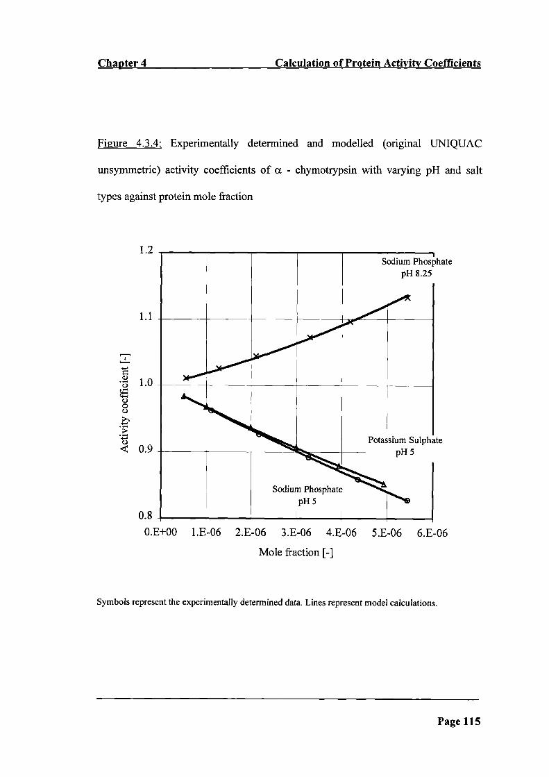
1.2
1.1
0
00
00.9
thate
.te
0.8
0.E+00 1.E-06 2.E-06 3.E-06 4.E-06 5.E-06 6.E-06
Chapter 4 Calculation of Protein Activity Coefficients
Figure 4.3.4: Experimentally determined and modelled (original UNIQUAC
unsymmetric) activity coefficients of a - chymotrypsin with varying pH and salt
types against protein mole fraction
Mole fraction [-]
Symbols represent the experimentally determined data. Lines represent model calculations.
Page 115

1.0
0.9
0.8
0.7
0.6
C0
4-.0
0.3
0.2
0.E+00 1.E-06 2.E-06 3.E-06 4.E-06 5.E-06 6.E-06
Chapter 4 Calculation of Protein Activity Coefficients
Figure 4.3.5: Experimentally determined and modelled (original UNIQUAC
unsymmetric) activity coefficients for a - chymotrypsin at different temperatures
against protein mole fraction
Mole fraction [-1
Symbols represent the experimentally determined data. Lines represent model calculations.
Page 116

Chapter 4 Calculation of Protein Activity Coefficients
increases with rising salt concentration until the salting - out region is reached where
the opposite solubility behaviour occurs. Ries - Kautt [Ducruix and Giege, 1 992}
states that generally, at salt concentrations below 0.5 M, the salting - in effect is
observed which agrees with the solubility behaviour correlated from the activity
coefficients. Comparison at the two higher salt concentrations of 0.15 M and 0.3 M,
demonstrates the shift from the salting - in towards the salting - out region where
with rising salt concentration a decrease in solubility is observed, figure 4.3.3.
In figure 4.3.4 the activity coefficients and their behaviour with respect to pH and
salt types are shown. Comparison of the activity coefficients for the systems with
sodium phosphate at different pH demonstrates that at the higher pH higher activity
coefficients result than at the lower pH. For the solubility the opposite behaviour is
deduced. The solubility is higher at a pH of 5 and lower at a pH of 8.25. It has been
established [Bailey and 011is, 1986] that proteins exhibit their lowest solubility at the
isoelectric point. For a - chymotrypsin the isoelectric point is at pH 8.25. The
solubility behaviour and activity coefficient behaviour as a function of pH suggests
therefore additionally to the examination of salt concentrations that the models are
correct.
Figure 4.3.4 also shows the activity coefficients for a - chymotrypsin as a function of
Page 117

Chapter 4 Calculation of Protein Activity Coefficients
two different salt types, potassium sulphate and sodium phosphate. The activity
coefficients at a constant pH of 5 are lower for the phosphate anions than for the
sulphate anions. A higher solubility for phosphate anions and a lower solubility for
sulphate anions results. This implies that the sulphate anion is the more effective
precipitation agent of the two anions. This behaviour is in agreement with the results
of Hofmeister (1888) on precipitation effectiveness. However, the observed
difference is small and compares also well to the result of Shih et al. (1992) who
found that the two anions have almost equivalent precipitation effectiveness on a
different protein, lysozyme.
For the protein a - chymotrypsin the temperature dependence was predicted with the
model parameters established as a result of this work, table 4.3.2. In figure 4.3.5 the
experimental data and model performance are given for three temperatures. With
increasing temperature the activity coefficients decrease which indicates that the
solubility of a - chymotrypsin rises with temperature at given conditions. By
lowering the temperature the opposite behaviour is observed. This temperature
dependence for solubility is most commonly found from experiments [Ducruix and
Giege, 1992] and hence the model prediction tendency observed is confirmed as
qualitatively correct.
Page 118

Chapter 4 Calculation of Protein Activity Coefficients
The experimentally determined activity coefficients were demonstrated to relate to
the common solubility behaviour as a function of ionic strength, pH, salt type and
temperature. By confirming the experimental data the model was approved, which
was shown to follow the experimental data with a deviation of 0.54 %.
4.4 Summary
Protein activity coefficient data has been established here from osmotic pressure
measurements for ten protein - salt - water systems. After the development of a
prediction method to obtain the structural parameters for globular proteins the
determined activity coefficient data was used to obtain a number of new IJNIQUAC
interaction parameters. These were used to support the estimation and prediction of
protein activity coefficients as a function of compound types, composition and
temperature. On average a root mean square deviation of 0.54 % resulted when the
experimentally determined data and calculated data was compared, showing that the
model follows the experimental behaviour. This demonstrated that the original
UNIQUAC model, using the interaction parameters generated and the proposed
evaluation method for the structural parameters of proteins, is applicable for the
systems and compounds of interest.
Page 119

Chapter 4 Calculation of Protein Activity Coefficients
The systems examined, protein - salt - water systems, cover a wide range of different
system conditions and therefore the different effects of these conditions on activity
coefficients were studied. Effects of salt concentrations and types, system pH and
temperature were examined. The relationship introduced for activity coefficients and
protein solubility allowed a qualitative interpretation of protein solubility with
respect to these parameters. The fact that the protein solution property, solubility, is
described correctly in a qualitative manner through activity coefficients additionally
validated the model approach. Having confirmed the model approach and shown
correct protein solubility representation through protein activity coefficients
encouraged the next part of this work where the quantitative protein solubility
description was addressed.
4.5 Nomenclature
A amino acid segments
A van der Waals area
B virial coefficient
C a - chymotrypsin
c molar concentration
D virial coefficient
L - lactoglobulin
Page 120

Chapter 4 Calculation of Protein Activity Coefficients
LYS
m
M
N
0
OBJ
PS
q
R
r
rmsd
S
t
T
U
UNIQUAC model
vw
x
lysozyme
molal concentration
molecular weight
number of data points
ovalbumin
objective function
pseudo solvent
structural area parameter of a compound
gas constant
structural volume parameter of a compound
root mean square deviation
serum albumin
temperature
temperature
interaction parameter
UNIversal QUAsi Chemical model
van der Waals volume
compound mole fraction
Greek letters
[I
Y
V
V
p
osmotic pressure
compound activity coefficient
segment occurrence
partial specific volume
density
Page 121
Superscript
*
C
R
Chapter 4 Calculation of Protein Activity Coefficients
Subscript
A
cal.
exp.
1
J
m
P
PS
amino acid segment
calculated
experimental
compound
compound
molal concentration
protein
pseudo solvent
unsymmetric
combinatorial
residual
Page 122
Chapter 5 Calculation of Protein Solubility
Chapter 5
Calculation of Protein Solubility
A modelling approach for the description of the solid - liquid equilibrium is
introduced and used to represent protein solubility for two different systems as a
function of salt concentration and temperature.
5.1 Introduction
It was demonstrated for ten systems that protein activity coefficients are well
described with the UNIQUAC model. Furthermore, it was shown that protein
solubility can be qualitatively described through protein activity coefficients, chapter
four. Therefore, the quantitative modelling of protein solubility was approached next
Page 123

Chapter 5 Calculation of Protein Solubility
and this part of the work is documented in this chapter. Protein activity coefficients
and the solubility product were used to express the solid - liquid equilibrium. Two
different globular proteins, lysozyme and concanavalin A, and two salt types, sodium
chloride and ammonium sulphate, were examined. Protein solubility for the different
systems as a function of the salt type, salt concentration and temperature was
investigated using the introduced modelling framework. This work is also presented
and discussed elsewhere [Agena et al., I 997a; Agena et al., 1 998a].
In the following part of this chapter first the solubility data of the two systems is
presented and the protein solubility behaviour of those two systems is examined. The
solubility behaviour over composition and temperature is discussed, which
introduces the salting - out region, and normal and retrograde solubility behaviour,
respectively. Thereafter, the model framework is presented and the results using this
modelling approach are discussed. To confirm the model various directions are
pursued and various verification approaches are suggested to support the solubility
model qualitatively.
Page 124

Chapter 5 Calculation of Protein Solubilitv
5.2 Experimental Solubility Data
Experimental solubility data is necessary in order to model protein solubility but
defined and extensive solubility measurements of proteins over various system
conditions are rare. Only recently, due to the interest in protein crystallisation, a rapid
technique was developed that made solid - liquid equilibrium data for proteins more
easily accessible and available.
In 1988 the column solubility method was devised by Pusey and Gernert (1988),
which gives solubility measurements from oversaturated and undersaturated protein
solutions in the presents of a crystalline phase at constant system conditions within a
typical error of 3 % [Pusey and Munson, 1991]. Up to 100 - 200 mg of crystalline
protein [communication with Pusey, 1997] are used for a mini - column to pursue the
measurements. For two proteins, lysozyme (LYS) and concanavalin A (CON), the
solid - liquid equilibrium has been measured using this micro - column technique
[Pusey and Munson, 1991].
A selection from these measurements was utilisecl here for the model studies and is
documented in table 5.2.1. The experimental solubility data was screened and
converted to the thermodynamic scale, chapter 3.2, and the resulting data is listed in
Page 125

Chapter 5 Calculation of Protein Solubility
appendix D. Experimental solubility data for aqueous protein systems that are
crystallised by monovalent or divalent salts was studied while salt concentrations and
temperatures vary. The first system, I, of aqueous lysozyme (M 14600 g!mol) is a
model system and has been studied extensively. The second system, II, introduces
concanavalin A with ammonium sulphate as a crystallisation agent, which is the
dominant salting - out agent used. With its high molecular weight of 102668 g/mol,
concanavalin A is representative of the macromolecular character of proteins.
Additionally, the concanavalin A molecule is a dimer allowing for examination of a
protein consisting of two subunits, while previously 3 - lactoglobulin was
representatively studied for this characteristic when protein activity coefficients were
examined in chapter four.
Table 5.2.1: Protein systems and system conditions investigated
System Protein M Salt Buffer pH t
[g/mol]
[-] [°C]
I LYS 14600
NaC1
Sodium acetate 4 2 - 25
0.2 - 45 g/L 0.3, 0.5, 0.7, 0.9, 1.2 M 0.1 M
II
CON 102668 (NH4)2SO4 tris - acetate 6 18 - 45
0.3 -5.5gfL 0.25,0.5,1 M0.1 M
Page 126

Chapter 5 Calculation of Protein Solubility
The lysozyme (tetragonal crystal form) data had been obtained at a constant pH of 4
in 0.1 M sodium acetate buffer, while temperature and sodium chloride concentration
were varied [Cacioppo and Pusey, 1991]. The solubility behaviour as a function of
five salt concentrations from 2 % - 7 % (0.3 - 1.2 M) and in a temperature range from
about 2 - 25 °C had been obtained. For the second system, concanavalin A (acid
treated and recalcified), the solubility had been investigated using ammonium
sulphate as a salting - out agent [Cacioppo and Pusey, 1992]. Solubility data had
been determined for concanavalin A over three salt concentrations, 0.25, 0.5 and 1
M, and was examined here over the measured temperature range of 18 - 45 °C at pH
6 in 0.1 M tris - acetate buffer.
The chosen solubility data represents normal and retrograde solubility behaviour and
the salting - out region. In figures 5.2.1 and 5.2.2 the experimental data of the two
systems is shown. Figure 5.2.1 shows the solubility of lysozyme as a function of
temperature and sodium chloride concentration. A normal solubility, i.e., increasing
with temperature, is observed. Concanavalin A, figure 5.2.2, shows the opposite
behaviour. At low temperature ranges retrograde solubility, i.e., decreasing with
temperature, is observed, which is thought to occur when ammonium sulphate is
applied [Jakoby, 1968]. However, at higher temperature ranges normal solubility
behaviour is also found for the concanavalin A system. In all systems the salting - out
Page 127

7.OE-05
6.OE-05
5.OE-05
4.OE-05
3.OE-05
0.)
0
2.OE-05
1 .OE-05
O.OE+OO
Mr.44
M
Chapter 5 Calculation of Protein Solubility
Figure 5.2.1: Experimental solubility of lysozyme at various sodium chloride
concentrations against temperature
275 280 285 290 295 300
Temperature [K]
Symbols represent the experimentally determined data.
Page 128

2.OE-07
I AAa&40.OE+00
290 295
Chapter 5 Calculation of Protein Solubility
Figure 5.2.2: Experimental solubility of concanavalin A at various ammonium
sulphate concentrations against temperature
1 .2E-06
0.25 M
1 .OE-06
.
8.OE-07•U.
uu.i.uIII
6.OE-070E
• 4.OE-07 0.5 M
1M
.. ..• .AAA4AAAA
AA
300 305 310 315 320
Temperature [K]
Symbols represent the experimentally determined data.
Page 129

ChapterS Calculation of Protein Solubility
region was studied, which is demonstrated by a solubility decrease with increasing
salt concentration.
5.3 Solid - Liquid Equilibrium Model
To model protein solubility the solution behaviour and the exchange of liquid and
crystal protein between the liquid and solid phase needs to be described. The transfer
of protein between the two phases was represented by the solubility product, which is
a function of temperature while the solution behaviour, i.e., deviation from ideal
solution behaviour, was accounted for and described by the previously examined
UNIQUAC model, chapter four. In figure 5.3.1 the solubility model which consists
of these two terms is shown. These terms are the phase equilibrium and solution
activity coefficient description, which are discussed below. A programming code for
the solubility model including the parameter determination routine and solubility
calculation routine was developed as part of this work and is given in appendix E.
The phase equilibrium term, figure 5.3.1, is introduced to describe the exchange of
crystalline and liquid protein between the two phases, i.e., the solid and liquid phase,
respectively:
Page 130
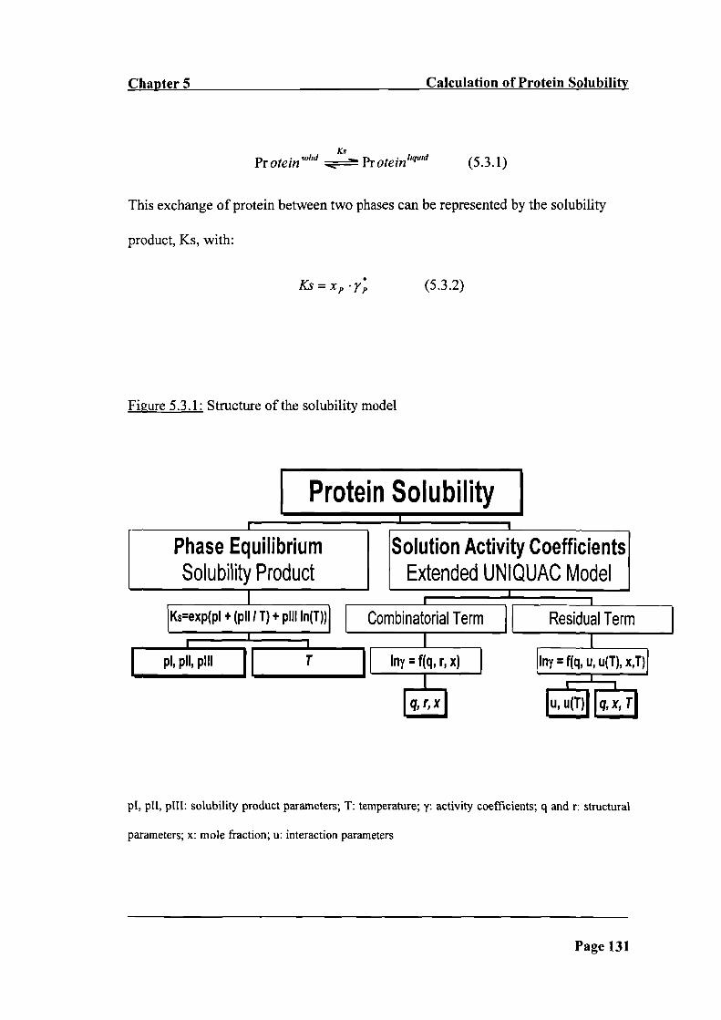
(5.3.2)
Chapter 5 Calculation of Protein Solubility
KsProtein coM . - (5.3.1)
This exchange of protein between two phases can be represented by the solubility
product, Ks, with:
Figure 5.3.1: Structure of the solubility model
Protein Solubility
Phase Equilibrium
Solution Activity CoefficientsSolubility Product
Extended UNIQUAC Model
Ksexp(pl + (pill T) + pill in(T))
combinatorial Term
Residual Term
p1, p11, pill
T
lnyf(q,r,x) I
my f(q, U, u(T), x,T)
Iq, r, x u, u(T)l Iq,x, T
p1, p11, pill: solubility product parameters; T: temperature; y: activity coefficients; q and r: structural
parameters; x: mole fraction; U: interaction parameters
Page 131

Chapter 5 Calculation of Protein Solubility
This equation, 5.3.2, relates the solubility product to the mole fraction of liquid
protein, x , which is the protein solubility. Furthermore, the liquid activity
coefficient of the protein, y4' on the unsymmetric convention y"—* 1 as x, —* 0 is
introduced in equation 5.3.2. The solubility product, Ks, is represented by the
following expression:
P'1lnKs=pI+—-+pIII . ln(T) (5.3.3)
The solubility product is a function of temperature, T. The adjustable parameters, p1,
p11 and pill, describe the solubility product and the given expression is a widely and
successfully applied description for the solubility product [Mullin, 1993, and
references within].
The solution activity coefficient term, figure 5.3.1, is introduced to describe the
protein activity coefficient introduced in equation 5.3.2. For the calculation of
activity coefficients the extended UNIQUAC model introduced by Sander et al.
(1986) was used. This model relates closely to the original UNIQUAC model, which
was shown as part of this work to describe protein activity coefficients, chapter four.
In this model the excess Gibbs energy and therefore the activity coefficients are
likewise represented by a set of two terms, a combinatorial term and a residual term:
lny, =1n71c +lny11(5.3.4)
Page 132

Chapter 5 Calculation of Protein Solubility
where
lny, =f(q,,r,,x,) (5.3.5)
lny,R =f(q,,x,,u,T) (5.3.6)
The combinatorial term, inyC, describes the entropy state of solution and is the
combinatorial term introduced for the original UNIQUAC model, chapter 2.3.1. The
composition of the system is introduced with the mole fraction, x, while the
structural parameters, q and r, represent the size and shape of the compounds
accounting for the differences of small molecules and macromolecules. The
structural parameters of the studied compounds are summarised in table 5.3.1. For
the salt ions the structural parameters were obtained from literature [Sander et al.,
1986; Pessoa et al., 1992]. In the case of the sodium ion the structural parameters
were calculated from the ionic radius as given by Pauling (1960). The structural
parameters of the proteins were calculated from the protein molecular weights using
the method developed as a result of this work, chapter 4.3. For the water related
compounds, i.e., the pseudo solvents, the established structural parameters of water
were applied [Abrams and Prausnitz, 1975].
Page 133

Chapter 5 Calculation of Protein Soinbility
Table 5.3.1: Structural parameters of proteins, salt ions and pseudo solvents
Compound r [-] q [-1
Lysozyme 529 399
ConcanavalinA 3717 2803
Na 0.1425 0.2731
Cl 0.9861 0.9917
NI-140.9097 0.9800
SO422.3138 1.3600
PS 1 0.92 1.4
PS2 0.92 1.4
Two pseudo solvents, PS, were introduced as two different, protein buffers were
applied over the two systems: PS 1 and PS 2 referring to system I and II,
respectively. Effects of buffer concentration and therefore type have been shown to
markedly affect protein solubility [Forsythe and Pusey, 1996] and were hence
incorporated by creation of a pseudo solvent. The introduction of pseudo solvents has
been established for the previous calculations on protein activity coefficients, chapter
Page 134

Chapter 5 Calculation of Protein Solubility
four, and was therefore adapted again. This concept was applied as it reduces the
number of compounds per system and therefore the number of parameters needed.
This is especially of interest with respect to the binary interaction parameters which
have to be determined and their number rises with the number of system compounds,
equation 2.4.10. Minimisation of system compounds reduces the number of
parameters to be determined but it also reduces the predictive power of the model.
Introduction of the solvent and buffer as independent compounds would have
allowed for predictions over buffer concentration. However, the data used here is
constant over the buffer concentration and therefore a prediction over the buffer
concentration would not have been advisable even if possible.
While the combinatorial term is that of the original model the residual term, Iny', was
extended by Sander et al. (1986) and resembles that also introduced with the
modified model, equation 2.6.3. However, for this work only the first two
temperature terms were introduced for the interaction parameters, u:
uIJ =u;+u.(T-3oo) (5.3.7)
Termination after the second term leads to less secondary interaction parameters per
binary interaction parameter, which was an objective as less parameters had to be
determined. To describe the behaviour of the studied four compound systems, protein
- cation - anion - pseudo solvent, the secondary binary interaction parameters, u° and
Page 135

Chapter 5 Calculation of Protein Solubility
Ut had to be determined.
5.4 Study of the Solubility Model
In order to model protein solubility for the two systems the values of the solubility
product parameters and the interaction parameters had to be determined. The
program routine in appendix E was designed for this purpose and performs similar to
the one described in chapter 4.3. An Indigo2 Impact (195 MHZ 1P28 Processor,
CPU: MIPS Ri 0000 Processor Chip Revision: 2.5, Secondary unified
instruction/data cache size: 1 Mbyte, Main memory size: 64 Mbytes) performing at
124.4 Whetstone MIPS was used for the parameter determination and solubility
calculation. The experimental solubility data was used to guide the determination
while the thermodynamic functions, equations 5.3.2, 5.3.3 and 5.3.4, were estimated,
minimising the following objective function:
* 2
expN ( —X01(K,7 )
J(5.4.1)ssd = LI X9
The multivariable non - linear optimisation technique of conjugate directions by
Powell [Press et al., 19861 was adopted to minimise the standard square deviation,
ssd. The deviation of experimental solubility, Xexp, and modelled solubility, x, over
Page 136

Chapter 5 Calculation of Protein Solubilitv
all data points, N, was minimised. The solubility is calculated as a function of the
solubility product, Ks, arid the protein activity coefficients, y*, while the solubility
product parameters and interaction parameters are optimised.
From the optimisation procedure the parameters, p1, p11 and pill, of the solubility
product resulted. The parameters determined as a result of this work are listed in
table 5.4.1. For each of the two systems one crystal form was represented, leading to
one solubility product per system over the temperature range. In the case of lysozyme
it has been established that only the tetragonal crystal form occurs under the studied
conditions [Cacioppo and Pusey, 1991; Ewing Ct al., 1994]. Calculations at higher
temperatures would require the solubility product relating to the orthorhombic crystal
form of lysozyme. For the other system, concanavalin A, it has not been shown that
Table 5.4.1: Parameters of the thermodynamic solubility product for lysozyme and
concanavalin A
Solid phase p1 p'1 * (y3 pill temperature range [°C]
Lysozyme 17.9891 -3.966148 -2.3381
2-25
Concanavalin A -2289.08 113.390
333.270
18 - 45
Page 137

Chapter 5 Calculation of Protein Solubilit'v
only one crystal form exists under the conditions studied but experimental indication
for various crystal forms have not been found during the experimental solubility
studies [communication with Pusey, 1996].
In addition to the solubility product parameters, the binary interaction parameters
were determined. For the studied systems the interaction parameters are given in
tables 5.4.2 and 5.4.3. For the salt total dissociation was described leading to two
ions and producing a four compound system. This approach was taken for the salt as
previous examinations of the model with a non dissociating salt and therefore a three
compound system did not succeed. Deviations were by a two or three - fold higher
than found for modelling approaches with a dissociating salt, i.e., four compound
system. As ions show different impacts on the crystallisation process as discussed
later this concept is supported. Furthermore, representation of the salt as ions is a
realistic representation as this occurs in solution. However, the three compound
systems was examined in order to reduce the number of interaction parameters as
discussed before. Still, as a result of this approach systems consisting of four
compounds - protein, cation, anion, pseudo solvent- were modelled and up to twelve
binary interaction parameters were determined. Insignificant interaction parameters
were indicated during the optimisation process. An independence of the parameter
values and the calculated solubility was observed. These interaction parameters did
Page 138

Chapter 5 Calculation of Protein Solubility
Table 5.4.2: Binary interaction parameters for the lysozyme system
u°1 [K] PS 1 Lysozyme Na CFPS 1 -3210.69 -3217.27 -3763.78 -3723.26
Lysozyme
0 0 -3543.58
Na 0 0
cr 0
u t.. [ ..j PS 1 Lysozyme Na CiPS 1 0 0.0123 0 2.1818
Lysozyme 0 0 4.3890Na 0 0
CF 0
Table 5.4.3: Binary interaction parameters for the concanavalin A system
u0 [K] PS 2 Concanavalin A NH4 so42PS2 53.10 10.18 -401.07 21.48
ConcanavalinA 1012.89 20.12 619.05
NFI40 0
So42-0
u tjj j PS 2 Concanavalin A NH4 So42
PS 2 0 0.3977 -1.2626 4.6523Concanavalin A 0 5.4760 6.8900
NH40 0SO420
Page 139

Chapter 5 Calculation of Protein Solubility
not seem to be of significance for the solubility process and were therefore adjusted
to values of zero indicating no interactions. This approach is further discussed and
related to the findings of other researchers.
For system I, consisting of lysozyme and sodium chloride, a number of binary
interaction parameters are not relevant. The lysozyme - lysozyme interactions and
ion - ion interactions are of minor importance. The interactions of the pseudo solvent
and chloride with the other compounds are predominant, table 5.4.2. The strong
effect of the chloride anion and low impact of the sodium cation reflected in the
model has also been noted by Taratuta et a!. (1990). They demonstrated
experimentally that cation substitution had no effect on the lysozyme coexistence
curve while anion substitution had. Likewise, the greater impact of anions over
cations on protein solubility was shown by Hofmeister (1888) and recently
confirmed by Carbonnaux et al. (1995). While this behaviour was proven through
experiment by various researchers it was here for the first time, to the best of my
knowledge, shown by theory and the same applies for the next case. For the second
system of concanavalin A more than eight interaction parameters had to be
determined. While the ion - ion interactions are also irrelevant the cation certainly
has an impact and is not to be neglected as in the lysozyme system. This relates to
Jakoby's finding (1968), who demonstrated that aminonium sulphate leads to the
Page 140

Chapter 5 Calculation of Protein Solubiijy
retrograde solubility behaviour. Furthermore, it implies that ammonium and sulphate
ions and not only e.g. the sulphate ions induce the retrograde solubility behaviour.
With the determined parameters protein solubility was calculated as a function of
temperature and salt concentration. In figures 5.4.1 and 5.4.2 the modelled and
experimental solubility data is shown. These figures demonstrate qualitative
agreement of model and experimental behaviour. Correspondingly, the quantitative
comparison gives good results. Comparison of the experimental solubility data and
the model calculations gives a root mean square deviation of 7 % for lysozyme, table
5.4.4. This is slightly above the deviation range, 3.9 - 5.7 %, reported by Cacioppo
and Pusey (1991) for their polynomial correlations over the temperature range alone.
The deviation of the solubility model, however, included deviations due to
temperature and composition. For the concanavalin A system the deviation of
experimental and modelled solubility as a function of salt concentration and
temperature is 4.5 %. Overall an average deviation of 5.8 % resulted for the systems
when the model calculations and experimental solubility data was compared showing
that the model follows well the experimental behaviour of two different systems.
For the two systems the activity coefficient calculations were also examined and used
as constraints to direct the applied framework and secure its validity. In figure 5.4.3
Page 141

6.OE-05
5 .OE-05
4.OE-050C)
0
C)
0
3 .OE-05
2.OE-05
1 .OE-05
O.OE+OO
Chapter 5 Calculation of Protein Solubility
Figure 5.4.1: Experimental and modelled solubility of lysozyme at five different
sodium chloride concentrations against temperature
4
444
275 280 285 290 295 300Temperature [K]
Symbols represent experimentally determined data. Lines represent model calculations.
Page 142

Chapter 5 Calculation of Protein Solubility
Figure 5.4.2: Experimental and modelled solubility of concanavalin A at different
ammonium sulphate concentrations against temperature
I .2E-06
1 .OE-06
8.OE-07
6.OE-07
4.OE-07
2.OE-07
0. OE+00
290 295 300 305 310 315 320
Temperature [K]
Symbols represent experimentally determined data. Lines represent model calculations.
Page 143

Chapter 5 Calculation of Protein Solubility
Figure 5.4.3: Modelled activity coefficients of lysozyme at different sodium chloride
concentrations against temperature
400
350
300
250
200
: 150
100
50
0Li lvi
275 280 285 290 295
300
Temperature [K
Lines represent model calculations.
Page 144

Chapter 5 Calculation of Protein Solubility
Table 5.4.4: Performance of solubility calculations for lysozyme and concanavalin A
using the solid - liquid equilibrium model
System N ssd, objective function value rmsd %]
Lysozyme 93 0.45 7.0
ConcanavalinA 93 0.19 4.5
Average 93 - 5.8
the calculated activity coefficients of lysozyme against temperature and the salt
concentrations are given. The activity coefficients show a 2 fold decrease over the
rising temperature range while a 20 fold increase is found over the increasing salt
concentration range indicating the impact of these factors on protein solubility for the
studied cases.
The qualitative behaviour of the activity coefficients, figure 5.4.3, relates correctly to
the experimental solubility behaviour following the fact that activity coefficients are
inversely proportional to the solubility at constant temperature, equations 5.3.2 and
5.3.3. The activity coefficients increase with an increase in salt concentration
Page 145

Chapter 5 Calculation of Protein Solubility
indicating the opposite solubility behaviour, i.e., salting - out behaviour, as found by
experiment. The correct solubility behaviour is also deduced with respect to the
temperature dependence. This indicates that activity coefficients of proteins represent
qualitatively correctly the protein solubility behaviour but also that the model
constraint for the activity coefficient calculations was obeyed.
Still, it could not be validated that the activity coefficient results are quantitatively
correct. Similar magnitudes for activity coefficients were reported by Ross and
Minton (1977) for haemoglobin. They reported values for activity coefficients from
about I to about 580 over a concentration range of 20 - 400 g/L and comparable
quantitative results were obtained for activity coefficients from this model but system
conditions are different to the ones studied by Ross and Minton (1977). Therefore,
the quantitative results for the protein activity coefficients were not validated while
likewise not proven wrong. However, model consistency was additionally shown by
means of the qualitative behaviour of the intermediate solution property, protein
activity coefficient.
Page 146

Chapter 5 Calculation of Protein Solubility
5.5 Summary
It has been demonstrated that the chosen model approach represents protein solubility
for two globular proteins of very different size, lysozyme and concanavalin A. Their
solubility as a function of added salt concentration and system temperature was
studied. The salting - out region, normal and retrograde solubility behaviour of these
proteins was modelled. For each of the four compound systems - protein, cation,
anion, pseudo solvent - a the minimal number of parameters was determined as part
of this work by setting insignificant interaction parameters equal to zero. Using the
determined parameters the solubility over the given conditions was calculated and an
average deviation of 5.8 % resulted for the proposed model approach when compared
to the reference solubility data. To examine the model framework in more detail
additionally the calculated protein activity coefficients were viewed and showed to
correlate qualitatively correct to the experimental solubility behaviour. Furthermore,
some of the determined parameters confirmed the model while likewise for the first
time experimental findings were validated using this theoretical approach.
Page 147

Chapter 5 Calculation of Protein Solubility
5.6 Nomenclature
CON
Ks
LYS
M
N
p1
p'1
pill
PS
q
r
rmsd
ssd
t
T
U
UNIQUAC model
x
Greek letters
I
Subscript
cal.
concanavalin A
solubility product
lysozyme
molecular weight
number of experimental data points
solubility product parameter
solubility product parameter
solubility product parameter
pseudo solvent
structural area parameter of a compound
structural volume parameter of a compound
root mean square deviation
standard square deviation
temperature
temperature
interaction parameter
UNIversal QUAsi Chemical model
compound mole fraction
compound activity coefficient
calculated
Page 148
Chapter 5 Calculation of Protein Solubility
exp. experimental
compound
compound
protein
Superscript
* unsymmetric
C combinatorial
R residual
t temperature
Page 149

Chapter 6 Conclusions
Chapter 6
Conclusions
This chapter summarises the contributions and conclusions of the presented research
project.
1. In this work for the first time systematic studies of activity coefficient predictions
were pursued and documented for amino acids and peptides using the predictive
power of the UNIFAC method and the parameters of Hansen et a!. (1991). To
study the predictive capacities of this method the UNIFAC groups, model
parameters, model versions and activity coefficient reference states were
examined. Amino acids and peptides were studied assuming that a model that is
successful for these compounds will also be successful for proteins and vice
versa. This was assumed as the first set of compounds, amino acids and peptides,
Page 150

Chapter 6 Conclusions
are the building blocks of proteins and therefore resemble many of a protein's
characteristics such as interactions but not size.
2. For the first time the most extensive and recent UNIFAC group and parameter
database of Hansen et a!. (1991) was applied to describe activity coefficients of
amino acids and peptides using the UNIFAC model. It was demonstrated with
this work that the group definitions are not appropriate for peptides and therefore
proteins. A molecular representation of the peptide bond occurring between two
different amino acids in an amino acid sequence, i.e., peptide or protein, is
missing. A description of a peptide's and protein's backbone is lacking. This was
a first indication arising from this work suggesting that the UNIFAC model
might be at present limited in its predictive powers when aiming at amino acids,
peptides and proteins. Compounds closely related to these were not used to
establish the model parameters and therefore a proper description of their
properties is less likely to occur.
3. The examination of the database of Hansen et al. (1991) was taken further in this
work. It was shown that certain binary interactions, which typically occur for
amino acids, peptides and proteins, are not accounted for. Interactions of the
amino terminus with the carboxyl terminus and the carboxyl groups of the acidic
Page 151

Chapter 6 Conclusions
residues, aspartic acid and glutamic acid, are not established. However, these
molecular groups are very likely to interact when in the vicinity of each other as
they carry opposing polarities. Therefore, it was demonstrated with this work that
the predictive abilities of the UNIFAC model using the database of Hansen et al.
(1991) are limited for the systems aimed at, i.e., protein systems, due to
incomplete interaction descriptions.
4. Furthermore, two different UNIFAC models, the original and modified one, were
investigated in this work. The ability of these two models to predict activity
coefficients of protein related compounds, i.e., amino acids and peptides, was
examined. A poor predictive performance resulted for both models. Both the
original UNTFAC and the modified UNIFAC model performed unsatisfactorily
on the symmetric reference scale. Comparison of the computed activity
coefficients and those determined from experiment showed qualitative
disagreement and quantitative differences of around a 100 %. This indicated that
possibly the model approaches are not appropriate for the studied systems and for
related systems such as protein systems. However, no clear conclusion could be
drawn as too many additional factors such as possibly incorrect group definitions
and missing interaction parameters influenced the model performance. This
indicated that a model such as the UNIQUAC model, i.e., a model with no group
Page 152

Chapter 6 Conclusions
contribution method, which therefore uses less parameters was needed to clarify
the performance of the model approach.
5. Moreover, for the first time the two activity coefficient reference states, Raoult's
law and Henry's law, were studied for amino acid and peptide activity coefficient
calculations when using the original UNIFAC model. As a result of this work it
was demonstrated that the unsymmetric reference state, i.e., Henry's law, should
be used for amino acids and peptides and therefore possibly also for proteins
following the previously suggested hypothesis. The conclusion to refer to Henry's
law arose not only from this work but was also shown independently when
protein adsorption experiments were pursued by Fraaije et a!. (1991). They
demonstrated that deviation from ideal behaviour has to be expressed with
respect to Henry's law for proteins, which agrees with the result of this work and
confirms the hypothesis that amino acids, peptides and proteins relate to some
extent. Using two completely different approaches the necessary reference state
was defined. This part of the work was significant as it demonstrated that the
unsymmetric convention is to be applied for further modelling work with proteins
and related compounds.
6. Overall an essential contribution was made with this work as it showed that the
Page 153

Chapter 6 Conclusions
UNIFAC model and the most recently established groups and parameters of
Hansen et at. (1991) are not applicable to amino acid, peptide and protein systems
even though compounds related to biotechnology had been examined by Hansen
et at. (1991). The predictive power of the 1JNIFAC model with the suggested
parameters failed for the studied systems, which was demonstrated by
inappropriate predictions. However, this part of the work did not rule out the
UNIFAC model or its model base for the examined compounds but it
demonstrated the inapplicability of the UNIFAC model with the parameters of
Hansen et al. (1991).
7. Moreover, it was illustrated in this work that the UNIFAC model is not yet
applicable as too little experimental data is available to establish a reliable model.
This was discussed using the results of Pinho et a!. (1994). Due to the model's
group contribution approach more parameters need to be determined which
requires more experimental data then generally available for the systems targeted
in this work. The related UNIQUAC model overcomes this problem. It uses less
parameters and therefore requires less experimental data which is a limiting
factor and therefore of importance for this work.
8. Furthermore, it was argued in this work that the UNIQUAC model is the
Page 154

Chapter 6 Conclusions
appropriate model to study the model approach. It was pointed out in this work
that the UNIQUAC model is more easily interpreted for its performance then the
UNIFAC model as fewer parameters are required and no group information is
introduced. Therefore, sources for model deviations are reduced for the
UNIQUAC model when compared to the UNIFAC model. Following this, closer
model approach examinations are possible using the UNIQUAC model as
deviation due to those other factors are screened out. Hence, further research
work focused on the UNIQUAC model as correlations using the UNIFAC model
seemed less favourable even though the predictive power for different but related
compounds is lost using the UNIQUAC model.
9. Further model investigations pursued as part of this work focused on the
IJNIQUAC model as model approach examinations were a primary objective. As
the UNIQUAC model and the UNIFAC model use the same model approaches it
can be assumed that any confirmation of the UNIQUAC modelling approach for
protein systems is also extendible to the UNIFAC model. However, to transfer
any successful model approach from the UNIQUAC model to the UNIFAC
model the additional group contribution method would need to be addressed.
Still, as a first step it was necessary to confirm the model approach and this was
achieved with the examinations pursued in this work. In order to study the
Page 155

Chapter 6 Conclusions
UNIQUAC model interaction parameters were determined to describe the activity
coefficients of glycine, proline and glycylglycine in water. Seven new parameters
resulted from this work and therefore allowed for activity coefficient calculations.
10. Following the establishment of these parameters the original I.JNIQUAC model
was applied on the unsymmetric scale. The unsymmetric scale was applied due to
the findings that resulted from this work. Computation of activity coefficients for
two amino acids, glycine and proline, and one peptide, glycyiglycine, were
successful when using the newly determined interaction parameters and the
UNIQUAC model. With this work it was shown that on average deviations as
low as 0.2 % (in the worst case up to 0.3 %) would result for the examined
systems and the model approach used when comparing calculated activity
coefficients and experimentally determined ones. This implied that the modelling
approach is correct and that the same one should be successful for the UNIFAC
model as both models have a common theoretical base. Furthermore, this part of
the work implied that the model should also be applicable for proteins, the target
compounds, as these are closely related to the examined amino acids and peptide.
With this part of the work a possible protein modelling approach was established,
which was a first significant step towards the modelling of protein properties.
Page 156

Chapter 6 Conclusions
a bA11. Additionally, ai cAperirncntation error was established from this work for
activity coefficients in order to create an indicator for the model performance of
becLtactivity coefficient models. An average deviation of 1.8 %, i.e., cxperimcntation
error, resulted for activity coefficients from two different sources when compared
over the composition for three different protein related compounds. This error of
1.8 % for two different sources, i.e., laboratories, gave a measure for model
a,4 -kperformances, i.e., the model deviations. With an cxperimcntation error of 1.8 %
for activity coefficients over composition it was established that similar errors
should result from the models indicating that the models perform properly and
follow the experimentally determined behaviour.
h1J12. Comparison of the cxperimcntation error of 1.8 % and the average UNIQUAC
model deviation of 0.2 %, demonstrated that the model performed very well for
amino acid and peptide activity coefficients as the deviation is well below the
IXMCI nitr4cxperimcntation error. This work showed that the model described the
experimentally determined activity coefficient behaviour very well for the studied
systems and compounds. As these compounds relate to proteins a model
performance comparable to this one is expected for proteins.
13. For the first time for ten different systems and four different proteins, serum
Page 157

Chapter 6 Conclusions
albumin, a - chymotiypsin, - lactoglobulin and ovalbumin, activity coefficient
data was made available to pursue this research work further. The data was
obtained from osmotic pressure measurements documented in the literature.
Protein activity coefficients were made available over varying system
composition and over various system conditions such as compound types,
temperature and pH using virial expansion. Protein property data over a variety of
conditions resulted from this work. To obtain this data was a significant
contribution as no such comprehensive data was previously available for proteins.
This data allowed for a detailed and systematic examination of protein property
models.
14. As a next step in the pursuit of this work the structural parameters for proteins
had to be obtained before any UNIQUAC model calculations could be conducted.
A new method to derive these parameters was developed as part of this work.
Protein molecular weights were introduced to determine the structural parameters
of proteins and relate to the research results of Janin (1976) and Teller (1976).
The new method was approved by comparison to experimental results. It allows
for the calculation of the structural parameters for proteins without the precise
knowledge of a protein's molecular structure which is a major improvement in
comparison to the previous method. Furthermore, the new method is less time
Page 158

Chapter 6 Conclusions
consuming and erroneous. The new method gave for the prediction of protein
structural parameters a deviation of 5 %. Moreover, the method confirmed that
pure compound properties can be predicted for some proteins, which is a result of
significance and encouragement when aiming at the prediction of protein mixture
and solution properties. Furthermore, the developed method is an important
contribution as it makes the structural parameters quickly and easily available
just as needed for e.g. engineering purposes.
15.As a further result of this work it was presented that the UNIQUAC model
performs less well for the calculation of protein activity coefficients when the
structural parameters deviate from those determined with the new method.
Protein structural parameters that were by up to 25 % higher than the ones
computed from the new method gave a ten - fold higher deviation for activity
coefficient calculations. This showed how important the detailed examination of
the structural parameters was, which was carried out as part of this work.
16.To pursue the protein activity coefficient calculations it was essential to establish
interaction parameters for protein containing systems. This was achieved in this
work for ten different systems and per system three parameters resulted. For
systems with serum albumin, a - chymotrypsin, 3 - lactoglobulin and ovalbumin
Page 159

Chapter 6 Conclusions
parameters were made available for the first time. For some of the systems the
same protein - protein interactions were applied as the same system conditions
prevailed, i.e., same pH and temperature. The determined parameters allow now
for model calculations and model evaluations, which were the first ones of their
kind to be pursued for proteins.
17. With the newly established protein structural parameters and determined
interaction parameters the protein activity coefficients were calculated and
compared to the previously determined ones. On average a deviation of 0.54 %
resulted, which is well below the cxperimentation error of 1.8 %. The low
deviation indicates that protein activity coefficients are correctly described. It was
shown with this part of the work that the original UNIQUAC model on the
unsymmetric scale over varying composition performed very well when protein
mass fractions are below 5 %. This result was of importance as it pointed out that
first of all the assumption that models which perform well for amino acids and
peptides do so also for proteins was correct in the systems studied as average
errors of similar magnitude resulted. Moreover, it was demonstrated that the
model approach used is accurate and describes protein solution behaviour for the
ten systems studied but would most likely also perform well for many other
protein systems. A significant contribution was made with this part of the work as
Page 160

Chapter 6 Conclusions
a modelling base for protein mixture and solution properties was found.
18. As part of this work the protein activity coefficient behaviour was examined and
was verified as correct over changes in salt concentration, pH and salt type when
referring to the common solubility behaviour as documented by various other
researchers {Bailey and 011is, 1986; Ducruix and Giege, 1992]. Model
predictions over system temperature correlated likewise qualitatively correctly to
the common protein solubility behaviour and confirmed the modelling approach.
With this part of the work it is was shown that model calculations and predictions
are quantitatively and qualitatively correct. A main contribution was made by
demonstrating that protein activity coefficients for ten different protein
containing systems are successfully described over a wide range of system
conditions. It showed that not only a wide variety of protein containing systems
but also a wide variety of system conditions are modelled correctly using the
introduced approaches. This implies that possibly also different protein
containing systems over various system conditions can be modelled.
19. Furthermore, for the first time it was discussed and demonstrated that protein
activity coefficients bear solubility information and are able to indicate the
protein solubility behaviour with respect to changes in system composition, pH
Page 161

Chapter 6 Conclusions
and temperature. This kind of information is highly valuable and useful for both
optimal process development and protein crystal growth where either a property
of different compounds at same system conditions is compared or a property of
one compound under different system conditions is compared for evaluation
purposes. These comparisons can be pursued on a quantitative scale using a
secondary property that relates directly to the needed property as demonstrated
with protein activity coefficients and solubility. Furthermore, this work
demonstrated that solubility can be approached using a different set of
experimental measurements, which is valuable as possibly crystallisation
conditions might not be known for a protein and therefore solubility
measurements cannot be performed in the near future. 1-Jere osmotic pressure
measurements can possibly be pursued instead of solubility measurements and
analysis of the data as presented in this work, should lead to the solubility
behaviour. This approach is of relevance as osmotic pressure measurements are in
general easier and quicker obtainable than solubility measurements.
20. With this work it was indicated that solubility is qualitatively correct described
through activity coefficients and that the examined models obeyed this law. As a
consequence the modelling approach was extended aiming at a quantitative
solubility description. The protein solubility of lysozyme and concanavalin A as a
Page 162

Chapter 6 Conclusions
function of salt concentration and temperature was modelled. The solubility
product parameters and interaction parameters of these systems were therefore
determined as part of this work to allow for the quantitative modelling of
lysozyme and concanvalin A solubility. Parameters for both systems were
obtained for the first time.
21. As a further result of this work it was indicated from the model that for the
lysozyme system anion interactions with the protein and solvent are dominant
over those of the cation with these compounds as reflected in the interaction
parameters. This modelling result was consistent with experimental coexistent
measurements by Taratuta et a!. (1990) and was also confirmed with respect to
flofmeister's results (1888), which had recently been verified by Carbonnaux et
al. (1995). In this work a very different approach was used and for the first time,
to the best of my knowledge, a theoretical approach confirmed those
experimental findings.
22. Moreover, this work was able to propose for the concanavalin A system that the
cation and anion interactions were both important as opposed to the results for
the lysozyme system. The result for the concanavalin A system related well to the
experimental findings of Jacoby (1968). The model result indicated that both the
Page 163

Chapter 6 Conclusions
ammonium and sulphate ion induce the retrograde solubility behaviour as
opposed to only one of the two ions. Again the theoretical approach taken here
verified the experimental findings of Jacoby and vice versa. Furthermore, the
theoretical result of this work clarified the role of the sulphate ion and
ammonium ion. A significant contribution was made with this work as Jacoby's
work did not demonstrate that both ions, the ammonium and sulphate ion, were
necessary to induce the retrograde behaviour.
23. This work demonstrated for the first time that protein solubility can be modelled
accurately using the semi - empirical approach. The solubility of lysozyme and
concanavalin A was modelled with an average deviation of 5.8 % over salt
concentration and temperature using the solubility model. This model deviation
compares very well to that of Cacioppo et al. (1991), who found deviations of up
to 5.7 % from polynomial descriptions over temperature alone for the same data.
Therefore, this work showed that protein solubility can be successfully modelled
for two very different and complex systems. The lysozyme system was modelled
over five different salt concentrations and not only the normal but also the
retrograde solubility behaviour was described for the concanavalin A system.
Furthermore, a rather big protein of around 100,000 g/mol was examined with
concanavalin A, which also represents dimers. All, this leads to the conclusion
Page 164

Chapter 6 Conclusions
that also other globular proteins can be successfully described with the solubility
model proposed in this work when the salting - out range and normal and
retrograde solubility behaviour are sought. Furthermore, this result confirmed the
previous statement that arose from the protein activity coefficient modelling
work, which stated that other proteins and properties should be likewise
successfully described. Just this was shown here by modelling not only activity
coefficients but also solubility for proteins and is another significant contribution
of this research project.
24. Furthermore, it was shown as a result of this work that protein solubility needs to
be represented using a dissociating salt, i.e., ions, as otherwise deviations of a
three or four - fold higher result than for the model, which was finally presented.
This coincides with the general approach taken for simple electrolyte systems
where the salts are represented by the ionic compounds they are build off.
However, the approach to represent the salt as an entity had never been examined
but failed for the solubility modelling attempts pursued here. Therefore, a four
compound system - protein, anion, cation, pseudo solvent - was described instead
of a three compound system - protein, salt and pseudo solvent. This certainly
more closely describes the systems real behaviour and made additionally the
cation and anion investigations possible which were addressed before leading to
Page 165

Chapter 6 Conclusions
significant findings. However, on the other hand more interaction parameters had
to be determined for the model.
25. Furthermore, this work demonstrated and discussed for the first time correct
solubility model performance by means of the protein activity coefficient
behaviour. A qualitatively correct protein activity coefficient behaviour resulted
from the solubility model with the newly determined parameters and additionally
approved the solubility model. Again the qualitative relationship of protein
activity coefficients and solubility was examined and confirmed. Similar
approaches were never applied and documented before but are highly
recommended in order to confirm correct solubility model performance.
26. Overall this work demonstrated for twelve different protein containing systems
and six different proteins that protein solution and mixture properties can be
modelled using the proposed approaches. This result is significant as solution
properties and mixture properties are the most difficult properties to model.
Furthermore, this implies that pure compound properties can be modelled, which
was shown in this work. For the structural parameters of proteins prediction
methods were created. This and the fact that solution and mixture properties for
various proteins over a wide range of different system conditions were accurately
Page 166

Chapter 6 Conclusions
modelled and predicted in this work is encouraging as not only other proteins but
also other protein properties should therefore be describable in a manner similar
to those suggested here. Still, the specific conditions of the systems studied here
need to be considered when the same approaches are transferred to new systems.
Page 167

Chapter 7 Future Research Objectives
Chapter 7
Future Research Objectives
Research projects are suggested which might be pursued in future as a continuation
of this work
This work established that protein solution and mixture properties and in particular
protein activity coefficients and protein solubility can be modelled qualitatively and
quantitatively correctly. Success of the introduced modelling frameworks was shown
for six different proteins over changes in system composition, temperature and pH.
Multicompound systems consisting of protein, salt, buffer and water were studied.
Normal and retrograde solubility behaviour in the salting - out region was examined
and modelled successfully. The salting - in region, where at low salt concentrations
Page 168

Chapter 7 Future Research Objectives
an increase of protein solubility is observed, was not investigated but modelling of
this region is as important as modelling the salting - out region. The salting - in
region is of direct importance to engineering purposes where not only the
crystallisation of proteins but also the solubilisation of proteins is exploited in a
processing environment. Still, until today the experimental solubility data mainly
originates in the crystallisation community which focuses its interest on the salting -
out region. Therefore, little or no experimental data in the salting - in region is
available. Following this, any research project aiming at modelling the salting - in
region would require a combination of modelling work and experimental
measurements.
Further valuable experimental measurements include those of protein solubility of
salt and / or buffer free systems. These examinations should refer to the systems and
conditions which were studied here. Measurements applying the same system
conditions, i.e., temperature and pH but without salt and / or buffer are important
reference measurements. These measurements refer to the solubility product for a
protein - solvent system over any salt and / or buffer type when reviewing the
introduced solubility model and comparing it to Green's studies (1932). Application
of these measurements within the modelling framework used here and comparison to
the results obtained here could valuably be pursued. However, attempts to obtain
Page 169

Chapter 7 Future Research Objectives
these measurements are experimentally demanding as systems without any salt and
buffer would need to be produced. This is a complicated process as the protein
purification methods apply salts and buffers to produce proteins and therefore
introduce these as contaminants. Minimisation of the contamination content leads to
protein material losses while also preparative difficulties such as high osmotic
pressures when applying dialysis might interfere [conmiunication with Pusey, 1997].
These measurements and the experimental approach to obtain them are valuable and
should furthermore lead to model advancements.
The presented and studied solubility model describes the solubility quantitatively
correctly as a function of added salt concentration and system temperature but pH
and buffer concentration are further factors that might need to be included in the
quantitative modelling approach. It is commonly known that the pH has an impact on
protein solubility [Bailey and 011is, 1986] but it is rather new knowLedge that the
buffer concentration has likewise a strong impact [Forsythe and Pusey, 1996].
Integration of these factors into the studied modelling framework creates further
research projects. Data for the lysozyme system studied here is available from the
Biophysics laboratory at NASA. However, at least one second system should be
studied to confirm the developed model approach. The most appropriate system
would be the concanavalin A system which has already been examined in this work.
Page 170

Chapter 7 Future Research Objectives
Still, experimental data as a function of pH, buffer type and concentration is needed
for the concanavalin A system. This requires additional experimental research work.
Another system of interest is the glucoseisomerase system which demonstrates
uncommon solubility behaviour with respect to pH [communication with Judge,
1997]. Furthermore, model and system examinations over different salt types and
different crystal forms are likewise of future interest and could lead to further
research projects.
The modelling approaches developed here were the first of this kind for proteins and
led to a quantitatively correct description of the equilibrium reached after an
undefined amount of time. It might be a future research objective to develop dynamic
models which indicate at what point in time a certain property value is obtained. This
is an issue for optimal process development where time might need to be considered.
Dynamic modelling of the solid - liquid equilibrium would enhance the presented
model. Studies of nucleation and growth rates have been pursued for the lysozyme
system and are available for model development purposes. Experimental studies of
nucleation and growth rates under varying conditions are available from the
Biophysics group at NASA.
Furthermore, the models can be developed with respect to their description of
Page 171

Chapter 7 Future Research Obiectives
compound interactions. At present the sum of interactions between the compounds
are described. This is done by parameters which are obtained by guidance from
experimental data. However, the occurring explicit interactions can be described
[Israelachvili, 1985] and the interaction models used can be integrated into the
modelling approaches used here. In order to pursue such work rather simple and low
compound systems should be approach. The protein systems examined here for their
activity coefficient behaviour seem to be a good set of data for this kind of work. For
these systems only three different interaction parameters were needed while for the
later two systems up to twelve parameters were necessary. However, interactions
such as protein - protein and protein - solvent interactions have to be examined and
additional experimental measurements might be required to obtain the data needed to
describe certain interactions.
In this work the solubility model evaluations for protein containing systems were
directed by the experimental solubility data alone. To improve the model evaluation
process additional experimental data is useful. Solubility measurements with no salt
as discussed previously, are an option as these represent the solubility product.
Furthermore, osmotic pressure measurements at the same system conditions can be
obtained and integrated as demonstrated in this work. This kind of data can
additionally guide the solubility model or confirm the calculated activity coefficients
Page 172

Chapter 7 Future Research Objectives
arising from the solubility model. Furthermore, experimental coexistence data for the
studied systems under same conditions can be obtained under the precondition that a
liquid - liquid separation occurs. Combination of these three equilibrium phenomena,
the solubility, the coexistence (liquid - liquid equilibrium) and the osmotic pressure
behaviour, leads to a complete phase diagram for a protein containing system and
provides further sources to evaluate and confirm the model approaches from a variety
of directions, i.e., experimental data sets. These sets of data can be used to either
direct the model or to independently confirm the model. However, to obtain a
complete protein phase diagram is another challenging research objective while an
integrated modelling approach for a whole phase diagram is a further one.
In this work it has been demonstrated that the predictive UNIFAC model with its
group contribution approach is not applicable for the systems aimed at. However,
other group contribution methods were studied here and confirmed the group
contribution approach for proteins. The van der Waals volume and surface area
calculations were successful and used a group contribution method. Still, the
UNIFAC model was shown to have inappropriate group definitions for proteins and
related compounds, which led to the bad performance. The peptide bond between
two different amino acids in a sequence is not described and therefore the backbone
of a peptide or protein is not represented. A research objective should be to produce
Page 173

Chapter 7 Future Research Objectives
group definitions that are applicable for proteins. Here schemes that use amino acids
as the basic groups are envisioned unlike the group definitions for hydrocarbons that
define their groups on a lower level using up to five atoms per defined group.
Furthermore, group definitions that resemble amino acid sequence patterns seem a
sensible approach. It has been shown that certain amino acid sequence patterns lead
to specific secondary structures e.g. indicating a helixes or 3 sheets [Taylor, 1990].
Following this, it is assumed that certain amino acid sequence patterns are related to
the physicochemical properties of a protein. Investigations into this field are
necessary before any group contribution model is approached and are future research
projects arising from this work.
The development of a group contribution method that will allow property predictions
for proteins or protein containing systems needs a number of systems to train these
methods. A set of different systems over a variety of system conditions is necessary
which exhibit all the known property behaviour possible. For proteins these amounts
of data are generally not available yet and the data needs to be produced in order to
do this work. In order to e.g. produce solubility data as documented by Cacioppo and
Pusey (1991) not only time and special equipment but also certain amounts of protein
are necessary. It is estimated that a maximum of up to 10 g of lysozyme were used
[communication with Pusey, 1997] to obtain the solubility data [Cacioppo and Pusey,
Page 174

Chapter 7 Future Research Objectives
1991] which does not reflect pre - trials that might be necessary for proteins that have
not been as widely studied as lysozyme. The cost per gram of purified commercial
proteins such as - lactoglobulin, concanavalin A or green fluorescent protein are
listed at 35 $ (Sigma company), 150 $ (Sigma company) and 1580000 $ (Clontech
company), respectively. It becomes clear that measurements might be unaffordable.
Still, the proteins can be produced in the laboratory which lowers costs.
In the cases of some proteins natural sources supply high levels of these proteins. For
lysozyme and ovalbumin eggs are a natural source and provide enough protein for
examinations. Lysozyme is obtained from eggs and about 1 g of lysozyme results
from thirty eggs while for ovalbumin only about two eggs are needed to produce I g
of ovalbumin [communication with Judge, 1997]. However, this is not given for all
proteins. Many proteins are only produced in minimal amounts in organisms while
even lower amounts are retrieved. For green fluorescent protein e.g. 50000 jellyfish
are needed to produce 200 mg of green fluorescent protein where 40 pg of the protein
are available per jellyfish [Perozzo, 1997b].
To obtain proteins from their natural sources in order to study their properties is one
of the possibilities but the recent advancements in genetic engineering are an
additional one. Furthennore, proteins that occur at only low levels in their natural
Page 175

chapter 7 Future Research Objectives
sources, which are the majority, might be produced at higher levels using artificial
expression systems. For a protein such as green fluorescent protein where only very
low levels are found per organism genetic engineering will allow for the production
of high amounts of this protein. At present e.g. about 10 mg of green fluorescent
protein are purified from one litre of fermentation broth using E.coli as a host strain
[communication with Perozzo, 1997a; Deschamps et at., 1995]. These artificial
systems allow us to produce a variety of proteins at the levels needed. Following this,
a variety of new proteins become available for physicochemical property studies of
proteins. This kind of work, high level protein expression, is certainly needed to
pursue the modelling work further and even more so when aiming at predictive
models, which require an experimental database consisting of as many different
systems as possible.
Except the fact that genetic engineering allows us to produce proteins at high levels
of expression it also allows us to introduce changes in the molecular structure of
proteins. This can be exploited to understand which molecular groups or amino acids
contribute to a specific property. Moreover, these studies can be combined with the
examinations towards the group definitions which were previously suggested with
the perspective of developing a group contribution method. A molecular structure -
property research project arises from this. However, to do this kind of work first of
Page 176

Chapter 7 Future Research Objectives
all a high level expression system is needed and furthermore an effective production
and protein purification method has to be applied.
The possibilities introduced by genetic engineering are broad and to use these
techniques is necessary in order to proceed with the modelling work of protein
properties any further. With respect to genetic engineering many protein systems
should be examined in future and plenty of data should be produced as a
consequence. This data is applicable for further modelling work and in particular for
the extension of the established modelling approaches using a group contribution
method to create prediction methods. To derive the group related data from a rather
big set of data will introduce a high mathematical load which has to be dealt with.
Already the last model of this work, the solubility model, introduced noticeable
difficulties. In this case a high performance computer was available and used to
determine the needed parameters. While in future certainly a high performance
computer is needed when aiming at the development of a group contribution method
additional studies towards the improvement of the parameter determination routine
might be needed. This would in particular aim at the improvement of the
optimisation routine. This is certainly a research project of interest. However, already
any extension of the present model approach as suggested here, by either introducing
more reference data to direct the model or by extending the modelling framework to
Page 177

Chapter 7 Future Research Objectives
describe further system compounds and conditions, increases the mathematical load
and requires a solution for this problem.
With respect to the research work pursued here and the projects that were suggested
and might arise in future it has to be kept in mind that a description of protein
properties for a vast amount of different systems under different system conditions is
aimed at, reflecting the needs of a model for engineering and ciystal growth
purposes. A general modelling base is needed as applied in this work as opposed to a
specific modelling approach which will only describe a very specific set of systems
due to the specific input data needed e.g. requiring the amount of water found in a
specific protein crystal. However, on the other hand a model that bears a theoretical
base is needed as opposed to one that is purely empirical as a theoretical model base
will ensure that the basic system behaviour is accounted for and that therefore many
systems will be represented with the model. Furthermore, a model is aimed at that
requires as little input data as possible and moreover input data that is easily and
readily available. Such input data are e.g. in the case of the UNIQUAC model the
structural parameters and interaction parameters. Easily and widely applicable
models on a theoretical base are needed which compute properties accurately. These
requirements reflect the compromises that need to be made with respect to this work
which had to be kept in mind to secure the success of this work.
Page 178

Chapter 7 Future Research Objectives
With respect to the success of this research project and original objective of
producing protein property prediction methods, already significant achievements
resulted from this work. It has been demonstrated that protein properties can be
described for twelve different systems consisting of protein, salt, buffer and water
over various system conditions such as composition, temperature and pH. This
indicates that other proteins and properties and furthermore mixture and solution
properties of proteins can be described likewise. Moreover, it has been demonstrated
in this work that not only model calculations but also prediction methods can be
successfully developed for proteins. All this demonstrates that the long term
objective of developing predictive models for various protein properties is
achievable.
Page 179

Appendix A Activity Coefficient Data of Amino Acids and Peptides
Appendix A
Activity Coefficient Data of Amino Acids and Peptides
The activity coefficient data, which was converted to the thermodynamic scale and
was used for the studies in chapter three is listed
Page 180

Appendix A Activity Coefficient Data of Amino Acids and Peptides
Table A. 1: Experimentally determined activity coefficients of amino acids as a function
of composition
X Thlycine )'Alanine Tmreonine YValine YProline YSerine
0.0036 0.9644 1.0082 0.9921 1.0341 1.0223 0.9673
0.0054 0.9487 1.0124 0.9893 1.0504 1.0336 0.9492
0.0072 0.9344 1.0165 1.0669 0.9160
0.0089 0.9213 1.0207 0.9838 1.0862 1.0566
0.0125 0.8981 0.9782 1.0825
0.0142 0.8880 1.0333
0.0177 0.8697 1.0417 0.9767 1.1162
0.0212 0.8537 1.0502 0.9756
0.0263 0.8342 1.0631 0.9763 1.1792
0.0297 0.8232 1.0718
0.033 1
1.0830
0.0348
0.8098
0.978 1
1.2485
0.043 1 0.7909
0.0561 0.7728
Page 181

0.89 10
0.8799
0.8705
0.8636
0.80790.91690.8838
0.8354
0.8006
0.758 1
0.7384
0.7 155
0.0054
0.0072
0.0089
0.0125
0.0142
0.0177
0.0212
0.0263
Appendix A Activity Coefficient Data of Amino Acids and Peptides
Table A.2: Experimentally determined activity coefficients of peptides as a function of
composition
X )'Glycylglycine 7Glycylaianine )'Tnglycine
0.0036 0.9153 0.9388 0.8542
0.0297 0.7065
Page 182

Appendix B FORTRAN Code of the UNIQUAC Model (unsymmetric)
Appendix B
FORTRAN Code of the UNIQUAC Model (unsymmetric)
The FORTRAN code for the UNIQUAC model that was created as part of this work
for UNIQUAC parameter determinations and activity coefficient calculations is
documented.
Page 183

C
C
C
C
C
C
Appendix B FORTRAN Code of the UNIOUAC Model (unsymmetric)
Program routine:
C*********************************************************************C AUTHOR: SABINE M. AGENACCC VERSION: 1CCC OBJECTIVE: THIS PROGRAM IS FOR PROTEIN ACTIVITY COEFFICIENTSCCC*********************************************************************C
PROGRAM PRO
IMPLICIT REAL*8 (A-.H2O.Z)
CHARACTER*30 INEXPCHARACTER*30 1NEXCACHARACTER*30 1NPROGCHARACTER*30 1NCOMPCHARACTER*30 OUTCHARACTER*30 OUTT
COMMON / IRUN/ IRUNCOMMON / NEXP/ NEXP
WRITE(*,*)FILE NAME OF PROGRAM SPECIFIC DATA:'READ(*,'(A)) INPROG
WRJTE(*,*)'FILE NAME OF COMPONENT SPECIFIC DATA:'READ(*,'(A)') INCOMPWRITE(* ,*)FILE NAME FOR PROGRAM OUTPUT:'READ(,'(A)') OUTWRITE(* ,*)tFILE NAME FOR RESULT OUTPUT:'READ(*,'(A)') OUTF
OPEN(20,FILE=INPROG)OPEN(30,FILE=INCOMP)OPEN(40,FILE=OUT)OPEN(2 1 ,FLLE=OUTT)
CALL RDINCO
Page 184

Appendix B FORTRAN Code of the UNIOUAC Model (unsymmetric)
CCALL RDINPR
CWRITE(* , *)IDATA WAS READ'
CIF (IRUN.EQ.0) THEN
j(*,*)'pApMEThRS WILL BE DETERMINED'C
WRITE(* , *)'FILE NAME OF REFERENCE DATA:'READ(*,'(A)') ThJEXP
COPEN( 1 O,FILE=INEXP)
CCALL RDINEX(NEXP)
CCALL PDET
CELSE
WRITE(* , *)PROTEIN ACTIVITY COEFFICIENTS WILL BE CALCULATED'C
WRITE(* , *)IFILE NAME OF REFERENCE DATA:'C
READ(*,'(A)') INEXPC
OPEN( 1 0,FILE=INEXP)C
CALL RDINEX(NEXP)C
CALL PCALENDIF
CCLOSE( 10)CLOSE( 15)CLOSE(20)CLOSE(30)CLOSE(40)CLOSE(21)
CSTOPEND
C* * * * * * * * * * * * * * * * * * * * * * * * * * * * * * * * * * * * * * * * * * * * * * * * * * * * * * * * * * * * * * * * *
CCC TITLE: SUBROUTINE RDINCOCCC OBJECTIVE: READS IN THE COMPONENT DATA FROM FILE
Page 185

Appendix B FORTRAN Code of the UNIQUAC Model (unsymmetric)
CC
CSUBROUTINE RDINCO
CIMPLICIT REAL*8 (A-H2O-Z)
CCOMMON! COMWI COMW (12)COMMON / CORQ/ COR (12), COQ (12)COMMON / ZCOORI ZCOOR (12)COMMON / UI U(12,12)
CREAD(30 , *) (COMW(I),1=1 ,12)READ(30,*) (COR(I),I=1, 12)READ(30,*) (COQ(I),I=I ,12)READ(30, *) (ZCOOR(1),I=1, 12)
CDO 100 1=1,12
READ(30,*) (U(I,J),J=I, 12)100 CONTINUEC
DO 1101=1,12DO 110 J-1,12
U(J,I)=U(I,J)110 CONTINUEC
RETURNEND
CC******************************************************************CCC TITLE: SUBROUTINE RDINPRCCC OBJECTIVE: READS PROGRAM SPECIFIC DATA FROM FILECCC******************************************************************C
SUBROUTINE RDINPRC
IMPLiCIT REAL*8 (A-H2O-Z)C
COMMON! IRUN! IRUNCOMMON! NEXPI NEXPCOMMON! EST! IUEST(12,12)
Page 186

Appendix B FORTRAN Code of the UNIOUAC Model (unsymmetric)
COMMON! EST1! MAXFUN, IPRII'4T,NPENCOMMON! EST2! ESCALE, EPS, SSQEPS, PMAX, WP
CREAD(20 ,*) IRUNREAD(20,) NEXP
CDO 100 1=1,12
READ(20,) (IUEST(I,J),J=I,1 2)100 CONTINUEC
DO 110 1=1,12DO 110 J=1,12
IUEST(J,I)=IUEST(I,J)110 CONTINUEC
READ(20 , *) MAXFUN, IPRINT,NPENREAD(20 , *) ESCALE, EPS, SSQEPS, PMAX, WP
CRETURNEND
CCC******************************************************************CCC TITLE: SUBROUTINE RDINEXCCC OBJECTIVE: READS EXPERIMENTAL DATA FROM FILECCC******************************************************************C
SUBROUTINE RDINEX(NEXP)C
IMPLICIT REAL*8 (A-H2O-Z)C
COMMON! TEMP! TEMPEX(1000)COMMON! GAMPRJ GAMPR( 1000)COMMON! XEXI XPREX(1000), XWAEX(1000)
CDO 140 J=I,NEXP
READ(1 0,*)TEMPEX(J),XWAEX(J),XPREX(J),GAMPR(J)TEMPEX(J)=TEMPEX(J)+273. 15
140 CONTINUEC
RETURNEND
Page 187

Appendix B FORTRAN Code of the IJNIQUAC Model (unsymmetric)
CC* * * * * * * * * * * * * * * * * * * * * * * * * * * * * * * * * * * * * * * * * * * * * * * * * * * * * * * * * * * * * * * * * *
CCC TITLE: SUBROUTINE PCALCCC OBJECTIVE: CALCULATES ACTIVITY COEFFICIENTDS AT GIVEN TCCC******************************************************************C
SUBROUTINE PCALC
IMPLICIT REAL*8 (A-H2O-Z)C
COMMON! NEXP/ NEXPC
CALL PUNIQUAC(NEXP)CALL PACT(NEXP)CALL OUT(NEXP)
CRETURNEND
CC* *** ************************** ********* ******* **** ***** ** * * * * * * ** *
CCC TITLE: SUBROUTINE PDETCCC OBJECTIVE: EVALUATES THE PARAMETERS UCCC******************************************************************C
SUBROUTINE PDETC
IMPLICIT REAL*8(AH2OZ)C
COMMON! NEXPI NEXPCOMMON! CORQ! COR(12), COQ(12)COMMON! EST! IUEST(12,12)COMMON! U! U(12,12)COMMON! ESTI! MAXFUN, IPRINT,NPENCOMMON! EST2/ ESCALE, EPS, SSQEPS, PMAX, WP
CCOMMON! FE / F(2000), E(40), X(40)
Page 188

C
C
C
Appendix B FORTRAN Code of the UNIQUAC Model (unsymmetric)
C11-0DO 100 N=1,12
DO 100 M=N,12IF (IUEST(N,M).NE.0) THEN
11=11+1X(II)=U(N,M)
END IF100 CONTINUEC
N=IIM=NEXPDO 150 1=1,40
E(I)=EPS150 CONTINUEC
CALL MINF2(M,N)C
CALL PACTCAL(N,F,X)C
RETURNEND
CC************************************************************************CCC SUBROUTINE MINF2CCC OBJECTIVE: ThIS SUBROUTINE FINDS THE MINIMUM OF A SUM OF SQUARESC OF M' GIVEN FUNCTIONS OF N VARIABLES. IT USES A METHOD GIVEN iNC PRESS ET AL. (1986) NUMERICAL RECIPES iN FORTRAN, CAMBRIDGECCC************************************************************************C
SUBROUTINE MINF2(M,N)
IMPLICIT REAL*8(AH2OZ)
COMMON IC WORK /WORK(5000)COMMON /ICALC IICALCCOMMON /FE IF(2000), E(40), X(40)COMMON /EST I /MAXFUN,IPRJNT,NPENCOMMON IEST2 /ESCALE,EPS,SSQEPS,PMAX,WPCOMMON /EST3 /WI(8)
ICALC=1
Page 189

Appendix B FORTRAN Code of the UNIOUAC Model funsymmetric)
CIER =0FFOLD =0.ODOMPLUSN = M+NKST = N+MPLUSNNPLUS =N+1KINV = NPLUS*(MPLUSN+1)KSTORE = KLNV-MPLUSN-1
CC WRITE(6,*)I INTO CALFUN'
CALL PACTCAL(N,F,X)C
IF (ICALC.EQ.0) GO TO 999NN=N+NK =NN
CDO 1 I=1,M
K =K+1WORK(K) = F(I)
I CONTINUEC
IINV =2K =KSTI =1
C2 CONTINUE
X(I) = X(I) + E(I)C WRITE(6,*)' INTO CALFUN'
CALL PACTCAL(N,F,X)X(I)-X(I)-E(I)
CDO 3 J=1,NK =K+1WORK(K) = 0.ODOWORK(J) = 0.ODO
3 CONTINUEC
SUM = 0.ODOKK =N14DO4J=1,M
KK =KK+lF(J) = F(J)-WORK(KK)SUM = SUM+F(J)*F(J)
4 CONTINUEC
IF (SUM) 5,5,65 CONTINUE
WRJTE(6,7) I
Page 190

Appendix B FORTRAN Code of the UNIQUAC Model (unsymmetric
WRITE(21,7) I7 FORMAT(/,1X,'MESSAGE FROM MINF2 E(',13,')'
* ,'IS UNREASONABLY SMALL')DO 8 J=l,M
NN =NN+1F(J) WORK(NN)
8 CONTINUEGOTO 10
6 CONTINUESUM= I .ODO/DSQRT(SUM)J=K-N+IWORK(J)=E(I)* SUMDO 9 J=1,M
K =K+1WORK(K) = F(J)* SUMKK =NN+JDO 1111=1,1
KK KK+MPLUSNWORK(II) = WORK(1I)+WORK(KK)*WORK(K)CONTINUE
9 CONTINUEILESS = I-iIGAMAX = N+I- 11NCINV N-ILESSINC[NP = INCINV+1IF (ILESS) 13,13,14
13 CONTINUEWORK(KINV) = I .ODOGO TO 15
14 CONTINUEB=1.ODODO 16 J=NPLUS,IGAMAX
WORK(J) = 0.ODO16 CONTINUE
KK=KINVDO 17 I[=1,ILESS
lIP =II+NWORK(IIP) = WORK(IIP)+WORK(KK)* WORK(II)JL = 11+1JLAUX = JL - ILESSIF (JLAUX) 18,18,19
18 CONTINUEDO 20 JJ=JL,ILESS
KK =KK+1JJP =JJ+NWORK(IIP) = WORK(IIP)+WORK(KK)*WORK(JJ)WORK(JJP) = WORK(JJP)+WORK(KK)*WORK(H)
20 CONTINUE
Page 191

Appendix B FORTRAN Code of the UNIQUAC Model (unsymmetric)
19 CONTINUEB = BWORK(II)*WORK(IIP)KK = KK+INCINP
17 CONTINUEB = I.ODO/BKK=KINVDO 21 II=NPLUS,IGAMAX
BB = B*WORK(II)DO 22 JJ=II,IGAMAX
WORK(I(K) WORK(KK)BB*WORK(JJ)KK =KK+1
22 CONTINUEWORK(KK) = BBKK =KK+INCINV
21 CONTINUEWORK(KK) = B
15 CONTINUEGO TO (27,24),I[NV
24 CONTINUE1=1+1IF (I-N) 2,2,25
25 CONTINUEIINV— IFF =O.ODOKL =NNDO 26 I=l,M
KL =KL+1F(I) = WORK(KL)FF = FF+F(I)*F(I)
26 CONTINUEICONT= IIss=lMC=N+1IPP=IABS(IPRINT)*(IABS(IPRINT) 1)ITC=oIps=1IPC=O
27 CONTINUEFFD = DABS(FF-FFOLD)
C WRITE(6,*) 'FF,FFOLID,FFD',FF,FFOLD,FFDIF (FFD.LT.SSQEPS) LER =2FFOLD = FFIF (IER.EQ.2) GOTO 10IPC=IPC-IABS(IPRINT)IF (IPC) 28,29,29
28 CONTINUECALL FITINF(X,N,FF,ITC,MC,0,IER,MAXFUN)IPC=IPP
Page 192

Appendix B FORTRAN Code of the UNIOUAC Model (unsymmetric)
29 CONTINUEGO TO (34,3 5) JCONT
35 CONTINUECHANGI = CHANGE - LODOIF (Cl-lANG 1.GT.0.D0) GOTO 36
10 CONTINUECALL FITINF(X,N,FF,ITC,MC, 1 ,IER,MAXFUN)GOTO 999
36 CONTINUEICONT= 1
34 CONTINUEITC=ITC+ 1K=NKK=KSTDO 39 I=1,N
K=K+1WORK(K)=0.ODOKK=Ki(+NWORK(I)=0.ODODO 40 J=1,M
KK=KK+ 1WORK(I)=WORK(I)+WORK(KK)*F(J)
40 CONTINUE39 CONTINUE
DM=0.ODOK=KD4VD041 II=1,N
IIP=II+NWORK(IIP)=WORK(IIp)+WORJ((K)* WORK(II)JL=II+ IIF (JL-N) 42,42,43
42 CONTINUEDO 44 JJ=JL,N
JJP=JJ+NK=K+1WORK(IIP)=WORK(IIP)+WORK(K)* WORK(JJ)WORK(JJP)=WORK(JJP)+WORK(K)*WOJ(II)
44 CONTINUEK=K+1
43 CONTINUEIF(DM-DABS(WORK(H)t WORJ((ILp))) 45,41,41
45 CONTINUEDM=DABS(WORK(II)*WQRK(IIp))KL=II
41 CONTINUEI1=N+MPLUSN*KLCHANGE=0.ODODO 46 I=1,N
Page 193

Appendix B FORTRAN Code of the UNIOUAC Model (unsymmetric)
JL=N+IWORK(I)=O.ODODO 47 J=NPLUS,NN
JL=JL+MPLUSNWORK(I)=WORK(I)+WORK(J)* WORK(JL)
47 CONTINUE11-11+1WORK(I1)=WORK(JL)WORK(JL)X(I)IF(DABS(E(I)*dHANGE)DABS(WORK(1))) 48,48,46
48 CONTINUECHANGE=DABS(WORK(I)/E(I))
46 CONTINUEDO 49 I=l,M
11=11+1JL=JL+ 1WORK(II)=WORK(JL)WORK(JL)=F(I)
49 CONTINUEFC=FFACC=0. I DO/CHANGEIT==3XC=O.ODOXL=0.ODOIS=3XSTEP=-DMIN I (O.5D00,ESCALE/CHANGE)IF (CHANGE-1.DO) 50,50,51
50 CONTINUEICONT=2
51 CONTINUECALL MINLIN(IT,XC,FC,6,ACC,O. 1DO,XSTEP)GO TO (52,53,53,53),IT
52 CONTINUEMC=MC+ 1IF (MC-MAXFUN) 54,54,55
55 CONTINUELER =ISS=2GOTO 53
54 CONTINUEXL=XC-XLDO 57 J=I,N
X(J)=X(J)+XL*WORK(J)57 CONTINUE
XL=XCC WRITE(6,*)' INTO CALFUN
CALL PACTCAL(N,F,X)FC=0.ODO
Page 194

Appendix B FORTRAN Code of the UNIQUAC Model (unsymmetric)
DO 58 J=1,MFC=FC+F(J)*F(J)
58 CONTINUEGO TO (59,59,60),IS
60 CONTINUEK=NIF (FC-FF) 61,51,62
61 CONTINUEIS=2FM1NFCFSEC=FFGO TO 63
62 CONTINUEIS= IFMIN=FFFSEC=FCGO TO 63
59 CONTINUEIF (FC-FSEC) 64,51,51
64 CONTINUEK=KSTOREGO TO (75,74),IS
75 CONTINUEK=N
74 CONTINUEIF (FC-FMIN) 65,51,66
66 CONTINUEFSEC=FCGO TO 63
65 CONTINUEIS=3-ISFSEC=FMINFMIN=FC
63 CONTINUEDO 67 J=1,N
K=K+IWORK(K)=X(J)
67 CONTINUEDO 68 J=I,M
K=K+lWORK(K)=F(J)
68 CONTINUEGO TO 51
53 CONTINUEK=KSTOREKK=NGO TO (69,70,69),IS
70 CONTINUE
Page :195

Appendix B FORTRAN Code of the UNIQUAC Model (unsymmetric)
K=NKK=KSTORE
69 CONTINUESUM=O.ODODM-O.ODOJJ=KSTOREDO 71 J=1,N
K=K+1KK=KK+ 1JJrrJJ+1X(J)=WORK(K)WORK(JJ)=WORK(K)-WORK(KK)
71 CONTINUEDO 72 J=1,M
K=K+1KK=KK+ 1JJ=JJ+1F(J)=WORK(K)WORK(JJ)=WORK(K)-WORK(KK)SUM=SUM+WORK(JJ)* WORK(JJ)DM=DM+F(J)*WORK(JJ)
72 CONTINUEGO TO (73,1O),ISS
73 CONTINUEJrKJNVKK=NPLUS-KLDO 76 I=1,KL
K=J+KL-IJ=K+KKWORK(I)=WORK(K)WORK(K)=WORK(J- I)
76 CONTINUEIF (KL-N) 77,78,78
77 CONTINUEKL=KL+ 1JJ=KDO 79 I-KL,N
K=K+lJ=J+NPLUS-IWORK(I)=WORK(K)WORK(K)=WORK(J- I)
79 CONTINUEWORK(JJ)=WORK(K)B=I .ODO/WORK(KL- 1)WORK(KL- 1 )=WORK(N)GO TO 88
78 CONTINUEB=I .ODO/WORK(N)
Page 196

Appendix B FORTRAN Code of the UNIQUAC Model (unsymmetric)
88 CONTINUEK=KINVDO 80 I=I,ILESS
BB=B*WORK(I)DO 81 J=I,ILESS
WORK(K)=WORK(K)BB* WORK(J)
K=K+ 181 CONTINUE
K=K+180 CONTINUE
IF (FMIN-FF) 82,83,8383 CONTINUE
CHANGE=O.ODOGO TO 84
82 CONTINUEFF=FMINCHANGE=DABS(XC)*CHANGE
84 CONTINUEXL=-DMJFMINSUM= 1 .ODOfDSQRT(SUM+DM*XL)K=KSTOREDO 85 I1,N
K=K+1WORK(K)=SUMtWORK(K)WORK(I)=0.ODO
85 CONTINUEDO 86 I1,M
K=K+1WORK(K)=SUM*(WORK(K)+XL*F(I))KK=NN+IDO 87 J=1,NKK=KK+MPLUSNWORK(J)=WORK(J)+WORK(KK)*WORK(K)
87 CONTINUE86 CONTINUE
GOTO 14999 CONTINUE
RETURNEND
CC
CCC SUBROUTINE FITINFCCC OBJECTIVE: DOCUMENTS THE SSQ AND PARAMETERS DURING ThE
Page 197

Appendix B FORTRAN Code of the UNIOUAC Model (unsymmctric)
C DETERMINATION PROCESS
C* * * * * * * * * * * * * * * * * * * * * * * * * * * * * * * * * * * * * * * * * * * * * * * * * * * * * * * * * * * * * * * * * * * * * * * *
SUBROUTINE FITINF(X,NTPAR,SSQ,ITER,NCAL,NLAST,IER,MFUN)IMPLICIT REAL*8 (A-H2O-Z)
DIMENSION X(NTPAR)
IF (NLAST.EQ. I .OR.IER.EQ.2) GOTO 10WRITE(21,1002) ITER,SSQWRJTE(21,1031)NCALWRJTE(2 1,1001)V/RITE(2 1,1030) (I,X(I),I=1,NTPAR)WRITE(2 1,1032)WRITE(6, 1002) ITER,SSQGOTO 20
10 CONTINUEIF (IER.EQ.1) GOTO 30WRITE(2 1,2002) ITER,SSQWRITE(21,1031)NCALWRITE(2 1,2001)WRJTE(2 1,1030) (I,X(I),I= 1 ,NTPAR)IF (IER.EQ.2) WRITE (2 1,2020)IF (IER.EQ.0) WRITE (21,2021)WRJTE(6,2002) ITER,SSQWRITE(6,1O31) NCALWRITE(6,200 1)WRITE(6,1030) (I,X(1),I:1 ,NTPAR)IF (IER.EQ.2) WRITE (6,2020)IF (IER.EQ.0) WRITE (6,202 1)GOTO 40
30 CONTINUEWRITE(2 1,1035) MFUNWRITE(2 1,1002) ITER,SSQWRITE(21,I001)WRITE(2 1,1030) (I,X(I),I=1 ,NTPAR)WRITE(6,1035) MFUNWRITE(6, 1002) ITER,SSQWRITE(6,I00l)WRJTE(6, 1030) (I,X(I),I= I ,NTPAR)
40 CONTINUEWRJTE(2 1,1032)WRITE(6, 1032)
20 CONTINUEC
Page 198

Appendix B FORTRAN Code of the UNIOUAC Model (unsymmetric)
C FORMAT DECLA.C1002 FORMAT(/, I X,'FOR ITERATION NUMBER ',15,//, I X,'SSQ=',D 13.6)1001 FORMAT(//,1X,'THE ACTUAL VALUES OF THE PARAMETERS ARE :',/)1030 FORMAT( 1 X,'X(',I2,')=',D 13.6)1031 FORMAT(I, I X,'CALFUN HAS BEEN CALLED',15,' TIMES')1032 FORMAT(f,70('*'),/)1035 FORMAT(/,'******WARNING******',/,
* 1X,'THE NUMBER OF CALLS TO CALFUN HAS EXCEEDE',15)2002 FORMAT(t,1X,'THE ESTIMATION HAS TERMINATED NORMALLY AFTER'
* ,I5,' ITERATIONS',!!,* IX,'SSQ=',D13.6)
2001 FORMAT(//,IX,'THE FINAL VALUES OF THE PARAMETERS ARE :',/)2020 FORMAT(II,1X,'THE DESIRED ACCURACY IN SSQ WAS ACHIEVED')2021 FORMAT(II,IX,'TFIE DESIRED ACCURACY IN THE PARAMETERS WAS ACHIEVED'
RETURNEND
CC************************************************************************CCC SUBROUTINE MINLINCCC OBJECTIVE: THIS SUBROUTINE FINDS THE MINIMUM OF AF FUNCTIONC OF ONE VARIABLECC
CSUBROUTINE MINLIN(ITEST,X,F,MAXFUN,ABSACC,RELACC,xSTEP)
CCOMMON /AUXMIN 1/ IS,MC,DB,FB,FA,DA,D,IINC
CC MODIFICATION BY S.AGENA: AUXMINI AND AUXM1N2 WERE CREATED FROMC AUXMIN AS THE ALIGNEMENT CREATED A WARNING WHEN COMPLIED WITH THEC F77 (NASA, SEP. 96)C
COMMON /AUXMIN2/ FC,DC,XINCDOUBLE PRECISION ABSACC,D,DA,DB,DC,F,FA,FB,FC,RELACC,X,XINC,XSTEpGO TO (1,2,2),ITEST
2 IS=6-ITESTITEST=1IINC= IXINC=XSTEP+XSTEPMC=IS-3IF (MC) 4,4,15
Page 199

Appendix B FORTRAN Code of the UNIOUAC Model (unsymmetric)
3 MC=MC+lIF (MAXFUN-MC) 12,15,15
12 ITEST=443 X=DB
F=FBIF (FB-FC) 15,15,44
44 X=DCF-FC
15 RETURN1 GO TO (5,6,7,8),IS8 IS=34 DC=X
FC=FX=X+XSTEPGO TO 3
7 IF (FC-F) 9,10,1110 X=X+XINC
XINC=XIN C+X INCGO TO 3
9 DB=XFB=FXINC=-XINCGO TO 13
11 DB=DCFB=FCDC=XFC=F
13 X=DC+DC-DBIS=2GO TO 3
6 DA=DBDB=DCFA=FBFB=FC
32 DC=XFC=FGOTO 14
5 IF (FB-FC) 16,17,1717 IF (F-FB) 18,32,3218 FA=FB
DA=DB19 FB=F
DB=XGOTO 14
16 IF (FA-FC) 21,21,2020 XINC=FA
FA=FC
FC=XINC
Page 200
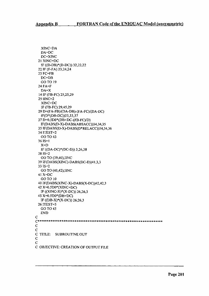
Appendix B FORTRAN Code of the UNIOUAC Modes (unsymmetric)
XINC=DADA=DCDC=XINC
21 XINC=DCIF ((DDB)*(DDC)) 32,22,22
22 IF (F-FA) 23,24,2423 FC=FB
DC=DBGO TO 19
24 FA=FDA=X
14 IF (FB-FC) 25,25,2925 1Th4C=2
XrNC=DCIF (FB-FC) 29,45,29
29 D=(FA-FB)/(DA-DB)-(FA-FC)/(DA-DC)IF(D*(DBDC))33 ,33 ,37
37 D=0.5D0(DB+DC-(FB-FC)/D)IF(DABS(D-X)-DABS(ABSACC))34,34,35
35 IF(DABS(DX)DABS(D*RELACC))34,34,3634 ITEST=2
GO 104336 IS=1
X=DIF ((DADC)*(DCD)) 3,26,38
38 IS=2GO TO (39,40),HNC
39 IF(DABS(XINC)-DABS(DC-D))4 1,3,333 IS=2
GO TO (41,42),IINC41 X=DC
GO TO 1040 IF(DABS(XINC-X)-DABS(X-DC))42,42,342 X=0.5DOt(XINC±DC)
IF ((XINCX)*(XDC)) 26,26,345 X=0.5D0(DB+DC)
IF ((DBX)*(XDC)) 26,26,326 ITEST=3
GO TO 43END
CC* * * * * * * * * * * * * * * * * * * * * * * * * * * * * * * * * * * * * * * * * * * * * * * * * * * * * * * * * * * * * * * * * * * *
CCC TITLE: SUBROUTINE OUTCCC OBJECTIVE: CREATION OF OUTPUT FILE
Page 201

Appendix B FORTRAN Code of the UNIOUAC Model (unsymmetric)
CCC********************************************************************
CSUBROUTINE OUT(NEXP)
CIMPLICIT REAL*8(AH2OZ)
CCOMMON / COMW/ COMW (12)COMMON / CORQ/ COR (12), COQ (12)COMMON / U! U(12,12)COMMON! XEX! XPREX(1000), XWAEX(1000)COMMON! GAMPR/ GAMPR(1000)COMMON/ GAMMA! GAMMA(12,1000)COMMON! TEMP/ TEMPEX(1000)COMMON! ERROR' DEL 1(1 000),DEL2( 1 000),DEL3( 1 000),SSD, RMSDCOMMON! GAMMI GAMCT( 12,1000), GAMRS( 12,1000)
CWRITE(40, 1000)
1000 FORMAT('ACTIVITY COEFFICIENT MODEL',!!!)C
WRITE(40,1 100)1100 FORMAT(!,'COMPONENT DATAV/,'NO.',4(2X),'MW',4(2X),'R',4(2X)
* ,'Q'/f)DO 100 1=1,12
WRITE(40, 1200) I,COMW(I),COR(I),COQ(I)100 CONTINUE1200 FORMAT(14,3(F 12.4))C
WRITE(40, 1500)1500 FORMAT(!/!,'UNIQUAC PARAMETERS',!/,'U(I,J)',t/)
DO 200 1=1,12WRITE(40, 1600) I,(U(I,J),J= 1,12)
200 CONTINUE1600 FORMAT(12, 12(F 12.4))C
WRITE(40, 1700)1700 FORMAT(///,'ACTIVITY COEFFICIENT RESULTS',!!,
* 'CAL',4(2X),'EXP',4(2X),'DELT,4(2X),'d X/X'!/)DO 300 I=I,NEXP
WRITE(40, 1800) GAMMA(4,I),GAMPR(1),DEL I (I),DEL2(I)300 CONTINUE1800 FORMAT(4(D 12.4))C
WRITE(40, 1900)1900 FORMAT(/,'ERRORS',//,'SSD',4(2X),'RMSD',/,)
WRITE(40,2000) SSD,RMSD2000 FORMAT(2(D 12.4))
Page 202

Appendix B FORTRAN Code of the UNIQUAC Model (unsymmetric)
CWRITE(40,2500)
2500 FORMAT(///,'GAMMA CAL.',!!,* 'LN CT',4(2X),'LN RS',4(2X),'GAMMA'!/)DO 500 J=l,NEXP
C DO 500 1-1,4WRITE(40,2600) J,4,GAMCT(4,J),GAMRS(4,J),GAMMA(4,J)
500 CONTINUE2600 FORMAT(2(12),3(D 12.4))C
WRITE(40,2700)2700 FORMAT(!/!,'GAMMA CAL.',!!,'H2O',4(2X),'PROT.',4(2X)//)
DO 800 J=1,NEXPWRITE(40,2800) J,GAMMA(1 ,J),GAMMA(4,J)
800 CONTINUE2800 FORMAT(1(12),2(D 12.4))C
WRITE(40,2 900)2900 FORMAT(/II,'EXP. DATA',//,'TEMP.',4(2X),
* 'X H2O',4(2X),'X PROT.',4(2X),'GAMMA PROT.'!!)DO 900 J=1,NEXP
WRITE(40,3000) J,TEMPEX(J),XWAEX(J),XPREX(J),GAMPR(J)900 CONTINUE3000 FORMAT(1(12),4(D 12.4))
RETURNEND
CC******************************************************************
CCC TiTLE: SUBROUTINE PACTCALCCC OBJECTIVE: CALCULATION OF ACTIVITY COEFFICIENTS ANDC OBJECTIVE FUNCTIONCCC******************************************************************
CSUBROUTINE PACTCAL(N,F,X)
CIMPLICIT REAL*8(AH2OZ)
CCOMMON! NEXPI NEXPCOMMON! CORQ/ COR(12), COQ(12)COMMON! EST! IUEST(12,12)COMMON! UI U(12, 12)
C
Page 203

C
C
C
Appendix B FORTRAN Code of the UNIOUAC Model (unsymmetric)
DIMENSION F(2000), X(40)C
L=ODO 100 K=1,12
DO 100 KK=K,12IF (IUEST(K,KK).NE.0) THEN
L=L+ 1U(K,KK)=X(L)
END IF100 CONTINUEC
DO 200 1=1,12DO 200 J=1,12
U(J,I)=U(I,J)200 CONTINUEC
CALL PUNIQUAC(NEXP)CALL PACT(NEXP)CALL POBJ(NEXP,F)CALL OUT(NEXP)
CRETURNEND
C
CCC TITLE: SUBROUTINE PACTCCC OBJECTIVE: CALCULATION OF ACTIVITY COEFFICIENTSCC
CSUBROUTINE PACT(NEXP)
IMPLICIT REAL*8(AH2OZ)
COMMON! XEXI XPREX(1000), XWAEX(1000)COMMON! GAMPRJ GAMPR( 1000)COMMON! GAMMA! GAMMA(12,1000)COMMON! TEMP! TEMPEX(1000)COMMON! ERROR! DEL 1(1 000),DEL2( 1 000),DEL3( 1 000),SSD,RMSD
SUM1=0.D0SUM2=0.D0SIJM3=0.D0
Page 204

Appendix B FORTRAN Code of the UNIOUAC Model (unsymmetric)
SUM4=0.D0DO 100 J=1,NEXP
DELI (J)=DABS(GAMPR(J)-GAMMA(4,J))SUMI=SUMI+DELI(J)DEL2(J)-DABS((GAMPR(J)-GAMMA(4,J))!GAMPR(J))SUM2-SUM2+DEL2(J)DEL3(J)=((GAMPR(J)-GAMMA(4,J))/GAMPR(J))SUM3=SUM3+DEL3(J)SUM4=SUM4+((DEL3(J))* *2)
100 CONTINUEC
SSD=SUM4RMSD=SQRT(SSD/NEXP)
CRETURNEND
CC******************************************************************CCC TITLE: SUBROUTINE POBJCCC OBJECTIVE: CALCULATES THE OBJECTIVE FUNCTION VALUE, OBJ [-]CC
* * * * * * * * * * * * * * * * * * * * * * * * * * * * * * * * * * * * * * * * * * * * * * * * * * * * * * * * * * * * * * * * *
CSUBROUTINE POBJ(NEXP,F)
CIMPLICIT REAL*8(AH2OZ)
CCOMMON! XEX! XPREX(1000), XWAEX(1000)COMMON! GAMPR/ GAMPR(1000)COMMON! GAMMA! GAMMA(12,1000)
CDIMENSION F(2000)
CFB=0.D0
CDO 200 J=1,NEXP
FB=((GAMPR(J)-GAMMA(4,J))/GAMPR(J))F(J)=FB
200 CONTINUEC
RETURNEND
C
Page 205

C
C
Appendix B FORTRAN Code of the UNIOUAC Model (unsmmetric)
C******************************************************************CCC TITLE: SUBROUTINE PUNIQ
CCC OBJECTIVE: CALCULATION OF ACTIVITY COEFFICIENTS WITH THEC UNIQUAC MODEL (UNSYMMETRIC)CCC * * * * * * * * * * * * * * * * * * * * * * * * * * * * * * * * * * * * * * * * * * * * * * * * * * * * * * * * * * * * * * * * *
CSUBROUTINE PUNIQUAC(NEXP)
IMPLICIT REAL* 8(A-H2O-Z)
COMMON / RQ / RR(12),QQ(12)COMMON / CORQ I COR(12), COQ(12)COMMON / XTR / XTR(12)COMMON / XEX / XPREX(1000), XWAEX(1000)COMMON/PT/TCOMMON / TEMP / TEMPEX( 1000)COMMON / PM / PM(12)COMMON / COMW / COMW(12)COMMON! UI U(12,12)
CCOMMON! GAM ! GAM(12)COMMON /GCT / GCT(12)COMMON !GRS / GRS(12)COMMON / GAMLN / GAMLN(12)COMMON / GAMMLN / GAMMLN(12,1000)COMMON / GAMMA I GAMMA(12,I000)COMMON / GAMM / GAMCT(12,1000), GAMRS(12,1000)
CDO 200 1=1,12
RR(I)=COR(I)QQ(I)=COQ(I)
CPM(I)=COMW(I)
C200 CONTINUEC
DO 300 J=1,NEXPC
T=TEMPEX(J)C
XTR( 1 )=XWAEX(J)XTR(4)=XPREX(J)
Page 206

Appendix B FORTRAN Code of the UNIOUAC Model (unsymmetric)
CCALL ACTCOF
CDO 320 1=1,12
GAMMA(I,J)=GAM(1)GAMMLN(I,J)= GAMLN(I)GAMCT(I,J) GCT(I)GAMRS(I,J)-GRS(I)
320 CONTINUEC300 CONTINUEC
RETURNEND
CC********************************************************************CCC SUBROUTINE ACTCOFCCC OBJECTIVE: ThIS SUBROUTINE CALCULATES THE ACTIVITY COEFFICIENTSC USING UNIQUAC MODELCC
CSUBROUTINE ACTCOF
CIMPLICIT REAL*8(A.H2OZ)
CCOMMON / GAM / GAM(12)COMMON / GCT / GCT(12)COMMON / GRS / GRS(12)COMMON / GAMLN / GAMLN(12)
CDO 2000 1=1,12
GAM(I) = 0D0GRS(I) = 0.D0GCT(I) = 0.DO
2000 CONTINUEC
CALL GAMACTCALL GAMARSDO 1000 1=1,12
GAMLN(I)=GCT(I)-f-clRS(I)CON=GAMLN(I)IF (CON.GE.174.673D0) THEN
Page 207

Appendix B FORTRAN Code of the UNIOUAC Model (unsymmetric)
GAM(I)=7.23D75ELSE
IF (CONIE.-174.673D0) THENGAM(I)=0.0D0
ELSEGAM(I) = DEXP(CON)
ENDIFENDIF
1000 CONTINUEC
RETURNEND
CC********************************************************************CCC SUBROUTINE GAMACTCCC OBJECTIVE: THIS SUBROUTINE CALCULATES THE COMBINATORIAL TERMCCC********************************************************************C
SUBROUTINE GAMACTC
IMPLICIT REAL*8(AH2OZ)C
COMMON / XTR / XTR(12)COMMON I RQ /RR(12),QQ(12)COMMON / PTh / PH(12),Th(12),THE(12)COMMON / OCT / GCT(12)COMMON / ZCOOR / ZCOOR(12)
CSR = 0.D0SQ = 0.D0DO 1000 F=I,12
SR SR + XTR(I)*RR(I)SQ = SQ + XTR(I)*QQ(I)
1000 CONTINUEC
DO 1010 1=1,12PH(I) = RR(1) SRTH(I) = QQ(I)ISQTHE(1) = XTR(I)*TH(I)
1010 CONTINUEC
DO 1020 1=1,12
Page 208

Appendix B FORTRAN Code of the UNIOUAC Model (unsymmetric)
PHI = PH(I)PHT = PHI/TH(I)GCI = DLOG(PHI) - PHIGCT(I) = Gd- 1 . D0/2 .D0*ZCOOR(I)* QQ(I)*(DLOG(PHT)PHT)
1020 CONTINUEC
DO 1030 1=1,12IF (I.EQ.1) THEN
AUX = l.D0/2.D0*ZCOOR(I)*QQ(I)GCT(I) = GCT(I) + 1 .D0 - AUX
ENDIF1030 CONTINUEC
DO 1040 1-1,12IF (I.NE.1) THEN
RAZ1 = RR(I)/RR(1)RAZ2 = QQ(1)/QQ(1)RAZ RAZI/RAZ2AUX = 1.D0/2.D0*ZCOOR(I)*QQ(I)GCT(I) = GCT(I) - DLOG(RAZ1) + RAZ1 - AUX*(RAZ - DLOG(RAZ))
ENDIF1040 CONTINUEC
RETURNEND
CC********************************************************************CCC SUBROUTINE GAMARSCCC OBJECTIVE: THIS SUBROUTINE CALCULATES THE RESIDUAL TERMCCC********************************************************************C
SUBROUTINE GAMARSC
IMPLICIT REAL* 8(A-H2O-Z)C
COMMON/PT/ICOMMON / GRS / GRS(12)COMMON / CAUX / US( I 2),S( I 2),A( I 2),C( 12,12)COMMON / RQ / RR(12),QQ(12)
CCALL GARSO1CALL GARSO3
Page 209

Appendix B FORTRAN Code of the UNIOUAC Model (unsymmetric)
CALL GARSO4C
DO 2110 1=1,12IF (I.EQ.1) THEN
GRS(I) = QQ(I)*(1 .D0 - DLOG(S(I)) -A(I))ENDIF
2110 CONTINUEC
DO 21201=1,12IF (1.NE.1) THEN
GRS(I) = QQ(I)*(DLOG(S(I))A(I)+US(I))ENDIF
2120 CONTINUEC
RETURNEND
CC********************************************************************CCC SUBROUTINE GARSOICCC OBJECTIVE: THIS SUBROUTINE CALCULATES THE RESIDUAL TERMCCC********************************************************************C
SUBROUTINE GARSO1C
IMPLICIT REAL*8(AH2OZ)C
COMMON/PT/TCOMMON / UM / UM(12,12)COMMON / U / U(12,12)COMMON / CAUX I US( 1 2),S( 12),A(1 2),C(12, 12)
CDO 1030 1=1,12
DO 1030 J=I,12UM(I,J)=U(I,J)UM(J,I)=UM(I,J)
1030 CONTINUEC
DO 2000 1=1,12IF (I.NE.1) THEN
US(I) = -(UM( I ,I)-UM(1,I))JT+DEXP(-(IJM(1, I )-UM( 1,1 ))/T)ENDIF
2000 CONTINUE
Page 210
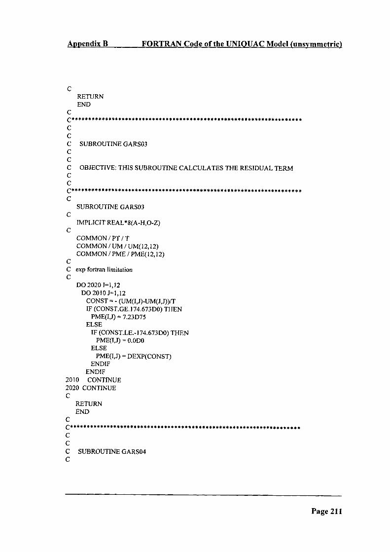
Appendix B FORTRAN Code of the UNIOUAC Model (unsymmetric)
CRETURNEND
CC********************************************************************CCC SUBROUTINE GARSO3CCC OBJECTIVE: THIS SUBROUTINE CALCULATES THE RESIDUAL TERMCCC******************************t*************************************C
SUBROUTINE GARSO3C
IMPLICIT REAL*8(AH2OZ)C
COMMON/PT/ICOMMON/UM / UM(12,12)COMMON / PME / PME(12,12)
CC exp fortran limitationC
DO 2020 1=1,12DO 2010 J=1,12
CONST = - (UM(I,J)-UM(J,J))/TIF (CONST.GE. 1 74.673D0) THEN
PME(I,J) = 7.23D75ELSE
IF (CONST.LE.-174.673D0) THENPME(I,J) = 0.ODO
ELSEPME(I,J) = DEXP(CONST)
ENDIFENDIF
2010 CONTINUE2020 CONTINUEC
RETURNEND
C
CCC SUBROUTINE GARSO4C
Page 211

Appendix B FORTRAN Code of the UNIOUAC Model (unsymmetric)
CC OBJECTIVE: THIS SUBROUTINE CALCULATES THE RESIDUAL TERMCCc********************************************************************C
SUBROUTiNE GARSO4C
IMPLICIT REAL*8(A.H2OZ)C
COMMON / PTH / PH(12),TH(12),THE(12)COMMON / PME / PME(12,12)COMMON / CAUX / US(12),S(12),A(12),C(12,12)
CDO 2040 N=1,12
SN = 0.D0DO 2030 K=1,12
SN = SN + THE(K)*PME(K,N)2030 CONTINUE
S(N) = SN2040 CONTINUEC
DO 2060 N=1,12AN = 0.D0DO 2050 K=1,12
C(N,K) = PME(N,K)/S(K)AN = AN + THE(K)*C(N,K)
2050 CONTINUEA(N) = AN
2060 CONTINUEC
RETURNEND
Page 212

Appendix C Activity Coefficient Data of Proteins
Appendix C
Activity Coefficient Data of Proteins
The activity coefficient data on the thermodynamic scale, which was determined from
osmotic pressure measurements and was used for the studies in chapter four is listed.
Page 213

Appendix C Activity Coefficient Data of Proteins
Table C. 1: Experimentally determined activity coefficients of serum albumin, S, as a
function of composition
x 7x
2.8367E-06 1.04953.9399E-06 1.0817
3.9924E-06 1.0834
4.2026E-06 1.0905
4.2551E-06 1.0924
4.9643E-06 1.1189
5.1744E-06 1.1275
5.2270E-06 1.1297
5.2270E-06 1.1297
5.2532E-06 1.1308
5.4633E-06 1.1398
5.5421E-06 1.1433
5.8573E-06 1.15766.5140E-06 1.1902
6.6716E-06 1.1985
7.5646E-06 1.2500
7.5909E-06 1.25168.0374E-06 1.2803
8.4051E-06 1.30559.5608E-06 1.3943
9.7709E-06 1.4121
9.8760E-06 1.4213
1.0296E-05 1.45931 .0480E-05 1.4766
1.2529E-05 1.7052
1.2634E-05 1.7189
1.3238E-05 1.8016
Page 214

Appendix C Activity Coefficient Data of Proteins
Table C.2: Experimentally determined activity coefficients of a - chymotrypsin, Cl, as
a function of composition
x yx
5.7972E-07 0.9978
1.1605E-06 0.9960
2.3246E-06 0.9931
3.4935E-06 0.9915
4.6668E-06 0.99 1 1
5.8443E-06 0.9919
1.2816E-05 1.0223
1.9416E-05 1.0948
2.6157E-05 1.2223
Table C.3: Experimentally determined activity coefficients of a - chymotiypsin, C2, as
a function of composition
x yx
6.1001E-07 0.9663
1.2211E-06 0.93452.4460E-06 0.8763
3.6760E-06 0.8244
4.9106E-06 0.7783
6.1496E-06 0.7373
I .3486E-05 0.57672.0430E-05 0.51442.7523E-05 0.5 155
Page 215

Appendix C Activity Coefficient Data of Proteins
Table C.4: Experimentally determined activity coefficients of a - chymotrypsin, C3, as
a function of composition
x yx
5.9401E-07 0.9570
1.1825E-06 0.9182
2.3719E-06 0.8501
3.5695E-06 0.7934
4.7736E-06 0.7463
5.9639E-06 0.7079
1.3190E-05 0.5919
1.9982E-05 0.5909
2.6920E-05 0.6452
Table C.5: Experimentally determined activity coefficients of a - chymotrypsin, C4, as
a function of composition
x yx
5.0717E-07 0.9830
1.0074E-06 0.9666
1.9907E-06 0.93572.9882E-06 0.9060
3.9369E-06 0.8792
4.9220E-06 0.8527
Page 216

Appendix C Activity Coefficient Data of Proteins
Table C.6: Experimentally determined activity coefficients of a - chymotrypsin, C5, as
a function of composition
x
5.5252E-07 0.8983
1.0756E-06 0.8116
2.1775E-06 0.65533.2197E-06 0.53524.2532E-06 0.4379
5.3356E-06 0.3550
Table C.7: Experimentally determined activity coefficients of a - chymotrypsin, C6, as
a function of composition
x .yx
1.1054E-06 0.9623
2.1781E-06 0.9270
3.2680E-06 0.8925
4.3583E-06 0.8592
5.4490E-06 0.8272
Page 217
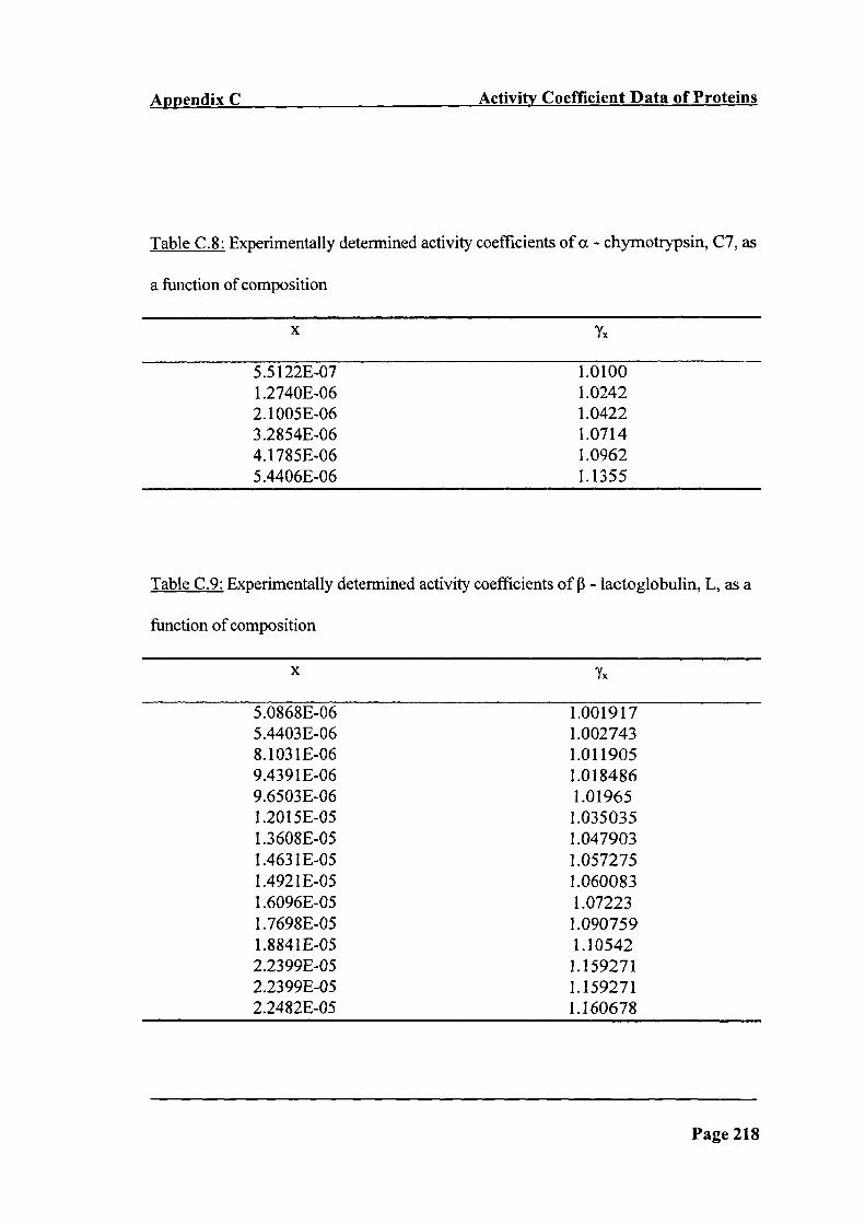
Appendix C Activity Coefficient Data of Proteins
Table C.8: Experimentally determined activity coefficients of a - chymotrypsin, C7, as
a function of composition
x .Yx
5.5122E-07 1.0100
1.2740E-06 1.0242
2.1005E-06 1.0422
3.2854E-06 1.0714
4.1785E-06 1.0962
5.4406E-06 1.1355
Table C.9: Experimentally determined activity coefficients of (3 - lactoglobulin, L, as a
function of composition
x ,yx
5.0868E-06 1.001917
5.4403E-06 1.002743
8.1031E-06 1.011905
9.4391E-06 1.018486
9.6503E-06 1.01965
1.2015E-05 1.035035
1.3608E-05 1.047903
1.4631 E-05 1.057275
1.4921E-05 1.060083
1 .6096E-05 1.07223
1 .7698E-05 1.090759
1.8841E-05 1.10542
2.2399E-05 1.159271
2.2399E-05 1.159271
2.2482E-05 1.160678
Page 218

Appendix C Activity Coefficient Data of Proteins
Table C.1 0: Experimentally determined activity coefficients of ovalbumin, 0, as a
function of composition
x Yx
9.3339E-06
1.0088
1 .0327E-05
1.0111
1 .5076E-05
1.0258
1.7803E-05
1.0371
2.0073E-05
1.0482
2.5631E-05
1.08 192.7044E-05 1.0920
Page 219
Appendix D Solubility Data of Proteins
Appendix D
Solubility Data of Proteins
The solubility data on the thermodynamic scale, which was used for the studies in
chapter five is listed.
Page 220

Appendix D Solubility Data of Proteins
Table D. 1: Experimental solubility data of lysozyme, LYS, as a function of
composition and temperature
XLYS x Temperature [K]
3.9182E-06 6.2715E-03 277.15
5.4245E-06 6.2796E-03 280.05
1.2833E-05 6.3205E-03 286.15
1.3481E-05 6.3243E-03 286.85
1.4757E-05 6.33 14E-03 287.551.6040E-05 6.3385E-03 288.15
1.7128E-05 6.3445E-03 288.65
1.8388E-05 6.3513E-03 289.15
1.9697E-05 6.3586E-03 289.75
2.1036E-05 6.3661E-03 290.4
2.3130E-05 6.3776E-03 291.15
2.5112E-05 6.3885E-03 291.85
2.8163E-05 6.4048E-03 292.553.0933E-05 6.4196E-03 293.15
3.4617E-05 6.4392E-03 293.85
4.0896E-05 6.4724E-03 294.754.5230E-05 6.4957E-03 295.654.8669E-05 6.5140E-03 296.25
5.6013E-05 6.5525E-03 297
5.9555E-05 6.5714E-03 297.6
1.2254E-06 9.4532E-03 275.551.2879E-06 9.4536E-03 276.15
1.4432E-06 9.4548E-03 277.15
1.6839E-06 9.4569E-03 278.75
1.9950E-06 9.4598E-03 280.15
2.2784E-06 9.4627E-03 281.5
2.5766E-06 9.4658E-03 282.7
3.1684E-06 9.4718E-03 284.35
3.6849E-06 9.4772E-03 285.7
4.2794E-06 9.4832E-03 286.85
4.9118E-06 9.4899E-03 288.25
5.5837E-06 9.4967E-03 289.35
Page 221

Appendix D Solubility Data of Proteins
Table Dl: con't
XLYS x Temperature IlK]
6.2234E-06 9.5031E-03 290.25
7.8269E-06 9.5187E-03 292.15
9.3617E-06 9.5334E-03 293.651.1760E-05 9.5549E-03 295.15
1.3802E-05 9.5735E-03 296.45
1.2059E-06 1.2697E-02 283.15
1.3096E-06 1.2699E-02 283.95
1.4841E-06 1.2703E-02 285.05
1.5103E-06 1.2704E-02 285.651.5251E-06 1.2705E-02 286.15
1.6188E-06 1.2707E-02 286.85
1.7514E-06 1.2710E-02 287.551.8732E-06 1.2712E-02 288.15
1.9613E-06 1.2714E-02 288.65
2.0933E-06 1.2716E-02 289.15
2.2121E-06 1.2719E-02 289.75
2.3935E-06 1.2722E-02 290.4
2.6056E-06 1.2726E-02 291.15
2.8236E-06 1.2730E-02 291.85
3.0341E-06 1.2734E-02 292.553.2691E-06 1.2738E-02 293.35
3.4466E-06 1.2742E-02 293.85
3.5524E-06 1.2744E-02 294.353.9944E-06 1.2752E-02 295.654.2793E-06 1.2757E-02 296.25
4.81 15E-06 1.2765E-02 297
5.1496E-06 1.2770E-02 297.6
2.8445E-07 1.5969E-02 275.553.1450E-07 1.5969E-02 276.153.5798E-07 l.5970E-02 277.15
4.2898E-07 1.5971E-02 278.75
4.8465E-07 1.5973E-02 280.15
5.5442E-07 1.5975E-02 281.5
6.5173E-07 l.5978E-02 282.7
Page 222

Appendix D Solubility Data of Proteins
Table D.1: con't
XLYS x Temperature [K]
7.7536E-07 1.5982E-02 284.35
9.2468E-07 1.5986E-02 285.7
1.0664E-06 1.5990E-02 286.85
1.2121E-06 1.5996E-02 288.25
1.3604E-06 1.6000E-02 289.35
1.5184E-06 1.6005E-02 290.25
1.6604E-06 1.6009E-02 291.15
2.2400E-06 1.6025E-02 293.652.7199E-06 1.6037E-02 295.15
3.2268E-06 1.6048E-02 296.45
3.7386E-06 1.6058E-02 297.351.7833E-07 2.2680E-02 275.551.9778E-07 2.2680E-02 276.15
2.2827E-07 2.2680E-02 277.15
2.5357E-07 2.2681E-02 278.75
2.9316E-07 2.2683E-02 280.15
3.1329E-07 2.2686E-02 281.5
3.7172E-07 2.2689E-02 282.7
4.3669E-07 2.2694E-02 284.35
4.9908E-07 2.2698E-02 285.7
5.7838E-07 2.2703E-02 286.85
6.42 17E-07 2.2709E-02 288.25
7.2416E-07 2.2715E-02 289.35
8.0032E-07 2.2720E-02 290.25
8.6352E-07 2.2725E-02 291.15
1.1952E-06 2.2743E-02 293.65
1.6146E-06 2.2770E-02 297.35
Page 223

Appendix D Solubility Data of Proteins
Table D.2: Experimental solubility data of concanavalin A, CON, as a function of
composition and temperature
XCON x Temperature [K]
8.1443E-07 4.6642E-03 291.157.9430E-07 4.6646E-03 292.15
7.7476E-07 4.6650E-03 293.15
7.5599E-07 4.6656E-03 294.15
7.3816E-07 4.6661E-03 295.15
7.2144E-07 4.6668E-03 296.15
7.0599E-07 4.6675E-03 297.156.9199E-07 4.6684E-03 298.15
6.8940E-07 4.6688E-03 298.55
6.7961E-07 4.6693E-03 299.15
6.6902E-07 4.6703E-03 300.15
6.6039E-07 4.6714E-03 301.15
6.5389E-07 4.6726E-03 302.156.4969E-07 4.6740E-03 303.156.4796E-07 4.6754E-03 304.15
6.4889E-07 4.6769E-03 305.156.5263E-07 4.6786E-03 306.15
6.5937E-07 4.6804E-03 307.15
6.6929E-07 4.6823E-03 308.15
6.8254E-07 4.6843E-03 309.15
6.9932E-07 4.6865E-03 310.15
7.1980E-07 4.6888E-03 311.15
7.4416E-07 4.6913E-03 312.15
7.7258E-07 4.6939E-03 313.15
7.8111E-07 4.6953E-03 313.75
8.0524E-07 4.6967E-03 314.158.4231E-07 4.6996E-03 315.15
8.8400E-07 4.7026E-03 316.15
9.3131E-07 4.7055E-03 316.95
9.3047E-07 4.7059E-03 317.15
9.8193E-07 4.7093E-03 318.15
8.5232E-08 9.5714E-03 291.15
Page 224

Appendix D Solubility Data of Proteins
Table D.2: con't
XCON Temperature [K]
8.2844E-08 9.5732E-03 292.15
8.0420E-08 9.5751E-03 293.15
7.7413E-08 9.5757E-03 293.557.8066E-08 9.5771E-03 294.15
7.5882E-08 9.5792E-03 295.157.1852E-08 9.5804E-03 295.757.3970E-08 9.5814E-03 296.15
7.2432E-08 9.5838E-03 297.157.1368E-08 9.5863E-03 298.15
7.1076E-08 9.5916E-03 300.15
7.2051E-08 9.5945E-03 301.15
7.3911E-08 9.5976E-03 302.15
8.0695E-08 9.6041E-03 304.15
8.5825E-08 9.6076E-03 305.159.2252E-08 9.61 13E-03 306.15
1.000SE-07 9.6151E-03 307.151.0941E-07 9.6191E-03 308.15
1.1172E-07 9.6228E-03 309.15
1.3301E-07 9.6276E-03 310.15
1.3129E-07 9.6283E-03 310.35
1.4748E-07 9.6322E-03 311.15
1.5576E-07 9.6338E-03 311.45
1.6388E-07 9.6369E-03 312.15
1.6709E-07 9.6375E-03 312.25
1.8231E-07 9.6418E-03 313.15
2.2569E-07 9.6523E-03 315.15
2.5085E-07 9.6578E-03 316.15
2.5403E-07 9.6597E-03 316.55
2.7848E-07 9.6636E-03 317.15
3.0867E-07 9.6695E-03 318.15
4.9661E-08 2.0374E-02 291.15
4.7435E-08 2.0378E-02 292.15
4.5204E-08 2.0382E-02 293.15
4.6658E-08 2.0384E-02 293.55
Page 225

Appendix D Soiubility Data of Proteins
Table D.2: con't
Temperature [K]
4.3033E-08 2.0387E-02 294.15
4.0985E-08 2.0391E-02 295.153.7742E-08 2.0394E-02 295.753.9124E-08 2.0397E-02 296.15
3.9734E-08 2.0397E-02 296.25
3.7514E-08 2.0402E-02 297.15
3.6219E-08 2.0407E-02 298.15
3.5303E-08 2.0413E-02 299.15
3.6793E-08 2.0418E-02 299.95
3.4830E-08 2.0420E-02 300.15
3.4865E-08 2.0426E-02 301.15
3.5473E-08 2.0433E-02 302.15
3.6716E-08 2.0440E-02 303.15
3.8662E-08 2.0447E-02 304.15
4.1373E-08 2.0455E-02 305.15
4.4915E-08 2.0463E-02 306.15
4.5853E-08 2.0468E-02 306.85
4.7849E-08 2.0469E-02 306.95
4.9354E-08 2.0471E-02 307.15
5.4755E-08 2.0479E-02 308.15
6.8704E-08 2.0497E-02 310.15
7.7384E-08 2.0507E-02 311.15
8.7290E-08 2.0517E-02 312.159.3930E-08 2.0518E-02 312.25
9.8488E-08 2.0527E-02 313.151.0650E-07 2.0533E-02 313.751.1305E-07 2.0543E-02 314.75
Page 226

Appendix E FORTRAN Code of the Solubilitv Model
Appendix E
FORTRAN Code of the Solubility Model
The FORTRAN code for the Solubility model, which was created as part of this work
for parameter determinations and solubility and activity coefficient calculations is
documented.
Page 227

C
C
Appendix E FORTRAN Code of the Solubility Model
Program routine:
C*********************************************************************
CCC AUTHOR: SABINE M. AGENACCC VERSION: 1CCC OBJECTIVE: THIS PROGRAM IS FOR PROTEiN SOLUBILITYCCC*********************************************************************C
PROGRAM PROC
IMPLICIT REAL*8 (A-H2O-Z)C
CHARACTER*30 INEXPCHARACTER3O INEXCACHARACTER*30 INPROGCHARACTER*30 [NCOMPCHARACTER*30 OUTCHARACTER*30 ourr
COMMON / IRUN/ IRUNCOMMON / NEXP/ NEXP
WRITE(* , *)'FILE NAME OF PROGRAM SPECIFIC DATA:'READ(*,'(A)') INPROGWRITE(* ,*)PILE NAME OF COMPONENT SPECIFIC DATA:'READ(*,I(A)') INCOMPWRITE(* , *)'FILE NAME FOR PROGRAM OUTPUT:'READ(*,'(A)') OUTWRJTE(* , *)IFILE NAME FOR RESULT OUTPUT:'READ(*,'(A)') OUTI'
COPEN(20,FILE=INPROG)OPEN(30,FILE=INCOMP)OPEN(40,FILE=OUT)OPEN(2 1 ,FILE=OUTF)
Page 228

Appendix E FORTRAN Code of the Solubility Model
CCALL RDINCO
CCALL RDINPR
CWRITE(* , *)'DATA WAS READ'
CIF (IRUN.EQ.0) THEN
WRITE(* ,*)'PARAMETERS WILL BE DETERMINED'C
wRITE(* ,*)'FILE NAME OF REFERENCE DATA:'READ(*,'(A)') INEXP
COPEN( I 0,FILE=INEXP)
CCALL RDINEX(NEXP)
CCALL PDET
CELSE
WRITE(* ,*)'PROTEIN SOLUBILITY WILL BE CALCULATED'C
WRITE(* ,*)'FILE NAME OF REFERENCE DATA:'C
READ(*,'(A)') INEXPC
OPEN( 1 0,FILE=INEXP)C
CALL RDINEX(NEXP)C
CALL PCALENDIF
CCLOSE( 10)CLOSE( 15)CLOSE(20)CLOSE(30)CLOSE(40)CLOSE(2 1)
CSTOPEND
CC******************************************************************CCC TITLE: SUBROUTINE RDIINCOC
Page 229

Appendix E FORTRAN Code of the Solubility Model
CC OBJECTIVE: READS IN THE COMPONENT DATA FROM FILECCC******************************************************************C
SUBROUTINE RDINCOC
IMPLICIT REAL*8 (A-H2O-Z)C
COMMON / COMW/ COMW (12)COMMON / CORQ/ COR (12), COQ (12)COMMON / Z/ Z(12)COMMON / ZCOORJ ZCOOR (12)COMMON / ABC! A,B,CCOMMON I UI U(12,12), UT(12,12)
CREAD(30, *) (COMW(I),I= 1,12)READ(30, *) (COR(I),I=1 ,12)READ(30 , *) (COQ(I),I=1 ,12)READ(30 , *) (Z(I),I=1,12)READ(30 , *) (ZCOOR(I),1= 1,12)READ(30 , *) A,B,C
CDO 100 1=1,12
READ(30 ,*) (U(I,J),J-I, 12)100 CONTiNUEC
DO 150 1=1,12READ(30, *) (UT(I,J),J=I, 12)
150 CONTINUEC
DO 200 1-1,12DO 200 J=1,12
U(J,I)=U(I,J)UT(J,I)=UT(I,J)
200 CONTINUEC
RETURNEND
CC******************************************************************CCC TITLE: SUBROUTINE RDJNPRCCC OBJECTIVE: READS PROGRAM SPECIFIC DATA FROM FILE
Page 230

Appendix E FORTRAN Code of the Solubility Model
CCC******************************************************************C
SUBROUTINE RDINPRC
IMPLICIT REAL*8 (A-.H2O-Z)C
COMMON! IRUN/ IRUNCOMMON! NEXP/ NEXPCOMMON! IABC/ IA,IB,ICCOMMON! EST/ IUEST(12,12), IUTEST(12,12)COMMON! EST1! MAXFUN, IPRll'.T,NPENCOMMON! EST2! ESCALE, EPS, SSQEPS, PMAX, WP
CREAD(20, *) IRUNREAD(20, *) NEXPREAD(20 ,*) IA,IB,IC
CDO 100 1=1,12
READ(20, *) (ILJEST(1,J),J=I, 12)100 CONTINUEC
DO 150 1=1,12READ(20 ,*) (IUTEST(I,J),J=I, 12)
150 CONTINUEC
DO 200 1=1,12DO 200 J=1,12
IUEST(J,I)=IUEST(I,J)IUTEST(J,1)=IUTEST(1,J)
200 CONTINUEC
READ(20 , *) MAXFUN, IPRINT,NPENREAD(20, *) ESCALE, EPS, SSQEPS, PMAX, WP
CRETURNEND
CCC******************************************************************
CCC TITLE: SUBROUTINE RDINEXCCC OBJECTIVE: READS EXPERIMENTAL DATA FROM FILEC
Page 231

C
C
C
C
C
C
Appendix E FORTRAN Code of the Solubility Model
CC****** ** * * * * ** ** *
CSUBROUTINE RDINEX(NEXP)
IMPLICIT REAL*8 (A-I-1,O-Z)
COMMON! TEMPt TEMPEX(1000)COMMON! XEX! XPREX(I000), XWAEX(1000), XSAEX(1000)COMMON! Z! Z( 12)COMMON! X! X(I000,12)COMMON! XUX! XUX(1000)
DO 140 J=1,NEXPREAD( I 0,*)TEMPEX(J),XSAEX(J),XWAEX(J),XPREX(J)
CZZ=Z(5)+Z(6)XUX(J)=XWAEX(J)+XPREX(J)+ZZ*XSAEX(J)X(J, 1 )=XWAEX(J)!XUX(J)X(J,4)=XPREX(J)IXUX(J)X(J,5)=Z(6)*XSAEX(J)/XUX(J)X(J,6)=Z(5)*XSAEX(J)!XUX(J)SUMX=X(J, 1 )+X(J,4)+X(J,5)+X(J,6)
C140 CONTINUEC
RETURNEND
C
CCC TITLE: SUBROUTINE PCALCCC OBJECTIVE: CALCULATES SOLUBILITY AT GIVEN TCCC* * * * * * * * * * * * * * * * * * * * * * * * * * * * * * * * * * * * * * * * * * * * * * * * * * * * * * * * * * * * * * * * * *
CSUBROUTINE PCAL
IMPLICIT REAL*8 (A-H2O-Z)
COMMON! NEXP/ NEXP
CALL PUNIQUAC(NEXP)CALL PSOL(NEXP)
Page 232

Appendix E FORTRAN Code of the Solubility Model
CALL OUT(NEXP)C
RETURNEND
C** * * * **** ***** ****** * ***** **************************** *
CCC TITLE: SUBROUTINE PDETCCC OBJECTIVE: EVALUATES THE PARAMETERS U AND UTCCC******************************************************************C
SUBROUTINE PDETC
IMPLICIT REAL*8(AFI,OZ)C
COMMON! NEXP/ NEXPCOMMON! CORQ/ COR(12), COQ(12)COMMON! ABC! A,B,CCOMMON! IABC/ IA,IB,ICCOMMON! EST! IUEST( 12,12), IUTEST(1 2,12)COMMON/U! U(12,12), UT(12,12)COMMON! EST1/ MAXFUN, IPRINT,NPENCOMMON! EST2/ ESCALE, EPS, SSQEPS, PMAX, WP
CCOMMON! FE / F(2000), E(40), X(40)
C11=0
CIF(IA.NE.0) THEN
11=11+1X(II)=A
END IFC
IF(IB.NE.0) THEN11=11+1X(H)=B
END IFC
IF(IC.NE.0) THEN11=11+1X(II)=C
END IFC
Page 233

Appendix E FORTRAN Code of the Solubility Model
DO 100 N=1,12DO 100 M=N,12
IF (IUEST(N,M).NE.0) THEN11=11+1X(II)=U(N,M)
END IF100 CONTiNUEC
DO 200 N=1,12DO 200 M=N,12
IF (IUTEST(N,M).NE.0) THEN11=11+1X(II)=UT(N,M)
END IF200 CONTINUEC
N=IIM=NEXPDO 150 1=1,40
E(I)=EPS150 CONTINUEC
CALL MINF2(M,N)C
CALL PSOLCAL(N,F,X)C
RETURNEND
CC************************************************************************CCC SUBROUTINE MINF2CCC OBJECTIVE: THIS SUBROUTINE FINDS ThE MINIMUM OF A SUM OF SQUARESC OF 'M' GIVEN FUNCTIONS OF N VARIABLES. IT USES A METhOD GIVEN INC PRESS El AL. (1986) NUMERICAL RECIPES IN FORTRAN, CAMBRIDGECCC* * * * * * * * * * * * * * * * * * * * * * * * * * * * * * * * * * * * * * * * * * * * * * * * * * * * * * * * * * * * * * * * * * * * * * * *
CSUBROUTINE MINF2(M,N)
CIMPLICIT REAL* 8(A-H2O-Z)
CCOMMON IC WORK IWORK(5 000)COMMON IICALC IICALC
Page 234

C
C
Appendix E FORTRAN Code of the Solubilitv Model
COMMON /FE /F(2000), E(40), X(40)COMMON /EST I /MAXFIJN,IPRINT,NPENCOMMON /EST2 /ESCALE,EPS,SSQEPS,PMAX,WPCOMMON /EST3 /WI(8)
ICALC=1
IER =0FFOLD = 0.ODOMPLUSN = M+NKST = N+MPLUSNNPLUS =N+1KINV = NPLUS*(MPLUSN+1)KSTORE = KINV-MPLUSN-1
CC WPJTE(6,*)I INTO CALFUN
CALL PSOLCAL(N,F,X)C
IF (ICALC.EQ.0) GO TO 999= N+N
K =NNC
DO 1 I=1,MK =K+1WORK(K) F(l)
1 CONTINUEC
IINV =2K =KST1 =1
C2 CONTINUE
X(1) = X(I) + E(I)C WRITE(6,*)' INTO CALFUN
CALL PSOLCAL(N,F,X)X(I)=X(I)-E(I)
CDO3J=l,N
K =K+1WORK(K) = 0.ODOWORK(J) = 0.ODO
3 CONTINUEC
SUM = O.ODOKK =NND04 J=1,M
KK =KK+IF(J) = F(J)-WORK(KK)
Page 235

ppendix E FORTRAN Code of the Solubilitv Model
SUM = SUM+F(J)*F(J)4 CONTINUEC
IF (SUM) 5,5,65 CONTINUE
WRITE(6,7) IWRITE(2 1,7)1
7 FORMAT(/,1X,'MESSAGE FROM MINF2 : E(',13,')'* ,'IS UNREASONABLY SMALL')DO 8 J=1,M
NN =NN+IF(J) = WORK(NN)
8 CONTINUEGOTO 10
6 CONTINUESUM=l .ODO/DSQRT(SUM)J=K-N+IWORK(J)=E(I)* SUMDO 9 J=1,M
K =K+1WORK(K) = F(J)* SUMKK =NN+JDO 1111=1,1
KK = KK+MPLUSNWORK(II) = WORK(II)+WORK(KK)*WORK(K)CONTINUE
9 CONTINUEILESS = I-iIGAMAX = N+I-1INCINV = N-ILESSINCINP = INCINV+1IF (ILESS) 13,13,14
13 CONTINUEWORK(KINV) = 1 .ODOGOTO 15
14 CONTINUEB=1 .ODODO 16 J=NPLUS,IGAMAX
WORK(J) = 0.ODO16 CONTINUE
KK=KINVDO 17 II=1,ILESS
liP = II+NWORK(IIP) = WORK(IIP)IWORK(KK)*WORK(II)JL =11+1JLAUX = JL - ILESSIF (JLAUX) 18,18,19
18 CONTINUE
Page 236

Appendix E FORTRAN Code of the Solubility Model
DO 20 JJ-JL,ILESSKK =KK+1JJP = JJ+NWORK(HP) = WORK(HP)+WORK(KK)*WORK(JJ)WORK(JJP) WORK(JJP)+WORK(KK)WORK(II)
20 CONTINUE19 CONTINUE
B = BWORK(IL)*WORK(IIP)KK = KK+INCINP
17 CONTINUEB = 1.ODOIBKK=KINVDO 21 II=NPLUS,IGAMAX
BB = B*WORK(H)DO 22 JJ=11,IGAMAX
WORK(KK) = WORK(KK)BB*WORK(JJ)KK =KK+1
22 CONTINUEWORK(KK) = BBKK = KK+INCINV
21 CONTINUEWORK(KK) = B
15 CONTINUEGO TO (27,24),IINV
24 CONTINUE1=1+1IF (I-N) 2,2,25
25 CONTINUEIINV= IFF = 0.ODOKL =NNDO 26 I=1,M
KL =KL+1F(I) = WORK(KL)FF = FF+F(I)*F(I)
26 CONTINUEICONT=1ISS=1MC=N+lIPP=IABS(IPRINT)*(IABs(IpRINT) 1)ITC=0IPs=1IPC=0
27 CONTINUEFFD = DABS(FF-FFOLD)
C WRITE(6,*) FF,FFOLD,FFD',FF,FFOLD,FFDIF (FFD.LT.SSQEPS) IER =2FFOLD = FF
Page 237

Appendix E FORTRAN Code of the Solubilitv Model
IF (IER.EQ.2) GOTO 10IPC=IPC-IABS(IPRINT)IF (IPC) 28,29,29
28 CONTINUECALL F1TINF(X,N,FF,ITC,MC,0,IER,MAXFUN)IpC=IPP
29 CONTINUEGO TO (34,35),ICONT
35 CONTINUECHANG 1 = CHANGE - 1 .ODOIF (CHANG1GT.0.D0) GOTO 36
10 CONTINUECALL FITINF(X,N,FF,JTC,MC, 1 ,IER,MAXFUN)GOTO 999
36 CONTINUEICONT=l
34 CONTINUEITC=ITC+ IK='NKK=KSTDO 39 I=1,N
K=K+ IWORK(K)=0.ODOKK='KK+NWORK(I)=0.ODODO 40 J=1,M
KK=KK+ 1WORK(I)=WORK(I)+WORK(KK)* F(J)
40 CONTINUE39 CONTINUE
DM=0.ODOKKINVDO 41 11=1,N
IIP=II+NWORK(IIP)=WORK(IIP)+WORK(K)* WORK(II)JL=II+IIF (JL-N) 42,42,43
42 CONTINUEDO 44 JJ=JL,N
JJP=JJ+NK=K+1WORK(IIP)=WORK(ILP)+WORK(K)* WORK(JJ)WORK(JJP)=WORK(JJP)+WORK(K)* WORK(II)
44 CONTINUEK=K+1
43 CONTINUEIF(DMDABS(WORK(II)*WORK(IIP))) 45,41,41
45 CONTINUE
Page 238

Appendix E FORTRAN Code of the Solubility Model
DM=DABS(WORK(II)*WORK(IIP))KL=II
41 CONTINUEThN+MPLUSN*KLCHANGE=0.ODODO 46 I=1,N
JL=N+IWORK(I)=0.ODODO 47 J=NPLUS,NN
JL=JL+MPLUSNWORK(I)_WORK(I)+WORK(J)* WORK(JL)
47 CONTINUE11=11+1WORK(II)-WORK(JL)WORK(JL)=X(I)IF(DABS(E(I)*CHANGE)DABS(WORK(I))) 48,48,46
48 CONTINUECHANGE=DABS(WORK(I)/E(I))
46 CONTINUEDO 49 1=1,M
11=11+1JL=JL+1WORK(II)=WORK(JL)WORK(JL)=F(I)
49 CONTINUEFC=FFACC=O. 1DO/CHANGEIT=3XC=O.ODOXL=0.ODQIS=3XSTEP=-DMINI (O.5D00,ESCALE/CHANGE)IF (CFIANGE-I.D0) 50,50,51
50 CONTINUEICONT=2
51 CONTINUECALL MINLIN(IT,XC,FC,6,ACC,O. I D0,XSTEP)GO TO (52,53,53,53),IT
52 CONTINUEMC=MC+ 1IF (MC-MAXFUN) 54,54,55
55 CONTINUEIER = IISS=2GOTO 53
54 CONTINUEXL=XC-XLDO 57 J=1,N
Page 239

Appendix E FORTRAN Code of the Sotubilitv Model
X(J)=X(J)+XL*WORK(J)57 CONTINUE
XL=XCC WRITE(6,*)' INTO CALFUN'
CALL PSOLCAL(N,F,X)FC=0.OD0DO 58 J=I,M
FC_FC+F(J)*F(J)58 CONTINUE
GO TO (59,59,60),IS60 CONTINUE
K=NIF (FC-FF) 61,51,62
61 CONTINUEIS=2FMIN=FCFSEC=FFGO TO 63
62 CONTINUEISr= 1FMIN=FFFSEC=FCGO TO 63
59 CONTINUEIF (FC-FSEC) 64,51,51
64 CONTINUEK=KSTOREGO TO (75,74),IS
75 CONTINUEK=N
74 CONTINUEIF (FC-FMIN) 65,51,66
66 CONTINUEFSECFCGO TO 63
65 CONTINUEIS=3-JSFSEC=FMINFMIN=FC
63 CONTINUEDO 67 JI,N
K=K+1WORK(K)=X(J)
67 CONTINUEDO 68 J=1,M
K=K+1WORK(K)=F(J)
68 CONTINUE
Page 240

Appendix E FORTRAN Code of the Solubility Model
GO TO 5153 CONTINUE
K=KSTOREKK=NGO TO (69,70,69),IS
70 CONTINUEK=NKK=KSTORE
69 CONTINUESUM=0.ODODM-0.ODOJJ=KSTORED071 J=1,N
K=K+IKK=KK+ 1JJ=JJ+ IX(J)=WORK(K)WORK(JJ)=WORK(K)-WORK(KK)
71 CONTINUEDO 72 J=1,M
K=K+1KK=KK+1JJ=JJ+ IF(J)=WORK(K)WORK(JJ)=WORK(K)-WORK(KK)SUM=SUM+WORK(JJ)* WORK(JJ)DM=DM+F(J)* WORK(JJ)
72 CONTINUEGO TO (73,10),ISS
73 CONTINUEJ=KINVKK=NPLUS-KLDO 76 I=1,KL
K=J+KL-IJ-K+KKWORK(I)=WORK(K)WORK(K)=WORK(J- 1)
76 CONTINUEIF (KL-N) 77,78,78
77 CONTINUEKL=KL+ 1JJ=KDO 79 I=KL,N
K=K+1J=J+NPLUS-IWORK(I)=WORK(K)WORK(K)=WORK(J- 1)
79 CONTINUE
Page 241

Appendix E FORTRAN Code of the Solubility Model
WORK(JJ)=WORK(K)B=I ODO/WORK(KL-1)WORK(KL- I )=WORK(N)GO TO 88
78 CONTINUEB= I .ODO/WORK(N)
88 CONTINUEK=KINVDO 80 I=1,ILESS
BB=B* WORK(I)DO 81 J=I,ILESS
WORK(K)=WORK(K) . BB* WORK(J)K=K+1
81 CONTINUEK=K+I
80 CONTINUEIF (FMIN-FF) 82,83,83
83 CONTINUECHANGE=0.ODOGO TO 84
82 CONTINUEFF=FMINCHANGE=DABS(XC)*CHANGE
84 CONTINUEXL=-DMJFMINSUM=I .ODO/DSQRT(SUM+DM*xL)K=KSTOREDO 85 I=l,N
K=K+ IWORK(K)=SUM*WORK(K)WORK(I)=0.ODO
85 CONTINUEDO 86 I=I,M
K=K+ IWORK(K)=SUM*(WORK(K)+XL*F(I))KK=NN+IDO 87 J=I,N
KK=KK+MPLUSNWORK(J)=WORK(J)+WORK(KK)*WORK(K)
87 CONTINUE86 CONTINUE
GOTO 14999 CONTINUE
RETURNEND
CCC************************************************************************
Page 242

CC
C
Appendix E FORTRAN Code of the SoIubi1it±ModeI
CCC SUBROUTINE FITINFCCC OBJECTIVE: DOCUMENTS THE SSQ AND PARAMETERS DURING THEC DETERMINATION PROCESSCCC************************************************************************C
SUBROUTINE FITINF(X,NTPAR,SSQ,ITER,NCAL,NLAST,IER,MFUTN)IMPLICIT REAL*8 (A-H2O-Z)
DIMENSJON X(NTPAR)
IF (NLAST.EQ.1.OR.IER.EQ.2) GOTO 10WRITE(2 1,1002) ITERSSQWRITE(2 1, 103 1) NCALWRITE(2 1,1001)WRITE(2 1,1030) (I,X(I),I1 ,NTPAR)WRITE(2 1,1032)WRITE(6, 1002) ITER,SSQGOTO2O
10 CONTINUEIF (IER.EQ.1) GOTO 30WRITE(2 1,2002) ITER,SSQWRITE(2 1,1031) NCALWRITE(21,2001)WRJTE(2 1,1030) (I,X(I),I= 1 ,NTPAR)IF (IER.EQ.2) WRITE (2 1,2020)IF (IER.EQ.0) WRITE (21,2021)WRITE(6,2002) ITER,SSQWRITE(6,1031)NCALWRITE(6,200 1)WRITE(6, 1030) (I,X(I),I= I ,NTPAR)IF (IER.EQ.2) WRITE (6,2020)IF (IER.EQ.0) WRITE (6,2021)GOTO 40
30 CONTINUEWRITE(2 1,1035) MFUNWRITE(21,1002) ITER,SSQWRITE(2 1,1001)WRITE(2 1,1030) (1,X(I),I=1,NTPAR)WRITE(6,1 035) MFIJNWRITE(6,1 002) ITER,SSQWRITE(6,1001)
Page 243

Appendix E FORTRAN Code of the Solubility Model
WRITE(6, 1030) (I,X(I),I=1 ,NTPAR)40 CONTINUE
WRITE(21,1032)WRITE(6, 1032)
20 CONTINUECC FORMAT DECLA.C1002 FORMAT(/, 1X,'FOR ITERATION NUMBER ',I5,//, I X,'SSQ=,D 13.6)1001 FORMAT(//,1X,'THE ACTUAL VALUES OF THE PARAMETERS ARE :',i)1030 FORMAT(1X,'X(',12,')=',D1 3.6)1031 FORMAT(/,1X,'CALFUN HAS BEEN CALLED',15,' TIMES')1032 FORMAT(/,70('*'),/)1035 FORMAT(/,'******WARNING******',/,
* 1X,'ThE NUMBER OF CALLS TO CALFUN HAS EXCEEDE',15)2002 FORMAT(/,1X,'THE ESTIMATION HAS TERMINATED NORMALLY AFTER'
* ,15,' ITERATIONS',!!,* IX,'SSQ=',D13.6)
2001 FORMAT(//,1X,'THE FINAL VALUES OF THE PARAMETERS ARE :',l)2020 FORMAT(f/,1X,'THE DESIRED ACCURACY IN SSQ WAS ACHIEVED')2021 FORMAT(//,1X,'THE DESIRED ACCURACY IN THE PARAMETERS WAS ACHIEVED'
RETURNEND
CC************************************************************************CCC SUBROUTINE MINLJNCCC OBJECTIVE: THIS SUBROUTINE FINDS THE MINIMUM OF AF FUNCTIONC OF ONE VARIABLECCC************************************************************************C
SUBROUTINE MINLIN(ITEST,X,F,MAXFUN,ABSACC,RELACC,XSTEP)C
COMMON /AUXMIN if IS,MC,DB,FB,FA,DA,D,HNCCC MODIFICATION BY S.AGENA: AUXMIN1 AND AUXMIN2 WERE CREATED FROMC AUXMIN AS THE ALIGNEMENT CREATED A WARNING WHEN COMPLIED WITH THEC F77 (NASA, SEP. 96)C
COMMON /AUXMIN2/ FC,DC,XINCDOUBLE PRECISION ABSACC,D,DA,DB,DC,F,FA,FB,FC,RELACC,X,XINC,XSTEPGO TO (1,2,2),ITEST
Page 244

Appendix E FORTRAN Code of the Solubilitv Model
2 IS=6-ITESTITEST=1IINC=1XINC=XSTEP+XSTEPMC=IS-3IF (MC) 4,4,15
3 MC-MC+1IF (MAXFUN-MC) 12,15,15
12 ITEST=443 X=DB
F=FBIF (FB-FC) 15,15,44
44 X=DCF=FC
15 RETURN1 GO TO (5,6,7,8),ISS IS=34 DC=X
FC=FX=X+XSTEPGO TO 3
7 IF (FC-F) 9,10,1110 XX+XINC
XINC=XlNC+XINCGO TO 3
9 DB=XFBFXINC-XINCGOTO 13
11 DB=DCFBr=FCDC=XFC=F
13 X=DC+DC-DBIS=2GO TO 3
6 DA=DBDBDCFA=FBFB=FC
32 DC=XFC=FGOTO 14
5 IF (FB-FC) 16,17,1717 IF (F-FB) 18,32,3218 FA=FB
DA=DB19 FB=F
Page 245

Appendix E FORTRAN Code of the Solubility Model
DB=XGO TO 14
16 IF (FA-FC) 21,21,2020 XINC=FA
FA-FCFC=XINCXINC=DADA=DCDC=XINC
21 XINC=DCIF ((DDB)*(DDC)) 32,22,22
22 IF (F-PA) 23,24,2423 FC=FB
DC=DBGO TO 19
24 FA=FDA=X
14 IF (PB-PC) 25,25,2925 JINC=2
XINC=DCIF (FB-FC) 29,45,29
29 D-(FA-FB)/(DA-DB)-(FA-FC)/(DA-DC)IF(D (DB-DC))3 3,33,37
37 D=0.5D0*(DB+DC(FBFC)/D)IF(DABS(D-X)-DABS(ABSACC))34,34,3 5
35 IF(DABS(DX)DABS(D*RELACC))34,34,3634 ITEST=2
GO TO 4336 IS=l
X=DIF ((DADC)*(DCD)) 3,26,38
38 IS=2GO TO (39,40),IINC
39 JF(DABS(XINC)-DABS(DC-D))4 1,3,333 IS=2
GO TO (41,42),IINC41 X=DC
GO TO 1040 IP(DABS(XINC-X)-DABS(X-DC))42,42,342 X=0.5D0*(XINC+DC)
IF ((XINCX)*(XDC)) 26,26,345 X=0.5D0*(DB+DC)
IF ((DBX)*(XDC)) 26,26,326 ITEST=3
GO TO 43END
CC********$***********************************************************
Page 246

Appendix E FORTRAN Code of the Solubility Model
CCC TITLE: SUBROUTINE OUTCCC OBJECTIVE: CREATION OF OUTPUT FILECCC* * * * * * * * * * * * * * * * * * * * * * * * * * * * * * * * * * * * * * * * * * * * * * * * * * * * * * * * * * * * * * * * * * * *
CSUBROUTINE OUT(NEXP)
CIMPLICIT REAL*8(AH2OZ)
CCOMMON I COMWI COMW (12)COMMON / CORQ/ COR (12), COQ (12)COMMON / UI U(12,12), UT(12,12)COMMON/ XEX/ XPREX(I000), XWAEX(1000), XSAEX(1000)COMMON! XI X( 1000,12)COMMON! SOL! SOLPR(1000)COMMON! GAMMA! GAMMA(12,1000)COMMON! TEMP! TEMPEX(1000)COMMON! ERROR! DEL 1(1 000),DEL2( 1000),DEL3( 1 000),SSD, RMSDCOMMON! GAMMI GAMCT( 12,1000), GAMRS( 12,1000)
CWRITE(40, 1000)
1000 FORMAT('SOLUBILITY MODEL',!!!)C
WRITE(40,1 100)1100 FORMAT(/,'COMPONENT DATA',//,'NO.',4(2X),'MW',4(2X),'R',4(2x)
*
DO 100 1=1,12WRITE(40, 1200) I,COMW(I),COR(I),COQ(I)
100 CONTINUE1200 FORMAT(14,3(F12 4))C
WRITE(40, 1500)1500 FORMAT(!!/,'UNIQIJAC PARAMETERS',!!,'U(I,J)',/f)
DO 200 1=1,12WRITE(40, 1600) I,(U(I,J),J= 1,12)
200 CONTINUE1600 FORMAT(12,12(F12.4))C
WRITE(40,3500)
3500 FORMAT(!//,'UNIQUAC PARAMETERS', !,'UT(I,J)',//)DO 3200 1=1,12
WRITE(40,3 600) I,(UT(I,J),J= 1,12)3200 CONTINUE
Page 247

Appendix E FORTRAN Code of the Solubility Model
3600 FORMAT(12,12(F12.4))C
WRITE(40, 1700)1700 FORMAT(///,'SOLUBILITY RESULTSY/,
* 'CAL',4(2X),'EXP',4(2X),DELT,4(2x),d X/X'//)DO 300 I=1,NEXP
WRITE(40, 1800) SOLPR(I),XPREX(1),DEL 1 (I),DEL2(I)300 CONTINUE1800 FORMAT(4(D 12.4))C
WRTTE(40, 1900)1900 FORMAT(/,'ERRORS',II,'SSD',4(2X),'RMSJY,/,)
WRITE(40,2000) SSD,RMSD2000 FORMAT(2(D12.4))C
WRITE(40,2500)2500 FORMAT(I/I,'PROTEIN GAMMA CAL.',//,
* 'LN CT,4(2X),'LN RS',4(2X),'GAMMA'//)DO 500 J=1,NEXP
C DO 500 1=1,4WRITE(40,2600) J,4,GAMCT(4,J),GAMRS(4,J),GAMTVIA(4,J)
500 CONTINUE2600 FORMAT(2(12),3(D1 2.4))C
WR1TE(40,2700)2700 FORMAT(///,'GAMMA CAL.',//,'H2O',4(2X),'PROT.',4(2x)f/)
DO 800 J= I ,NEXPWRITE(40,2800) J,GAMMA(1 ,J),GAMMA(4,J)
800 CONTINUE2800 FORMAT(1 (12),2(D 12.4))C
WRITE(40,2900)2900 FORMAT(//f,'EXP. DATA',/f,'TEMP.',4(2X),
* 'X H2O',4(2X),'X PROT.,4(2X),'X SALT/I)DO 900 J=1,NEXP
WRITE(40,3000) J,TEMPEX(J),XWAEX(J),XPREX(J),XSAEX(J)900 CONTINUE3000 FORMAT( 1 (12),4(D 12.4))C
RETURNEND
CC******************************************************************CCC TITLE: SUBROUTINE PSOLCALCC
Page 248

C
C
C
C
C
C
C
C
Appendix E FORTRAN Code of the Solubilit y Model
C OBJECTIVE: CALCULATION OF SOLUBILITY AND OBJECTIVE FUNCTIONCCC******************************************************************C
SUBROUTINE PSOLCAL(N,F,X)
IMPLICIT REAL*8(AH2OZ)
COMMON! NEXP! NEXPCOMMON! CORQ/ COR(12), COQ(12)COMMON! ABC! A,B,CCOMMON! IABC! IA,IB,ICCOMMONI ESTI IUEST( 12,12), IUTEST( 12,12)COMMON/ U! U(12,12), UT(12,12)
DIMENSION F(2000), X(40)
L=0
IF (IA.NE.0) THENL=L+IA=X(L)
END IF
IF (IB.NE.0) THENL=L+IB=X(L)
END IF
IF (IC.NE.0) THENL=L+IC=X(L)
END IF
DO 100 K=1,12DO 100 KK=K,12
IF (IUEST(K,KK).NE.0) ThENL=L+1U(K,KK)=X(L)
END IF100 CONTINUEC
DO 200 K=1,12DO 200 KK=K,12
IF (IUTEST(K,KK).NE.0) THENL=L+1UT(K,KK)=X(L)
Page 249

C
C
C
C
Appendix E FORTRAN Code of the Solubility Model
END IF200 CONTINUEC
DO 300 1=1,12DO 300 J=1,12
U(J,I)=U(I,J)UT(J,I)=UT(I,J)
300 CONTINUEC
CALL PUNIQUAC(NEXP)CALL PSOL(NEXP)CALL POBJ(NEXP,F)CALL OUT(NEXP)
CRETURNEND
CC * * * * * * * * * * * * * * * * * * * * * * * * * * * * * * * * * * * * * * * * * * * * * * * * * * * * * * * * * * * * * * * * *
CCC TITLE: SUBROUTINE PSOLCCC OBJECTIVE: CALCULATION OF SOLUBILITYCCC******************************************************************C
SUBROUTINE PSOL(NEXP)
IMPLICIT REAL*8(AH2OZ)
COMMON! ABC! A,B,CCOMMON! SOL! SOLPR(1000)COMMON! XEX/ XPREX(1000), XWAEX(1000), XSAEX(1000)COMMON! XUX/ XUX(I000)COMMON/ GAMMA! GAMMA(12,I000)COMMON! TEMP! TEMPEX(1000)COMMON/ ERROR' DELI (1 000),DEL2( I 000),DEL3( I 000),SSD,RMSD
SUM 1 =0.D0SUM2=0.D0SUM3=0.D0SUM4-0.D0
DO 100 J= 1 ,NEXPs=0S=DEXP(A+(B/TEMPEX(J)).1C*(DLOG(TEMPEX(J))))
Page 250

Appendix E FORTRAN Code of the Solubilitv Model
SOLPR(J)_XUX(J)*S/GAMMA(4,J)
CDELI (J)=DABS(XPREX(J)-SOLPR(J))SUM I =SUM I +DEL I (J)DEL2(J)=DABS((XPREX(J)-SOLPR(J))/XPREX(J))SUM2=SUM2+DEL2(J)DEL3(J)=((XPREX(J)-SOLPR(J))/XPREX(J))SUM3=SUM3+DEL3(J)SIJM4=SUM4+((DEL3(J))* *2)
100 CONTINUEC
SSD-SUM4RMSD=SQRT(SSD/NEXP)
CRETURNEND
CC******************************************************************CCC TITLE: SUBROUTINE POBJCCC OBJECTIVE: CALCULATES THE OBJECTIVE FUNCTION VALUE, OBJ [-1CCC******************************************************************C
SUBROUTINE POBJ(NEXP,F)C
IMPLICIT REAL*8(AH2OZ)C
COMMON! XEXI XPREX( 1000), XWAEX( 1000), XSAEX( 1000)COMMON! SOL/ SOLPR(1000)
CDIMENSION F(2000)
CFB=0.D0
CDO 200 J=I,NEXP
FB=((XPREX(J)-SOLPR(J))!XPREX(J))F(J)=FB
200 CONTINUEC
RETURNEND
CC******************************************************************
Page 251

C
C
C
Appendix E FORTRAN Code of the Solubility Model
CCC TITLE: SUBROUTINE PUNIQUACCCC OBJECTIVE: CALCULATION OF ACTIVITY COEFFICIENTS WITH THEC UNIQUAC MODEL (UNSYMMETRIC)CCC******************************************************************C
SUBROUTINE PUNIQUAC(NEXP)
IMPLICIT REAL*8(AH2OZ)
COMMON / RQ / RR(12),QQ(12)COMMON / CORQ I COR(12), COQ(12)COMMON I XTR I XTR(I2)COMMON / X / X(I000,12)COMMON / PT / TCOMMON / TEMP / TEMPEX(1000)COMMON / PM / PM(12)COMMON / COMW / COMW(12)COMMON / U / U(12,12),UT(12,12)
COMMON / GAM / GAM(12)COMMON /GCT / GCT(12)COMMON /GRS / GRS(12)COMMON I GAMLN / GAMLN(12)COMMON / GAMMLN / GAMMLN(12,1000)COMMON / GAMMA / GAMMA(12,1000)COMMON / GAMM / GAMCT(12,1000), GAMRS(12,1000)
CDO 200 1=1,12
RR(I)=COR(I)QQ(I)=COQ(I)
C
PM(I)=COMW(I)C200 CONTINUEC
DO 300 J=1,NEXPC
T=TEMPEX(J)C
XTR(1)=X(J,1)XTR(4)=X(J,4)XTR(5)=X(J,5)
Page 252

Appendix E FORTRAN Code of the Solubilitv Model
XTR(6)=X(J,6)C
CALL ACTCOFC
DO 320 1=1,12GAMMA(I,J)=GAM(I)GAMMLN(I,J)= GAMLN(I)GAMCT(I,J)=GCT(I)GAMRS(I,J)=GRS(I)
320 CONTINUEC300 CONTINUEC
RETURNEND
CC********************************************************************CCC SUBROUTINE ACTCOFCCC OBJECTIVE: THIS SUBROUTINE CALCULATES THE ACTIVITY COEFFICIENTSC USING UNIQUAC MODELCC
CSUBROUTINE ACTCOF
CIMPLICIT REAL* 8(A-H2O-Z)
CCOMMON / GAM / GAM(12)COMMON / GCT / GCT(12)COMMON / GRS / GRS(12)COMMON / GAMLN / GAMLN(12)
CDO 2000 1=1,12
GAM(I) = 0.D0GRS(I) = 0.DOGCT(I) = 0.D0
2000 CONTINUEC
CALL GAMACTCALL GAMARSDO 1000 1=1,12
GAMLN(I)=GCT(I)+GRS(I)CON=GAMLN(I)
Page 253

Appendix E FORTRAN Code of the Solubility Model
IF (CON.GE.174.673D0) THENGAM(1)=7.23D75
ELSEIF (CON.LE...174.673D0) THEN
GAM(I)=0.ODOELSE
GAM(I) = DEXP(CON)ENDIF
ENDIF1000 CONTINUEC
RETURNEND
CC* * * * * * * * * * * * * * * * * * * * * * * * * * * * * * * * * * * * * * * * * * * * * * * * * * * * * * * * * * * * * * * * * * * *
CCC SUBROUTINE GAMACTCCC OBJECTIVE: THIS SUBROUTINE CALCULATES THE COMBINATORIAL TERMCCC******** *************************** ** *** * ****** *************** * **** *
CSUBROUTINE GAMACT
CIMPLICIT REAL*8(AH2OZ)
CCOMMON / XTR / XTR(12)COMMON / RQ /RR(12),QQ(12)COMMON / PTH / PH(I2),TH(12),THE(12)COMMON / GCT / GCT(12)COMMON I ZCOOR / ZCOOR( 12)
CSR = ODOSQ = 0.D0DO 1000 1=1,12
SR = SR + XTR(I)*RR(I)SQ = SQ + XTR(I)*QQ(I)
1000 CONTINUEC
DO 1010 1=1,12PH(I) = RR(I)/SRTH(I) = QQ(1) SQTHE(I) = XTR(I)*TII(I)
1010 CONTINUEC
Page 254

Appendix E FORTRAN Code of the Solubility Model
DO 1020 1=1,12PHI = PH(I)PHI = PHIITH(I)GCI = DLOG(PHI) - PHIGCT(I) = Gd- I .DO/2.D0*ZCOOR(I)*QQ(I)*(DLOG(PHT)PHT)
1020 CONTINUEC
DO 1030 1=1,12IF (I.EQ.1) ThEN
AUX = I .D0/2.DO*ZCOOR(I)*QQ(l)GCT(I) = GCT(I) + 1 .D0 - AUX
ENDIF1030 CONTINUEC
DO 1040 1=1,12IF (I.NE.1) THEN
RAZ1 = RR(I)IRR(1)RAZ2 = QQ(1)/QQ(1)RAZ = RAZ IIRAZ2AUX = I.DO/2.D0*ZCOOR(I)*QQ(I)GCT(I) = GCT(I) - DLOG(RAZ1) + RAZI - AUX*(RAZ - DLOG(RAZ))
ENDIF1040 CONTINUEC
RETURNEND
C
CCC SUBROUTINE GAMARSCCC OBJECTIVE: THIS SUBROUTINE CALCULATES THE RESIDUAL TERMCCC********************************************************************C
SUBROUTINE GAMARSC
IMPLICIT REAL*8(AH2OZ)C
COMMON / PT ITCOMMON / GRS / GRS(12)COMMON / CAUX / US( 1 2),S( 12),A( I 2),C( 12,12)COMMON / RQ /RR(12),QQ(12)
CCALL GARSO1
Page 255

Appendix E FORTRAN Code of the Solubility Model
CALL GARSO3CALL GARSO4
CDO 2110 1=1,12
IF (I.EQ.1) THENGRS(I) = QQ(I)*(1 .D0 - DLOG(S(I)) -A(I))
EN DIP2110 CONTINUEC
DO 2120 1=1,12IF (LNE.1) THEN
GRS(I) = QQ(I)*(DLOG(S(I))A(I)+US(I))ENDIF
2120 CONTINUEC
RETURNEND
CC********************************************************************CCC SUBROUTINE GARSOICCC OBJECTIVE: THIS SUBROUTINE CALCULATES THE RESIDUAL TERMCCC* ** * * * ** ******** ***************************************** ****
CSUBROUTINE GARSO1
CIMPLICIT REAL*8(AH2OZ)
CCOMMON/PT/TCOMMON / UM / UM(12,12)COMMON / U / U(12,12),UT(12,12)COMMON / CAUX / US(12),S(12),A(12),C(12,12)
CDO 1030 1=1,12
DO 1030 J=I,12UM(I,J)=U(I,J)+(UT(I,J)*(T300))UM(J,I)=UM(I,J)
1030 CONTINUEC
DO 2000 1=1,12IF (I.NE.1) THEN
US(I) = -(UIvl( I ,I)-L.JlvI(I,I))/T+DEXP(-(UM(I, 1 )-UM( 1,1 ))/T)ENDIP
Page 256

Appendix E FORTRAN Code of the Solubility Model
2000 CONTINUEC
RETURNEND
CC**********************$*********************************************
CCC SUBROUTINE GARSO3CCC OBJECTIVE: THIS SUBROUTINE CALCULATES THE RESIDUAL TERMCCC********************************************************************C
SUBROUTINE GARSO3C
IMPLICIT REAL*8(A..H2OZ)C
COMMON/PT/ICOMMON / UM / UM(12,12)COMMON / PME / PME(12,12)
CC exp fortran limitationC
DO 2020 1=1,12DO 2010 J=1,12
CONST = - (UM(I,J)-UM(J,J))/TIF (CONST.GE.174.673D0) THEN
PME(I,J) = 7.23D75ELSE
IF (CONST.LE.-174.673D0) THENPME(I,J) = 0.ODO
ELSEPME(1,J) = DEXP(CONST)
ENDIFENDIF
2010 CONTINUE2020 CONTINUEC
RETURNEND
C
CCC SUBROUTINE GARSO4
Page 257

Appendix E FORTRAN Code of the Solubility Model
CCC OBJECTIVE: THIS SUBROUTINE CALCULATES THE RESIDUAL TERMCCC********************************************************************
CSUBROUTINE GARSO4
CIMPLICIT REAL*8(AH2OZ)
CCOMMON / PTH / PH(12),TH(12),THE(12)COMMON / PME I PME( 12,12)COMMON / CAUX / US(12),S(12),A(12),C(12,12)
CDO 2040 N=1,12
SN = 0.D0DO 2030 Kr=1,12
SN = SN + THE(K)*PME(K,N)2030 CONTINUE
S(N) = SN2040 CONTINUEC
DO 2060 N=I,12AN = O.D0DO 2050 K=1,12
C(N,K) = PME(N,K)/S(K)AN = AN + ThE(K)*C(N,K)
2050 CONTINUEA(N)=AN
2060 CONTINUEC
RETURNEND
Page 258

References
References
Abrams, D.S., Prausnitz, J.M. (1975) Statistical thermodynamics of liquid mixtures: a
new expression for the excess Gibbs energy of partly or completely miscible systems.
AIChE J., 21(1), 116.
Agena, S.M., Wai, P. and Bogle, LD.L. (1996) Property prediction methods for
biochemical synthesis and design. Research Event of the Institution of Chemical
Engineers, Leeds, UK
Agena, S.M., Pusey, M.L. and Bogle, I.D.L. (1997a) Solid - liquid equilibrium model
for biopolymers. Conference of the American Institute of Chemical Engineers,
Spring Meeting, Houston, USA
Agena, S.M., Bogle, I.D.L. and Pessoa, F.L.P. (1997b) An activity coefficient model
for proteins. Biotech. Bioeng., 55 (1) 65 - 71
Page 259

References
Agena S.M., Pusey M., Bogle I.D.L. (1998a) A model for protein solubility.
Submitted.
Agena S.M., Bogle LD.L., Pusey M. (1998b) Studies of protein solution properties
using osmotic pressure measurements. Submitted.
Asenjo, J.A. (ed. Plye, D.L.) (1990) Separations for biotechnology. Elsevier.
Bailey, J.E., 011is, D.F. (1986). Biochemical engineering fundamentals. McGraw-
Hill.
Bamicki S.D., James R.F. (1990) Separation system synthesis: a knowledge-based
approach. 1. Liquid mixture separation. md. Eng. Chem. Res., 29,421.
Blundell T.L., Johnson L.N. (1976) Protein crystallography. Academic Press.
Bogle, I., Wai, P., Agena, S., Gani, R., Bagherpour, K., Nielsen, J., Carisen, M.,
Aracil, J., Martinez, M., Bautista, F., Soriano, R., Coteron, A., Norodoslawsky, M.,
Altenburger, J., Schichi, M. and I-Ialasz, L. (1996) Process synthesis, design and
simulation of integrated biochemical processes. Fifth World Congress of Chemical
Page 260

References
Engineering, San Diego, USA
Bondi, A. (1968) Physical properties of molecular cr ystals, liquids and glasses. John
Wiley & Sons.
Bonnerjea, J., Oh, S., bare, M., Dunnill, P. (1986) Protein purification: the right step
at the right time. Bio/Tech., 4, 954.
Burgess, R.R. (eds. Oxender, D.L., Fox, C.F.) (1988) Protein engineering. Alan R Liss,
Inc.
Cacioppo, E., Pursey, M.L. (1991) The solubility of the tetragonal form of hen egg
white lysozyme from pH 4.0 to 5.4. J. Crystal Growth, 114, 286.
Cacioppo, E., Pusey, M.L. (1992) The effect of acid treatment and calcium ions on
the solubility of concanavalin A. J. Crystal Growth, 122, 208.
Carbonnaux C., Ries-Kautt M., Ducruix A. (1995) Relative effectiveness of various
anions on the solubility of acidic hypoderma lineatum collagenase at pH 7.2. Protein
Science, 4, 2123.
Page 261

References
Carter D.C., He X.-M., Munson S.H., Twigg RD., Gemert K.M., Broom M.B.,
Miller T.Y. (1989) Three-dimensional structure of human serum albumin. Science,
244, 1195.
Chiew, Y.C., Kuelmer, D., Blanch, H.W., Prausnitz, J.M. (1995) Molecular
thermodynamics for salt - induced protein precipitation. AIChE J., 41, 2150.
Chothia, C. (1975) Structural invariants in protein folding. Nature, 254, 304.
Christensen, L.K. (1952) Denaturation and enzymatic hydrolysis of lactoglobulin.
Comp.-rend. Lab. Carlsberg, 28, 37.
Cohn, E.J (1925) The physical chemistry of the proteins. Physiol. Rev., 5, 349.
Cohn, E.J., Edsall, J.T. (1943) Proteins, amino acids and peptides. Reinhold
Publishing Corporation.
Constantinou L., Gani R. (1994) A new group-contribution method for the estimation
of properties of pure compounds. AIChE J., 40, 1697.
Page 262

References
Coutinho J.A.P., Andersen S.I., Stenby E.H. (1994) Evaluation of activity coefficient
models in prediction of alkane solid-liquid equilibria. IVC-SEP report, Department of
Chemical Engineering, Technical University of Denmark (DTU), Lyngby, Denmark.
Cranfield, R.E., Liu, A.K. (1965) The disulfide bonds of egg white lysozyme. J. Bio.
Chem., 240 (5), 1997.
Creighton, T.E. (1984) Proteins: structures and molecular properties. W.H. Freeman
and Company.
Debye P., Hückel E. (1923) Zur Theory der Elektrolyte. I. Gefrierpunktserniedrigung
und verwandte Erscheinungen. Phy. Zeitsch., 24(9), 185.
Debye P. (1927) Das electrische lonenfeld und das Aussaizen. Z. physik. Chem., 130,
56.
Deschamps J.R., Miller C.E., Ward KB. (1995) Rapid purification of recombinant
green fluorescent protein using the hydrophobic properties of an HPLC size - exclusion
column. Protein Expres. Purif., 6, 555.
Page 263

References
Dixon M., Webb E.C. (1961) Enzyme fractionation by salting out: A theoretical note.
Advan. Protein Chem., 16, 197.
Ducruix, A., Giege, R. (1992) Crystallization of nucleic acids and proteins. A
practical approach. IRL Press.
Edsall, J.T., Wyman, J. (1958) Biophysical chemistry. Academic Press Inc.
Elbro H.S., Fredenslund Aa., Rasmussen P. (1991) Group contribution method for the
prediction of liquid densities as a function of temperature of solvents, oligomers, and
polymers. md. Eng. Chem. Res., 30(12), 2577.
Elmore D.T. (1968) Peptides and proteins. Cambridge University Press.
Ewing, F., Forsythe, E., Pusey, M. (1994) Orthorombic lysozyme solubility. Acta
Cryst., D50, 424.
Forsythe, E.L., Pusey, M.L. (1996) The effects of acetate buffer concentration on
lysozyme solubility. J. Crystal Growth, 168, 112.
Page 264

References
Foster P.R., Dunnill P., Lilly M.D. (1971) Salting-out of enzymes with ammonium
sulfate. Biotech. Bioeng., XIII, 713.
Fraaije, J.G.E.M., Norde, W., Lykiema, J. (1991) Interfacial thermodynamics of
protein adsorption, ion co - adsorption and ion binding in solution. II. Model
interpretation of ion exchange in lysozyme chromatography. Biophy. Chem., 40, 317.
Fredenslund, Aa., Jones, R.L., Prausnitz, J.M. (1975) Group-contribution estimation of
activity coefficients in nonideal liquid mixtures. AIChE J., 21, 1086.
Fredenslund Aa. (1989) UNIFAC and related group contribution models for phase
equilibria. Fluid Phase Equil., 52, 135.
Freifelder D. (1986) Molecular biology. Jones and Barlett Publishers.
Gmehling, J.G., Anderson, T.F., Prausnitz, J.M. (1978) Solid - liquid equilibria using
UNIFAC. md. Eng. Chem. Fundam., 17(4), 269.
Green A.A. (1931) Studies in the physical chemistry of the proteins. VIII. The
solubility of hemoglobin in concentrated salt solutions. A study of the salting out of
Page 265

References
proteins. J. Biol. Chem., 93, 495.
Green A.A. (1932) Studies in the physical chemistry of the proteins. X. The solubility
of hemoglobin in solutions of chlorides and sulfates of varying concentration. J. Biol.
Chem., 95, 47.
Green A.A., Hughes W.L. (1955) Protein fractionation on the basis of solubility in
aqueous solutions of salts and organic solvents. Methods in Enzymology, I, 67.
Guntelberg, A.V., Linderstrom-Lang, K. (1949) Osmotic pressure of plakalbumin
and ovalbumin solutions. Compt.-rend. Lab. Carlsberg, 27, 1.
Gupta, R.B., Heidemann, R.A. (1990) Solubility models for amino acids and antibotics.
AIChE J., 36 (3), 333.
Hansen, H.K., Rasmussen, P., Fredenslund, Aa., Schiller, M., Gmehling, J. (1991)
Vapor-liquid equilibria by UNIFAC group contribution. 5. Revision and extension. md.
Eng. Chem. Res., 30, 2352.
Haynes, C.A., Tamura, K., Korfer, I-JR., Blanch, H.W., Prausnitz, J.M. (1992)
Page 266
References
Thermodynamic properties of aqueous a-chymotrypsin solutions from membrane
osmometry measurements. J. Phys. Chem., 96, 905.
He X.-M., Carter D.C. (1992) Atomic structure and chemistry of human serum
albumin. Nature, 358, 209.
Ho, J.X., Holowachuk, E.W., Norton, E.J., Twigg, P.D., Carter, D.C. (1993) X-ray
and primary structure of horse serum albumin (Equus caballus) at 0.27-nm
resolution. Eur. J. Biochem., 215, 205.
Hofmeister, F. (1888) Zur Lebre von der Wirkung der Saize. Arch. Exp. Pathol.
PharmakoL, 24,247.
Hoshino D., Nagahama K., Hirata M. (1982) Prediction of acentric factor of alkanes by
the group contribution method. J. Chem. Eng. Japan, 15 (2), 153.
Hückel E. (1925) Zur Theorie konzentrierterer wasseriger Lösungen starker
Elektrolyte. Phy. Zeitsch., 26 (2), 93.
Israelachvili J.N. (1985) Intermolecular and surface forces. Academic Press.
Page 267

References
Jakoby, W.B. (1968) A technique for the crystallization of proteins. Analytical
Biochem., 26, 295.
Jaksland C.A., Gani R., Lien K.M. (1995) Separation process design and synthesis
based on thermodynamic insight. Chem. Eng. Science, 50 (3), 511.
Janin, J. (1976) Surface area of globular proteins. J. Mol. Biol., 105, 15.
Judge R. (1997) Personal communication.
Kikic I., Alessi P., Rasmussen P., Fredenslund Aa. (1980) On the combinatorial part of
the UNIFAC and UNIQUAC models. Can. J. Chem. Eng., 58, 253.
Klincewicz K.M., Reid R.C. (1984) Estimation of critical properties with group
contribution methods. AIChE J., 30 (1), 137.
Kontogeorgis, G.M., Nikolopoulos, G.I., Fredenslund, Aa., Tassios, D.P. (1997)
Improved models for the prediction of activity coefficients in nearly athermal mixtures.
Part II. A theoretically-based GE-model based on the van der Waals partition function.
Fluid Phase Equil., 127, 103.
Page 268

References
Kuehner, D.E., Blanch, H.W., Prausnitz, J.M. (1996) Salt - induced protein
precipitation; Phase equilibria from an equation of state. Fluid Phase Equil., 116,
140.
Laidler, K.J., Meiser, J.H. (1982) Physical chemistry. The BenjaminlCummings
Publishing Company, Inc.
Larsen, B.L., Rasmussen, P., Fredenslund, Aa. (1987) A modified UNIFAC group-
contribution model for prediction of phase equilibria and heat of mixing. md. Eng.
Chem. Res., 26,2274.
Lehninger, A.L. (1982) Principles of biochemistry. Worth Publishers, Inc.
Lydersen A.L. (1955) Estimation on critical properties of organic compounds by the
method of group contribution. Report no.3, College of Engineering, University of
Wisconsin.
Lyman, W.J., Reehi, W.F., Rosenblatt, D.H. (1982) Handbook of chemical property
estimation methods. Mc Graw - Hill.
Page 269

References
Matthews, B.W., Sigler, P.B., Henderson, R., Blow, D.M. (1967) Three-dimensional
structure of tosyl - a - chymotrypsin. Nature, 214, 652.
Mavrovouniotis M.L., Bayol P., Lam T.K.M., Stephanopoulos G., Stephanopoulos G.
(1988) A group contribution method for the estimation constants for biochemical
reactions. Biotech. Techniques, 2 (1), 23-28.
Mavrovouniotis M.L. (1990) Group contributions for estimating standard Gibbs
energies of formation of biochemical compounds in aqueous solution. Biotech.
Bioeng., 36, 1070-1082.
McPherson A., Rich A. (1973) X-ray crystallographic study of the quatemary structure
of canavalin. J. Biochem., 74, 155.
McPherson A., Spencer R. (1975) Preliminary structure analysis of canavalin from Jack
Bean. Arch. Biochem. Biophys. Res. Commun., 57, 494.
McPherson A. (1982) Preparation and analysis of protein cr ystals. John Wiley & Sons.
Melander, W., Horvath, C. (1977) Salt effects on hydrophobic interactions in
Page 270

References
precipitation and chromatography of proteins: An interpretation of the lyotropic series.
Archives Biochem. Biophy., 183, 200.
Mullin J.W. (1993) Crystallization. Butterworth-Heinemann.
Nass, K.K. (1988) Representation of the solubility behavior of amino acids in water.
AIChE J., 34 (8), 1257.
Nicolaisen, H., Rasmussen, P., Sorensen, J.M. (1993) Correlation and prediction of
mineral solubilities in the reciprocal salt system (Na, K) (C1, SO 42 )-H20 AT 0-
100°C. Chem. Eng. Sci., 48 (18), 3149.
Nicolaisen, H. (1994) Phase equilibria in aqueous electrolyte solutions. Ph.D. thesis,
Department of Chemical Engineering, Technical University of Denmark (DTU),
Lyngby, Denmark.
Niktari M., Richardson P., Ravenhall P., Flanagan M.T., Molloy J., Hoare M. (1989)
The modelling and control of fractionation processes for enzyme and protein
purification. Proceedings Am. Control Conf, 3, 2436.
Page 271
References
Nisbet, A.D., Saundry, R.H., Moir, A.J.G., Fothergill, L.A., Fothergill, J.E. (1981) The
complete amino-acid sequence of hen ovalbumin. Eur. J. Biochem., 115, 335.
Pauling L.C. (1960) The nature of the chemical bond. Cornell University Press.
Peres, A.M., Macedo, E.A. (1994) Representation of solubilities of amino acids using
the UNIQUAC model for electrolytes. Chem. Eng. Science, 49 (22), 3803.
Perozzo M.A. (1997a) Personal communication.
Perozzo M.A. (1997b) X-ray crystallographic structural analysis of aequorea victoria
green fluorescent protein. Ph.D. thesis, Department of Chemistry, The Catholic
University of America, Washington, D.C., USA.
Pervaiz, S., Brew, K. (1985) Homology of - lactoglobulin, serum retinol-binding
protein, and protein HC. Science, 228, 335.
Pessoa, F.L.P., Rasmussen, P., Fredenslund, Aa. (1992) Calculation of vapor-liquid
equilibria in water - sulfuric acid - sulfate salt systems using a revised extended
UNIQUAC equation. Latin American Applied Research, 22, 195.
Page 272

References
Pinho, S.P., Silva, C.M., Macedo, E.A. (1994) Solubility of amino acids: a group-
contribution model involving phase and chemical equilibria. md. Eng. Chem. Res., 33,
1341.
Prausnitz, J.M., Lichtenthaler, R.N., Gomes de Azevedo, E. (1986) Molecular
thermodynamics of fluid-phase equilibria. Prentice-Hall.
Press, W.H., Teukolsky, S.A., Vetterling, W.T., Flannery, B.P. (1986) Numerical
recipes in Fortran. Cambridge University Press.
Przybycien, T.M., Bailey, J.E. (1989) Solubility - activity relationship in the
inorganic salt - induced precipitation of a - chymotrypsin. Enz. Microb. Teclmol., 11,
264.
Pusey, M.L., Gemert, K. (1988) A method for rapid liquid-solid phase solubility
measurements using the protein lysozyme. J. of Crystal Growth, 88, 419.
Pusey, M.L., Munson, S. (1991) Micro - apparatus for rapid determination of protein
solubilities. J. Crystal Growth, 113, 385.
Page 273

References
Pusey, M.L. (1996) Personal communication.
Pusey, M.L. (1997) Personal communication.
Reid, R.C., Prausnitz, J.M., Poling, B.E. (1987) The properties of gases & liquids.
McGraw - Hill.
Renon, H., Prausnitz, J.M. (1968) Local composition in thermodynamic excess for
liquid mixtures. AIChE J., 14 (1), 135.
Richards, F.M. (1974) The interpretation of protein structures: total volume, group
volume distributions and packing density. J. Mol. Biol., 82, 1.
Ross, P.D., Minton, A.P. (1977) Analysis of non-ideal behavior in concentrated
hemoglobin solutions. , J. Mol. Biol., 112, 437.
Roth, C.M., Neal, B.L., Lenhoff, A.M. (1996) Van der Waals interactions involving
proteins. Biophy. J., 70, 977.
Sander, B., Fredenslund, Aa., Rasmussen, P. (1986) Calculation of vapour-liquid
Page 274

References
equilibria in mixed solvent/salt systems using an extended UNIQUAC equation. Chem.
Eng. Science, 41(5), 1171.
Scopes, R. K. (1987) Protein purification. Springer Verlag.
Shih, Y.-C., Prausnitz, J. M., Blanch, H.W. (1992) Some Characteristics of protein
precipitation by salts. Biotech. Bioeng., 40, 1155.
Siirola J.J., Rudd D.F. (1971) Computer-aided synthesis of chemical process designs.
md. Eng. Chem. Fundam., 10 (3), 353.
Smith, J.M., van Ness, H.C. (1987) Introduction to chemical engineering
thermodynamics. McGraw-Hill.
Sober, H.A. (ed.) (1968) Handbook of biochemistr y. CRC Press.
Soehnel 0., Garside J. (1992) Precipitation. Butterworth-Heinemann.
Tanford, C. (1961) Physical chemistry of macromolecules. John Wiley & Sons.
Page 275

Reference
Taratuta, V.C., Holschbach, A., Thurston, G.M., Blankschtein, D., Benedek, G.B.
(1990) Liquid-liquid phase separation of aqueous lysozyme solution: effects of pH and
salt identity. J. Phy. Chem., 94(5), 2140.
Taylor, G.L. (ed. Crabbe M.J.C.) (1990) Structure prediction, enzyme biotechnology.
Ellis -1-lorwood.
Teller, D.C. (1976) Accessible area, packing volumes and interaction surfaces of
globular proteins. Nature, 260, 729.
Wai, P.P.C., Bogle I.D.L., Bagherpour K., Gani R. (1996) Process synthesis and
simulation strategies for integrated biochemical process design. Computers. Chem.
Eng., 20, S357.
Wheelwright, S.M. (1987) Designing downstream processes for large-scale protein
purification. Bio/Tech., 5, 789.
Wheelwright S.M. (1991) Protein purification. Carl Hansen Verlag.
Wills, P.R., Comper, W.D., Winzor, D.J. (1993) Thermodynamic nonideality in
Page 276

References
inacromolecular solutions: interpretation of virial coefficients. Arch. Biochem.
Biophy. 300, 206.
Wilson, G.M. (1964) Vapour-liquid equilibrium Xl. A new expression for the excess
free energy of mixing, J. Am. Chem. Soc., 86, 127.
I BI3Lt Page 277(LONDIN)