MODELLING OF SPRAY DEPOSIT - DCU HomeCHAPTER 4: MODELLING OF SPRAY DEPOSIT 4 MODELLING OF SPRAY DEPOSIT 4.1 FINITE ELEMENT ANALYSIS The finite element method is a numerical procedure,

CHAPTER 4: MODELLING OF SPRAY DEPOSIT

4 MODELLING OF SPRAY

DEPOSIT 4.1 FINITE ELEMENT ANALYSIS

The finite element method is a numerical procedure, that can be used to obtain

solutions to a large class of engineering systems, including stress analysis, heat

transfer, fluid flow and electromagnetism. In thermal spraying, finite element analysis

is used either to validate or predict experimental results, through numerical

formulation. Residual stress is a major problem in thermal spraying where high

thickness coatings are required, due to the rapid solidification and cooling of sprayed

droplets during cooling. Experimental analysis may help the researcher understand

where these stresses arise in a component, hence lead to the prevention of such

outcomes. Finite element analysis may support experimental findings and predict

results for more complex situations. In general most of the analyses of residual stress,

consist of analytical models of the behaviour of molten droplets striking the substrate

surface, similar to that detailed by Fukanuma et al. [101], nevertheless finite element

analysis similar to that shown here has also been documented [102,103]. In this

research finite element analysis of heat transfer and residual stress in the coated sample

is carried out and compared to experimental data generated during the current research.

There are many finite element method software programs available to yield various

engineering solutions, however the ANSYS finite element program was used in the

current research, as it is widely available within the university. Hence the followings

sections are specific to the ANSYS program.

The origin of the modern finite element method may be traced back to the early 1900s,

when some investigators approximated and modelled elastic continua using discrete

equivalent elastic bars. The ANSYS finite element method program was released in

________________________________________________________________________________________________ Production of Coated and Free-Standing Engineering Components Using the HVOF (High Velocity Oxy-Fuel) Process J. Stokes

91


1971 for the first time. ANSYS is a comprehensive general purpose finite element

computer program, which contains over 100,000 lines of code [104]. ANSYS is

capable of performing static, dynamic, heat transfer, fluid flow, and electromagnetism

analyses. The current version of ANSYS has multiple windows incorporating a

Graphical User Interface (GUI), pull-down menus, dialog boxes, and a tool bar. The

objective of this section is to introduce the basic concepts in finite element formulation,

including numerical formulation. The following topics are addressed:

• Engineering Problems

• Numerical Methods

• Steps in the Finite Element Method

• Numerical Formulation of systems specific to this research

• Verification of Results


92


4.2 ENGINEERING PROBLEMS

Engineering problems can be described in general as being mathematical models of

physical situations [105]. The mathematical models generally comprise of numerous

differential equations with sets of corresponding initial and boundary conditions. The

differential equations are derived by applying fundamental laws and principles of

nature to an engineering system. These equations represent the balance of mass, force,

or energy and when possible, the solution of these equations renders a detailed

behaviour of a system under a given set of conditions.

Analytical solutions show the exact behaviour of a system at any point within the

system. An analytical solution may be composed of two parts: firstly a homogenous

part and secondly a particular part. In any engineering system, there are two sets of

parameters that influence the way a system behaves. Firstly, there are those parameters

that provide information regarding the natural behaviour of a given system and always

appear in the homogeneous part of the solution. Examples of these parameters include

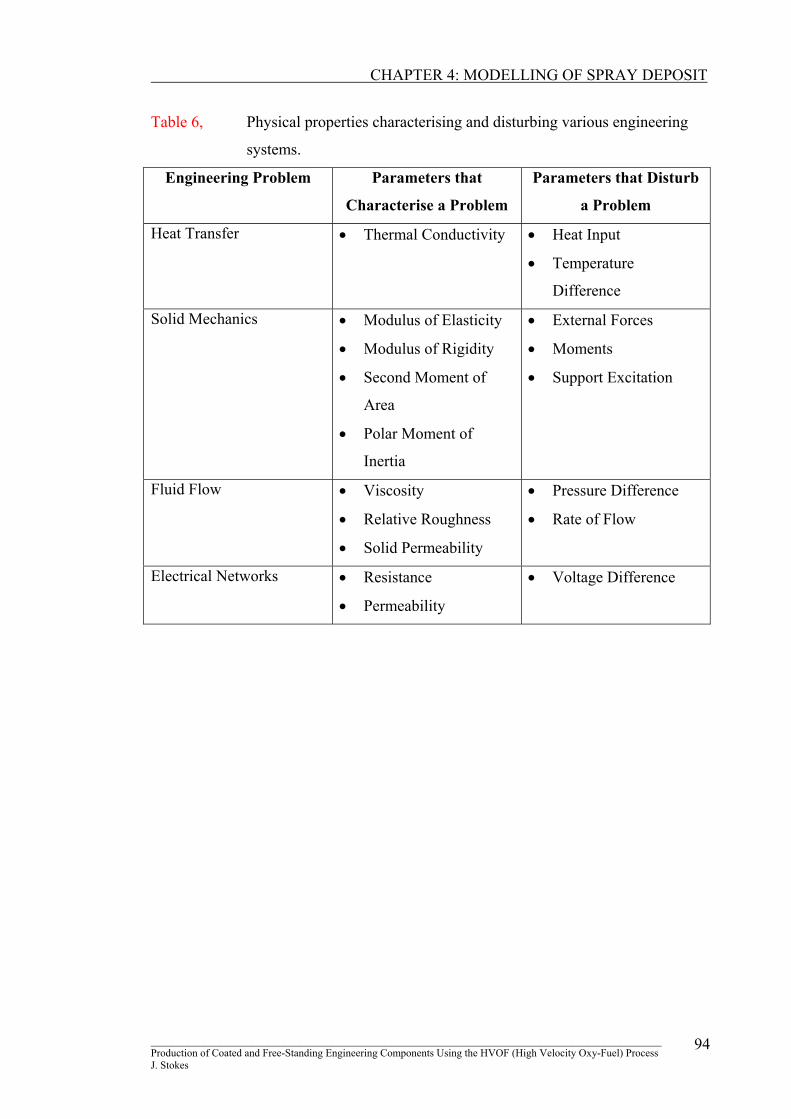
thermal conductivity, modulus of elasticity, and viscosity properties of a material, as

shown in table 6. On the other hand, there are parameters that produce disturbances in

a system and they appear in the particular part of the solution. Examples of disturbing

parameters include temperature difference across a medium, external forces, moments,

and pressure difference in a fluid flow, as shown in table 6.


93


Table 6, Physical properties characterising and disturbing various engineering

systems.

Engineering Problem Parameters that

Characterise a Problem

Parameters that Disturb

a Problem

Heat Transfer • Thermal Conductivity

• Heat Input

• Temperature

Difference

Solid Mechanics • Modulus of Elasticity

• Modulus of Rigidity

• Second Moment of

Area

• Polar Moment of

Inertia

• External Forces

• Moments

• Support Excitation

Fluid Flow • Viscosity

• Relative Roughness

• Solid Permeability

• Pressure Difference

• Rate of Flow

Electrical Networks • Resistance

• Permeability

• Voltage Difference


94


4.3 NUMERICAL METHODS

Many practical engineering problems can only be solved approximately. This inability

to obtain an exact solution may be attributed to either the complex nature of the

governing differential equations or the difficulties that arise from dealing with initial

and boundary conditions [105]. To deal with such problems, numerical approximations

are used. In contrast to analytical solutions, which show the exact behaviour of a

system at any point within the system, numerical solutions approximate exact solutions

only at discrete points. The first step in the numerical procedure is to discretize

(divide) a system into small subsystems known as elements, where their shape is

described by discrete points known as nodes.

There are two types of numerical methods, finite difference methods and finite element

methods. With finite difference methods, the differential equation is written at each

discrete point (node), and the derivatives are replaced by difference equations, this

approach results in a set of simultaneous linear equations [106]. Finite difference

methods are easy to understand in simple systems, however they become difficult to

apply to systems with complex geometries or with complex boundary conditions, an

example of this would be a system involving non-isotropic material properties.

The finite element method use integral formulations, rather than difference equations,

to create a system of algebraic equations. Moreover, an approximate continuous

function is assumed to represent the solution for each element. The complete solution

is generated by connecting or assembling the individual solutions, allowing for

continuity at the inter-elemental boundaries.


95


4.4 STEPS IN THE FINITE ELEMENT METHOD

The basics steps involved in any finite element analysis consist of the following:

Preprocessor Phase

• Create and discretize the solution domain into finite elements, that is the

system is sub-divided into elements and nodes

• Assume a shape function to represent the physical behaviour of an element.

• Develop equations for an element

• Arrange and assemble the elements to present the entire system. Construct

the global stiffness matrix

• Apply boundary conditions, initial conditions and loads

Solution Phase

• Solve a set of linear or non-linear algebraic equations simultaneously to

obtain nodal results, such as displacement values at different nodes or

temperature values at different nodes in a heat transfer system

Postprocessor Phase

• Obtain other important information including stress values, heat fluxes and

so on


96


4.5 NUMERICAL FORMULATION The following examples illustrate the simplified one-dimensional direct formulation

steps used to analyse both heat transfer and residual stress systems experienced in the

current research, with reference to Fagan [105] and Moaveni [106].

4.5.1 Heat Transfer System

A sample consists of a stainless steel substrate, coated with aluminium (releasing

layer), on which a coating of tungsten carbide-cobalt is placed. The following

describes the determination of the temperature distribution through the three materials,

when a heat source is placed near the tungsten carbide-cobalt surface.

Preprocessing Phase

Discretize the solution domain into finite elements.

The system is represented by six nodes (discrete points) and five elements (sub-

systems) as shown in figure 35.

DJ Gun Tflame

5

Element 5

6 Tair (5

Back of Substrate

(11

Element 1

(44

Element 4

Substrate

(33

Element 3

Aluminium

(22

Element 2

WC-Co

Figure 35, Finite Element model for temperature distribution through various

materials.


97


Assume a solution that approximates the behaviour of an element.

In this situation, there are two modes of heat transfer (conduction and convection),

both of which must be understood before formulation of the conductance matrix and

the thermal load matrix. Is must be noted that the solution ignores the fact that heat

loss will be experienced around the sides of the sample, hence an approximation of the

real solution will be found.

The steady state thermal behaviour of the elements (2), (3), and (4) may be modelled

using Fourier’s Law. When there is a temperature gradient in a medium, conduction

heat transfer occurs, as shown in figure 36. The energy is transported from the high-

temperature region to the low-temperature region by molecular activity.

The heat transfer rate is given by Fourier’s Law:

qx = -kA XT

∂∂ Equation 32

qx is the X-component of the heat transfer rate, k is the thermal conductivity of the

medium, A is the area, and XT

∂∂ is the temperature gradient. The minus sign is due to

the fact that heat flows in the direction of decreasing temperature.

Ti+1

Ti

qx

k

X

L

Figure 36, Heat transfer by conduction through a medium.


98


Equation 32 can be written in terms of the spacing between the nodes (length of the

element) L and the respective temperatures of the nodes i and i+1, Ti and Ti+1 by the

following [107]:

q = L

TTkA ii )( 1+− Equation 33

The steady state behaviour of elements (1) and (5) may be modelled using Newton’s

Law of Cooling. Convection heat transfer occurs when a fluid in motion comes into

contact with a surface whose temperature differs from the moving fluid. The overall

heat transfer rate between the fluid and the surface is governed by Newton’s Law of

Cooling [108], by the following equation:

q = hA(Tf – Ts) Equation 34

where h is the heat transfer coefficient (W/m2K), Ts is the surface temperature, and Tf

represents the temperature of the moving fluid (gas). According to Holman [108],

under steady state conduction, the application of energy balance to a surface requires

that the energy transferred to a surface by conduction must be equal to the energy

transferred by convection. Hence,

-kA XT

∂∂ = hA[Tf – Ts] Equation 35

as shown in figure 37.

h (for convection) is given by:

h = Lk Equation 36


99


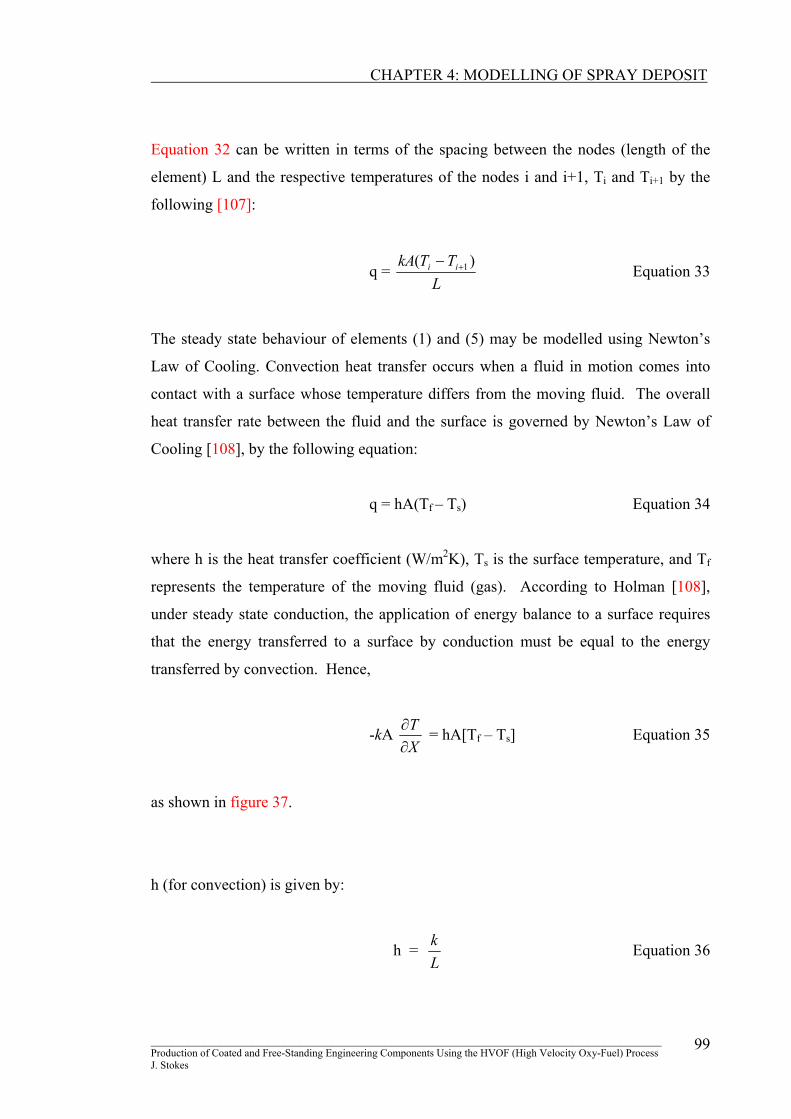
therefore:

kA XT

∂∂ =

LkA (∆T) Equation 37

XT

∂∂qconduction = -kA

qconvection = hA[Tf – Ts]

Tf , h

qconvection qconduction

Ti+1

Ti =Ts k

X

L

Figure 37, Energy balance at a surface with convective heat transfer.

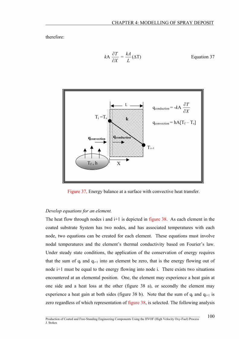
Develop equations for an element.

The heat flow through nodes i and i+1 is depicted in figure 38. As each element in the

coated substrate System has two nodes, and has associated temperatures with each

node, two equations can be created for each element. These equations must involve

nodal temperatures and the element’s thermal conductivity based on Fourier’s law.

Under steady state conditions, the application of the conservation of energy requires

that the sum of qi and qi+1 into an element be zero, that is the energy flowing out of

node i+1 must be equal to the energy flowing into node i. There exists two situations

encountered at an elemental position. One, the element may experience a heat gain at

one side and a heat loss at the other (figure 38 a), or secondly the element may

experience a heat gain at both sides (figure 38 b). Note that the sum of qi and qi+1 is

zero regardless of which representation of figure 38, is selected. The following analysis


100


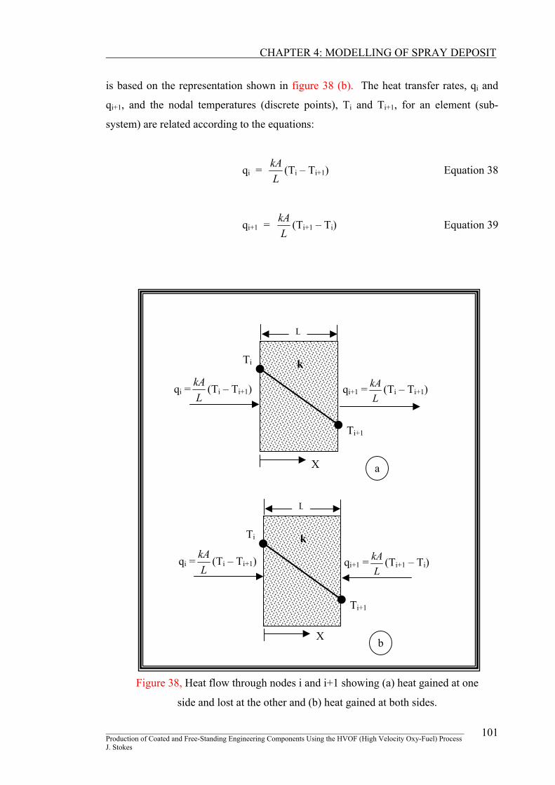
is based on the representation shown in figure 38 (b). The heat transfer rates, qi and

qi+1, and the nodal temperatures (discrete points), Ti and Ti+1, for an element (sub-

system) are related according to the equations:

qi = LkA (Ti – Ti+1) Equation 38

qi+1 = LkA (Ti+1 – Ti) Equation 39

LkA

LkA

LkA

LkA

b

qi = (Ti – Ti+1) qi+1 = (Ti+1 – Ti)

Ti+1

Ti k

X

L

a

qi = (Ti – Ti+1) qi+1 = (Ti – Ti+1)

Ti+1

Ti k

X

L

Figure 38, Heat flow through nodes i and i+1 showing (a) heat gained at one

side and lost at the other and (b) heat gained at both sides.


101


The elemental description given by equations 38 and 39 may be expressed in matrix

form as follows:

+1i

i

qq

= LkA

−

−1111

+1i

i

TT

Equation 40

The thermal conductance matrix for the element shown in figure 38 (b), is given as:

[ ]( ) = eKLkA

−

−1111

Equation 41

Assemble the elements to present the entire system.

Using equation 41 the position matrix for the first element is given by:

[ ]( ) = A1K

−

−

1

1

1

1

1

1

1

1

Lk

Lk

Lk

Lk

Equation 42

and its position in the global conductance matrix (overall matrix to describe the total

system) is given by:

[ ]( )G1K = A

−

−

000000000000000000000000

0000

0000

1

1

1

1

1

1

1

1

Lk

Lk

Lk

Lk

6

5

4

3

2

1

TTTTTT

Equation 43


102


Similar to element 1, the elemental position matrices together with their position in the

global conductance matrix for elements 2, 3, 4 and 5 are given as follows:

[ ]( )2K = A

−

−

2

2

2

2

2

2

2

2

Lk

Lk

Lk

Lk

and [ ]( )G2K = A

−

−

000000000000000000

0000

0000000000

2

2

2

2

2

2

2

2

Lk

Lk

Lk

Lk

6

5

4

3

2

1

TTTTTT

Equation 44

[ ]( )3K = A

−

−

3

3

3

3

3

3

3

3

Lk

Lk

Lk

Lk

and [ ]( )G3K = A

−

−

000000000000

0000

0000000000000000

3

3

3

3

3

3

3

3

Lk

Lk

Lk

Lk

6

5

4

3

2

1

TTTTTT

Equation 45

[ ]( )4K = A

−

−

4

4

4

4

4

4

4

4

Lk

Lk

Lk

Lk

and [ ]( )G4K = A

−

−

000000

0000

0000000000000000000000

4

4

4

4

4

4

4

4

Lk

Lk

Lk

Lk

6

5

4

3

2

1

TTTTTT

Equation 46


103


[ ]( )5K = A

−

−

5

5

5

5

5

5

5

5

Lk

Lk

Lk

Lk

and [ ]( )G5K = A

−

−

5

5

5

5

5

5

5

5

0000

0000000000000000000000000000

Lk

Lk

Lk

Lk

6

5

4

3

2

1

TTTTTT

Equation 47

The overall global conductance matrix (matrix for the system) is given as the sum of

each elemental position:

[K](G) = [K](1G) + [K](2G) + [K](3G) + [K](4G) + [K](5G) Equation 48

Hence the overall global conductance matrix for the coated substrate system shown in

figure 35 is given as follows:

[ ](GK ) = A

−

−+−

−+−

−+−

−+−

−

5

5

5

5

5

5

5

5

4

4

4

4

4

4

4

4

3

3

3

3

3

3

3

3

2

2

2

2

2

2

2

2

1

1

1

1

1

1

1

1

0000

000

000

000

000

0000

Lk

Lk

Lk

Lk

Lk

Lk

Lk

Lk

Lk

Lk

Lk

Lk

Lk

Lk

Lk

Lk

Lk

Lk

Lk

Lk

Equation 49


104


Apply Boundary Conditions and Thermal Loads

Finite element formulation of heat transfer systems, always lead to an equation of the

form [108]:

[K]{T} = {q} Equation 50

[Conductance Matrix]{Temperature Matrix}={Heat Flow Matrix} Equation 51

In this system, the WC-Co coating is exposed to a known flame temperature T1 =

500oC (first boundary condition), and the air temperature behind the substrate T6 =

50oC (second boundary condition). In the case the overall matrix equation is

represented as follows:

A

−

−+−

−+−

−+−

−+−

−

5

5

5

5

5

5

5

5

4

4

4

4

4

4

4

4

3

3

3

3

3

3

3

3

2

2

2

2

2

2

2

2

1

1

1

1

1

1

1

1

0000

000

000

000

000

0000

Lk

Lk

Lk

Lk

Lk

Lk

Lk

Lk

Lk

Lk

Lk

Lk

Lk

Lk

Lk

Lk

Lk

Lk

Lk

Lk

=

Equation 52

6

5

4

3

2

1

TTTTTT

C

C

o

o

500000

500

As matrices are a representation of a series of simultaneous equations, the equation for

the first row and the final row should read as follows:

T1 = 500oC Equation 53

T6 = 50oC Equation 54


105


Therefore rows 1 and 6 are adjusted (by removing the Lk constants) in the global

conductance matrix, to yield the results shown equations 53 and 54 as follows:

A

−+−

−+−

−+−

−+−

A

Lk

Lk

Lk

Lk

Lk

Lk

Lk

Lk

Lk

Lk

Lk

Lk

Lk

Lk

Lk

LkA

100000

000

000

000

000

000001

5

5

5

5

4

4

4

4

4

4

4

4

3

3

3

3

3

3

3

3

2

2

2

2

2

2

2

2

1

1

1

1

6

5

4

3

2

1

TTTTTT

=

Equation 55

C

C

o

o

500000

500

Row two is as follows when multiplied out:

-1

1

LAk T1 +

1

1

LAk T2 +

2

2

LAk T2 -

2

2

LAk T3 = 0 Equation 56

By equation 53:

1

1

LAk T2 +

2

2

LAk T2 -

2

2

LAk T3 = A

1

1

Lk 500 Equation 57

Similarly row five reduces to the following:

-4

4

LAk T4 +

4

4

LAk T5 +

5

5

Lk T5 = A

5

5

Lk 50 Equation 58


106


Ignoring the equations involved in row 1 and 6, and incorporating the known boundary

conditions into rows 2 and 5 of the heat transfer system, equation 55 is reduced to:

A

+−

−+−

−+−

−+

5

5

4

4

4

4

4

4

4

4

3

3

3

3

3

3

3

3

2

2

2

2

2

2

2

2

1

1

00

0

0

00

Lk

Lk

Lk

Lk

Lk

Lk

Lk

Lk

Lk

Lk

Lk

Lk

Lk

Lk

. =

5

4

3

2

TTTT

5000

500

5

5

1

1

Lk

Lk

Equation 59

Substituting the conductivity k values, length L (taken as the heat effected zone

distance for the flame or the thickness of the material) and exposure area (A) values

(latter two taken from the experimental data in the current research, see figure 39), into

equation 59, results in the calculation of the various elemental temperatures (T2-5). The

data shown in table 7 represents a real heat transfer situation:

________________________________________________________________________________________________ Production of Coated and Free-Standing Engineering Components Using the HVOF (High Velocity Oxy-Fuel) Process

107

L3

L4

Stainless Steel

Aluminium

WC-Co

L1

Area A

L2

Figure 39, Schematic of the heat transfer system.

J. Stokes


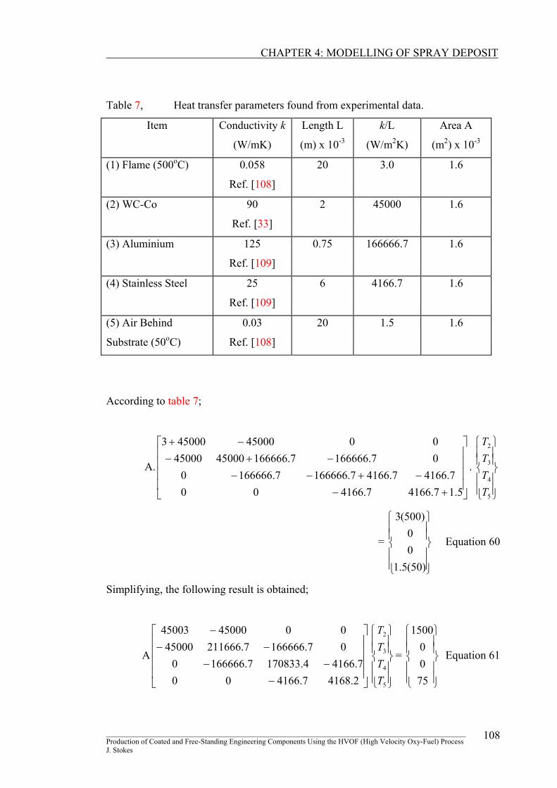
Table 7, Heat transfer parameters found from experimental data.

Item Conductivity k

(W/mK)

Length L

(m) x 10-3

k/L

(W/m2K)

Area A

(m2) x 10-3

(1) Flame (500oC) 0.058

Ref. [108]

20 3.0 1.6

(2) WC-Co 90

Ref. [33]

2 45000 1.6

(3) Aluminium 125

Ref. [109]

0.75 166666.7 1.6

(4) Stainless Steel 25

Ref. [109]

6 4166.7 1.6

(5) Air Behind

Substrate (50oC)

0.03

Ref. [108]

20 1.5 1.6

According to table 7;

A. .

+−−+−−

−+−−+

5.17.41667.4166007.41667.41667.1666667.1666660

07.1666667.16666645000450000045000450003

5

4

3

2

TTTT

= Equation 60

)50(5.100

)500(3

Simplifying, the following result is obtained;

A = Equation 61

−−−

−−−

2.41687.4166007.41664.1708337.1666660

07.1666667.21166645000004500045003

5

4

3

2

TTTT

7500

1500


108


In the present research, convection from the flame at the front and convection with the

air at the back of the sample was ignored. Experimental data provided temperatures

both at the front and back of the sample, hence convection was not required. The

system use is shown in figure 40.

Tback

AluminiumWC-Co Back of Substrate

Tfront (11

Element 1

4

Substrate

(33

Element 3

(22Element

2

Figure 40, Finite Element model used in the present research.

Equation 52 in this case is reduced to:

A

−

−+−

−+−

−

3

3

3

3

3

3

3

3

2

2

2

2

2

2

2

2

1

1

1

1

1

1

1

1

00

0

0

00

Lk

Lk

Lk

Lk

Lk

Lk

Lk

Lk

Lk

Lk

Lk

Lk

. = Equation 62

4

3

2

1

TTTT

000

500

Where 500 is the only known front temperature. Substituting the conductivity k values,

length L (taken as the heat effected zone distance for the flame or the thickness of the

material) and exposure area (A) values (from table 8) into equation 62, results in the

calculation of the various elemental temperatures (T2-4).


109


Table 8, Parameters used in the heat transfer finite element analysis.

Item Conductivity k

(W/mK)

Length L

(m) x 10-3

k/L

(W/m2K)

Area A

(m2) x 10-3

(1) WC-Co 90

Ref. [33]

2 45000 1.6

(2) Aluminium 125

Ref. [109]

0.75 166666.7 1.6

(3) Stainless Steel 25

Ref. [109]

6 4166.7 1.6

A . = Equation 63

−−−

−−−

7.41667.4166007.41664.1708337.1666660

07.1666667.21166645000004500045000

4

3

2

1

TTTT

000

500

Solution Phase

Solve a system of algebraic equations simultaneously.

Solving the previous matrix (equation 63) yields the temperature distribution across the

sample:

4

3

2

1

TTTT

=

98.49998.49999.499

500

oC Equation 64

The results show that the spraying temperature (front temperature) of 500oC, is

reflected in a temperature of 357.8oC, across the substrate (back temperature).

Postprocessing Phase

Obtain other Information.

The solution (equation 64) may be represented as a temperature contour of the thermal

gradient through the sample.


110


4.5.2 Residual Stress Determination

A substrate material (stainless steel) is coated with WC-Co to a certain thickness.

During deposition, stresses (quenching of lamella and cooling of coating) generate,

generating a moment at the ends of the sample, causing the sample to deflect, as shown

in figure 41.

Deflection

Moment

Coating

Substrate

Heat Heat

Figure 41, Moment in a sample generating a deflection.

As explained in an earlier section, the simulation of both the quenching and cooling

stresses in one system is quite difficult, hence the method of simulation used in the

present study relied on the deformation of the final sample post-spraying. To

demonstrate the numerical formulation for this system, two simple approximation

methods were analysed. One method was to apply various temperatures to a coated

sample of known thickness and then measure the stress through the tungsten carbide-

cobalt deposit when the resulting deflection measured in the finite element analysis,

equalled that found experimentally in the Clyne’s Method. In this case the applied

temperature in the finite element system generated a thermal load in the centre of the

beam, and caused the beam to deflect, similar to that used by Steffens et al. [102].

Appendix 7 shows the procedure used to simulate this system.


111


Similarly this system was simulated by applying a known deflection to the sample

(Appendix 7) and compared to the latter. The system was simulated by locking both

ends of the sample while subjecting the centre of the sample to a ‘thermal load’ P (to

generate the deflection), as shown in figure 42. The load and in turn deflection creates

an internal stress in the deposit causing permanent bending in the sample. The elastic

modulus for each material is given as Es (substrate) and Ec (coating). The sample has a

width W, length L, and thicknesses of ts (substrate), and tc (coating). The numerical

formulation for the latter system will be described in the following section.

W

Fixed Point

P

Coating

Substrate

L

tcts

Figure 42, Coated sample subjected to a central displacement.

Preprocessing Phase

Discretize the solution domain into finite elements.

In order to highlight the basic steps in the finite element analysis, the coated sample is

discretize into simple parts. The sample has been divided into four individual segments

called elements, with each segment having a uniform cross-section as shown in figure

43. Each element is represented as an elastic beam with nodes top and bottom of the

element and in turn each element is joined to another element by connecting one node

to the next. The accuracy of the results may be increased, by increasing the number of

additional nodes and elements.


112


5

4

3

2

1

u5

u4

u3

u2

u1

Element 4

Element 3

Element 2

P

Elastic Beam

Element 1

4 2

3 1

P

Figure 43, Sub-dividing the sample into elements and nodes.

Assume a solution that approximates the behaviour of an element.

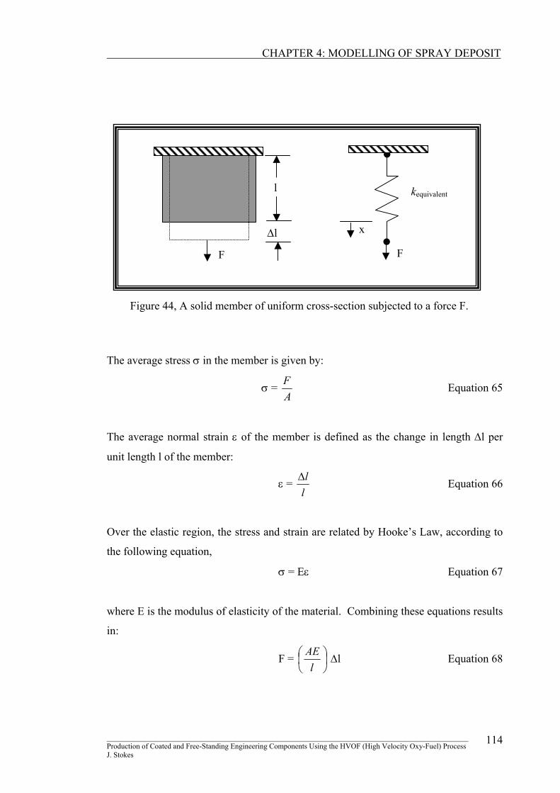
In order to study the behaviour of a typical element, figure 44 shows a solid member

with a uniform cross-section A of a length l subjected to a force F.


113


x

kequivalent

F

∆l

l

F

Figure 44, A solid member of uniform cross-section subjected to a force F.

The average stress σ in the member is given by:

σ = AF Equation 65

The average normal strain ε of the member is defined as the change in length ∆l per

unit length l of the member:

ε = ll∆ Equation 66

Over the elastic region, the stress and strain are related by Hooke’s Law, according to

the following equation,

σ = Eε Equation 67

where E is the modulus of elasticity of the material. Combining these equations results

in:

F =

lAE

∆l Equation 68


114


Equation 68 is similar to the equation for a linear spring, F = kx. Therefore, a centrally

loaded member of uniform cross-section may be modelled as a spring with equivalent

stiffness of

keq = l

AE Equation 69

The coated sample is modelled as a series of centrally loaded members with equal

cross-sections. Thus, the sample is represented by a model consisting of four elastic

springs (elements) in series, and the elastic behaviour of each element is modelled by

an equivalent linear spring according to the equation:

f = keq (ui+1 – ui) = l

AE (ui+1 – ui) Equation 70

ui and ui+1 are the displacements of the member at nodes i and i+1 respectively, and l is

the length of the element.

Develop equations for an element.

As each element has two nodes, and with each node there is an associated

displacement, then the system requires two equations for each element. These

equations must involve nodal displacements and the element’s stiffness. The elemental

relationship between the internally transmitting forces (fi and fi+1), and the end

displacements (ui and ui+1) is shown in figure 45.


115


ui+1ui

Node i

Node i+1

fi+1 = keq (ui+1 – ui)

b

fi = keq (ui – ui+1)

or

y

Node i

Node i+1

fi = keq (ui+1 – ui)

fi+1 = keq (ui+1 – ui)

ui

a

Figure 45, Internally transmitted forces through an arbitrary element.

Static equilibrium conditions require that the sum of fi and fi+1 be equal to zero. In

figure 45, there are two ways (tension or two forces acting in the same directions) to

represent the transmission of forces acting on a member. The representation shown in

figure 45 (b), will be observed, so that the directions of fi and fi+1 are in the same

direction as y. Thus the transmitted forces at nodes i and i+1 are as follows:

fi = keq (ui – ui+1) Equation 71

fi+1 = keq (ui+1 – ui) Equation 72

Equations 72 may be expressed in matrix form as follows:

+1i

i

ff

= Equation 73

−

−

eqeq

eqeq

kkkk

+1i

i

uu


116


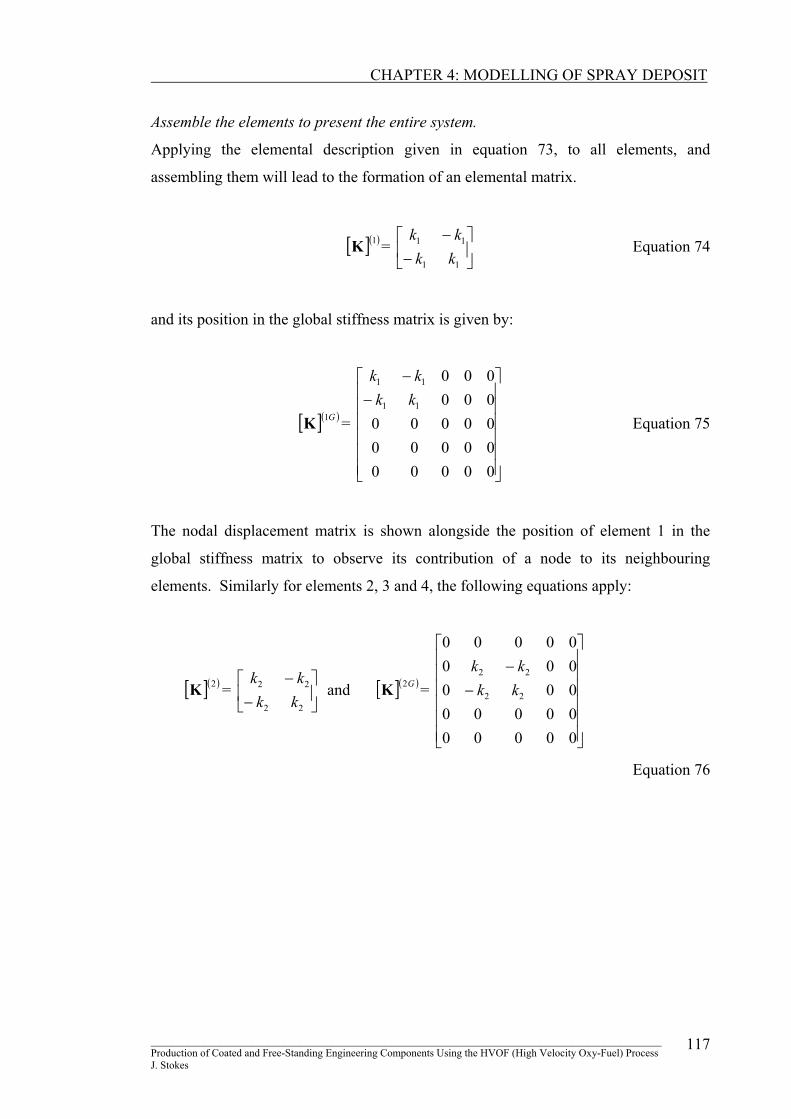
Assemble the elements to present the entire system.

Applying the elemental description given in equation 73, to all elements, and

assembling them will lead to the formation of an elemental matrix.

[ ]( ) = Equation 74 1K

−

−

11

11

kkkk

and its position in the global stiffness matrix is given by:

[ ]( )G1K = Equation 75

−

−

000000000000000000000

11

11

kkkk

The nodal displacement matrix is shown alongside the position of element 1 in the

global stiffness matrix to observe its contribution of a node to its neighbouring

elements. Similarly for elements 2, 3 and 4, the following equations apply:

[ ]( )2K = and

−

−

22

22

kkkk [ ]( )G2K =

Equation 76

−−

000000000000000000000

22

22

kkkk


117


[ ]( )3K = and

−

−

33

33

kkkk [ ]( )G3K =

Equation 77

−−

000000000000000000000

33

33

kkkk

[ ]( )4K = and

−

−

44

44

kkkk [ ]( )G4K =

Equation 78

−−

44

44

000000

000000000000000

kkkk

The final (overall) global stiffness matrix is obtained by assembling, or adding together

each element’s position in the global stiffness matrix:

[K](G) = [K](1G) + [K](2G) + [K](3G) + [K](4G) Equation 79

[ ](GK ) = Equation 80

−−+−

−+−−+−

−

44

4433

3322

2211

11

00000

0000000

kkkkkk

kkkkkkkk

kk

Apply Boundary Conditions and Loads

In this system, the sample is held at both ends while a load P is applied to the centre of

the sample. Applying this condition (adopting equation 73) results in the following set

of linear equations:


118


−−+−

−+−−+−

−

44

4433

3322

2211

11

00000

0000000

kkkkkk

kkkkkkkk

kk

. = Equation 81

5

4

3

2

1

uuuuu

0000P

In solid mechanics systems, the finite element formulation always lead to a general

equation of the form [106]:

[K = Stiffness matrix]{u = Displacement matrix} = {F= Load matrix}

Equation 82

The solution to this system cannot be calculated, as applying a force to a fixed point

will cause no displacement, as explained in figure 46. Where one element (that is

element 1 in figure 45 a) occupies length of the sample (as this is a one-dimensional

system), applying the boundary condition (u1 = 0) to this element prevents the force P

from impacting elements 2, 3, and 4. The numerical matrix formulation depicts a

simple one-dimensional analysis however this problem was performed as a two-

dimensional system (or higher orders) in the current research, hence the elemental

distribution would look more like that shown in figure 45 b. Hence the boundary

condition (u1 = 0) was applied to the lower corners elements of the beam. This

formulation of the system would allow the centre of the sample to deflect. This

highlights the inaccuracy found in results, when using a coarse (fewer elements) mesh.


119


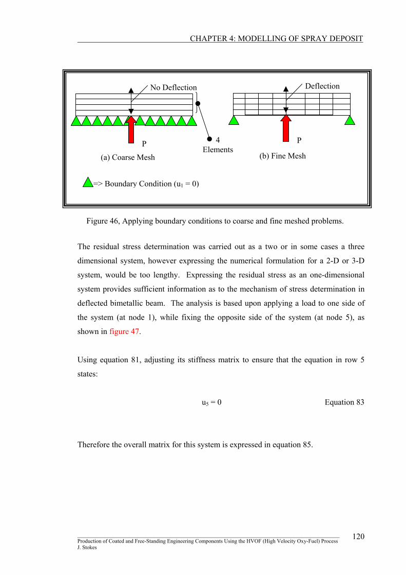
(a) Coarse Mesh (b) Fine Mesh

4 Elements

No Deflection Deflection

=> Boundary Condition (u1 = 0)

P P

Figure 46, Applying boundary conditions to coarse and fine meshed problems.

The residual stress determination was carried out as a two or in some cases a three

dimensional system, however expressing the numerical formulation for a 2-D or 3-D

system, would be too lengthy. Expressing the residual stress as an one-dimensional

system provides sufficient information as to the mechanism of stress determination in

deflected bimetallic beam. The analysis is based upon applying a load to one side of

the system (at node 1), while fixing the opposite side of the system (at node 5), as

shown in figure 47.

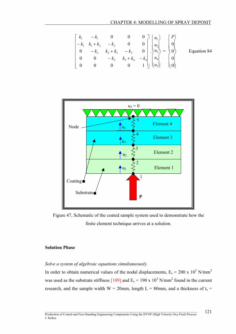
Using equation 81, adjusting its stiffness matrix to ensure that the equation in row 5

states:

u5 = 0 Equation 83

Therefore the overall matrix for this system is expressed in equation 85.


120


−+−−+−

−+−−

1000000

0000000

4433

3322

2211

11

kkkkkkkk

kkkkkk

. = Equation 84

5

4

3

2

1

uuuuu

0000P

Coating

Substrate

Node

Element 1

u5 = 0

5

4

3

2

1

u4

u3

u2

u1

Element 4

Element 3

Element 2

P

Figure 47, Schematic of the coated sample system used to demonstrate how the

finite element technique arrives at a solution.

Solution Phase

Solve a system of algebraic equations simultaneously.

In order to obtain numerical values of the nodal displacements, Es = 200 x 103 N/mm2

was used as the substrate stiffness [109] and Ec = 190 x 103 N/mm2 found in the current

research, and the sample width W = 20mm, length L = 80mm, and a thickness of ts =


121


1mm (substrate), and tc = 1mm (coating), all values used in the experimental section of

the research. The load applied will be assumed to be 5N.

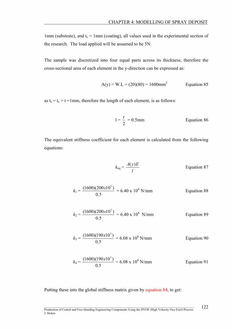
The sample was discretized into four equal parts across its thickness, therefore the

cross-sectional area of each element in the y-direction can be expressed as:

A(y) = W.L = (20)(80) = 1600mm2 Equation 85

as ts = tc = t =1mm, therefore the length of each element, is as follows:

l = 2t = 0.5mm Equation 86

The equivalent stiffness coefficient for each element is calculated from the following

equations:

keq = l

EyA )( Equation 87

k1 = 5.0

)10200)(1600( 3x = 6.40 x 108 N/mm Equation 88

k2 = 5.0

)10200)(1600( 3x = 6.40 x 108 N/mm Equation 89

k3 = 5.0

)10190)(1600( 3x = 6.08 x 108 N/mm Equation 90

k4 = 5.0

)10190)(1600( 3x = 6.08 x 108 N/mm Equation 91

Putting these into the global stiffness matrix given by equation 84, to get:


122


108. . = Equation 92

−−−−

−−−

1000008.616.1208.600

008.648.124.60004.68.124.60004.64.6

5

4

3

2

1

uuuuu

00005

The displacement solution to this matrix is: u1 = 3.2 x 10-8mm, u2 = 2.5 x 10-8mm, u3 =

1.7 x 10-8mm, u4 = 0.8 x 10-8mm, and u5 = 0mm. The force of 5N caused the sample to

deflect by varying displacements from node 1 (highest displacement at point of force)

up to node 5 (no displacement). A contour line representation of this result is shown in

figure 48.

0.5mm

2 mm

u4 Deflection u3 Deflection u2 Deflection u1 Deflection

Figure 48, Schematic of the graphical contour lines showing the displacements of

each node (solid lines) compared to pre-deformed shape (coloured lines).

Postprocessing Phase

Obtain other Information.

Additional information such as average normal stress in each element may be of

concern. These values can be determined from the equation:

σ = avgAf =

avg

iieq

Auuk )( 1 −+ =

avg

iiavg

A

uulEA )( 1 −+ = E

−+

luu ii 1 Equation 93


123


where

−+

luu ii 1 = ε, the strain in each element. The average normal stress through

each element is:

σ(1) = Es

−

luu 12 = (200 x 103)

−5.0

2.35.2 x 10-8 = -280 x10-5 N/mm2

Equation 94

σ(2) = Es

−

luu 23 = (200 x 103)

−5.0

5.27.1 x 10-8 = -320 x10-5 N/mm2

Equation 95

σ(3) = Ec

−

luu 34 = (190 x 103)

−5.0

7.18.0 x 10-8 = -342 x10-5 N/mm2

Equation 96

σ(4) = Ec

−

luu 45 = (190 x 103)

−

5.08.00 x 10-8 = -304 x10-5 N/mm2

Equation 97

The compressive stress is experienced by both the substrate and the coating The

highest stress is found at the interface (bonding) point of the substrate and coating.

The stress is highest here due to the mismatch in stiffness. In the ANSYS program

these stresses would be represented by coloured contours, similar to that shown in

figure 49.


124


N/mm2

-0.0028

-0.00304

-0.0032

-0.00342 Coating

Substrate

Node 4

Node 3

Node 2

Node 1

Figure 49, Schematic of the nodal stress contours based on the numerical formulation

problem used in the present section.

The residual stress was simulation by applying a thermal load to the system (based on

the suggestion from the ANSYS user manual [110]) and in parallel by creating a

moment in the sample (applying a compressive force to the deposit while applying an

equal tensile force to the substrate), as shown in figure 49. Each of these simulations

should yield similar results to that found using Clyne’s Method and stress distributions

through the sample thickness, as all three extend from ‘Beam Bending Theory’. The

objective is to use the finite element analysis as a predictive method for determining

residual stress in deposits.

P -P

P -P

Deposit Substrate

M M

Generated moment generates an upward deflection in the centre of the sample

Figure 50, Generated moment finite element analysis system.


125


4.6 Verification of Results

In recent years, the use of finite element analysis as a design tool has grown rapidly.

User friendly comprehensive packages such as ANSYS have become a common tool in

engineering design [110]. Unfortunately, without proper training or a solid

understanding of the underlying engineering principles on the part of the operator, the

finite element procedures can create errors or incorrect results. Sources of errors

include:

(a) Wrong input data, such as physical properties and dimensions

This mistake may be corrected by listing and verifying the physical properties and

co-ordinates of nodes or keypoints before proceeding any further with the analysis.

Units of the geometrical shape, properties and other influencing parameters must be

consistent.

(b) Selecting inappropriate types of elements

It is important to fully grasp the limitations of a given type of element and

understanding what element types belong to what system type, that is a two

dimensional element would be used in a two dimensional system and so on.

(c) Poor element shape and size after meshing

Inappropriate element shape and size will influence the accuracy of the results. It

is important to understand the difference between free meshing (using mixed-area

element shapes) and mapped meshing (using all quadrilateral area elements or

hexahedral volume elements) and the limitations associated with them.

(d) Applying wrong boundary conditions and loads

This step is usually the most difficult aspect of modelling [110]. It involves taking

an actual system and estimating the loading and the appropriate boundary

conditions for the finite element model.

Experimental testing (as carried out in this research) is the best way to check, verify

and predict finite element results. Where finite element results are not verified by


126


experimental results (due to the expense and time consumption in producing

experimental results), verification of finite element results may be found by other

methods, such as comparing results to simply analytical solutions. Applying

equilibrium conditions and energy balance to different parts of the model, to ensure

that the physical laws are not violated is one method of verification. In static models,

the sum of forces acting on a body must equal zero. In heat transfer systems under

steady state conditions, the conservation of energies flowing in and out of nodes should

be balanced.


127


4.7 CAPABILITIES AND ORGANISATION OF ANSYS

The basic steps involved in creating and analysing a model with ANSYS are described

in this section. There are three processors used in ANSYS: (1) the Preprocessor

(PREP7), (2) the Processor (SOLUTION), and (3) the general Postprocessor

(POST1).

4.7.1 Creating A Model With ANSYS: Preprocessor

The preprocessor (PREP7) contains the commands needed to build a model, such as

creating a model geometry and defining element types and element real constants and

material properties, and defining meshing controls and to mesh the object created.

Creating a Model Geometry

There are two methods provided by ANSYS to construct a finite element model’s

geometry, direct or manual generation and the solid-modelling approach. Direct

generation is a simple method where the user specifies the location of nodes and

manually defines which nodes makes up an element. This approach is generally

applied to simple systems that can be modelled with line elements, such as links or

beams, similar to that shown in figure 51 (a). While in the solid-modelling approach,

simple primitives (geometrical shapes such as rectangles, circles, polygons, blocks,

cylinders, and spheres) are used to construct the model, as shown in figure 51 (b).

Boolean operations (such as addition, subtraction, and intersection) are then used to

combine the primitives.


128


(b)

Elemental ModelBoolean Operations Problem

Finite Element Model Problem

Subtract

Add

(a)

Loaded Bridge Node Line Element

Figure 51, Finite element model generation, (a) direct generation, (b) solid modelling

approach.

When creating primitives such as rectangles, the object is made up of entities including

keypoints, lines, and areas or volumes. Keypoints define the vertices of an object, lines

are used to represent the edges of the object, areas or volumes are used to represent

either two or three-dimensional solid objects respectively, as shown in figure 52.

These entities are automatically numbered by the ANSYS program, for data logging.

In general volumes are bounded by areas, areas are bounded by lines, and lines are

bounded by keypoints.


129


Figure 52, The relationship between keypoints, lines and areas.

K = Keypoint L = Line A = Area L4 L2

L1

L3

A1

K2

K2

K4

K1

Element Type Options

ANSYS provides more than one hundred various element types, all of which may be

used to analyse systems. Selecting the correct type of element type to use in a

particular system, is crucial in deriving a ‘true’ solution. Elements may be of three

types: one, two and three-dimensional elements.

The structural and heat transfer systems analysed earlier in the report, were both

analysed using one-dimensional elements. The element is represented by a line

bounded by two nodes, and acts in one direction. The line acts like a spring extending

or compressing depending on the change of its state, as shown in figure 53.

Where an object reacts in two directions due to some external condition, two-

dimensional elements are required to model the system. One-dimensional solutions are

approximated by line segments, whereas the two-dimensional solutions are represented

by plane segments. These two-dimensional plane functions may be in the form of

rectangular elements (4 nodes), quadratic quadrilateral elements (8 nodes), triangular

elements (3 nodes), or quadratic triangular elements (6 nodes), as shown in figure 54

[111].


130


Problem Compressed

Beam 3

(1-Dimensional) Element Model

Spring

Representation

Solution in Both Cases

Figure 53, One-dimensional representation of a problem.

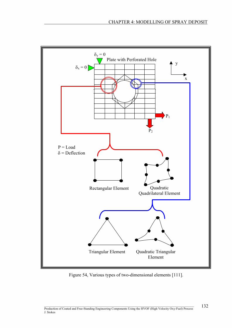
An example of a thin plate with a perforated hole, held at the top left hand corner

(boundary condition, δx&y) and subjected to an applied load P1&2, is shown in figure 54.

This depicts the four possible types of two-dimensional elements that may be found.

Numerical equations apply in a similar way to two-dimensional elements as to one-

dimensional elements, however in figure 54, nodal displacements are calculated in both

x and y directions. A simple way to describe how an element behaves due to an

external condition, is to imagine that each line that bounds a two dimensional element,

reacts like springs, as shown in figure 55.

Just as a two-dimensional object reacts to external stimuli in two directions, a three-

dimensional object with react in three directions. Examples of three-dimensional

elements are brick elements (8 and 20 nodes) and tetrahedral (4 and 10 nodes) as

shown in figure 56 [111].


131


Rectangular Element Quadratic Quadrilateral Element

Triangular Element Quadratic Triangular Element

Plate with Perforated Hole

P1

P2

δy = 0

δx = 0

P = Load δ = Deflection

y

x

Figure 54, Various types of two-dimensional elements [111].


132


kx

kx

ky ky

P

(a) (b) (c)

Figure 55, Simple representation of a two-dimensional element (a), as a series of

springs (b) and subjected to a load (c).

z

y x

10 Node 4 Node

20 Node 8 Node

Figure 56, Schematic of various three-dimensional elements.


133


ANSYS Element Types Used In Research

As described, there are many element types to choose from, and the selection of the

correct element for a specific system is important. The ANSYS user manual [110],

lists the correct element types to use for specific systems, hence this is how the

following element types were chosen. The detail of each element, is a synopsis of the

detail given in the ANSYS manual [111].

Heat Transfer:

PLANE55 is a four-node quadrilateral element used in two-dimensional heat

conduction systems. The element is defined by four nodes, with one degree of freedom

at each node, temperature. Output data include nodal temperatures and elemental data,

such as thermal gradient and thermal flux components.

PLANE77 is an eight-node quadrilateral element used in the modelling of two-

dimensional heat conduction systems. It is basically a higher order version of the

PLANE55 element. The element is capable of modelling systems with curved

boundaries. At each node, the element has a single degree of freedom, temperature.

Output data of this element type include nodal temperatures and elemental data, such

as thermal gradient and thermal flux components.

SOLID70 is a three-dimensional brick element used to model conduction heat transfer

systems. It has eight nodes having a single degree of freedom, temperature.

Convection or heat fluxes are applied to the element’s surface. In addition heat

generation rates may be applied at the nodes. The element may be used to analyse

steady-state or transient systems. The solution output consists of nodal temperatures

and average face temperature, temperature-gradient components and the heat-flux

components.


134


Residual Stress:

PLANE13 has a 2-D magnetic, thermal, electrical, piezoelectric, and structural field

capability with limited coupling between the fields (thermal properties can be inputted

into the system, while stresses may be outputted). PLANE13 is defined by four nodes

with up to four degrees of freedom per node. The element has non-linear magnetic

capability for modelling B-H curves or permanent magnet demagnetization curves.

When used in a structural analysis PLANE13 has large deflection, large strain, and

stress stiffening capabilities.

PLANE42 is a four-node quadrilateral element used in two-dimensional solid

modelling systems. The element is defined by four nodes, with two degrees of freedom

at each node, the translation in the x and y-directions. The element input data can

include thickness if KEYOPTION 3 (plane stress with thickness input) is selected.

Surface pressure loads may be applied to the element edges. Output data include nodal

displacements and elemental data, such as directional stresses and principal stresses.

PLANE82 is an eight-node quadrilateral element used in two-dimensional solid

modelling systems. It is a higher order version of the two-dimensional PLANE42

element. This element offers more accuracy when modelling systems with curved

boundaries. At each node, there are two degree of freedom, the translation in the x and

y-directions. Just like PLANE42, the element input data can include thickness if

KEYOPTION 3 (plane stress with thickness input) is selected. Surface pressure loads

may be applied to the element edges. Output data include nodal displacements and

elemental data, such as directional stresses and principal stresses.

SOLID45 is an eight-node brick element used to model isotropic solid systems. Each

node has three translational degrees of freedom in the nodal x, y and z-directions.

Distributed surface loads may be applied to the element surfaces. This element is used

to analyse large deflections, large strain, plasticity and creep systems. The output

solution data consists of nodal displacements and elemental data, such as stresses in the

x, y, and z directions, shear stresses and principal stresses.


135


SOLID186 is a higher order 3-D 20-node structural solid element with a block

displacement behaviour (deforms in all three x, y and z-directions) and is well suited to

modelling complex shapes (such as those produced by various CAD/CAM systems).

The element has three degrees of freedom per node: translations in the nodal x, y, and z

directions. The element supports plasticity, hyperelasticity, creep, stress stiffening,

large deflection, and large strain capabilities

Finally, it may be worth noting that in general, better results and greater accuracy are

achieved with higher order elements, however these elements require more

computational time [111]. This time requirement is due to the numerical integration of

more complex elemental matrices involved in the calculation of the solution.

Element Real Constants

Element real constants are quantities that are specific to a particular element. For

example, a beam element requires a cross-sectional area, second moment of area and

so on, therefore these real constants vary from one element type to another,

furthermore not all elements require real constants. If the analyst has not used the real

constant, an ANSYS warning prompts as to the missing information.

Material Properties

Physical properties of the model must be defined, before the solution can be calculated.

For example, the modulus of elasticity, Poisson’s ratio or the density of the material

must be defined in solid structural systems, whereas in thermal systems, thermal

conductivity, specific heat, or the density of the material must be defined.

Define Meshing Controls

The finite element model geometry is divided into nodes and elements, a process

known as meshing. The ANSYS program automatically generates the nodes and

specified elements, once the element attributes and element size have been specified:

a) The element attributes include element type or types, real constants, and material

properties.


136


b) The element size controls the coarseness or fineness of the mesh. The larger the

element size, the coarser the mesh, conversely the smaller the element size, the

finer the mesh. If an element edge length of 10 units (unit will depend on the

dimensional unit used to create the model, like millimetres) is specified, then the

ANSYS program will generate a mesh of a series of elements with edge lengths no

larger than 10 units. Another way to control the mesh size is by specifying the

number of element divisions along a boundary line.

Meshing the Model Once the meshing controls have been entered, meshing of the model may commence.

Clicking on the ‘Meshing’ icon, meshing may be applied to areas or the entire volume.

The meshing process can take some time, depending on the model complexity and the

speed of the user’s computer. During the meshing, ANSYS writes a meshing status to

an output window.

There are two types of meshing options that can be used: free and mapped meshing.

Free meshing uses either mixed area element shapes (triangular elements mixed with

quadrilateral elements) or all triangular area elements. The mapped meshing options,

uses all quadrilateral area elements and all hexahedral (brick) volume elements.

Mapped area mesh requires the object to be analysed to have three or four sides, an

equal number of elements on opposite sides of a four sided object, and an even

numbers of elements on all sides of a three sided object. If an object is bound by more

than four lines, the concatenate command is used to combine some of the area edge

lines to form elements, to reduce the total number of lines.

4.7.2 Solution

The solution processor (SOLUTION) has the commands that allow you to apply

boundary conditions and loads. Once all of the boundary information is made

available to the solution processor (SOLUTION), it solves for the nodal solutions.


137


4.7.3 General Postprocessor

The general postprocessor (POST1) contains the commands to read the results data

from the results file, read element results data, plot results and list results of an

analysis. There are other processors that perform additional tasks, such as the Time-

History Processor (POST26), which contains the commands to review results over

time in a transient analysis at a certain point in the model [112]. The Design

Optimisation Processor (OPT) allows the user perform a design optimisation analysis.


138



139

4.8 ANSYS PROCEDURE The procedure used in the current research, for both the heat transfer system and the

residual stress determination is contained in Appendix 7. The procedure describes the

following:

• Describing the system

• Building the geometry in the Preprocessor Phase

• Defining material properties

• Selecting the element type

• Generating the mesh

• Applying the boundary conditions in the Solution Phase

• Solving the system

• Obtaining the solution in the Postprocessor Phase

• Saving and exiting the ANSYS program

Documents

MODELLING OF SPRAY DEPOSIT - DCU HomeCHAPTER 4: MODELLING OF SPRAY DEPOSIT 4 MODELLING OF SPRAY DEPOSIT 4.1 FINITE ELEMENT ANALYSIS The finite element method is a numerical procedure,