Aalborg University Denmark

9th semester at the K-sector Jesper Poulsen

Carsten Lund Lauridsen

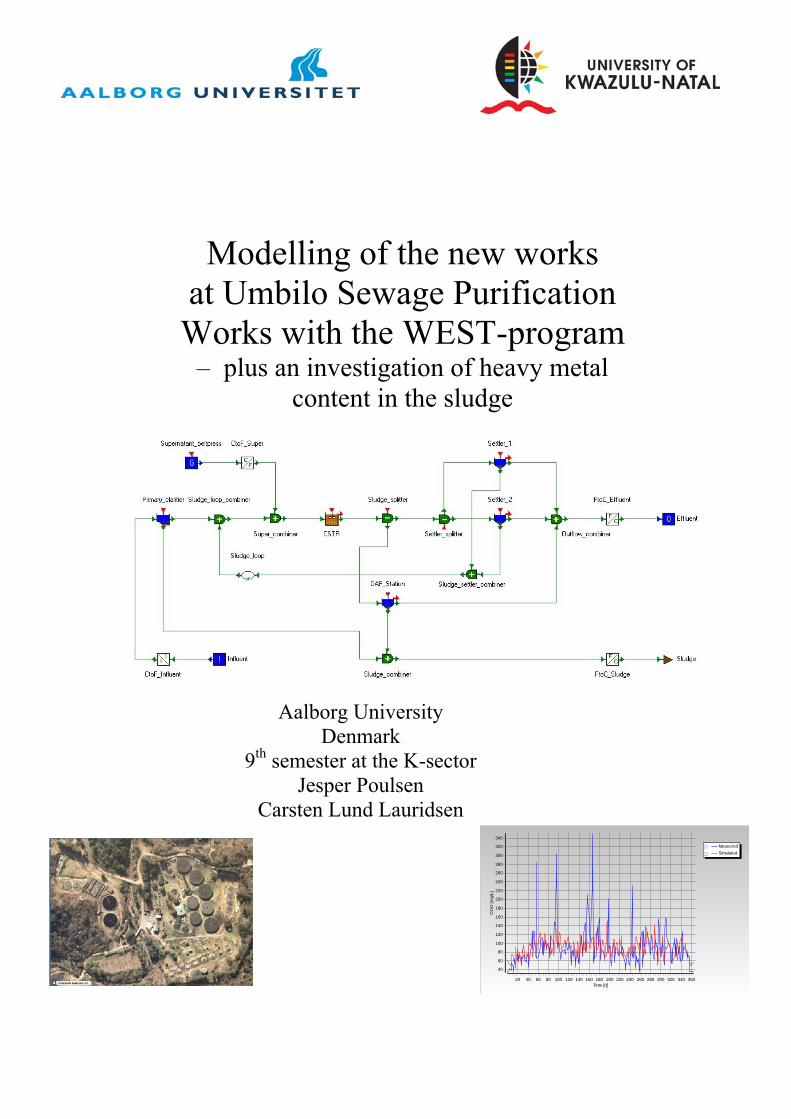
Modelling of the new works at Umbilo Sewage Purification

Works with the WEST-program – plus an investigation of heavy metal

content in the sludge

MeasuredSimulated

Time [d]36034032030028026024022020018016014012010080604020

CO

D [m

g/L]

340

320

300

280

260

240

220

200

180

160

140

120

100

80

60

40

Department of Life Science Study board for chemical and environmental engineering plus biotechnology Sohngaardsholmsvej 57 9000 Aalborg, Denmark Telephone: +45 96 359935 / Fax: + 45 98 140980

Title Modelling of the new works at Umbilo Sewage Purification Works with the WEST-program – plus an investigation of heavy metal content in the sludge

SYNOPSIS The report presents a model to describe the treatment processes in the new works at Umbilo Sewage Purification Works. The commercial WEST program is used for this purpose. A sub-model is used to describe the biological treatment processes in the activated sludge unit, which is operated as a continuously stirred reactor. The sub-model is based on the activated sludge model No. 2 but modified to suit the actual conditions in the reactor. In order to make the sub-model unique for the conditions at the new works, oxygen uptake rates and nitrogen uptake rates experiments are performed. The experiments are used to determine 3 COD fractions in the influent to the plant and 9 model specific parameters. The calibrated and validated model can predict trends and average loads in the effluent for COD, ammonium and nitrate. The model cannot precisely simulate fluctuations. One optimization scenario revealed that the COD and ammonium concentration are reduced respectively 11 mg O2/L and 4 mg N/L when the average oxygen concentration in the activated sludge unit is raised from 0,2 to 2,3 mg O2/L. It is recommended that the overall aeration time for the four surface aerators are increased to a level corresponding to app. 2 mg O2/L. Installation of oxygen probes is needed to control this. The heavy metals content in the sludge from the wastewater treatment plant restricts the sludge being used for agricultural purposes. In order for this to happen the concentration from the industry must not exceed the following concentrations; cadmium 360 mg/m3, copper 1.030 mg/m3 and lead 1.550 mg/m3, where 500 kg sludge is distributed per hectare per year.

Participants in the group Jesper Poulsen Carsten Lund Lauridsen Tutors Associate professor Tjalfe G. Poulsen Professor Jens Aage Hansen Professor Chris A. Buckley Semester 9th semester – Environmental engineering Project period August 2004 – March 2005 Number of copies 8 Number of pages 74

i

ii

Preface This report is prepared at the 9th semester of the master degree in environmental engineering at Aalborg University, Denmark, in connection with a 4-month study period abroad at the University of Kwazulu-Natal, Durban, South Africa. The objective of the report is to model the new works at Umbilo Sewage Purifications Works in the WEST program as a part of the vision for Durban Metropolitan. The long-term vision for Durban Metropolitan is to model all wastewater treatment plants in the Durban Metropolitan Area and using the models as an integral part of the goal to reduce the eutrophication of the rivers in the area. The report is addressed to Durban Metropolitan, the engineer and co-workers at Umbilo Sewage Purification Works plus people with an interest for modelling of wastewater treatment plants. The report is divided into chapters, where the figures, tables and equations are consecutive numbered within each chapter. Appendixes and annexes are placed at the back of the report, where appendixes are numbered with letters and the annexes with roman numerals. The report includes a CD-ROM, where a number of electronically annexes are available. The cite references are indicated after the Harvard-method, which uses the authors surname and publishing year, e.g. [Okking, 2004]. Websites are listed according to the main site. Personal comments are listed with the abbreviation Pers.Com. and the person’s surname. The list of references is placed in the back of the main report. We would like to direct thanks to the following persons in connection with the project and our stay in South Africa:

- Professor Chris Buckley, Head of the Pollution Research Group, University of Kwazulu-Natal, for giving us the opportunity to come to South Africa and the theme to the project. We would also like to thank him for inviting us to a beer at the local pubs.

- Dildar, process engineer at Umbilo Sewage Purification Works, for having the time to answer questions about the plant.

- Lameck Mjadu, superintendent at Umbilo Sewage Purification Works, for allowing us to come to the plant both night and day.

- The workers at Umbilo Sewage Purification Works for helping with the collection of both composite and grab samples.

- Brian Hutcheson, laboratory technician at Umbilo Sewage Purification Works, for performing tests on sewage samples.

- Chris Fennemore and Linda Ndlela, eThekwini Municipality, water and sanitation, for answering question about the Durban Metropolitan area.

- Kerri Hudson, Tamren Ridgway, Rob Stone and the rest of the students at PRG for helping us in the laboratory and making us fell welcome in South Africa.

Aalborg University, March 2005

_____________________________ _____________________________ Jesper Poulsen Carsten Lund Lauridsen

iii

Table of contents Preface......................................................................................... iii Table of contents ........................................................................ iv 1 Introduction........................................................................... 1

1.1 Background for wastewater treatment in South Africa ............ 1 1.2 Durban Metropolitan as sample area .......................................... 2 1.3 WEST as modelling program ....................................................... 3 1.4 Umbilo Sewage Purification Works as study site ....................... 3

2 Project objectives and structure .......................................... 5 2.1 Project objectives ........................................................................... 5 2.2 Project structure ............................................................................ 6

3 Site description ...................................................................... 9 3.1 Catchment area of Umbilo Sewage Purification Works............ 9

3.1.1 Companies in the catchment area ....................................................... 10 3.2 Umbilo river ................................................................................. 11 3.3 Layout of Umbilo Sewage Purification Works ......................... 11

3.3.1 Layout of the old works ........................................................................ 13 3.3.2 Layout of the new works ...................................................................... 15 3.3.3 Layout of the anaerobic digesters........................................................ 17

3.4 Flow balance over Umbilo Sewage Purification Works .......... 18 4 Characterisation of influent and effluent.......................... 20

4.1 Influent characterisation............................................................. 20 4.1.1 Dynamics in the flow............................................................................. 20 4.1.2 Constituents in the wastewater ............................................................ 22

4.2 Discharge demands for effluent ................................................. 23 5 Theory for CSTR model and experiments........................ 25

5.1 Activated sludge model ............................................................... 25 5.1.1 CSTR model........................................................................................... 26

5.2 Methods and procedures to determine model input ................ 30 5.2.1 Performed experiments ........................................................................ 30 5.2.2 Procedure for experiment No. 1........................................................... 31 5.2.3 Procedure for experiment No. 2........................................................... 32 5.2.4 Procedure for experiment No. 3........................................................... 32

6 Determination of COD fractions and parameters............ 33 6.1 Graphical presentation of results............................................... 33

6.1.1 Experiment No. 1................................................................................... 33 6.1.2 Experiment No. 2................................................................................... 33 6.1.3 Experiment No. 3................................................................................... 36

6.2 Summary of results...................................................................... 38

iv

7 WEST-Model .......................................................................40 7.1 Introduction to the WEST program.......................................... 40

7.1.1 Subprograms..........................................................................................40 7.1.2 WEST solution procedure ....................................................................41

7.2 Implementation of the new works in the WEST program...... 42 7.2.1 Selection of sub-models .........................................................................43

7.3 Calibration of the model in the WEST program ..................... 45 7.3.1 Assessment of model results without calibration................................46 7.3.2 Preliminary investigation of the available data set ............................46 7.3.3 Calibration .............................................................................................47

7.4 Validation ..................................................................................... 54 8 Optimization of the CSTR at UPSW..................................56

8.1 The oxygen concentration in the CSTR is raised ..................... 56 8.2 The sludge concentration in the CSTR is increased ................ 56 8.3 The sludge age in the CSTR is increased .................................. 57 8.4 The present design is changed to a “traditionally” design...... 57 8.5 Results from the four scenarios ................................................. 58 8.6 The effect on legislation with the optimized configuration ..... 59

9 Maximum allowed discharge of heavy metals...................60 9.1 Requirements for sludge used for agricultural purposes ........ 60

9.1.1 Discharge standards of sludge and effluent for heavy metals ...........60 9.1.2 Evaluation of the present heavy metal concentrations ......................61 9.1.3 Quantities of heavy metals in domestic sewage ..................................62 9.1.4 Quantities of heavy metals in influent, effluent and sludge...............63 9.1.5 Calculation of maximum allowed quantities from the industry .......64 9.1.6 Disposal and utilization of sludge.........................................................66

10 Conclusion .........................................................................67 11 Perspectivation..................................................................68 12 References..........................................................................70

v

vi

1 Introduction 1.1 Background for wastewater treatment in South Africa It is estimated that South Africa’s total annual water credit is 34 billion m3, but with an annual consumption of 19 billion m3 water in 1990 and rapidly rising, it is estimated that by the year 2020 the water supply is not able to meet the demand. This means, that water will become an ever increasingly scarce strategic resource. The South African water legislation states that water used for industrial and municipal purposes must be returned to its stream of origin, if it is practical possible and purified to meet certain standards [PRG, 1982]. This is done to meet the ever-increasing water demand, but even though it makes up a considerable supplementary source of water, it also deteriorates the water quality. As the public trustee of the nation’s water resources the National Government established in 1998 the third water act in South African history to ensure that water is protected, used, developed, conserved, managed and controlled in a sustainable and equitable manner. The water act addresses some of the disadvantages of the previously water act from 1956 such as non-point pollution sources and makes the new law more streamlined and easier to administrate. The new water act has three discharge standards, which the effluent discharged to a body of water has to comply with. The purpose of the standards is to protect the aquatic ecosystems and to reduce pollution and degradation of the water resources. The standard for some components in the water act of 1998 is tightened compared to the water act of 1956 especially the discharge demands on heavy metals. In appendix A is a description, on how the South African water legislation came into existence. [Uys, 1996] South Africa’s industry is under pressure from two different sides. Since the apartheid was overthrown in 1994, the government has struggled to get jobs for every one; whites as well as coloured and blacks. This means that the industry has to create new jobs. On the other hand as people become more aware of the environment, there is more pressure on the government to provide a good and clean environment. The industry is therefore forced to conserve water more efficiently and reduce contaminants in the effluent. Two of the most important industries for the labour market and economy in the country are textile and metal finishing industry. Unfortunately both sectors use large quantities of water and the resultant contaminated wastewaters negatively affect receiving water bodies. The textile and metal finishing industry use batch reactors in the manufacturing process. This means the load to the wastewater treatment plants is not evenly distributed, but comes in shock-loads when the companies empty the batch reactors. This can be prevented, if all the companies invest in holding tanks, where the industrial effluent is slowly discharged to the sewer pipes. [Barclay, 1996] The South African textile industry is the sixth largest employer in the manufacturing sector in the country with 80.000 people employed directly in the sector and in addition it supports 80.000 cotton workers. There are an additional 200.000 indirectly employed in dependent industries. [Barclay, 1996] A typical textile company uses 150 to 400 litres of water to produce 1 kg of product, hence large quantities of textile effluent have to be disposed. Textile effluent usually has a high COD-count, and a shift over the last decades in the types of dyes used means that most of the dyes are hardly biodegradable, hence giving colour and COD problems for the wastewater treatment plants. [PRG, 1990]

1

Since a lot of companies in the metal finishing industry operate from small backyard shops or as part of a larger manufacturing process, it is difficult to estimate an accurate size of this industry. The annual water consumption by the metal finishing industry was in the region of 9 million m3 in 1987 or between 0,03 to 1,25 m3 water per m2 product and at that time it was app. 0,7% of the total water use by the industrial sector in South Africa. Approximately 80% of the intake water used in the metal finishing industry is discharged as effluent. The effluent from metal finishing companies can have a high content of cyanide complexes, hexavalent chromium as well as several heavy metals. The toxicity of the substances makes it very difficult to treat at the wastewater treatment plants and usually there is some kind of preliminary treatment at the companies, before it is discharged to the sewer pipes. [Binnie and Partners, 1987] A sample area is chosen, where there is high water consumption and the industry in the area consists of both metal finishing and textile companies. Durban Metropolitan Area (DMA) is characterized as the fastest growing metropole and so are the water consumption and the volumes of sewage requiring treatment and disposal. In addition a higher proportion of residents are using water-borne sanitation as informal settlements are being upgraded. [www.local.gov.za, 2005] More than 40% of the country’s textile companies are located in Durban city or the suburban areas of Durban, where also metal finishing factories operate [www.fdimagazine.com, 2005]. DMA is chosen as the sample area because it is assessed that DMA is representative for areas with high water consumption and the mentioned industry.

1.2 Durban Metropolitan as sample area DMA is the second largest metropolitan of the six in the country and covers an area of 2.300 km2 with a population around 3 million. DMA has 14 rivers and most of these are used for recreation purposes. DMA keep records for 6 of the rivers, which have a mean annul run-off of 1.000 million m3. In a few poorly serviced areas, some residents still rely directly on streams for their daily water supply. [www.durban.gov.za, 2005] DMA has 32 wastewater treatment plants, where 21 of these with a total design capacity of 320 million m3 per year discharge their final treated effluent into the main channel of the nearest river. These waters are exposed to contamination, especially nutrient enrichment even if legislation is met, because the general standard only include a discharge standard for ammonium and no other standard for nitrogen and phosphorous. Water quality data indicates that the rivers are eutrofied to a greater or lesser extent depending on the time of the year, where evidence of an enriched condition will be more pronounced, where the base flow of the river is dominated by the continuous flow from the wastewater works, such condition pertains especially during the winter. In half of the rivers the final treated effluent make up app. 90% of the base flow during winter and about 50% of the flow during summer. The data also states that the distance between the wastewater works effluent and the estuary is insufficient to allow the rivers to immobilise the pollutants, hence the estuarine areas become the primary repository for land derived pollutants. The two largest wastewater treatment works with a total design capacity of 170 million m3 per year dispose of effluent to the sea through submarine pipelines. This results in loss of freshwater but also a gain in nutrients for the marine environment with risk for algae blooms as the outcome. [www.durban.gov.za, 2005] The majority of sludge waste produced by treatment plants in the DMA is disposed on landfills, where commercial and industrial activities are the main sources to hazardous waste. There is currently adequate capacity to dispose of domestic and low hazardous waste in DMA, but future capacity is limited. DMA does not have facilities for the disposal of

2

highly hazardous waste defined as any matter that has toxic, chemical or long-lasting properties, which could be harmful to human health and/or the environment. It is therefore of great importance that the industries and the treatment plants in the area have an effective reduction of toxic components in the sludge so non-hazardous landfills can be used for dumping or even better the waste can be used for agriculture purposes. [www.durban.gov.za, 2005] In the light of the above Durban Metropolitan has drawn up an Environmental Management Policy, where two of the main goals are:

• Improve the water quality by making the wastewater treatment plants more effective.

• Reduce and manage hazardous materials produced and disposed in DMA. One of the ways for Durban Metropolitan to fulfil its goals is to model the wastewater treatment plants in the area and thereby have a tool for optimizing and controlling the treatment processes. The long term vision from Durban Metropolitan is to connect the models of wastewater treatment plants with a model for the receiving river. The plan for every river, which receives treated effluent, is to form a large-scale model with interacting models of wastewater treatment plants and the river. Durban Metropolitan then has several large-scale models that can be a useful tool to predict and control the eutrofied environment in the rivers. Durban Metropolitan has joined with the University of KwaZulu-Natal in Durban to solve this task. The university wants to use the WEST program to model the wastewater treatment plants and eventually the rivers.

1.3 WEST as modelling program WEST (Worldwide Engine for Simulation, Training and automation) was developed in the early 1990´s at the University of Ghent in Belgium. WEST is considered to be a powerful tool for dynamic modelling, simulation and optimization and can be used to model wastewater treatment plants, rivers and catchment areas etc. [www.hemmis.com, 2004] Umbilo Sewage Purification Works is one of the wastewater treatment plants in DMA, which has not been modelled prior to this report. It is therefore assigned as the wastewater treatment plant to be modelled in WEST. Umbilo Sewage Purification Works is also interesting, because its influents consist of 20% industrial sewage with the main part deriving from textile and metal finishing factories. The composition of the raw sewage can thereby be assessed as representative for areas with the industry of interest in DMA.

1.4 Umbilo Sewage Purification Works as study site Umbilo Sewage Purification Works (USPW) is situated at the bottom of Paradise Valley in Pinetown in DMA. The plant is divided into two works, the old works and the new works, where both works consists of mechanical and biological treatment together with the addition of chlorine. The biological treatment at the old works consists of trickling filters, whereas the new works have an activated sludge unit operated as a continuously stirred reactor as biological treatment. The plant is described in further details in section 3.3. USPW discharges treated effluent to Umbilo river along with sludge being dumped on landfills situated in DMA. The allowed effluent and sludge concentrations from the plant are governed by South African water legislation. Due to the industrial content in the raw sewage

3

USPW has problems with high contents of organic matter in the effluent and heavy metals in the sludge as described below.

• USPW is designed for an organic load of 500 mg COD/L, but fluctuations in the organic load in the raw sewage range from app. 100 mg COD/L and up to almost 2.000 mg COD/L with an average of app. 650 mg COD/L. This means the plant is overloaded with organic matter most of the time.

• The heavy metals from the metal finishing and textile companies in the catchment area are removed primarily through the sludge and thereby become a problem for the plant. The agriculture refuses to accept the sludge as fertilization for the crop fields and USPW has limited space for hazardous sludge with high concentrations of heavy metals.

4

2 Project objectives and structure 2.1 Project objectives The main objectives of this project are to help Durban Metropolitan move one step closer to the vision of modelling the wastewater treatment plants in the area and reduce the organic and nutrient load to Umbilo river. These objectives are achieved by modelling and optimizing part of Umbilo Sewage Purification Works. Only the new works with the activated sludge unit are modelled in WEST, because the license for the trickling filter unit, which is the biological process at the old works, is not available for the authors. The new works are modelled by implementation and configuration of the treatment processes in the commercial program, WEST.

• The model is used as a tool for optimization of treatment processes at the new works.

USPW is not in compliance with the organic matter and ammonium in the effluent all the time due to the fact that the plant receives a higher load than it is designed for. The overloading of the plant cannot directly be solved, but by optimizing the biological process a reduction in the effluent of the organic matter and ammonium is achieved. The model is only valid for the new works and therefore it is only the biological process in the activated sludge model that is improved. The configured model is based on the activated sludge model No.2 described in [Henze et al., 1995]. In order to make the model more accurate for the activated sludge unit, specific COD-fractions and model parameters are determined. These fractions and parameters are calculated from measuring oxygen and nitrate uptake rates on raw sewage and activated sludge. Calibration and validation are performed in order to ensure that the model is capable of reproducing the actual effluent composition from the new works. The biological treatment process at the new works is optimized by altering parameters for the activated sludge unit.

• The optimized model is used to lower the organic content and ammonium in the new works effluent.

Another objective is to lower the high concentrations of heavy metals in USPW’s sludge, because the plant is not allowed to deposit the sludge on landfills or spread it on agriculture land according to the legislation. Sludge is currently being deposited at the plant, but there is only limited space available. By reducing the discharge concentration of heavy metals from the industry it is possible for USPW to spread the sludge on agricultural land. A concrete recommendation for the maximum allowed discharge concentration from the industry, where USPW is still in compliance with the legislation, is based on a mass balance.

• The mass balance, where the actual sludge concentrations are substituted with the allowed concentrations, is used to estimate the maximum allowed quantity of heavy metals from the industry.

5

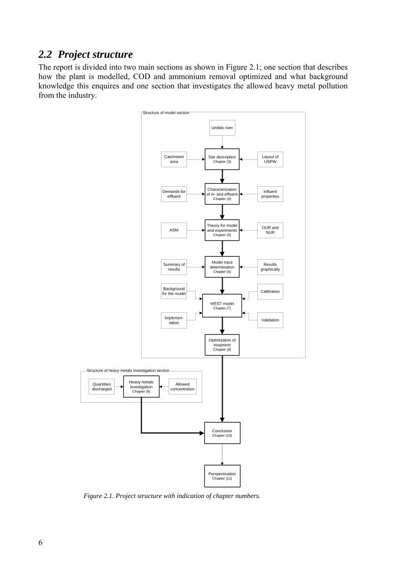
2.2 Project structure The report is divided into two main sections as shown in Figure 2.1; one section that describes how the plant is modelled, COD and ammonium removal optimized and what background knowledge this enquires and one section that investigates the allowed heavy metal pollution from the industry.

Site descriptionChapter (3)

Influentproperties

WEST modelChapter (7)

Backgroundfor the model

Validation

Calibration

Implemen-tation

Heavy metalsinvestigation

Chapter (9)

ConclusionChapter (10)

Characterizationof in- and effluent

Chapter (4)

Optimization oftreatmentChapter (8)

Demands foreffluent

Layout ofUSPW

Catchmentarea

Umbilo river

Allowedconcentration

Quantitiesdischarged

PerspectivationChapter (11)

Structure of model section

Structure of heavy metals investigation section

Theory for modeland experiments

Chapter (5)

Model inputdetermination

Chapter (6)

Summary ofresults

Resultsgraphically

ASM OUR andNUR

Figure 2.1. Project structure with indication of chapter numbers.

6

In Figure 2.1 is the project structure with chapters shown and a brief introduction to each chapter will be given in the following. Chapter 3 – This chapter introduces the location of the catchment area, Umbilo river and

USPW in DMA. In the subsection “The catchment area” are the sewer network and industries of relevance described. In “Umbilo river” are the source and course of the river illustrated. “Layout of USPW” describes the modelled part of the plant, i.e. the new works. The old works along with the anaerobic digesters are also described partly to give an overview of the entire plant and partly because they are used to estimate relevant flows at USPW for the modelling purpose.

Chapter 4 – This chapter characterises the raw sewage by assessment of dynamics and

irregularities in the flow volumes and a description of the composition. The characterisation of the raw sewage is important, because the characterisation is used to assess the environmental input conditions for the model. Furthermore concentrations of constituents in the effluent from both works are used to evaluate the performance of the present plant configuration by the frequency the standard are meet.

Chapter 5 – The model for optimizing the COD and ammonium removal in the continuously

stirred reactor (CSTR) is chosen as a modification of the activated sludge model No. 2. The mathematical description of the relevant treatment processes in the CSTR model is presented in a matrix notation. The procedure for determination of components and parameters making the model specific for the CSTR at USPW is described at the end of the section.

Chapter 6 – This chapter presents the results of the performed experiments graphically and

summons the values for the specific components and parameters. The values are finally compared with default values from the activated sludge model No. 2.

Chapter 7 – The WEST model is introduced with the theoretical basis and calculation solution

procedures. It is shown how the configuration of the new works is implemented in the WEST program and what sub models that are used for the single treatment units. The parameters in the model are calibrated after the three measured variables in the effluent for 2003; COD, ammonium and nitrate. The calibrated model is validated on measurements for the same variables in 2004

Chapter 8 – The calibrated and validated model are used to reduce the effluent concentration

of COD and ammonium. 5 different scenarios assess the highest possible reduction. One scenario, where the oxygen concentration in the CSTR is raised, gives the highest reduction in both COD and ammonium.

Chapter 9 – The heavy metals content in the sludge are above the maximum concentrations

for agricultural purposes. The chapter discusses the reduction from industrial effluent, which has to be made in order for USPW to dispose of the sludge for agricultural purposes. A mass balance is used to assess the necessary reduction from the industry.

7

Chapter 10 – The chapter states the recommendation for the new works, which ought to be implemented in order to reduce the COD and ammonium load to Umbilo river, based on the optimization. The maximum allowed concentration of heavy metals in the industrial effluent, where the sludge can be used for agricultural purposes, are also concluded.

Chapter 11 – This chapter lists the recommendation, which improves the model’s prediction

of different variables in the effluent. The recommendations are addressed to Durban Metropolitan, the University of KwaZulu-Natal and Umbilo Sewage Purification Works.

8

3 Site description Durban Metropolitan Area is located in the KwaZulu-Natal region in the Eastern part of South Africa. The catchment area for Umbilo Sewage Purification Works and the plant itself are located in Pinetown, one of the suburbs of Durban. The plant discharges to the Umbilo river running through the catchment area as shown in Figure 3.1.

Figure 3.1. Durban Metropolitan Area, where the catchment area for Umbilo Sewage Purification Works, the wastewater treatment plant itself, USPW, and the receiving body of water, Umbilo river, are depicted. [www.uyaphi.com, 2005]

3.1 Catchment area of Umbilo Sewage Purification Works The catchment area for USPW is app. 10 km2 and consists mostly of residential areas with a few large factories. The sewer system is divided into two separate networks; one network carries rainwater and run off from the streets and the other carries domestic and industrial effluent. The network with the rainwater gets diverted into the rivers or runs directly into the ocean without any preliminary treatment. The age of the sewer system varies ranging from 1965 to recent time, but which part of the catchments area is of recent time and which part dates back to the beginning of the sewer system is unknown. Lack of revenue might give problems in the future due to in- and exfiltration, because there are no funds to maintain the sewer system. The distance from the water consumer to USPW varies in length from 10 km and down to a few hundred meters where much of the flow is due solely to gravity. The retention time in the

9

sewer system is not known, but is estimated to range from a few minutes up to several hours. [Pers.Com. Fennemore, 2004] The microbiological processes in the sewer can have an impact on the composition of the raw sewage entering USPW. With the present knowledge of the catchment area, which is stated above, it is not possible to predict the microbiological processes in the sewer and the fate of the sewage composition. It is assessed, that the microbiological processes in the sewer system are not of vital importance, because measurements on the raw sewage right before the inlet to USPW are performed. Further investigation of the sewer system will therefore not be conducted.

3.1.1 Companies in the catchment area There are two types of industry in the catchment area, which makes up the main portion of the industrial effluent – textile and metal finishing companies. Following industries in the area can have a significant impact on the industrial effluents, hence affect the performance of USPW;

- Two larger textile companies - One company, which stores mostly dyes - One printing company - Two larger metal finishing companies

[Pers.Com. Fennemore, 2004] The authors do not have access to the discharge concentrations and volumes from the companies in the catchment area, because this information is confidential. Nor the exact number of textile and metal finishing companies in the area, or the received amount of effluent from the two types of industries are known, due to small backyard companies not registered at the municipality. [Pers.Com. Fennemore, 2004]

10

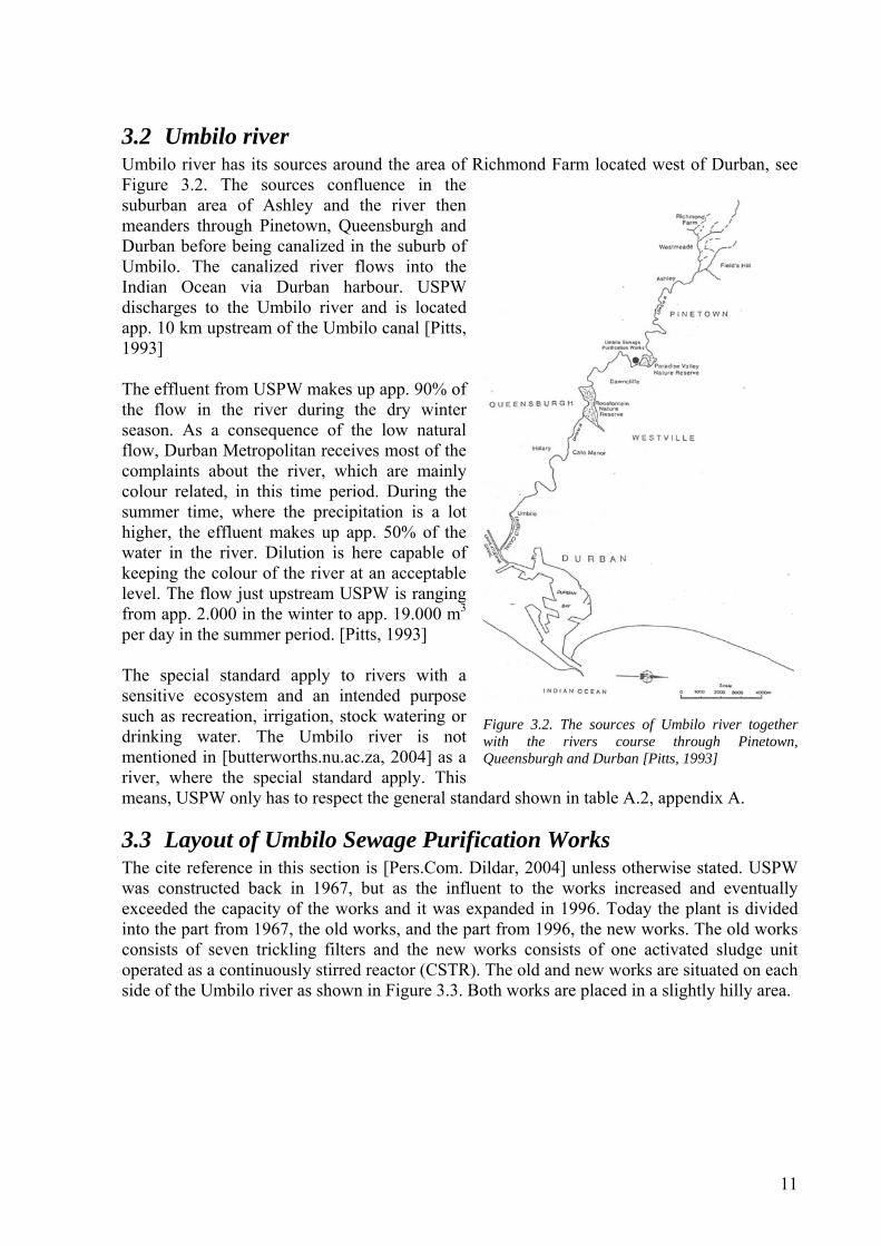
3.2 Umbilo river Umbilo river has its sources around the area of Richmond Farm located west of Durban, see Figure 3.2. The sources confluence in the suburban area of Ashley and the river then meanders through Pinetown, Queensburgh and Durban before being canalized in the suburb of Umbilo. The canalized river flows into the Indian Ocean via Durban harbour. USPW discharges to the Umbilo river and is located app. 10 km upstream of the Umbilo canal [Pitts, 1993] The effluent from USPW makes up app. 90% of the flow in the river during the dry winter season. As a consequence of the low natural flow, Durban Metropolitan receives most of the complaints about the river, which are mainly colour related, in this time period. During the summer time, where the precipitation is a lot higher, the effluent makes up app. 50% of the water in the river. Dilution is here capable of keeping the colour of the river at an acceptable level. The flow just upstream USPW is ranging from app. 2.000 in the winter to app. 19.000 m3 per day in the summer period. [Pitts, 1993] The special standard apply to rivers with a sensitive ecosystem and an intended purpose such as recreation, irrigation, stock watering or drinking water. The Umbilo river is not mentioned in [butterworths.nu.ac.za, 2004] as a river, where the special standard apply. This means, USPW only has to respect the general standard shown in table A.2, appendix A.

Figure 3.2. The sources of Umbilo river together with the rivers course through Pinetown, Queensburgh and Durban [Pitts, 1993]

3.3 Layout of Umbilo Sewage Purification Works The cite reference in this section is [Pers.Com. Dildar, 2004] unless otherwise stated. USPW was constructed back in 1967, but as the influent to the works increased and eventually exceeded the capacity of the works and it was expanded in 1996. Today the plant is divided into the part from 1967, the old works, and the part from 1996, the new works. The old works consists of seven trickling filters and the new works consists of one activated sludge unit operated as a continuously stirred reactor (CSTR). The old and new works are situated on each side of the Umbilo river as shown in Figure 3.3. Both works are placed in a slightly hilly area.

11

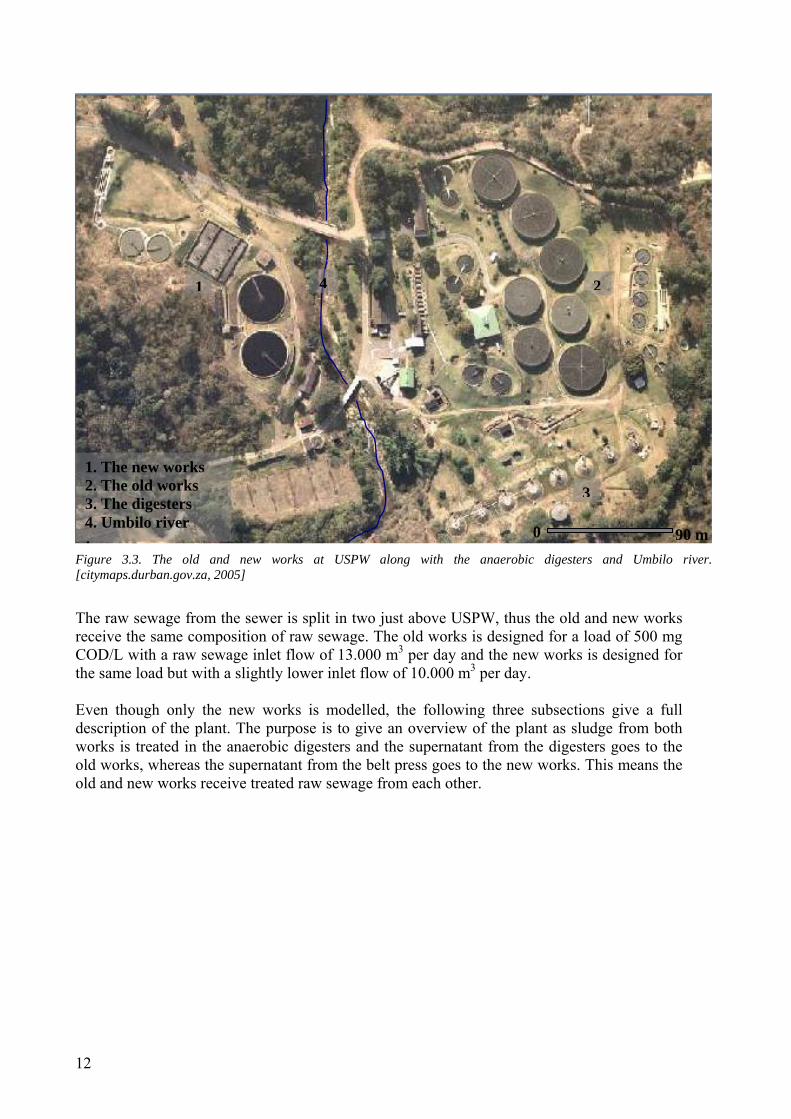
1. The new works 2. The old works 3. The digesters 4. Umbilo river

1 2

3

4

0 90 m Figure 3.3. The old and new works at USPW along with the anaerobic digesters and Umbilo river. [citymaps.durban.gov.za, 2005]

The raw sewage from the sewer is split in two just above USPW, thus the old and new works receive the same composition of raw sewage. The old works is designed for a load of 500 mg COD/L with a raw sewage inlet flow of 13.000 m3 per day and the new works is designed for the same load but with a slightly lower inlet flow of 10.000 m3 per day. Even though only the new works is modelled, the following three subsections give a full description of the plant. The purpose is to give an overview of the plant as sludge from both works is treated in the anaerobic digesters and the supernatant from the digesters goes to the old works, whereas the supernatant from the belt press goes to the new works. This means the old and new works receive treated raw sewage from each other.

12

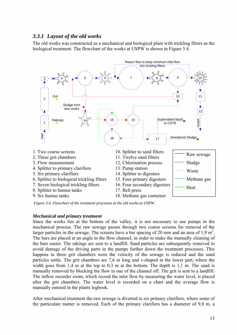
3.3.1 Layout of the old works The old works was constructed as a mechanical and biological plant with trickling filters as the biological treatment. The flowchart of the works at USPW is shown in Figure 3.4.

3 5 74 6 9

11

12

Inle

t

Out

let

13

1

2

8

Rakings

Grit

15

18 17 Dewatered Sludge

14

10

Sludge fromnew works

16 Supernatant liquidto CSTR

Return flow to keep minimum inlet flowinto trickling filters

1. Two coarse screens 10. Splitter to sand filters 2. Three grit chambers 11. Twelve sand filters 3. Flow measurement 12. Chlorination process 4. Splitter to primary clarifiers 13. Pump station 5. Six primary clarifiers 14. Splitter to digesters 6. Splitter to biological trickling filters 15. Four primary digesters 7. Seven biological trickling filters 16. Four secondary digesters 8. Splitter to humus tanks 17. Belt press 9. Six humus tanks 18. Methane gas container Figure 3.4. Flowchart of the treatment processes at the old works at USPW.

Raw sewage

Sludge

Waste

Methane gas

Heat

Mechanical and primary treatment Since the works lies at the bottom of the valley, it is not necessary to use pumps in the mechanical process. The raw sewage passes through two coarse screens for removal of the larger particles in the sewage. The screens have a bar spacing of 20 mm and an area of 1,9 m2. The bars are placed at an angle in the flow channel, in order to make the manually cleaning of the bars easier. The rakings are sent to a landfill. Sand particles are subsequently removed to avoid damage of the driving parts in the pumps further down the treatment processes. This happens in three grit chambers were the velocity of the sewage is reduced and the sand particles settle. The grit chambers are 7,6 m long and v-shaped in the lower part, where the width goes from 1,4 m at the top to 0,3 m at the bottom. The depth is 1,1 m. The sand is manually removed by blocking the flow in one of the channel off. The grit is sent to a landfill. The inflow recorder room, which record the inlet flow by measuring the water level, is placed after the grit chambers. The water level is recorded on a chart and the average flow is manually entered in the plants logbook. After mechanical treatment the raw sewage is diverted to six primary clarifiers, where some of the particulate matter is removed. Each of the primary clarifiers has a diameter of 9,8 m, a

13

surface area of 75 m2 and a volume of 227 m3, which gives a retention time of 2½ hours at the design flow rate. The clarifiers are manually desludged twice a day. Biological treatment with trickling filters The sewage is pumped to the top of seven biological trickling filters, where the force of the water flow causes sprinklers to turn, hence distributing the sewage evenly over the surface of the trickling filters. There is a return flow from the effluent of the humus tanks to maintain a minimum flow into the trickling filters to keep the sprinklers turning. The filters consist of crushed stone with a large surface area. On the surface of the crushed stones a biofilm growth, where bacteria transform the soluble matter into particulate matter. This continues until the film becomes too thick and the force of the flowing water rips chunks off. The biofilm consists of zones with different electron acceptors according to the thickness of the film. At the very edge of the biofilm, where the film is in contact with the aerated raw sewage, exists an aerobic zone. As the raw sewage penetrates further into the biofilm, oxygen is depleted and the zone changes to an anoxic zone and finally an anaerobic zone, when nitrate is depleted. In the aerobic zone nitrification happens, where ammonia is oxidized to nitrite and subsequently to nitrate. Denitrification occurs in the anoxic zone, where nitrate is used as electron acceptor and reduced to atmospheric nitrogen. [Tchobanoglous et al., 2003] The seven trickling filters have two different diameters with three at 26,5 meters and four at 33,2 meters and a height of all filters at 4,3 meters. There is no explanation of the two different diameters. Secondary and tertiary treatment The sewage flows via gravity to six humus tanks, where the particular matter settles. Subsequently the particular matter is pumped back to the primary clarifiers. The humus tanks have a diameter of 13,5 meters, a surface area of 140 m2 and a volume of 300 m3 for each tank, which gives a retention time of about 3½ hours at the design flow rate. The treated sewage is diverted to twelve gravitation sand filters, where the sand filters remove smaller particles not removed in the humus tanks. The total surface area of the twelve sand filters are 11,6 m2 with a filtering capacity of 7,3 m3/(m2⋅hr) or a flow of 24.500 m3 per day of treated effluent. The sand filters are manually operated and backwashed. The tertiary treatment before the wastewater is discharged to Umbilo river is chlorination, where chlorine gas is injected into the water. The purpose is to kill any pathogenic organisms that might be in the wastewater.

14

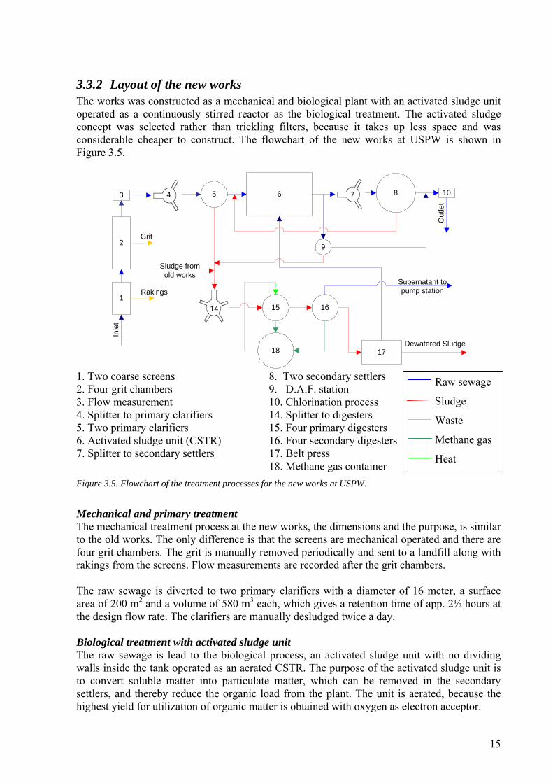
3.3.2 Layout of the new works The works was constructed as a mechanical and biological plant with an activated sludge unit operated as a continuously stirred reactor as the biological treatment. The activated sludge concept was selected rather than trickling filters, because it takes up less space and was considerable cheaper to construct. The flowchart of the new works at USPW is shown in Figure 3.5.

3 4

Inle

t

1

2

Rakings

Grit

5 6 8

9

107

Out

let

14

Sludge fromold works

15

18 17Dewatered Sludge

16

Supernatant topump station

1. Two coarse screens 8. Two secondary settlers 2. Four grit chambers 9. D.A.F. station 3. Flow measurement 10. Chlorination process 4. Splitter to primary clarifiers 14. Splitter to digesters 5. Two primary clarifiers 15. Four primary digesters 6. Activated sludge unit (CSTR) 16. Four secondary digesters 7. Splitter to secondary settlers 17. Belt press 18. Methane gas container Figure 3.5. Flowchart of the treatment processes for the new works at USPW.

Raw sewage

Sludge

Waste

Methane gas

Heat

Mechanical and primary treatment The mechanical treatment process at the new works, the dimensions and the purpose, is similar to the old works. The only difference is that the screens are mechanical operated and there are four grit chambers. The grit is manually removed periodically and sent to a landfill along with rakings from the screens. Flow measurements are recorded after the grit chambers. The raw sewage is diverted to two primary clarifiers with a diameter of 16 meter, a surface area of 200 m2 and a volume of 580 m3 each, which gives a retention time of app. 2½ hours at the design flow rate. The clarifiers are manually desludged twice a day. Biological treatment with activated sludge unit The raw sewage is lead to the biological process, an activated sludge unit with no dividing walls inside the tank operated as an aerated CSTR. The purpose of the activated sludge unit is to convert soluble matter into particulate matter, which can be removed in the secondary settlers, and thereby reduce the organic load from the plant. The unit is aerated, because the highest yield for utilization of organic matter is obtained with oxygen as electron acceptor.

15

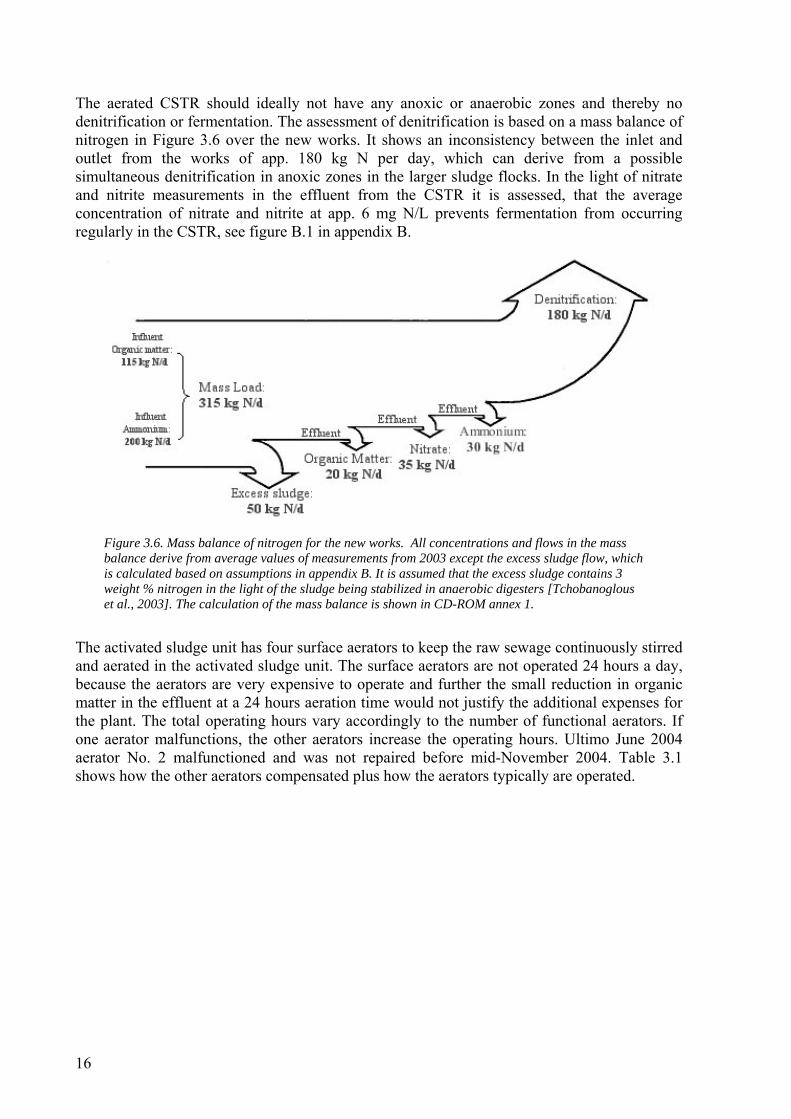
The aerated CSTR should ideally not have any anoxic or anaerobic zones and thereby no denitrification or fermentation. The assessment of denitrification is based on a mass balance of nitrogen in Figure 3.6 over the new works. It shows an inconsistency between the inlet and outlet from the works of app. 180 kg N per day, which can derive from a possible simultaneous denitrification in anoxic zones in the larger sludge flocks. In the light of nitrate and nitrite measurements in the effluent from the CSTR it is assessed, that the average concentration of nitrate and nitrite at app. 6 mg N/L prevents fermentation from occurring regularly in the CSTR, see figure B.1 in appendix B.

Figure 3.6. Mass balance of nitrogen for the new works. All concentrations and flows in the mass balance derive from average values of measurements from 2003 except the excess sludge flow, which is calculated based on assumptions in appendix B. It is assumed that the excess sludge contains 3 weight % nitrogen in the light of the sludge being stabilized in anaerobic digesters [Tchobanoglous et al., 2003]. The calculation of the mass balance is shown in CD-ROM annex 1.

The activated sludge unit has four surface aerators to keep the raw sewage continuously stirred and aerated in the activated sludge unit. The surface aerators are not operated 24 hours a day, because the aerators are very expensive to operate and further the small reduction in organic matter in the effluent at a 24 hours aeration time would not justify the additional expenses for the plant. The total operating hours vary accordingly to the number of functional aerators. If one aerator malfunctions, the other aerators increase the operating hours. Ultimo June 2004 aerator No. 2 malfunctioned and was not repaired before mid-November 2004. Table 3.1 shows how the other aerators compensated plus how the aerators typically are operated.

16

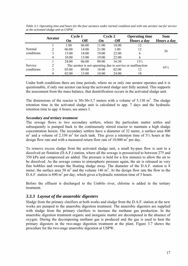
Table 3.1. Operating time and hours for the four aerators under normal condition and with one aerator out for service at the activated sludge unit at USPW.

Cycle 1 Cycle 2 Operating time Sum Aerator On Off On Off Hours a day Hours a day

1 1:00 06:00 11:00 18:00 12 2 06:00 14:00 21:00 1:00 12 3 15:00 18:00 19:00 22:00 6

Normal conditions

4 10:00 13:00 19:00 22:00 6

36

1 24:00 06:00 09:00 16:30 13½ 2 The aerator is not operating due to service or malfunction 3 05:00 09:00 18:00 02:00 12

Service conditions

4 02:00 13:00 18:00 24:00 18

43½

Under both conditions there are time periods, where no or only one aerator operates and it is questionable, if only one aerator can keep the activated sludge unit fully aerated. This supports the assessment from the mass balance, that denitrification occurs in the activated sludge unit. The dimensions of the reactor is 30×30×5,7 meters with a volume of 5.130 m3. The sludge retention time in the activated sludge unit is calculated to app. 7 days and the hydraulic retention time to app. 6 hours, see annex I. Secondary and tertiary treatment The sewage flows to two secondary settlers, where the particulate matter settles and subsequently is pumped back to the continuously stirred reactor to maintain a high sludge concentration herein. The secondary settlers have a diameter of 32 meter, a surface area 800 m2 and a volume of 2.330 m3 for each tank. This gives a retention time of 5½ hours at the design flow rate and with a measured return flow rate of 10.000 m3 per day. To remove excess sludge from the activated sludge unit, a small by-pass flow is sent to a dissolved air flotation (D.A.F.) station, where all the sewage is pressurized to between 275 and 350 kPa and compressed air added. The pressure is held for a few minutes to allow the air to be dissolved. As the sewage comes to atmospheric pressure again, the air is released as very fine bobbles and sweeps the floating sludge away. The diameter of the D.A.F. station is 8 meter, the surface area 50 m2 and the volume 146 m3. At the design flow rate the flow to the D.A.F. station is 690 m3 per day, which gives a hydraulic retention time of 5 hours. Before the effluent is discharged to the Umbilo river, chlorine is added in the tertiary treatment.

3.3.3 Layout of the anaerobic digesters Sludge from the primary clarifiers at both works and sludge from the D.A.F. station at the new works are pumped to the anaerobic digestion treatment. The anaerobic digesters are supplied with sludge from the primary clarifiers to increase the methane gas production. In the anaerobic digestion treatment organic and inorganic matter are decomposed in the absence of oxygen. During the decomposing methane gas is produced and the gas is used to heat the primary digesters in the two-stage digestion treatment at the plant. Figure 3.7 shows the procedure for the two-stage anaerobic digestion at USPW.

17

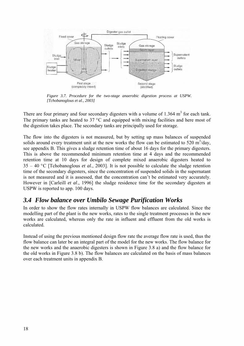
Figure 3.7. Procedure for the two-stage anaerobic digestion process at USPW. [Tchobanoglous et al., 2003]

There are four primary and four secondary digesters with a volume of 1.364 m3 for each tank. The primary tanks are heated to 37 °C and equipped with mixing facilities and here most of the digestion takes place. The secondary tanks are principally used for storage. The flow into the digesters is not measured, but by setting up mass balances of suspended solids around every treatment unit at the new works the flow can be estimated to 520 m3/day, see appendix B. This gives a sludge retention time of about 16 days for the primary digesters. This is above the recommended minimum retention time at 4 days and the recommended retention time at 10 days for design of complete mixed anaerobic digesters heated to 35 – 40 °C [Tchobanoglous et al., 2003]. It is not possible to calculate the sludge retention time of the secondary digesters, since the concentration of suspended solids in the supernatant is not measured and it is assessed, that the concentration can’t be estimated very accurately. However in [Carleill et al., 1996] the sludge residence time for the secondary digesters at USPW is reported to app. 100 days.

3.4 Flow balance over Umbilo Sewage Purification Works In order to show the flow rates internally in USPW flow balances are calculated. Since the modelling part of the plant is the new works, rates to the single treatment processes in the new works are calculated, whereas only the rate in influent and effluent from the old works is calculated. Instead of using the previous mentioned design flow rate the average flow rate is used, thus the flow balance can later be an integral part of the model for the new works. The flow balance for the new works and the anaerobic digesters is shown in Figure 3.8 a) and the flow balance for the old works in Figure 3.8 b). The flow balances are calculated on the basis of mass balances over each treatment units in appendix B.

18

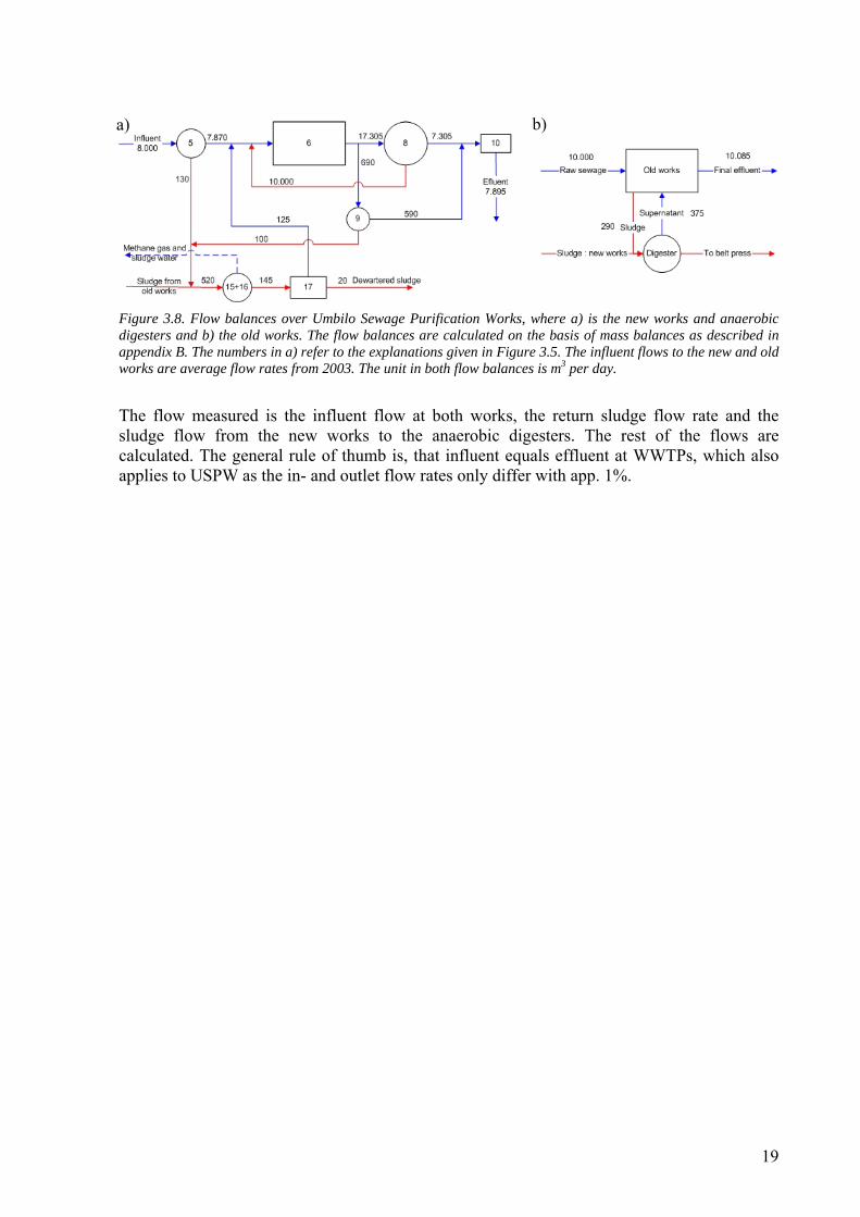
Figure 3.8. Flow balances over Umbilo Sewage Purification Works, where a) is the new works and anaerobic digesters and b) the old works. The flow balances are calculated on the basis of mass balances as described in appendix B. The numbers in a) refer to the explanations given in Figure 3.5. The influent flows to the new and old works are average flow rates from 2003. The unit in both flow balances is m3 per day.

The flow measured is the influent flow at both works, the return sludge flow rate and the sludge flow from the new works to the anaerobic digesters. The rest of the flows are calculated. The general rule of thumb is, that influent equals effluent at WWTPs, which also applies to USPW as the in- and outlet flow rates only differ with app. 1%.

b) a)

19

4 Characterisation of influent and effluent This chapter describes the influent of volumes and specific components to Umbilo Sewage Purification Works and illustrates the loads and fluctuations. It also documents the efficiency of the present plant configuration by assessing, how often the general standard for the effluent is met. Measurements of the incoming wastewater to USPW are available from January 1999 for the flow and January 2000 for the remaining chemical data and until October 2004. Chemical data are digitally drawn from the Laboratory Information System (LIMS) at Durban Metropolitan and flow data are manually collected from USPW’s data logbook. The chemical data set is collected in CD-ROM annex 1 and the data set for flow in CD-ROM annex 2.

4.1 Influent characterisation In the light of the collected dataset this section describes the incoming wastewater by an interpretation of the incoming volumes and a review of the composition.

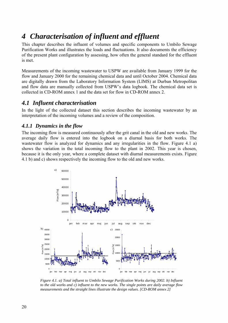
4.1.1 Dynamics in the flow The incoming flow is measured continuously after the grit canal in the old and new works. The average daily flow is entered into the logbook on a diurnal basis for both works. The wastewater flow is analyzed for dynamics and any irregularities in the flow. Figure 4.1 a) shows the variation in the total incoming flow to the plant in 2002. This year is chosen, because it is the only year, where a complete dataset with diurnal measurements exists. Figure 4.1 b) and c) shows respectively the incoming flow to the old and new works.

0

10000

20000

30000

40000

50000

60000

jan feb m ar apr maj jun jul aug sep okt nov dec

Flow

[m3 /

d]

0

5000

10000

15000

20000

25000

30000

35000

40000

jan feb mar apr maj jun jul aug sep okt nov dec

Flow

[m3 /d

]

0

5000

10000

15000

20000

25000

jan feb mar apr maj jun jul aug sep okt nov dec

Flow

[m3 /d

]

a)

b) c)

Figure 4.1. a) Total influent to Umbilo Sewage Purification Works during 2002. b) Influent to the old works and c) influent to the new works. The single points are daily average flow measurements and the straight lines illustrate the design values. [CD-ROM annex 2]

20

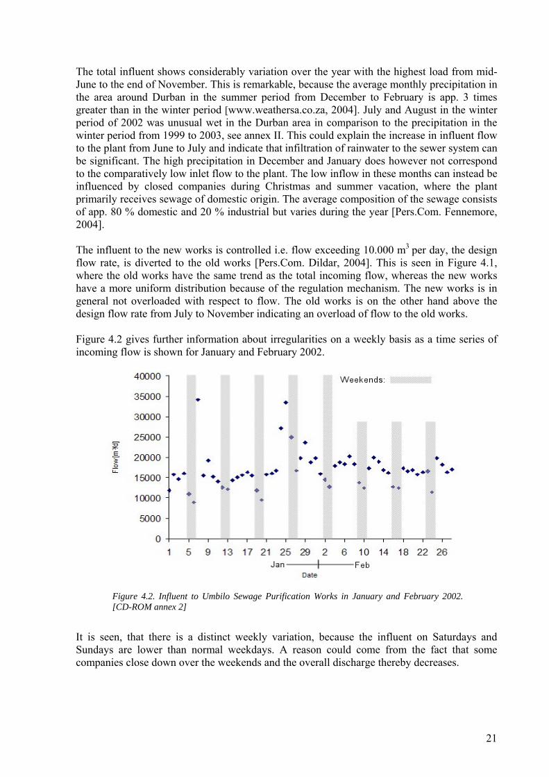
The total influent shows considerably variation over the year with the highest load from mid-June to the end of November. This is remarkable, because the average monthly precipitation in the area around Durban in the summer period from December to February is app. 3 times greater than in the winter period [www.weathersa.co.za, 2004]. July and August in the winter period of 2002 was unusual wet in the Durban area in comparison to the precipitation in the winter period from 1999 to 2003, see annex II. This could explain the increase in influent flow to the plant from June to July and indicate that infiltration of rainwater to the sewer system can be significant. The high precipitation in December and January does however not correspond to the comparatively low inlet flow to the plant. The low inflow in these months can instead be influenced by closed companies during Christmas and summer vacation, where the plant primarily receives sewage of domestic origin. The average composition of the sewage consists of app. 80 % domestic and 20 % industrial but varies during the year [Pers.Com. Fennemore, 2004]. The influent to the new works is controlled i.e. flow exceeding 10.000 m3 per day, the design flow rate, is diverted to the old works [Pers.Com. Dildar, 2004]. This is seen in Figure 4.1, where the old works have the same trend as the total incoming flow, whereas the new works have a more uniform distribution because of the regulation mechanism. The new works is in general not overloaded with respect to flow. The old works is on the other hand above the design flow rate from July to November indicating an overload of flow to the old works. Figure 4.2 gives further information about irregularities on a weekly basis as a time series of incoming flow is shown for January and February 2002.

Figure 4.2. Influent to Umbilo Sewage Purification Works in January and February 2002. [CD-ROM annex 2]

It is seen, that there is a distinct weekly variation, because the influent on Saturdays and Sundays are lower than normal weekdays. A reason could come from the fact that some companies close down over the weekends and the overall discharge thereby decreases.

21

From the information about flow dynamics and irregularities it is concluded that USPW has to deal with variation in the flow on both long and short-term basis and that the new works in general is not overloaded with respect to the flow.

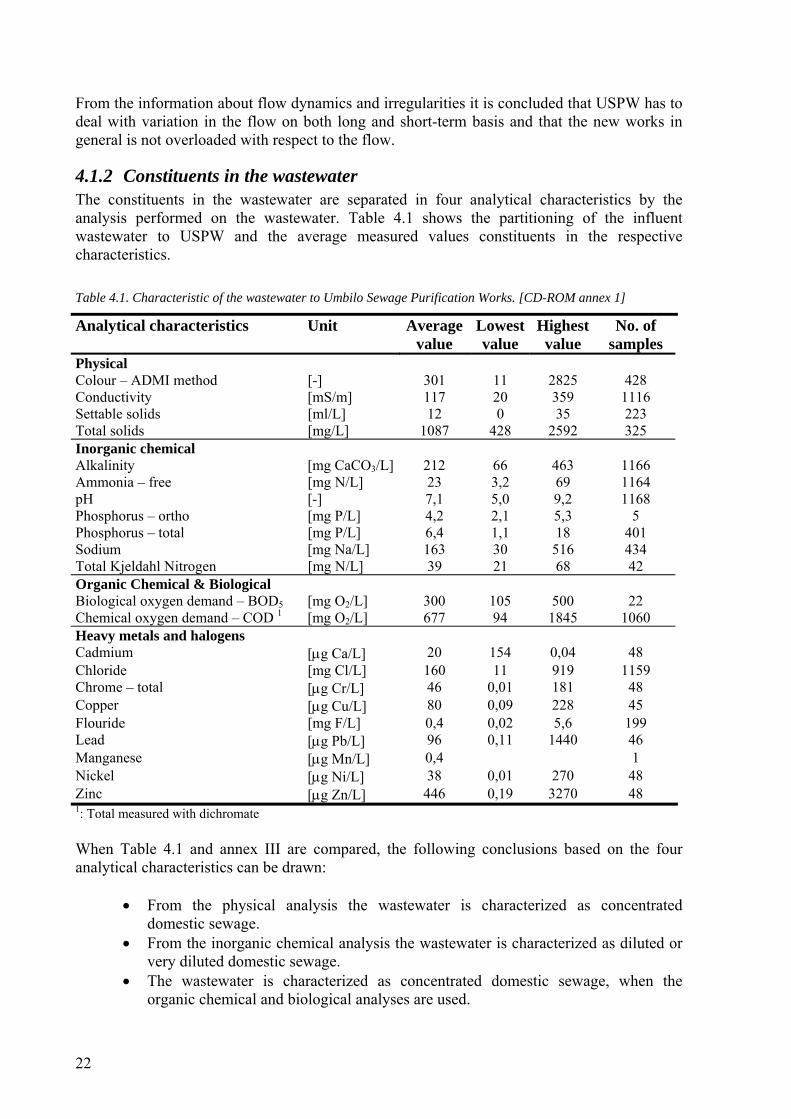
4.1.2 Constituents in the wastewater The constituents in the wastewater are separated in four analytical characteristics by the analysis performed on the wastewater. Table 4.1 shows the partitioning of the influent wastewater to USPW and the average measured values constituents in the respective characteristics. Table 4.1. Characteristic of the wastewater to Umbilo Sewage Purification Works. [CD-ROM annex 1]

Analytical characteristics Unit Average value

Lowest value

Highest value

No. of samples

Physical Colour – ADMI method [-] 301 11 2825 428 Conductivity [mS/m] 117 20 359 1116 Settable solids [ml/L] 12 0 35 223 Total solids [mg/L] 1087 428 2592 325 Inorganic chemical Alkalinity [mg CaCO3/L] 212 66 463 1166 Ammonia – free [mg N/L] 23 3,2 69 1164 pH [-] 7,1 5,0 9,2 1168 Phosphorus – ortho [mg P/L] 4,2 2,1 5,3 5 Phosphorus – total [mg P/L] 6,4 1,1 18 401 Sodium [mg Na/L] 163 30 516 434 Total Kjeldahl Nitrogen [mg N/L] 39 21 68 42 Organic Chemical & Biological Biological oxygen demand – BOD5 [mg O2/L] 300 105 500 22 Chemical oxygen demand – COD 1 [mg O2/L] 677 94 1845 1060 Heavy metals and halogens Cadmium [µg Ca/L] 20 154 0,04 48 Chloride [mg Cl/L] 160 11 919 1159 Chrome – total [µg Cr/L] 46 0,01 181 48 Copper [µg Cu/L] 80 0,09 228 45 Flouride [mg F/L] 0,4 0,02 5,6 199 Lead [µg Pb/L] 96 0,11 1440 46 Manganese [µg Mn/L] 0,4 1 Nickel [µg Ni/L] 38 0,01 270 48 Zinc [µg Zn/L] 446 0,19 3270 48 1: Total measured with dichromate When Table 4.1 and annex III are compared, the following conclusions based on the four analytical characteristics can be drawn:

• From the physical analysis the wastewater is characterized as concentrated domestic sewage.

• From the inorganic chemical analysis the wastewater is characterized as diluted or very diluted domestic sewage.

• The wastewater is characterized as concentrated domestic sewage, when the organic chemical and biological analyses are used.

22

• The heavy metals measurements characterize the wastewater as concentrated domestic sewage, whereas the characterization based on the halogens describes the wastewater as very diluted domestic sewage.

It is not possible to distinctively characterize the wastewater based on an overall assessment of the four analyses. Instead the characterisation is based on central ratio relationships, such as COD/BOD and COD/TN, and threshold concentrations of heavy metals. The COD/BOD ratio states, how readily biodegradable the wastewater is, i.e. the lower ratio the more readily biodegradable wastewater, with 2 – 2,5 being typical values [Henze et al., 2002]. The ratio for the inlet to USPW is about 2, which indicates a normal potential for biodegrading the wastewater. The COD/TN ratio affects the denitrification process, as it indicates the amount of substrate available for the biomass to perform denitrification. A high ratio, 10 – 14 kg COD/kg TN, provides the possibility of a fast denitrification process, whereas with a low ratio, 6 – 10 kg COD/kg TN, the process becomes slow and extern carbon-source might be needed, if the process is to succeed [Winther et al., 1998]. The COD/TN ratio for Umbilo is calculated to 17 and this means that the carbon content in the sewage is sufficient for maintaining a denitrification process under anoxic condition. The threshold concentration for heavy metals indicates the concentration at which the heavy metals exert an inhibitory effect on growth of the biomass, see annex IV. The concentration of the heavy metals in the raw sewage does not exceed the threshold concentration for heterotrophic organisms and a significant inhibitory effect from the heavy metals on the heterotrophic organisms growth can therefore not be expected in the plant assuming that no accumulation take place [Tchobanoglous et al., 2003]. The threshold concentration on the growth of autotrophic organisms is not known, but since they have a slower growth rate than heterotrophic organisms and therefore more sensitive to changes in their environment, the heavy metal concentration in the raw sewage might have an inhibitory effect on the autotrophic organism. What these conditions in the influent entail for the performance of the plant is in the following assessed by evaluating, how often the effluent complies with the legislation.

4.2 Discharge demands for effluent The old works at USPW has to comply with the general standard from the water act of 1956 according to the status of the Umbilo river, but has relaxation on three of the components from the standard as shown in Table 4.2. Table 4.2. The old works at USPW has relaxation from three specific components in the Water Act No. 54 of 1956. [Pers.Com. Howarth, 2005]

Component Unit General standard USPW relaxation COD [mg/L] 75 120 Electrical Conductivity [mS/m] 90 200 Sodium [mg/L] 75 250 The old works has to comply with the general standard for the rest of the 25 discharge components as shown in table A.1 in appendix A and the discharge demands for all the

23

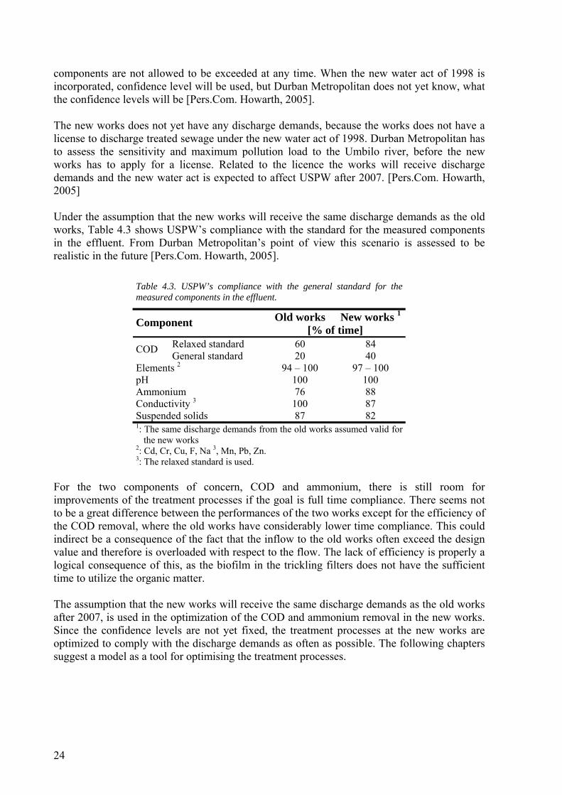
components are not allowed to be exceeded at any time. When the new water act of 1998 is incorporated, confidence level will be used, but Durban Metropolitan does not yet know, what the confidence levels will be [Pers.Com. Howarth, 2005]. The new works does not yet have any discharge demands, because the works does not have a license to discharge treated sewage under the new water act of 1998. Durban Metropolitan has to assess the sensitivity and maximum pollution load to the Umbilo river, before the new works has to apply for a license. Related to the licence the works will receive discharge demands and the new water act is expected to affect USPW after 2007. [Pers.Com. Howarth, 2005] Under the assumption that the new works will receive the same discharge demands as the old works, Table 4.3 shows USPW’s compliance with the standard for the measured components in the effluent. From Durban Metropolitan’s point of view this scenario is assessed to be realistic in the future [Pers.Com. Howarth, 2005].

Table 4.3. USPW’s compliance with the general standard for the measured components in the effluent.

Old works New works 1Component [% of time]

Relaxed standard 60 84 COD General standard 20 40 Elements 2 94 – 100 97 – 100 pH 100 100 Ammonium 76 88 Conductivity 3 100 87 Suspended solids 87 82 1: The same discharge demands from the old works assumed valid for

the new works 2: Cd, Cr, Cu, F, Na 3, Mn, Pb, Zn. 3: The relaxed standard is used.

For the two components of concern, COD and ammonium, there is still room for improvements of the treatment processes if the goal is full time compliance. There seems not to be a great difference between the performances of the two works except for the efficiency of the COD removal, where the old works have considerably lower time compliance. This could indirect be a consequence of the fact that the inflow to the old works often exceed the design value and therefore is overloaded with respect to the flow. The lack of efficiency is properly a logical consequence of this, as the biofilm in the trickling filters does not have the sufficient time to utilize the organic matter. The assumption that the new works will receive the same discharge demands as the old works after 2007, is used in the optimization of the COD and ammonium removal in the new works. Since the confidence levels are not yet fixed, the treatment processes at the new works are optimized to comply with the discharge demands as often as possible. The following chapters suggest a model as a tool for optimising the treatment processes.

24

5 Theory for CSTR model and experiments As the end of the previous chapter states, the COD and ammonium removal in the new works is not optimal and improvements are required in the CSTR, if the COD and ammonium concentrations in the effluent are to be reduced and thereby increase the time of complying with the general standard. Since the CSTR is an activated sludge unit an activated sludge model is considered as a useful tool for optimisations of the CSTR. This chapter introduces the activated sludge model and describe the theoretical basis for the model. In chapter 7 is the activated sludge model incorporated in the WEST program as part of the model for the new works. The activated sludge model is a general tool and to make this model specific for the CSTR at USPW, some essential COD fractions and model parameters in the model are determined. The methods and procedures to determine the model specific fractions and parameters are presented later in the chapter.

5.1 Activated sludge model The first Activated Sludge Model (ASM1) was introduced by IAWQ Task Group on Mathematical Modelling for Design and Operation of Biological Wastewater Treatment Process in 1987. Later several extensions of ASM1, to improve the mathematical description of the biological processes in the system, have been published. In 1995 came the extension Activated Sludge Model No. 2 (ASM2) followed by the Activated Sludge Model No. 2d (ASM2d) in 1999. The biological processes in ASM2d include some improvements compared with ASM2 on the prediction of phosphor removal and denitrification by phosphor accumulating organisms. These improvements are seen as irrelevant in this context, because the new works at USPW is not designed for biological phosphor removal. ASM2 is more complex and includes more components than the previous model, ASM1, and can model the biological processes more accurately [Henze at al., 1995]. This is why ASM2 is preferred as a basis to characterize the wastewater for the specific environment and model the CSTR at USPW. ASM2 is capable of modelling the processes;

• Removal of organic matter • Nitrification and denitrification • Fermentation • Biological phosphor removal and precipitation of phosphor

Not all the applications will be considered in this context, as the CSTR at the new works has limited possibilities included in the treatment process. The applications; fermentation, biological phosphor removal and precipitation of phosphor, are not included in the specific model compared to the original configuration of the ASM2. In the light of nitrate and nitrite measurements in the effluent from the CSTR it is assessed, that the nitrate and nitrite concentration prevents widespread fermentation in the CSTR. The phosphor accumulating organism require anaerobic condition prior to the biological treatment, under which they can store readily biodegradable substrate succeeded by aerobic or anoxic conditions, where the stored substrate is used for growth and phosphor uptake. The new works does not have this design feature implemented, thus the biological phosphor removal is eliminated. The last-mentioned application is not included in model due to the fact that no precipitant is added in the treatment process.

25

Practically the equations for fermentation, biological phosphor removal and precipitation of phosphor is still included in the CSTR model, but their influence is neglected by setting the respectively growth and rate specific constants for the processes to zero. Thus the processes are of no concern for the following CSTR model.

5.1.1 CSTR model The model for the CSTR is considered as a modification of the original ASM2. The modified model is for mathematical convenience in the following presented in a matrix notation and the nomenclature for the different components and parameters is in conformity with ASM2. Model components The matrix only considers the components, which have a significant impact on the COD-removal, nitrification and denitrification processes. Phosphorus as component is not seen as essential in this context, because phosphor exists in reasonable amounts in the influent according to Table 4.1, and is expected not to be limiting for the processes of concern. Fractions of COD and nitrogen are incorporated in the model as soluble and particulate components. Particulate constituents are given the symbol X and soluble components the symbol S. Subscription is used for specify individual components. Table 5.1 shows the components used in the CSTR model.

Table 5.1. Model components used in the CSTR model.

Unit Description Soluble components SS mg COD/L Readily biodegradable substrate SI mg COD/L Inert, non-biodegradable organics SO mg O2/L Dissolved oxygen SNO mg N/L Nitrate + Nitrit 1SN2 mg N/L Atmospheric nitrogen SNH mg N/L Ammonium SALK mole HCO3

-/L Bicarbonate alkalinity Particulate components XS mg COD/L Slowly biodegradable substrate XI mg COD/L Inert, non-biodegradable organics XH mg COD/L Heterotrophic biomass XAUT mg COD/L Autotrophic, nitrifying biomass 1: It is assumed that ammonium is transformed directly to nitrate in the nitrification process i.e. no intermediate product is included.

Model parameters In addition to the model components the model consists of a wide variety of kinetic, stoichiometric and composition parameters with constant values. The parameters are listed in Table 5.2.

26

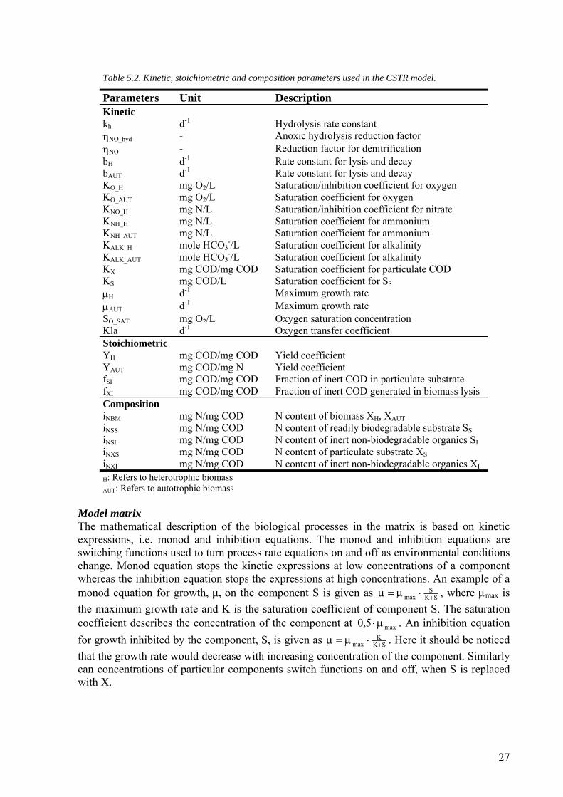
Table 5.2. Kinetic, stoichiometric and composition parameters used in the CSTR model.

Parameters Unit Description Kinetic kh d-1 Hydrolysis rate constant ηNO_hyd - Anoxic hydrolysis reduction factor ηNO - Reduction factor for denitrification bH d-1 Rate constant for lysis and decay bAUT d-1 Rate constant for lysis and decay KO_H mg O2/L Saturation/inhibition coefficient for oxygen KO_AUT mg O2/L Saturation coefficient for oxygen KNO_H mg N/L Saturation/inhibition coefficient for nitrate KNH_H mg N/L Saturation coefficient for ammonium KNH_AUT mg N/L Saturation coefficient for ammonium KALK_H mole HCO3

-/L Saturation coefficient for alkalinity KALK_AUT mole HCO3

-/L Saturation coefficient for alkalinity KX mg COD/mg COD Saturation coefficient for particulate COD KS mg COD/L Saturation coefficient for SS

µΗ d-1 Maximum growth rate µΑUT d-1 Maximum growth rate SO_SAT mg O2/L Oxygen saturation concentration Kla d-1 Oxygen transfer coefficient Stoichiometric YH mg COD/mg COD Yield coefficient YAUT mg COD/mg N Yield coefficient fSI mg COD/mg COD Fraction of inert COD in particulate substrate fXI mg COD/mg COD Fraction of inert COD generated in biomass lysis Composition iNBM mg N/mg COD N content of biomass XH, XAUTiNSS mg N/mg COD N content of readily biodegradable substrate SS iNSI mg N/mg COD N content of inert non-biodegradable organics SIiNXS mg N/mg COD N content of particulate substrate XSiNXI mg N/mg COD N content of inert non-biodegradable organics XI

H: Refers to heterotrophic biomass AUT: Refers to autotrophic biomass

Model matrix The mathematical description of the biological processes in the matrix is based on kinetic expressions, i.e. monod and inhibition equations. The monod and inhibition equations are switching functions used to turn process rate equations on and off as environmental conditions change. Monod equation stops the kinetic expressions at low concentrations of a component whereas the inhibition equation stops the expressions at high concentrations. An example of a monod equation for growth, µ, on the component S is given as SK

Smax +⋅µ=µ , where µmax is

the maximum growth rate and K is the saturation coefficient of component S. The saturation coefficient describes the concentration of the component at max5,0 µ⋅ . An inhibition equation for growth inhibited by the component, S, is given as SK

Kmax +⋅µ=µ . Here it should be noticed

that the growth rate would decrease with increasing concentration of the component. Similarly can concentrations of particular components switch functions on and off, when S is replaced with X.

27

28

input - output + reaction = accumulation

The matrix is built on the concept of mass conservation of the different components in the CSTR. Due to the fact that no mass can disappear the accumulation of mass in the CSTR is a result of equation (5.1).

(5.1) There is of cause no accumulation in a steady-state situation, because the reaction rate equals the difference between in- and output. The in- and output is physical transport of components, whereas the reaction term relies on biological utilisation or formation of components. The matrix notation makes it easier to follow the fate of the specific components as illustrated in Table 5.3.

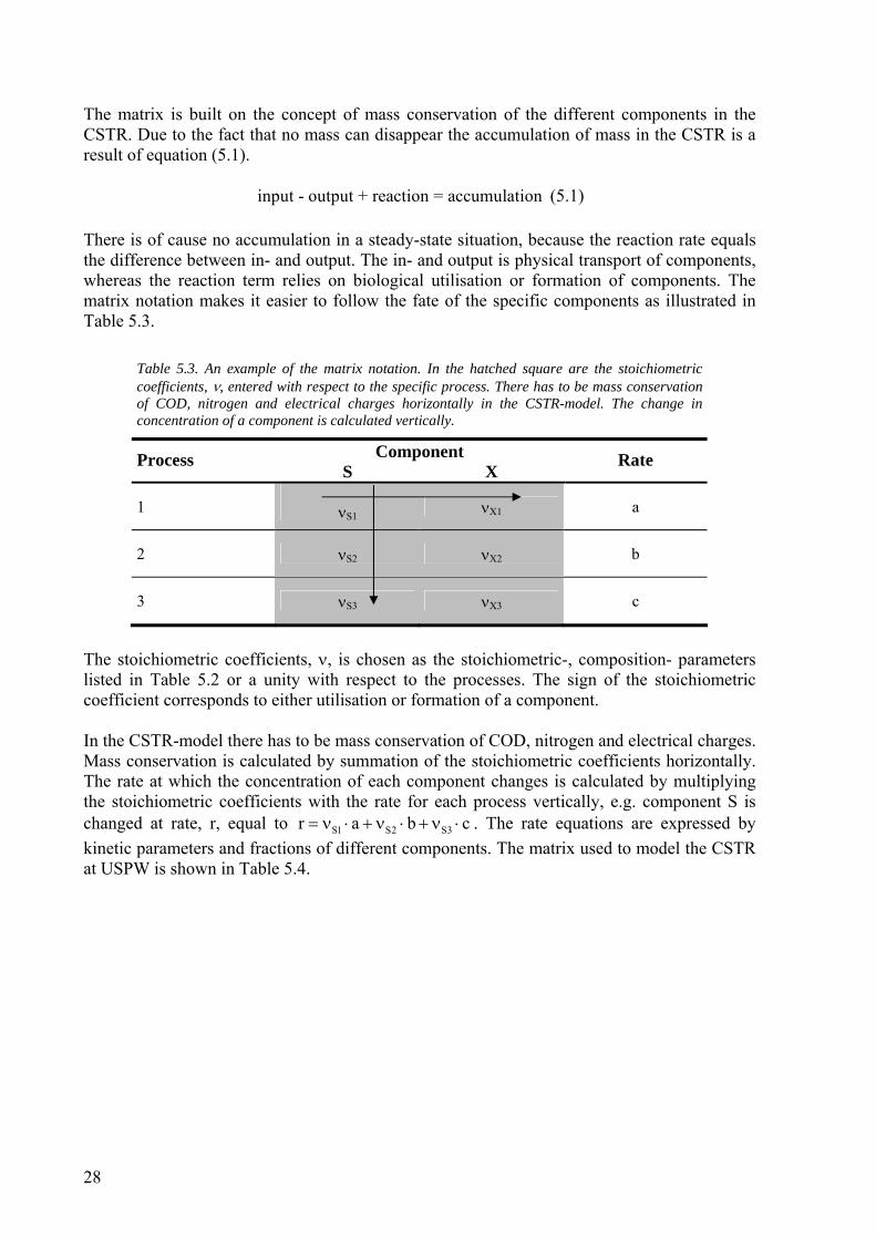
Table 5.3. An example of the matrix notation. In the hatched square are the stoichiometric coefficients, ν, entered with respect to the specific process. There has to be mass conservation of COD, nitrogen and electrical charges horizontally in the CSTR-model. The change in concentration of a component is calculated vertically.

Component Process S X

Rate

1 νS1νX1 a

2 νS2 νX2 b

3 νS3 νX3 c

The stoichiometric coefficients, ν, is chosen as the stoichiometric-, composition- parameters listed in Table 5.2 or a unity with respect to the processes. The sign of the stoichiometric coefficient corresponds to either utilisation or formation of a component. In the CSTR-model there has to be mass conservation of COD, nitrogen and electrical charges. Mass conservation is calculated by summation of the stoichiometric coefficients horizontally. The rate at which the concentration of each component changes is calculated by multiplying the stoichiometric coefficients with the rate for each process vertically, e.g. component S is changed at rate, r, equal to . The rate equations are expressed by kinetic parameters and fractions of different components. The matrix used to model the CSTR at USPW is shown in Table 5.4.

S1 S2 S3r a b c= ν ⋅ + ν ⋅ + ν ⋅

29

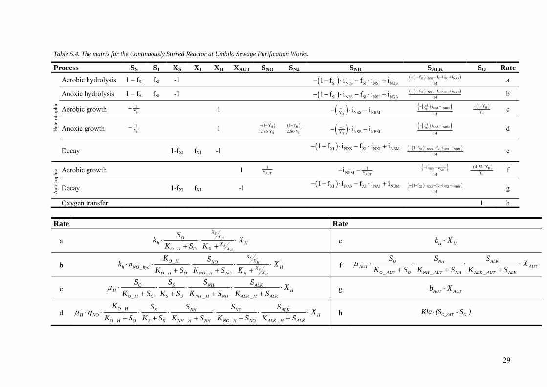
Table 5.4. The matrix for the Continuously Stirred Reactor at Umbilo Sewage Purification Works.

Process SS SI XS XI XH XAUT SNO SN2 SNH SALK SO Rate Aerobic hydrolysis 1 – fSI fSI -1 ( )SI NSS SI NSI NXS1 f i f i i− − ⋅ − ⋅ + ( )( )SI NSS SI NSI NXS1 f i f i i

14− − ⋅ − ⋅ + a

Anoxic hydrolysis 1 – fSI fSI -1 ( )SI NSS SI NSI NXS1 f i f i i− − ⋅ − ⋅ + ( )( )SI NSS SI NSI NXS1 f i f i i14

− − ⋅ − ⋅ + b

Aerobic growth H

1Y−

1 ( )H

1NSS NBMY i i−− ⋅ − ( )( )1

NSS NBMYHi i

14

−− ⋅ −

( )HY

H

1Y

− − c

Anoxic growth H

1Y− 1 ( )H

H

YY

12,86− −

⋅ ( )H

H

1 Y2,86 Y

−⋅ ( )

H

1NSS NBMY i i−− ⋅ − ( )( )1

NSS NBMYHi i

14

−− ⋅ − dH

eter

otro

phic

Decay

1-fXI fXI -1

( )XI NXS XI NXI NBM1 f i f i i− − ⋅ − ⋅ + ( )( )XI NXS XI NXI NBM1 f i f i i14

− − ⋅ − ⋅ + e

Aerobic growth 1AUT

1Y

AUT

1NBM Yi− − ( )1

NBM YAUTi

14

− −

( )H

H

4,57 YY

− − f

Aut

otro

phic

Decay

1-fXI fXI -1 ( )XI NXS XI NXI NBM1 f i f i i− − ⋅ − ⋅ + ( )( )XI NXS XI NXI NBM1 f i f i i

14− − ⋅ − ⋅ + g

Oxygen transfer 1 h Rate Rate

a _

⋅ ⋅ ⋅+ +

SH

SH

XXO

h HXXO H O X

Sk XK S K

e ⋅H Hb X

b _

__ _

⋅ ⋅ ⋅ ⋅ ⋅+ + +

SH

SH

XXO H NO

h NO hyd HXXO H O NO H NO X

K Sk XK S K S K

η f _ _ _

⋅ ⋅ ⋅ ⋅+ + +

O NH ALKAUT AUT

O AUT O NH AUT NH ALK AUT ALK

S S S XK S K S K S

µ

c _ _ _

⋅ ⋅ ⋅ ⋅ ⋅+ + + +

O S NH ALKH H

O H O S S NH H NH ALK H ALK

S S S S XK S K S K S K S

µ g ⋅AUT AUTb X

d _

_ _ _ _

⋅ ⋅ ⋅ ⋅ ⋅ ⋅ ⋅+ + + + +

O H S NH NO ALKH NO H

O H O S S NH H NH NO H NO ALK H ALK

K S S S S XK S K S K S K S K S

µ η h ⋅ O_SAT OKla (S - S )

An accurate simulation of biological processes in the CSTR based on rate equations requires specific values of the kinetic parameters and components valid for the current wastewater composition and sludge in use in the CSTR.

5.2 Methods and procedures to determine model input It is desirable that soluble and particulate components of the wastewater are included in the modelling process and that these values are specific for the raw incoming sewage and the sludge inside the CSTR. The components and parameters in focus are fractions of COD in the influent plus kinetic and stoichiometric parameters in the ASU. COD fractions gives vital information about how readily biodegradable the sewage in general is and kinetic and stoichiometric parameters control the rate of the biological processes.

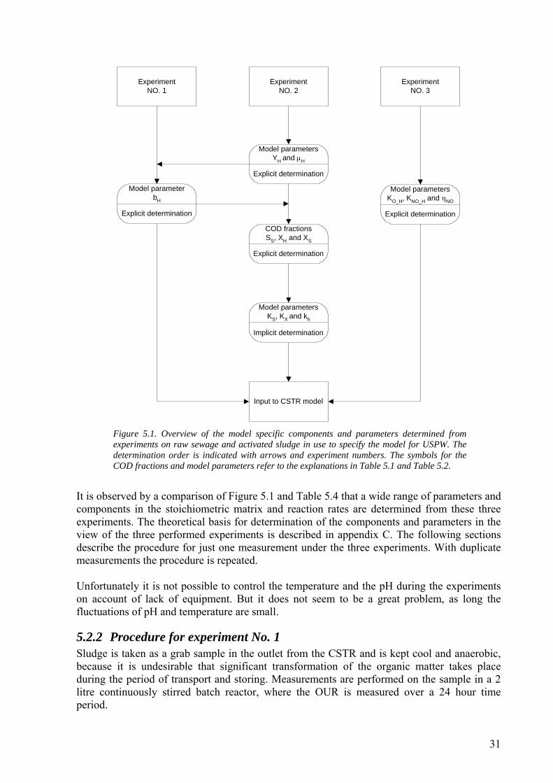
5.2.1 Performed experiments Two types of measurements are performed in order to determine the components and specific parameters for the model, oxygen uptake rate (OUR) and nitrate uptake rate (NUR). OUR and NUR-measurements are performed, because these analysis are the backbone for essential information about the condition of the sludge and provide input for the simulation purpose [Henze et al., 1995]. Both types of measurements are an investigation of the biomass’s influence on the relationship between the electron donor, organic substrate, and the electron acceptor, respectively dissolved oxygen and nitrate. It is assessed that performing the following approved experiments will give the most extensive investigation of the raw sewage and sludge.

• Experiment No. 1: Long term measurements of OUR on activated sludge in use • Experiment No. 2: Long term measurements of OUR with addition of readily

biodegradable substrate to raw sewage • Experiment No. 3: Short term measurements of OUR and NUR on activated

sludge in use Some of the information are derived by an explicit data interpretation, whereas other are determined by implicit fitting of data. Figure 5.1 shows the model specific components and parameters, which are determined and the approach for the determination order.

30

ExperimentNO. 1

Model parametersYH and µH

COD fractionsSS, XH and XS

Model parametersKS, KX and kh

Model parameterbH

ExperimentNO. 2

ExperimentNO. 3

Explicit determination

Explicit determination

Explicit determination

Implicit determination

Model parametersKO_H, KNO_H and ηNO

Explicit determination

Input to CSTR model

Figure 5.1. Overview of the model specific components and parameters determined from experiments on raw sewage and activated sludge in use to specify the model for USPW. The determination order is indicated with arrows and experiment numbers. The symbols for the COD fractions and model parameters refer to the explanations in Table 5.1 and Table 5.2.

It is observed by a comparison of Figure 5.1 and Table 5.4 that a wide range of parameters and components in the stoichiometric matrix and reaction rates are determined from these three experiments. The theoretical basis for determination of the components and parameters in the view of the three performed experiments is described in appendix C. The following sections describe the procedure for just one measurement under the three experiments. With duplicate measurements the procedure is repeated. Unfortunately it is not possible to control the temperature and the pH during the experiments on account of lack of equipment. But it does not seem to be a great problem, as long the fluctuations of pH and temperature are small.

5.2.2 Procedure for experiment No. 1 Sludge is taken as a grab sample in the outlet from the CSTR and is kept cool and anaerobic, because it is undesirable that significant transformation of the organic matter takes place during the period of transport and storing. Measurements are performed on the sample in a 2 litre continuously stirred batch reactor, where the OUR is measured over a 24 hour time period.

31

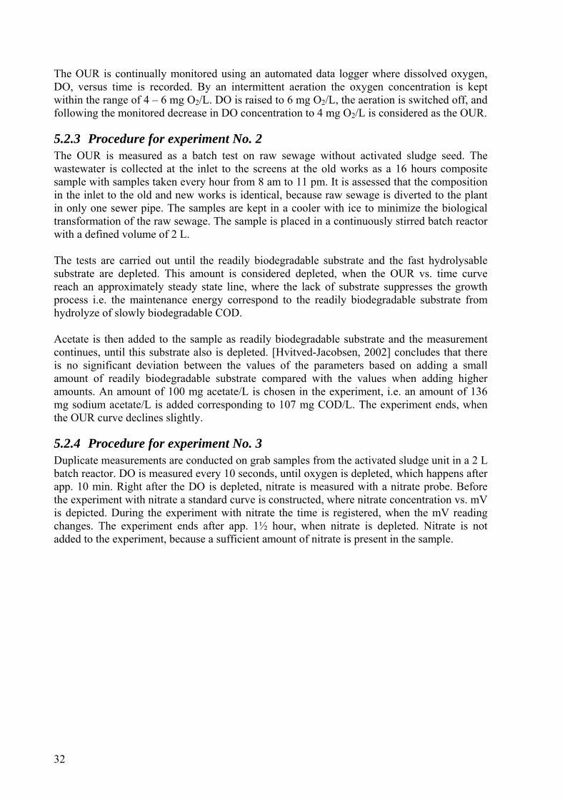
The OUR is continually monitored using an automated data logger where dissolved oxygen, DO, versus time is recorded. By an intermittent aeration the oxygen concentration is kept within the range of 4 – 6 mg O2/L. DO is raised to 6 mg O2/L, the aeration is switched off, and following the monitored decrease in DO concentration to 4 mg O2/L is considered as the OUR.

5.2.3 Procedure for experiment No. 2 The OUR is measured as a batch test on raw sewage without activated sludge seed. The wastewater is collected at the inlet to the screens at the old works as a 16 hours composite sample with samples taken every hour from 8 am to 11 pm. It is assessed that the composition in the inlet to the old and new works is identical, because raw sewage is diverted to the plant in only one sewer pipe. The samples are kept in a cooler with ice to minimize the biological transformation of the raw sewage. The sample is placed in a continuously stirred batch reactor with a defined volume of 2 L. The tests are carried out until the readily biodegradable substrate and the fast hydrolysable substrate are depleted. This amount is considered depleted, when the OUR vs. time curve reach an approximately steady state line, where the lack of substrate suppresses the growth process i.e. the maintenance energy correspond to the readily biodegradable substrate from hydrolyze of slowly biodegradable COD. Acetate is then added to the sample as readily biodegradable substrate and the measurement continues, until this substrate also is depleted. [Hvitved-Jacobsen, 2002] concludes that there is no significant deviation between the values of the parameters based on adding a small amount of readily biodegradable substrate compared with the values when adding higher amounts. An amount of 100 mg acetate/L is chosen in the experiment, i.e. an amount of 136 mg sodium acetate/L is added corresponding to 107 mg COD/L. The experiment ends, when the OUR curve declines slightly.

5.2.4 Procedure for experiment No. 3 Duplicate measurements are conducted on grab samples from the activated sludge unit in a 2 L batch reactor. DO is measured every 10 seconds, until oxygen is depleted, which happens after app. 10 min. Right after the DO is depleted, nitrate is measured with a nitrate probe. Before the experiment with nitrate a standard curve is constructed, where nitrate concentration vs. mV is depicted. During the experiment with nitrate the time is registered, when the mV reading changes. The experiment ends after app. 1½ hour, when nitrate is depleted. Nitrate is not added to the experiment, because a sufficient amount of nitrate is present in the sample.

32

6 Determination of COD fractions and parameters In order to make the model specific for the continuously stirred reactor at Umbilo Sewage Purification Works, COD fractions and parameters are determined in this chapter. The experiment numbers and procedures used to determine fractions and parameters are described back in section 5.2. This chapter is divided into a graphical presentation of the experimental results followed by a summary of the results, where the value of each COD fraction and parameters is compared to the default value from the ASM2 model. It is a foregone conclusion that the reader is familiar with appendix C, which lists the theoretical basis for determination of the fractions and parameters. CD-ROM annex 3 shows the calculation of the fractions and parameters for each individual experiment.

6.1 Graphical presentation of results

6.1.1 Experiment No. 1 Two oxygen uptake rate (OUR) measurements are conducted on two grab samples of activated sludge from the same day in October 2004. The experiment calculates the lysis and decay rate for the heterotrophic biomass, bH. Activated sludge is used, because the biomass is under substrate limiting conditions and the decrease in OUR over time reflect the lysis and decay rate. According to the theory the slope will be a straight line, when the natural logarithm of OUR is depicted against the time. [Henze et al., 1986] Figure 6.1 shows the natural logarithm of OUR vs. time for the two measurements.

y = -0,0333x + 2,3685R2 = 0,7061

y = -0,02x + 2,5069R2 = 0,42

0,0

1,0

2,0

3,0

4,0

0 5 10 15 20 25

Time [hr]

lnO

UR

Figure 6.1. OUR measurements on activated sludge where the natural logarithm of OUR vs. time is depicted.

The slopes of both measurements are almost straight lines as predicted from the theory, thus indicating successful experiments. The slope of each measurement is within a factor 1½ of each other seen as acceptable.

6.1.2 Experiment No. 2 OUR measurements on raw sewage with addition of readily biodegradable substrate are conducted to determine the COD fractions and parameters listed under experiment No. 2 in Figure 5.1. Raw sewage is used, because the COD fractions and parameters are associated with the characteristics of the inlet to the plant.

33

The COD fractions; SS, XS, XH, together with the stoichiometric parameter, YH, and the kinetic parameter, µH, are determined explicit, whereas the kinetic parameters, kh, KX, KS, are determined implicit. In the explicit determination the parameters and fractions are calculated from data interpretation of the equations for the OUR curve under different substrate conditions. The explicit determined values are incorporated into the equations and the implicit parameters are determined by fitting an OUR model to the actual measured OUR curve. The equations for the OUR curve are presented by the matrix model in table C.1 in appendix C. The concept of minimising the root mean square error (RMSE) is used to evaluate the fit. There are conducted 6 × 2 OUR measurements under experiment No. 2, however due to some difficulties with the equipment only 5 measurements (2 duplicates, 1 single) are considered to follow the theoretical OUR curve, see figure C.1 in appendix C, needed to calculate the fractions and parameters. The equipment difficulties ranged from power loss to an oxygen pump with insufficient capacity to keep the solution of raw sewage aerated between 4 – 6 mg O2/L. The samples are collected from October to December 2004. Figure 6.2 a) and b) plus c) and d) show the duplicates, whereas e) shows the single measurement. Figure 6.2 f) gives an example of one of the experiment, where the magnetic stirred has failed, hence the characteristics peak for readily biodegradable substrate in the beginning of the curve pattern is not present. The measured OUR curve is modelled until the addition of readily biodegradable substrate, in order to any eventually uncertainties related to the addition from the model.

34

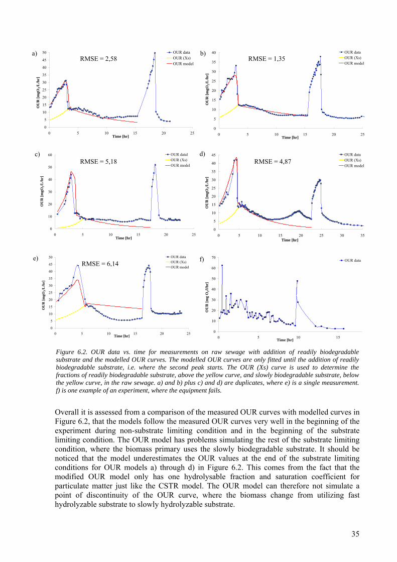
0

5

10

15

20

25

30

35

40

45

50

0 5 10 15 20 25Time [hr]

OU

R [m

gO2/L

/hr]

OUR dataOUR (Xs)OUR model

0

5

10

15

20

25

30

35

40

0 5 10 15 20 25Time [hr]

OU

R [m

gO2/L

/hr]

OUR dataOUR (Xs)OUR model

a) b)

c) d)

e) f)

0

10

20

30

40

50

60

0 5 10 15 20 25Time [hr]

OU

R [m

gO2/L

/hr]

OUR datalOUR (Xs)OUR model

0

5

10

15

20

25

30

35

40

45

0 5 10 15 20 25 30 35Time [hr]

OU

R [m

gO2/L

/hr]

OUR dataOUR (Xs)OUR model

0

5

10

15

20

25

30

35

40

45

50

0 5 10 15 20 25Time [hr]

OU

R [m

gO2/L

/hr]

OUR dataOUR (Xs)OUR model

0

10

20

30

40

50

60

70

0 5 10 15Time [hr]

OU

R [m

g O

2/l/h

r]

OUR data

RMSE = 5,18

RMSE = 2,58 RMSE = 1,35

RMSE = 4,87

RMSE = 6,14

Figure 6.2. OUR data vs. time for measurements on raw sewage with addition of readily biodegradable substrate and the modelled OUR curves. The modelled OUR curves are only fitted until the addition of readily biodegradable substrate, i.e. where the second peak starts. The OUR (Xs) curve is used to determine the fractions of readily biodegradable substrate, above the yellow curve, and slowly biodegradable substrate, below the yellow curve, in the raw sewage. a) and b) plus c) and d) are duplicates, where e) is a single measurement. f) is one example of an experiment, where the equipment fails.

Overall it is assessed from a comparison of the measured OUR curves with modelled curves in Figure 6.2, that the models follow the measured OUR curves very well in the beginning of the experiment during non-substrate limiting condition and in the beginning of the substrate limiting condition. The OUR model has problems simulating the rest of the substrate limiting condition, where the biomass primary uses the slowly biodegradable substrate. It should be noticed that the model underestimates the OUR values at the end of the substrate limiting conditions for OUR models a) through d) in Figure 6.2. This comes from the fact that the modified OUR model only has one hydrolysable fraction and saturation coefficient for particulate matter just like the CSTR model. The OUR model can therefore not simulate a point of discontinuity of the OUR curve, where the biomass change from utilizing fast hydrolyzable substrate to slowly hydrolyzable substrate.

35

The problem solver in Excel is used to implicit determine the model constants with default values as the initial values. The default values for KS, KX and kh are respectively 8 g COD/L, 0,1 g COD/g COD, 3 g COD/(g COD ⋅ d) [Henze et al., 1995]. The solver is limited to realistic solutions as the values of KS, KX and kh are restricted with upper bounds of initial value × 50 and lower bounds of initial value × 1

50 , hence unrealistic values are excluded.

6.1.3 Experiment No. 3 OUR and nitrate uptake rate (NUR) measurements are conducted on activated sludge to determine the saturation coefficient for oxygen, KO_H, and nitrate, KNO_H, for heterotrophic biomass based on the monod equation and the reduction factor for denitrification, ηNO, from the relation between NUR and OUR. Activated sludge is used, because the amount of readily biodegradable substrate is consumed and will not interferer with the measurements. The oxygen and nitrate respiration results will then only be a function of the concentrations of dissolved oxygen (DO) and nitrate. [Kappeler and Gujer, 1992] There are conducted duplicate measurements on two samples of activated sludge collected in December 2004. However in Figure 6.3 and Figure 6.4 are only the measurements from one sample depictured, as the measurements from the other sample are similar. The saturation coefficients can be determined either by a regular plot of uptake rate vs. concentration or a plot of inverse uptake rate vs. inverse concentration. The saturation coefficient for oxygen is determined by the inverse plot, whereas the regular plot is used to determine the coefficient for nitrate. In Figure 6.3 is the inverse plot of OUR vs. DO concentration shown.

y = 43x + 205

y = 22x + 96

0

50

100

150

200

250

300

350

0,0 0,5 1,0 1,5 2,0 2,5 3,0 3,5 4,0

1/(DO) [L/mg O2]

1/(O

UR

) [se

c L

/mg

O2]

Figure 6.3. Inverse plot of OUR vs. DO concentration of duplicate measurements on activated sludge.

The measurements in Figure 6.3 follow straight lines like the theory states, however there is some fluctuations in the range of high DO concentrations. The saturation coefficient of oxygen for the heterotrophic biomass, KO_H, can be determined as b

O _ H aK = , where y = a · x + b. In Figure 6.4 is the plot of NUR vs. nitrate concentration shown, where a) shows the plot of the first measurement and b) shows the subsequent measurement, where the sample has been aerated in between to convert ammonium to nitrate.

36

a) b)

0,0

1,0

2,0

3,0

4,0

5,0

6,0

0,0 2,0 4,0 6,0 8,0 10,0 12,0 14,0 16,0NO3 [mg N/L]

NU

R [ µ

g N

/L/s

ec]

NURmax

½ NURmax

Figure 6.4. The NUR vs. the nitrate concentration. The saturation coefficient of nitrate can be determined at half of NURMAX.

0,0

0,5

1,0

1,5

2,0

2,5

3,0

3,5

4,0

4,5

0,0 5,0 10,0 15,0 20,0

NO3 [mg N/L]

NU

R [ µ

g N

/L/s

ec]

NURmax

½ NURmax

The measurement starts at high nitrate concentrations and as the microorganisms utilize nitrate the concentration drops. The lower measured NUR values compared to NURmax at high nitrate concentrations in Figure 6.4 a) results from the fact, that the microorganisms are not adapted to nitrate as electron acceptor and require a phase to switch from oxygen to nitrate as electron acceptor. In Figure 6.4 b) the microorganisms are getting used to nitrate as electron acceptor and the NUR values are at high nitrate concentration closer to NURmax than in the first measurement. The saturation coefficient for nitrate, KNO_H, is determined as the nitrate concentration at ½ ⋅ NURmax. Figure 6.5 depictures respectively the concentration of DO vs. time and the concentration of nitrate vs. time. The slope in a) is OUR and in b) NUR. The reduction factor for denitrification, ηNO, is calculated as the slope of NUR divided with the slope of OUR. Note that the units in the calculation must be electron equivalents per litre per second.

y = -0,0014x + 10,39R2 = 0,9984

y = -0,0014x + 10,872R2 = 0,9996

0,0

2,0

4,0

6,0

8,0

10,0

12,0

0 1000 2000 3000 4000 5000 6000Time [sec]

NO

3 [m

g N

/L]

Test 1Test 2

y = -0,0046x + 7,86716,0

7,0

8,0

9,0

/L]

Test 1Test 2

y = -0,0058x + 6,6207R2 = 0,9864

R2 = 0,9991

0,0

1,0

2,0

3,0

4,0

5,0

0 200 400 600 800 1000 1200 1400 1600 1800 2000

Time [sec]

DO

[mg

O2

Figure 6.5. a) The concentration of DO vs. time and b) the concentration of nitrate vs. time. The slope is respectively the OUR and NUR.

a) b)

Figure 6.4 and Figure 6.5 b) are peculiar in the sense, that the nitrate concentration never reaches zero. This can be caused by interference from compounds in the wastewater, which affect the mV reading. Interference from bicarbonate, chloride, ortho-phosphate and fluoride are investigated, but the concentrations in the raw sewage are not high enough to cause a significant interference, see annex VI. There are however 11 other compounds, which can

37

interfere with the nitrate reading, but the compounds are not measured in the raw sewage, thus they cannot be excluded as explanation.

6.2 Summary of results A set of 3 COD fractions and 9 model parameters is determined accordingly to Figure 5.1 as a basis for model specific input. Table 6.1 summarizes the results from the experiments on activated sludge and raw sewage. The total set of determined COD fractions and model parameters are listed in CD-ROM annex 4.

Table 6.1. Summary of results from COD fractions and model parameters compared with default values at 20°C given in [Henze et al., 1995]. The COD fractions are determined on raw sewage with a mean total COD value on 775 mg COD/L. The ASM2 values are corrected for this.

Specific model input Symbol Unit Mean Std. dev. ASM2 No. 1

Readily biodegradable substrate 2 SS mg COD/L 145 50 150 2 5

Slowly biodegradable substrate 3 XS mg COD/L 580 235 540 3 5

CO

D

Frac

tions

Heterotrophic biomass XH mg COD/L 50 30 90 5

Yield coefficient YHg COD

g COD 0,53 0,06 0,63 5

Lysis and decay rate bH d-1 1,2 0,4 0,4 2

Maximum growth rate µH d-1 7,3 3,4 6 5

Saturation coeff. for SS KS mg COD/L 8,2 6,4 4 /4 4 5

Hydrolysis rate constant kh ( )g COD

g COD d⋅ 4,2 3,0 3 5

Saturation coeff. for particulate COD KXg COD

g COD 0,89 1,03 0,10 5

Saturation coeff. for oxygen KO_H mg O2/L 0,29 0,10 0,20 4

Saturation coeff. for nitrate KNO_H mg N/L 4,9 0,9 0,5 4

Mod

el

Para

met

ers

Reduction factor for denitrification ηNO - 0,14 0,03 0,8 4 1: Number of measurements used to determine the specific model input. 2: The readily biodegradable substrate includes fast biodegradable substrate and fermentation products, SS =S + SF A. 3: The slowly biodegradable substrate in the OUR model includes inert soluble and particulate matter, X = X + XS, OUR S, ASM2 I + SI. 4: Saturation coefficients for respectively fast biodegradable substrate and growth on fermentation products. These values correspond to a KS = 8.

A comparison between the average experiments results for model parameters and the default values from ASM2-model reveals the following differences, i.e. the CSTR model is compared to the ASM2 model;

• Since the measured YH is slightly lower, the heterotrophic biomass in the CSTR is not as efficient at utilizing the substrate in the wastewater as a typical biomass. This means in the CSTR model that the biomass grows less on the same amount of readily biodegradable substrate compared to typical biomass.

• The higher bH results in a lower concentration of active heterotrophic biomass in the CSTR and a larger risk of the biomass getting washed out of the CSTR, if the sludge retention time is lowered. The higher µH gives just the opposite effect.

• The determined value for KS is similar to the ASM2 value.

38

• The higher kh increases the hydrolysis rate, whereas the higher KX lowers it. The XS

XHXS

X XHK +

, overall difference depends on the monod equation for particulate COD,

and the value of kh. • The determined value for KO_H is similar to the ASM2 value. • The higher KNO_H and the lower ηNO both decrease the denitrification rate.

When the peculiar results from the graphical presentation of KNO_H and ηNO are related to the

latively large deviation from the ASM2 values in Table 6.1, it is assessed that these arameters sensitivity for the model results should be investigated, if the CSTR model is capable of modelling the denitrification process.

repin

39

7 WEST-Model WEST (Worldwide Engine for Simulation, Training and automation) is a software program designed for simulation of environmental systems, such as wastewater treatment plants, rivers and catchment areas. The program is used at universities in 13 different countries, including University of Kwazulu-Natal in South Africa, as an integrated tool for simulation and automation of environmental systems and a general training in how these systems operate. [www.hemmis.com, 2004] In this and the following chapter the WEST program is used to simulate the COD and ammonium removal at the new works at Umbilo Sewage Purification Works and to propose options for optimization. The activated sludge model in section 5.1 for modelling aerobic utilization of substrate, nitrification and denitrification in the continuously stirred reactor is in this chapter incorporated as an single unit, when the new works is implemented in WEST.

7.1 Introduction to the WEST program WEST consists of a graphical user interface with a highly hierarchical program structure in which subprograms can be accessed. All the subprograms are defined by a collection of text files in the model library. The WEST program is managed by MSL (Model Specification Language), a language used to represent and specify the subprograms in the model library. WEST consists of 4 different subprograms with a graphical user template, where the user accesses the different utilities in the programs. The four subprograms are:

• WEST manager • WEST configuration builder • WEST experimental environment • WEST model editor

[www.hemmis.com, 2004] On the grounds of the hierarchical structure it is possible to access all the utilities in WEST from the four subprograms.

7.1.1 Subprograms The WEST manager gives the user an overview of the different project created and allows for new projects to be created. With each created project is a list of the different configuration and/or experiments assigned to that project. [WEST tutorial, 2004] In the WEST configuration builder the user selects the desired activated sludge model among default models already implemented in the WEST hierarchical structure or design an alternative model. The selected model is the foundation for the biological and chemical components used as input variables to the specific wastewater treatment plant. The wastewater treatment plant is then represented by the different treatment processes and connections between them. The treatment processes are represented by different units, such as primary clarifier, activated sludge unit, secondary settler, etc., where each unit has its own sub-model. [WEST tutorial, 2004] The WEST experiment environment is based on the activated sludge model and the sub-models selected in the WEST configuration builder. In the WEST experiment environment the user sets the values of the variables and parameters specific to each sub-model. The user has an option

40

of running different types of scenarios, which can be used to calibrate and optimize the implemented model of the plant. [WEST tutorial, 2004] In the WEST model editor the user can design an alternative model by use of the matrix notation and implementing it in the WEST hierarchical structure. The WEST model editor is also used to program the different text files, which control the WEST hierarchical structure, in MSL. [WEST MSL reference guide, 2004]

7.1.2 WEST solution procedure The sub-models presented in the WEST configuration builder are all expressed in terms of fluxes. In processes dealing with liquids and suspension, concentrations are usually measured in the liquid phase. When a concentration is given in g per m3, the volume indication m3 stands for the amount of water or suspension and not for the total volume, including the gas phase. Using fluxes the conservation of mass is expressed as follows:

( )( )

d M0

d t=

[WEST models guide, 2004] where M= mass in the entire system for each component The mass M can be broken down into the different components Mi; water, biological and chemical components. The mass balance in a tank with a certain volume and different incoming and outgoing flows α can be written as following ordinary differential equations:

( )( ) ( )

( )( )

ii i

ii i α

d Mr V

d t

d V 1d t

αα

α

= φ + ⋅

⎛ ⎞= ⋅ φ⎜ ⎟ρ ⎠

∑

∑ ∑

[WEST models guide, 2004]

i 3

logy stated above, i.e. the equations can be seen as the controlling quations t

differential qsimultaneouslynumericall n

-

⎝

where: = mass of component [g] M

V = volume of the tank [m ] φiα = net in/out flux of component i in the flow α [g/s] ri = reaction speed of component i [g/m3/s] ρi = density of component i [g/m3] Based on the sub-model selected for each unit WEST sets up algebraic equations for the entire

lant using the methodope of he system. When WEST performs a simulation, the system of ordinary

e uations are numerically integrated in time and the algebraic equations are solved. The user can select three methods by which WEST performs the ty i egration:

Fixed step size integrator. A fixed step size integrator is an integrator that takes a constant time step in order to solve the integration of the system of ordinary differential equations.

41

-

- Stiff solver. A stiff solver obtains a high performance gaSystems of equations that have vastly different time constants are called stiff.

cally, perhaps by orders of magnitude. [WEST help, 2005]

m the new works, it is assessed, that the mechanical eatment does not have significant impact on the COD and ammonium removal as the

arger particles and grains of sand. The anaerobic igesters only have an effect on the sludge condition, thus limited impact on the COD

ST licence restrictions.

Adaptive step size integrator. An adaptive step size integrator is an integrator that modifies its time step size in order to obtain optimal calculation speed and optimal calculation accuracy.

in for stiff systems.

They are stiff in the sense, that the equations with the longer time constants will not change hardly at all, i.e. stiff, in the time it takes the other, less stiff, equations to change drasti

The integrator in the following WEST model is an adaptive step size (Runge-Kutta of 4th order adaptive step size controller) chosen for its speed and accuracy. The step size during simulation ranges from 5·10-4 to 1 day.

7.2 Implementation of the new works in the WEST program The new works at Umbilo Sewage Purification Works is implemented in the WEST program on the basis of the layout described in section 3.3.2. It is however not possible to implement the entire layout due to restrictions in the WEST licence purchased by the University of Kwazulu – Natal. The University does not have license for the mechanical treatment process nor the anaerobic digester unit and no sub-models are therefore available for the two units in the WEST configuration builder. Given that the implemented model is used to optimize COD and ammonium removal in the effluent frotrprimary purpose of the mechanical treatment process is to protect the driving parts of the pumps used in other treatment process from ldfractions and ammonium in the effluent.

Figure 7.1 shows the new works implemented in the WEST configuration builder as a composition of the different treatment units.

Figure 7.1. The model of the new works in the WEST program. The mechanical treatment process and the anaerobic digesters are not modelled due to WE

42

7.2.1 Selection of sub-models In the following are each unit discussed and the sub-model selecte . d In appendix D are the other available sub-models described.

Inlet: Influent of raw sewage and supernatant from belt press The Influent unit allows the user to enter the volumes and composition of the raw sewage, either as constant values used in a steady-state simulation or as changing values used for a dynamic simulation. The flow and concentrations of the supernatant from the belt press are implemented in the model as a unit, which generates constant flow and concentrations. A

is cho a sition and flow of the constant generator unit sen, because it is assessed th t the composupernatant does not change significantly due to the long sludge retention time in the anaerobic digesters, hence fluctuations are equalized.

Concentration to Flux and Flux to Concentration converters Since fluxes enter into the ordinary differential equations and the input file in the Influent unit is given in concentrations, a conversion is needed. The Concentration to Flux (C/F) unit is used to convert incoming data expressed in concentrations into fluxes as a product of

flow. ust the opposite happens in the Flux to Concentration (F/C) unit, concentration and Jwhere the fluxes are converted to concentrations.

Primary clarifiers WEST gives the user a choice of six different sub-models for simulating primary clarifiers listed in appendix D. The primary clarifiers are chosen to be point settlers, which is the simplest sub-model. The modelling of a primary clarifier by means of a point settler is a simplification of the actual process. The point settler is only a phase separator, and has no real volume. Hence, the sub-model does not take into account the retention time in the settler. It is not a dynamical sub-model but only based on mass balances. The two primary clarifiers are

nly represented as one point settler because the same mass balance is achieved, wo hen the

oint ettler are shown in Table 7.1. The underflow rate, Uunder, is calculated by a mass balance over

the primary c -settable suspended solids, fns, is calibrated against COD m

le 7.1. Th sub- l.

Symbol Description Value Unit

underflow is doubled. The particulate concentration in the effluent is calculated as a fraction of the influent concentration to the settler. To calculate the underflow concentration a mass balance over the settler is solved. It is assumed that there are no biological reactions. The other sub-models might be better to describe the actual condition assumed that all parameters are known in the primary clarifiers due to their greater complexity. The sub-models include 4 to 10 parameters but with the limited dataset available for the clarifiers is it only possible to determine a minority of these. For the point settler 2 out of 2 parameters can be estimated, which makes it the preferred solution. The two specific parameters for the ps

larifiers as shown in Figure 3.8, whereas the fraction of noneasurements from the primary clarifiers’s effluent.

Tab e two specific parameters for the point settler mode

Q The underflow rate 130 [m3/d] underfns Fraction of non-settable suspended solids 0,5 [-]

43

Two and three combiners The combiner units are simple addition units, where the fluxes of either a component or water into the unit are combined. There are 2 different types of combiners; a two combiner, which combines two fluxes and a three combiner, which combines three fluxes. The outflow combiner unit is a three combiner whereas the other 4 in Figure 7.1 are two combiners.

CSTR There are four different sub-models available for the activated sludge unit listed in appendix D. The choice lies between a unit where the effluent flow rate is controlled by a pump, a unit where the volume can vary, one fixed volume tank or several fixed volume tanks in series where the influent flow is equal to the effluent flow. A pump does not control the effluent from the CSTR at the new works and the CSTR consists only of one tank also. The influent to the CSTR is assumed fairly constant and does not cause a change in the water level in the tank. The fixed volume tank will therefore be used as sub-model for the CSTR. The influent is

ed constant, because USPW only receives sewage water for domestic and industrial assumorigin and does not receive any rainwater, which can cause large fluctuations in the inlet flow. The flow data in section 4.1.1 also shows relative constant flow into the new works. The two primary clarifiers will also act as buffer tanks and equalize the fluctuations in the flow to the CSTR. The sub-model includes 27 parameters, which are listed in annex VII.

Two and three splitters There are two different types of splitters; a two splitter with two outlets and a three splitter with three outlets. There are also two sub-models available for the two types of splitters, an absolute splitter, where the underflow is a constant value and a relative splitter, where the underflow is a fraction of the inlet. The splitters implemented at the secondary settler and dissolved air flotation (D.A.F.) station are both two splitters. The splitter at the secondary

, which means the two secondary settlers are settler is a relative splitter with a fraction of 0 5,loaded identically. The splitter at the D.A.F. station is an absolute splitter with a constant value of 690 m3/d as influent to the D.A.F. station. The splitter is an absolute splitter, because the station is feed by gravity flow, which is assessed to be full flowing all the time and thereby fairly constant.

Secondary settlers and D.A.F. station There are six different sub-models available for the secondary settlers listed in appendix D. It is assessed that the point settler sub-model, which was used to describe the primary clarifier, cannot describe the actual conditions in the secondary settler adequately. When a secondary settler is designed two very important design parameters are the surface area and height of the tank [Ekama et al., 1997] and it is assessed that the sub-model has to include these two parameters in order to model the actual conditions in the secondary settler with acceptable ccuracy. On the basis of this assessment the Takacs sub-model is chosen. The sub-model

al flow is considered.

4 out of 9 parameters for the model are estimated and default values are used for the remaining parameters. The estimated and default parameter values are listed in Table 7.2. The threshold

adivides the settlers in a number of horizontal layers, which make them capable of modelling the true settling behaviour of the secondary settlers and the vital functions; clarification and thickening. Solids mass balances are calculated around the layers, where two assumptions are in force; the incoming solids are distributed immediately homogenous over the feed layer and only vertic

44

con is est annex 1.

e The estimated an ult mete del used to model the two nd settlers.

Parameter

centration of suspended solids, XT, represents the highest concentration in the layers and imated as the minimum sludge volume index in the activated sludge unit, see CD-ROM

Tablseco

7.2. d defa para r values for the Takacs sub-moary

Value Unit Description H 2,9 m Height of the clarifier A 800 m2 Surface area of the clarifier XT 40.000 g/m3 Threshold suspended solids concentration

r 5 er COD

Estim

ated

Qunde

F_TS.000 m3/d The underflow from the secondary settl

S_ 0,75 - Fraction TSS/COD r_H 0,0 6 r_P 0,00286 m3/g Settling parameter (low concentration)

m practical settling velocity

alu

X_Lim 900 g/m3 Minimal concentration in sludge blanket

0057 m3/g Settling parameter (hindered settling) es

v0 474 m/d Maximum theoretical settling velocity v00 250 m/d MaximuD

efau

lt v

The Table 7.3 shows the estimated param

le 7.3. The e ted rame used to model the D.A.F. n. Default e for

eter V

D.A.F. station is modelled similar to the secondary settlers with the Takacs sub-model. eter values.

Tabtio

s atim pa ter values for the Takacs sub-modelsta values ar used the remaining 5 parameters, see Table 7.2.

Param alue Unit Description H 2,9 m Height of the D.A.F. station A 05 m2 Surface area of the D.A.F. station

3XT 40.000 g/m Threshold suspended solids concentration Qunder 100 m3/d The underflow from the D.A.F. station

Loop breaker There are 2 sub-models available for the loop breaker unit, loop breaker and differential loop

reaker. Both sub-models are used to accelerate the simulation performance, especially when tment plant. The loop breaker

bcycles are present in the configuration of the wastewater treaintroduces a time delay represent g the retenin tion time in the loop. The differential loop breaker is selected with an exponential time delay of 0,0005 d-1.

Outlet: effluent of treated sewage and sludge The effluent unit for treated sewage gives the user the options to have the results of the selected components graphically depicted or written to a text file. The user selects the

e data being stored or components by checking them off in the other units, i.e. it is possible to follow the development of components after every single unit. The frequency of thdepicted is also set in the effluent unit. Both effluent unit and waste unit are boundary conditions, where the WEST model can discharge the treated effluent and sludge.

7.3 Calibration of the model in the WEST program In order to get a model that can simulate the actual conditions at the works and reproduce real data the model is calibrated. With the object of simplifying the calibration procedure of the WEST model and limiting the numbers of parameters, only calibration of the parameters in the

45

CSTR model described in section 5.1 with regards to the COD removal, nitrification and denitrification is performed. It is assessed that these processes are calibrated when respectively measured concentrations of total COD, ammonium, nitrate and organic nitrogen (the variables) in effluent not deviate significantly from the simulated values. WEST is capable of calibrating

e selected parameters automatically, but the authors have not been able to increase the step size du g acceptable long time. T divided int

• ent of model results without any calibration initiative. • A preliminary investigation, where it is assessed what type of calibration, static or

et in section 6.2 is sufficient to calibrate the easured variables in the effluent. The assessment consists of a comparison of the measured

median concentra ith steady state simulated values of COD and nitrogen, where the experimentally determined and default parameters are inc put, Table 7.

o of red and steady te sim d the t th ork 003.

thrin the calibration, which means a step size of 1 · 10-6 d-1 takes unhe authors have opted to calibrate the CSTR model manually, where the calibration is

o 3 parts:

An assessm

dynamic, is possible with the available dataset. • A calibration where the parameters are calibrated on measurements of the four

variables.

7.3.1 Assessment of model results without calibration The results from the model without any further calibration initiative are used to assess, if the previously experimentally determined datasm

tions of COD and nitrogen in the effluent from 2003 w

luded as in 4.

Table 7.4. Cvalues from

mparison effluent a

measue new w

sta ulates in 2

Variable COD NH4 NO3 Org-N Measured [mg/L] 89 4,3 4,0 2,6 Simulated [mg/L] 89,5 0,7 26 1,0

The model is under steady state conditions able to simulate the COD removal satisfactory. This is also expected, since most of the parameters, which affect the COD removal, are experimentally determined. The model is however not able to simulate the nitrogen fractions, especially nitrate differs significantly. An explanation of this could rely in the determination of

o of the parameters, the reduction factor for denitrification, ηNO, and the saturation

ed and measured in Table

e and COD with daily measurements as input. The available dataset only ontains app. 4 measurements of Total Kjeldahl Nitrogen, TKN, every month and since

twcoefficient for nitrate, KNO, in accordance with section 6.2, where it is stated that the values differs considerably from ASM2 values. The importance of the two parameters on the nitrogen concentrations is therefore investigated further in the subsequent sections.

The large difference between the concentrations of nitrate simulat7.4 could originate from the possibility that the model cannot simulate denitrification accurately before a more intensively calibration procedure is performed.

7.3.2 Preliminary investigation of the available data set The preliminary investigation assesses the possible calibration types, which can be performed based on the available data set from 2003. The static calibration requires average measurements of the variable, whereas the dynamic calibration requires continuously measurements. Based on the available data set, the dynamic calibration is only performed on ammonium, nitratc

46

organic nitrogen is measured as TKN subtracted the concentration of ammonium it is assessed, that the frequency of measurements only allows the performance of a static calibration on rganic nitrogen.

le is sed for the dynamic calibration. Both input files include the flow rate of the raw sewage into

re measured daily with a w exceptions, where linear interpolation is performed to estimate the missing values. The

re therefore set to zero. The concentration of atmospheric nitrogen in wage water is set to the default values from the ASM2 model at 20 °C. The concentration of

and set to zero. In Table 7.5 are the COD fractions for the steady state input file shown and the dynamic input file

atios multiplied by the daily total COD

beginning of any simulation, otherwise the WEST model uses part of the simulation period to

Tabl .5. The COD ons in the steady state input file. The unit is mg 2/L

Fraction Concentration 1

o Both calibrations needs input files, where the measurements of the variables are listed either as average or daily measurements. Steady state and dynamic input files The steady state input file is used for the static calibration, whereas the dynamic input fiuthe new works and the concentrations of the 11 variables used in the CSTR model, see Table 5.4. There are measurements of flow rate, ammonium, alkalinity and total COD, whereas the concentrations of oxygen, nitrate, atmospheric nitrogen and COD fractions are estimated. The flow rate is measured daily without exceptions. The steady state input file uses the mean value, which is 8.000 m3/d, whereas the dynamic input file uses the actual daily measurements. The ammonium, alkalinity and COD concentrations afesteady state input file uses the mean value for ammonium and alkalinity based on the daily measurements, which are respectively 25 mg N/L and 2 mole HCO3

-/L. The COD fractions are estimated from an average total COD concentration of 640 mg O2/L. The estimated values for the concentrations of oxygen, nitrate and atmospheric nitrogen are identically in both files. It is assumed that the conditions in the sewer system are anaerobic, as the oxygen transfer from the air in the sewer pipes to the sewage is negligible. With no oxygen available in the sewage, nitrate cannot be produced in the nitrification process and it is assumed that the available concentration of nitrate is utilized quickly. The concentrations of oxygen and nitrate asefree nitrogen in the influent is of no importance to the CSTRproduced in the denitrification process in the matrix and is nconversion factors. The fractions of COD are calculated from an estimated and experimentally determined composition of total COD. X

model, because it is only ot part of any equations or

e 7 fracti

O

SS 120 SIX

74 I 62

I is estimated from the ASM2 model. SI is estimated as 90% of the soluble COD concentration in the effluent [Henze et al., 1995], whereas SS, XS and XH are based on the experiments. Under the assumed anaerobic condition autotrophic biomass, XAUT, cannot grow and the concentration in the influent is assumed negligible

is based on the same rmeasurements. The dynamic input file is shown in CD-ROM annex 5.

7.3.3 Calibration Before the calibration can be performed, the WEST model needs to reach an equilibrium, i.e. a situation where the variables are constant. It is important that the model is at equilibrium in the

XS 343 XH 41

X 0 AUT1: Based on 640 mg COD/L

47

stabilize the variables in each sub-model. The equilibrium can be reached by running a steady state simulation over a longer period with constant influent flow and concentrations. The

eriod used is a 100-day period with the steady state input file. The values of variables in the

hanging the nitrogen content in the COD fractions, iN, performs the static calibration on the

ameters selected and these parameters are calibrated ith a dynamic calibration. The parameter values in the dynamic calibration are accepted on

es of ammonium, itrate and COD effluent concentrations.

The WE

procedure for the WEST model. The steady state run achieves equilibrium for performing

Steady Staterun

psingle sub-models at the end of the steady state simulation are used as initial values for the variables in the subsequent calibrations. Ccontent of organic nitrogen. The parameters are saved and subsequently used in the sensitivity analysis and dynamic calibration. A sensitivity analysis is used to identify the parameters affecting the effluent concentrations of ammonium, nitrate and COD, i.e. parameters not previously determined plus ηNO and KNO. On the basis of the sensitivity analysis are parwthe basis of the lowest RMSE value between measured and simulated valun

ST model is calibrated by using the procedure shown in Figure 7.2.

The end value ofthe variables aresaved as initial

values

Use steady stateinput file

Enter initial valuesfor variables in the

sub-models

A steady statesimulation is runover 100 days

Use dynamic inputfile

Use steady stateinput file

Staticcalibration

Variable organic N

Calibrate iN

Save the value ofiN

Dynamiccalibration

Calibrate sensitiveparameters

Use dynamic inputfile

The WEST modelis calibrated

Sensitivityanalysis

VariablesCOD, SNO, SNH

Not experimentaldetermined

parameters +ηNO and KNO

VariablesCOD, SNO, SNH

RMSEcontrol

Save the value ofthe parameters

Figure 7.2. Calibrationof a static calibration thereafter a sensitivity analysis and at last a dynamic calibration on the sensitive parameters.

48

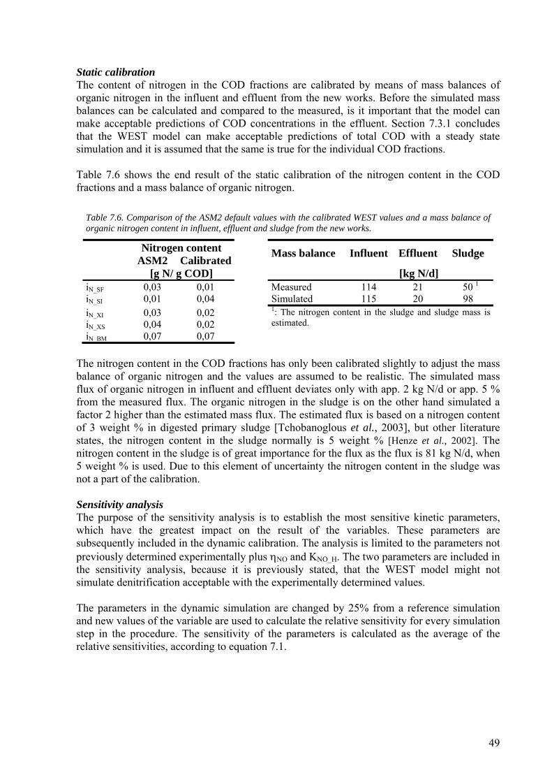
Static calibration The content of nitrogen in the COD fractions are calibrated by means of mass balances of organic nitrogen in the influent and effluent from the new works. Before the simulated mass balances can be calculated and compared to the measured, is it important that the model can

ake acceptable predictions of COD concentrations in the effluent. Section 7.3.1 concludes

or the individual COD fractions.

T fr

able 7.6. Co f t valu ed ue s rganic nitro nd udge from the new works.

gen co

mthat the WEST model can make acceptable predictions of total COD with a steady state simulation and it is assumed that the same is true f

able 7.6 shows the end result of the static calibration of the nitrogen content in the CODactions and a mass balance of organic nitrogen.

T mparisongen

of the ASM2 det, effl

aul es with the calibrat WEST val s and a mas balance ofo content in influen uent a sl

Nitro ntent A Calibrated

nce Influent Effluent Sludge

/ g CO114 21 50 1

SM2 Mass bala

[g N D] [kg N/d] Measured iN_SF 0,03 0,01

iN_SI 0,01 0,04 Simulated 115 20 98 i 0,03 0,02 N_XIiN_XS 0,04 0,02 estimated. i

1: The nitrogen content in the sludge and sludge mass is

N_BM 0,07 0,07 The nitrogen content in the COD fractions has only been calibrated slightly to adjust the mass balance of organic nitrogen and the values are assumed to be realistic. The simulated mass flux of organic nitrogen in influent and effluent deviates only with app. 2 kg N/d or app. 5 % from the measured flux. The organic nitrogen in the sludge is on the other hand simulated a factor 2 higher than the estimated mass flux. The estimated flux is based on a nitrogen content of 3 weight % in digested primary sludge [Tchobanoglous et al., 2003], but other literature states, the nitrogen content in the sludge normally is 5 weight % [Henze et al., 2002]. The

itrogen content in the sludge is of great importance for the flux as the flux is 81 kg N/d, when ue to this element of uncertainty the nitrogen content in the sludge was

parameters not reviously determined experimentally plus ηNO and KNO_H. The two parameters are included in

a reference simulation nd new values of the variable are used to calculate the relative sensitivity for every simulation

in the procedure. The sensitivity of the parameters is calculated as the average of the relative sensitivities, according to equation 7.

n5 weight % is used. Dnot a part of the calibration. Sensitivity analysis The purpose of the sensitivity analysis is to establish the most sensitive kinetic parameters, which have the greatest impact on the result of the variables. These parameters are subsequently included in the dynamic calibration. The analysis is limited to the pthe sensitivity analysis, because it is previously stated, that the WEST model might not simulate denitrification acceptable with the experimentally determined values. The parameters in the dynamic simulation are changed by 25% fromastep

1.

49

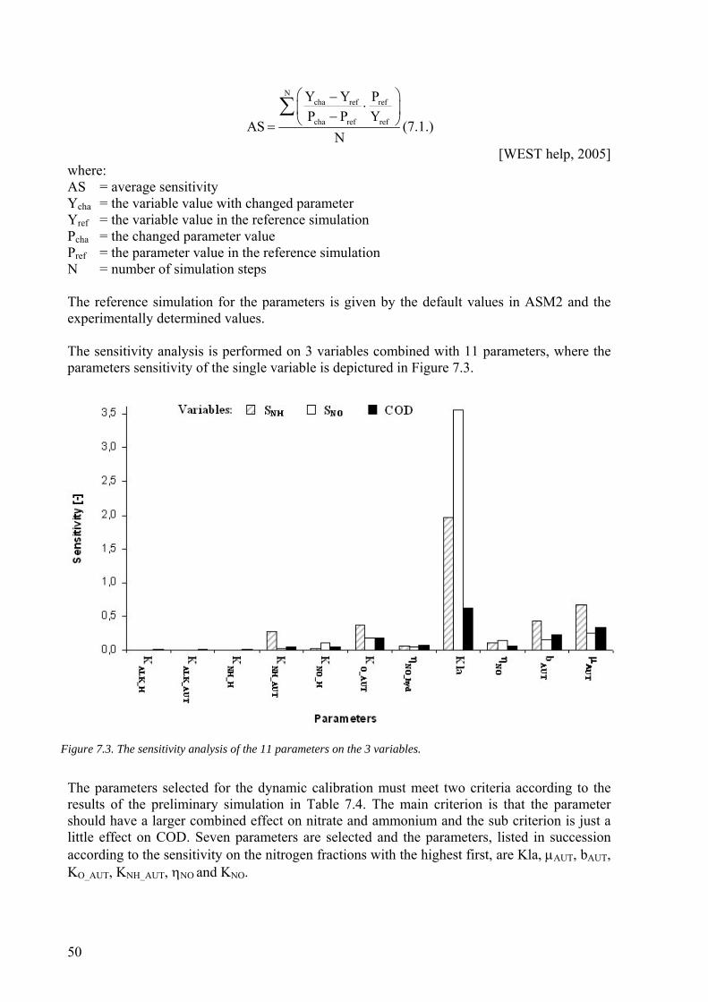
Ncha refY Y P⎛ − ref

f

⎞⋅⎜ ⎟

⎠ (7.1.)

[WEST help, 2005]

cha eter

ref = the parameter value in the reference simulation N = number of simulation steps The reference simulation for the parameters is given by the default values in ASM2 and the experimentally determined values. The sensitivity analysis is performed on 3 variables combined with 11 parameters, where the parameters sensitivity of the single variable is depictured in Figure 7.3.

cha ref reP P YAS

N−⎝=

∑

where: AS = average sensitivity

= the variable value with changed paramYYref = the variable value in the reference simulation Pcha = the changed parameter value P

F 11 parameters on the 3 variables.

The parameters selected for the dynamic calibration must meet two criteria according to the results of the preliminary simulation in Table 7.4. The main criterion is that the parameter should have a larger combined effect on nitrate and ammonium and the sub criterion is just a little effect on COD. Seven parameters are selected and the parameters, listed in succession according to the sensitivity on the nitrogen fractions with the highest first, are Kla, µAUT, bAUT, KO_AUT, KNH_AUT, ηNO and KNO.

igure 7.3. The sensitivity analysis of the

50

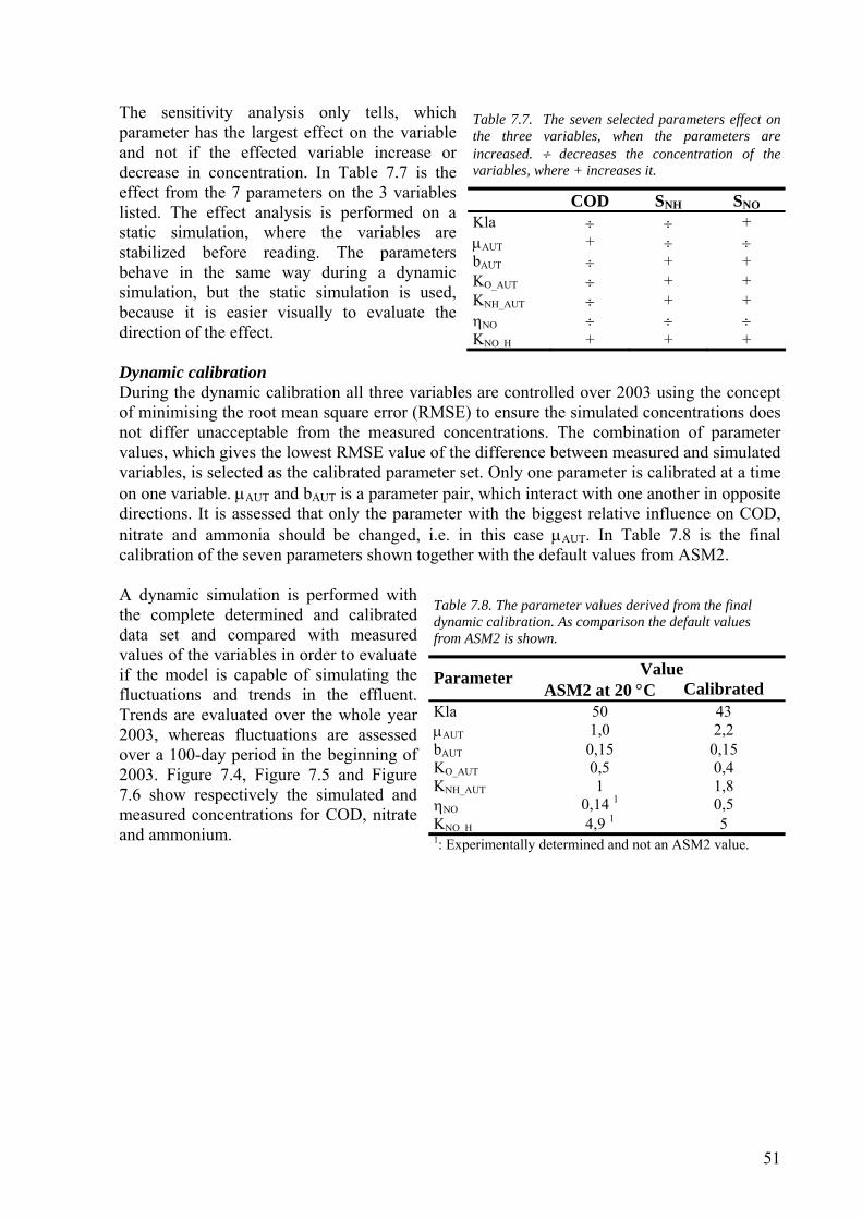
The sensitivity analysis only tells, which parameter has the largest effect on the variable and not if the effected variable increase or decrease in concentration. In Table 7.7 is the effect from the 7 parameters on the 3 variables listed. The effect analysis is performed on a static simulation, where the variables are stabilized before reading. The parameters behave in the same way during a dynamic simulation, but the static simulation is used, because it is easier visually to evaluate the direction of the effect.

Table 7.7. The seven selected parameters effect on the three variables, when the parameters are increased. ÷ decreases the concentration of the variables, where + increases it.

COD SNH SNOKla ÷ ÷ + µAUT + ÷ ÷

bAUT ÷ + + KO_AUT ÷ + + KNH_AUT ÷ + + ηNO ÷ ÷ ÷ KNO_H + + +

Dynamic calibration During the dynamic calibration all three variables are controlled over 2003 using the concept of minimising the root mean square error (RMSE) to ensure the simulated concentrations does not differ unacceptable from the measured concentrations. The combination of parameter values, which gives the lowest RMSE value of the difference between measured and simulated variables, is selected as the calibrated parameter set. Only one parameter is calibrated at a time on one variable. µAUT and bAUT is a parameter pair, which interact with one another in opposite directions. It is assessed that only the parameter with the biggest relative influence on COD, nitrate and ammonia should be changed, i.e. in this case µAUT. In Table 7.8 is the final calibration of the seven parameters shown together with the default values from ASM2. A dynamic simulation is performed with the complete determined and calibrated data set and compared with measured values of the variables in order to evaluate if the model is capable of simulating the fluctuations and trends in the effluent. Trends are evaluated over the whole year 2003, whereas fluctuations are assessed over a 100-day period in the beginning of 2003. Figure 7.4, Figure 7.5 and Figure 7.6 show respectively the simulated and measured concentrations for COD, nitrate and ammonium.

Table 7.8. The parameter values derived from the final dynamic calibration. As comparison the default values from ASM2 is shown.

Value Parameter ASM2 at 20 °C Calibrated

Kla 50 43 µAUT 1,0 2,2 bAUT 0,15 0,15 KO_AUT 0,5 0,4 KNH_AUT 1 1,8 ηNO 0,14 1 0,5 KNO_H 4,9 1 5 1: Experimentally determined and not an ASM2 value.

51

MeasuredSimulated

Time [d]36034032030028026024022020018016014012010080604020

CO

D [m

g/L]

340

320

300

280

260

240

220

200

180

160

140

120

100

80

60

40

MeasuredSimulated

Time [d]9590858075706560555045403530252015105

CO

D [m

g/L]

340

320

300

280

260

240

220

200

180

160

140

120

100

80

60

40

MeasuredSimulated

Time [d]36034032030028026024022020018016014012010080604020

Nitr

ate

[mg/

L]

24

22

20

18

16

14

12

10

8

6

4

2

MeasuredSimulated

Time [d]9590858075706560555045403530252015105

Nitr

ate

[mg/

L]

24

22

20

18

16

14

12

10

8

6

4

2

Figure 7.4. Results of measured COD concentrations in the effluent from the new works in 2003 and the simulation based on the final calibration.

Figure 7.5. Results of measured nitrate concentrations in the effluent from the new works in 2003 and the simulation based on the final calibration.

52

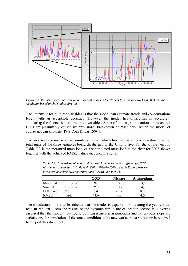
MeasuredSimulated

Time [d]36034032030028026024022020018016014012010080604020

Amm

oniu

m [m

g/L]

32

30

28

26

24

22

20

18

16

14

12

10

8

6

4

2

MeasuredSimulated

Time [d]9590858075706560555045403530252015105

Amm

oniu

m [m

g/L]

16

15

14

13

12

11

10

9

8

7

6

5

4

3

2

1

Figure 7.6. Results of measured ammonium concentrations in the effluent from the new works in 2003 and the simulation based on the final calibration.

The statement for all three variables is that the model can estimate trends and concentrations levels with an acceptable accuracy. However the model has difficulties in accurately simulating the fluctuations of the three variables. Some of the large fluctuations in measured COD are presumably caused by provisional breakdown of machinery, which the model of course not can simulate [Pers.Com.Dildar, 2004]. The area under a measured or simulated curve, which has the daily mass as ordinate, is the total mass of the three variables being discharged to the Umbilo river for the whole year. In Table 7.9 is the measured mass load vs. the simulated mass load to the river for 2003 shown together with the achieved RMSE values on concentrations.

Table 7.9. Comparison of measured and simulated mass load in effluent for COD, nitrate and ammonium in 2003 with −= ⋅Meas. Sim.

Sim.iff . 100% . The RMSE are betwmeasured and simulated concentrations [CD-RO

D een M annex 7].

COD Nitrate Ammonium Measured [Ton/year] 260 10,6 13,0 Simulated [Ton/year] 259 10,7 14,3 Difference [%] 0,4 -0,3 8,7 RMSE [mg/L] 41,6 4,3 4,5

The calculations in the table indicate that the model is capable of simulating the yearly mass load in effluent. From the results of the dynamic run in the calibration section it is overall assessed that the model input found by measurements, assumptions and calibrations steps are satisfactory for simulation of the actual condition at the new works, but a validation is required to support this statement.

53

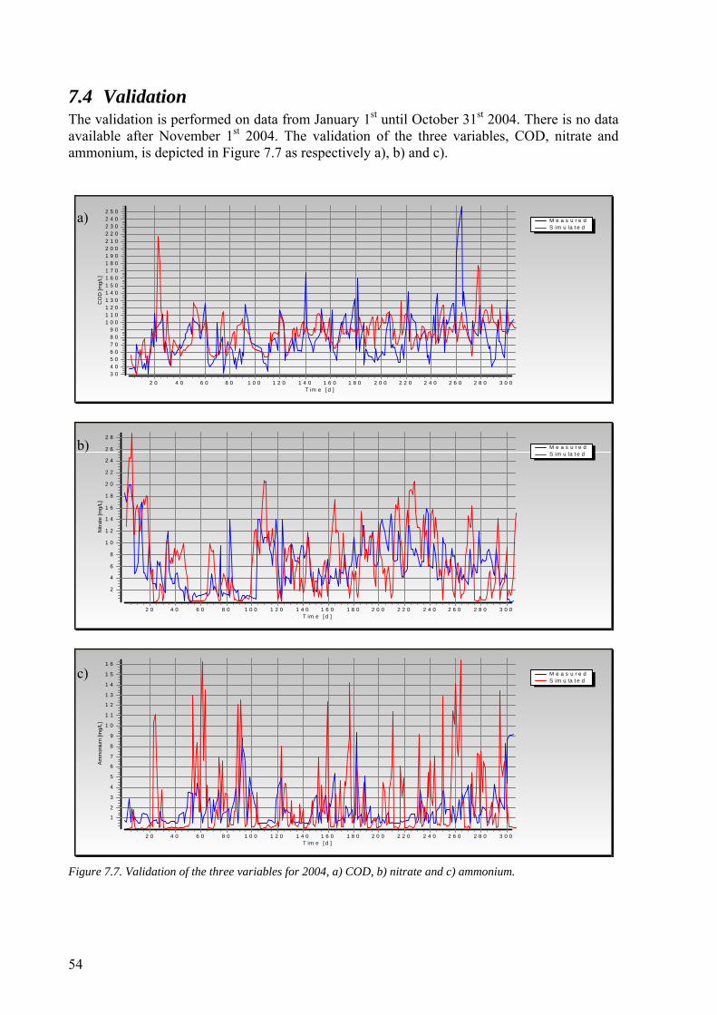
7.4 Validation The validation is performed on data from January 1st until October 31st 2004. There is no data available after November 1st 2004. The validation of the three variables, COD, nitrate and ammonium, is depicted in Figure 7.7 as respectively a), b) and c).

M e a s u r e dS im u la t e d

T im e [ d ]3 0 02 8 02 6 02 4 02 2 02 0 01 8 01 6 01 4 01 2 01 0 08 06 04 02 0

CO

D [m

g/L]

2 5 02 4 02 3 02 2 02 1 02 0 01 9 01 8 01 7 01 6 01 5 01 4 01 3 01 2 01 1 01 0 0

9 08 07 06 05 04 03 0

M e a s u r e dS im u la t e d

T im e [ d ]3 0 02 8 02 6 02 4 02 2 02 0 01 8 01 6 01 4 01 2 01 0 08 06 04 02 0

Nitr

ate

[mg/

L]

2 8

2 6

2 4

2 2

2 0

1 8

1 6

1 4

1 2

1 0

8

6

4

2

M e a s u r e dS im u la t e d

a)

b)

T im e [ d ]3 0 02 8 02 6 02 4 02 2 02 0 01 8 01 6 01 4 01 2 01 0 08 06 04 02 0

1 6

1 3

1 2

Amm

oniu

m [m

g/L]

1 1

1 0

9

8

7

6

5

4

3

2

1

1 5

1 4c)

Figure 7.7. Validation of the three variables for 2004, a) COD, b) nitrate and c) ammonium.

54

During the first validation run the simulated concentrations of ammonium and nitrate shows

erators broke down June 23 2004 representing the 174 day in the simulation period. The 3 remaining own in table 3.1. The va o 47 d-1 after 174th Figure 7.7 a) and b) shows, that odel can estimate the trends and fluctuations of COD and nitrate ) shows odel estimates the trends of ammonium acceptable, th ions are erally es d too h The simulated concentrati e uctuations milar or smaller than the ured. Based on

ese assess oncluded that the va les can be accepted.

of measured and simulated mass load in effluent for COD, in the validation period in 2004.

respectively an in- and decreasing trend after app. 180 days, whereas the measured concentration does not display this trend. Previous investigation revealed that one of the

rd thaaerators compensates for this by increasing the total aeration time as shlidation reproduces this situation by increasing the Kla value from 43 tdays as shown in the figures above.

the m acceptable. Figure 7.7 c

uctuat, that the m

however etw

e fl gen t teima igh. ons in bments it is c

en the fl are silidation for the three variab

measth The model is also accepted based on the measured mass load vs. the simulated mass load to the river for the validation period in Table 7.10, since the values does not deviate significantly.

Table 7.10. Comparisonnitrate and ammonium Meas. Sim.

Sim.Diff . 100%−= ⋅ . The

COD Nitrate Ammonium

RMSE are between measured and simulated concentrations [CD-ROM annex 7].

Measured [Ton/year] 177 13,1 4,1 Simulated [Ton/year] 195 13,1 3,9 Difference [%] 10,0 0,0 -5,2 RMSE [mg/L] 38,3 4,3 3,7

Both results from the calibration and validation conclude that the model can simulate trends and average COD, nitrate and ammonium mass loads at the new works. The limitation of the model is that actual fluctuations in the effluent cannot be simulated accurately. Based on the pros and cons, the model can show if an optimizing initiative causes an in- or decrease in the concentrations in the effluent. The model is therefore in the subsequently chapter used as a tool for optimizing the processes for COD and ammonium removal.

55

8 Optimization of the CSTR at USPW The purpose of the optimization is to investigate the effect of four different scenarios on COD and ammonium concentrations in the effluent from the new works using the WEST model and the dynamic input file from 2003. There is no discharge demand on nitrate and it is therefore not assessed in the optimization process. The optimization of COD removal must not have an increasing impact on the concentration of ammonium in the effluent and visa versa. The scenarios are chosen, based on what the authors assume is economically viable at the new works, this means the optimization does not include drastically plant design alterations. The four different scenarios are:

1. The oxygen concentration in the CSTR is raised. 2. The sludge concentration in the CSTR is increased 3. The sludge age in the CSTR is increased 4. The present design of the CSTR is converted to a traditional design with anoxic

and aerobic tank together with a nitrate recycle. The effect of any optimization initiative is assessed by comparing the present simulated average discharge concentrations of COD and ammonium, which respectively are 92 mg O2/L and 4,4 mg N/L, with the optimized average concentrations. The following sections consist of a theoretical description of the individual scenarios followed by a summary of the achieved optimizing results.

8.1 The oxygen concentration in the CSTR is raised In this scenario is the oxygen concentration in the CSTR raised by increasing the oxygen transfer coefficient, Kla. The average oxygen concentration is simulated at 0,2 mg O2/L with the present calibrated configuration. The Kla value is increased until the value corresponds to an average oxygen concentrations of 2 mg O2/L. Raising the oxygen concentration further than 2 mg O2/L seldom results in process-technical advantages, because higher oxygen concentration inhibits the simultaneously denitrification process [Randall et al., 1992]. The increase in Kla represents an increase in the total operating hours of the four aerators. The raised oxygen concentration increases the reaction rate for any reaction with the monod equation for oxygen, i.e. aerobic hydrolysis, aerobic growth of heterotrophic and autotrophic biomass, provided that the reactions are only limited by the oxygen concentration. The growth of the biomass converts soluble COD to particulate COD as biomass, whereas the hydrolysis does just the opposite. The model is used to assess the overall effect on the COD concentration in the effluent. The autotrophic biomass performs nitrification and an increase in the oxygen concentration decreases the ammonium concentration in the effluent on the expense of an increase in the nitrate concentration.

8.2 The sludge concentration in the CSTR is increased In this scenario is the sludge concentration in the CSTR increased by raising the return sludge flow rate from the two secondary settlers. The concentration in the CSTR will approach the concentration in underflow from the two secondary settlers, when the return flow rate is increased. The concentration in the junction point between the return flow and the overflow from the primary clarifier is calculated from equation 8.1 based on the notation in figure B.2 in

56

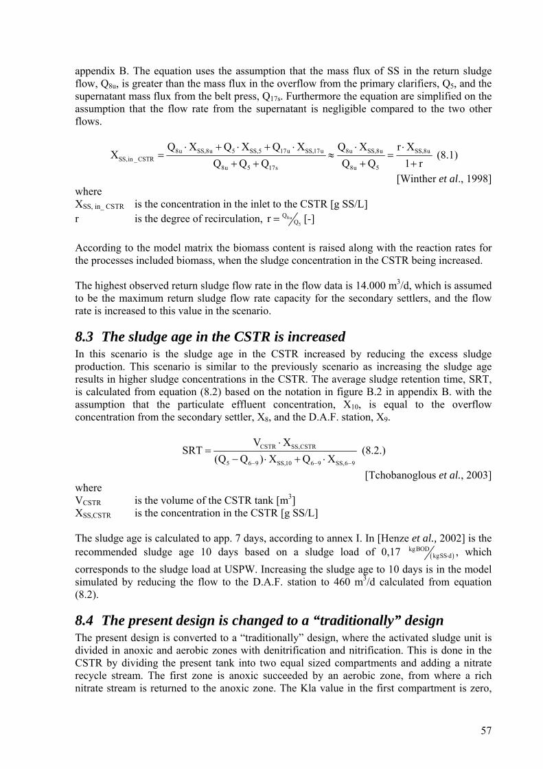
appendix B. The equation uses the assumption that the mass flux of SS in the return sludge flow, Q8u, is greater than the mass flux in the overflow from the primary clarifiers, Q5, and the supernatant mass flux from the belt press, Q17s. Furthermore the equation are simplified on the assumption that the flow rate from the supernatant is negligible compared to the two other flows.

8u SS,8u 5 SS,5 17u SS,17u 8u SS,8u SS,8uSS,in _ CSTR

8u 5 17s 8u 5

Q X Q X Q X Q X r XX

Q Q Q Q Q 1 r⋅ + ⋅ + ⋅ ⋅ ⋅

= ≈+ + + +

= (8.1)

[Winther et al., 1998] where XSS, in_ CSTR is the concentration in the inlet to the CSTR [g SS/L] r is the degree of recirculation, 8uQ=

5Qr [-] According to the model matrix the biomass content is raised along with the reaction rates for he processes included biomass, when the sludge concentration in the CSTR being increased. t

The highest observed return sludge flow rate in the flow data is 14.000 m3/d, which is assumed to be the maximum return sludge flow rate capacity for the secondary settlers, and the flow rate is increased to this value in the scenario.

8.3 The sludge age in the CSTR is increased In this scenario is the sludge age in the CSTR increased by reducing the excess sludge production. This scenario is similar to the previously scenario as increasing the sludge age results in higher sludge concentrations in the CSTR. The average sludge retention time, SRT, is calculated from equation (8.2) based on the notation in figure B.2 in appendix B. with the assumption that the particulate effluent concentration, X10, is equal to the overflow oncentration from the secondary settler, Xc

8, and the D.A.F. station, X9.

CSTR SS,CSTR

5 6 9 SS,10 6 9 SS,6

V XSRT

(Q Q ) X Q X 9− − −

⋅=

− ⋅ + ⋅ (8.2.)

[Tchobanoglous et al., 2003] where VCSTR is the volume of the CSTR tank [m ] 3

XSS,CSTR is the concentration in the CSTR [g SS/L] The sludge age is calculated to app. 7 days, according to annex I. In [Henze et al., 2002] is the recommended sludge age 10 days based on a sludge load of 0,17 ( )

kgBODkgSS d⋅ , which

corresponds to the sludge load at USPW. Increasing the sludge age to 10 days is in3

the model simulated by reducing the flow to the D.A.F. station to 460 m /d calculated from equation

one. The Kla value in the first compartment is zero,

(8.2).

8.4 The present design is changed to a “traditionally” design The present design is converted to a “traditionally” design, where the activated sludge unit is divided in anoxic and aerobic zones with denitrification and nitrification. This is done in the CSTR by dividing the present tank into two equal sized compartments and adding a nitrate recycle stream. The first zone is anoxic succeeded by an aerobic zone, from where a rich nitrate stream is returned to the anoxic z

57

which corresponds to an anoxic zone. In the second compartment is the Kla value adjusted to

s at USPW does therefore not require external carbon source. Based on the ratio the scenario has a realistic

dditional operating costs.

n with specification of the duction in COD and ammonium concentrations. The calculations of the reduction of COD

Table 8.1. Reduction in simula mmonium concentrations in the effluent achieved by the four s initiativ g/L]. [C

duc

an oxygen concentration of 2 mg O2/L. [Jansen et al., 2000] states that the recycle flow rate is normally a factor 2 – 5 of the influent flow rate, hence a nitrate recycle flow rate of 20.000 m3/d is chosen in the model. As previous stated in section 4.1.2, the COD/TN ratio is high and the denitrification proces

perspective and the process is not associated with a

8.5 Results from the four scenarios In Table 8.1 are the results from the four optimizing scenarios showreand ammonium for each scenario are listed in CD-ROM annex 6.

ted COD and ancentration unoptimization e. The co it is [m D-ROM annex 6]

Re tion COD NH4

+Scenario C . Co .

-1

to

onc % nc % Additional information

The dissolved oxygen concentration in the CSTR is 2,3 mg O /L with1 11 12 4 92 2 a Kla of 95 d . The average nitrate concentration is raised from 4,4 mg N/L23 mg N/L.

2 0 0 0 0 The COD concentration in the CSTR remains unchanged at app. 2.090 mg/L

3 4 4 0,4 8 The COD concentration in CSTR is raised from app. 2.090 mg/L to app. 3.000 mg/L

4 -2,9 1 -3 1 4,3 97 The overall mass of nitrogen is reduced by 56 % or 14 tones nitrogen per year.

1: The value is negative thus an increase. In scenario 1 is the oxygen concentration raised from 0,2 mg O2/L to 2,3 mg O2/L, which results in a 12 % reduction of the COD effluent concentration. Ammonium is almost completely removed from the effluent, however it is on the expense of the nitrate concentration as it increases significantly. Scenario 2 has no effect on either the COD or ammonium concentration in the effluent, which was not expected according to the theory. The purpose of scenario 3 is to increase the sludge age to 10 days. After the excess production is reduced, the COD concentration in the CSTR is raised to 3.000 mg/L (≈ 2.560 mg SS/L) and the sludge age is 10,4 days. This causes a reduction of 4 mg COD/L in the COD concentration in the effluent, whereas the ammonium concentration is almost unaffected. Scenario 4 have a significant impact on ammonium concentration and the overall mass of nitrogen discharged in

e effluent, as the mass is reduced with 14 tones nitrogen per year or app. 50 %. The scenario

ctively 11 mg COD/L and 4

thdoes however cause an increase in the COD concentration of 2,9 mg/L or 3 %. Scenario 1 and 3 are the only scenarios of the four, where the effluent concentrations of COD and ammonium are reduced. The two scenarios are combined in scenario 5 to investigate the combined effect on COD and ammonium removal. Scenario 2 and 4 are not selected, because they have very little or increasing effect on the COD concentration in the effluent. Scenario 5 shows a reduction of COD and ammonium in the effluent of respe

58

mg N/L. This is identically with the reduction achieved in scenario 1 and since no combined

ized onfiguration is implemented, means for the new works compliance with the legislation. As

also chieved on measurements, when the optimized configuration is implemented in the plant.

Table 8.2 show nd ammonium in the effluent from t timization.

Table 8.2. The reduction t ve opt me imp e for C

Concentration of Time compliance of

effect is achieved only Kla is changed in the subsequent section.

8.6 The effect on legislation with the optimized configuration This section investigates, what the reduction in COD and ammonium, when the optimcstated in section 4.2, the new works does currently not have any discharge demands, but it was assumed that the discharge demands for the old works would apply to the new works also It is assumed that the same reduction achieved with the optimized configuration is a

s the previous average measured concentration of COD ahe new works and the estimated effluent concentration after op

in the measured efflueni onfigur n s i

alues of COD and ple at the ammonium, when th

works along with thmized croved tim

atio iplianc

mented OD and

new nium. e com ammo

COD C Ntion [%]

Present 93 4,0 84 88

NH4+ OD H4

+Configura[mg/L]

Optimized 82 1 1,8 1 89 95 1: Daily measured values subtracted the expected reduction

The time compliance for COD and ammonium is improved, when the optimized configuration is implemented with an average oxygen concentration in the CSTR of 2,3 mg O2/L. If this

crease in efficiency and time compliance with the legislation is satisfactory for Durban etropolitan and USPW, it is then recommended to install oxygen probes in the CSTR with aintaining an oxygen concentration of app. 2 mg O2/L in mind.

inMm

59

9 Maximum allowed discharge of heavy metals The purpose of this chapter is to recommend the maximum allowed discharge of heavy metals concentrations from the industry, where Umbilo Sewage Purification works (USPW) still is in compliance with the legislation. The heavy metals from the metal finishing and textile companies in the catchment area are removed primarily through the sludge. A mass balance, where the actual sludge concentrations are substituted with the allowed concentrations, is used to estimate the maximum allowed quantity of heavy metals from the industry. Sludge can be disposed in three different ways with three different guidelines and minimum requirements for the sludge:

• Sludge disposed on-site at the treatment plant • Sludge dumped at sea • Sludge used for agricultural purposes.

The minimum requirements for sludge disposed on-site are based on the potential danger (carcinogenicity, mutagenicity, teratogenicity, etc.) of each component in the sludge. The actual concentration in the sludge of each compound is compared to an acceptable risk level calculated as 10% of the LC50. LC50 is the concentration at which a substance would kill 50 per cent of organisms if it were disposed of directly into a body of water. If the concentration of the hazardous substance is only ten percent of the LC50, it should have very little harmful effect on the aquatic. The actual concentration in the sludge has to be lower than the acceptable risk level. [DWAF, 1998] The marine disposal of sludge is assigned to the same minimum requirements. [DWAF, 2004] The Department of Water Affairs and Forestry in South Africa do not recommend the two disposal types above as long term solutions for the disposal of sewage sludge, contrary to sludge being used for agricultural purposes. The following sections deals with the scenario; what the requirements for sludge from USPW would be, if the sludge were used for agricultural purposes.

9.1 Requirements for sludge used for agricultural purposes In addition to that USPW has to comply with the General Standards for the effluent, the plant also has to comply with the Permissible Utilization and Disposal of Sewage Sludge (PUDSS) law for the sludge produced at the plant. Section (4.2) discussed the quality of the effluent, whereas this section also evaluates the quality of the sludge with reference to a possible disposal and utilization of the sludge. In order for sewage sludge to be disposed and utilized it has to meet certain standards with regards to the content of inorganic components, pathogenic organisms and the sludge’s potential for odour and fly-breeding problems as stated in PUDSS from 1997 [DWAF, 1997]. This section will only investigate the heavy metals content in the sludge, as there are only measurements of metal concentrations in the sludge available.

9.1.1 Discharge standards of sludge and effluent for heavy metals On the basis of the industries in the catchment area USPW selects to measure eight different heavy metals. Table 9.1 shows the heavy metals concentrations for the General Standards for effluent, PUDSS standards for sludge and city-by laws for industries [Pers.Com. Fennemore, 2004].

60

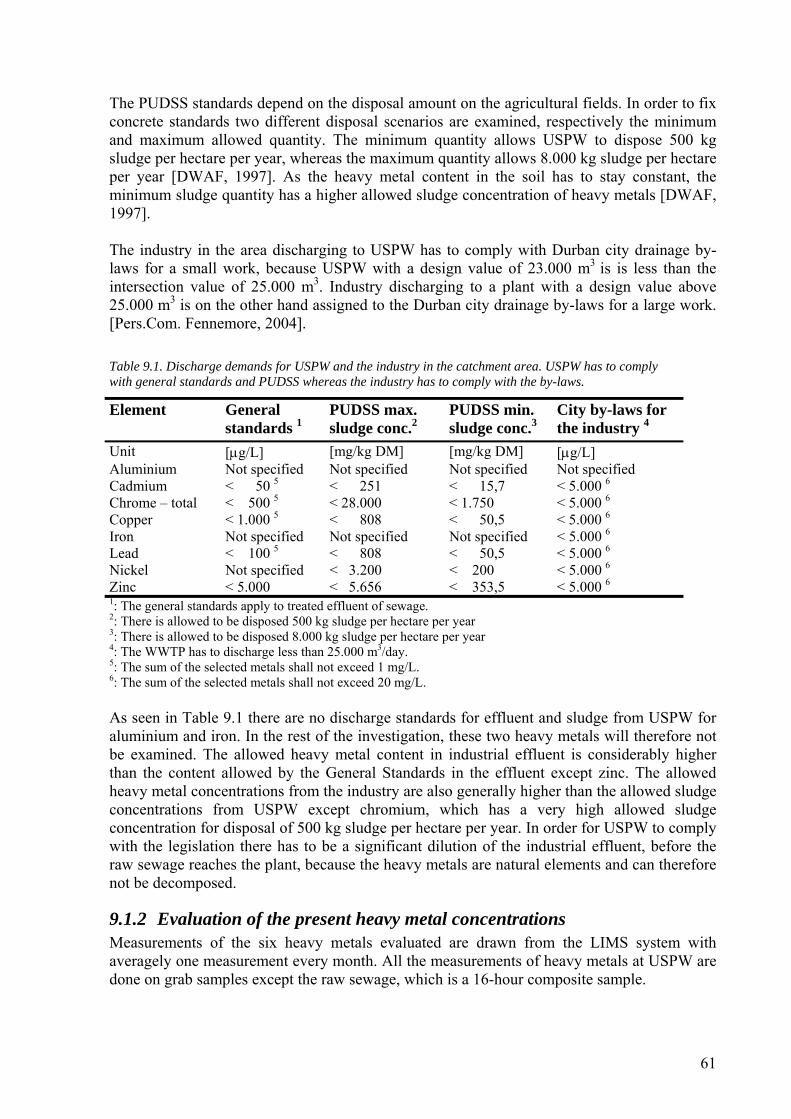
The PUDSS standards depend on the disposal amount on the agricultural fields. In order to fix concrete standards two different disposal scenarios are examined, respectively the minimum and maximum allowed quantity. The minimum quantity allows USPW to dispose 500 kg sludge per hectare per year, whereas the maximum quantity allows 8.000 kg sludge per hectare per year [DWAF, 1997]. As the heavy metal content in the soil has to stay constant, the minimum sludge quantity has a higher allowed sludge concentration of heavy metals [DWAF, 1997]. The industry in the area discharging to USPW has to comply with Durban city drainage by-laws for a small work, because USPW with a design value of 23.000 m3 is is less than the intersection value of 25.000 m3. Industry discharging to a plant with a design value above 25.000 m3 is on the other hand assigned to the Durban city drainage by-laws for a large work. [Pers.Com. Fennemore, 2004]. Table 9.1. Discharge demands for USPW and the industry in the catchment area. USPW has to comply with general standards and PUDSS whereas the industry has to comply with the by-laws.

Element General standards 1

PUDSS max. sludge conc.2

PUDSS min. sludge conc.3

City by-laws for the industry 4

Unit [µg/L] [mg/kg DM] [mg/kg DM] [µg/L] Aluminium Not specified Not specified Not specified Not specified Cadmium < 50 5 < 251 < 15,7 < 5.000 6Chrome – total < 500 5 < 28.000 < 1.750 < 5.000 6Copper < 1.000 5 < 808 < 50,5 < 5.000 6Iron Not specified Not specified Not specified < 5.000 6Lead < 100 5 < 808 < 50,5 < 5.000 6Nickel Not specified < 3.200 < 200 < 5.000 6Zinc < 5.000 < 5.656 < 353,5 < 5.000 61: The general standards apply to treated effluent of sewage. 2: There is allowed to be disposed 500 kg sludge per hectare per year 3: There is allowed to be disposed 8.000 kg sludge per hectare per year 4: The WWTP has to discharge less than 25.000 m3/day. 5: The sum of the selected metals shall not exceed 1 mg/L. 6: The sum of the selected metals shall not exceed 20 mg/L. As seen in Table 9.1 there are no discharge standards for effluent and sludge from USPW for aluminium and iron. In the rest of the investigation, these two heavy metals will therefore not be examined. The allowed heavy metal content in industrial effluent is considerably higher than the content allowed by the General Standards in the effluent except zinc. The allowed heavy metal concentrations from the industry are also generally higher than the allowed sludge concentrations from USPW except chromium, which has a very high allowed sludge concentration for disposal of 500 kg sludge per hectare per year. In order for USPW to comply with the legislation there has to be a significant dilution of the industrial effluent, before the raw sewage reaches the plant, because the heavy metals are natural elements and can therefore not be decomposed.

9.1.2 Evaluation of the present heavy metal concentrations Measurements of the six heavy metals evaluated are drawn from the LIMS system with averagely one measurement every month. All the measurements of heavy metals at USPW are done on grab samples except the raw sewage, which is a 16-hour composite sample.

61

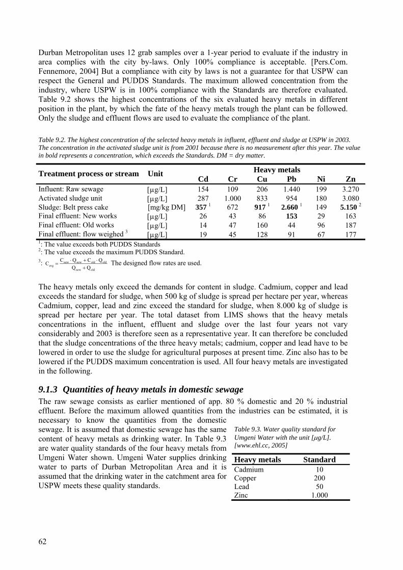
Durban Metropolitan uses 12 grab samples over a 1-year period to evaluate if the industry in area complies with the city by-laws. Only 100% compliance is acceptable. [Pers.Com. Fennemore, 2004] But a compliance with city by laws is not a guarantee for that USPW can respect the General and PUDDS Standards. The maximum allowed concentration from the industry, where USPW is in 100% compliance with the Standards are therefore evaluated. Table 9.2 shows the highest concentrations of the six evaluated heavy metals in different position in the plant, by which the fate of the heavy metals trough the plant can be followed. Only the sludge and effluent flows are used to evaluate the compliance of the plant. Table 9.2. The highest concentration of the selected heavy metals in influent, effluent and sludge at USPW in 2003. The concentration in the activated sludge unit is from 2001 because there is no measurement after this year. The value in bold represents a concentration, which exceeds the Standards. DM = dry matter.

Heavy metals Treatment process or stream Unit Cd Cr Cu Pb Ni Zn

Influent: Raw sewage [µg/L] 154 109 206 1.440 199 3.270 Activated sludge unit [µg/L] 287 1.000 833 954 180 3.080 Sludge: Belt press cake [mg/kg DM] 357 1 672 917 1 2.660 1 149 5.150 2Final effluent: New works [µg/L] 26 43 86 153 29 163 Final effluent: Old works [µg/L] 14 47 160 44 96 187 Final effluent: flow weighed 3 [µg/L] 19 45 128 91 67 177 1: The value exceeds both PUDDS Standards

2: The value exceeds the maximum PUDDS Standard. 3: new new old old

avgnew old

C Q C QCQ Q

⋅ + ⋅=

+ The designed flow rates are used.

The heavy metals only exceed the demands for content in sludge. Cadmium, copper and lead exceeds the standard for sludge, when 500 kg of sludge is spread per hectare per year, whereas Cadmium, copper, lead and zinc exceed the standard for sludge, when 8.000 kg of sludge is spread per hectare per year. The total dataset from LIMS shows that the heavy metals concentrations in the influent, effluent and sludge over the last four years not vary considerably and 2003 is therefore seen as a representative year. It can therefore be concluded that the sludge concentrations of the three heavy metals; cadmium, copper and lead have to be lowered in order to use the sludge for agricultural purposes at present time. Zinc also has to be lowered if the PUDDS maximum concentration is used. All four heavy metals are investigated in the following.

9.1.3 Quantities of heavy metals in domestic sewage The raw sewage consists as earlier mentioned of app. 80 % domestic and 20 % industrial effluent. Before the maximum allowed quantities from the industries can be estimated, it is necessary to know the quantities from the domestic sewage. It is assumed that domestic sewage has the same content of heavy metals as drinking water. In Table 9.3 are water quality standards of the four heavy metals from Umgeni Water shown. Umgeni Water supplies drinking water to parts of Durban Metropolitan Area and it is assumed that the drinking water in the catchment area for USPW meets these quality standards.

Table 9.3. Water quality standard for Umgeni Water with the unit [µg/L]. [www.ehl.cc, 2005]

Heavy metals Standard Cadmium 10 Copper 200 Lead 50 Zinc 1.000

62

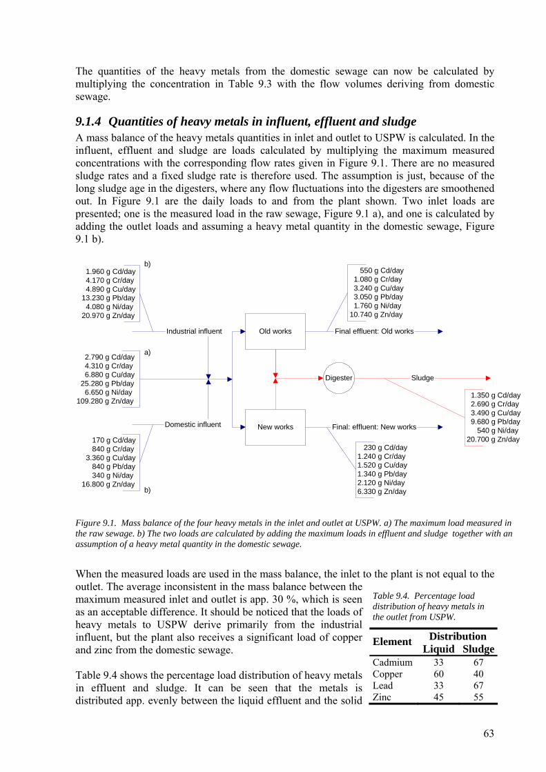
The quantities of the heavy metals from the domestic sewage can now be calculated by multiplying the concentration in Table 9.3 with the flow volumes deriving from domestic sewage.

9.1.4 Quantities of heavy metals in influent, effluent and sludge A mass balance of the heavy metals quantities in inlet and outlet to USPW is calculated. In the influent, effluent and sludge are loads calculated by multiplying the maximum measured concentrations with the corresponding flow rates given in Figure 9.1. There are no measured sludge rates and a fixed sludge rate is therefore used. The assumption is just, because of the long sludge age in the digesters, where any flow fluctuations into the digesters are smoothened out. In Figure 9.1 are the daily loads to and from the plant shown. Two inlet loads are presented; one is the measured load in the raw sewage, Figure 9.1 a), and one is calculated by adding the outlet loads and assuming a heavy metal quantity in the domestic sewage, Figure 9.1 b).

1.960 g Cd/day 4.170 g Cr/day 4.890 g Cu/day13.230 g Pb/day 4.080 g Ni/day20.970 g Zn/day

170 g Cd/day 840 g Cr/day 3.360 g Cu/day 840 g Pb/day 340 g Ni/day16.800 g Zn/day

Old works

New works

Digester

Final: effluent: New works

Final effluent: Old worksIndustrial influent

Domestic influent

Sludge

550 g Cd/day 1.080 g Cr/day 3.240 g Cu/day 3.050 g Pb/day 1.760 g Ni/day10.740 g Zn/day

230 g Cd/day1.240 g Cr/day1.520 g Cu/day1.340 g Pb/day2.120 g Ni/day6.330 g Zn/day

1.350 g Cd/day 2.690 g Cr/day 3.490 g Cu/day 9.680 g Pb/day 540 g Ni/day20.700 g Zn/day

2.790 g Cd/day 4.310 g Cr/day 6.880 g Cu/day 25.280 g Pb/day 6.650 g Ni/day109.280 g Zn/day

a)

b)

b)

Figure 9.1. Mass balance of the four heavy metals in the inlet and outlet at USPW. a) The maximum load measured in the raw sewage. b) The two loads are calculated by adding the maximum loads in effluent and sludge together with an assumption of a heavy metal quantity in the domestic sewage.

When the measured loads are used in the mass balance, the inlet to the plant is not equal to the outlet. The average inconsistent in the mass balance between the maximum measured inlet and outlet is app. 30 %, which is seen as an acceptable difference. It should be noticed that the loads of heavy metals to USPW derive primarily from the industrial influent, but the plant also receives a significant load of copper and zinc from the domestic sewage. Table 9.4 shows the percentage load distribution of heavy metals in effluent and sludge. It can be seen that the metals is

Table 9.4. Percentage load distribution of heavy metals in the outlet from USPW.

Distribution Element Liquid Sludge

Cadmium 33 67 Copper 60 40 Lead 33 67 Zinc 45 55 distributed app. evenly between the liquid effluent and the solid

63

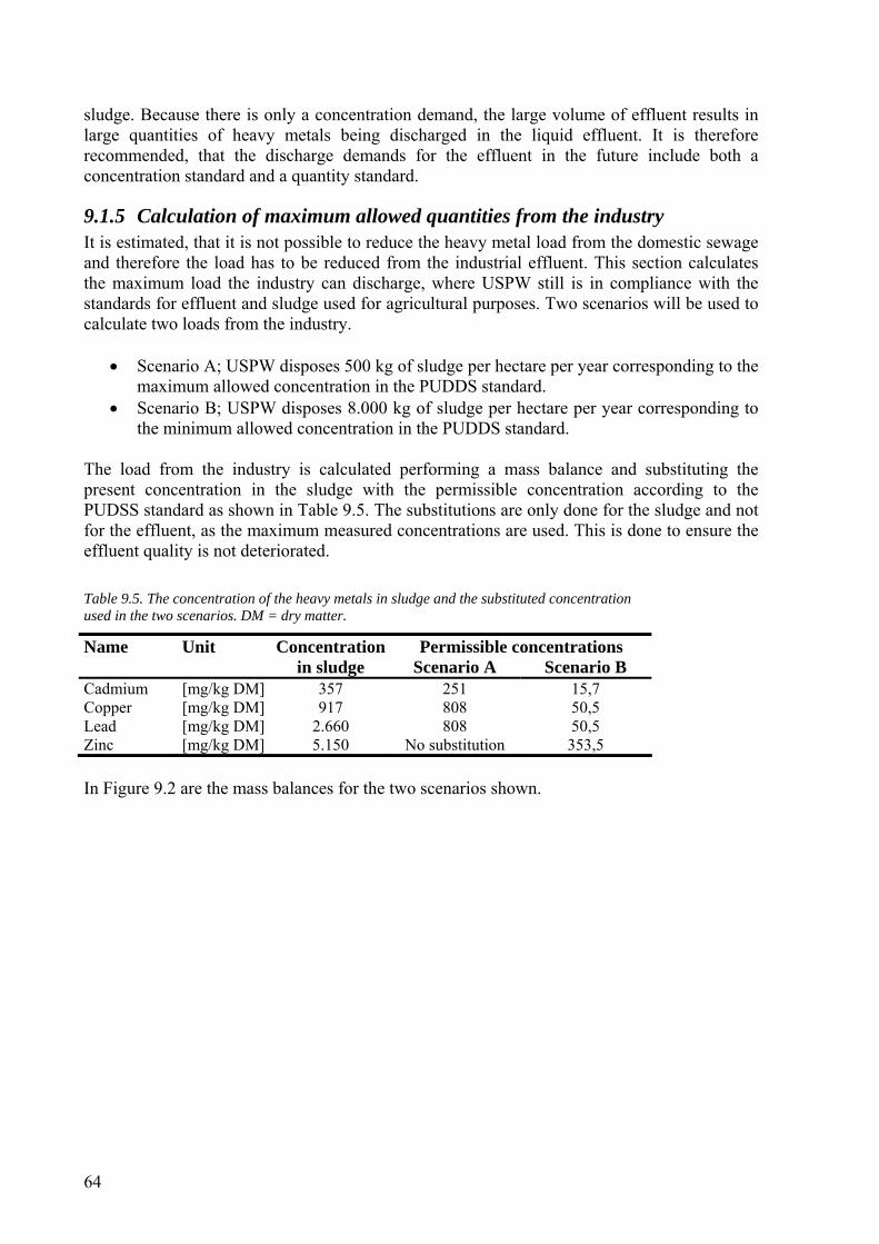
sludge. Because there is only a concentration demand, the large volume of effluent results in large quantities of heavy metals being discharged in the liquid effluent. It is therefore recommended, that the discharge demands for the effluent in the future include both a concentration standard and a quantity standard.

9.1.5 Calculation of maximum allowed quantities from the industry

• Scenario A; USPW disposes 500 kg of sludge per hectare per year corresponding to the

• re per year corresponding to

he load from the industry is calculated performing a mass balance and substituting the

able 9.5. The concentration of the heavy metals in sludge and the substituted concentration

Permissible concentrations

It is estimated, that it is not possible to reduce the heavy metal load from the domestic sewage and therefore the load has to be reduced from the industrial effluent. This section calculates the maximum load the industry can discharge, where USPW still is in compliance with the standards for effluent and sludge used for agricultural purposes. Two scenarios will be used to calculate two loads from the industry.

maximum allowed concentration in the PUDDS standard. Scenario B; USPW disposes 8.000 kg of sludge per hectathe minimum allowed concentration in the PUDDS standard.

Tpresent concentration in the sludge with the permissible concentration according to the PUDSS standard as shown in Table 9.5. The substitutions are only done for the sludge and not for the effluent, as the maximum measured concentrations are used. This is done to ensure the effluent quality is not deteriorated. Tused in the two scenarios. DM = dry matter.

Name Unit Concentration S

Cadmium [mg/kg DM]in sludge

357 cenario A Scenario B

251 15,7 Copper [mg/kg DM] 917 808 50,5 Lead [mg/kg DM] 2

No substitution .660 808 50,5

Zinc [mg/kg DM] 5.150 353,5 In Figure 9.2 are the mass balances for the two scenarios shown.

64

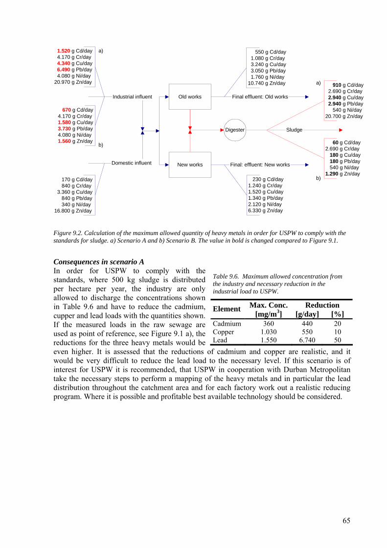
Figure 9.2. Calculation of the maximum allowed quantity of heavy metals in order for USPW to comply with the standards for sludge. a) Scenario A and b) Scenario B. The value in bold is changed compared to Figure 9.1.

1.520 g C

4.3406.490 g

d/day 4.170 g Cr/day

g Cu/day Pb/day

4.080 g Ni/day20.970 g Zn/day

170 g Cd/day 840 g Cr/day 3.360 g Cu/day 840 g Pb/day 340 g Ni/day16.800 g Zn/day

Old works

New works

Digester

Final: effluent: New works

Final effluent: Old worksIndustrial influent

Domestic influent

Sludge

550 g Cd/day 1.080 g Cr/day 3.240 g Cu/day 3.050 g Pb/day 1.760 g Ni/day10.740 g Zn/day

230 g Cd/day1.240 g Cr/day1.520 g Cu/day1.340 g Pb/day2.120 g Ni/day6.330 g Zn/day

60 g Cd/day2.690 g Cr/day 180 g Cu/day 180 g Pb/day 540 g Ni/day1.290 g Zn/day

a)

b)

670 g C

1.580 g C3.730 g

1.560 g Zn

d/day4.170 g Cr/day

u/day Pb/day

4.080 g Ni/day/day

910 g Cd/day 2.690 g Cr/day 2.940 g Cu/day 2.940 g Pb/day 540 g Ni/day20.700 g Zn/day

a)

b)

Consequences in scenario A In order for USPW to comply with the standards, where 500 kg sludge is distributed per hectare per year, the industry are only allowed to discharge the concentrations shown in Table 9.6 and have to reduce the cadmium, cupper and lead loads with the quantities shown. If the measured loads in the raw sewage are used as point of reference, see Figure 9.1 a), the reductions for the three heavy metals would be even higher. It is assessed that the reductions of cadmium and copper are realistic, and it would be very difficult to reduce the lead load to the necessary level. If this scenario is of interest for USPW it is recommended, that USPW in cooperation with Durban Metropolitan take the necessary steps to perform a mapping of the heavy metals and in particular the lead distribution throughout the catchment area and for each factory work out a realistic reducing program. Where it is possible and profitable best available technology should be considered.

Table 9.6. Maximum allowed concentration from the industry and necessary reduction in the industrial load to USPW.

Max. Conc. Reduction Element [mg/m3] [g/day] [%]

Cadmium 360 440 20 Copper 1.030 550 10 Lead 1.550 6.740 50

65

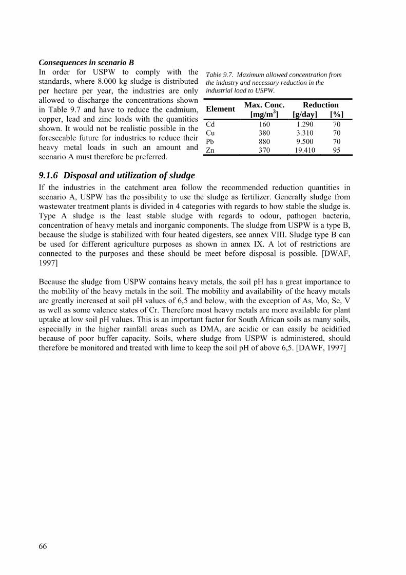
Consequences in scenario B In order for USPW to comply with the standards, where 8.000 kg sludge is distributed per hectare per year, the industries are only allowed to discharge the concentrations shown in Table 9.7 and have to reduce the cadmium, copper, lead and zinc loads with the quantities shown. It would not be realistic possible in the foreseeable future for industries to reduce their heavy metal loads in such an amount and scenario A must therefore be preferred.

Table 9.7. Maximum allowed concentration from the industry and necessary reduction in the industrial load to USPW.

Max. Conc. Reduction Element [mg/m3] [g/day] [%]

Cd 160 1.290 70 Cu 380 3.310 70 Pb 880 9.500 70 Zn 370 19.410 95

9.1.6 Disposal and utilization of sludge If the industries in the catchment area follow the recommended reduction quantities in scenario A, USPW has the possibility to use the sludge as fertilizer. Generally sludge from wastewater treatment plants is divided in 4 categories with regards to how stable the sludge is. Type A sludge is the least stable sludge with regards to odour, pathogen bacteria, concentration of heavy metals and inorganic components. The sludge from USPW is a type B, because the sludge is stabilized with four heated digesters, see annex VIII. Sludge type B can be used for different agriculture purposes as shown in annex IX. A lot of restrictions are connected to the purposes and these should be meet before disposal is possible. [DWAF, 1997] Because the sludge from USPW contains heavy metals, the soil pH has a great importance to the mobility of the heavy metals in the soil. The mobility and availability of the heavy metals are greatly increased at soil pH values of 6,5 and below, with the exception of As, Mo, Se, V as well as some valence states of Cr. Therefore most heavy metals are more available for plant uptake at low soil pH values. This is an important factor for South African soils as many soils, especially in the higher rainfall areas such as DMA, are acidic or can easily be acidified because of poor buffer capacity. Soils, where sludge from USPW is administered, should therefore be monitored and treated with lime to keep the soil pH of above 6,5. [DAWF, 1997]

66

10 Conclusion This project is initiated as a part of the vision from Durban Metropolitan to model each and every wastewater treatment plants in the Durban Metropolitan Area and to reduce the organic and nutrient load to Umbilo river. The new works at Umbilo Sewage Purification Works (USPW) is modelled in the program WEST with the biological treatment processes in the activated sludge unit being modelled in a sub-model. The sub-model is based on the activated sludge model No. 2 but modified to suit the actual conditions in the unit. In order to make the sub-model specific to the USPW 9 parameters are determined from experiments with oxygen uptake rates and nitrate uptake rates. The remaining parameters are determined in a calibration. The calibration on the year 2003 and validation on 2004 of the WEST model for the new works reveals that it can predict trends in effluent concentrations and average effluent loads of the three variables; COD, ammonium and nitrate. However the model is incapable of simulating the fluctuations of the variables in the effluent acceptable. It is overall concluded that the model can be used as a tool to control the average discharge in effluent for the variables and assess the effect of optimizing initiative on the present plant configuration. The COD and ammonium removal from the new works are investigated in 5 different scenarios in order to optimize the efficiency of the treatment processes. Only one scenario gives a significantly reduction in effluent concentration of both variables. The scenario is an increase in the oxygen concentration in the activated sludge unit from 0,2 mg O2/L to 2,3 mg O2/L. This gives a reduction in COD and ammonium concentration of respectively 11 mg COD/L and 4,0 mg N/L. If the above reduction in the average effluent concentration is satisfactory for Durban Metropolitan and USPW, it is recommended for the staff at USPW to increase the overall aeration time for the four surface aerators. Furthermore the recommendation is that oxygen probes should be installed in the activated sludge unit to control and maintain an oxygen level about 2 mg O2/L. The maximum allowed discharge of heavy metals concentrations from the industry, where USPW still is in compliance with the legislation are estimated. The estimation is based on the assumption that USPW can use the sludge for agricultural purposes. In order for USPW to comply with the standards, where 500 kg sludge is distributed per hectare per year, the industry are only allowed to discharge the following concentrations; cadmium 360 mg/m3, copper 1.030 mg/m3 and lead 1.550 mg/m3.

67

11 Perspectivation The purpose of this chapter is to give perspectives on what can be done in the future to improve the model’s prediction of the real conditions at Umbilo Sewage Purification Works. These perspectives are seen as a list of recommendations that give Durban Metropolitan in co-operation with the University of KwaZulu-Natal and Umbilo Sewage Purification Works the possibility to improve the model. The recommendations are as follows;

• The calibration, validation and optimizing steps in this project reveal that the prediction of the efficiency of COD removal is strongly dependent on the incoming soluble inert fraction of COD to the CSTR as this fraction passes almost unchanged trough the plant. The present dataset for USPW contains no measurements for soluble inert fractions of COD that is why these are calculated using assumptions and literature values. A more accurately description of the COD removal depends on measurements of soluble inert COD in the raw sewage and in the supernatant from the belt press also going into the CSTR. If the measurements in the supernatant show a considerable amount of soluble inert COD flow measurements of this stream should also be considered.

• The calibration and validation sections uncover some difficulties for the model to

simulate the fluctuations over a short time basis for all three variables; COD, ammonium and nitrate. This disadvantage should be investigated further by more frequently measurements of the three variables both in inlet and outlet to the plant. To avoid interference from the secondary settler’s treatment process on the calibration, measurements after the CSTR should also be performed. The frequency should at least be every second hour over a period of a few days.

• The treatment processes in the secondary settlers are in this report not calibrated

separately, i.e. they are calibrated as an integrated part of the whole model on effluent measurements. In order to calibrate the settlers and the treatments processes separately, suspended solids should be measured in all incoming and outgoing streams, hence influent, overflow and sludge in underflow from the secondary settlers.

• The sensitivity analyses and optimizing initiative shows that the oxygen transfer

coefficient, Kla, is of great importance for the three considered variables. The calibrated Kla value must therefore be compared to the “real” Kla value in the CSTR, either by continuously oxygen measurements in the unit or by getting the operational value from the manufacturer for the surface aerators. This can resolve the realistic interval for Kla in the model.

• It is assessed that the great difference between the calibrated value for the reduction

factor for denitrification (ηΝΟ = 0,5) and the experimental determined (ηΝΟ = 0,14), point in the direction of the parameter not being determined unambiguous. Since this difference is of considerable importance for the model’s prediction of the denitrification rate in the CSTR, this should be experimentally determined.

68

• If the legislation in the future includes phosphorus in the discharge standard for USPW the present dataset is not sufficient for a model and additional data are required. Total-phosphorus and ortho-phosphate must be measured every day in raw sewage, CSTR and effluent.

Taking into account that the old works has the lowest efficiency for removal of COD and ammonium, a purchase of the licence for trickling filters should be considered in order for this part of the plant to be modelled. In Durban Metropolitan’s interest this gives the opportunity to control the overall performance of USPW and reduce the impact on Umbilo river.

69

12 References [Barclay, 1996] The regional treatment of textile and industrial effluents

Susan Barclay, Pollution Research Group, Department of Chemical Engineering, University of Natal June 1996 WRC report No. 456

[Binnie and Partners, 1987] Water and waste-water management in the metal finishing industry Binnie and Partners; consulting engineers October 1987 WRC Report No. 145 ISBN 0-908356-81-1

[butterworths.nu.ac.za, 2004] Lexis Nexis Butterworths (South African Legislation) http://butterworths.nu.ac.za/nxt/gateway.dll?f=templates$fn=default.htm$vid= MyLNB:10.1048/Enu September 20th 2004

[Carleill et al., 1996] Treatment of Exhaust Reactive Dyebath Effluent using Anaerobic Digestion: Full-scale Trials Cynthia Mary Carleill, Susan J. Barclay and Chris A. Buckley Pollution Research Group, Department of Chemical Engineering, University of Natal 1996

[citymaps.Durban.gov.za, 2005]

eThekwini Municipality Graphical Information System (G.I.S) citymaps.durban.gov.za/website/newsde/viewer.htm, January 10th 2005

[DWAF, 1997] Permissible utilization and disposal of sewage sludge Department of water and forestry 1st edition 1997 WRC report TT 85/97 ISBN 1 86845 281 6

[DWAF, 1998] Minimum requirements for the handling, classification and disposal of hazardous waste Wastewater management series Department of water and forestry 2nd edition 1998

[DWAF, 2004] Operational policy for the disposal of land-derived water containing waste to the marine environment of South Africa. Wastewater management series Department of water and forestry 1st edition 2004

70

[Ekama et al., 1997] Secondary Settling Tanks – Theory, Modelling, Design and Operation G.A. Ekama, J.L. Barnard, F.W. Gunthert, J.A. McCorquodale, D.S. Parker and E.J. Wahlberg IWA Publishing 1997 ISBN 1900222035

[Henze et al., 1986] Activated Sludge Model No. 1 M. Henze, C. P. L. Grady Jr., W. Gujer, T. Matsuo and G. v. R. Marais Scientific and Technical Report No. 1 1986

[Henze et al., 1995] Activated Sludge Model No. 2 Mogens Henze, Willi Gujer, Takahashi Mino, Tomonori Matsuo, Mark C. Wentzel og Gerrit v. R. Marais 1995 Scientific and Technical Report No. 3 ISBN 1-900222-00-0

[Henze, 2000] Slamstabilisering in Drift af renseanlæg Mogens Henze, Gert Petersen, Gert Holm Kristensen og Jens Jørgen Kjeldsen 2. edition, 1. print 2000 ISBN 87-7848-477-4

[Henze et al., 2002] Wastewater, Volumes and Composition in Wastewater treatment Mogens Henze, Poul Harremoës, Jes la Cour Jansen, Erik Arvin 3. edition 2002 ISBN 3-540-42228-5

[Hvitved-Jacobsen, 2002]

Sewer processes – Microbial and Chemical Process Enginering of Sewer Networks Thorkild Hvitved-Jacobsen 2002 ISBN 1-56676-926-4

[Jansen et al., 2000] Treatment plants for denitrification in Wastewater treatment Mogens Henze, Poul Harremoës, Jes la Cour Jansen and Erik Arvin 3rd edition 2002 ISBN 3-540-42228-5

[Kappeler and Gujer, 1992]

Estimation of kinetic parameters of heterotrophic biomass under aerobic conditions and characterization of wastewater for activated sludge modelling J. Kappeler and W. Gujer Swiss federal institute for water resources and water pollution control, Switzerland Wat. Sci. Tech. Vol. 25, No. 6, pp. 125 – 139 1992

71

[Pegram et al., 1999] A framework for implementing non-point source management under the national water act Guy Pegram, Andre Görgens and Gavin Quibell 1999 ISBN 1-86845-526-2

[Pers.Com. Dildar, 2004] Mohammed Dildar Process engineer at Umbilo Sewage Purification Works September 9th 2004

[Pers.Com. Fennemore, 2004]

Chris Fennemore Area Engineer: Pollution and Environment, North West Section. eThekwini Municipality December 9th 2004

[Pers.Com. Howarth, 2005] Colin Howarth Manager: Works Branch, eThekwini Water & Sanitation Services eThekwini Municipality February 25th 2005

[Pitts, 1993] Colour in the Umbilo River; an environmental investigation Judy Margaret Pitts December 1993

[PRG, 1982] An investigation into the water management and effluent treatment in the processing of (i) pulp and paper, (ii) metals, (iii) fermentation products and (iv) pharmaceutical products. Part 2: Investigation into water management and effluent treatment in the South African Metal finishing Industry Pollution Research Group, Department of Chemical Engineering, University of Natal 1982 ISBN 0-908356-85-4

[PRG, 1990] Water management and effluent treatment in the textile industry : Scouring and bleaching Pollution Research Group, Department of Chemical Engineering, University of Natal October 1990 WRC Report No. 122/1/90 ISBN 0-947447-91-1

[Randall et al., 1992] Design and retrofit of wastewater treatment plants for biological nutrient removal Clifford W. Randall, James L. Barnard and H. David Stensel Water Quality Management Library – Volume 5 1992 ISBN No. 87762-922-6

[Skoog et al., 1998] Principles of instrumental analysis Douglas A. Skoog, F. James Holler and Timothy A. Nieman Fifth edition 1998 ISBN 0-03-002078-6

72

[Tchobanoglous et al., 2003] Wastewater Engineering – treatment and reuse George Tchobanoglous, Franklin L. Burton and H. David Stensel 2003 International 4. edition McGraw Hill ISBN 0-07-041878-0

[Uys, 1996] A structural analysis of the water allocation mechanism of the water act 54 of 1956 in the light of the requirements of competing water user sectors. Marutza Uys 1996 WRC Report No. 406/1/96 ISBN 1-86845-265-4

[Wentzel et al., 1995] Batch test for measurements of readily biodegradable COD and active organism concentrations in municipal wastewaters MC Wentzel, A Mbewe and GA Ekama Department of civil engineer, University of Cape Town, South Africa South African Water, Vol. 21, No. 2 April 1995 ISBN 0378-4738

[WEST tutorial, 2004] WEST tutorial.pdf Youri Amerlinck 2004

[WEST MSL reference guide, 2004]

WEST MSL reference guide.pdf Youri Amerlinck 2004

[WEST models guide, 2004] WEST models guide.pdf Youri Amerlinck 2004

[WEST help, 2005] WEST help in the WEST program February 12th 2005

[Winther et al., 1998] Spildevandsteknik Leif Winther, Mogens Henze, Jens Jørgen Linde and H. Thorkild Jensen 1998 ISBN 87-502-0809-8

[www.durban.gov.za, 2005] eThekwini municipality http://www.ceroi.net/reports/durban/index.htm January 10th 2005

[www.fdimagazine.com, 2005]

Foreign Direct Investment http://www.fdimagazine.com/news/fullstory.php/aid/690/Material_benefits.htmlJanuary 24th 2005

[www.hemmis.com, 2004] Hemmis http://www.hemmis.com/products/west/default_west.htm October 12th 2004

73

[www.local.gov.za, 2005] Department of provincial and local government http://www.local.gov.za/DCD/policydocs/whitepaper/further/frchp04.html January 10th 2005

[www.uyaphi.com, 2005] Africa travel, Africa safari, Uyaphi.com http://www.uyaphi.com/maps/KZNmapdurban.htm January 18th 2005

[www.weathersa.co.za, 2004] South African Weather Service http://www.weathersa.co.za/Climat/Climstats/DurbanStats.jsp November 11th 2004

[www.ehl.cc, 2005] Environmental Health Laboratories www.ehl.cc/pdf/TGDW-May1998.pdf 30-01-2005

74

Table of contents for appendix A South African water legislation ............................................1

A.1 Water act No. 54 of 1956............................................................... 1 A.2 Water act No. 36 of 1998............................................................... 3

B Calculation of flows ...............................................................6 B.1 Flow equations ............................................................................... 7 B.2 Flow calculation............................................................................. 7

B.2.1 Primary clarifier......................................................................................7 B.2.2 Anaerobic digesters .................................................................................8 B.2.3 Belt Press ..................................................................................................9 B.2.4 D.A.F.-station ...........................................................................................9

B.3 Flow balance for the new works ................................................ 10 C Theory to determine model fractions and parameters.....11

C.1 Experiment No. 1......................................................................... 11 C.1.1 Theory for determination of the model constant, bH .........................11

C.2 Experiment No. 2......................................................................... 12 C.2.1 Theory for determination of the model constants, YH and µH ..........13 C.2.2 Theory for determination of the COD fractions, SS, XH and XS .......14 C.2.3 Theory for determination of the model constants, KS, KX and kh ....15

C.3 Experiment No. 3......................................................................... 15 C.3.1 Theory for determination of the model constant, KO_H .....................15 C.3.2 Theory for determination of the model constant, KNO_H ...................16 C.3.3 Theory for determination of the model constant, ηNO .......................17

C.4 Check of COD recovery.............................................................. 17 D Sub-models available in the WEST program....................18

D.1 Primary clarifier.......................................................................... 18 D.1.1 The selected sub-model .........................................................................18 D.1.2 The rest of the available sub-models....................................................18

D.2 CSTR ............................................................................................ 20 D.2.1 The selected sub-model .........................................................................20 D.2.2 The other sub-models available............................................................20

D.3 Secondary settler unit ................................................................. 21 D.3.1 The selected sub-model .........................................................................21 D.3.2 The other sub-models available............................................................22

A South African water legislation When the first settlers arrived in South Africa in 1652, water was not governed by legislation, but was available for common use by all inhabitants, man as well as beast. As irrigation started to demand more and more water, disputes amongst irrigators regarding the use of the water in local streams occurred. Since there was no law, the common use of the water was decided in courts. Water dispute cases brought for the Supreme Court in 1828 ended in water rights being awarded to riparian owners only. [Uys, 1996] At the beginning of the twentieth-century water rights were no longer awarded to the sole riparian owners only. The legislation stated, “the rights of each riparian proprietor are limited by the rights of the public and by the common rights of the remaining riparian proprietors”. In the 1912 water act, water rights were clearly restricted for domestic, industrial and irrigation use, where irrigation was regarded as the main user. The main purpose of the 1912 water act was the allocation of water for irrigation purposes. [Uys, 1996] The first important water act was act No. 54 of 1956.

A.1 Water act No. 54 of 1956 This water act came into force on July 13th 1956 in an attempt to depart from the water law principle of “riparian ownership” and move back to a state control of all waters. [Uys, 1996] In the early 1950’ies growing water demands made it clear that reuse of effluent had to be considered and the new water act of 1956 stated, that all effluent had to be returned to the body of water, which it was originally drawn from, if it was practically possible. The law also recognised, that this could lead to deterioration of the water quality. It was therefore required that effluent should meet certain quality standards; the general effluent standard, the special standard or the special standard for phosphate. It was the sensitivity of the ecosystem together with the intended purpose of the body of water, that dictated, which standard should be used. If the body of water had no specific use, such as recreation, irrigation etc., then the general standard was used. The three standards are shown in Table 0.1. [Pegram et al., 1999]

1

Table 0.1 General and special standards for discharge in terms of the South African water act No. 54 of 1956. [PRG, 1982]

Parameter Unit General standard Special standard Colour, odour, taste [-] Nil Nil pH [-] 5,5 – 9,5 5,5 – 7,5 Dissolved Oxygen [%] > 75 >75 Temperature [°C] < 35 < 25 Typical Faecal coliforms [per 100 ml] Nil Nil Chemical Oxygen Demand [mg O2/L] < 75 < 30 Oxygen absorbed [mg O2/L] < 10 < 5 Total dissolved salt [-] < 500 mg/L < 15% Suspended solids [mg SS/L] < 25 <10 Sodium [mg Na/L] < 90 < 50 Soap, oil, grease [mg/L] < 2,5 Nil Residual chlorine [mg Cl/L] < 0,1 Nil Free and saline ammonia [mg N/L] < 10 < 1 Nitrate as N [mg N/L] Not specified < 1,5 Arsenic [mg As/L] < 0,5 < 0,1 Boron [mg B/L] < 1,0 < 0,5 Chromium – total [mg Cr/L] < 0,5 < 0,05 Copper [mg Cu/L] < 1,0 < 0,02 Phenol [mg/L] < 0,1 < 0,01 Lead [mg Pb/L] < 1,0 < 0,1 Sulphides [mg S/L] < 1,0 < 0,05 Fluorides [mg F/L] < 1,0 < 1,0 Zinc [mg Zn/L] < 5,0 < 0,3 Phosphate – total [mg P/L] Not specified 1 < 2,0 1Iron [mg Fe/L] Not specified < 0,3 Manganese [mg Mn/L] Not specified < 0,1 Cyanide [mg CN/L] Not specified < 0,5 1: Special standard for phosphate of 1980: Soluble ortho phosphate < 1,0 mg P/L The table shows what the wastewater treatment plant or any other plant, that discharge to a body of water had to observe. If the dischargers were in compliance with the standard set, they did not need to apply for permits. Permits was only issued in cases, where the standard was exceeded. [Pegram et al., 1999] In the early 1980’ies and 1990’ies it became clear that the water act of 1956 had some disadvantages:

• It did not address non-point sources. • It treated all source types identically, in spite of the obviously differences in the

make up and impact of their effluent, technology available for treatment and the differing economies of the sources.

• It did not allow for specifying different standards for sources, where the volume of effluent or number of pollution sources warranted more stringent water quality management.

This lead to the adoption of the Receiving Water Quality Objectives (RWQO) approach, which together with a pollution prevention approach was recognised as the Department of Water Affairs and Forestry’s way of managing water quality in the 1980’ies and 1990’ies. This approach was aimed at developing site-specific standards that ensured the water resource remained fit for its various users. It was however also recognised that widespread application

2

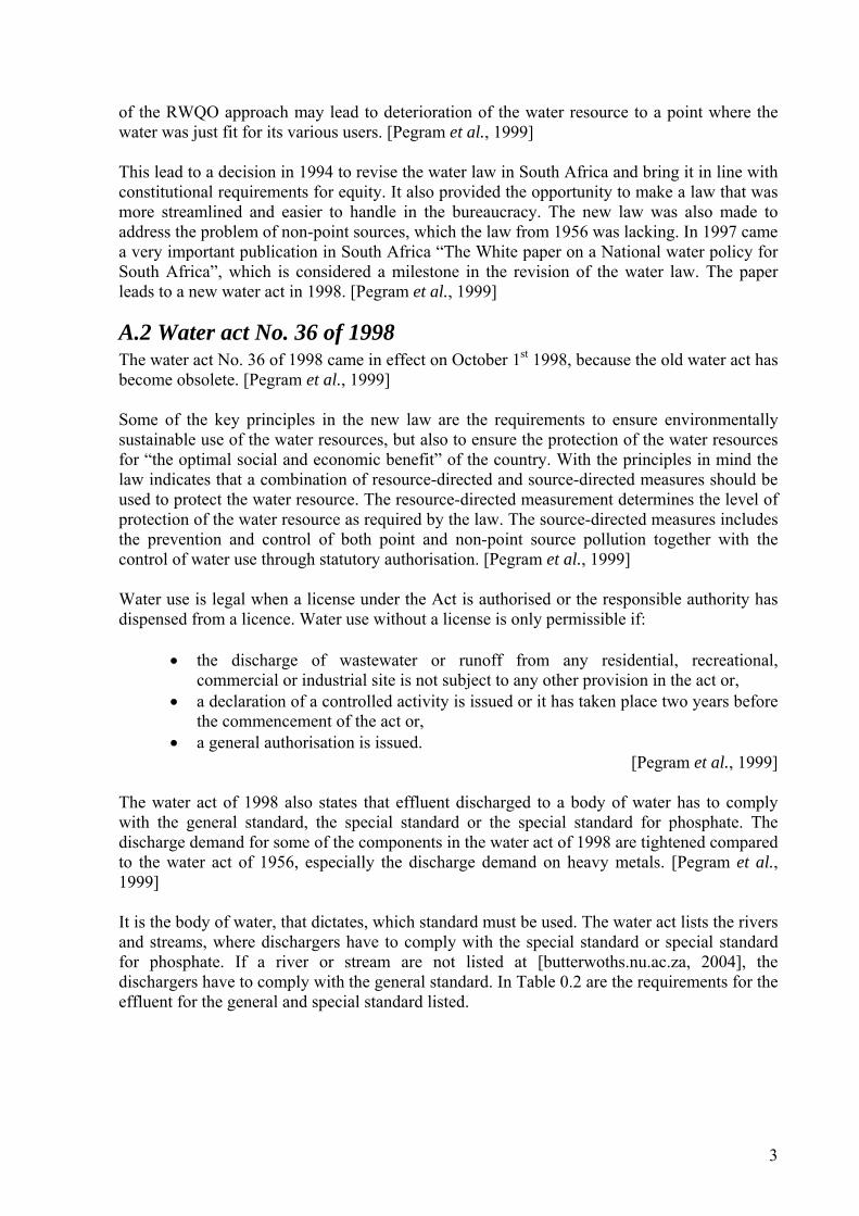
of the RWQO approach may lead to deterioration of the water resource to a point where the water was just fit for its various users. [Pegram et al., 1999] This lead to a decision in 1994 to revise the water law in South Africa and bring it in line with constitutional requirements for equity. It also provided the opportunity to make a law that was more streamlined and easier to handle in the bureaucracy. The new law was also made to address the problem of non-point sources, which the law from 1956 was lacking. In 1997 came a very important publication in South Africa “The White paper on a National water policy for South Africa”, which is considered a milestone in the revision of the water law. The paper leads to a new water act in 1998. [Pegram et al., 1999]

A.2 Water act No. 36 of 1998 The water act No. 36 of 1998 came in effect on October 1st 1998, because the old water act has become obsolete. [Pegram et al., 1999] Some of the key principles in the new law are the requirements to ensure environmentally sustainable use of the water resources, but also to ensure the protection of the water resources for “the optimal social and economic benefit” of the country. With the principles in mind the law indicates that a combination of resource-directed and source-directed measures should be used to protect the water resource. The resource-directed measurement determines the level of protection of the water resource as required by the law. The source-directed measures includes the prevention and control of both point and non-point source pollution together with the control of water use through statutory authorisation. [Pegram et al., 1999] Water use is legal when a license under the Act is authorised or the responsible authority has dispensed from a licence. Water use without a license is only permissible if:

• the discharge of wastewater or runoff from any residential, recreational, commercial or industrial site is not subject to any other provision in the act or,

• a declaration of a controlled activity is issued or it has taken place two years before the commencement of the act or,

• a general authorisation is issued. [Pegram et al., 1999]

The water act of 1998 also states that effluent discharged to a body of water has to comply with the general standard, the special standard or the special standard for phosphate. The discharge demand for some of the components in the water act of 1998 are tightened compared to the water act of 1956, especially the discharge demand on heavy metals. [Pegram et al., 1999] It is the body of water, that dictates, which standard must be used. The water act lists the rivers and streams, where dischargers have to comply with the special standard or special standard for phosphate. If a river or stream are not listed at [butterwoths.nu.ac.za, 2004], the dischargers have to comply with the general standard. In Table 0.2 are the requirements for the effluent for the general and special standard listed.

3

Table 0.2. General and special standards for discharge in terms of the South African water act No. 36 of 1998. The numbers highlighted in bold differ from the standard in the water act No. 54 of 1956. [butterwoths.nu.ac.za, 2004]

Parameter Unit General standard Special standard Colour, odour, taste [-] Nil Nil PH [-] 5,5 – 9,5 5,5 – 7,5 Dissolved Oxygen [%] > 75 >75 Temperature [°C] < 35 < 25 Typical Faecal coliforms [per 100 ml] Nil Nil Chemical Oxygen Demand [mg O2/L] < 75 < 30 Oxygen absorbed [mg O2/L] < 10 < 5 Conductivity [-] < 75 mS/m < 15% Suspended solids [mg SS/L] < 25 <10 Sodium [mg Na/L] < 90 < 50 Soap, oil, grease [mg/L] < 2,5 Nil Residual chlorine [mg Cl/L] < 0,1 Nil Free and saline ammonia [mg N/L] < 10 < 1,0 Nitrate [mg N/L] Not Specified < 1,5 Arsenic [mg As/L] < 0,5 < 0,1 Boron [mg B/L] < 1,0 < 0,5 Chromium – hexavalent [mg Cr/L] < 0,05 1 < Not specified Chromium – total [mg Cr/L] < 0,5 1 < 0,05 Copper [mg Cu/L] < 1,0 1 < 0,02 Phenol [mg/L] < 0,1 < 0,01 Lead [mg Pb/L] < 0,1 1 < 0,1 Ortho phosphate [mg P/L] Not specified 2 < 1,0

Sulphides [mg S/L] < 1,0 < 0,05 Fluorides [mg F/L] < 1,0 < 1,0 Zinc [mg Zn/L] < 5,0 < 0,3 Iron [mg Fe/L] Not specified < 0,3 Manganese [mg Mn/L] < 0,4 < 0,1 Cyanide [mg CN/L] < 0,5 < 0,5 Cadmium [mg Cd/L] < 0,05 1 < 0,05 Mercury [mg Hg/L] < 0,02 1 < 0,02 Selenium [mg Se/L] < 0,05 < 0,05 1: The sum of the selected shall not exceed 1 mg/L 2: Special standard for phosphate: Soluble ortho phosphate < 1,0 mg P/L A factory, which discharges into a sewer pipe running to a municipal WWTP, has a different set of quality limits to observe. The limits are set by the municipal council, where the factory is situated. In Durban, where the WWTP of interest is located, there are three different sets of quality limits for the industry to observe. The limits depend on the size of the WWTP at the end of the sewer pipe and if the discharge is directly to the sea. The discharge quality limits for industries in Durban are compared to the general standard of the water act from 1998 in Table 0.3.

4

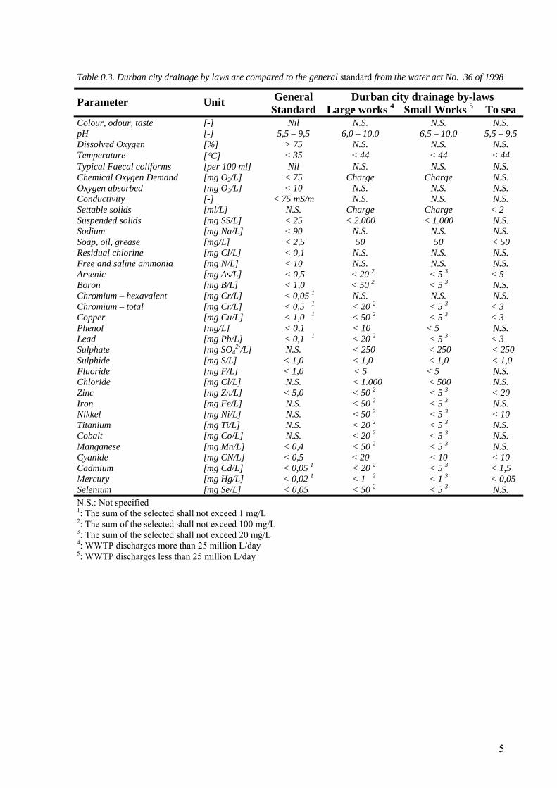
Table 0.3. Durban city drainage by laws are compared to the general standard from the water act No. 36 of 1998

Durban city drainage by-laws Parameter Unit General Standard Large works 4 Small Works 5 To sea

Colour, odour, taste [-] Nil N.S. N.S. N.S. pH [-] 5,5 – 9,5 6,0 – 10,0 6,5 – 10,0 5,5 – 9,5 Dissolved Oxygen [%] > 75 N.S. N.S. N.S. Temperature [°C] < 35 < 44 < 44 < 44 Typical Faecal coliforms [per 100 ml] Nil N.S. N.S. N.S. Chemical Oxygen Demand [mg O2/L] < 75 Charge Charge N.S. Oxygen absorbed [mg O2/L] < 10 N.S. N.S. N.S. Conductivity [-] < 75 mS/m N.S. N.S. N.S. Settable solids [ml/L] N.S. Charge Charge < 2 Suspended solids [mg SS/L] < 25 < 2.000 < 1.000 N.S. Sodium [mg Na/L] < 90 N.S. N.S. N.S. Soap, oil, grease [mg/L] < 2,5 50 50 < 50 Residual chlorine [mg Cl/L] < 0,1 N.S. N.S. N.S. Free and saline ammonia [mg N/L] < 10 N.S. N.S. N.S. Arsenic [mg As/L] < 0,5 < 20 2 < 5 3 < 5 Boron [mg B/L] < 1,0 < 50 2 < 5 3 N.S. Chromium – hexavalent [mg Cr/L] < 0,05 1 N.S. N.S. N.S. Chromium – total [mg Cr/L] < 0,5 1 < 20 2 < 5 3 < 3 Copper [mg Cu/L] < 1,0 1 < 50 2 < 5 3 < 3 Phenol [mg/L] < 0,1 < 10 < 5 N.S. Lead [mg Pb/L] < 0,1 1 < 20 2 < 5 3 < 3 Sulphate [mg SO4

2-/L] N.S. < 250 < 250 < 250 Sulphide [mg S/L] < 1,0 < 1,0 < 1,0 < 1,0 Fluoride [mg F/L] < 1,0 < 5 < 5 N.S. Chloride [mg Cl/L] N.S. < 1.000 < 500 N.S. Zinc [mg Zn/L] < 5,0 < 50 2 < 5 3 < 20 Iron [mg Fe/L] N.S. < 50 2 < 5 3 N.S. Nikkel [mg Ni/L] N.S. < 50 2 < 5 3 < 10 Titanium [mg Ti/L] N.S. < 20 2 < 5 3 N.S. Cobalt [mg Co/L] N.S. < 20 2 < 5 3 N.S. Manganese [mg Mn/L] < 0,4 < 50 2 < 5 3 N.S. Cyanide [mg CN/L] < 0,5 < 20 < 10 < 10 Cadmium [mg Cd/L] < 0,05 1 < 20 2 < 5 3 < 1,5 Mercury [mg Hg/L] < 0,02 1 < 1 2 < 1 3 < 0,05 Selenium [mg Se/L] < 0,05 < 50 2 < 5 3 N.S. N.S.: Not specified 1: The sum of the selected shall not exceed 1 mg/L 2: The sum of the selected shall not exceed 100 mg/L 3: The sum of the selected shall not exceed 20 mg/L 4: WWTP discharges more than 25 million L/day 5: WWTP discharges less than 25 million L/day

5

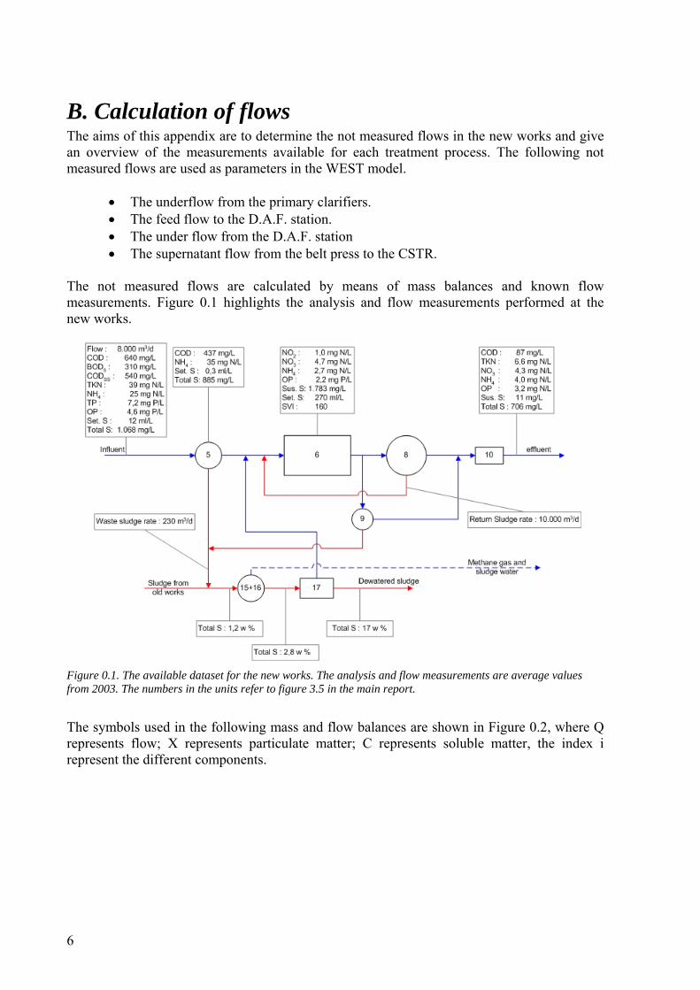
B. Calculation of flows The aims of this appendix are to determine the not measured flows in the new works and give an overview of the measurements available for each treatment process. The following not measured flows are used as parameters in the WEST model.

• The underflow from the primary clarifiers. • The feed flow to the D.A.F. station. • The under flow from the D.A.F. station • The supernatant flow from the belt press to the CSTR.

The not measured flows are calculated by means of mass balances and known flow measurements. Figure 0.1 highlights the analysis and flow measurements performed at the new works.

Figure 0.1. The available dataset for the new works. The analysis and flow measurements are average valuefrom 2003. The numbers in the units refer to figure 3.5 in the main report.

The ances are shown in Figure 0.2, where Q represents flow; X represents particulate matter; C represents soluble matter, the index i

onents.

s

symbols used in the following mass and flow bal

represent the different comp

6

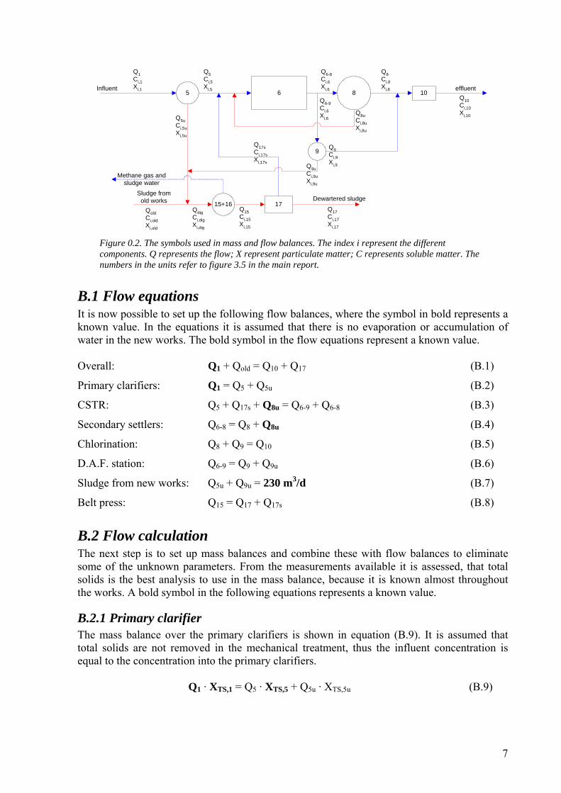
5Influent

6 8

9

10

15+16 17Dewartered sludge

efflu

Q1Ci,1

QCX

Q5uCi,5uXi,5u

Xi,6

Q8Ci,8Xi,8

Q8uCi,8uXi,8u

Q6-9Ci,6Xi,6

Q9uCi,9uXi,9u

Q9Ci,9Xi,9

Q10Ci,1Xi,1

QQ

entXi,1

5

i,5

Q6-8Ci,6

i,5

0

0

Q17sCi,17sXi,17s

Sludge fromold works

QdigQold

Metha

17Ci,17Xi,17

15Ci,15Xi,15

Ci,digXi,dig

Ci,oldXi,old

ne gas andsludge water

re is no evaporation or accumulation of ater in the new works. The bold symbol in the flow equations represent a known value.

verall: Q1 + Qold = Q10 + Q17 (B.1)

Q10 (B.5)

(B.6)

230 m /d (B.7)

17s (B.8)

t up mass ba

e mass balance, because it is known almost throughout e works. A bold symbol in the following equations represents a known value.

B.2.1 Primary clarifier The mass balance over the primary clarifiers is shown in equation (B.9). It is assumed that

tal solids are not removed in the mechanical treatment, thus the influent concentration is

Q1 · XTS,1 = Q5 · XTS,5 + Q5u · XTS,5u (B.9)

Figure 0.2. The symbols used in mass and flow balances. The index i represent the different components. Q represents the flow; X represent particulate matter; C represents soluble matter. The numbers in the units refer to figure 3.5 in the main report.

B.1 Flow equations It is now possible to set up the following flow balances, where the symbol in bold represents a known value. In the equations it is assumed that thew

O

Primary clarifiers: Q1 = Q5 + Q5u (B.2)

CSTR: Q5 + Q17s + Q8u = Q6-9 + Q6-8 (B.3)

Secondary settlers: Q6-8 = Q8 + Q8u (B.4)

Chlorination: Q8 + Q9 =

D.A.F. station: Q6-9 = Q9 + Q9u

3Sludge from new works: Q5u + Q9u =

Q15 = Q17 + QBelt press:

B.2 Flow calculation The next step is to se lances and combine these with flow balances to eliminate some of the unknown parameters. From the measurements available it is assessed, that total solids is the best analysis to use in thth

toequal to the concentration into the primary clarifiers.

7

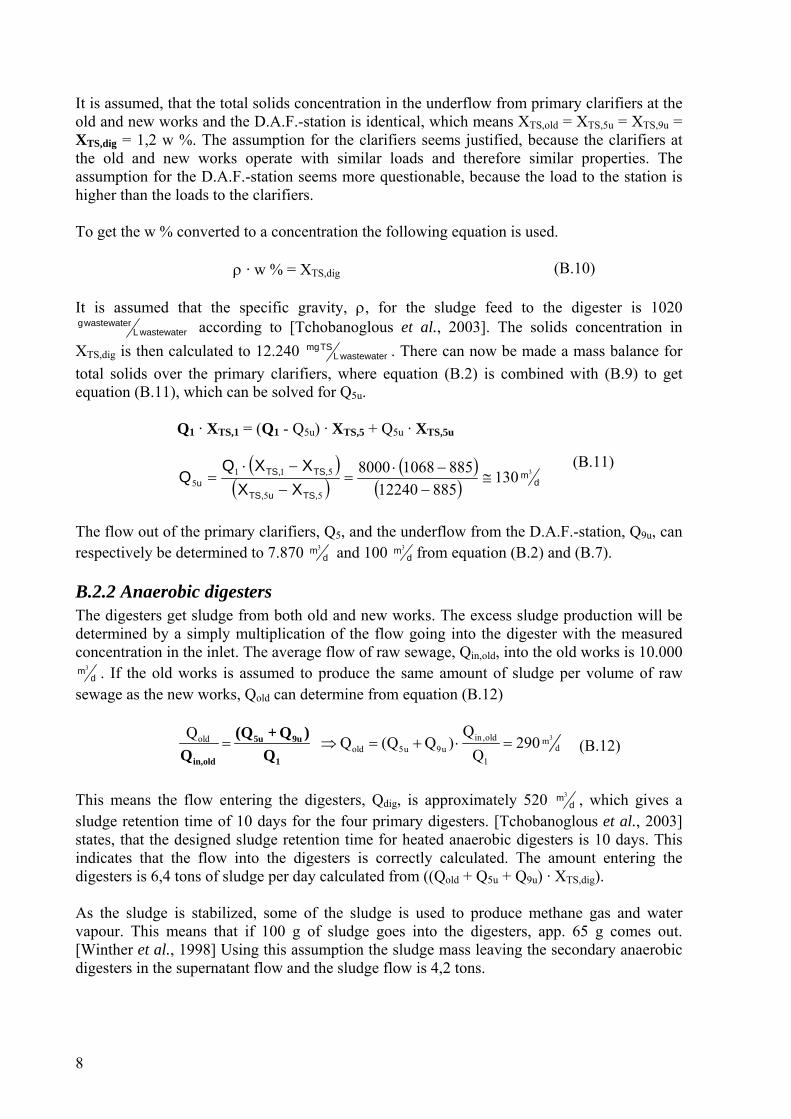
It is assumed, that the total solids concentration in the underflow from primary clarifiers at the

o get the w % converted to a concentration the following equation is used.

ρ · w % = X (B.10)

old and new works and the D.A.F.-station is identical, which means XTS,old = XTS,5u = XTS,9u = XTS,dig = 1,2 w %. The assumption for the clarifiers seems justified, because the clarifiers at the old and new works operate with similar loads and therefore similar properties. The assumption for the D.A.F.-station seems more questionable, because the load to the station is higher than the loads to the clarifiers. T

TS,dig It is assumed that the specific gravity, ρ, for the sludge feed to the digester is 1020

wastewaterLwastewaterg according to [Tchobanoglous et al., 2003]. The solids concentration in

XTS,dig is then calculated to 12.240 wastewaterLTSmg . There can now be made a mass balance for

total solids over the primary clarifiers, where equation (B.2) is combined with (B.9) to get equation (B.11), which can be solved for Q5u.

Q1 · XTS,1 = (Q1 - Q5u) · XTS,5 + Q5u · XTS,5u

( )( )

( )( ) d

m

,TSu,TSu XX

Q 1308851224055

5 ≅−

=−

,TS,TS XXQ 388510688000511 −⋅−⋅=

The flow out of the primary clarifiers, Q

(B.11)

5, and the underflow from the D.A.F.-station, Q9u, can respectively be determined to 7.870 d

m3 and 100 dm3 from equation (B.2) and (B.7).

B.2.2 Anaerobic digesters The digesters get sludge from both old and new works. The excess sludge production will be

ply multiplication of the flow going into the digester with the measured determined by a simconcentration in the inlet. The average flow of raw sewage, Qin,old, into the old works is 10.000

dm3 . If the old works is assumed to produce the same amount of sludge per volume of raw ewage as the new works, Qold can determine from equation (B.12)

s

3in,oldold mdold 5u 9u

1

Q (Q Q ) 290Q

= ⇒ = + ⋅ =5u 9u

in,old 1Q Q (B.12)

This means the flow entering the digesters, Q

QQ (Q + Q )

dig, is approximately 520 dm3 , which gives a

sludge retention time of 10 days for the four primary digesters. [Tchobanoglous et al., 2003] states, that the designed sludge retention time for heated anaerobic digesters is 10 days. This indicates that the flow into the digesters is correctly calculated. The amount entering the

igesters is 6,4 tons of sludge per day calculated from ((Qold + Q5u + Q9u) · XTS,dig). As the sludge is stabilized, some of the sludge is used to produce methane gas and water vapour. This m sters, app. 65 g comes out. [Winther et al., 1998] Using this assumption the sludge mass leaving the secondary anaerobic digesters in the supernatant flow and the sludge flow is 4,2 tons.

d

eans that if 100 g of sludge goes into the dige

8

Because anaerobic digested solids may not settle very well, the supernatant drawn from the eason for poor

settling characteristics can be incomplete digestion in the primary tank, which generates gases causes floating solids. Another reason could be that fine sized solids

he flow entering the belt press, Q15, can now be calculated from the assumed sludge mass

second-stage tank may contain high concentrations of suspended solids. R

in the secondary tank anddo not settle very well. [Tchobanoglous et al., 2003] USPW has not measured the suspended solids concentration in the supernatant. It is however assumed that the total mass of sludge only leaves the digesters in the sludge flow.

B.2.3 Belt Press Tflow, MTS, entering the belt press and the measured sludge concentration, XTS,15:

3TSMQ Q= ⋅ ⇒ =M X md15 15

TS,15

145X

=TS TS,15 (B.13)

is assumed that the w % of TS in the effluent from the belt press is 0,5 [Henze, 2000] and e specific gravity of the effluent is 1010 kg/m3 [Tchobanoglous et al., 2003]. This gives a

oncentration of 5,05 kg TS/m3. The specific gravity of the influent and sludge cake is ssumed to res c 1 et al., 2003], which gives

concentration o /m3. A mass balance c be set up and equation (B ) be i u ( ) to determine the supernatant flow from the belt pres 17s

Q17s · XTS,17s

Itthca pe tively 1020 and 070 kg/m3 [Tchobanoglous

respectively 28,56 kg/mf 3 and 181,9 kg an now.8 can comb ned with eq ation B.14

, Q , from equation (B.15). s

Q15 · XTS,15 = Q17 · XTS,17 + Q17s · XTS,17s (B.14) Q15 · XTS,15 = (Q15 – Q17s ) · XTS,17 +

( )( )

( )( )

3md17s

TS,17s TS,17

6 181,9125

5,05 181,9X X−

=−−

(B.15)

The dew

B.2.4 D.A.F.-station The flow to the D.A.F. station is determined as a fraction of the total flow out of the activated sludge unit. It is assumed that the effluent concentration for the secondary settlers and D.A.F.- station is identical and equal to the effluent concentration from the new works, XSS,8 = XSS,9 = XSS,10 = 11 mg/L. This assumption is justified, because the secondary settlers and D.A.F.-station operate with similar influent concentrations and hydraulic retention times. The concentration of suspended solids for the influent, effluent and underflow from the D.A.F-station is known and equation (B.16) can be combined with equation (B.6) to determine the flow to the D.A.F.-station, Q6-9, equation (B.17).

15 TS,15 TS,17Q X X 145 28,5Q

⋅ − ⋅= =

atered sludge flow, Q17, is estimated to 20 m3/d from equation (B.8.)

9

Q · X = Q · X + Q · X (B.16) 6-9 SS,6 9 SS,9 9u SS,9u Q · X = (Q – Q ) · X + Q · X6-9 SS,6 6-9 9u SS,9 9u SS,9u

( )( )

( )( ) d

m

,SS,SS

,SSu,SSu

XXXXQ

Q 3690111783

1112240100

96

99996 =

−−⋅

=−

−⋅=−

(B.17)

From equation (B.3) the flow to the secondary settlers, Q6-8, is determined to 17.300 d

m3 .

B.3 Flow balance for the new works Flow ra

tes for the new works are shown in Figure 0.3.

Figu nits refers to figure 3.5 in

3re 0.3. The flow rates at the new works. The numbers in the u

the main report. The unit is m /day.

10

C Theory to determine model fractions and parameters The cite reference in this appendix is [Hvitved-Jacobsen, 2002] unless otherwise stated. The appendix lists the theory for the determination of COD fractions and parameters for the CSTR at USPW. The procedure is divided into three experiments based on measurements of Oxygen Uptake Rate (OUR) and Nitrate Uptake Rate (NUR). From the measurements of OUR and NUR eleven model specific COD fractions and parameters are determined from the three experiments:

• Experiment No. 1: Long term measurements of OUR on activated sludge in use. - Lysis and decay rate for heterotrophic biomass, bH

• Experiment No. 2: Long term measurements of OUR with addition of readily biodegradable substrate to raw sewage.

- Yield coefficient for heterotrophic biomass, YH - Maximum growth rate for heterotrophic biomass, µH - Heterotrophic biomass, XH - Slowly biodegradable substrate, XS - Hydrolysis rate constant, kh - Saturation coefficient for SS, KS - Saturation coefficient for particulate COD, KX

• Experiment No. 3: Short term measurements of OUR and NUR on the activated sludge in use.

- Saturation coefficient for oxygen for heterotrophic biomass, KO_H

The fol cific fractions and parameters.

.1 T the model constant, bH

The xponential decrease of the bio H itional decay coefficient. To e adjusted according to the values of the

iel o H ass,

- Saturation coefficient for nitrate for heterotrophic biomass, KNO_H - Reduction factor for denitrification, ηNO

lowing sections introduce, the theory used to determine the eleven model spe

C.1 Experiment No. 1

C .1 heory for determination of plot of the natural logarithm of OUR vs. time visualizes the e

pe, b´ , which refers to the tradmass as a straight line with the sloobtain the model specific parameter, bH, b´H must bd c efficient for heterotrophic biomass, Y , and the fraction of inert particulate biomy

fp, in equation (C.1).

HH

H P

b´b1 Y (1 f )

=− ⋅ −

(C.1)

[Henze et al., 1986] The yield coefficient can be found by the theory described in section 0 and a value of 0,08 g COD/g COD for the fraction of inert particulate biomass is in [Henze et al., 1986] proposed as an acceptable value for all types of wastewater.

11

C.2 Experiment No. 2 A principle pattern of an OUR-curve of measurements on raw incoming sewage with addf readily biodegradable is shown in Figure 0.1. The curve is divided i

ition nto different substrate

ondition. The area above the slowly biodegradable curve, OUR (X ), is a result of the micro the

e

The OUR-curve can be divided into the following substrate condition, where the numbers refer to Figure 0.1.

ited condition. 2. Substrate non-limited condition is just being terminated.

ubstddit

beginning

hydrolysis e

strate is added. The added readily biodegradable substrate ediately growth of the biom er substrate non-limited conditions, where

UR increases, followed by a rapid decrease in OUR (4).

ulate the OUR curve. The original matrix model in [Hvitved-Jacobsen, 2002]

oc Sorganism’s utilization of readily biodegradable substrate and the area below a result ofutilization of slowly biodegradable substrate.

OU

R [m

g O

2/(l⋅h

r)]

1 2 43

SS

X

∆SO,growth

∆SO,maintS

OUR (XS) OURtotal

t = d Time [hr]

Figure 0.1. A principle pattern of an OUR-curve on raw incoming sewage with addition of readily biodegradable substrate. The curve is divided into different substrate condition indicated by thvertically dot-and-dash lines. 1: Substrate non-limited condition, 2: Substrate non-limiting condition is just terminated, 3: Substrate limited condition, 4: Addition of readily biodegradable substrate.

1. Substrate non-lim

3. S rate limited condition. 4. A ion of readily biodegradable substrate.

The figure shows that the original amount of readily biodegradable substrate in the is not limiting for the growth of biomass as the OUR increases (1). This is followed by a sharp

crease in OUR, when the readily biodegradable substrate is depleted (2). After this period dethe readily biodegradable substrate is only available as a result of production fromof slowly biodegradable substrate (3). When the production of readily biodegradable substratby hydrolysis correspond to the required maintenance energy for biomass, i.e. the OUR istabile, readily biodegradable subs

results in an imm ass undO With the above data interpretation of the OUR curve in mind a matrix model can be ormulated to simf

12

is modified to suit the COD fractions needed for the CSTR model. The modification means, that the originally two fractions of hydrolysable substrate are combined to one fraction of slowly biodegradable substrate. The OUR model is shown in Table 0.1.

t ed as OUR ded in the

Table 0.1. The matrix model describes the aerobic utilization of substrate in wastewa er conductmeasurements in a batch reactor. Only one fraction of slowly biodegradable substrate, XS, is inclumodel.

COD fractions Process SS XS XH

- SO Rate

Biomass growth HY1− 1

( )H

HYY1− HSK

SH X

SS

S ⋅⋅µ +

Maintenance energy requirements -1 -1 1 1 Hm Xq ⋅

Hydrolysis of slowly biodegradable substrate -1 1 HKh XkHX

SXX

HXSX

⋅⋅+

1: If SS is not present in sufficient concentration, XH is used for endogenous respiration. qm : Maintenance requirements rate constant [hr-1] The matrix is used as a basis to determine the COD fractions and the parameters either by simple interpretation of the equations in sections 0 and 0, or by fitting the modelled OUR curve to the measured in section 0. The substrate conditions are decisive for which COD-fractions and model-parameters that can be determined from the different part of the OUR-curve. The following sections describes the determination of model constants and COD-fraction from a pragmatically point of view.

hH

ed. The yield constant can be found from equation (C.2), when only condition No. 4 in

C.2.1 T eory for determination of the model constants, YH and µH The yield constant, Y , tells how many g COD biomass produced per g COD totally onsumc

Figure 0.1 is taken into account.

addS

growthSaddSH S

SSY

,

,,

∆

∆−∆= (C.2)

where: ∆SS,add = Amount of added readily biodegradable substrate [mg O2/L] ∆SS,growth = Oxygen uptake for growth [mg O2/L]

can at this stage be described as an exponential

∆SS,growth can in condition No. 4 be found as the area under the curve minus the area corresponding to the oxygen uptake for maintenance energy Under the first part of the experiment, condition No. 1, the biomass undergoes an exponentially increased growth and the OUR

nction, equation (C.3). fu

)exp()()( 0 ttOURtOUR H ∆⋅⋅= µ (C.3)

13

The maximum specific growth rate, µH, is isolated from equation (C.3) and determined in equation (C.4).

( )0

)()(

0ln

tttOURtOUR

H −=µ (C.4)

C.2.2 Theory for determination of the COD fractions, SS, XH and XS

According to the division of the OUR-curve in Figure 0.1 S is calculated fromS equation (C.5). The concentration of SS is given by 1/(1-YH) times the area between the observed CODtotal and the calculated theoretical OUR (XS) from when the measurement starts and to the precipitous drop time (t = d), i.e. where no easily biodegradable substrate is left. OUR (XS) is the OUR used to utilize slowly biodegradable substrate and is a theoretical calculated value. The methods for determining the curve of OUR (XS) are described in annex V.

∫=

=

=

⋅⋅−

=dt

0t SH

S

0tH

dt)S(OURY1

1S

Y (C.5)

∫=

⋅−⋅dt

Stotal dt))X(OUROUR(

ergy of the biomass. The terpretation of this division is shown under (4) in Figure 0.1. With this in mind OUR can be

determined at any time, t, from equation (C.6

−=S 1

1S

SS is determined by integrating the equations graphically. Referring to the matrix model in Table 0.1 the OUR is divided into two parts, an uptake for growth and a corresponding uptake for maintenance requirement enin

).

⎛ ⎞−= + = ⋅ ⋅ + ⋅⎜ ⎟+⎝ ⎠

O,growth O,maint SHH m H

S

dS dS S1 YOUR( t ) q XS

µ (C.6) H Sdt dt Y K

Where qm is the maintenance requirements rate constant, that is determined from equation (C.7).

growthO

maOYY

Hm S

Sq H

H

,

int,1

∆

∆⋅⋅=

−µ (C.7)

es much greater than KS and the monod-expression, S/(KS+SS), is simplified to a unity. The initial heterotrophic biomass at t = 0 is then isolated

and found by equation (C.8).

When readily biodegradable substrate is added, the growth process corresponds to substrate non-limited condition, hence SS becomS

mHYY

tH

OURX

H

H= −

=1

0 (C.8)q+⋅ µ

ecause the OUR is carried out over only app. 24 hours, the duration isn’t sufficient to measure the degradation of slowly biodegradable substrate, XS. Furthermore the degradation

B

14

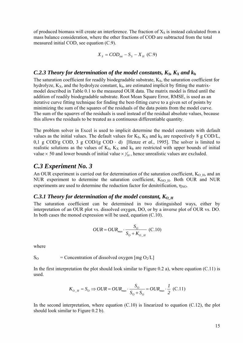
of produced biomass will create an interference. The fraction of XS is instead calculated from a mass balance consideration, where the other fractions of COD are subtracted from the total measured initial COD, see equation (C.9).

HStotS XSCODX −−= (C.9)

C.2.3 Theory for determination of the model constants, KS, KX and kh

The saturation coefficient for readily biodegradable substrate, KS, the saturation coefficient for hydrolyze, KX, and the hydrolyze constant, kh, are estimated implicit by fitting the matrix-model described in Table 0.1 to the measured OUR data. The matrix model is fitted until the addition of readily biodegradable substrate. Root Mean Square Error, RMSE, is used as an

erative curve fitting technique for finding the best-fitting curve to a given set of points by inimizing the sum of the squares of the residuals of the data points from the model curve.

The sum of the squares of the residuals is used instead of the residual absolute values, because this allows the residuals to be treated as a continuous differentiable quantity. The problem solver in Excel is used to implicit determine the model constants with default values as the initial values. The default values for KS, KX and kh are respectively 8 g COD/L, 0,1 g COD/g COD, 3 g COD/(g COD ⋅ d) [Henze et al., 1995]. The solver is limited to realistic solutions as the values of KS, KX and kh are restricted with upper bounds of initial value × 50 and lower bounds of initial value ×

itm

150 , hence unrealistic values are excluded.

C.3 Experiment No. 3 An OUR experiment is carried out for determination of the saturation coefficient, KO_H, and an NUR experim th OUR and NUR experiments a n factor for denitrification, ηNO.

C.3.1 Theory for determination of the model constant, KO_H

ed ways, either by

on (C.10).

ent to determine the saturation coefficient, KNO_H. Bore used to determine the reductio

The saturation coefficient can be determined in two distinguishinterpretation of an OUR plot vs. dissolved oxygen, DO, or by a inverse plot of OUR vs. DO. In both cases the monod expression will be used, equati

= ⋅+

OSmax

O O _ H

OUR OURS K

(C.10)

where

here equation (C.11) is

SO = Concentration of dissolved oxygen [mg O2/L]

In the first interpretation the plot should look similar to Figure 0.2 a), wused.

= ⇒ = ⋅ = ⋅+O

O _ H O maxS

maxO O

1K S OUR OUR OURS S 2

(C.11)

In the second interpretation, where equation (C.10) is linearized to equation (C.12), the plot should look similar to Figure 0.2 b).

15

16

⎛ ⎞ O _ HK1 1 1 1

=1

OUR OU OUR

, where the slope i

⋅ + ⋅ = ⋅ +⎜ ⎟⎝ ⎠

O _ Hmax O max O max

1 KR S S OUR

(C.12)

Equation (C.12) results in a straight line s O _ H

max

KOUR , the intercept with y-axis is

maxOUR1 and the intercept with the x-axis is

−O _ H

1K .

a)

OUR 1 b)

max

O

OURK

max OUR 1

OK1

. O .D1

Figure 0.2. Determination of KO_H by reading a) the monod-curve or b) linear regression of monod-equation.

C.3.2 Theory for determination of the model constant, KNO_H

The saturation coefficient can be determined by reading an NUR vs. concentration of nitrate plot, when a monod equation is used, equation (C.13).

−

−

= ⋅+

3

3

NOmax

NO _ HNO

SNUR NUR

S K (C.13)

where

= Concentration of nitrate [mg N/L] −3NO

S

. The plot is similar to Figure 0.2 a) and the determination is done in the same way

C.3.3 Theory for determination of the model constant, ηNO

The correction factor for denitrification can be calculated from equation (C.14).

OURNUR

NO =η (C.14)

It is here worth to notice, that the unit for both NUR and OUR have to be converted to electron equivalents per volume per time in order to calculate the correction factor. It is easily done, when the following is known [Henze et al., 2002]: 32 g oxygen = 1 mole O2 = 4 electron equivalent. 14 g nitrate-N = 1 mole −NO = 5 electron equivalent. 3

C.4 Check of COD recovery A mass balance of oxygen shows whether the data from the OUR measurements are acceptable. Before and after the experiment a sample was drawn to obtain the initial COD and end COD. A mass balance is constructed, see equation (C.15).

100cov%0

0 ⋅⋅+

==

=

== ∫t

Tt

tTt

COD

dtOURCODeryreCOD (C.15)

where:

= Time [hours] T xperiment [hours]

Dt=T e end of experiment [mg COD/L]

d of experiment [mg

2/L]

recovery/mass balance in the range of 95-105 % indicates that the OUR measurements are r i

t = Time used at the end of the e

OC = Total COD concentration at thCODt=0 = Total COD concentration at the beginning of experiment [mg COD/L]

∫=

=⋅

Tt

tdtOUR

0 = Integral of the OUR vs. time curve between start and en

O

A CODel able [Wentzel et al., 1995].

17

D Sub-models available in the WEST program his appendix gives a description of the sub- available for the primary clarifiers, CSTR nd the secondary settlers in the WEST pro odels governing equations are

with a brief description. The cite reference in this chapter is [WEST models guide,

iers in the WEST program is a point ettler primary clarifier. The other sub-models available are Otterpohl & Freund, Tay and

t described here, because they are similar to the original Takacs sub-model. There also a further sub-model, Lessard Beck available but only with the activated sludge model

e sub-model is not described. The notation in the following equations

ettler. It is not a dynamical sub-model but nly based on mass balances. It is assumed that there are no biological reactions.

To calculate the over- and underflow fluxes a mass balance over the clarifier is solved. The soluble overflow flux is calculated from the flow rates in the inlet, Q1, and overflow, Q5, i.e. soluble readily biodegradable substrate flux, , in the overflow is calculated in equation

T modelsgram. The sub-ma

shown 2004]

D.1 Primary clarifier The selected sub-model to represent the primary clarifsTakacs primary clarifier. There are three extensions of the Takacs sub-model available, but they are noisNo 1 selected, thus threfers to Figure 0.2, if nothing else is written.

D.1.1 The selected sub-model The modelling of a settler by means of a point settler is a large simplification of the actual process. The settler is only a phase separator, and has no real volume. Hence, the sub-model does not take into account the retention time in the so

5,SFJ

(D.1).

S S

5S ,5 S ,1

1

QJ JQ

= ⋅ (D.1.)

f SS in Q1 [g SS/d]

The pa u . the flux of lculated in equation (D.2.)

where J = the mass flux o

SS ,1

rtic late overflow flux is calculated as

inert pa ticulate matter, J , is ca a fraction of the influent flux to the clarifier, e.g

r 5,XI

ns1

where 1,XI

J = the mass flux of X

51,X5,X f

QQ

JJII

⋅⋅= (D.2)

dels ary clarifiers

for the 3 three remaining sub-models are cali ccordingly to equation (D.1)

I in Q1 [g XI/d] fns = the fraction of non-settable solids [-]

D.1.2 The rest of the available sub-moSoluble fractions can not settle and the soluble flux in the overflow from the prim

brated a

18

Otterpohl & Freund primary clarifier The odel of Otterpohl and Freunsub-m d from 1992 for primary clarifiers is based on the

material is reached depending on tion to calculate the particulate matter in the effluent

om primary clarifier is based on an empirical curve, which can also be approximated by the following function, equation (D.3)

assumption that a certain removal efficiency for particulate the hydraulic residence time. The equafr

β+⎟⎟⎠

⎞⎜⎜⎝

⎛⋅α=

2

1

clarifierCOD Q

VlogEff (D.3)

where EffCOD = the percent of COD removed in the primary clarifier [%] VClarifier = the volume of the clarifier [m3].

COD t is removed by the primary

s the hydraulic retention time and the half removal time to in the effluent. The half removal time is the

of the particulate matter. For these ged flow rate, Qaverage, is used. The effluent suspended solids

Alfa, α = an Otterpohl & Freund function constant [-] Beta,β = an Otterpohl & Freund function constant [-] This gives Eff as a percent of the total COD in the influent, thaclarifiers. Tay primary clarifier This clarifier sub-model usecalculate the fraction of particulate matter necessary hydraulic retention time to remove halfcalculations the averaconcentration is calculated in equation (D.4.). A mass balance is solved to find the underflow flux. No biological reactions are taken into account.

A1,average

clarifier

1,i5,i

TQV

1

XX

⋅+

= (D.4.)

= the

ds balance is made. Some ssumptions are made:

he settling velocity, Vsett, of the sludge blanket has been found to be a non-linear function of the solids c In the sub-model the settling flux is due to the gravity settling and also due to the bulk flux, see equation (D.5.). The bulk flux is upward above the feed layer resulting from the overflow rate. Beneath the feed layer the bulk flux is downward resulting from the underflow rate. The gravitational flux is always downwards. The concentration in the bottom layer is identically

where TA half removal time [d] Takacs primary clarifier The settler is modelled with a number of layers around, which a solia

• The incoming solids are distributed immediately homogenous over the feed layer. • Only vertical flow is considered.

T

oncentration.

19

to the sludge the und the under calculated by multiplying the c with the flowHYDRO ECOLO METEO MANAGEMENT INFORMATION SYSTEMS

down

upilayerup

J

xJ

=

concentration in erflow and flow flux isoncentration .

settilayergrav vxJ ⋅=dola wyer vx ⋅

v

ni

⋅=

(D.5)

where rd bulk flux [g/d]

/d]

the CSTR in the WEST program is a fixed volume tank. e variable and pumped volume tanks. There are nine

fore not escribed here.

The three main sub-models use the same matrix to calculate the reaction of the components in

.2.1 The selected sub-model This is an CSTR with a fixed volume. This means that the influent flow rate is the same as the effluent flow rate, Q5 = Q6-8.

The oV iable volu

his is a CSTR, which has one or more weirs and therefore a variable volume. The effluent

Jup, Jdown = the upward and downwaJgrav = the gravitational flux [gvup, vdown = the upward and downward flow velocity [m/d] vsett = the settling velocity [m/d]

D.2 CSTR The selected sub-model to representThe other sub-models available arextensions of the fixed volume model available, but all the sub-model just divide the CSTR at USPW up into smaller compartments. The calculation procedure for several tanks is identically to a fixed volume sub-model with just one tank and the extensions are thered

the CSTR. Where the sub-models differ are in the calculation of the hydraulic retention time, because the effluent flow from the CSTR is calculated differently.

D

D ther sub-models available .2.2ar me tank

Tflow rate depends on the type, width, design and number of weirs, see equation (D.6).

β

− ⎟⎟⎠⎝ A⎞

⎜⎜⎛

⋅α⋅=V

NQ ttancons,TRCSTR86 (D.6.)

ere

width. [-] [-]

3

− VCS

whN = the number of weirs. [-] Alfa, α = depends on the weir type and

depends on the weir design. Beta,β =VCSTR, constant = the volume in the tank below the lowest weir. [m ]

20

Pumped volume tank This is a CSTR, where the volume is controlled with a pump between a maximum and

e tank. Between the two levels the flow rate is constant, Qpump, and

Outlet flow

minimum level of thoutside these levels the outflow equals the inflow, see Table 0.1

Table 0.1. The outlet flow with respect to the inlet flow and volume in the tank.

Volume in tank Inlet flow VCSTR < Vmin Qpump > Q5 Q6-8 = Q5VCSTR < Vmin Qpump ≤ Q5 Q6-8 = Qpump

Vmin ≤ VCSTR < Vmax Q6-8 = Qpump

VCSTR ≥ Vmax Qpump > Q5 Q6-8 = Qpump

VCSTR ≥ Vmax Qpump ≤ Q5 Q6-8 = Q5

Vmin is the minimum volume in the tank [m3] Vmax is the minimum volume in the tank [m3] Qpump is the desired effluent flow rate [m3/d]

D.3 Secondary settler unit he selected sub-model to represent the secondary settler in the WEST program is a Takacs

settler. The other sub-models available are point settler, Marsili Libelli, Otterpohl & Freund and extensions of the Takacs sub-model. The equations in the secondary point settler are identically to the primary point settler, which is described above. The extension in the Takacs sub-model is not described.

D.3.1 The selected sub-model The Takacs sub-model for the primary clarifier and secondary settler uses the same equations, therefore will the sub-model only be briefly described, see section 0. The determination of the velocity of up- and downward flow used in equation (D.5) is shown in equation (D.6).

T

AQ

v

AQ

v

u8down

8up

=

=(D.6)

The calculation of the settling velocity depends on the concentration of particulate matter and below a minimum concentration, the settling velocity is 0. The calculation for the minimum concentration, Xmin, is shown in equation (D.7).

TSSCODFQ

JfX

86

6,solidsnsmin ⋅

⋅=−

(D.7)

where Jsolids,6 = the flux of solids into the secondary settler [g/d]

TSSCODF = the fraction of TSS

COD When the concentration of the particles is above the minimum concentration the settling velocity can be calculated from equation (D.8).

21

minilayerJ

Xr0

Xr0sett

XXXevevv jPjH

⋅=⋅−⋅= ⋅⋅

(D.8)

where v0 = the maximum theoretical settling velocity [m/d] rH = the settling parameter for hindered settling [m3/g] rP = the settling parameter for low concentrations [m3/g]

D.3.2 The other sub-models available Marsili Libelli The settling process exists of two sub-processes, thickening and clarification, of which the first is the most important one. A clarification failure is always the result of a thickening failure. The sub-model is a dynamic presentation for the transfer and accumulation of sludge mass in the secondary clarifier based on the theory of hindered settling without the use of layers. The total downward mass transfer, F, is calculated from a gravitational component, Fg, and a bulk flux component, Fb. (F = Fg + Fb) Otterpohl & Freund Otterpohl & Freund use two components, micro- and macro-flocs, in modelling the sedimentation behaviour. The sub-model divides the settler in 10 layers. The volume of the layers must be at least one order of magnitude larger than the flow rate in one time interval. For each layer a mass balance is formed. The change of mass depends on the bulk flux and the settling flux (gravitational flux), see equation (D.9).

micromicro,ilayermicro,grav

macromacro,ilayermacro,grav

downmicro,ilayermicro,down

downmacro,ilayermacro,down

upmicro,ilayermicro,up

upmacro,ilayermacro,up

vxJ

vxJ

vxJ

vxJ

vxJ

vxJ

⋅=

⋅=

⋅=

⋅=

⋅=

⋅=

(D.9)

22

Table of contents for annexes I Sludge and hydraulic retention time in the CSTR...........1 II Rainfall in the Umgeni area ...............................................2 III General composition of domestic sewage..........................3 IV Threshold concentration for heavy metals .......................4 V Calculation of slowly biodegradable substrate curve ......5 VI Interference concentration for the nitrate probe.............6 VII Model parameters for the CSTR unit ...............................7 VIII Characteristic of sewage sludge.........................................8 IX Utilization of sludge on farm land.....................................9 X Restrictions and recommendations for sludge. ..............10

Table of contents for CD-ROM annexes 1. Chemical and physical analysis from USPW 2. Flow data from USPW from 1999 to 2004 3. Calculation of COD fractions and parameters from each

individual experiment 4. Summary of the COD fractions and parameters 5. Input file for dynamic calibration 6. Optimization of the WEST model with 5 scenarios 7. The RMSE values for the calibration and validation 8. Rainfall in the Umgeni area

2

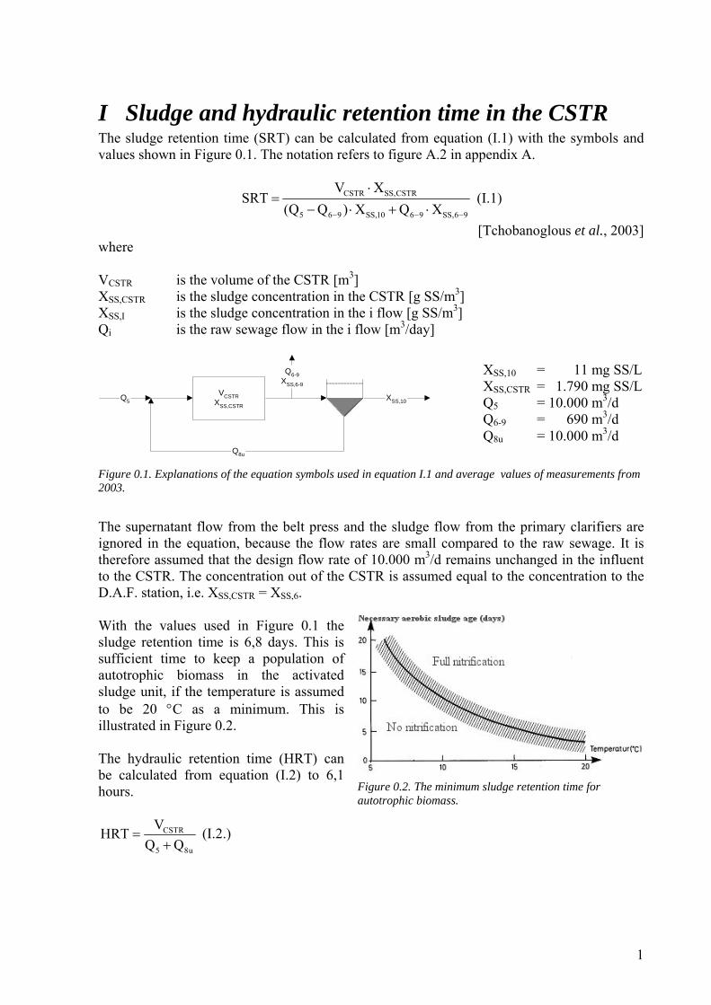
I Sludge and hydraulic retention time in the CSTR The sludge retention time (SRT) can be calculated from equation (I.1) with the symbols and values shown in Figure 0.1. The notation refers to figure A.2 in appendix A.

CSTR SS,CSTR

5 6 9 SS,10 6 9 SS,6 9

V XSRT

(Q Q ) X Q X− − −

⋅

VCSTRXSS,CSTR

Q8u

XSS,10

Q6-9XSS,6-9

Q5

=− ⋅ + ⋅

[Tchobanoglous et al., 2003]

CSTR SS,I m3]

Qi is the raw sewage flow in the i flow [m3/day]

igure 0.1. Explanations of the equation symbols used in equation I.1 and average values of measurements from 003.

the CSTR is assumed equal to the concentration to the

nimum. This is

ulated from equation (I.2) to 6,1 h

(I.1)

where VCSTR is the volume of the CSTR [m ]

/m3 3

XSS, is the sludge concentration in the CSTR [g SSX is the sludge concentration in the i flow [g SS/

]

F2

The supernatant flow from the belt press and the sludge flow from the primary clarifiers are ignored in the equation, because the flow rates are small compared to the raw sewage. It is therefore assumed that the design flow rate of 10.000 m3/d remains unchanged in the influent o the CSTR. The concentration out oft

D.A.F. station, i.e. XSS,CSTR = XSS,6. With the values used in Figure 0.1 the sludge retention time is 6,8 days. This is sufficient time to keep a population of autotrophic biomass in the activated sludge unit, if the temperature is assumed o be 20 °C as a mit

illustrated in Figure 0.2. The hydraulic retention time (HRT) can

e calcbours.

CSTR

5 8

VHRTQ Q

=+ u

(I.2.)

Figure 0.2. The minimum sludge retention time for autotrophic biomass.

XSS,10 = 11 mg SS/L XSS,CSTR = 1.790 mg SS/L Q5 = 10.000 m3/d Q6-9 = 690 m3/d Q = 10.000 m3/d 8u

1

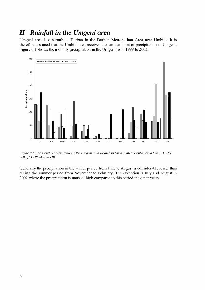
II Rainfall in the Umgeni area Umgeni area is a suburb to Durban in the Durban Metropolitan Area near Umbilo. It is therefore assumed that the Umbilo area receives the same amount of precipitation as Umgeni. Figure 0.1 shows the monthly precipitation in the Umgeni from 1999 to 2003.

0

50

100

150

200

250

300

JAN FEB MAR APR MAY JUN JUL AUG SEP OCT NOV DEC

Prec

ipita

tion

[mm

]

1999 2000 2001 2002 2003

Figure 0.1. The monthly precipitation in the Umgeni area located in Durban Metropolitan Area from 1999 to 2003.[CD-ROM annex 8]

Generally the precipitation in the winter period from June to August is considerable lower than during the summer period from November to February. The exception is July and August in 2002 where the precipitation is unusual high compared to this period the other years.

2

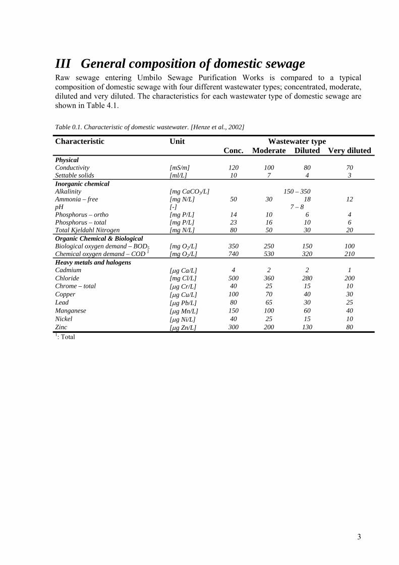
III General composition of domestic sewage Raw sewage entering Umbilo Sewage Purification Works is compared to a typical composition of domestic sewage with four different wastewater types; concentrated, moderate, diluted and very diluted. The characteristics for each wastewater type of domestic sewage are shown in Table 4.1. Table 0.1. Characteristic of domestic wastewater. [Henze et al., 2002]

Wastewater type Characteristic Unit Conc. Moderate Diluted Very diluted

Physical Conductivity [mS/m] 120 100 80 70 Settable solids [ml/L] 10 7 4 3 Inorganic chemical Alkalinity [mg CaCO3/L] 150 – 350 Ammonia – free [mg N/L] 50 30 18 12 pH [-] 7 – 8 Phosphorus – ortho [mg P/L] 14 10 6 4 Phosphorus – total [mg P/L] 23 16 10 6 Total Kjeldahl Nitrogen [mg N/L] 80 50 30 20 Organic Chemical & Biological Biological oxygen demand – BOD5 [mg O2/L] 350 250 150 100 Chemical oxygen demand – COD 1 [mg O2/L] 740 530 320 210 Heavy metals and halogens Cadmium [µg Ca/L] 4 2 2 1 Chloride [mg Cl/L] 500 360 280 200 Chrome – total [µg Cr/L] 40 25 15 10 Copper [µg Cu/L] 100 70 40 30 Lead [µg Pb/L] 80 65 30 25 Manganese [µg Mn/L] 150 100 60 40 Nickel [µg Ni/L] 40 25 15 10 Zinc [µg Zn/L] 300 200 130 80 1: Total

3

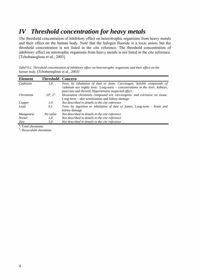
IV Threshold concentration for heavy metals The threshold concentration of inhibitory effect on heterotrophic organisms from heavy metals and their effect on the human body. Note that the halogen fluoride is a toxic anion, but the threshold concentration is not listed in the cite reference. The threshold concentration of inhibitory effect on autotrophic organisms from heavy metals is not listed in the cite reference. [Tchobanoglous et al., 2003] Tabel 0.1. Threshold concentration of inhibitory effect on heterotrophic organisms and their effect on the human body. [Tchobanoglous et al., 2003]

Element Threshold Concern Cadmium 1,0 Toxic by inhalation of dust or fume. Carcinogen. Soluble compounds of

cadmium are highly toxic. Long-term – concentrations in the liver, kidneys, pancreas and thyroid. Hypertension suspected effect.

Chromium 10a, 1b Hexavalent chromium compound are carcinogenic and corrosive on tissue. Long-term – skin sensitization and kidney damage

Copper 1,0 Not described in details in the cite reference Lead 0,1 Toxic by ingestion or inhalation of dust or fumes. Long-term – brain and

kidney damage Manganese No value Not described in details in the cite reference Nickel 1,0 Not described in details in the cite reference Zinc 1,0 Not described in details in the cite reference a: Total chromium b: Hexavalent chromium

4

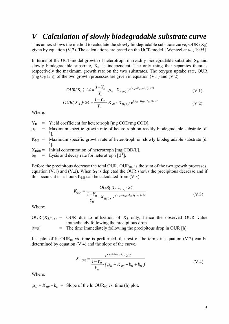
V Calculation of slowly biodegradable substrate curve This annex shows the method to calculate the slowly biodegradable substrate curve, OUR (XS) given by equation (V.2). The calculations are based on the UCT-model. [Wentzel et al., 1995] In terms of the UCT-model growth of heterotroph on readily biodegradable substrate, SS, and slowly biodegradable substrate, XS, is independent. The only thing that separates them is respectively the maximum growth rate on the two substrates. The oxygen uptake rate, OUR (mg O2/L/h), of the two growth processes are given in equation (V.1) and (V.2).

+ − ⋅−

⋅ = ⋅ ⋅ ⋅ H MP H( K b ) t / 2HS H H ( 0 )

H

1 YOUR( S ) 24 X eY

µµ 4 (V.1)

+ − ⋅−⋅ = ⋅ ⋅ ⋅ H MP H( K b ) t / 2H

S MP H ( 0 )H

1 YOUR( X ) 24 K X eY

µ 4

slowly biodegradable substrate [d-

D/L]. -1

ows the precipitous decrease and if is occurs at t = s hours KMP can be calculated from (V.3)

(V.2)

Where: YH = Yield coefficient for heterotroph [mg COD/mg COD]. µH = Maximum specific growth rate of heterotroph on readily biodegradable substrate [d

]. -

1

KMP = Maximum specific growth rate of heterotroph on 1].

concentration of heterotroph [mg COXH(0) = InitialbH = Lysis and decay rate for heterotroph [d ]. Before the precipitous decrease the total OUR, OUR(t), is the sum of the two growth processes, quation (V.1) and (V.2). When Se

thS is depleted the OUR sh

=

+ − ⋅ =

⋅=

−⋅ ⋅ H MP H

S ( t s )MP

( K b ) ( t s ) / 24HH ( 0 )

H

OUR( X ) 24K 1 Y X e

Yµ

(V.3)

XS)(t=s) R value

the terms in equation (V.2) can be etermined by equation (V.4) and the slope of the curve.

Where:

OUR ( = OUR due to utilization of XS only, hence the observed OUimmediately following the precipitous drop.

(t=s) = The time immediately following the precipitous drop in OUR [h]. f a plot of ln OURI

d(t) vs. time is performed, the rest of

− ⋅

=−

⋅ + − +H ( 0 )

HH MP H H

1 Y ( K b bµ

( y int ercept )

H

e 24X)

Y

(V.4)

Where:

+ −H MP HK bµ = Slope of the ln OUR(t) vs. time (h) plot.

5

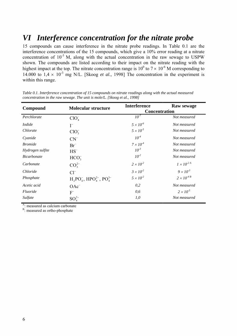
VI Interference concentration for the nitrate probe 15 compounds can cause interference in the nitrate probe readings. In Table 0.1 are the interference concentrations of the 15 compounds, which give a 10% error reading at a nitrate concentration of 10-3 M, along with the actual concentration in the raw sewage to USPW shown. The compounds are listed according to their impact on the nitrate reading with the highest impact at the top. The nitrate concentration range is 100 to 7 × 10-6 M corresponding to 14.000 to 1,4 × 10-3 mg N/L. [Skoog et al., 1998] The concentration in the experiment is within this range. Table 0.1. Interference concentration of 15 compounds on nitrate readings along with the actual measured concentration in the raw sewage. The unit is mole/L. [Skoog et al., 1998]

Interference Raw sewage Compound Molecular structure Concentration

Perchlorate 4ClO− 10-7 Not measured

Iodide I− 5 × 105 -5

-6 Not measured Chlorate

3ClO− × 10 Not measured

Cyanide CN− 10-4 Not measured Bromide Br− 7 -4

N ured

3 -2 -3

− 5

cid

× 10 Not measured Hydrogen sulfite HS− 10-3 Not measured Bicarbonate

3HCO− 10-2 ot meas

Carbonate 23CO − 2 × 10-2 1 × 10-2 A

Chloride

Cl− × 10 9 × 10Phosphate 2 3

2 4 4 4H PO , HPO , PO− − × 10-2 2 × 10-4 B

Acetic a OAc− 0,2 Not measured Fluoride F− 0,6 2 × 10-5

S 1,0 Not measured

: measured as calcium carbonate

ulfate 24SO −

A

B: measured as ortho-phosphate

6

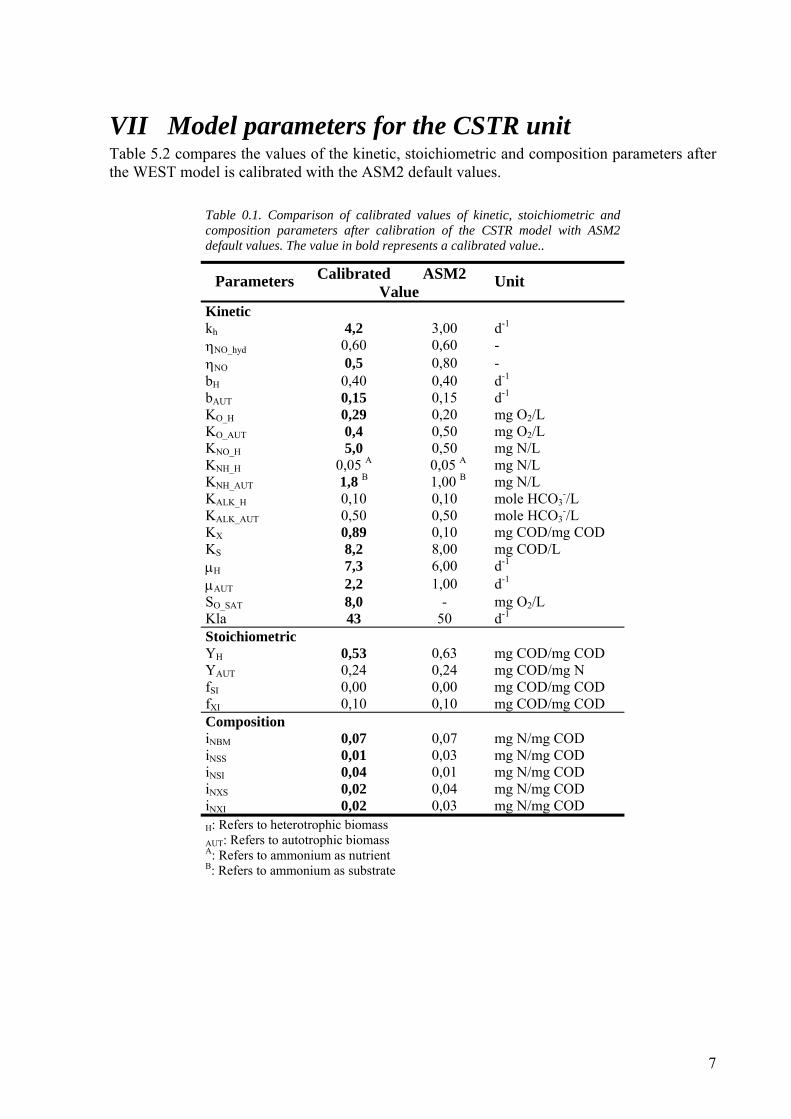
VII Model parameters for the CSTR unit Table 5.2 compares the values of the kinetic, stoichiometric and composition parameters after the WEST model is calibrated with the ASM2 default values.

Table 0.1. Comparison of calibrated values of kinetic, stoichiometric and composition parameters after calibration of the CSTR model with ASM2 default values. The value in bold represents a calibrated value..

Calibrated ASM2 Parameters Value

Unit

Kinetic kh 4,2 3,00 d-1

ηNO_hyd 0,60 0,60 - ηNO 0,5 0,80 - bH 0,40 0,40 d-1

bAUT 0,15 0,15 d-1

KO_H 0,29 0,20 mg O2/L KO_AUT 0,4 0,50 mg O2/L KNO_H 5,0 0,50 mg N/L KNH_H 0,05 A 0,05 A mg N/L KNH_AUT 1,8 B 1,00 B mg N/L KALK_H 0,10 0,10 mole HCO3

-/L KALK_AUT 0,50 0,50 mole HCO3

-/L KX 0,89 0,10 mg COD/mg COD KS 8,2 8,00 mg COD/L µΗ 7,3 6,00 d-1

µΑUT 2,2 1,00 d-1

SO_SAT 8,0 - mg O2/L Kla 43 50 d-1

Stoichiometric YH 0,53 0,63 mg COD/mg COD YAUT 0,24 0,24 mg COD/mg N fSI 0,00 0,00 mg COD/mg COD fXI 0,10 0,10 mg COD/mg COD Composition iNBM 0,07 0,07 mg N/mg COD iNSS 0,01 0,03 mg N/mg COD iNSI 0,04 0,01 mg N/mg COD iNXS 0,02 0,04 mg N/mg COD iNXI 0,02 0,03 mg N/mg COD H: Refers to heterotrophic biomass AUT: Refers to autotrophic biomass A: Refers to ammonium as nutrient B: Refers to ammonium as substrate

7

VIII Characteristic of sewage sludge Table 0.1 divides the sewage sludge into four types of sewage sludge according to how stable the sludge is, where D is most stable and A the least. Table 0.1 The sludge is divided into four types with characteristic properties according to treatment process for the sludge.

Type of sewage sludge

Origin/treatment (Examples)

Characteristic – Quality of sewage sludge

Type A sludge

Raw sludge Cold digested sludge Septic tank sludge Oxidation pond sludge

Usually unstable and can cause odour nuisances and fly-breeding Contains pathogenic organisms Variable metal and inorganic content

Type B sludge

Anaerobic digested sludge (heated digester) Surplus activated sludge Humus tank sludge

Fully or partially stabilised – should not cause significant odour nuisances or fly-breeding Contains pathogenic organisms Variable metal and inorganic content

Type C sludge

Pasteurised sludge Heat-treated sludge Lime-stabilised sludge Composted sludge Irradiated sludge

Has to be certified otherwise type B sludge Stabilised – should not cause odour nuisances or fly-breeding Contains no salmonella organism per 10 g dry sludge Contains maximum 1.000 faecal coliform per 10 g dry sludge Variable metal and inorganic content

Type D sludge

Pasteurised sludge Heat-treated sludge Lime-stabilised sludge Composted sludge Irradiated sludge

Has to certified and comply with same pathogenic content as type C sludge Maximum metal and inorganic content in mg per kg dry sludge: Cadmium 15,7 Cobalt 100 Chromium (Cr3+) 1.750 Copper 50,5 Mercury 10 Molybdenum 25 Nickel 200 Lead 50,5 Zinc 353,5 Arsenic 15 Selenium 15 Boron 80 Flouride 400 User must be informed about moisture and N, P, K content User must be warned that not more than 8 tons dry sludge per hectare may be applied and the pH of the soil should preferable be higher than 6,5

8

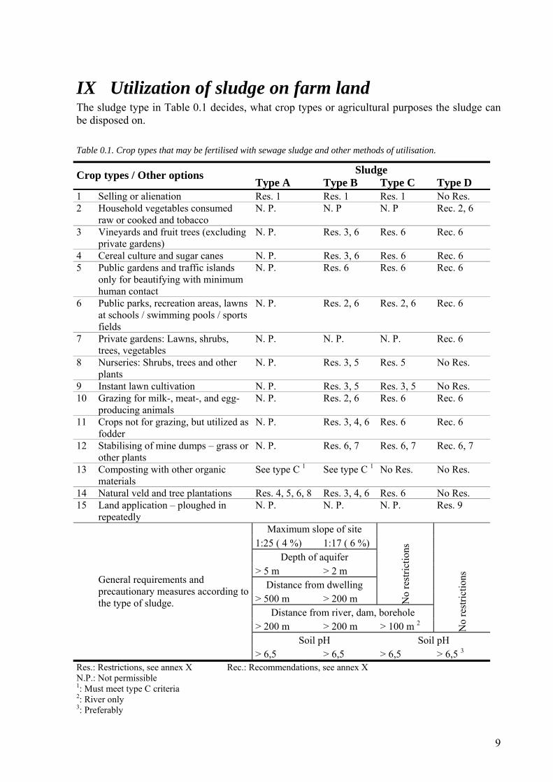
IX Utilization of sludge on farm land The sludge type in Table 0.1 decides, what crop types or agricultural purposes the sludge can be disposed on. Table 0.1. Crop types that may be fertilised with sewage sludge and other methods of utilisation.

Sludge Crop types / Other options Type A Type B Type C Type D

1 Selling or alienation Res. 1 Res. 1 Res. 1 No Res. 2 Household vegetables consumed

raw or cooked and tobacco N. P. N. P N. P Rec. 2, 6

3 Vineyards and fruit trees (excluding private gardens)

N. P. Res. 3, 6 Res. 6 Rec. 6

4 Cereal culture and sugar canes N. P. Res. 3, 6 Res. 6 Rec. 6 5 Public gardens and traffic islands

only for beautifying with minimum human contact

N. P. Res. 6 Res. 6 Rec. 6

6 Public parks, recreation areas, lawns at schools / swimming pools / sports fields

N. P. Res. 2, 6 Res. 2, 6 Rec. 6

7 Private gardens: Lawns, shrubs, trees, vegetables

N. P. N. P. N. P. Rec. 6

8 Nurseries: Shrubs, trees and other plants

N. P. Res. 3, 5 Res. 5 No Res.

9 Instant lawn cultivation N. P. Res. 3, 5 Res. 3, 5 No Res. 10 Grazing for milk-, meat-, and egg-

producing animals N. P. Res. 2, 6 Res. 6 Rec. 6

11 Crops not for grazing, but utilized as fodder

N. P. Res. 3, 4, 6 Res. 6 Rec. 6

12 Stabilising of mine dumps – grass or other plants

N. P. Res. 6, 7 Res. 6, 7 Rec. 6, 7

13 Composting with other organic materials

See type C 1 See type C 1 No Res. No Res.

14 Natural veld and tree plantations Res. 4, 5, 6, 8 Res. 3, 4, 6 Res. 6 No Res. 15 Land application – ploughed in

repeatedly N. P. N. P. N. P. Res. 9

Maximum slope of site 1:25 ( 4 %) 1:17 ( 6 %)

Depth of aquifer > 5 m > 2 m

Distance from dwelling > 500 m > 200 m N

o re

stric

tions

Distance from river, dam, borehole > 200 m > 200 m > 100 m 2 N

o re

stric

tions

Soil pH Soil pH

General requirements and precautionary measures according to the type of sludge.

> 6,5 > 6,5 > 6,5 > 6,5 3

Res.: Restrictions, see annex X Rec.: Recommendations, see annex X N.P.: Not permissible 1: Must meet type C criteria 2: River only 3: Preferably

9

X Restrictions and recommendations for sludge. Annex IX listed the restrictions or recommendations numbers used, when sludge is disposed for agricultural purposes. The restriction and recommendation number is described in Table 0.1. Table 0.1. Restrictions or Recommendations referred to in annex IX

Restrictions / Recommendations 1 Only as per contract. 2 Application only during planting. 3 Application only with planting and during the period subsequent to harvesting and prior to the

next growing season in order to minimize sewage sludge coming into contact with crops to be harvested.

4 Application permissible; only if area is fenced to keep out unauthorised persons as well as milk-, meat-, and egg- producing animals.

5 No subsequent selling or alienation of sludge or any mixture containing such sludge is allowed by the user.

6 All sludge must be mixed or covered with soil when ever possible. 7 Soil pH and slope requirements could be relaxed on condition that no contaminated runoff and

seepage water will pollute any surface or underground water. 8 Application of excessive quantities of sewage sludge to land causes that site to be unfit for any

other purpose during such operation and for a minimum period of two years after termination thereof. (Waste disposal site, see 9) No nuisance or any other condition poising a potential health hazard or which may cause pollution of any water source will be tolerated on such site

9 Disposal of sludge and the co-disposal of sludge with domestic waste and other waste on disposal sites must comply with the following:

− Permit requirements in terms of the Environmental Conservation Act, Act 73 of 1989 − “Minimum Requirements for Waste Disposal by Landfill”, a Department of Water

Affairs and Forestry document.

10

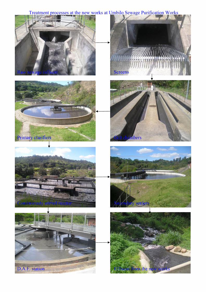
Treatment processes at the new works at Umbilo Sewage Purification Works

Raw sewage influent Screens

Primary clarifiers Grit chambers

Continuously stirred reactor Secondary settlers

D.A.F. station Effluent from the new works