Embed Size (px)
Citation preview
General rights Copyright and moral rights for the publications made accessible in the public portal are retained by the authors and/or other copyright owners and it is a condition of accessing publications that users recognise and abide by the legal requirements associated with these rights.
Users may download and print one copy of any publication from the public portal for the purpose of private study or research.
You may not further distribute the material or use it for any profit-making activity or commercial gain
You may freely distribute the URL identifying the publication in the public portal If you believe that this document breaches copyright please contact us providing details, and we will remove access to the work immediately and investigate your claim.
Downloaded from orbit.dtu.dk on: May 24, 2020
Modelling of wind power plant controller, wind speed time series, aggregation andsample results
Hansen, Anca Daniela; Altin, Müfit; Cutululis, Nicolaos Antonio
Publication date:2015
Document VersionPublisher's PDF, also known as Version of record
Link back to DTU Orbit
Citation (APA):Hansen, A. D., Altin, M., & Cutululis, N. A. (2015). Modelling of wind power plant controller, wind speed timeseries, aggregation and sample results. DTU Wind Energy. DTU Wind Energy E, No. 0080
DTU
Vin
dene
rgi
E R
appo
rt 2
015
Modelling of wind power plant controller, wind speed time series, aggregation and sample results
Anca D. Hansen, Müfit Altin, Nicolaos A. Cutululis
DTU Wind Energy E-0080
January 2015

Forfatter(e): Anca D. Hansen, Müfit Altin, Nicolaos A. Cutululis
Titel: Modelling of wind power plant controller, wind speed time series,
aggregation and sample results Institut: DTU Wind Energy
2015
Resume (mask. 2000 char.):
This report describes the modelling of a wind power plant (WPP) including its
controller. Several ancillary services like inertial response (IR), power
oscillation damping (POD) and synchronising power (SP) are implemented.
The focus in this document is on the performance of the WPP output and not
the impact of the WPP on the power system. By means of simulation tests,
the capability of the implemented wind power plant model to deliver ancillary
services is investigated.
ISBN nr. 978-87-93278-25-7
Kontrakt nr.:
[Tekst]
Projektnr.:
[Tekst]
Sponsorship:
PSO
Forside:
[Tekst]
Danmarks Tekniske Universitet DTU Vindenergi Nils Koppels Allé Bygning 403 2800 Kgs. Lyngby Telefon www.vindenergi.dtu.dk
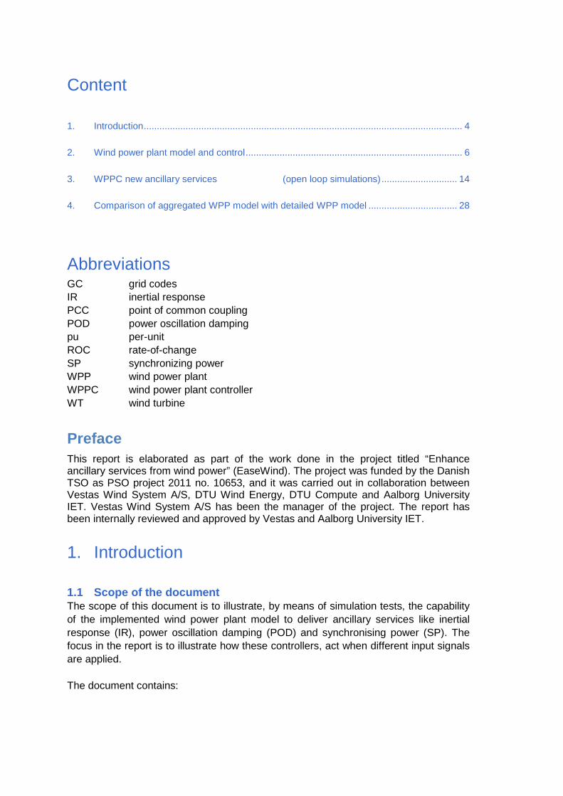
Content
1. Introduction .......................................................................................................................... 4
2. Wind power plant model and control ................................................................................... 6
3. WPPC new ancillary services (open loop simulations) ............................. 14
4. Comparison of aggregated WPP model with detailed WPP model .................................. 28
Abbreviations GC grid codes IR inertial response PCC point of common coupling POD power oscillation damping pu per-unit ROC rate-of-change SP synchronizing power WPP wind power plant WPPC wind power plant controller WT wind turbine
Preface This report is elaborated as part of the work done in the project titled “Enhance ancillary services from wind power” (EaseWind). The project was funded by the Danish TSO as PSO project 2011 no. 10653, and it was carried out in collaboration between Vestas Wind System A/S, DTU Wind Energy, DTU Compute and Aalborg University IET. Vestas Wind System A/S has been the manager of the project. The report has been internally reviewed and approved by Vestas and Aalborg University IET.
1. Introduction
1.1 Scope of the document The scope of this document is to illustrate, by means of simulation tests, the capability of the implemented wind power plant model to deliver ancillary services like inertial response (IR), power oscillation damping (POD) and synchronising power (SP). The focus in the report is to illustrate how these controllers, act when different input signals are applied. The document contains:
• Modelling of the wind power plant controller (WPPC) 1 • Implementation of the WPPC in PowerFactory • Simulation of the control features required today by grid codes (GC) [1] and
future proposed ancillary services • Available power estimation • Generation of wind speed time series • Description of aggregation method • Comparison of detailed wind power plant (WPP) model with aggregated WPP
model through simulations.
1.2 References [1] M. Tsili and S. Papathanassiou, “A review of grid code technical requirements for
wind farms”. IET Renewable Power Generation, 2009, 3, (3), pp. 308-332. [2] A. D. Hansen, I.D. Margaris, “Type IV wind turbine model”, DTU Wind Energy report, 2013. [3] P. Mahat,”Power system Model for New ancillary services”. Report Ålborg University, 2013 [4] Tarnowski, G. C., “Coordinated frequency control of wind turbines in power systems
with high wind power penetration”. Industrial PhD thesis, DTU. Denmark 2012. Available online.
[5] Adamczyk, A., “Damping of Low Frequency Power System Oscillations with Wind Power Plants”, PhD Thesis, Aalborg University, Aalborg, Denmark, 2012.
[6] Kundur, P. “Power System Stability and Control”, New York, USA: McGraw- Hill, Inc., 1994. 1776p. ISBN: 0-07-035958-X.
[7] Hansen, A.D.; Sørensen, P.; Iov,F.; Blaabjerg, F., Centralised power control of wind farm with doubly-fed induction generators, Renewable Energy, vol 31 (2006), 935- 951.
[8] P. Sørensen, et al, “Power Fluctuations from Large Wind Farms”, Risø-R- 1711(EN), 2009
[9] Sørensen, P., Hansen, A. D. & Rosas, P. A. C. Wind models for simulation of power fluctuations from wind farms. Journal of wind engineering and industrial aerodynamics 1381–1402 (2002). doi:10.1016/S0167-6105(02)00260-X
[10] P. Sørensen,, N.A. Cutululis, A. Vigueras-Rodriguez, L.E. Jensen, J. Hjerrild, M.H. Donovan, H. Madsen. Power fluctuations from large wind farms. IEEE Trans. Power Systems (2007) 22, 958-965
1 WPP and WPPC are modelled in continuous time domain. The performance assessment of s-domain control versus
z-domain control is out of the scope of this report.
5
2. Wind power plant model and control
The WPP consists of a number of wind turbines connected through a substation transformer to the plant’s point of common coupling (PCC), a WPPC, and measurement devices for voltage, frequency, current, power at PCC.
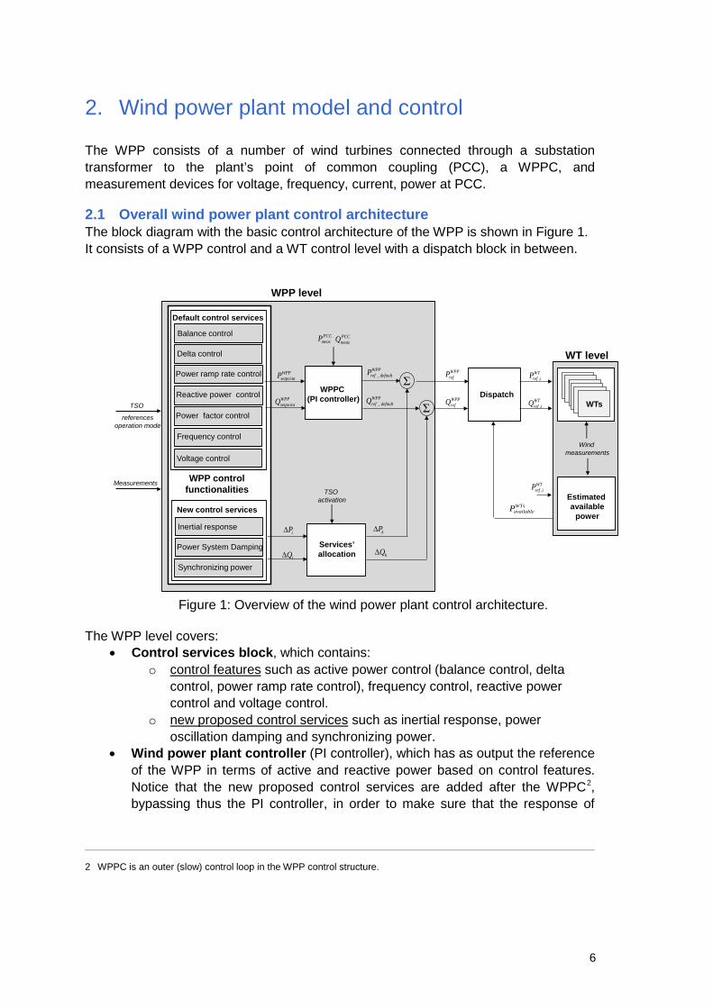
2.1 Overall wind power plant control architecture The block diagram with the basic control architecture of the WPP is shown in Figure 1. It consists of a WPP control and a WT control level with a dispatch block in between.
The WPP level covers: • Control services block, which contains:
o control features such as active power control (balance control, delta control, power ramp rate control), frequency control, reactive power control and voltage control.
o new proposed control services such as inertial response, power oscillation damping and synchronizing power.
• Wind power plant controller (PI controller), which has as output the reference of the WPP in terms of active and reactive power based on control features. Notice that the new proposed control services are added after the WPPC2, bypassing thus the PI controller, in order to make sure that the response of
2 WPPC is an outer (slow) control loop in the WPP control structure.
Figure 1: Overview of the wind power plant control architecture.
v
v
vDispatchv
Inertial response
Synchronizing power
Power System Damping
New control services
Balance control
Frequency control
Delta control
Default control services
Voltage control
Power ramp rate control
Services’allocation
WPPC (PI controller)
Σ
Σ
WPP controlfunctionalities
kP∆
kQ∆
WPPsetpoP int
WPPsetpoQ int
iP∆
iQ∆
WPPrefP
WPPrefQ
WPPdefaultrefP _
WPPdefaultrefQ _ WTs
WTirefP ,
WTirefQ ,
WTsavailableP
TSO activation
Wind measurements
PCCmeasP PCC
measQ
TSO
referencesoperation mode
Measurements
vEstimatedavailable
power
WT level
WPP level
Reactive power control
WTirefP ,
Power factor control
6
these new control services is dependent on the power rate limiter and the controllers placed in the wind turbine level.
• Dispatching block, which distributes the individual power references to the wind turbines.
• Services’ allocation block, which makes possible to select/activate and even combine sequential or simultaneously multiple control functionalities with a specific weighting. The allocation is applied only on the new control services at the present stage.
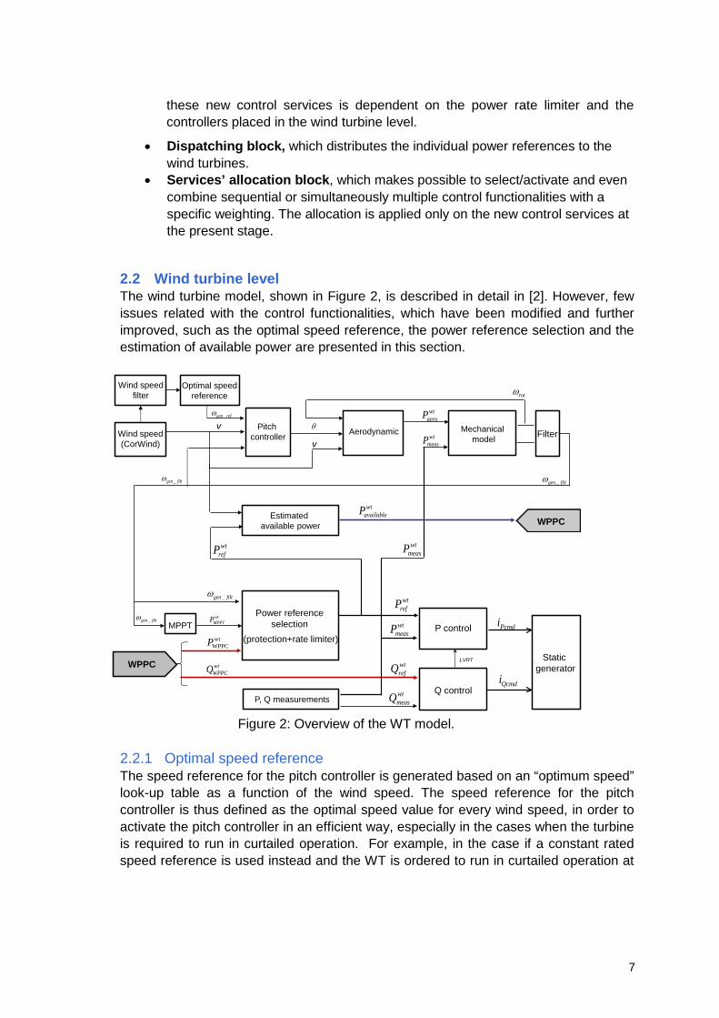
2.2 Wind turbine level The wind turbine model, shown in Figure 2, is described in detail in [2]. However, few issues related with the control functionalities, which have been modified and further improved, such as the optimal speed reference, the power reference selection and the estimation of available power are presented in this section.
2.2.1 Optimal speed reference The speed reference for the pitch controller is generated based on an “optimum speed” look-up table as a function of the wind speed. The speed reference for the pitch controller is thus defined as the optimal speed value for every wind speed, in order to activate the pitch controller in an efficient way, especially in the cases when the turbine is required to run in curtailed operation. For example, in the case if a constant rated speed reference is used instead and the WT is ordered to run in curtailed operation at
Figure 2: Overview of the WT model.
Pitchcontroller Aerodynamic Mechanical
model
Staticgenerator
Wind speed(CorWind)
P, Q measurements
P control
Q control
v
vFilter
MPPTPower reference
selection(protection+rate limiter)
WPPC
WPPC
LVRT
wtWPPCP
Optimal speedreference
Wind speedfilter
filtgen _ω
refgen _ω
filtgen _ω
Estimatedavailable power
filtgen _ω
wtMPPTP
wtrefP
wtmeasP
wtmeasP
wtmeasQ
wtrefQwt
WPPCQ
wtrefP
wtavailableP
Pcmdi
Qcmdi
wtaeroP
wtmeasP
rotω
θ
filtgen _ω
7
low wind speeds, the wind turbine would use the excess power to accelerate up to the rated speed before the pitch controller would be able to pitch to limit the speed.
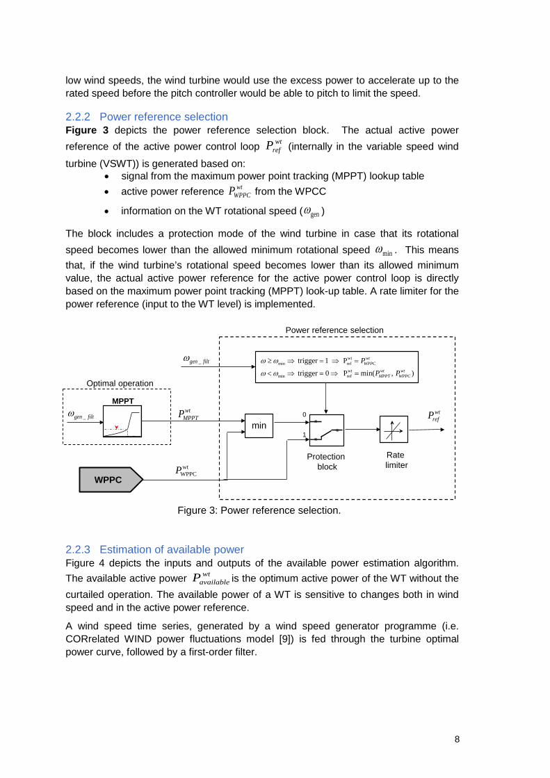
2.2.2 Power reference selection Figure 3 depicts the power reference selection block. The actual active power reference of the active power control loop wt
refP (internally in the variable speed wind
turbine (VSWT)) is generated based on: • signal from the maximum power point tracking (MPPT) lookup table • active power reference wt
WPPCP from the WPCC
• information on the WT rotational speed ( genω )
The block includes a protection mode of the wind turbine in case that its rotational speed becomes lower than the allowed minimum rotational speed minω . This means that, if the wind turbine’s rotational speed becomes lower than its allowed minimum value, the actual active power reference for the active power control loop is directly based on the maximum power point tracking (MPPT) look-up table. A rate limiter for the power reference (input to the WT level) is implemented.
2.2.3 Estimation of available power Figure 4 depicts the inputs and outputs of the available power estimation algorithm. The available active power wt
availableP is the optimum active power of the WT without the curtailed operation. The available power of a WT is sensitive to changes both in wind speed and in the active power reference.
A wind speed time series, generated by a wind speed generator programme (i.e. CORrelated WIND power fluctuations model [9]) is fed through the turbine optimal power curve, followed by a first-order filter.
Figure 3: Power reference selection.
MPPT
Optimal operation),min(P0trigger
P1triggerwtrefmin
wtrefmin
wtWPPC
wtMPPT
wtWPPC
PPP
=⇒=⇒<
=⇒=⇒≥
ωω
ωω
0 wtrefP
1min
Protectionblock
WPPCwt
WPPCP
wtMPPTP
Rate limiter
Power reference selection
filtgen _ω
filtgen _ω
8

2.3 Wind power plant level – control functionalities This section provides an overview of the control features required today by grid codes (GC) [1], of new ancillary services proposed in this document, of WPPC, of the dispatch and allocation of the proposed ancillary services.
2.3.1 Control Features Different control features, which are required by system operators, have been implemented in the WPP level, such as:
• Balance control (absolute power de-rating) o whereby the WPP production can be adjusted downwards or upwards, in steps at constant levels.
• Power ramp rate control o which sets how fast the wind farm power production, can be adjusted
upwards and downwards. • Delta control (power spinning reserve)
o whereby the WPP is ordered to operate with a certain constant reserve capacity in relation to its momentary possible power production capacity.
• Reactive power control o Controls the reactive power in PCC, i.e. WPP is able to produce/absorb a
constant specific amount of reactive power. • Frequency control (governor characteristics)
o controls the frequency in PCC, i.e. WPP produces more or less active power in order to compensate for a deviant behaviour in the frequency.
• Voltage control o controls the voltage at PCC, i.e. WPP is able to produce/absorb reactive
power to/from the grid in order to compensate the deviations of the voltage at PCC.
The fault ride-through (FRT) capability has also been implemented in the WT level as described in [2].
2.3.2 New ancillary services The purpose of this section is to overview the control functionalities for new ancillary services from wind power plants, namely Inertial Response (IR), Power Oscillation Damping (POD) and Synchronizing Power (SP).
Figure 4: Estimation of available power.
v
wtrefP
wtavailableP
Wind speedgenerator(Corwind)
Power referenceselection
Available PowerEstimation
9
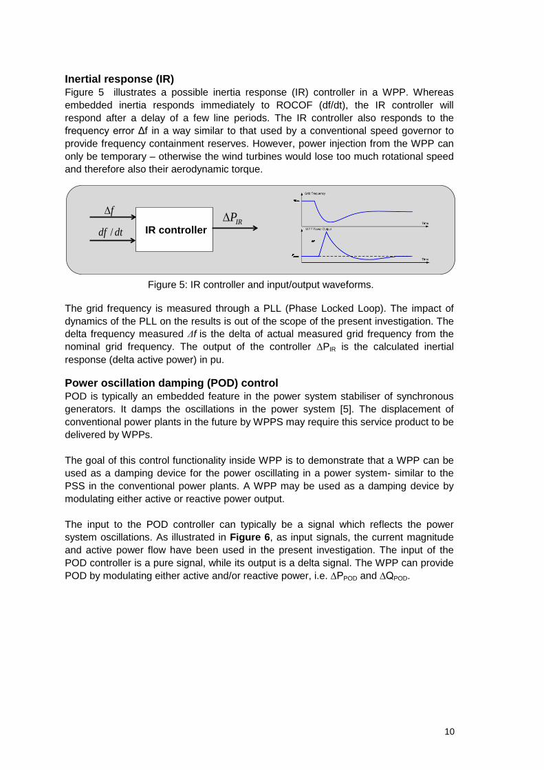
Inertial response (IR) Figure 5 illustrates a possible inertia response (IR) controller in a WPP. Whereas embedded inertia responds immediately to ROCOF (df/dt), the IR controller will respond after a delay of a few line periods. The IR controller also responds to the frequency error Δf in a way similar to that used by a conventional speed governor to provide frequency containment reserves. However, power injection from the WPP can only be temporary – otherwise the wind turbines would lose too much rotational speed and therefore also their aerodynamic torque.
The grid frequency is measured through a PLL (Phase Locked Loop). The impact of dynamics of the PLL on the results is out of the scope of the present investigation. The delta frequency measured Δf is the delta of actual measured grid frequency from the nominal grid frequency. The output of the controller ΔPIR is the calculated inertial response (delta active power) in pu.
Power oscillation damping (POD) control POD is typically an embedded feature in the power system stabiliser of synchronous generators. It damps the oscillations in the power system [5]. The displacement of conventional power plants in the future by WPPS may require this service product to be delivered by WPPs. The goal of this control functionality inside WPP is to demonstrate that a WPP can be used as a damping device for the power oscillating in a power system- similar to the PSS in the conventional power plants. A WPP may be used as a damping device by modulating either active or reactive power output. The input to the POD controller can typically be a signal which reflects the power system oscillations. As illustrated in Figure 6, as input signals, the current magnitude and active power flow have been used in the present investigation. The input of the POD controller is a pure signal, while its output is a delta signal. The WPP can provide POD by modulating either active and/or reactive power, i.e. ∆PPOD and ∆QPOD.
Figure 5: IR controller and input/output waveforms.
IR controllerIRP∆f∆
dtdf /
10

POD controller consists typically of a Wash-Out filter, a Lead-Lag, a Gain and a limiter for the output signal. The Washout filter is filtering the input signal and removes any high order harmonics that are not of interest. The Lead-Lag block is providing the proper phase compensation desired. It consists of two stage phase compensation and a gain that compensate the attenuation at the desired frequency for which the lead-lag is tuned. The gain is scaling the output to obtain the desired contribution for POD control. The reference signal from POD is limited to the available range allocated for POD. Synchronising power (SP) support SP is an embedded feature of synchronous generators, which reduces the load angle between groups of SC in the PS. If the load angle becomes too high, the SGs lose torque and system becomes unstable. An increase in the share of converter connected generators, as the case of WPPs, decreases the amount of the available SP in the system. As result, it may be necessary to introduce SP as a new AS product. The idea of SP from WPP, is thus to improve the steady state stability of the PS by giving additional power into the system from the WPP, in cases when the rotor angle rises above a safe limit. Typically the change in rotor angle is determined by a load change. Based on the rotor or voltage angle deviation the SP controller increases the active power output of the WPP and thus compensate with active power the lack of SP in the system.
The input of the SP controller is a pure signal, while its output is a delta signal. As illustrated in Figure 7, in the present work two different input signals are investigated: rotor angle difference between 2 generators and the voltage angle difference between 2 busbars. Rotor angle of a generator referred to another generator can be calculated using voltage angles and a reduced network model [6], where the generators are connected to. As illustrated in Figure 7 the output of the controller is the delta active power ΔPSP in pu.
Figure 6: POD controller and input/output waveforms.
Figure 7: SP controller and input/output waveforms.
POD controller
Active Power or Current Magnitude
Time
[ Tens of sec]
[ Tens of sec]
WPP Active or Reactive Power output
TimeActive Power Actual or Curtailed
SP controller SPP∆δ∆
θ∆
Load Angle
Time
WPP power output
Time
11
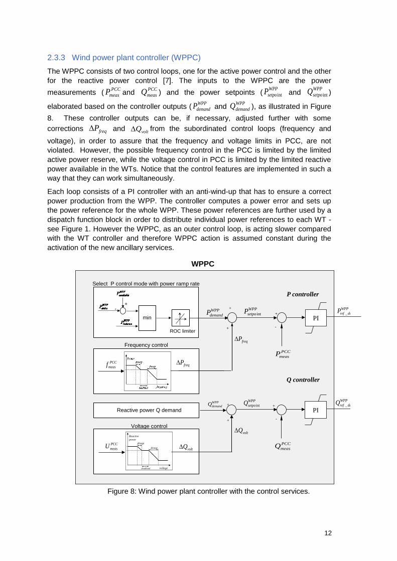
2.3.3 Wind power plant controller (WPPC)
The WPPC consists of two control loops, one for the active power control and the other for the reactive power control [7]. The inputs to the WPPC are the power measurements ( PCC
measP and PCCmeasQ ) and the power setpoints ( WPP
setpoP int and WPPsetpoQ int )
elaborated based on the controller outputs ( WPPdemandP and WPP
demandQ ), as illustrated in Figure 8. These controller outputs can be, if necessary, adjusted further with some corrections freqP∆ and voltQ∆ from the subordinated control loops (frequency and
voltage), in order to assure that the frequency and voltage limits in PCC, are not violated. However, the possible frequency control in the PCC is limited by the limited active power reserve, while the voltage control in PCC is limited by the limited reactive power available in the WTs. Notice that the control features are implemented in such a way that they can work simultaneously.
Each loop consists of a PI controller with an anti-wind-up that has to ensure a correct power production from the WPP. The controller computes a power error and sets up the power reference for the whole WPP. These power references are further used by a dispatch function block in order to distribute individual power references to each WT - see Figure 1. However the WPPC, as an outer control loop, is acting slower compared with the WT controller and therefore WPPC action is assumed constant during the activation of the new ancillary services.
Figure 8: Wind power plant controller with the control services.
+
+
+
-
PCCmeasP
PIWPP
defrefP _
+
+
+
-
PCCmeasQ
PIWPP
defrefQ _
voltQ∆
WPPsetpoQ int
P controller
Q controller
WPPsetpoP int
freqP∆
PCCmeasf freqP∆
Frequency control
Select P control mode with power ramp rate
PCCmeasU
voltage
Reactivepower
droop
droop
deadband
Reactive power Q demandWPPdemandQ
Voltage control
voltQ∆
min
ROC limiter
+- WPP
demandP
WPPC
12
2.3.4 Dispatch Dispatch function block distributes the power references to the wind turbines WT
irefP , , WT
irefQ , (i=1:number of WTs). There are different ways to design the dispatch function. The dispatch function implemented in the present work is based on a proportional distribution of the WPP power setpoints taking into account the estimated available power, respectively:
wtiavailableWPP
available
WPPrefwt
irefwt
iavailableWPPavailable
WPPrefwt
iref QQQ
QPPP
P ,,,, , == (1)
where the total active and reactive power of the wind farm are expressed as follows:
∑∑==
==n
i
WTiavailable
WPPavailable
n
i
WTiavailable
WPPavailable QQPP
1,
1, , (2)
where WTiavailableP , is the available power for the i’th wind turbine. WT
iavailableQ , is the available reactive power of the i’th wind turbine, computed based on the generator rated apparent power for each wind turbine WT
iratedS , , as follows:
2,
2,, )()( WT
iavailableWT
iratedWT
iavailable PSQ −= (3)
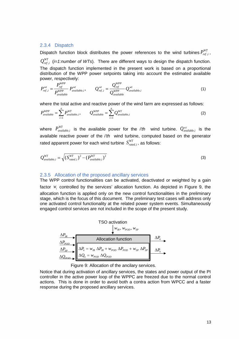
2.3.5 Allocation of the proposed ancillary services The WPP control functionalities can be activated, deactivated or weighted by a gain factor iw controlled by the services’ allocation function. As depicted in Figure 9, the allocation function is applied only on the new control functionalities in the preliminary stage, which is the focus of this document. The preliminary test cases will address only one activated control functionality at the related power system events. Simultaneously engaged control services are not included in the scope of the present study.
Notice that during activation of ancillary services, the states and power output of the PI controller in the active power loop of the WPPC are freezed due to the normal control actions. This is done in order to avoid both a contra action from WPCC and a faster response during the proposed ancillary services.
Figure 9: Allocation of the ancilary services.
Allocation functionIRP∆
PODP∆
SPP∆
PODQ∆
kP∆
kP∆PODPODk
SPSPPODPODIRIRk
QwQPwPwPwP
∆=∆∆+∆+∆=∆
TSO activationSPPODIR www ,,
13

3. WPPC new ancillary services (open loop simulations)
The purpose of this section is to illustrate, by means of open loop s-domain simulations, the results of the implemented new ancillary services in Power Factory simulation tool: inertial response (IR), power oscillation damping (POD) and synchronising power (SP). The section is not targeting to provide an optimal tuning of the controllers, as this is meaningful to be conducted when closed loop simulations will be performed.
The focus is thus on the performance of the WPP output and not the impact of the WPP on the power system. The success criteria of these open loop simulations is that WPP is operating within its control and mechanical limits, while it is providing active or reactive power support through the new ancillary services.
In order to show the performance of the WPP with the new ancillary services, different open loop simulations using a simple power system have been conducted. The simple power system, consisting of a voltage source connected to a wind power plant, is used to verify the performance of the proposed ancillary services in different wind speed conditions and grid events. Different constant wind speeds are applied to the WT model in order to capture the impact of the control features and proposed ancillary services on the WT. It is assumed that an individual WT is simulated in open loop as it is connected to a large power system.
Pre-defined relevant grid events for testing IR, POD, SP in open loop simulations with a simple power system model are generated based on the generic 12-busbar model without wind penetration [3], namely without wind power affecting the grid. These grid events are determined as a generation loss, a short-circuit, and a load increase for IR, POD, and SP, respectively.
Figure 10 sketches the open loop simulation setup with the inputs from the generic 12-bus model no-wind case to the WPP model and the simple power system model. Two measurement files are generated by conducting the simulations of the grid events (i.e. generation loss, short-circuit, and load change) in the generic 12-bus system without wind power penetration: one as input to the WPPC and one as input to the voltage source. These files are required as the measurement signals for the proposed ancillary services. The first measurement file includes the voltage magnitude, angle, and frequency of the PCC bus, which is assumed as the connection point of a WPP in the generic 12-bus system. Accordingly, the second measurement file contains saved signals of the remote bus or line such as active power, current flow, voltage magnitude and angle as an input to the POD and SP ancillary services. It is worth mentioning that all the measurements are recorded directly from Power Factory library blocks (i.e. bus voltage magnitude and current measurement blocks) 3.
3 A realistic implementation approach of the measurements is out of the scope of this work.
14
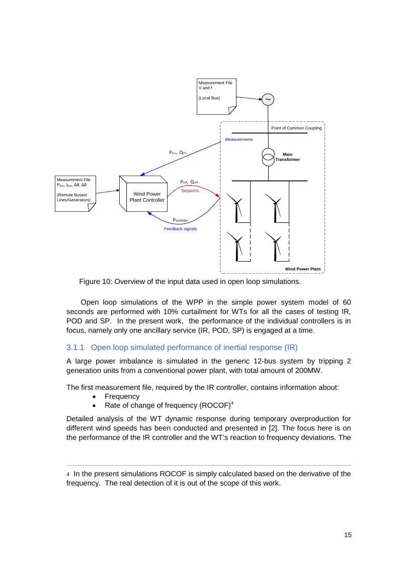
Open loop simulations of the WPP in the simple power system model of 60
seconds are performed with 10% curtailment for WTs for all the cases of testing IR, POD and SP. In the present work, the performance of the individual controllers is in focus, namely only one ancillary service (IR, POD, SP) is engaged at a time.
3.1.1 Open loop simulated performance of inertial response (IR)
A large power imbalance is simulated in the generic 12-bus system by tripping 2 generation units from a conventional power plant, with total amount of 200MW. The first measurement file, required by the IR controller, contains information about:
• Frequency • Rate of change of frequency (ROCOF)4
Detailed analysis of the WT dynamic response during temporary overproduction for different wind speeds has been conducted and presented in [2]. The focus here is on the performance of the IR controller and the WT’s reaction to frequency deviations. The
4 In the present simulations ROCOF is simply calculated based on the derivative of the frequency. The real detection of it is out of the scope of this work.
Figure 10: Overview of the input data used in open loop simulations.
Measurements
Main Transformer
Wind Power Plant
Setpoints
Feedback signals
Point of Common Coupling
~
Wind Power Plant Controller
Measurement File Pline, Iline, Δθ, Δδ
(Remote Buses/Lines/Generators)
Measurement FileV and f
(Local Bus)
PPCC, QPCC
Pref, Qref
Pavailable
15

open loop simulations regarding IR control performance have been also conducted with the frequency droop controller deactivated.
As all simulations are performed with 10% curtailment, the available power is higher than the actual power production, namely the turbine has a certain reserve for contributing with inertial response.
Figure 11 shows the grid frequency excursion followed by the loss of generation and the corresponding IR signal as output of the IR controller.
Figure 12, Figure 13 and Figure 14 depict the electrical power, the generator speed and the pitch angle of the WT for different wind speeds, i.e. low wind speeds (0.6pu wind), near rated wind speed (0.98pu wind) and high wind speed (1.2pu wind), respectively. Notice in all these figures that the rotational speed is decreasing when the grid frequency drops, as result of the IR controller action. The increase in electrical power deteriorates the power imbalance hence the generator speed decreases. The reduction in speed activates the pitch actuation, by decreasing it in order to reduce the imbalance between the electrical power and mechanical power during frequency drop.
Notice that as the turbine is running with 10% curtailment in all these cases, i.e. also for low wind speed, the minimum rotation speed of 0.5pu is not exceeded while delivering the needed extra active power.
Figure 11: IR controller’s input (frequency) and output IRP∆ .
-5 0 5 10 15 20 25 30 35 400.98
0.985
0.99
0.995
1
1.005Frequency [pu]
-5 0 5 10 15 20 25 30 35 40-0.05
0
0.05
0.1
0.15
0.2Inertial response ∆ PIR [pu]
Time [s]
16

Figure 12: WPP performance with IR controller - 0.6pu wind speed,
Figure 13: WPP performance with IR controller - 0.98pu wind speed,
-5 0 5 10 15 20 25 30 35 400.1
0.2
0.3
0.4
0.5WPP active power [pu]
-5 0 5 10 15 20 25 30 35 40
0.8
0.82
0.84
0.86
Generator speed [pu]
-5 0 5 10 15 20 25 30 35 40
0
2
4
6Pitch angle [deg]
Time [s]
-5 0 5 10 15 20 25 30 35 40
0.6
0.8
1
WPP active power [pu]
-5 0 5 10 15 20 25 30 35 400.9
0.95
1
1.05Generator speed [pu]
-5 0 5 10 15 20 25 30 35 40
0
2
4
6
8Pitch angle [deg]
Time [s]
17
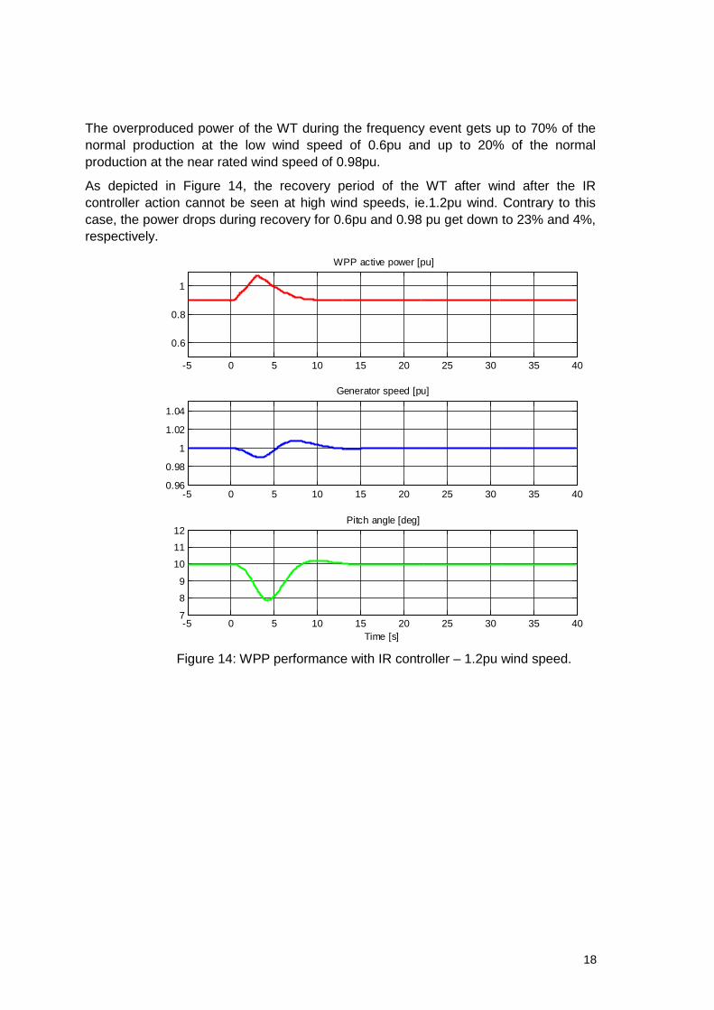
The overproduced power of the WT during the frequency event gets up to 70% of the normal production at the low wind speed of 0.6pu and up to 20% of the normal production at the near rated wind speed of 0.98pu.
As depicted in Figure 14, the recovery period of the WT after wind after the IR controller action cannot be seen at high wind speeds, ie.1.2pu wind. Contrary to this case, the power drops during recovery for 0.6pu and 0.98 pu get down to 23% and 4%, respectively.
Figure 14: WPP performance with IR controller – 1.2pu wind speed.
-5 0 5 10 15 20 25 30 35 40
0.6
0.8
1
WPP active power [pu]
-5 0 5 10 15 20 25 30 35 400.96
0.98
1
1.02
1.04
Generator speed [pu]
-5 0 5 10 15 20 25 30 35 407
8
9
10
11
12Pitch angle [deg]
Time [s]
18

3.1.2 Open loop simulated performance of power oscillation damping (POD)
A set of simulations has been performed in order to illustrate the performance of the POD controller for two different input signals:
• Current magnitude • Active power flow
Different constant wind speeds, i.e. 0.6pu, 0.97pu, 1.2pu, have been considered in order to depict the performance of the WT during POD controller action.
Figure 15 shows the voltage profile during a short circuit event5 for duration of 150msec. Two sets of measurements are recorded from the 12 busbar model to conduct the open loop simulations. The first measurement set contains information about the PCC voltage magnitude and angle, while the second one contains the feedback signals from the remote location (i.e. line 1-6 current magnitude and active power flow) as inputs to the POD controller.
Figure 16 depicts the output of the POD controller when the current magnitude in the Line 1-6 of the 12-bus power system model is used as input POD controller.
5 Short circuit event with a short circuit impedance Zsc (5+j15 ohm)
Figure 15: Voltage profile during the short circuit event.
-5 0 5 10 15 20
0.65
0.7
0.75
0.8
0.85
0.9
0.95
1
1.05
1.1Voltage [pu]
Time [s]
19

Figure 17 depicts the output of the POD controller when the active power flow in the Line 1-6 of the 12-bus power system model is used as input POD controller6.
6 A further tuning of the controller will be conducted during the closed loop simulations.
Figure 16: Input and output in POD controller: current magnitude and PODQ∆
-5 0 5 10 15 200
0.2
0.4
0.6
0.8
1Current magnitude[pu]- input to POD controller
-5 0 5 10 15 20-0.02
0
0.02
0.04
0.06
0.08
0.1
Time [s]
∆ QPOD [pu] - output of POD controller
Zoom
4 4.5 5 5.5 6 6.5 7 7.5 8 8.5 90.12
0.14
0.16
0.18
0.2
0.22
4 4.5 5 5.5 6 6.5 7 7.5 8 8.5 9
-2
0
2
4
6
8
10
12x 10
-3
Time [s]
20
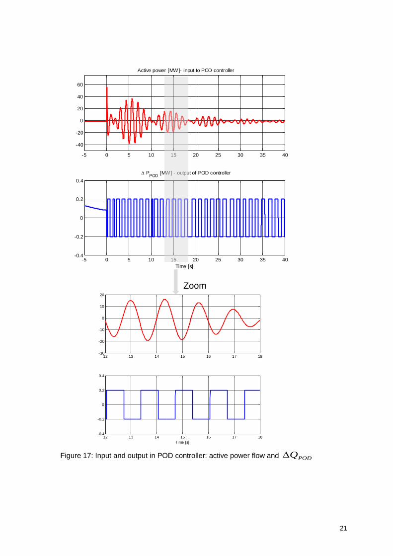
Figure 17: Input and output in POD controller: active power flow and PODQ∆
-5 0 5 10 15 20 25 30 35 40
-40
-20
0
20
40
60
Active power [MW]- input to POD controller
-5 0 5 10 15 20 25 30 35 40-0.4
-0.2
0
0.2
0.4
Time [s]
∆ PPOD [MW] - output of POD controller
Zoom
12 13 14 15 16 17 18-30
-20
-10
0
10
20
12 13 14 15 16 17 18-0.4
-0.2
0
0.2
0.4
Time [s]
21
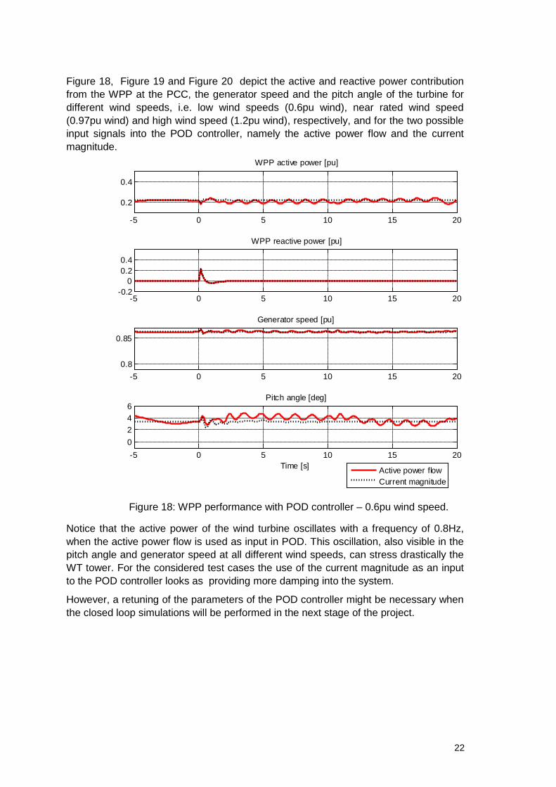
Figure 18, Figure 19 and Figure 20 depict the active and reactive power contribution from the WPP at the PCC, the generator speed and the pitch angle of the turbine for different wind speeds, i.e. low wind speeds (0.6pu wind), near rated wind speed (0.97pu wind) and high wind speed (1.2pu wind), respectively, and for the two possible input signals into the POD controller, namely the active power flow and the current magnitude.
Notice that the active power of the wind turbine oscillates with a frequency of 0.8Hz, when the active power flow is used as input in POD. This oscillation, also visible in the pitch angle and generator speed at all different wind speeds, can stress drastically the WT tower. For the considered test cases the use of the current magnitude as an input to the POD controller looks as providing more damping into the system.
However, a retuning of the parameters of the POD controller might be necessary when the closed loop simulations will be performed in the next stage of the project.
Figure 18: WPP performance with POD controller – 0.6pu wind speed.
-5 0 5 10 15 20
0.2
0.4
WPP active power [pu]
Active power flowCurrent magnitude
-5 0 5 10 15 20-0.2
00.20.4
WPP reactive power [pu]
-5 0 5 10 15 200.8
0.85
Generator speed [pu]
-5 0 5 10 15 200246
Pitch angle [deg]
Time [s]
22
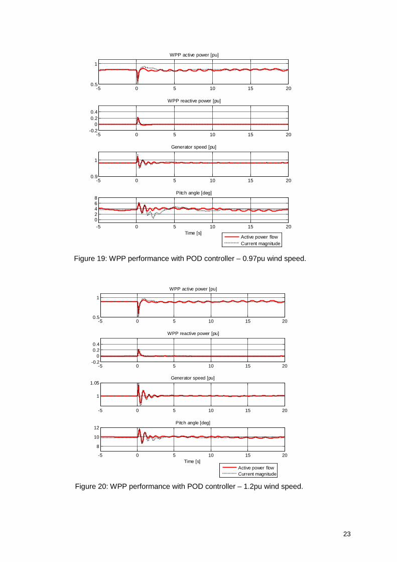
Figure 19: WPP performance with POD controller – 0.97pu wind speed.
Figure 20: WPP performance with POD controller – 1.2pu wind speed.
-5 0 5 10 15 200.5
1
WPP active power [pu]
Active power flowCurrent magnitude
-5 0 5 10 15 20-0.2
00.20.4
WPP reactive power [pu]
-5 0 5 10 15 200.9
1
Generator speed [pu]
-5 0 5 10 15 2002468
Pitch angle [deg]
Time [s]
-5 0 5 10 15 200.5
1
WPP active power [pu]
Active power flowCurrent magnitude
-5 0 5 10 15 20-0.2
00.20.4
WPP reactive power [pu]
-5 0 5 10 15 20
1
1.05Generator speed [pu]
-5 0 5 10 15 20
8
10
12Pitch angle [deg]
Time [s]
23

3.1.3 Open loop simulations for the performance of synchronizing power (SP) In order to analyse the impact of the proposed SP control on the angle stability, a load increase/decrease event is simulated in the generic 12-bus system for duration of 20 sec. As illustrated in Figure 21 the system load in Busbar 4 is ramped up-down 57%, having a simulated duration of five seconds each case.
A set of simulations has been performed in order to illustrate the performance of the SP controller for two different input signals:
• Rotor angle deviation • Voltage angle deviation
Different wind speeds, i.e. 0.6pu, 0.97pu, 1.2pu, have been considered in order to depict the performance of the wind turbine during activation of POD controller.
The load in the PS increases with a ramp while the WPP responds with a power increase due to load angle increase, therefore SG’s rotor angle remains limited. Figure 22 depicts the output of the SP controller when the rotor angle between the generator 2 and 3, when a load change event is generated in Bus4, as indicated in Figure 21, is used as input in the SP controller. Figure 23 depicts the output of the SP controller when the voltage angle between Bus 2 and 3 when a load change event is generated in Bus4, as indicated in Figure 21, is used as input in the SP controller.
Figure 21: Load change profile for testing SP.
0 5 10 15 20 25 30280
300
320
340
360
380
400
420
440
460
480
Time (s)
Load
4 a
t B
us 4
(MW
)
24
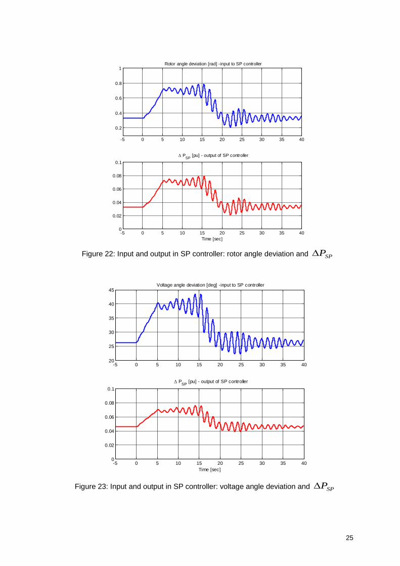
Figure 22: Input and output in SP controller: rotor angle deviation and SPP∆
Figure 23: Input and output in SP controller: voltage angle deviation and SPP∆
-5 0 5 10 15 20 25 30 35 40
0.2
0.4
0.6
0.8
1Rotor angle deviation [rad] -input to SP controller
-5 0 5 10 15 20 25 30 35 400
0.02
0.04
0.06
0.08
0.1∆ PSP [pu] - output of SP controller
Time [sec]
-5 0 5 10 15 20 25 30 35 4020
25
30
35
40
45Voltage angle deviation [deg] -input to SP controller
-5 0 5 10 15 20 25 30 35 400
0.02
0.04
0.06
0.08
0.1∆ PSP [pu] - output of SP controller
Time [sec]
25

Figure 24, Figure 25 and Figure 26 depict the active and reactive power contribution at the PCC from the WPP, the generator speed and the pitch angle of the turbine for different wind speeds, i.e. low wind speeds (0.6pu wind), near rated wind speed (0.97pu wind) and high wind speed (1.2pu wind), respectively, and for the two possible input signals into the SP controller ,(i.e. the rotor angle and the voltage angle deviations).
Notice in Figure 24 that at low wind speeds (i.e. 0.6pu) the WPP is almost using its 10% power reserve, while it is contributing with active power during the activation of SP controller. For all the wind speeds, the increase in active power is as reflected in the decrease of the pitch angle, while the generator speed is almost unchanged. During SP action the WPP also injects reactive power into the system, this being largest at low wind speeds.
It is worth noticing that there is no significant difference in the performance of the WT in using rotor angle or voltage angle as input in the SP controller.
Figure 24: WPP performance with SP controller – 0.6pu wind speed.
-5 0 5 10 15 20 25 30 35 400.1
0.2
0.3
0.4
0.5WPP active power [pu]
Rotor angleVoltage angle
-5 0 5 10 15 20 25 30 35 400.855
0.86
0.865
0.87Generator speed [pu]
-5 0 5 10 15 20 25 30 35 40
0
2
4
6Pitch angle [deg]
Time [s]
26
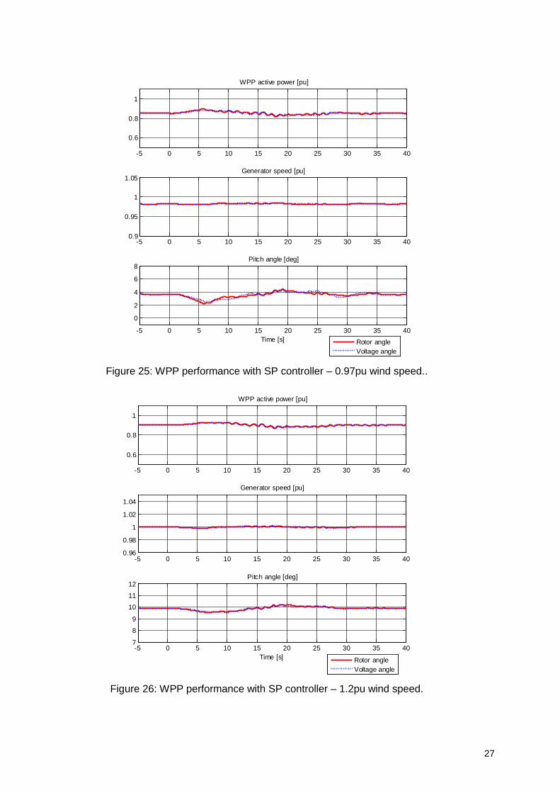
Figure 25: WPP performance with SP controller – 0.97pu wind speed..
Figure 26: WPP performance with SP controller – 1.2pu wind speed.
-5 0 5 10 15 20 25 30 35 40
0.6
0.8
1
WPP active power [pu]
Rotor angleVoltage angle
-5 0 5 10 15 20 25 30 35 400.9
0.95
1
1.05Generator speed [pu]
-5 0 5 10 15 20 25 30 35 40
0
2
4
6
8Pitch angle [deg]
Time [s]
-5 0 5 10 15 20 25 30 35 40
0.6
0.8
1
WPP active power [pu]
Rotor angleVoltage angle
-5 0 5 10 15 20 25 30 35 400.96
0.98
1
1.02
1.04
Generator speed [pu]
-5 0 5 10 15 20 25 30 35 407
8
9
10
11
12Pitch angle [deg]
Time [s]
27

3.1.4 Conclusions for open loop simulations The open loop simulation results have shown that the WPP with IR, POD and SP controllers can contribute to power system stability during disturbances and their performances do not exceed WT’s capabilities. The simulation results perform as expected according to the control structure together with the parameters. However, the impact of the pitch system model and the parameters of the new ancillary services on the performance of the WT are of high importance. This will be particularly investigated in the closed loop simulations, which will be conducted and presented in the next report.
4. Comparison of aggregated WPP model with detailed WPP model
4.1 Wind power plant electrical layout (simple power system) The WPP layout corresponding to a detailed WPP model implemented in PowerFactory for the aggregation study propose is shown in Figure 27a. It includes 8 individual wind turbines placed in two rows; each consists of 4 wind turbines. The electrical layout of each turbine is depicted in Figure 27b.
Figure 27: a) Wind power plant electrical layout
b) Wind turbine electrical layout.
Main Transformer
PCC
~
33kV
230kV
230kV
WT1
WT2
WT3
WT4 WT5
WT6
WT7
WT8
33kV
33kV
33kV
33kV
33kV
33kV
33kV
G
Static generator
0.96kV
0.96kV
33kVPoC
Wind power plant layout Wind turbine layout
a) b)
28
The WT model includes detailed representation of the turbine’s relevant components and control algorithms, allowing implementation of new control functionalities, if necessary, as described in [2].The WPP is modeled in detail complete set, including individual WTs with their transformers, cables, feeders and main transformer. 8 WTs of 2MW are connected in two-feeder arrangement giving a total capacity of 16 MW. The distance between the turbines is around 500 m. The cables in the WPP are selected in order to obtain a nominal loss of 1% of rated power. With this, the voltage profile remains inside nominal range (±5%).
4.2 Wind speed time series The turbulent wind speed conditions for the individual wind turbines in the detailed WPP model are generated using CorWind model [8].
The CORrelated WIND power fluctuations (CorWind) model has been developed at DTU Wind Energy. It is a software tool that allows the simulation of wind power time series that have a realistic variability. Furthermore, CorWind can simulate wind power output in different locations, taking into account the spatial correlation between them.
CorWind is an extension of the linear and purely stochastic PARKSIMU model [9], which simulates stochastic wind speed time series for individual WTs in a WPP, with fluctuations of each time series according to specified power spectral densities and with correlations between the different wind turbine time series according to specified coherence functions. The coherence functions depend on frequency and space, ensuring that the correlation between two wind speed time series will decrease with increasing distance between the points. Moreover, the slow wind speed fluctuations are more correlated than the fast fluctuations. Finally, the stochastic PARKSIMU model includes the phase shift between correlated waves in downstream points, ensuring that correlated wind speed variations will be delayed in time as they travel through the wind farm. These model properties ensure that the summed power from multiple wind turbines will have realistic fluctuations, which has been validated using measured time series of simultaneous wind speeds and power from individual wind turbines in two large wind farms in Denmark [10].
The CorWind extension of PARKSIMU is intended to allow simulations over large areas and long time periods. The linear approach applied in PARKSIMU assumes constant mean wind speeds and constant mean wind directions during a simulation period, which limits the geographical area as well as the simulation period significantly–typically to the area of a single wind farm and to a maximum period of two hours. CorWind uses reanalysis data from a climate model to provide the mean wind flow over a large region, and then adds a stochastic contribution using an adapted version of the PARKSIMU approach that allows the mean flow to vary in time and space. The layout of the considered wind farm is shown in Figure 28.
29
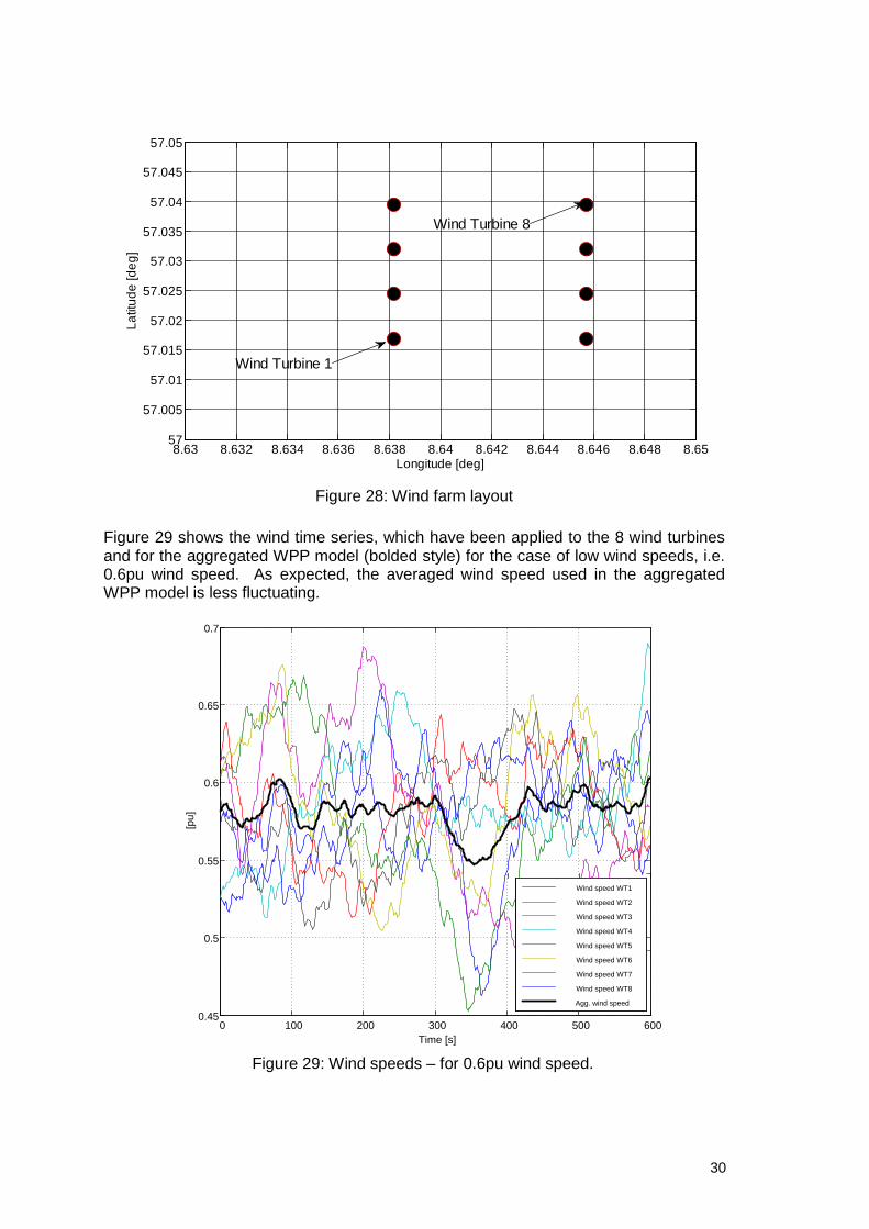
Figure 28: Wind farm layout
Figure 29 shows the wind time series, which have been applied to the 8 wind turbines and for the aggregated WPP model (bolded style) for the case of low wind speeds, i.e. 0.6pu wind speed. As expected, the averaged wind speed used in the aggregated WPP model is less fluctuating.
8.63 8.632 8.634 8.636 8.638 8.64 8.642 8.644 8.646 8.648 8.6557
57.005
57.01
57.015
57.02
57.025
57.03
57.035
57.04
57.045
57.05
Longitude [deg]
Latit
ude
[deg
]
Wind Turbine 1
Wind Turbine 8
Figure 29: Wind speeds – for 0.6pu wind speed.
0 100 200 300 400 500 6000.45
0.5
0.55
0.6
0.65
0.7
Time [s]
[pu]
Wind speed WT1
Wind speed WT2
Wind speed WT3
Wind speed WT4
Wind speed WT5
Wind speed WT6
Wind speed WT7
Wind speed WT8
Agg. wind speed
30
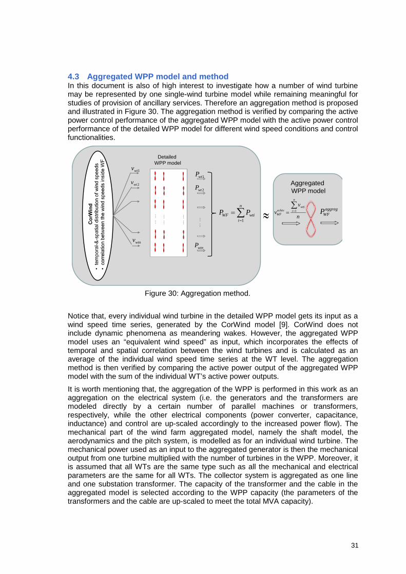
4.3 Aggregated WPP model and method In this document is also of high interest to investigate how a number of wind turbine may be represented by one single-wind turbine model while remaining meaningful for studies of provision of ancillary services. Therefore an aggregation method is proposed and illustrated in Figure 30. The aggregation method is verified by comparing the active power control performance of the aggregated WPP model with the active power control performance of the detailed WPP model for different wind speed conditions and control functionalities.
Notice that, every individual wind turbine in the detailed WPP model gets its input as a wind speed time series, generated by the CorWind model [9]. CorWind does not include dynamic phenomena as meandering wakes. However, the aggregated WPP model uses an “equivalent wind speed” as input, which incorporates the effects of temporal and spatial correlation between the wind turbines and is calculated as an average of the individual wind speed time series at the WT level. The aggregation method is then verified by comparing the active power output of the aggregated WPP model with the sum of the individual WT’s active power outputs.
It is worth mentioning that, the aggregation of the WPP is performed in this work as an aggregation on the electrical system (i.e. the generators and the transformers are modeled directly by a certain number of parallel machines or transformers, respectively, while the other electrical components (power converter, capacitance, inductance) and control are up-scaled accordingly to the increased power flow). The mechanical part of the wind farm aggregated model, namely the shaft model, the aerodynamics and the pitch system, is modelled as for an individual wind turbine. The mechanical power used as an input to the aggregated generator is then the mechanical output from one turbine multiplied with the number of turbines in the WPP. Moreover, it is assumed that all WTs are the same type such as all the mechanical and electrical parameters are the same for all WTs. The collector system is aggregated as one line and one substation transformer. The capacity of the transformer and the cable in the aggregated model is selected according to the WPP capacity (the parameters of the transformers and the cable are up-scaled to meet the total MVA capacity).
Figure 30: Aggregation method.
aggregWFP
n
vv
n
iwti
echivWF
∑== 1
AggregatedWPP model
≈∑=
=n
iwtiWF PP
1
1wtP
2wtP
wtnP
1wtv
2wtv
wtnv
DetailedWPP model
31

Figure 29 shows the wind time series, which have been applied to the 8 wind turbines and for the aggregated WPP model (bolded style) for the case of low wind speeds, i.e. 0.6pu wind speed. As expected, the equivalent wind speed used in the aggregated WPP model is less fluctuating.
4.4 Comparison of the simulation results – aggregation versus detailed model
To verify the accuracy of the proposed aggregation method, a set of dynamic simulation studies is carried out for two different wind speed levels (i.e. low wind speed and near rated wind speed).
4.4.1 Control Features
In this study, the comparison between the aggregated and the detailed WPP model is only focusing on the active power dynamic response in normal operation during maximum possible production as well as when specific control actions, like balance and delta control, are imposed and activated in the WPP. Figure 31 illustrates the active power comparison for the case of 0.6pu wind speed time series.
Figure 31: Active power comparison– for 0.6pu wind speed.
100 200 300 400 500 6003
3.5
4
4.5
5
Act
ive
pow
er [M
W]
p p
100 200 300 400 500 600
0
2
4
6
Act
ive
pow
er e
rror
(%
)
Time [s]
Detailed WPP model
Aggregated WPP model
32

Notice that for these low winds speed time series the active power error between the aggregated WPP model and the detailed WPP model is smaller than 3%. The aggregation method slightly underestimates the active power comparing with that provided by the detailed WPP model.
Figure 32 illustrates the active power comparison for the case of a 0.97pu wind speed, namely near rated wind speed. In this case, the WT is running in the transition between the operational modes of power optimization and power limitation, which is known to be highly challenging from a control point of view. Notice that, for this critical operational condition, i.e. wind speeds near rated wind speed, the active power error between the two models is a bit larger than the previous case, however smaller than 6%. Notice that, in this case, the aggregation method slightly overestimates the active power comparing with the detailed WPP model.
The characteristic of the power curve at the WT operational point for a low wind speed (such as 0.6pu) is different than that for a wind speed near to rated wind speed (such as 0.97pu). This difference can be the reason for the slight underestimation and overestimation of the active power of the aggregated WPP model for 0.6pu and 0.97pu wind speed, respectively, as indicated in Figure 31 and Figure 32. At low wind speeds, where the power curve is very steep, a higher level of turbulence in the wind speed (as it is the case of wind speed series used in the detailed WPP model compared to the average equivalent wind speed used in the aggregated WPP model) can yield to a higher local power production than that corresponding to an average, less fluctuating equivalent wind speed. The situation is slightly different near to the rated wind speed, as here the fluctuations in wind speeds have mostly impact on lowering the power
Figure 32: Active power comparison– for 0.97pu wind speed.
100 200 300 400 500 60012
14
16
18
Act
ive
pow
er [M
W]
p p
100 200 300 400 500 600
0
2
4
6
Act
ive
pow
er e
rror
(%
)
Time [s]
Aggregated WPP model
Detailed WPP model
33
production compared to the case when an average, less fluctuating equivalent wind speed is used.
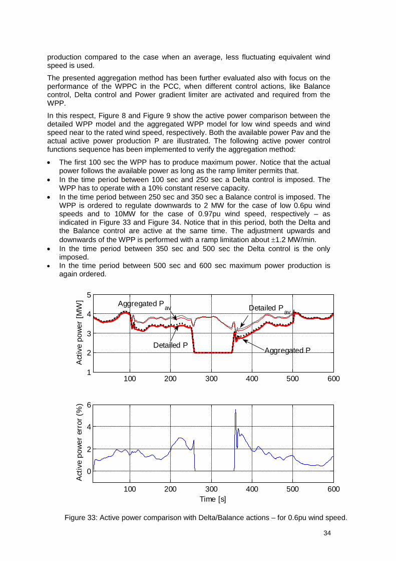
The presented aggregation method has been further evaluated also with focus on the performance of the WPPC in the PCC, when different control actions, like Balance control, Delta control and Power gradient limiter are activated and required from the WPP.
In this respect, Figure 8 and Figure 9 show the active power comparison between the detailed WPP model and the aggregated WPP model for low wind speeds and wind speed near to the rated wind speed, respectively. Both the available power Pav and the actual active power production P are illustrated. The following active power control functions sequence has been implemented to verify the aggregation method:
• The first 100 sec the WPP has to produce maximum power. Notice that the actual power follows the available power as long as the ramp limiter permits that.
• In the time period between 100 sec and 250 sec a Delta control is imposed. The WPP has to operate with a 10% constant reserve capacity.
• In the time period between 250 sec and 350 sec a Balance control is imposed. The WPP is ordered to regulate downwards to 2 MW for the case of low 0.6pu wind speeds and to 10MW for the case of 0.97pu wind speed, respectively – as indicated in Figure 33 and Figure 34. Notice that in this period, both the Delta and the Balance control are active at the same time. The adjustment upwards and downwards of the WPP is performed with a ramp limitation about ±1.2 MW/min.
• In the time period between 350 sec and 500 sec the Delta control is the only imposed.
• In the time period between 500 sec and 600 sec maximum power production is again ordered.
Figure 33: Active power comparison with Delta/Balance actions – for 0.6pu wind speed.
100 200 300 400 500 6001
2
3
4
5
Act
ive
pow
er [M
W]
100 200 300 400 500 600
0
2
4
6
Act
ive
pow
er e
rror
(%
)
Time [s]
Aggregated Pav Detailed Pav
Detailed PAggregated P
34
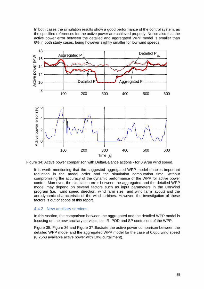
In both cases the simulation results show a good performance of the control system, as the specified references for the active power are achieved properly. Notice also that the active power error between the detailed and aggregated WPP model is smaller than 6% in both study cases, being however slightly smaller for low wind speeds.
It is worth mentioning that the suggested aggregated WPP model enables important reduction in the model order and the simulation computation time, without compromising the accuracy of the dynamic performance of the WPP for active power control. Moreover, the simulation error between the aggregated and the detailed WPP model may depend on several factors such as input parameters in the CorWind program (i.e. wind speed direction, wind farm size and wind farm layout) and the aerodynamic characteristic of the wind turbines. However, the investigation of these factors is out of scope of this report.
4.4.2 New ancillary services
In this section, the comparison between the aggregated and the detailed WPP model is focusing on the new ancillary services, i.e. IR, POD and SP controllers of the WPP.
Figure 35, Figure 36 and Figure 37 illustrate the active power comparison between the detailed WPP model and the aggregated WPP model for the case of 0.6pu wind speed (0.25pu available active power with 10% curtailment).
Figure 34: Active power comparison with Delta/Balance actions - for 0.97pu wind speed.
100 200 300 400 500 6008
10
12
14
16
18
Act
ive
pow
er [M
W]
100 200 300 400 500 600
0
2
4
6
Act
ive
pow
er e
rror
(%
)
Time [s]
Detailed P Aggregated P
Detailed PavAggregated Pav
35

Figure 35: Active power comparison during IR control action - for 0.6pu wind speed.
Figure 36: Active power comparison during POD control action - for 0.6pu wind speed.
0 2 4 6 8 10 12 14 16 18 203
3.5
4
4.5
5
5.5
6
6.5
Act
ive
Pow
er (M
W)
Act
ive
Pow
er (M
W)
Time (s)Time (s)
PWF_av (Available power)
PWF_PCC (Active power output of aggregated model)
PWF_PCC (Active power output of detailed model)
-5 0 5 10 15 20 25 30 35 403.3
3.4
3.5
3.6
3.7
3.8
3.9
4
PWF_av (Available power)
PWF_PCC (Active power output of aggregated model)
PWF_PCC (Active power output of detailed model)
Act
ive
Pow
er (M
W)
Act
ive
Pow
er (M
W)
Time (s)Time (s)
36
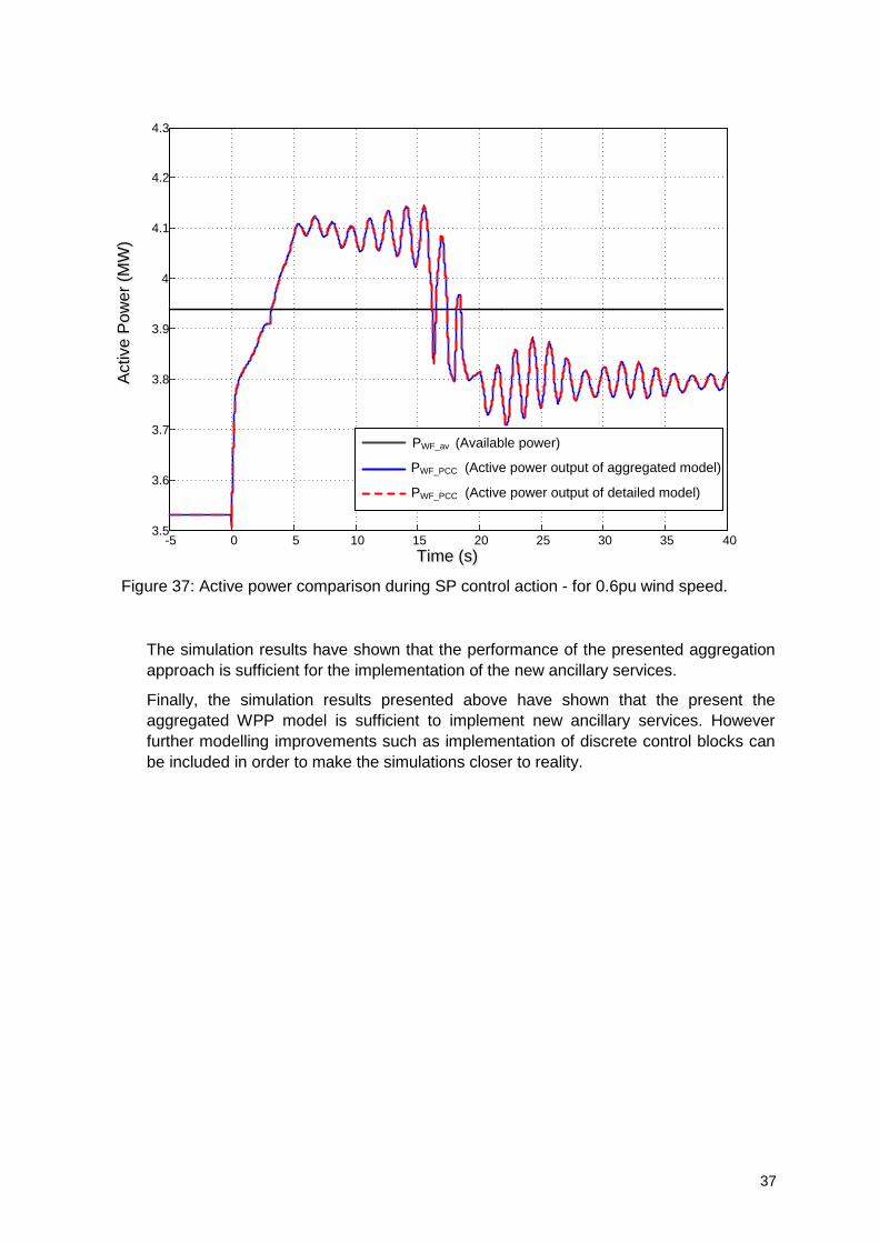
The simulation results have shown that the performance of the presented aggregation approach is sufficient for the implementation of the new ancillary services.
Finally, the simulation results presented above have shown that the present the aggregated WPP model is sufficient to implement new ancillary services. However further modelling improvements such as implementation of discrete control blocks can be included in order to make the simulations closer to reality.
Figure 37: Active power comparison during SP control action - for 0.6pu wind speed.
-5 0 5 10 15 20 25 30 35 403.5
3.6
3.7
3.8
3.9
4
4.1
4.2
4.3
PWF_av (Available power)
PWF_PCC (Active power output of aggregated model)
PWF_PCC (Active power output of detailed model)
Act
ive
Pow
er (M
W)
Act
ive
Pow
er (M
W)
Time (s)Time (s)
37

Acknowledgements
This work was carried out by the DTU Wind Energy Department in cooperation with Vestas Wind Systems A/S and Aalborg University. Energinet.dk is acknowledged for funding this work in contract number: PSO project 2011 no. 10653: ““Enhanced Ancillary Services from Wind Power Plants” (EaseWind).
38

DTU Wind Energy is a department of the Technical University of Denmark with a unique integration of research, education, innovation and public/private sector consulting in the field of wind energy. Our activities develop new opportunities and technology for the global and Danish exploitation of wind energy. Research focuses on key technical-scientific fields, which are central for the development, innovation and use of wind energy and provides the basis for advanced education at the education. We have more than 230 staff members of which approximately 60 are PhD students. Research is conducted within 9 research programmes organized into three main topics: Wind energy systems, Wind turbine technology and Basics for wind energy.
Technical University of Denmark DTU Vindenergi Brovej Building 118 2800 Kgs. Lyngby Denmark Telefon 45 25 17 00 [email protected] www.vindenergi.dtu.dk