Modelling pandemics of quarantine pests and diseases: problems

CROP P R O T E C T I O N (1987) 6 (4), 211-221

Modelling pandemics of quarantine pests and diseases: problems and perspectives

J. A. P. HEESTERBEEK AND J. C. ZADOKS

Laboratory of Phytopathology, Binnenhaven 9, 6709 PD Wageningen, The Netherlands

ABSTRACT. TO develop a general framework for a mathematical theory of pandemics, known facts about pandemics of plant diseases are reconsidered. A pandemic is thought to consist of three parts called zero-order, first-order and second-order epidemics. The zero-order epidemic is the spread of a disease within the boundaries of a single crop field; it includes the establishment of an initial focus and of daughter foci. The first-order epidemic is the spread of a disease over an area with many fields during a single growing season of the host crop. The second-order epidemic is the spread of a disease over a large area during consecutive growing seasons of the host crop. The mathematical description of a second-order epidemic is supposed to lead to a travelling wave solution, the wave travelling at its highest and constant speed during the middle part of the second-order epidemic. Selected empirical evidence supports this hypothesis. Whereas the zero-order and first-order epidemics can be described as continuous processes, the second-order epidemic cannot because of crop seasonality. Comparisons are drawn between botanical and medical epidemiology. The approach taken is deterministic; stochasticity of epidemiological processes is disregarded in this paper.

Everything should be made as simple as possible, but not simpler. A. Einstein

Introduction

A special class of plant 'pests' (in the general sense, including diseases) is called here 'quarantine pests'. The distinguishing characteristics of these pests and diseases are (1) their presence in one area; (2) their absence from another area; (3) the great economic loss they might cause after attaining the latter area. Plant protection services try to keep quarantine pests out of the area under their jurisdiction. Once a quarantine pest has gained access to a new area, notwithstanding plant quarantine measures, plant protection services may attempt to eradicate the pest or, if unsuccessful, to 'contain' it. When eradication and containment fail, the pest may spread rapidly over a whole continent. Crops hitherto unexposed to the new invader usually have little resistance, all varieties being about equally susceptible.

An epidemic which expands over a continent is called a 'pandemic' (Gaeumann, 1946). Some pests of known or expected economic importance are classified as quarantine pests, with all concomitant legal measures, because it is feared that they would cause

severe losses after introduction into new areas. There are numerous historical examples of epidemics and pandemics (Klinkowski, 1970), but very few records of successful eradication.

Estimation of the relative danger posed by a quarantine pest and the design of emergency measures for eradication and containment would profit from models of pandemics with at least some predictive value (McGregor, 1978). Such models should high- light essential features common to many pandemics. These models should provide parameters which can be measured appropriately to fulfil the 'requirement of measurability'. Given these parameters, the models should predict future events, among them the rate of expansion of a pandemic once the quarantine pest has entered a new continent.

Before modelling can be undertaken, at least rudi- mentary theoretical knowledge about the biological system to be modelled must be available. For pandemics, such knowledge is difficult to find in the literature. This paper tries to provide a theoretical basis for the study of pandemics and to investigate the difficulties in modelling them, but it does not consider the stochastic nature of epidemiological events. The paper is limited to diseases caused by fungi, but several ideas are applicable to other classes of 'pests'.

0261-2194/87/04/0211-11 $03.00 © 1987 Butterworth & Co (Publishers) Ltd

212

Available theory

Many different models and modelling approaches exist in epidemiology. Most were developed by mathe- maticians; some were more or less specifically tailored to botanical or medical situations. This section gives a short overview of relevant literature in mathematical modelling.

The moment that a propagule of a pathogen, coming from outside, enters and successfully infects a susceptible crop, hitherto uninfected, an epidemic process is initiated. If circumstances are favourable, an epidemic will develop in time and space. Although temporal and spatial development go together, it is useful to distinguish the two. Temporal development is the increase with time of the number of diseased entities (plants, leaves, sites) or of the fraction of diseased plant material. The apparent infection rate is expressed in entities per entity per unit of time or in a fraction per unit of time, with dimension [ T -1] (Van der Plank, 1963). Spatial development is the increase with time of the area occupied by diseased entities. The rate of area expansion is expressed in units of area per unit of time, dimension [L 2. T-1]. The spatial and temporal aspects of an epidemic relate as extensifica- tion and intensification of the same process (compare Zadoks and Kampmeijer, 1977).

Botanical epidemiology

Van der Plank (1963) initiated many studies in the theory of botanical epidemiology. In these studies, the temporal development of an epidemic within a crop received by far the most attention. Kranz (1974), Zadoks (1979), Gilligan (1985), Teng (1985), and others reviewed mathematical contributions to botanical epidemiology. Contributions were made by Madden (1980), Jeger (1983, 1986), Aylor (1986), McLean, Garrett and Ruesink (1986) and others.

Comparatively few studies have been devoted to spatial development of epidemics within crops. The work on disease gradients by Gregory (1968), on spore cloud trajectories by Schroedter (1960), and infection probabilities by Waggoner (1962) merit attention. Studies that really dealt with focus expansion in the field (Kiyosawa, 1976; Kampmeijer and Zadoks, 1977; Mackenzie, 1979) applied simulation techniques only. Recently, attempts have been made to model spatial development mathematically (Jeger, 1983; Minogue and Fry, 1983a, b; Van den Bosch, Metz and Zadoks, 1987a, b). The attempts by.Minogue and Fry and by Van den Bosch and co-workers, formulated independently, are closely related. Van den Bosch and his colleagues gave a generalized model for the focus expansion of a fungal disease with a sound theoretical basis, suitable for calculation of the propagation rate of the epidemic wave. 'Epidemic wave' is the term used to describe the expanding front of the focal epidemic, when the centre of the focus reaches saturation (Kampmeijer and Zadoks, 1977, p. 34). The spatial

Modelling pandemics of quarantine pests and diseases

development models mentioned are confned to focus expansion within the borders of a single field. Little theoretical work is known on spatial development beyond the borders of one field, on a continental or even regional scale. An early contribution on large- scale dispersal of plants and animals was made by Skellam (1951).

Medical epidemiology

Mathematical modelling of epidemics in medicine has flourished. Bailey (1980) has provided a review of the major approaches and an extensive guide to the literature. Although the majority of the models are specific for given classes of diseases, some models of a general nature could be translated and applied to the botanical situation, mutatis mutandis. The approach developed by Thieme (1977) and Diekmann (1978) has already been followed successfully in botanical epidemiology by Van den Bosch et al. (1987a,b). Other recent developments that could be of future use in botanical epidemiology have been published by Rad- cliffe and Rass (1984) and by Busenberg, Cooke and Pozio (1983).

A new classification of epidemics

In this section a new terminology for botanical epidemics is introduced. The pandemic is divided into three subprocesses called the zero-, first- and second- order epidemics. The three orders of epidemics have different characteristics (Table 1) and each order gives rise to its own specific difficulties in modelling.

Classification

The pandemic is a complex process, in which subprocesses can be distinguished which operate at different levels of complexity and at various scales of time and distance (Zadoks and Schein, 1979, chapter 9). To model an epidemic within a crop, the smallest entity (or individual component) of the host to be considered is a plant, a leaf, or a site (the area occupied by one lesion). The individual component of the pathogen to be considered is a propagule, an entity (spore, mycelial fragment) by which a fungus is dispersed. The individual of disease to be considered is the lesion, the part of the host plant colonized by a single successful propagule. Whereas one propagule

TABLE 1. Characteristics of the three orders of botanical epidemics

Epidemic

Scale Zero-order First-order Second-order

Time

Distance

Within one year Within one year Over many years (monoetic) (monoetic) (polyetic)

Within one field Over many Over whole fields, within continent part of continent

CROP P R O T E C T I O N Vol. 6 August 1987

J. A. P. HEESTERBEEK AND J. C. ZADOKS

cannot produce more than one lesion, one lesion can produce many propagules.

To model a pandemic, the individual component to be considered here is a farmer's field. For the present purpose, a field is a homogeneous piece of land bearing a single, uniform crop cultivar. Each field has its own cropping history. The terms healthy, infected and infectious are now applied to fields. In the present context, an infectious field is a field from which propagules are dispersed to other fields.

A zero-order epidemic is defined as the spread of a disease within the boundaries of a single field. The expansion of a focus within a field is part of the zero- order epidemic, as is the establishment of daughter foci within the same field. A zero-order epidemic is limited to a single growing season. A first-order epidemic is defined as the spread of a disease over an area with many fields during a single growing season of the host crop. A second-order epidemic is defined as the spread of a disease over a large area during consecutive growing seasons of the host crop; it is a polyetic epidemic, sensu Zadoks and Schein (1979).

The first-order epidemic. The following description of the spatial development of an idealized pandemic elaborates on these definitions in abstract terms. A fungal disease F enters a field with crop C. The area containing all fields bearing C, that is the area enclosed by a curve surrounding all fields with C, will be called fL We regard f~ as the set of all farmers' fields (with C and with non-C) within that curve. Its actual area is represented by a number denoted as ]ft [. The number of fields in fZ with crop C is denoted by CO. As F is a quarantine pest, all cultivars of C are assumed to be equally susceptible. We assume that F arrives in fZ in one field only at some time during the growing season of year 1. The first infected field is called the (primary) source field B. I f circumstances are favourable for the development of the disease caused by F, a zero-order epidemic will develop in B. The infectious plants in B release propagules that are dispersed. Each propagule belongs to one of four groups: (1) propagules that fall on the ground; (2) propagules that fall on neighbouring plants; (3) propagules deposited elsewhere in B, and (4) propagules blown out of field B. Only groups (2) and (3) are relevant to the zero-order epidemic. For higher- order epidemics, group (4) is relevant, in so far as these propagules arrive at and infect other fields of C in ~2. With the advance of the season, more plants in B will become infected and more propagules will leave B.

The first propagule from B, which infects another field bearing C, initiates the first-order epidemic. The infection gives rise to a zero-order epidemic in that field, which later will emit propagules of its own. The polycyclic nature of this process leads to a first-order epidemic with increasing rate of progress. The increase with time in the number of fields (Van der Plank, 1963) or greenhouses (Schepers, 1984) may follow the logistic equation. A first-order epidemic consists of many zero-order epidemics, one per

213

infected field. A zero-order epidemic progresses until the infection

level reaches the 'asymptotic value of disease' (Jeger, 1986), or until harvest at the end of the growing season, whichever comes first. A first-order epidemic usually progresses until harvest time. The area containing all fields infected by F during year 1 will be indicated as fZl with area [~'21 ]. The number of infected fields in fZ~ is indicated as co I.

Pathogen survival. When C has disappeared from the fields, F must survive the ensuing crop-free period. In principle, F could be present and viable at all COl fields at the beginning of the growing season in year 2; in practice, this may not be so, first because much of F dies during the adverse off-season, and second, because of crop rotation the C fields in year 2 will usually be near to but different from the C fields of year 1, and part o f F will fail to attain the new fields. The fraction of fields in year 1 with successful carry-over of inoculum to year 2 is a variable indicated as ql. The number of source fields in year 2 will then be q~ x col, assuming co to be constant. In these fields, the zero- order epidemics of year 2 will begin. By emitting propagules these fields will initiate the first-order epidemic of year 2. At the end of the growing season of year 2, F will be present in co2 fields contained within the circumference of area ~22.

The second-order epidemic. In year 1, q0 and COo are assumed to be 1. A pandemic can develop only if ql x col >q0 x coo, when mean field size is constant over the years. If so, the first-order epidemic in year 2 starts with more source fields than that in year 1. Conse- quently, the first-order epidemic of year 2 will develop faster than that of year 1. When successive growing seasons i are approximately equal, the area encompas- sing all infected fields expands: ~21C~22 and [~22 [> [f~ [. Other things remaining equal this implies co2>co~. At the beginning of year 3 there will be q2Xco2 source fields. The second-order epidemic of F on C in ~2 continues as long as [~2k ]> [~2i [ for all k>i. Once ~2k = ~2 i for all k >i, the pandemic comes to a standstill.

Endemicity is defined here as the property of a pest to survive in a certain area, being able to cause occasional outbreaks in that area (Zadoks and Schein, 1979). The area, here denoted as fZE, is the part of~2 where environmental conditions are such that F can coexist with C (compare Carter and Prince, 1981), ~EC__~ and [~E 1< [~'2 [. Equality is possible only when F can survive the off-season at all places where C is grown. The boundary separating ~2 E from the rest of 12 is called the endemicity boundary: 6~2 E.

Phases of the second-order epidemic. The second-order epidemic is the superposition of sequential first-order epidemics, one per growing season. The zero-, first- and second-order epidemics are illustrated in Figure 1. Theoretically, a second-order epidemic has three phases. The first phase is one of increasing expansion

CROP PROTECTION Vol. 6 August 1987

214

il l ) ...... ° /

rn ~

~ harvest time


Empirical data

For safety reasons, no field experiment can be conducted with a quarantine pest on a potential host continent. Consequently, a model of F newly arrived on the European continent cannot be parametrized with European data. The data derived from a pandemic of F on another continent are the next best information, as are data from a European pandemic of a closely related fungus. Spatial progress maps of such pandemics, scattered over the literature, provide essential information (Weltzien, 1978).

2 nd order

FIGURE 1. Illustration of the concepts of zero-order, first-order, and second-order epidemics. Squares represent fields. The round dot represents the first infected source field or initial focus. The inset illustrates the zero-order expansion of a focus. Thin lines show the positions of the first-order wave front in different months. Closed squares are fields infected at the end of year 1, co I in number, with a few clusters, covering a total of area ~21 encompassed by the inner heavy line. Heavy lines indicate the positions of the second-order wave front at the end of years 1 and 2. Arrows indicate the direction of expansion of the epidemic.

rate. It begins at co o = 1 (or another small number). The second-order expansion (---area growth) rate [L 2. T-1] in year 2 will be higher than in year 1. The increase in expansion rate can continue for several years, but the influence of a growing number of source fields on the expansion rate will decrease every year (because the mean distance from source field to epidemic wave front increases with the increasing difference ]~2i- ~"~i-1 1)" The expansion rate of a second-order epidemic is expected to increase asymptotically to a maximum value co. The second phase of the second-order epidemic is the period with maximum expansion rate. This value Co should be predictable by, means of a mathematical model. The second phase comes to an end when F approaches its endemicity boundary 6~ E. The third phase, that of decreasing expansion rate, sets in. A second-order epidemic stops if 12 i in year i after introduction o fF has become equal to ~2E: lim (i~oo) ~"~i=~'~E. When ]~2E[< 1~2~ the a r e a ~--~'~E can be annually invaded by the fungus surviving within ~2E.

The three orders are closely related but they differ in biological properties. A second-order epidemic cannot be modelled without first studying zero- and first-order processes. Within these orders, subdivisions could be made.

C R O P P R O T E C T I O N Vol. 6 A u g u s t 1987

An example

For a justification of the theoretical argument in section 2, maps of the tobacco blue mould (Peronospora tabacina) pandemic are suitable (Populer, 1964). In 1959, the blue mould was introduced into the Euro- pean continent from England, where it was imported from North America in 1958. Introduction apparently took place at two locations, in the Low Countries and in southern Germany. The number of source fields was small. The year 1959 is taken as year 1. Figure 2 shows the expansion of the first-order epidemic in year 1. As expected, the fungus did not travel far. The area containing the infected fields at the end of the growing season is indicated as ~2~, which in this particular case consists of two distinct parts. The fungus survived the crop-free period in f~ until the spring of 1960, year 2. A fraction q~ of the fields will have retained P. tabacina at the beginning of the growing season of year 2. Figure 3 shows the development of the first-order epidemic of year 2. Overwintering of the fungus was probably successful in three sub-areas of ~2~: near the Belgian coast, near Hamburg (Federal Republic of Germany, FRG), and in the south of the FRG. The fields of these three areas together constituted ql x coL. In Figures 2 and 3, the wave-like progression of the first-order epidemics is clearly visible. The expansion in year 2 was faster than in year 1. By the end of July 1960, the area covered was more than double the area covered in September 1959. Growing season 2 ends with 1~22 [> 1~ [. The process described here was repeated in several years.

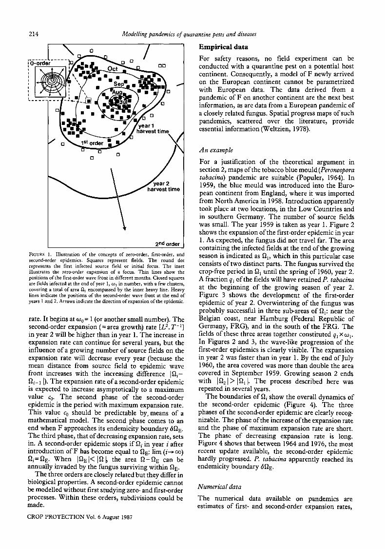
The boundaries of ~i show the overall dynamics of the second-order epidemic (Figure 4). The three phases of the second-order epidemic are clearly recog- nizable. The phase of the increase of the expansion rate and the phase of maximum expansion rate are short. The phase of decreasing expansion rate is long. Figure 4 shows that between 1964 and 1976, the most recent update available, the second-order epidemic hardly progressed. P. tabacina apparently reached its endemicity boundary 6~E.

Numerical data

The numerical data available on pandemics are estimates of first- and second-order expansion rates,

J. A. P. HEESTERBEEK AND J. C. ZADOKS 215

0 400 km I I !

Ju159

f/1

59

- / _ j

FIGURE 2. Expansion ofPeronospora tabacina in 1958 and 1959 (after Populer, 1964, modified). The area covered by the end of 1959 is indicated as I21.

calculated from disease progress maps. As Figures 3 and 4 suggest, estimates of expansion rates are difficult to obtain, the variation over the years being large. A plot of x/- 1~2 i I against time should yield a straight line during the constant phase of expansion (Figures 6 and 8). The slope of the line is the radial expansion rate, expressed in km year-1 [Z. T -1] (Figures 5, 6 and 8). The method is accurate only if the pandemic has radial symmetry (Figure 7), and, as radial symmetry is unusual, the method is approximative only.

Variation in the rate of expansion

Several factors causing variation in the expansion rate of a disease can be indicated. Epidemics are slowed down by geographic factors such as mountains, large water bodies, deserts, and other large host-free areas. The second-order epidemic of chestnut blight (Endothia parasitica) in the USA was held up by the Appalachian mountains (Beattie and Diller, 1954). Fire blight of pear trees (Erwinia amylovora) was held up for years by the Great Plains and the Rocky Mountains when the epidemic travelled from east to west through the USA (Van der Zwet, 1968). Climato- logical factors such as precipitation and temperature were reported to slow down expansion of southern corn leaf blight (Helminthosporium maydis (Cochlio- bolus heterostrophus); Moore, 1970) and Dutch elm

disease (Ophiostoma ulmi; Jay Stipes and Campana, 1981). For Dutch elm disease, climatological factors on the European continent cause ]~EltO be smaller than ]f~ I. In some areas within f~, notably the high Alps and

parts of Finland, where elms can grow, the fungus cannot survive (Heybroek, 1966).

Pathogens with different dispersal mechanisms often show marked differences in expansion rates (Zadoks and Kampmeijer, 1977). Air-borne pathogens travel faster than insect-borne ones. Transportation of propagules by birds can greatly accelerate epidemic expansion. Different dispersal mechanisms often combine to produce complex behaviour, as can be illustrated by Dutch elm disease. The pathogen is dispersed primarily by scolytid beetles but it can also infect trees by way of root contacts. When scolytid beetles can 'hitchhike' on cars along motorways (F. A. Holmes, personal communication), such a third dispersal mechanism ensuring long-distance dispersal will complicate model construction enormously. In zero-order epidemics daughter foci are a normal phenomenon (Zadoks, 1961). In second-order epidemics they occur too, when wind-borne, bird- borne, or man-borne (e.g. car-borne) inoculum initiates foci ahead of the epidemic front. Figure 3 shows the appearance of a daughter focus on 31 July 1960, in the middle of France, when the front of the epidemic had just passed the Franco-Belgian border. Daughter foci

C R O P P R O T E C T I O N Vol. 6 August 1987

216 Modelling pandemics of quarantine pests and diseases

0 4 0 0 k m I I !

20-7 lS-6/,,,

C~2

%

t

f 31-1 • ' ,~ ' * 15-!

30-~

FIGURE 3. Expansion ofPeronospora tabacina in 1960 (after Populer, 1964, modified). The area covered by the end of 1960 is indicated as ~22. In France and Italy loci can be seen which hastened the expansion of the epidemic.

0 4 0 0 km I | I

6 0

l0 !

I ~3

?6 IQ4'

FIGURE 4. Second-order expansion of Peronospora tabacina in Europe, 1959 to 1976 (modified after Populer, 1964, and Commonwealth Mycological Institute, 1976). ~2 i and ~2 E are indicated. The broken lines indicate intermediate late winter situations.

160-

14.0-

120-

100-

80-

60-

4.0-

20-


o j °

o/ / //

I I I I I

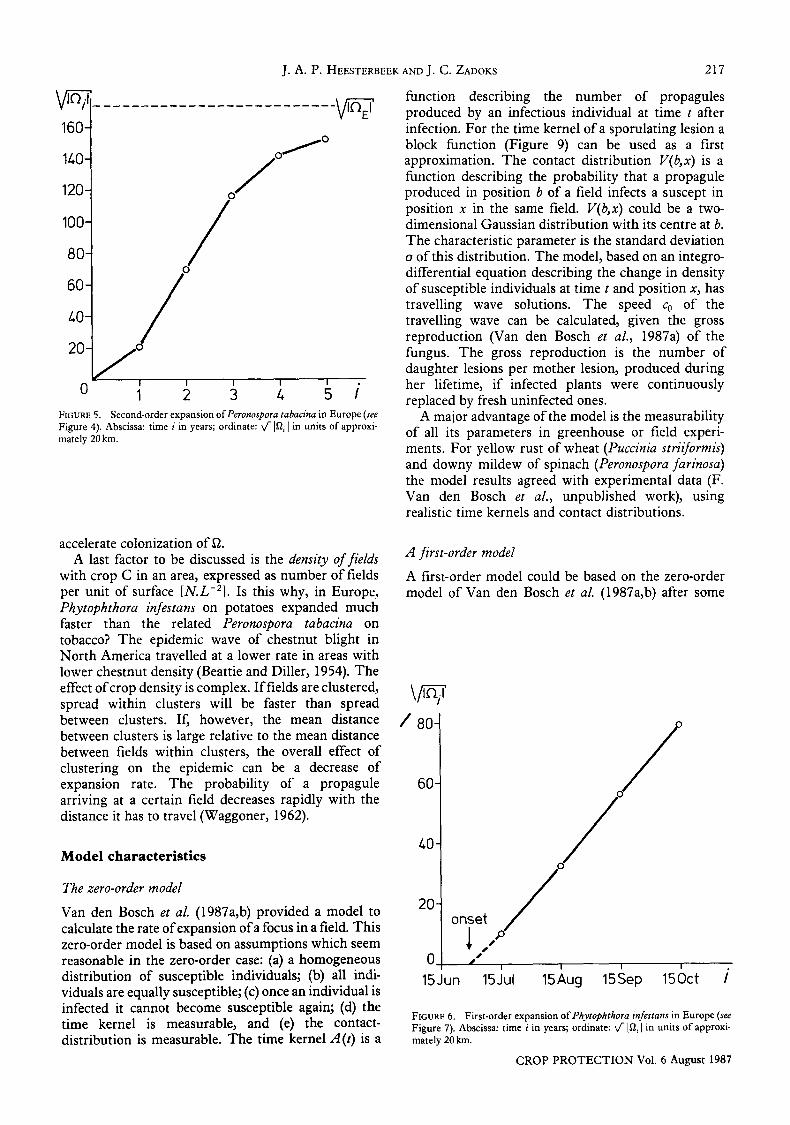
0 1 2 3 4. 5 i FIGURE 5. Second-order expansion ofPeronospora tabacina in Europe (see Figure 4). Abscissa: time i in years; ordinate: ~-]I2 i [in units of approximately 20 km.

function describing the number of propagules produced by an infectious individual at time t after infection. For the time kernel of a sporulating lesion a block function (Figure 9) can be used as a first approximation. The contact distribution V(b,x) is a function describing the probability that a propagule produced in position b of a field infects a suscept in position x in the same field. V(b,x) could be a two- dimensional Gaussian distribution with its centre at b. The characteristic parameter is the standard deviation o of this distribution. The model, based on an integro- differential equation describing the change in density of susceptible individuals at time t and position x, has travelling wave solutions. The speed Co of the travelling wave can be calculated, given the gross reproduction (Van den Bosch et al., 1987a) of the fungus. The gross reproduction is the number of daughter lesions per mother lesion, produced during her lifetime, if infected plants were continuously replaced by fresh uninfected ones.

A major advantage of the model is the measurability of all its parameters in greenhouse or field experi- ments. For yellow rust of wheat (Puccinia striiformis) and downy mildew of spinach (Peronospora farinosa) the model results agreed with experimental data (F. Van den Bosch et al., unpublished work), using realistic time kernels and contact distributions.

accelerate colonization of £. A last factor to be discussed is the density of fields

with crop C in an area, expressed as number of fields per unit of surface IN.L-2]. Is this why, in Europe, Phytophthora infestans on potatoes expanded much faster than the related Peronospora tabacina on tobacco? The epidemic wave of chestnut blight in North America travelled at a lower rate in areas with lower chestnut density (Beattie and Diller, 1954). The effect of crop density is complex. I f fields are clustered, spread within clusters will be faster than spread between clusters. If, however, the mean distance between clusters is large relative to the mean distance between fields within clusters, the overall effect of clustering on the epidemic can be a decrease of expansion rate. The probability of a propagule arriving at a certain field decreases rapidly with the distance it has to travel (Waggoner, 1962).

Model characteristics

The zero-order model

Van den Bosch et al. (1987a,b) provided a model to calculate the rate of expansion of a focus in a field. This zero-order model is based on assumptions which seem reasonable in the zero-order case: (a) a homogeneous distribution of susceptible individuals; (b) all individuals are equally susceptible; (c) once an individual is infected it cannot become susceptible again; (d) the time kernel is measurable, and (e) the contact- distribution is measurable. The time kernel A (t) is a

A first-order model

A first-order model could be based on the zero-order model of Van den Bosch et al. (1987a, b) after some

/ 8o-

60-

40-

20"

0 15Jun

onset

1, J J

J i

15Jul

/// i i i

15Aug 15Sep 150ct

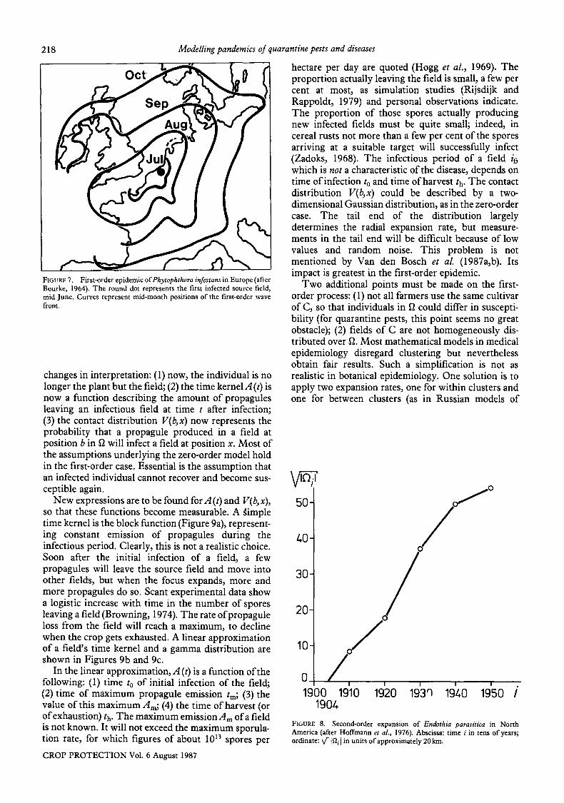
FIGURE 6. First-order expansion ofPhytophthora infestans in Europe (see Figure 7). Abscissa: time i in years; ordinate: X/- If/i I in units of approximately 20 km.

C R O P P R O T E C T I O N Vol. 6 Augus t 1987

218

FIGURE 7. First-order epidemic ofPhytophthora infestans in Europe (after Bourke, 1964). The round dot represents the first infected source field, mid June. Curves represent mid-month positions of the first-order wave front.

changes in interpretation: (1) now, the individual is no longer the plant but the field; (2) the time kernel A (t) is now a function describing the amount of propagules leaving an infectious field at time t after infection; (3) the contact distribution V(b,x) now represents the probability that a propagule produced in a field at position b in ~2 will infect a field at position x. Most of the assumptions underlying the zero-order model hold in the first-order case. Essential is the assumption that an infected individual cannot recover and become susceptible again.

New expressions are to be found for,4 (t) and V(b,x), so that these functions become measurable. A ~imple time kernel is the block function (Figure 9a), represent- ing constant emission of propagules during the infectious period. Clearly, this is not a realistic choice. Soon after the initial infection of a field, a few propagules will leave the source field and move into other fields, but when the focus expands, more and more propagules do so. Scant experimental data show a logistic increase with time in the number of spores leaving a field (Browning, 1974). The rate ofpropagule loss from the field will reach a maximum, to decline when the crop gets exhausted. A linear approximation of a field's time kernel and a gamma distribution are shown in Figures 9b and 9c.

In the linear approximation, ,4 (t) is a function of the following: (1) time to of initial infection of the field; (2) time of maximum propagule emission tin; (3)the value of this maximum Am; (4) the time of harvest (or of exhaustion) th. The maximum emission`4m of a field is not known. It will not exceed the maximum sporulation rate, for which figures of about 1013 spores per

C R O P P R O T E C T I O N Vol. 6 August 1987


hectare per day are quoted (Hogg et al., 1969). The proportion actually leaving the field is small, a few per cent at most, as simulation studies (Rijsdijk and Rappoldt, 1979) and personal observations indicate. The proportion of those spores actually producing new infected fields must be quite small; indeed, in cereal rusts not more than a few per cent of the spores arriving at a suitable target will successfully infect (Zadoks, 1968). The infectious period of a field if, which is not a characteristic of the disease, depends on time of infection to and time of harvest th. The contact distribution V(b,x) could be described by a two- dimensional Gaussian distribution, as in the zero-order case. The tail end of the distribution largely determines the radial expansion rate, but measure- ments in the tail end will be difficult because of low values and random noise. This problem is not mentioned by Van den Bosch et al. (1987a, b). Its impact is greatest in the first-order epidemic.

Two additional points must be made on the first- order process: (1) not all farmers use the same cultivar of C, so that individuals in ~2 could differ in suscepti- bility (for quarantine pests, this point seems no great obstacle); (2) fields of C are not homogeneously distributed over ~2. Most mathematical models in medical epidemiology disregard clustering but nevertheless obtain fair results. Such a simplification is not as realistic in botanical epidemiology. One solution is to apply two expansion rates, one for within clusters and one for between clusters (as in Russian models of

W7 50"

40-

30-

20-

10-

0 1900 1910 /

1904

~ O

I I I I I

1920 193q 1940 1950

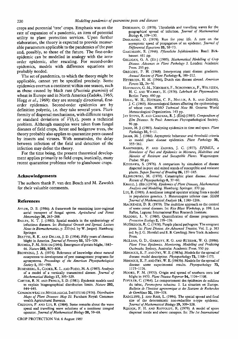
FIGURE 8. Second-order expansion of Endothia parasitica in North America (after Hoffmann et al., 1976). Abscissa: time i in tens of years; ordinate: x/- {~2i] in units of approximately 20 km.

At

J. A. P. HEESTERBEEK AND

block function a

to to . P=te to+P+i f = t h

At

At

to

-Am

-Am

linear function b

to &

gamma function C

to to & FIGURE 9. Time kernels with various degrees of realism. (a) Block function; (b) linear function; (c) gamma function (Van den Bosch et al., 1987a). p=latency period; /=infectious period; t=time; t0=time of infection of the field; t a = time of first sporulation of the field; t m = time of maximum infectiousness of the field; Am=maximum number of propagules leaving the field; t h = harvest time; t h - t a = if= infectious period of the field.

influenza epidemics; Bailey, 1980). The assumption that clusters are homogeneously distributed over £ is not totally unrealistic, as the case of tobacco blue mould shows (Populer, 1964). Then, the first-order model could consist of two steps, one for fields as individuals within clusters and one for clusters as individuals within £.

.

On second-order epidemics

In the case of a second-order epidemic, the analogy with a medical epidemic no longer holds. The zero- order approach cannot be applied because the assumption, that individuals once infected cannot become susceptible again, is no longer valid. Infected fields in year i are replaced by fields, infected or healthy, in year i+ 1. To illustrate some problems in modelling a second-order epidemic, a few important differences between medical and botanical epidemics are mentioned below.

.

J. C. ZADOKS 219

all these processes can be regarded as continuous. In other words: at every time interval, a fraction of the population is born, is infected, dies, recovers, or loses immunity. In the botanical situation things are different. It is still true that farmer A's maize field can be diseased, while his neighbour's field is healthy, and a third field is infected but not yet infectious: the infection process of fields is continuous. However, simultaneity of a maize harvest by farmer A and maize sowing by neighbour B is next to impossible. Within a certain area with crop C, sowing as well as harvesting operations are more or less synchronized. 'Birth' and 'death' of fields are discontinuous processes. The interweaving of discrete and continuous processes in the second- order epidemic has major consequences for model making. In infectious diseases of man, the dispersal of the pathogen is often due to infectious persons moving around. Their movement can be described by a diffusion term. In infectious diseases of plants, fields stay put and the pathogen moves or is moved. This difference affects the way dispersal is treated mathematically. In the medical case, a diffusion term can be added to the differential equation to account for the change in the numbers of susceptible and infectious individuals. In the botanical case, the diffusion term can be applied to the propagules being dispersed. Plant disease epidemics are strongly affected by the 'crop-free period' (Zadoks, 1961) between successive growing seasons, during which practically no spread of disease occurs. Fields can be said to be ' immune' during the crop-free period. In medical epidemics, seasonal effects can be observed, but a 'man-free' period does not exist.

The foregoing analysis indicates that an analytical model of a second-order epidemic is difficult to obtain. Discrete models, with difference equations taking leaps of one year instead of differential equations taking infinitesimally small time steps, may be promising. The useful implication is that empirical data can be limited to an annual assessment of COl at harvest time. Most of the information available about spatial models with discrete time comes from population genetics (Weinberger, 1982; Lui, 1985). These models allow for travelling wave solutions by which the speed of the wave can be calculated (Creegan and Lui, 1984). An alternative is to model the epidemics within the growing seasons by differential equations and between the growing seasons by difference equations, and to couple these models. The dynamic behaviour of such coupled models is as yet unknown.

1. In the medical situation, a patient can become infected by propagules coming from another person. The patient can recover or die while, simultaneously and independently, other people are born or lose immunity. At the population level,

Discuss ion

This paper attempted a theoretical approach to pandemics. The analysis was limited to quarantine diseases which cause polyetic epidemics in annual field

C R O P P R O T E C T I O N Vol. 6 A u g u s t 1987

22O

crops and perennial 'tree' crops. Emphasis was on the rate of expansion of a pandemic, an item of potential utility to plant protection services. Upon further elaboration, the theory is expected to provide measurable parameters applicable to the pandemics of the past and, possibly, to those of the future. The first-order epidemic can be modelled in analogy with the zero- order epidemic, after rescaling. For second-order epidemics, models with difference equations are probably needed.

The set of pandemics, to which the theory might be applicable, cannot yet be specified precisely. Some epidemics overrun a continent within one season, such as those caused by black rust (Puccinia graminis) of wheat in Europe and in North America (Zadoks, 1965; Hogg et al., 1969): they are strongly directional, first- order epidemics. Second-order epidemics are by definition polyetic, i.e. they take several years. Pluri- formity of dispersal mechanisms, with different ranges or standard deviations of V(b,x), poses a technical problem. Although examples were taken from fungal diseases of field crops, forest and hedgerow trees, the theory probably also applies to quarantine pests caused by insects and viruses. With nematodes, the delay between infection of the field and detection of the infection may defeat the theory.

For the time being, the present theoretical development applies primarily to field crops; ironically, many recent quarantine problems refer to glasshouse crops.

Acknowledgements

The authors thank F. van den Bosch and M. Zawolek for their valuable comments.

References

AYLOR, D. E. (1986). A framework for examining inter-regional aerial transport of fungal spores. Agricultural and Forest Meteorology 38, 263-288.

BAILEY, N. T. J. (1980). Spatial models in the epidemiology of infectious diseases. In: Biological Growth and Spread. Lecture Notes in Biomathematics, p. 233 (ed. by W. Jaeger). Hamburg: Springer.

BEATTIE, R. K. AND DILLER, J. D. (1954). Fifty years ofchestuut blight in America. Journal of Forestry 52, 323-329.

BOURKE, P. M. AUSTIN (1964). Emergence of potato blight, 1843- 46. Nature 2113, 805-808.

BROWNING, J. A. (1974). Relevance of knowledge about natural ecosystems to development of pest management programs for agrosystems. Proceedings of the American Phytopathological Society 1, 191-199.

BUSENBERG, S., COOKE, K. L. AND POZlO, M. A. (1983). Analysis of a model of a vertically transmitted disease. Journal of Mathematical Biology 17, 305-329.

CARTER, R. N. AND PRINCE, S. D. (1981). Epidemic models used to explain biogeographical distribution limits. Nature 293, 644-645.

COMMONWEALTH MYCOLOGICAL INSTITUTE (1976). Distribution Maps of Plant Diseases: Map 23. Farnham Royal: Common- wealth Agricultural Bureaux.

CREEGAN, P. AND LUI, R. (1984). Some remarks about the wave speed and travelling wave solutions of a nonlinear integral operator. Journal of Mathematical Biology 20, 59--68.


DIEKMANN, O. (1978). Thresholds and travelling waves for the geographical spread of infection. Journal of Mathematical Biology 6, 109-130.

DIEKMANN, O. (1979). Run for your life. A note on the asymptotic speed of propagation of an epidemic. Journal of Differential Equations 33, 58-73.

GAEUMANN, E. (1946). Pflanzliche Infektionslehre. Basel: Birk- hauser. 611 pp.

GILLIGAN, G. A. (ED.) (1985). Mathematical Modelling of Crop Disease. Advances in Plant Pathology 3. London: Academic Press. 255 pp.

GREGORY, P. H. (1968). Interpreting plant disease gradients. Annual Review of Plant Pathology 6, 189-212.

HEYBROEK, H. M. (1966), Dutch elm disease abroad. American Forests 72, 26-30.

HOFFMANN, G. M., NIENHAUS, F., SCHOENBECK, F., WELTZIEN, H. C. AND WILBERT, H. (1976). Lehrbuch der Phytomedizin. Berlin: Parey. 490 pp.

HOGG, W. H., HOUNAM, C. E., MALLIK, A. K. AND ZADOKS, J. C. (1969). Meteorological factors affecting the epidemiology of wheat rusts. WMO Technical Note 99. Geneva: World Meteorological Organization. 143 pp.

JAY STIPES, R. AND CAMPANA, R. J. (EDS) (1981). Compendium of Elm Diseases. St Paul: American Phytopathological Society. 96 pp.

JEGER, M. J. (1983). Analysing epidemics in time and space. Plant Pathology 32, 5-11.

JEGER, M. J. (1986). Asymptotic behaviour and threshold criteria in model plant disease epidemics. Plant Pathology 35, 355-361.

KAMPMEIJER, P. AND ZADOKS, J. C. (1977). EPIMUL, a Simulator of Foci and Epidemics in Mixtures, Multilines and Mosaics of Resistant and Susceptible Plants. Wageningen: Pudoc. 50 pp.

KIYOSAWA, S. (1976). A comparison by simulation of disease dispersal in pure and mixed stands of susceptible and resistant plants. Japan Journal of Breeding 2t;, 137-145.

KLINKOWSKI, M. (1970). Catastrophic plant disease. Annual Review of Phytopathology 8, 37-60.

KRANZ, J. (ED.)(1974). Epidemics of Plant Diseases, Mathematical Analysis and Modelling. Hamburg: Springer. 170 pp.

LuI, R. (1985). A nonlinear integral operator arising from a model in population genetics. 3. Heterozygote inferior case. SIAM Journal of Mathematical Analysis 16, 1180-1206.

MACKENZIE, D. R. (1979). The multiline approach to the control of some cereal diseases. In: Rice Blast Workshop, p. 199. Los Baffos, Laguna: International Rice Research Institute.

MADDEN, L. V. (1980). Quantification of disease progression. Protection Ecology 2, 159-176.

McGREGOR, R. C. (1978). People placed pathogens: The emigrant pests. In: Plant Disease. An Advanced Treatise, Vol. 2, p. 383 (ed. by J. G. Horsfall and E. B. Cowling). New York: Academic Press.

MCLEAN, G. D., GARRETT, R. G. AND RUESINK, W. G. (1986). Plant Virus Epidemics. Monitoring, Modelling and Predicting Outbreaks. Sydney, Australia: Academic Press. 550 pp.

MINOGUE, K. P. AND FRY, W. E. (1983a). Models for the spread of disease: model description. Phytopathology 73, 1168-1173.

MINOGUE, K. P. AND FRY, W. E. (1983b). Models for the spread of disease: some experimental results. Phytopathology 7:1, 1173-1176.

MOORE, F. M. (1970). Origin and spread of southern corn leaf blight in 1970. Plant Disease Reporter 54, 1104-1108.

POPULER, C. (1964). Le comportement des 6pid6mies de mildiou du tabac, Peronospora tabacina. 1. La situation en Europe. Bulletin de l'Institut agronomique et des Stations de Recherches de Gembloux 32, 339-378.

RADCLIFFE, J. AND RASS, L. (1984). The spatial spread and final size of the deterministic non-reducible n-type epidemic. Journal of Mathematical Biology 19, 309-328.

RIJSDIJK, F. H. AND RAPPOLDT, K. (1979). A model of spore dispersal inside and above canopies. In: The 1st International



Conference on Aerobiology: Federal Environmental Agency, p. 407. Berlin: Erich Schmidt.

SCHEPEgS, H. T. A. M. (1984). A pattern in the appearance of cucumber mildew in Dutch glasshouses. NetherlandsJournalof Plant Pathology 90, 247-256.

SCHROEDTER, H. (1960). Dispersal by air and water--the flight and landing. In: Plant Pathology, An Advanced Treatise, Vol. 3, p. 169 (ed. by J. G. Horsfall and A. E. Dimond). New York: Academic Press.

SKELLAM, J. G. (1951). Random dispersal in theoretical populations. Biometrika 38, 196-218.

TENG, P. S. (1985). A comparison of simulation approaches to epidemic modelling. Annual Review of Phytopathology 23, 351-379.

THIEME, H. R. (1977). A model for the spatial spread of an epidemic. Journal of Mathematical Biology 4, 337-351.

VAN DEN BOSCH, F., METZ, J. A. J. AND ZADOKS, J. C. (1987a). Focus formation in plant disease. I. The constant rate of focus expansion. Phytopathology 77, in press.

VAN DEN BOSCH, F., METZ, J. A. J. AND ZADOKS, J. C. (1987b). Focus formation in plant disease. II. Realistic parameter-sparse models. Phytopathology 77, in press.

VAN DER PLANK, J. E. (1963). Plant Diseases, Epidemics and Control. New York: Academic Press. 350 pp.

VAN DER ZWET, T. (1968). Recent spread and present distribution of fire blight in the world. Plant Disease Reporter 52, 698-702.

WAGGONER, P. E. (1962). Weather, space, time, and chance of infection. Phytopathology 52, 1100--1108.

WEINBERGER, H. F. (1982). Long-time behaviour of a class ofbio-

logical models. SlAM Journal of Mathematical Analysis 13, 353-396.

WELTZIEN, H. C. (1978). Geophytopathology. In: Plant Pathology, An Advanced Treatis~ Vol. 2, p. 339 (ed. by J. G. Horsfall and A. E. Dimond). New York: Academic Press.

ZADOKS, J. C. (1961). Yellow rust on wheat, studies in epidemiology and physiologic specialisation. Tijdschrift over Planteziekten 67, 69-256.

ZADOKS, J. C. (1965). Epidemiology of wheat rusts in Europe. FAO Plant Protection Bulletin 13, 97-108.

ZADOKS, J. C. (1968). Meteorological factors involved in the dispersal of cereal rusts. In: Proceedings of a Regional Training Seminar on Agrometeorology, p. 179 (ed. by A. J. W. Borghorst). Wageningen.

ZADOKS, J. C. (1979). Simulation of epidemics: problems and applications. EPPO Bulletin 9, 227-234.

ZADOKS, J. C. AND KAMPMEIJER, P. (1977). The role of crop populations and their deployment illustrated by means of a simulator EPIMUL76. Annals of the New York Academy of Sciences 287, 164-190.

ZADOKS, J. C. AND SCHEIN, R. D. (1979). Epidemiology and Plant Disease Management. New York: Oxford University Press. 427 pp.

Received 27 July 1986 Revised 19 January 1987 Accepted 2 February 1987


Documents

Modelling pandemics of quarantine pests and diseases: problems