IB HL MATHS PORTFOLIO TYPE II

Modelling Probabilities in

Games of Tennis

Tousif Ahmed

IBDP1, Oaktree International School

Abstract

“What men want is not knowledge, but certainty.” - Bertrand Russell (1872-1970)

Probability is a subject which deals mostly with certainty and gives us the impression of

something that is bound to happen or not to happen or happen in a specific manner. Yet, it

cannot tell us the absolute truth of any occurrence; since the occurrence is not governed by

probability itself. Though, through probability one might not find the absolute certainty; but at

least he can get as closer to the absolute certainty. Thus, this paper struggles to examine the

probability model for a game of tennis. It analyzes the relationship between a binomial

probability distribution and the process of match play in tennis and constructs a probability

model for two players of predictable abilities. It also investigates two models of resolving ties.

2

1 Table of Contents

2 Tennis Scoring .......................................................................................................................... 3

3 Binomial Distribution and Tennis ............................................................................................ 3

3.1 Binomial Distribution Model for a Tennis Club Practice ................................................ 3

3.2 Limitations of a Binomial Distribution Model for Tennis ................................................ 4

3.3 Histogram, Expected Value and Standard Deviation of the Binomial Distribution

Model for Tennis Club Practice ................................................................................................... 5

3.3.1 Method for calculations ........................................................................................ 6

3.4 Analysis of the Expected Value and the Standard Deviation obtained in 2.3 ................. 6

4 Non-extended Play Games ....................................................................................................... 8

4.1 Non-extended Play Games Scoring .................................................................................. 8

4.2 Binomial Distribution Model for Non-extended Play Games .......................................... 9

4.2.1 Probability Model for Adam Winning a Non-extended Play Game ................... 10

4.2.2 Probability Model for Ben Winning a Non-extended Play Game ....................... 11

4.3 Probability and Odds...................................................................................................... 11

4.3.1 Probability of Adam Winning the Non-extended Play Game ............................. 11

4.3.2 Probability of Ben Winning the Non-extended Play Game ................................ 12

4.3.3 Odds of Adam Winning the Game ..................................................................... 12

4.3.4 Odds of Ben Winning the Game ......................................................................... 12

4.4 Probability of winning Non-extended Play Game of Player C ...................................... 12

5 Extended Play Games ............................................................................................................ 12

5.1 Probability of Winning a Non-deuce Game ................................................................... 12

5.1.1 Verification of the formulae ................................................................................ 13

5.1.2 Odds of Adam Winning a Non-deuce Game ....................................................... 13

5.2 Probability of Winning a Deuce Game .......................................................................... 14

5.2.1 Verification of the formulae ................................................................................ 16

5.2.2 Odds of Adam Winning the Deuce Game ........................................................... 16

6 Analysis of the Certainty of Winning a Non-deuce Game and a Deuce Game ..................... 17

7 Usefulness of Probability Models in Tennis ........................................................................... 23

8 Conclusion .............................................................................................................................. 23

3

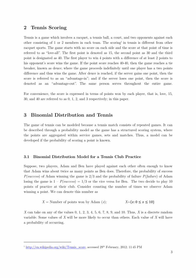
2 Tennis Scoring

Tennis is a game which involves a racquet, a tennis ball, a court, and two opponents against each

other consisting of 1 or 2 members in each team. The scoring1 in tennis is different from other

racquet sports. The game starts with no score on each side and the score at that point of time is

referred to as “love-all”. The first point is denoted as 15, the second point as 30 and the third

point is designated as 40. The first player to win 4 points with a difference of at least 2 points to

his opponent’s score wins the game. If the point score reaches 40-40, then the game reaches a tie

breaker, known as deuce; where the game proceeds indefinitely until one player has a two points

difference and thus wins the game. After deuce is reached, if the server gains one point, then the

score is referred to as an “advantage-in”; and if the server loses one point, then the score is

denoted as an “advantage-out”. The same person serves throughout the entire game.

For convenience, the score is expressed in terms of points won by each player, that is, love, 15,

30, and 40 are referred to as 0, 1, 2, and 3 respectively; in this paper.

3 Binomial Distribution and Tennis

The game of tennis can be modeled because a tennis match consists of repeated games. It can

be described through a probability model as the game has a structured scoring system, where

the points are aggregated within service games, sets and matches. Thus, a model can be

developed if the probability of scoring a point is known.

3.1 Binomial Distribution Model for a Tennis Club Practice

Suppose, two players, Adam and Ben have played against each other often enough to know

that Adam wins about twice as many points as Ben does. Therefore, the probability of success

P(success) of Adam winning the game is 2/3 and the probability of failure P(failure) of Adam

losing the game is 1 – P(success) = 1/3 or the vice versa for Ben. The two decide to play 10

points of practice at their club. Consider counting the number of times we observe Adam

winning a point. We can denote this number as

X = Number of points won by Adam (x); X=��: 0 ≤ � ≤ 10}

X can take on any of the values 0, 1, 2, 3, 4, 5, 6, 7, 8, 9, and 10. Thus, X is a discrete random

variable. Some values of X will be more likely to occur than others. Each value of X will have

a probability of occurring.

1 http://en.wikipedia.org/wiki/Tennis_score, accessed 29th February, 2012; 11:45 PM

4

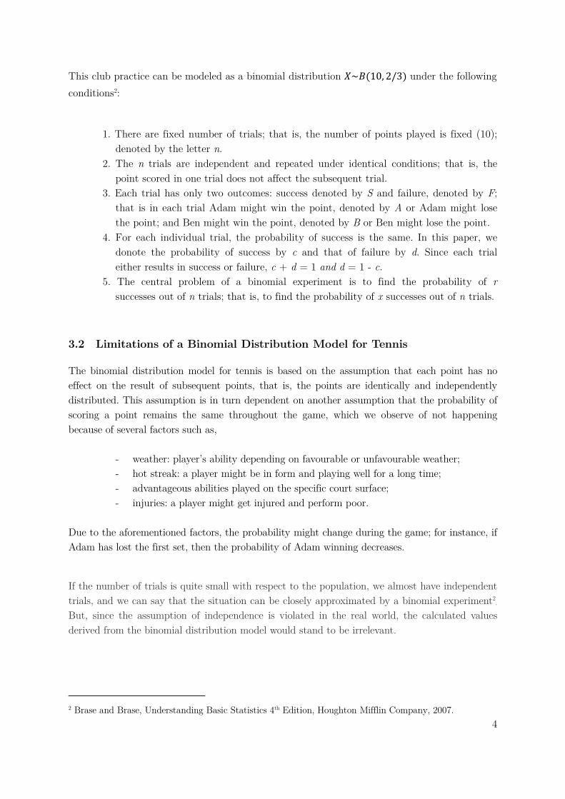
This club practice can be modeled as a binomial distribution �~�(10, 2/3) under the following conditions2:

1. There are fixed number of trials; that is, the number of points played is fixed (10);

denoted by the letter n.

2. The n trials are independent and repeated under identical conditions; that is, the

point scored in one trial does not affect the subsequent trial.

3. Each trial has only two outcomes: success denoted by S and failure, denoted by F;

that is in each trial Adam might win the point, denoted by A or Adam might lose

the point; and Ben might win the point, denoted by B or Ben might lose the point.

4. For each individual trial, the probability of success is the same. In this paper, we

donote the probability of success by c and that of failure by d. Since each trial

either results in success or failure, c + d = 1 and d = 1 - c.

5. The central problem of a binomial experiment is to find the probability of r

successes out of n trials; that is, to find the probability of x successes out of n trials.

3.2 Limitations of a Binomial Distribution Model for Tennis

The binomial distribution model for tennis is based on the assumption that each point has no

effect on the result of subsequent points, that is, the points are identically and independently

distributed. This assumption is in turn dependent on another assumption that the probability of

scoring a point remains the same throughout the game, which we observe of not happening

because of several factors such as,

- weather: player’s ability depending on favourable or unfavourable weather;

- hot streak: a player might be in form and playing well for a long time;

- advantageous abilities played on the specific court surface;

- injuries: a player might get injured and perform poor.

Due to the aforementioned factors, the probability might change during the game; for instance, if

Adam has lost the first set, then the probability of Adam winning decreases.

If the number of trials is quite small with respect to the population, we almost have independent

trials, and we can say that the situation can be closely approximated by a binomial experiment2.

But, since the assumption of independence is violated in the real world, the calculated values

derived from the binomial distribution model would stand to be irrelevant.

2 Brase and Brase, Understanding Basic Statistics 4th Edition, Houghton Mifflin Company, 2007.

5

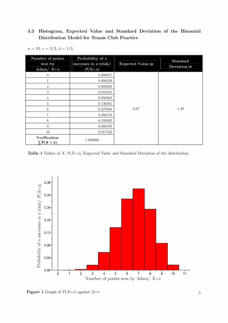
3.3 Histogram, Expected Value and Standard Deviation of the Binomial

Distribution Model for Tennis Club Practice

n = 10, c = 2/3, d = 1/3,

Number of points

won by

Adam/ X=x

Probability of x

successes in n trials/

P(X=x)

Expected Value/� Standard

Deviation/�

0 0.000017

6.67

1.49

1 0.000339

2 0.003048

3 0.016258

4 0.056902

5 0.136565

6 0.227608

7 0.260123

8 0.195092

9 0.086708

10 0.017342

Verification: ∑�(� = �)

1.000000

Table 1 Values of X, P(X=x), Expected Value and Standard Deviation of the distribution

Figure 1 Graph of P(X=x) against X=x

6

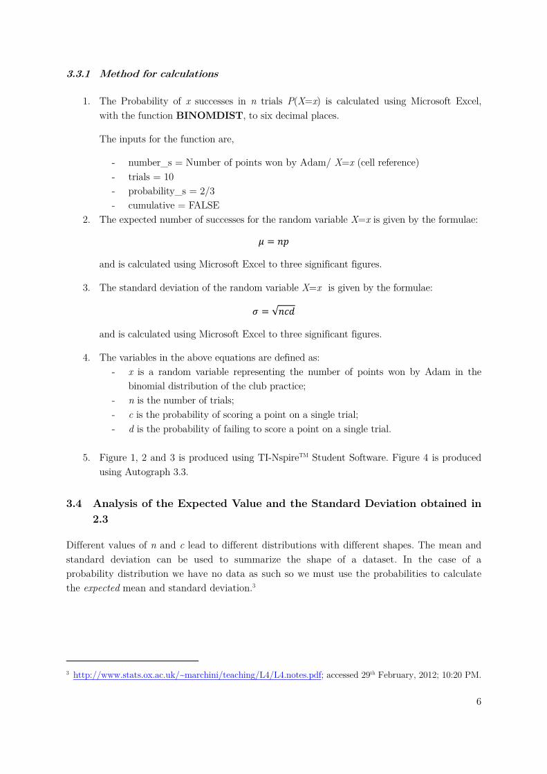
3.3.1 Method for calculations

1. The Probability of x successes in n trials P(X=x) is calculated using Microsoft Excel,

with the function BINOMDIST, to six decimal places.

The inputs for the function are,

- number_s = Number of points won by Adam/ X=x (cell reference)

- trials = 10

- probability_s = 2/3

- cumulative = FALSE

2. The expected number of successes for the random variable X=x is given by the formulae:

� = �� and is calculated using Microsoft Excel to three significant figures.

3. The standard deviation of the random variable X=x is given by the formulae:

� = √�� and is calculated using Microsoft Excel to three significant figures.

4. The variables in the above equations are defined as:

- x is a random variable representing the number of points won by Adam in the

binomial distribution of the club practice;

- n is the number of trials;

- c is the probability of scoring a point on a single trial;

- d is the probability of failing to score a point on a single trial.

5. Figure 1, 2 and 3 is produced using TI-NspireTM Student Software. Figure 4 is produced

using Autograph 3.3.

3.4 Analysis of the Expected Value and the Standard Deviation obtained in

2.3

Different values of n and c lead to different distributions with different shapes. The mean and

standard deviation can be used to summarize the shape of a dataset. In the case of a

probability distribution we have no data as such so we must use the probabilities to calculate

the expected mean and standard deviation.3

3 http://www.stats.ox.ac.uk/~marchini/teaching/L4/L4.notes.pdf; accessed 29th February, 2012; 10:20 PM.

7

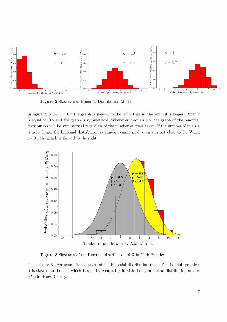
In figure 2, when c = 0.7 the graph is skewed to the left – that is, the left tail is longer. When c

is equal to O.5 and the graph is symmetrical. Whenever c equals 0.5, the graph of the binomial

distribution will be symmetrical regardless of the number of trials taken. If the number of trials n

is quite large, the binomial distribution is almost symmetrical, even c is not close to 0.5 When

c= 0.1 the graph is skewed to the right.

Thus, figure 3, represents the skewness of the binomial distribution model for the club practice.

It is skewed to the left, which is seen by comparing it with the symmetrical distribution at c =

0.5. (In figure 3 c = p)

Figure 2 Skewness of Binomial Distribution Models

Figure 3 Skewness of the Binomial distribution of X in Club Practice

n = 10

c = 0.1

n = 10

c = 0.5

n = 10

c = 0.7

8

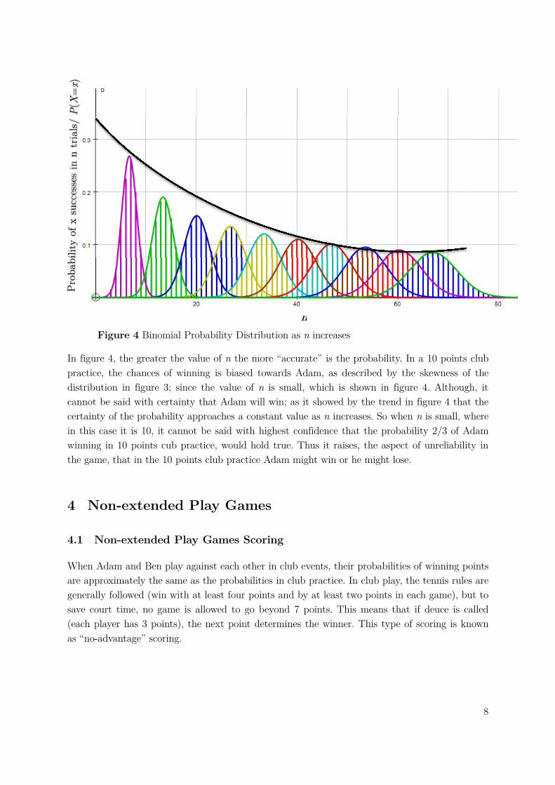
In figure 4, the greater the value of n the more “accurate” is the probability. In a 10 points club

practice, the chances of winning is biased towards Adam, as described by the skewness of the

distribution in figure 3; since the value of n is small, which is shown in figure 4. Although, it

cannot be said with certainty that Adam will win; as it showed by the trend in figure 4 that the

certainty of the probability approaches a constant value as n increases. So when n is small, where

in this case it is 10, it cannot be said with highest confidence that the probability 2/3 of Adam

winning in 10 points cub practice, would hold true. Thus it raises, the aspect of unreliability in

the game, that in the 10 points club practice Adam might win or he might lose.

4 Non-extended Play Games

4.1 Non-extended Play Games Scoring

When Adam and Ben play against each other in club events, their probabilities of winning points

are approximately the same as the probabilities in club practice. In club play, the tennis rules are

generally followed (win with at least four points and by at least two points in each game), but to

save court time, no game is allowed to go beyond 7 points. This means that if deuce is called

(each player has 3 points), the next point determines the winner. This type of scoring is known

as “no-advantage” scoring.

n

Figure 4 Binomial Probability Distribution as n increases

9

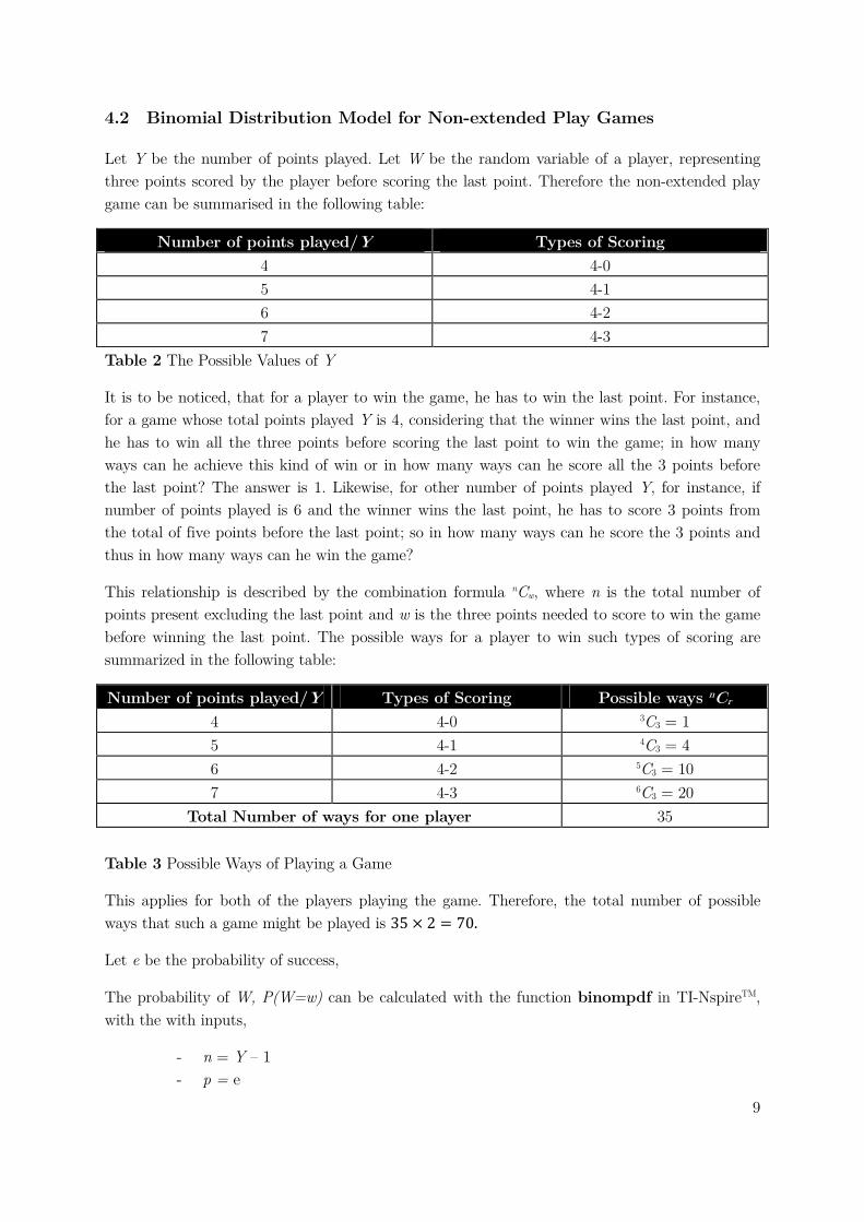
4.2 Binomial Distribution Model for Non-extended Play Games

Let Y be the number of points played. Let W be the random variable of a player, representing

three points scored by the player before scoring the last point. Therefore the non-extended play

game can be summarised in the following table:

Number of points played/Y Types of Scoring

4 4-0

5 4-1

6 4-2

7 4-3

Table 2 The Possible Values of Y

It is to be noticed, that for a player to win the game, he has to win the last point. For instance,

for a game whose total points played Y is 4, considering that the winner wins the last point, and

he has to win all the three points before scoring the last point to win the game; in how many

ways can he achieve this kind of win or in how many ways can he score all the 3 points before

the last point? The answer is 1. Likewise, for other number of points played Y, for instance, if

number of points played is 6 and the winner wins the last point, he has to score 3 points from

the total of five points before the last point; so in how many ways can he score the 3 points and

thus in how many ways can he win the game?

This relationship is described by the combination formula nCw, where n is the total number of

points present excluding the last point and w is the three points needed to score to win the game

before winning the last point. The possible ways for a player to win such types of scoring are

summarized in the following table:

Number of points played/Y Types of Scoring Possible ways nCr

4 4-0 3C3 = 1

5 4-1 4C3 = 4

6 4-2 5C3 = 10

7 4-3 6C3 = 20

Total Number of ways for one player 35

Table 3 Possible Ways of Playing a Game

This applies for both of the players playing the game. Therefore, the total number of possible

ways that such a game might be played is 35 × 2 = 70.

Let e be the probability of success,

The probability of W, P(W=w) can be calculated with the function binompdf in TI-NspireTM,

with the with inputs,

- n = Y – 1

- p = e

10

- X value = 3

Therefore, the probability model for such a game would be:

P(win) = P(4-0) + P(4-1) + P(4-2) + P(4-3)

= e[binompdf(n1,e1,3) + binompdf(n2,e2,3) + binompdf(n3,e3,3) + binompdf(n4,e4,3)]

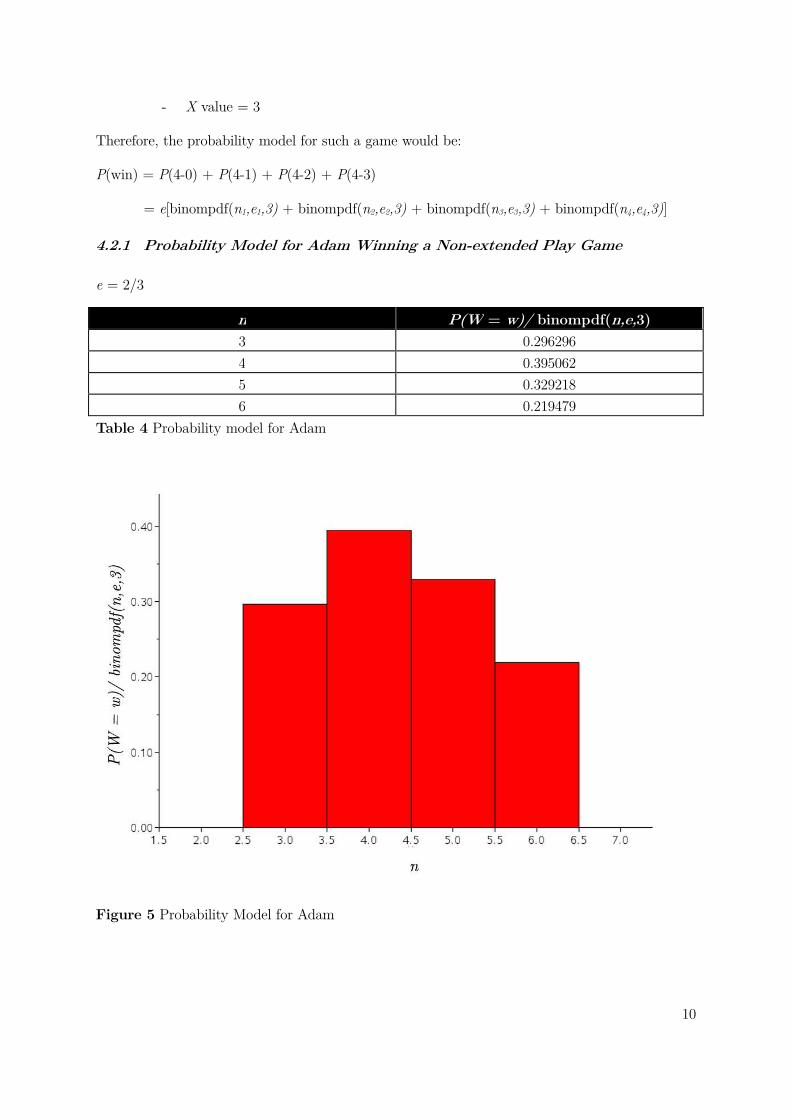
4.2.1 Probability Model for Adam Winning a Non-extended Play Game

e = 2/3

n P(W = w)/ binompdf(n,e,3)

3 0.296296

4 0.395062

5 0.329218

6 0.219479

Table 4 Probability model for Adam

Figure 5 Probability Model for Adam

11

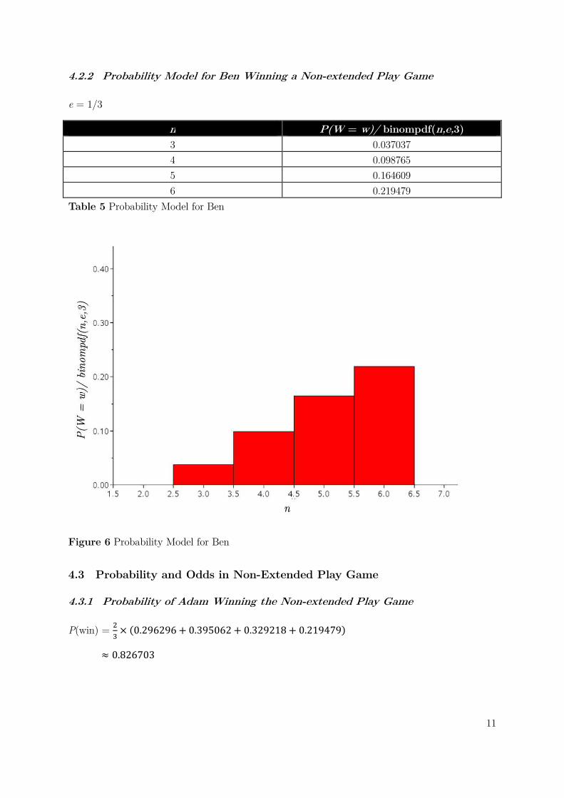
4.2.2 Probability Model for Ben Winning a Non-extended Play Game

e = 1/3

n P(W = w)/ binompdf(n,e,3)

3 0.037037

4 0.098765

5 0.164609

6 0.219479

Table 5 Probability Model for Ben

Figure 6 Probability Model for Ben

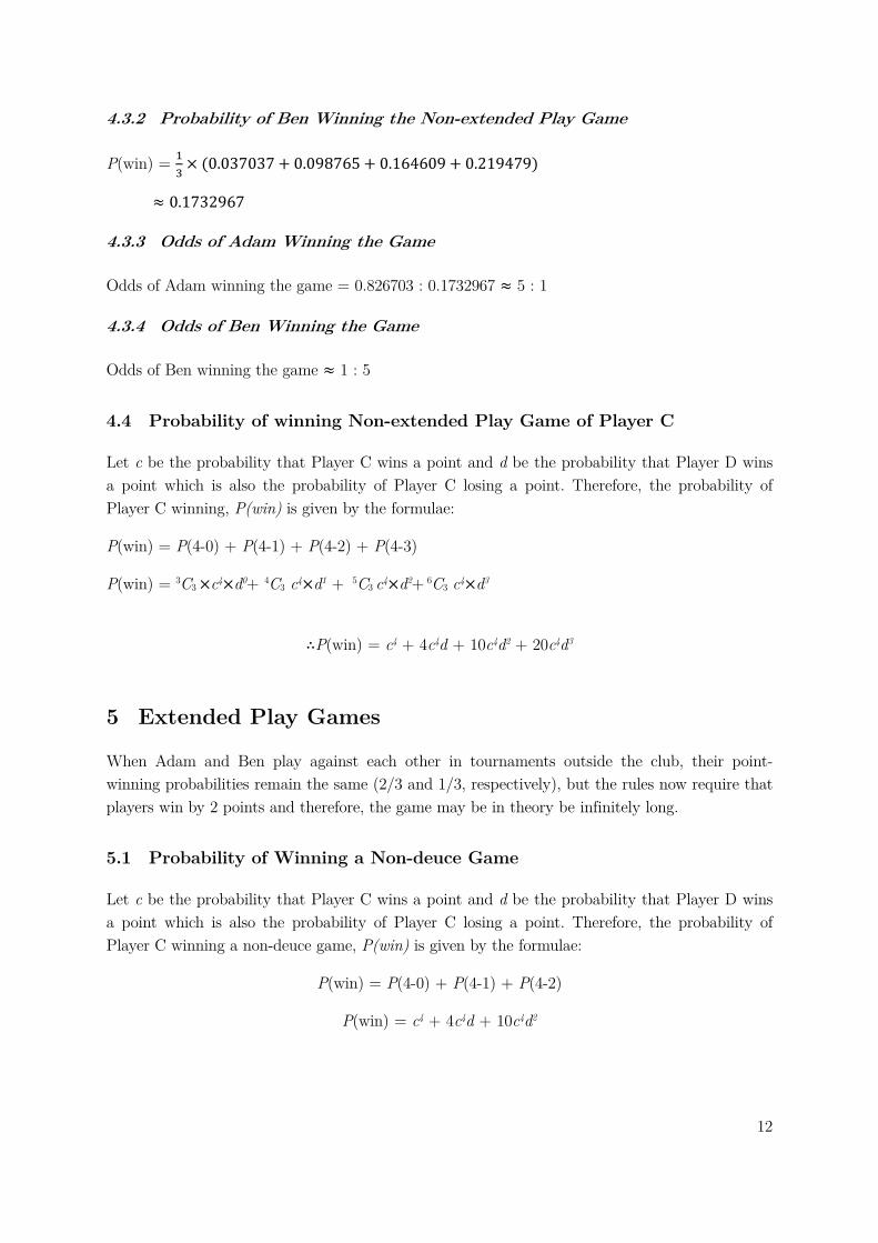
4.3 Probability and Odds in Non-Extended Play Game

4.3.1 Probability of Adam Winning the Non-extended Play Game

P(win) = �� × �0.296296 + 0.395062 + 0.329218 + 0.219479

≈ 0.826703

12

4.3.2 Probability of Ben Winning the Non-extended Play Game

P(win) = �� × (0.037037 + 0.098765 + 0.164609 + 0.219479)

≈ 0.1732967

4.3.3 Odds of Adam Winning the Game

Odds of Adam winning the game = 0.826703 : 0.1732967 ≈ 5 : 1

4.3.4 Odds of Ben Winning the Game

Odds of Ben winning the game ≈ 1 : 5

4.4 Probability of winning Non-extended Play Game of Player C

Let c be the probability that Player C wins a point and d be the probability that Player D wins

a point which is also the probability of Player C losing a point. Therefore, the probability of

Player C winning, P(win) is given by the formulae:

P(win) = P(4-0) + P(4-1) + P(4-2) + P(4-3)

P(win) = 3C3 ×c4×d0+ 4C3 c4×d1 + 5C3 c4×d2+ 6C3 c4×d3

∴P(win) = c4 + 4c4d + 10c4d2 + 20c4d3

5 Extended Play Games

When Adam and Ben play against each other in tournaments outside the club, their point-

winning probabilities remain the same (2/3 and 1/3, respectively), but the rules now require that

players win by 2 points and therefore, the game may be in theory be infinitely long.

5.1 Probability of Winning a Non-deuce Game

Let c be the probability that Player C wins a point and d be the probability that Player D wins

a point which is also the probability of Player C losing a point. Therefore, the probability of

Player C winning a non-deuce game, P(win) is given by the formulae:

P(win) = P(4-0) + P(4-1) + P(4-2)

P(win) = c4 + 4c4d + 10c4d2

13

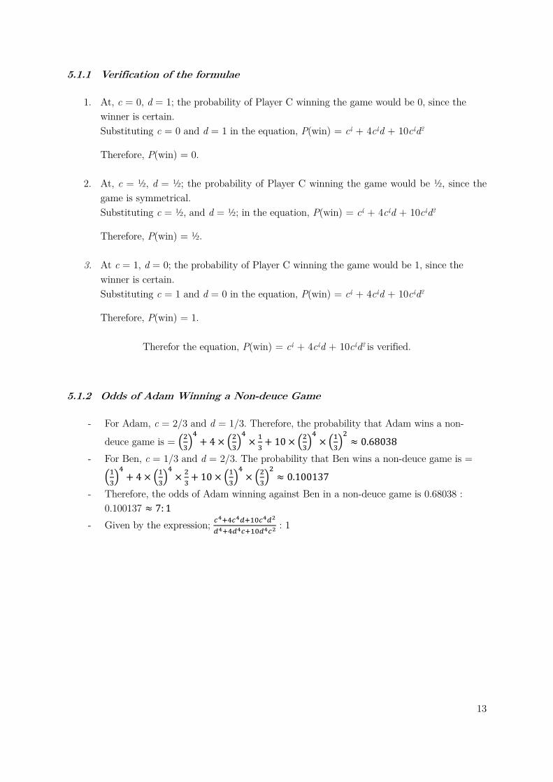
5.1.1 Verification of the formulae

1. At, c = 0, d = 1; the probability of Player C winning the game would be 0, since the

winner is certain.

Substituting c = 0 and d = 1 in the equation, P(win) = c4 + 4c4d + 10c4d2

Therefore, P(win) = 0.

2. At, c = ½, d = ½; the probability of Player C winning the game would be ½, since the

game is symmetrical.

Substituting c = ½, and d = ½; in the equation, P(win) = c4 + 4c4d + 10c4d2

Therefore, P(win) = ½.

3. At c = 1, d = 0; the probability of Player C winning the game would be 1, since the

winner is certain.

Substituting c = 1 and d = 0 in the equation, P(win) = c4 + 4c4d + 10c4d2

Therefore, P(win) = 1.

Therefor the equation, P(win) = c4 + 4c4d + 10c4d2 is verified.

5.1.2 Odds of Adam Winning a Non-deuce Game

- For Adam, c = 2/3 and d = 1/3. Therefore, the probability that Adam wins a non-

deuce game is = ����� + 4 × ����� × �� + 10 × ����� × ����� ≈ 0.68038

- For Ben, c = 1/3 and d = 2/3. The probability that Ben wins a non-deuce game is =

����� + 4 × ����� × �� + 10 × ����� × ����� ≈ 0.100137

- Therefore, the odds of Adam winning against Ben in a non-deuce game is 0.68038 :

0.100137 ≈ 7: 1

- Given by the expression; ��������������

�������������� : 1

14

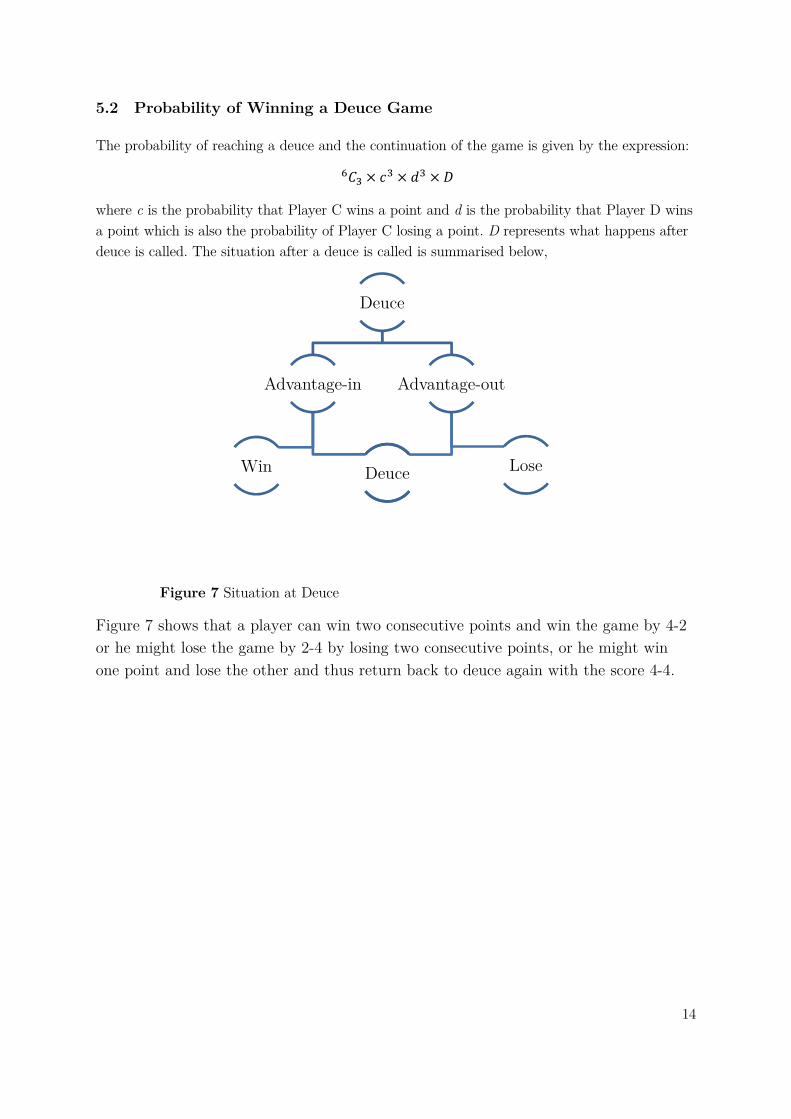
5.2 Probability of Winning a Deuce Game

The probability of reaching a deuce and the continuation of the game is given by the expression:

�� × � × �� × �

where c is the probability that Player C wins a point and d is the probability that Player D wins

a point which is also the probability of Player C losing a point. D represents what happens after

deuce is called. The situation after a deuce is called is summarised below,

Figure 7 shows that a player can win two consecutive points and win the game by 4-2

or he might lose the game by 2-4 by losing two consecutive points, or he might win

one point and lose the other and thus return back to deuce again with the score 4-4.

Deuce

Advantage-in

DeuceWin

Advantage-out

Lose

Figure 7 Situation at Deuce

15

Deuce

Advantage-in

DeuceWin

Advantage-out

LoseDeuce

Advantage-in

DeuceWin

Advantage-out

Lose

Deuce

Advantage-in

DeuceWin

Advantage-out

Lose

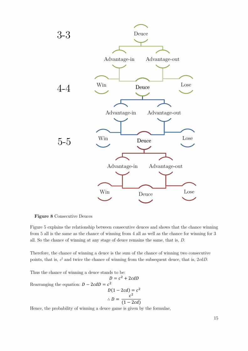
Figure 5 explains the relationship between consecutive deuces and shows that the chance winning

from 5 all is the same as the chance of winning from 4 all as well as the chance for winning for 3

all. So the chance of winning at any stage of deuce remains the same, that is, D.

Therefore, the chance of winning a deuce is the sum of the chance of winning two consecutive

points, that is, c2 and twice the chance of winning from the subsequent deuce, that is, 2cdD.

Thus the chance of winning a deuce stands to be: � = � + 2�� Rearranging the equation: � − 2�� = � ��1 − 2� = �

∴ � = �(1 − 2�)

Hence, the probability of winning a deuce game is given by the formulae,

3-3

4-4

5-5

Figure 8 Consecutive Deuces

16

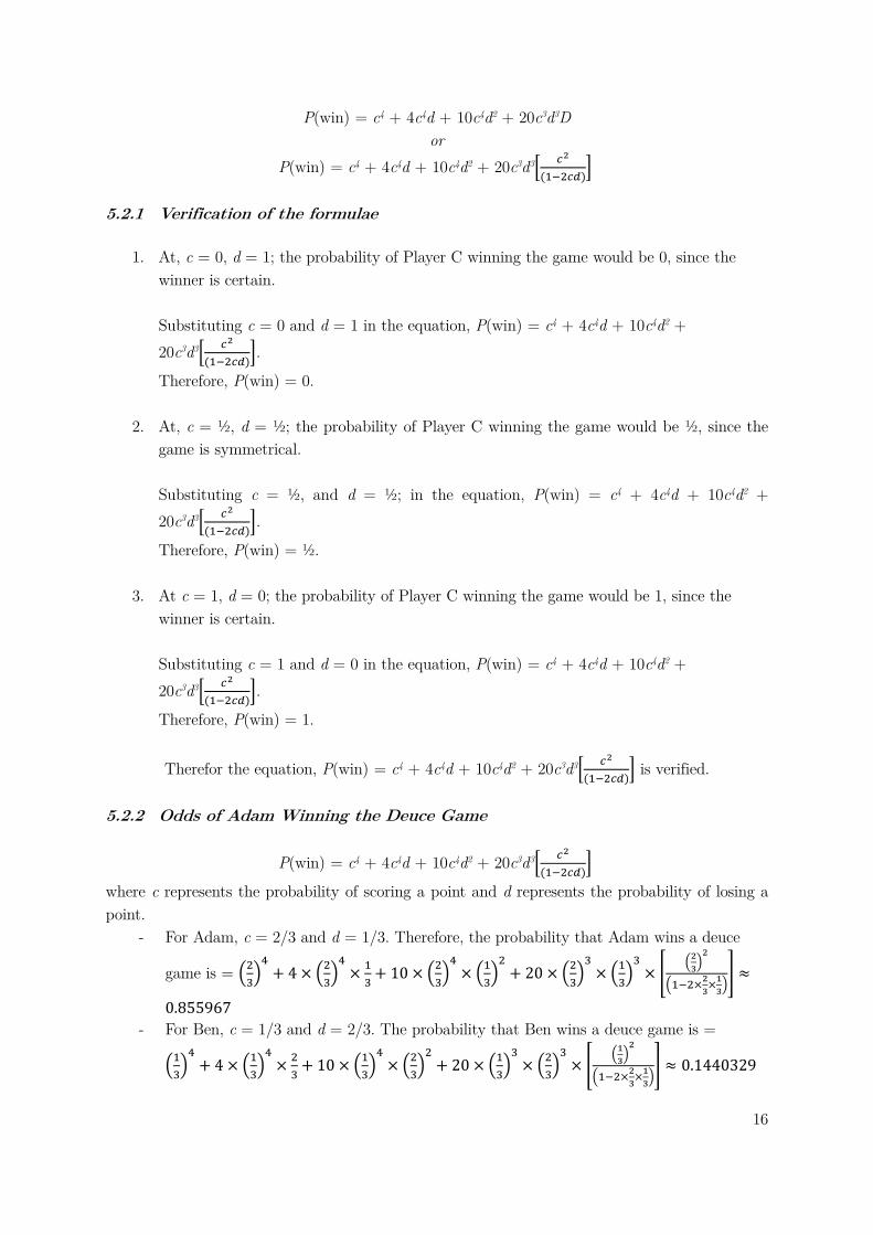
P(win) = c4 + 4c4d + 10c4d2 + 20c3d3D

or

P(win) = c4 + 4c4d + 10c4d2 + 20c3d3� ��(����)�

5.2.1 Verification of the formulae

1. At, c = 0, d = 1; the probability of Player C winning the game would be 0, since the

winner is certain.

Substituting c = 0 and d = 1 in the equation, P(win) = c4 + 4c4d + 10c4d2 +

20c3d3� ��(����)�.

Therefore, P(win) = 0.

2. At, c = ½, d = ½; the probability of Player C winning the game would be ½, since the

game is symmetrical.

Substituting c = ½, and d = ½; in the equation, P(win) = c4 + 4c4d + 10c4d2 +

20c3d3� ��(����)�.

Therefore, P(win) = ½.

3. At c = 1, d = 0; the probability of Player C winning the game would be 1, since the

winner is certain.

Substituting c = 1 and d = 0 in the equation, P(win) = c4 + 4c4d + 10c4d2 +

20c3d3� ��(����)�.

Therefore, P(win) = 1.

Therefor the equation, P(win) = c4 + 4c4d + 10c4d2 + 20c3d3� ��(����)� is verified.

5.2.2 Odds of Adam Winning the Deuce Game

P(win) = c4 + 4c4d + 10c4d2 + 20c3d3� ��(����)�

where c represents the probability of scoring a point and d represents the probability of losing a

point.

- For Adam, c = 2/3 and d = 1/3. Therefore, the probability that Adam wins a deuce

game is = ����� + 4 × ����� × ��+ 10 × ����� × ����� + 20 × ����� × ����� × � ��

���

����

��

��� ≈

0.855967

- For Ben, c = 1/3 and d = 2/3. The probability that Ben wins a deuce game is =

����� + 4 × ����� × �� + 10 × ����� × ����� + 20 × ����� × ����� × � ��

���

����

��

��� ≈ 0.1440329

17

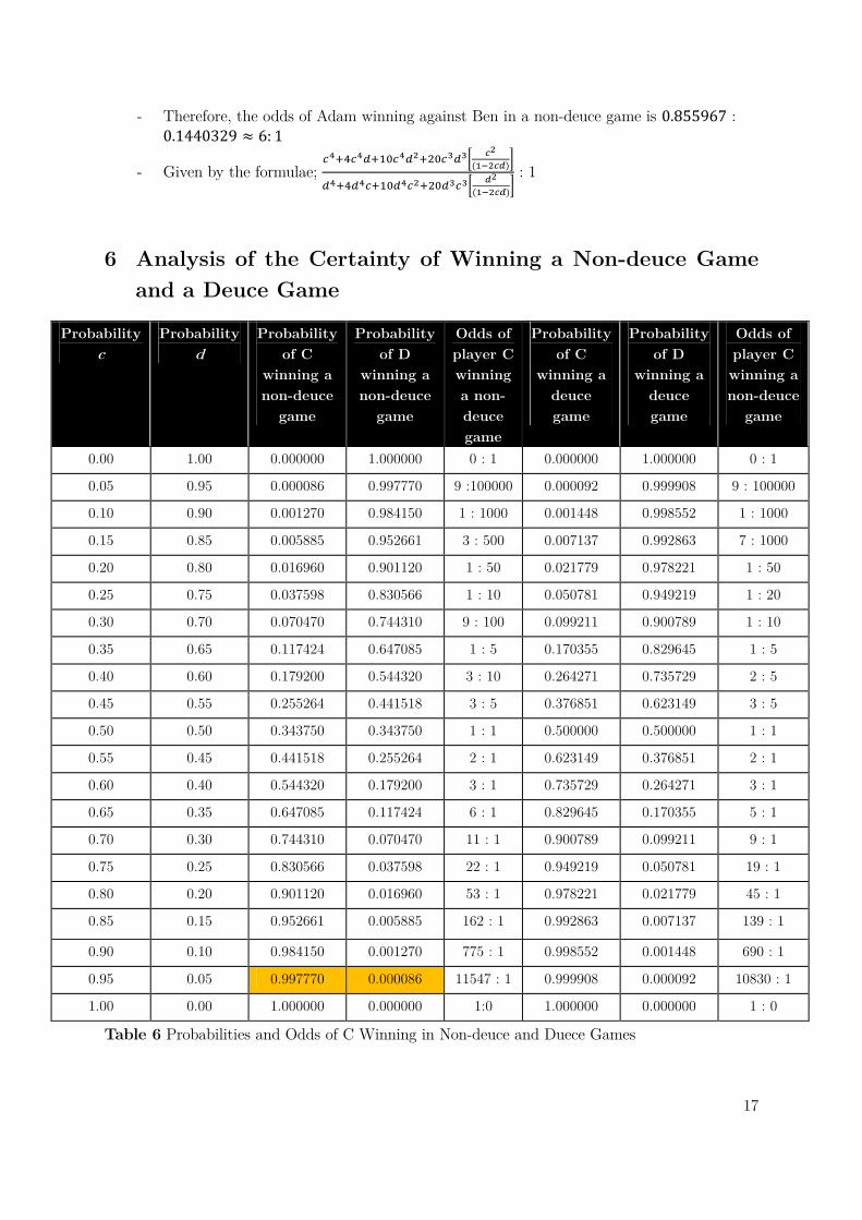
- Therefore, the odds of Adam winning against Ben in a non-deuce game is 0.855967 : 0.1440329 ≈ 6: 1

- Given by the formulae; ��������������������� �

�

(�����)�

��������������������� ��

(�����)� : 1

6 Analysis of the Certainty of Winning a Non-deuce Game

and a Deuce Game

Probability

c

Probability

d

Probability

of C

winning a

non-deuce

game

Probability

of D

winning a

non-deuce

game

Odds of

player C

winning

a non-

deuce

game

Probability

of C

winning a

deuce

game

Probability

of D

winning a

deuce

game

Odds of

player C

winning a

non-deuce

game

0.00 1.00 0.000000 1.000000 0 : 1 0.000000 1.000000 0 : 1

0.05 0.95 0.000086 0.997770 9 :100000 0.000092 0.999908 9 : 100000

0.10 0.90 0.001270 0.984150 1 : 1000 0.001448 0.998552 1 : 1000

0.15 0.85 0.005885 0.952661 3 : 500 0.007137 0.992863 7 : 1000

0.20 0.80 0.016960 0.901120 1 : 50 0.021779 0.978221 1 : 50

0.25 0.75 0.037598 0.830566 1 : 10 0.050781 0.949219 1 : 20

0.30 0.70 0.070470 0.744310 9 : 100 0.099211 0.900789 1 : 10

0.35 0.65 0.117424 0.647085 1 : 5 0.170355 0.829645 1 : 5

0.40 0.60 0.179200 0.544320 3 : 10 0.264271 0.735729 2 : 5

0.45 0.55 0.255264 0.441518 3 : 5 0.376851 0.623149 3 : 5

0.50 0.50 0.343750 0.343750 1 : 1 0.500000 0.500000 1 : 1

0.55 0.45 0.441518 0.255264 2 : 1 0.623149 0.376851 2 : 1

0.60 0.40 0.544320 0.179200 3 : 1 0.735729 0.264271 3 : 1

0.65 0.35 0.647085 0.117424 6 : 1 0.829645 0.170355 5 : 1

0.70 0.30 0.744310 0.070470 11 : 1 0.900789 0.099211 9 : 1

0.75 0.25 0.830566 0.037598 22 : 1 0.949219 0.050781 19 : 1

0.80 0.20 0.901120 0.016960 53 : 1 0.978221 0.021779 45 : 1

0.85 0.15 0.952661 0.005885 162 : 1 0.992863 0.007137 139 : 1

0.90 0.10 0.984150 0.001270 775 : 1 0.998552 0.001448 690 : 1

0.95 0.05 0.997770 0.000086 11547 : 1 0.999908 0.000092 10830 : 1

1.00 0.00 1.000000 0.000000 1:0 1.000000 0.000000 1 : 0

Table 6 Probabilities and Odds of C Winning in Non-deuce and Duece Games

18

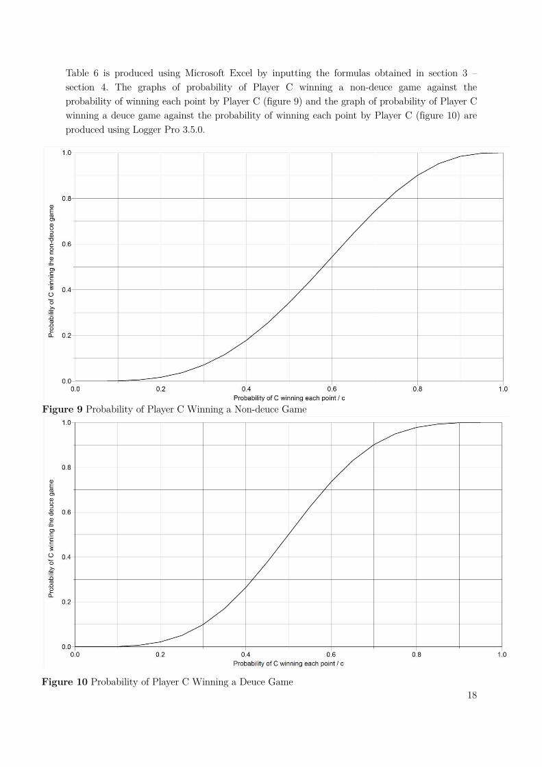
Figure 10 Probability of Player C Winning a Deuce Game

Figure 9 Probability of Player C Winning a Non-deuce Game

Table 6 is produced using Microsoft Excel by inputting the formulas obtained in section 3 –

section 4. The graphs of probability of Player C winning a non-deuce game against the

probability of winning each point by Player C (figure 9) and the graph of probability of Player C

winning a deuce game against the probability of winning each point by Player C (figure 10) are

produced using Logger Pro 3.5.0.

19

2-1

2-2

3-2 2-3

2-4 Lose

3-1

4-1

Win

4-2 Win 3-3 Deuce

From figure 9 and figure 10, it can be seen that when the probability of winning each point is

above 0.8, one player is almost certain to win the game. This seems pretty obvious.

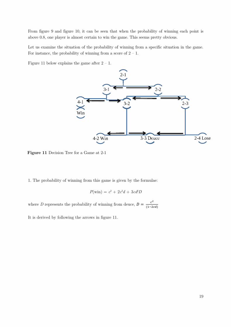
Let us examine the situation of the probability of winning from a specific situation in the game.

For instance, the probability of winning from a score of 2 – 1.

Figure 11 below explains the game after 2 – 1.

1. The probability of winning from this game is given by the formulae:

P(win) = c2 + 2c2d + 3cd2D

where D represents the probability of winning from deuce, � � ��

�������

It is derived by following the arrows in figure 11.

Figure 11 Decision Tree for a Game at 2-1

20

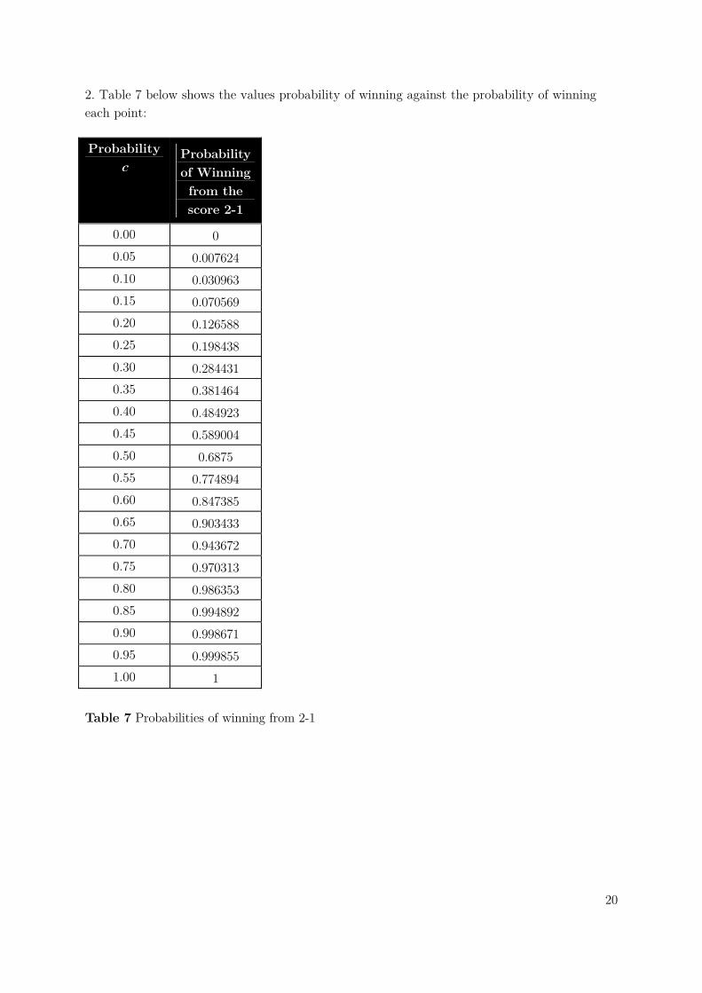
2. Table 7 below shows the values probability of winning against the probability of winning

each point:

Probability

c Probability

of Winning

from the

score 2-1

0.00 0

0.05 0.007624

0.10 0.030963

0.15 0.070569

0.20 0.126588

0.25 0.198438

0.30 0.284431

0.35 0.381464

0.40 0.484923

0.45 0.589004

0.50 0.6875

0.55 0.774894

0.60 0.847385

0.65 0.903433

0.70 0.943672

0.75 0.970313

0.80 0.986353

0.85 0.994892

0.90 0.998671

0.95 0.999855

1.00 1

Table 7 Probabilities of winning from 2-1

21

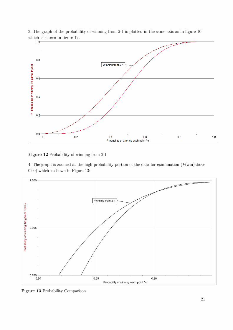
3. The graph of the probability of winning from 2-1 is plotted in the same axis as in figure 10

which is shown in figure 12.

Figure 12 Probability of winning from 2-1

4. The graph is zoomed at the high probability portion of the data for examination (P(win)above

0.90) which is shown in Figure 13:

Figure 13 Probability Comparison

22

From figure 13, we can deduce that the likeliness of winning the game has gone down since the

curve of winning from 2-1 is flatter than the curve in comparison. This is contradicting to our

intuition that even though we are ahead by one point, losing that single point has decreased

the probability of winning the game.

One explanation for that could be, at higher probability of winning each point the chances of

losing a point is very small as seen in table 6 in the shaded cells. As a result, this smaller

chance of losing a point and if the point is lost, may affect the certainty of winning largely.

Also, this explanation supported by another factor that the two curves do not intersect at any

point when the probability of winning each point is less than 0.90 (Figure 12), which suggests

us that when the probability is low, losing a point does not affect the certainty of winning to

that extent.

23

7 Usefulness of Probability Models in Tennis

The probability models for Tennis can prove to be very useful as they show statistics about the

game, the player performance, and most importantly, attempt to answer the question that

everyone looks forward to: “Who will win?”.

It can be used by coaches in training the player and work on what element of technique does the

player need to improve on, as the models describe about the player’s performance. Also, to a

player it might be useful, as it may give a hint to the opponent’s weaknesses by modelling the

opponent’s game play.

It can be used by commentators to support their comments throughout the game and make the

forecast more lively, and interesting. Thus, it may also benefit the TV viewers as they get close

to the certainty of their favourite player winning or losing.

8 Conclusion

The probability models for tennis can lead to the development of other models for other racquet

sports such as badminton, squash, table-tennis etc. since the scoring system is quite similar

among these sports; and thus benefitting from the usefulness of such models. With constraints to

its limitations as described in section 2.2, it can make us closer to the prediction of certainty.

Also, there is no harm in being fascinated by the pattern of these probabilistic numbers as they

tell us more truth than we can actually perceive through naked eye.