Embed Size (px)
Citation preview
MODELLING, SIMULATION AND ANALYSIS OF LOW-COST DIRECT
TORQUE CONTROL OF PMSM USING HALL-EFFECT SENSORS
A Thesis
by
SALIH BARIS OZTURK
Submitted to the Office of Graduate Studies of Texas A&M University
in partial fulfillment of the requirements for the degree of
MASTER OF SCIENCE
December 2005
Major Subject: Electrical Engineering

MODELLING, SIMULATION AND ANALYSIS OF LOW-COST DIRECT
TORQUE CONTROL OF PMSM USING HALL-EFFECT SENSORS
A Thesis
by
SALIH BARIS OZTURK
Submitted to the Office of Graduate Studies of Texas A&M University
in partial fulfillment of the requirements for the degree of
MASTER OF SCIENCE
Approved by: Chair of Committee, Hamid A. Toliyat Committee Members, Prasat N. Enjeti S. P. Bhattacharyya Reza Langari Head of Department, Costas N. Georghiades
December 2005
Major Subject: Electrical Engineering

iii
ABSTRACT
Modelling, Simulation and Analysis of Low-Cost Direct Torque Control
of PMSM Using Hall-Effect Sensors. (December 2005)
Salih Baris Ozturk, B.S., Istanbul Technical University
Chair of Advisory Committee: Dr. Hamid A. Toliyat
This thesis focuses on the development of a novel Direct Torque Control (DTC)
scheme for permanent magnet (PM) synchronous motors (surface and interior types) in
the constant torque region with the help of cost-effective hall-effect sensors. This
method requires no DC-link sensing, which is a mandatory matter in the conventional
DTC drives, therefore it reduces the cost of a conventional DTC of a permanent magnet
(PM) synchronous motor and also removes common problems including; resistance
change effect, low speed and integration drift. Conventional DTC drives require at least
one DC-link voltage sensor (or two on the motor terminals) and two current sensors
because of the necessary estimation of position, speed, torque, and stator flux in the
stationary reference frame.
Unlike the conventional DTC drive, the proposed method uses the rotor reference
frame because the rotor position is provided by the three hall-effect sensors and does not
require expensive voltage sensors. Moreover, the proposed algorithm takes the
acceleration and deceleration of the motor and torque disturbances into account to
improve the speed and torque responses.
The basic theory of operation for the proposed topology is presented. A
mathematical model for the proposed DTC of the PMSM topology is developed. A
simulation program written in MATLAB/SIMULINK® is used to verify the basic
operation (performance) of the proposed topology. The mathematical model is capable
of simulating the steady-state, as well as dynamic response even under heavy load
conditions (e.g. transient load torque at ramp up). It is believed that the proposed system

iv
offers a reliable and low-cost solution for the emerging market of DTC for PMSM
drives.
Finally the proposed drive, considering the constant torque region operation, is
applied to the agitation part of a laundry washing machine (operating in constant torque
region) for speed performance comparison with the current low-cost agitation cycle
speed control technique used by washing machine companies around the world.

v
To my mother and father.

vi
ACKNOWLEDGMENTS
There is a numerous amount of people I need to thank for their advice, help,
assistance and encouragement throughout the completion of this thesis.
First of all, I would like to thank my advisor, Dr. Hamid A. Toliyat, for his
support, continuous help, patience, understanding and willingness throughout the period
of the research to which this thesis relates. Moreover, spending his precious time with
me is appreciated far more than I have words to express. I am very grateful to work with
such a knowledgeable and insightful professor. To me he is more than a professor; he is
like a father caring for his students during their education. Before pursuing graduate
education in the USA I spent a great amount of time finding a good school, and more
importantly a quality professor to work with. Even before working with Dr. Toliyat I
realized that the person who you work with is more important than the prestige at the
university in which you attend.
I would also like to thank the members of my graduate study committee,
Dr. Prasad Enjeti, Dr. S.P. Bhattacharyya, and Dr. Reza Langari for accepting my
request to be a part of the committee.
I would like to extend my gratitude to my fellow colleagues in the Advanved
Electric Machine and Power Electronics Laboratory: our lab manager Dr. Peyman Niazi,
Dr. Leila Parsa, Dr. M.S. Madani, Dr. Namhun Kim, Dr. Mesuod Haji, Dr. Sang-Shin
Kwak, Dr. Mehdi Abolhassani, Bilal Akin, Steven Campbell, Salman Talebi, Rahul
Khopkar, and Sheab Ahmed. I cherish their friendship and the good memories I have
had with them since my arrival at Texas A&M University.
Also, I would like to thank to the people who are not participants of our lab but
who are my close friends and mentors who helped, guided, assisted and advised me
during the completion of this thesis: Onur Ekinci, David Tarbell, Ms. Mina Rahimian,
Dr. Farhad Ashrafzadeh, Peyman Asadi, Sanjey Tomati, Neeraj Shidore, Steve Welch,
Burak Kelleci, Guven Yapici, Murat Yapici, Cansin Evrenosoglu, Ali Buendia, Kalyan
Vadakkeveedu, Leonardo Palma and many others whom I could not mention here.

vii
I would also like to acknowledge the Electrical Engineering department staff at
Texas A&M University: Ms. Tammy Carda, Ms. Linda Currin, Ms. Gayle Travis and
many others for providing an enjoyable and educational atmosphere.
Last but not least, I would like to thank my parents for their patience and endless
financial, and more importantly, moral support throughout my life. First, I am very
grateful to my dad for giving me the opportunity to study abroad to earn a good
education. Secondly, I am very grateful to my mother for her patience which gave me a
glimpse of how strong she is. Even though they do not show their emotion when I talk to
them, I can sense how much they miss me when I am away from them. No matter how
far away from home I am, they are always there to support and assist me. Finally, to my
parents, no words can express my gratitude for you and all the things you sacrifice for
me.

viii
TABLE OF CONTENTS
Page
ABSTRACT ......................................................................................................................iii
ACKNOWLEDGMENTS.................................................................................................vi
TABLE OF CONTENTS ................................................................................................viii
LIST OF FIGURES...........................................................................................................xi
LIST OF TABLES .........................................................................................................xxii
CHAPTER
I INTRODUCTION..................................................................................................1
1.1 Principles of DC Brush Motors and Their Problems .................................1 1.2 Mathematical Model of the DC Brush Motor ............................................6 1.3 AC Motors and Their Trend.....................................................................10 1.4 Thesis Outline ..........................................................................................12
II BASIC OPERATIONAL PRINCIPLES OF PERMANENT MAGNET SYNCHRONOUS AND BRUSHLESS DC MOTORS ......................................14
2.1 Permanent Magnet Synchronous Motors (PMSMs) ................................14 2.1.1 Mathematical Model of PMSM.................................................20
2.2 Introduction to Brushless DC (BLDC) Motors ........................................36 2.2.1 Mathematical Model of BLDC Motor ......................................39
2.3 Mechanical Structure of Permanent Magnet AC Motors (PMSM and BLDC .......................................................................................................45
2.4 Advantages and Disadvantages of PMSM and BLDC Motors ................49 2.5 Torque Production Comparison of PMSM and BLDC Motors ...............53 2.6 Control Principles of the BLDC Motor....................................................55 2.7 Control Principles of the PM Synchronous Motor...................................62
III MEASUREMENTS OF THE PM SPINDLE MOTOR PARAMETERS ...........67
3.1 Introduction ..............................................................................................67 3.2 Principles of Self-Commisioning with Identification ..............................68 3.3 Resistance and dq-axis Synchronous Inductance Measurements.............69 3.4 Measurment of the Back-EMF Constant and Rotor Flux Linkage ..........79 3.5 Load Angle Measurement ........................................................................81

ix
CHAPTER Page
IV OPEN-LOOP SIMULINK® MODEL OF THE PM SPINDLE MOTOR ...........88
4.1 Principles of PMSM Open-Loop Control ................................................88 4.2 Building Open-Loop Steady and Transient-State Models .......................90 4.3 Power Factor and Efficiency Calculations in Open-Loop
Matlab/Simulink® Model .........................................................................97
V CONVENTIONAL DIRECT TORQUE CONTROL (DTC) OPERATION OF PMSM DRIVE ...............................................................................................99
5.1 Introduction and Literature Review .........................................................99 5.2 Principles of Conventional DTC of PMSM Drive .................................107
5.2.1 Torque Control Strategy in DTC of PMSM Drive..................108 5.2.2 Flux Control Strategy in DTC of PMSM Drive......................112 5.2.3 Voltage Vector Selection in DTC of PMSM Drive ................107
5.3 Control Strategy of DTC of PMSM Drive .............................................120
VI PROPOSED DIRECT TORQUE CONTROL (DTC) OPERATION OF PMSM DRIVE ...................................................................................................124
6.1 Introduction and Principles of the Proposed DTC Drive .......................124 6.2 Position and Speed Estimation Method with Low Resolution Position
Sensor .....................................................................................................130
VII AGITATION CYCLE SPEED CONTROL OF VERTICAL-AXIS LAUNDRY MACHINE.....................................................................................135
7.1 Modern Washing Machines: Top Loaded (Vertical-axis) and Front Loaded (Horizontal-axis) Washine Machines........................................135
7.2 Introduction to Speed Control of a BLDC Spindle Motor (48 Pole/ 36 Slot) in the Agitation Cycle of a Washing Machine .........................136
7.3 Agitate Washer Controller Model in SIMPLORER® ............................138
VIII EXPERIMENTAL AND SIMULATION ANALYSIS.....................................148
8.1 Open-Loop Simulation vs. Experimental Results ..................................148 8.1.1 Open-Loop Steady-State and Transient Analysis (Simulation).............................................................................148 8.1.2 Open-Loop Steady-State and Transient Analysis (Experiment)............................................................................152 8.1.3 System Configuration for Electrical Parameters
Measurements..........................................................................154 8.1.4 The M-Test 4.0 Software ........................................................156 8.1.5 Curve Testing ..........................................................................157
8.2 Experimental vs. Simulation Results (Commercial Agitation Control).158 8.2.1 Complete Agitation Speed Control Analysis (Steady-State) ..159

x
CHAPTER Page
8.2.2 Complete Agitation Speed Control Analysis (Transient and Steady-States)..........................................................................169
8.2.3 Simulation Results of the Proposed DTC Method Used in Agitation Cycle Speed Control ...............................................176 8.2.3.1 Transient and Steady-State Response Under Load
Condition..................................................................181 8.2.3.2 Effects of Stator Resistance Variation in
Conventional DTC with Encoder .............................195 8.2.3.3 Drift Problem Occurs in Conventional DTC Scheme .....................................................................209 8.2.3.4 Overview of the Offset Error Occured in the
Proposed DTC Scheme ............................................213 8.2.3.5 Overview of the Rotor Flux Linkage Error Occured
in the Proposed DTC Scheme ..................................218
IX SUMMARY AND FUTURE WORK................................................................224
9.1 Summary of the Work and Conclusion ..................................................224 9.2 Future Work ...........................................................................................225
REFERENCES...............................................................................................................227
APPENDIX A ................................................................................................................232
VITA ..............................................................................................................................237

xi
LIST OF FIGURES
FIGURE Page
1.1. Basic model of a DC brush motor ....................................................................2 1.2. Fundamental operation of a DC brush motor (Step 1). ....................................4 1.3. Fundamental operation of a DC brush motor (Step 2). ....................................5 1.4. Fundamental operation of a DC brush motor (Step 3). ....................................6 1.5. Electrical circuit model of a separately excited
DC brush motor (transient-state)......................................................................7 1.6. Electrical circuit model of a separately excited
DC brush motor (steady-state) .........................................................................8
2.1. Two-pole three phase surface mounted PMSM. ............................................22 2.2. Q-axis leading d-axis and the rotor angle represented as ..........................26 rθ 2.3. Q-axis leading d-axis and the rotor angle represented as θ ...........................28 2.4. Line-to-line back-EMF ( ), phase back-EMFs, phase current abE
waveforms and hall-effect position sensor signals for a BLDC motor ..........38
2.5. Equivalent circuit of the BLDC drive (R, L and back-EMF).........................40 2.6. Simplified equivalent circuit of the BLDC drive
(R, (L-M) and back-EMF)..............................................................................42
2.7. Cross sectional view of four pole surface-mounted PM rotor ( d qL L= ) .......46 2.8. Cross sectional view of four pole interior-mounted PM rotor ( d qL L≠ ).......47 2.9. Ideal BLDC operation ....................................................................................55 2.10. PMSM controlled as BLDC ...........................................................................55 2.11. Voltage Source Inverter (VSI) PMAC drive..................................................55

xii
FIGURE Page
2.12. Voltage Source Inverter (VSI) BLDC drive ..................................................56 2.13. A typical current-controlled BLDC motor drive with position
feedback .........................................................................................................59
2.14. Six possible switching sequences for a three-phase BLDC motor.................60 2.15. PWM current regulation for BLDC motor [8] ...............................................61 2.16. Basic phasor diagram for PMSM [8] .............................................................63 2.17. Basic block diagram for high-performance torque control
for PMSM [8] .................................................................................................64 2.18. Basic block diagram for high-performance torque control
for PMSM [8] .................................................................................................65 2.19. Basic block diagram for high-performance torque control
for PMSM [8] .................................................................................................65 3.1. Vector phasor diagram for non-salient PMSM ..............................................72 3.2. Measurement of phase resistance and inductance..........................................74 3.3. Phase A voltage waveform and hall-effect signal of the same phase ............82 3.4. Rotor magnet representation along with hall-effect signals...........................83 3.5. Phase A voltage waveform and hall-effect signal with jittering effect ..........83 3.6. Experimental vs. simulated load angle (deg.) at 20 Hz (No-load) .................85 3.7. Experimental vs. simulated load angle (deg.) at 40 Hz (No-load) .................86 3.8. Experimental vs. simulated load angle (deg.) at 40 Hz (Load)......................86 3.9. Possible vector representation of PMSM .......................................................87 4.1. Basic open-loop block diagram of PMSM.....................................................89 4.2. Overall open-loop control block diagram of PMSM in SIMULINK®...........91

xiii
FIGURE Page
4.3. Abc to stationary and stationary to dq rotor reference
frame transformation block ............................................................................91
4.4. Rotor reference frame and stationary reference frame coordinate representation ...............................................................................92
4.5. Dq rotor reference frame to stationary and stationary to
abc transformation block................................................................................93
4.6. Steady state dq-axis rotor reference frame motor model ...............................94 4.7. Rotor ref. frame, synchronous ref. frame, and stationary ref. frame
representation as vectors ................................................................................96
5.1. Eight possible voltage space vectors obtained from VSI.............................100 5.2. Circular trajectory of stator flux linkage in the stationary DQ-plane ..........101 5.3. Phasor diagram of a non-saliet pole synchronous machine in
the motoring mode .......................................................................................108
5.4. Electrical circuit diagram of a non-salient synchronous machine at constant frequency (speed) ........................................................109
5.5. Rotor and stator flux linkage space vectors
(rotor flux is lagging stator flux) ..................................................................112
5.6. Incremental stator flux linkage space vector representation in the DQ-plane ......................................................................................................112
5.7. Representation of direct and indirect components of
the stator flux linkage vector ........................................................................114
5.8. Voltage Source Inverter (VSI) connected to the R-L load...........................116 5.9. Voltage vector selection when the stator flux vector is located in sector i ..117
5.10. Basic block diagram of DTC of PMSM.......................................................120
6.1. Hall-effect sensor placement shown in DQ stationary reference frame.......125

xiv
FIGURE Page
6.2. Representation of the rotor and stator flux linkages both in the synchronous dq and stationary DQ-planes...................................................127
6.3. Block diagram of the proposed DTC of PMSM ..........................................129
6.4. Speed and position estimation using low-resolution position sensor...........131 6.5. Representation of acceleration and speed at the sectors
and at the hall-effect sensors, respectively...................................................134
7.1. Simple flowchart of the commercial agitation speed control [57] ...............138 7.2. Reference speed profile for the agitation speed control
in a washing machine ...................................................................................139 7.3. Detailed flowchart of the simple agitation speed control
of a washing machine [58] ...........................................................................140
7.4. PWM increment during the ramp time [58] .................................................143 7.5. Speed response during ramp up when PWM is incremented
at every PT time [58] ...................................................................................144
7.6. Ideal speed profile of the agitation speed control [58].................................146 7.7. Typical practical speed response of the agitation speed control [58]...........147 8.1. Efficiency, power factor, motor current (Phase A), and
motor speed versus applied load torque (open-loop exp. and sim.) at 100 rpm with V / f ~= 2 ..........................................................................150
8.2. Dynamic speed response of exp. and sim. when V / f = 18/15 (0-37.5 rpm) .................................................................................................151
8.3. Dynamic speed response of exp. and sim. when V / f = 1 (0-37.5 rpm) .................................................................................................151
8.4. Torque response of PMSM when it is supplied by quasi-square wave
currents .........................................................................................................152

xv
FIGURE Page
8.5. Efficiency, power factor, motor current (Phase A), and motor speed versus applied load torque (experimental, open-loop)
at 100 rpm with V / f ~= 2 ..........................................................................154
8.6. Basic block diagram of overall system for efficiency measurements ..........155 8.7. Overall system configuration .......................................................................156 8.8. Sample curve test .........................................................................................158 8.9. Graphical representation of the sample curve test .......................................158 8.10. Input current of the single phase diode rectifier at 10 N·m of load torque..159 8.11. Input current to the single phase diode rectifier (experiment)
at 10 N·m of load torque (100 rpm).............................................................160 8.12. Voltage source obtained from the wall plug ................................................161 8.13. DC-link voltage of the VSI at 10 N·m of load torque (100 rpm) .................162 8.14. Steady-state load torque and plateau speeds (experiment and
simulation) at 10 N·m of load torque (100 rpm) ..........................................163 8.15. Steady-state electromagnetic torque (simulation) at 10 N·m of load
torque (100 rpm)...........................................................................................164
8.16. Block diagram of the overall commercialized agitation washer control with the trapezoidal voltage waveform and efficiency calculation and measurement.................................................................................................165
8.17. Experimental three-phase motor phase currents at 10 N·m of
load torque (100 rpm)...................................................................................166
8.18. Simulated three-phase motor phase currents at 10 N·m of load torque (100 rpm)...................................................................................167
8.19. Exp. PF., eff., and sim. PF., eff. vs. torque at 10 N·m (100 rpm).................167
8.20. Block diagram of the overall commercialized agitation washer control
with trapezoidal voltage waveform ..............................................................168

xvi
FIGURE Page
8.21. Experimental and simulation speed response (transient and steady-state) at no-load......................................................................................................170
8.22. Experimental and simulation speed response (transient and steady-state)
at 5 N·m of load torque.................................................................................171
8.23. Experimental and simulation speed response (transient and steady-state) at no-load (0.7 second ramp time)................................................................172
8.24. Rotor position obtained in simulation ..........................................................173 8.25. Steady-state SIMPLORER® model of the agitation speed control ..............174 8.26. SIMPLORER® model of commercialized overall agitation speed
control system (transient+steady-state) ........................................................175
8.27. Agitation speed control test-bed...................................................................176 8.28. Load torque ( LT ), , , and at a 0.35 second ramp time emrefT emestT emactT
when the PI integrator initial value is 7 N·m................................................182 8.29. sλ
∗ (Reference Stator Flux), _s estλ and _s actλ at a 0.35 second ramp time when the PI integrator initial value is 7 N·m................................................183
8.30. sDλ and sQλ circular trajectory at a 0.35 second ramp time when
the PI integrator initial value is 7 N·m .........................................................183 8.31. Load torque ( LT ), , , and at a 0.35 second ramp time emrefT emestT emactT
when the PI integrator initial value is 8.5 N·m.............................................184
8.32. sλ∗ (Reference Stator Flux), _s estλ and _s actλ at a 0.35 second ramp time
when the PI integrator initial value is 8.5 N·m.............................................185
8.33. sDλ and sQλ circular trajectory at a 0.35 second ramp time when the PI integrator initial value is 8.5 N·m ......................................................186
8.34. Phase-A current ( ), , and when a 0.35 second ramp time asi dqracti dqresti
is used when the PI integrator initial value is 7 N·m....................................187
xvii
FIGURE Page
8.35. Phase-A current ( ), , and when a 0.35 second ramp time asi dqracti dqresti is used when the PI integrator initial value is 8.5 N·m.................................188
8.36. Reference and actual speed, speed error (ref-act), actual and estimated
position when a 0.35 second ramp time is used when the PI integrator initial value is 7 N·m ....................................................................................189
8.37. Reference and actual speed, speed error (ref-act), and actual and
estimated position when a 0.35 second ramp time is used when the PI integrator initial value is 8.5 N·m.................................................................190
8.38. , , and at a 0.6125 second ramp time when emrefT emestT emactT
the PI integrator initial value is 7 N·m .........................................................191 8.39. sλ
∗ (reference stator flux), _s estλ and _s actλ at 0.6125 second ramp time when PI integrator initial value is 7 N·m......................................................192
8.40. sDλ (X axis) and sQλ (Y axis) circular trajectory at a 0.6125 second ramp
time when the PI integrator initial value is 7 N·m........................................193 8.41. Phase-A current ( ), , and when a 0.6125 second ramp time asi dqracti dqresti
is used when the PI integrator initial value is 7 N·m....................................194
8.42. Reference and actual speeds, speed error (ref-act), and actual and estimated positions when a 0.6125 second ramp time is used when the PI integrator initial value is 7 N·m....................................................................195
8.43. Reference and actual speeds, actual position, and three phase currents
when a 0.35 second ramp time is used (no initial torque, just ramp rate is added). Stator resistance change effect is not applied................................196
8.44. , , and at a 0.35 second ramp time. Stator resistance emrefT emestT estFlux
change effect is not applied..........................................................................197

xviii
FIGURE Page
8.45. Load torque (TL), , , , and estimated stator flux linkage emrefT emestT emactT under step stator resistance change (1.5x sR ) at 0 second when ramp time is 0.35 second when the initial integrator value of the PI is chosen
as 7 N·m........................................................................................................198
8.46. Reference and actual speeds, actual position, and three phase currents when a 0.35 second ramp time is used (no initial torque, just ramp rate is added). Stator resistance is increased by 1.5x sR at 0 second ......................199
8.47. Reference and actual speeds, speed error (ref-act), actual position, and
three phase currents when a 0.35 second ramp time is used (no initial torque, just ramp rate is added). Stator resistance is increased by 1.5x sR at 0.675 second ............................................................................................200
8.48. , , and at a 0.35 second ramp time. Stator resistance emrefT emestT estFlux
is increased by 1.5x sR at 0.675 second .......................................................201
8.49. , , , , estimated and real rotor positions with a emestT emactT estFlux actFlux 0.35 second ramp time. Stator resistance is increased by 1.5x sR at 0.675
second...........................................................................................................202 8.50. , , , , estimated and real rotor positions with a emestT emactT estFlux actFlux
0.35 second ramp time. Stator resistance is increased by 1.5x sR at 0.35/2 second ( V).....................................................................................203 370dcV =
8.51. Reference and actual speeds, and three phase currents when a 0.35 second
ramp time is used (no initial torque, just ramp rate is added). Stator resistance is increased by 1.5x sR at 0.35/2 second ( 370dcV = V) ...............204
8.52. , , and with a 0.35 second ramp time. Stator resistance emestT emactT estFlux
is increased by 1.5x sR at 0.35/2 second ( 370dcV = V) ................................205
8.53. Estimated sDλ (X axis) and sQλ (Y axis) circular trajectory with a 0.35 second ramp time. Stator resistance is increased by 1.5x sR at 0.675 second (kp=9, ki=3)......................................................................................206

xix
FIGURE Page
8.54. Estimated sDλ (X axis) and sQλ (Y axis) circular trajectory with a 0.35 second ramp time. Stator resistance is increased by 1.5x sR at 0.35/2 second (kp=9, ki=3)......................................................................................207
8.55. Actual sDλ (X axis) and sQλ (Y axis) circular trajectory with a 0.35
second ramp time. Stator resistance is increased by 1.5x sR at 0.35/2 second (stopped at 0.28 s.) ...........................................................................208
8.56. Actual sDλ (X axis) and sQλ (Y axis) circular trajectory with a 0.35
second ramp time. Stator resistance is increased by 1.5x sR at 0.675 second (stopped at 0.28 s.) ...........................................................................209
8.57. Reference and actual speeds, actual position, and three phase
currents when a 0.35 second ramp time is used (no initial torque, just ramp rate is added. A 0.1 A current offset is added to the D- and Q-axes currents in the SRF ( 370dcV = V).................................................................211
8.58. Load torque (TL), , , , and actual stator flux linkage. emrefT emactT estFlux
A 0.1 A offset occurs on the D- and Q-axes currents in the SRF when the ramp time is 0.35 second..............................................................................212
8.59. Estimated sDλ (X axis) and sQλ (Y axis) circular trajectory with a 0.35
second ramp time. A 0.1 A offset is included in the D- and Q-axes currents in the SRF ( 370dcV = V). (kp=9, ki=3) ..........................................213
8.60. Reference and actual speeds, speed error (ref-act), estimated and
actual positions when a 0.35 second ramp time is used (7.5 N·m. initial torque is used in the PI’s integrator with appropriate ramp rate). A 0.1 A offset is included in the d- and q-axes currents in the RRF ( V) ...214 370dcV =
8.61. Phase-A current ( ), , and when a 0.35 second ramp time is asi dqracti dqresti
used with a PI integrator initial value of 7.5 N·m. A 0.1 A offset is include to the d- and q-axes currents in the RRF ( 370dcV = V)...................215

xx
FIGURE Page
8.62. Load torque (TL), , , and . A 0.1 A offset occurs on d- and q-axes currents in the RRF when ramp time is 0.35 second ( 3 V)................................................................................................216
emrefT emestT emactT
70dcV =
8.63. , , when a 0.35 second ramp time is used with a PI integrator initial value of 7.5 N·m. A 0.1 A offset is included in the d- and q-axes currents in the RRF (
refFlux estFlux actualFlux
370dcV = V)..........................................217 8.64. Estimated sDλ (X axis) and sQλ (Y axis) circular trajectory at a 0.35
second ramp time with a PI integrator initial value of 7.5 N·m. A 0.1 A offset is included in the d- and q-axes currents in the RRF ( V). (kp=9, ki=3)..................................................................................................218
370dcV =
8.65. Reference and actual speeds, speed error (ref-act), estimated and
actual positions when a 0.35 second ramp time is used (7 N·m. initial torque is used in the PI’s integrator with appropriate ramp rate). 0.7x is used at 0.35/2 sec. in the motor model (
rλ370dcV = V). (kp=9, ki=3) ..........219
8.66. Phase-A current ( ), , and when a 0.35 second ramp time is
used with a PI integrator initial value of 7 N·m. 0.7x is used at 0.35/2 second in the motor model (
asi dqracti dqresti
rλ370dcV = V). (kp=9, ki=3)...............................220
8.67. Load torque (TL), , , and . 0.7x is used at emrefT emestT emactT rλ
0.35/2 second in the motor model ( 370dcV = V). (kp=9, ki=3)....................221
8.68. refFlux , , when a 0.35 second ramp time is used with a PI integrator initial value of 7 N·m. 0.7x is used at 0.35/2 second in the motor model ( V). (kp=9, ki=3).....................................................222
estFlux actualFlux
rλ370dcV =
8.69. Estimated sDλ (X axis) and sQλ (Y axis) circular trajectory at a 0.35
second ramp time with a PI integrator initial value of 7 N·m. 0.7x is used 0.35/2 second in the motor model (
rλ370dcV = V). (kp=9, ki=3) ...........223

xxi
FIGURE Page
A-1. Specifications of the Fujitsu MB907462A microcontroller.. .......................234
A-2. Theoretical background of active power, apparent power, power factor and connection of the power analyzer to the load (motor)...........................236
A-3. MATLAB/SIMULINK® model of the proposed DTC ................................237

xxii
LIST OF TABLES
TABLE Page
3.1 Measurements of Self-Resistance and Self-Inductance .................................76
3.2 Measurements of Line-to-Neutral Back-EMF for Each Phase (0-50 rpm) ...................................................................................81
5.1 Switching Table............................................................................................118

1
CHAPTER I
INTRODUCTION
1.1. Principles of DC Brush Motors and Their Problems
DC motors have been the most widespread choice for use in high performance
systems. The main reason for their popularity is the ability to control their torque and
flux easily and independently. In DC brush machines, the field excitation that provides
the magnetizing current is occasionally provided by an external source, in which case the
machine is said to be separately excited. In particular, the separately excited DC motor
has been used mainly for applications where there was a requirement for fast response
and four-quadrant operation with high performance near zero speed.
Generally in DC brush motors, flux is controlled by manipulating field winding
current and torque by changing the armature winding current. The trade-off is less
rugged motor construction, which requires frequent maintenance and an eventual
replacement of the brushes and commutators. It also precludes the use of a DC motor in
hazardous environments where sparking is not permitted. Moreover, there is a potential
drop called ‘contact potential difference’, associated with this arrangement, and is
usually in the range of 1-1.5 V, leading to a drop in the effective input voltage.
The well-known DC brush motor, like any other rotating machine, has a stator
and rotor (as shown in Fig. 1.1). On the stator (stationary part), there is a magnetic field
which can be provided either by permanent magnets or by excited field windings on the
stator poles. On the rotor, the main components are the armature winding, armature core,
a mechanical switch called commutator which rotates, and a rotor shaft. The commutator
___________________ This thesis follows the style and format of IEEE Transactions on Industry Applications.

2
segments are insulated from one another and from the clamp holding them. In addition to
that brushes, the stationary external components of the rotor, together with the
commutator act not only as rotary contacts between the coils of the rotating armature and
the stationary external circuit, but also as a switch to commutate the current to the
external DC circuit so that it remains unidirectional even though the individual coil
voltages are alternating.
u
vw
+
-
dcV
N
S
Fig. 1.1. Basic model of a DC brush motor.
The maximum torque is produced when the magnetic field of the stator and the
rotor are perpendicular to each other (can be seen in Figs. 1.2 through 1.4,
hypothetically). The commutator makes it possible for the rotor and stator magnetic
fields to always be perpendicular. The commutation thus plays a very important part in
the operation of the DC brush motor. It causes the current through the loop to reverse at
the instant when unlike poles are facing each other. This causes a reversal in the polarity
of the field, changing attractive magnetic force into a repulsive one causing the loop to
continue to rotate.

3
When applying a voltage at the brushes, current flows through two of the coils.
This current interacts with the magnetic field of the permanent magnet and produces
torque. This torque causes to move. When the motor moves the brushes will switch to a
different coil automatically causing the rotor to turn further. If the voltage (armature) is
increased it will turn faster and if the magnetic field of permanent magnet is higher then
it will produce more torque.
Since the back-EMF generated in the coil is short-circuited by the brush, a large
current flows causing sparking at the interface of the commutator and the brushes, as
well as causing heating and the production of braking torque. In order to minimize this
problem, commutation is carried out in the magnetic field crossover region. Even after
taking these measures, because of the distortion of the effective magnetic flux due to the
armature reaction, some back-EMF is still generated in the coils in the magnetic filed
crossover region. It is desirable to minimize the crossover region in order to maximize
the utilization of the motor [1].
In general DC motors, the applied voltage (EMF) is never going to be greater
than back-EMF. The difference between the applied EMF (voltage) and back-EMF is
always such that current can flow in the conductor and produce motion.
Fundamental operation of the DC motor is explained from Figs. 1.2 through 1.4
as follows:
The direction of current flow from the DC voltage source in the figures is based
on electron theory in which current flows from the negative terminal of a source of
electricity to the positive terminal. On the contrary, the older convention supposes that
current flows from positive terminal of a source of electricity through to the negative
terminal [2].
The coil’s pole pair positioning, shown in the figures, is decided by using
Fleming’s left hand rule for generators. If a coil resides in a magnetic field and the
current and rotation of the coil are known, then direction of the magnetic field for the
coil can be found easily by using Fleming’s left hand rule. This rule states that if the
thumb and the first and middle fingers of the left hand are perpendicular to one another,

4
with the first and middle fingers pointing in the flux direction and the thumb pointing in
the direction of motion of the conductor, the middle finger will point in the direction in
which the current flows [2].
With the loop in Fig. 1.2, the current flowing through the coil makes the top of
the loop a north pole and the underside a south pole. This is found by applying the left-
hand rule under the assumption of the back-EMF (direction) is opposite of the direction
of current flow which is provided by DC voltage source [2].
N
S
NS
Fig. 1.2. Fundamental operation of a DC brush motor (Step 1).
The magnetic poles of the loop will be repelled by the like poles and attracted by
the corresponding opposite poles of the field. The coil will therefore rotate clockwise,
attempting to bring the unlike poles together.
When the loop has rotated through 90 degrees, shown in Fig. 1.3, commutation
takes place, and the current through the loop reverses its direction. As a result, the
magnetic field generated by the loop is reversed. Now, like poles face each other which
means that they repel each other and the loop continues to rotate in an attempt to bring
unlike poles together [2].

5
S
N
NS
Fig. 1.3. Fundamental operation of a DC brush motor (Step 2).
Fig. 1.4 shows the loop position after being rotated 180 degrees from Fig. 1.3.
Now the situation is the same as when the loop was back in the position shown in
Fig. 1.3. Commutation takes place once again, and the loop continues to rotate. In this
very basic DC brush motor example, two commutator segments used with one coil loop
for simplicity. Having a small number of commutator segments in DC brush motor
causes torque ripples. As the number of segments increases, the torque fluctuation
produced by commutation is greatly reduced. In a practical machine, for example, one
might have as many as 60 segments, and the variation of the load angle between stator
magnetic flux and rotor flux would only vary ± degrees, with a fluctuation of less than
1 percent. Thus, the DC brush motor can produce a nearly constant torque [3].
3

6
N
S
NS
Fig. 1.4. Fundamental operation of a DC brush motor (Step 3).
1.2. Mathematical Model of the DC Brush Motor
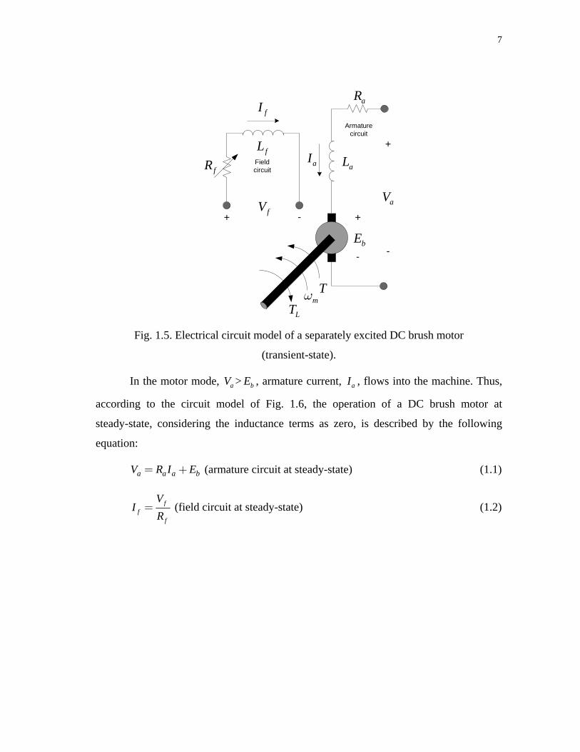
Fig. 1.5 depicts the electrical circuit model of a separately excited DC motor. The
field excitation is shown as a voltage, fV , which generates a field current, fI , that flows
through a variable resistor (which permits adjustment of the field excitation,) fR , and
through the field coil, fL . The armature circuit, on the other hand, consists of a
back-emf, , an armature resistance, bE aR , and an armature voltage, V . a
7
fI
fL
fR
fV
aL
aR
bE
aV+ +
+
-
- -
aI
T
LTmω
Fieldcircuit
Armaturecircuit
Fig. 1.5. Electrical circuit model of a separately excited DC brush motor
(transient-state).
In the motor mode, > , armature current, aV bE aI , flows into the machine. Thus,
according to the circuit model of Fig. 1.6, the operation of a DC brush motor at
steady-state, considering the inductance terms as zero, is described by the following
equation:
a a aV R I E= + b (armature circuit at steady-state) (1.1)
ff
f
VI
R= (field circuit at steady-state) (1.2)

8
fI
fR
fV
aR
bE
aV+ +
+
-
--
aI
T
LTmω
Fieldcircuit
Armaturecircuit
Mechanical Load
Fig. 1.6. Electrical circuit model of a separately excited DC brush motor (steady-state).
The equations describing the dynamic behavior of a separately excited DC brush
motor, as its circuit model in Fig. 1.5 depicts, are as follows:
( )( ) ( ) ( )aa a a a b
dI tV t R I t L E tdt
= + + (Armature circuit at transient-state) (1.3)
( )( ) ( ) f
f f f f
dI tV t R I t L
dt= + (Field circuit at transient-state) (1.4)
The torque developed by the motor can be written as follows:
( )( ) ( ) mem L m
d tT t T B t Jdtω
ω= + + (1.5)
In that equation, the total moment of inertia is represented by such that the
motor is assumed to be rigidly connected to an inertial load. Friction losses in the load
are represented by a viscous friction coefficient by
J
B , and load torque is represented by
, which is typically either constant or some function of speed, . Using these LT mω

9
conventions, the electromechanical (developed) torque of the DC brush motor can be
written as follows:
Since the electromechanical torque is related to the armature and field currents
by (1.6), (1.5) and (1.6) they are coupled to each other. This coupling may be expressed
as follows:
( ) ( )em T aT t k I tφ= (1.6)
where is called the torque constant and is related to the geometry and magnetic
properties of the structure.
Tk
Rotation of the armature conductors in the field generated by field excitation
causes a back-EMF, , in a direction that opposes the rotation of the armature. This
back-EMF is given by the expression:
bE
b aE k φω= m
aIφ
a
(1.7)
where is called the armature constant which is related to the geometry and magnetic
properties of the structure (like does). The constants and in (1.6) and (1.7) are
related to geometry factors, such as the dimension of the rotor, the number of turns in the
armature winding, and the properties of materials, such as the permeability of the
magnetic materials.
ak
Tk ak Tk
The mechanical generated output power is given by: mP
m m em m TP T kω ω= = (1.8)
where is the mechanical speed in rad/s. mω
The electric power dissipated by the motor is given by the product of the
back-EMF and the armature current which is shown as follows:
e bP E I= (1.9)
The ideal energy-conversion case, , will equal . m eP P= Tk ak
If the angular speed is denoted as rad/s, then can be expressed as: ak

10
2apNk
Mπ= (1.10)
where is the number of magnetic poles, is the number of conductors per coil and p N
M is the number of parallel paths in armature winding.
Furthermore, (1.6) can be substituted into (1.5) which yields the following
equation:
( )( ) ( ) mT a L m
d tk I t T b t Jdtω
φ ω= + + (1.11)
In the case of separately excited DC brush motors as shown in Fig. 1.6, the field
flux is established by a separate field excitation, therefore the flux equation can be
written as follows:
ff f f
NI k I
Rφ= = (1.12)
where fN is the number of turns in the field coil, R is the reluctance of the field circuit
and fI is the field current.
1.3. AC Motors and Their Trends
Unlike DC brush motors, AC motors such as Permanent Magnet AC motors
(PMSM, and BLDC motors), and Induction Motors (IM) are more rugged meaning that
they have lower weight and inertia than DC motors. The main advantage of AC motors
over DC motors is that they do not require an electrical connection between the
stationary and rotating parts of the motor. Therefore, they do not need any mechanical
commutator and brush, leading to the fact that they are maintenance free motors. They
also have higher efficiency than DC motors and a high overload capability.

11
All of the advantages listed above label AC motors as being more robust, quite
cheaper, and less prone to failure at high speeds. Furthermore, they can work in
explosive or corrosive environments because they don’t produce sparks.
All the advantages outlined above show that AC motors are the perfect choice for
electrical to mechanical conversion. Usually mechanical energy is required not at a
constant speeds but variable speeds. Variable speed control for AC drives is not a trivial
matter. The only way of producing variable speeds AC drives is by supplying the motor
with a variable amplitude and frequency three phase source.
Variable frequency changes the motor speed because the rotor speed depends on
the speed of the stator magnetic field which rotates at the same frequency of the applied
voltage. For example, the higher the frequency of the applied voltage the higher the
speed. A variable voltage is required because as the motor impedance reduces at low
frequencies the current has to be limited by means of reducing the supply voltage [4].
Before the days of power electronics and advanced control techniques, such as
vector control and direct torque control AC motors have traditionally been unsuitable for
variable speed applications. This is due to the torque and flux within the motor being
coupled, which means that any change in one will affect the other.
In the early times, very limited speed control of induction motors was achieved
by switching the three-stator windings from delta connection to star connection,
allowing the voltage at the motor windings to be reduced. If a motor has more than three
stator windings, then pole changing is possible, but only allows for certain discrete
speeds. Moreover, a motor with several stator windings is more expensive than a
conventional three phase motor. This speed control method is costly and inefficient [5].
Another alternative way of speed control is achieved by using wound rotor
induction motor, where the rotor winding ends are connected to slip rings. This type of
motor however, negates the natural advantages of conventional induction motors and it
also introduces additional losses by connecting some impedance in series with the stator
windings of the induction motor. This results in very poor performance [5].

12
At the time the above mentioned methods were being used for induction motor
speed control, DC brush motors were already being used for adjustable speed drives with
good speed and torque performance [5].
The goal was to achieve an adjustable speed drive with good speed
characteristics compared to the DC brush motor. Even after discovering of the AC
asynchronous motor, also named induction motor, in 1883 by Tesla, more than six
decades later of invention of DC brush motors, capability of adjustable speed drives for
induction motors is not as easy as DC brush motors.
Speed control for DC motors is easy to achieve. The speed is controlled by
applied voltage; e.g. the higher the voltage the higher the speed. Torque is controlled by
armature current; e.g. the higher the current the higher the torque. In addition, DC brush
motor drives are not only permitted four quadrant operations but also provided with wide
power ranges.
Recent advances in the development of fast semiconductor switches and cost-
effective DSPs and micro-processors have opened a new era for the adjustable speed
drive. These developments have helped the field of motor drives by shifting complicated
hardware control structures onto software based advanced control algorithms. The result
is a considerable improvement in cost while providing better performance of the overall
drive system. The emergence of effective control techniques such as vector and direct
torque control, via DSPs and microprocessors allow independent control of torque and
flux in an AC motor, resulting in achievement of linear torque characteristics resembling
those of DC motors.
1.4. Thesis Outline
This thesis is mainly organized as follows: First, the modeling and analysis of the
simple low-cost BLDC motor speed control on a laundry washing machine during the
agitation part of a washing cycle using Ansoft\SIMPLORER® is presented and compared

13
with the experimental ones for verification of the simulation model. To accomplish this,
motor parameters are measured to be used in the simulation platforms without
considering the saturation and temperature effects on the measured parameters.
Second, open-loop, steady-state and transient MATLAB/SIMULINK® models
are built in the dq-axis rotor reference frame. Also, to verify the open-loop simulation
models, open-loop, steady-state and transient test-beds are built. Open-loop experimental
tests are conducted under no-load and load conditions using a three phase AC power
source and results are discussed.
Third, the theoretical basis behind the simple low-cost speed control of a BLDC
motor is explained and the steady-state simulation model is built in SIMPLORER® for
comparison with the experimental results.
Fourth, overall transient and steady-state speed control of the agitation cycle in a
laundry washing machine is modeled in SIMPLORER® and verified with the
experimental tests under no-load and load conditions.
As a final goal, the proposed direct torque control of the PMSM method is
developed in MATLAB/SIMULINK® using the rotor reference frame with the help of
cheap hall-effect sensors without using any DC-link voltage sensing. This method is then
applied to the agitation cycle of washing machine speed control system for the speed
performance comparison of both methods.
The suggested method over current techniques is tested under heavy transient
load conditions resembling real washing machine load characteristics. Possible
disadvantages that may be observed in the proposed method are also considered, such as
offset and the rotor flux linkage amplitude change effect which occurs when temperature
increases on the machine. Advantages of the proposed speed control over current
methods are discussed and the results are compared.

14
CHAPTER II
BASIC OPERATIONAL PRINCIPLES OF PERMANENT MAGNET
SYNCHRONOUS AND BRUSHLESS DC MOTORS
2.1. Permanent Magnet Synchronous Motors (PMSMs)
Recent availability of high energy-density permanent magnet (PM) materials at
competitive prices, continuing breakthroughs and reduction in cost of powerful fast
digital signal processors (DSPs) and micro-controllers combined with the remarkable
advances in semiconductor switches and modern control technologies have opened up
new possibilities for permanent magnet brushless motor drives in order to meet
competitive worldwide market demands [1].
The popularity of PMSMs comes from their desirable features [4]:
• High efficiency
• High torque to inertia ratio
• High torque to inertia ratio
• High torque to volume ratio
• High air gap flux density
• High power factor
• High acceleration and deceleration rates
• Lower maintenance cost
• Simplicity and ruggedness
• Compact structure
• Linear response in the effective input voltage

15
However, the higher initial cost, operating temperature limitations, and danger of
demagnetization mainly due to the presence of permanent magnets can be restrictive for
some applications.
In permanent magnet (PM) synchronous motors, permanent magnets are
mounted inside or outside of the rotor. Unlike DC brush motors, every brushless DC (so
called BLDC) and permanent magnet synchronous motor requires a “drive” to supply
commutated current. This is obtained by pulse width modulation of the DC bus using a
DC-to-AC inverter attached to the motor windings. The windings must be synchronized
with the rotor position by using position sensors or through sensorless position
estimation techniques. By energizing specific windings in the stator, based on the
position of the rotor, a rotating magnetic field is generated. In permanent magnet ac
motors with sinusoidal current excitation (so called PMSM), all the phases of the stator
windings carry current at any instant, but in permanent magnet AC motors with
quasi-square wave current excitation (BLDC), which will be discussed in more detail
later, only two of the three stator windings are energized in each commutation sequence
[1].
In both motors, currents are switched in a predetermined sequence and hence the
permanent magnets that provide a constant magnetic field on the rotor follow the
rotating stator magnetic field at a constant speed. This speed is dependent on the applied
frequency and pole number of the motor. Since the switching frequency is derived from
the rotor, the motor cannot lose its synchronism. The current is always switched before
the permanent magnets catch up, therefore the speed of the motor is directly proportional
to the current switching rate [5].
Recent developments in the area of semiconductor switches and cost-effective
DSPs and micro-processors have opened a new era for the adjustable speed motor
drives. Such advances in the motor related sub-areas have helped the field of motor
drives by replacing complicated hardware structures with software based control
algorithms. The result is considerable improvement in cost while providing better
performance of the overall drive system [6].

16
Vector control techniques, including direct torque control incorporating fast
DSPs and micro-processors, have made the application of induction motor, synchronous
motor, recently developed PMSM, and BLDC motor drives possible for high
performance applications where traditionally only DC brush motor drives were applied.
In the past, such control techniques would have not been possible because of
complex hardware and software requirement to solve the sophisticated algorithms.
However with the recent advances in the field of power electronics, microprocessor, and
DSPs this phenomenon is solved.
Like DC brush motors, torque control in AC motors is achieved by controlling
the motor currents. However, unlike DC brush motor, in AC motors both the phase angle
and the modulus of the current has to be controlled, in other words the current vector
should be controlled. That is why the term “vector control” is used for AC motors. In
DC brush motors the field flux and armature MMF are coupled, whereas in AC motors
the rotor flux and the spatial angle of the armature MMF requires external control.
Without this type of control, the spatial angle between various fields in the AC motor
will vary with the load and cause unwanted oscillating dynamic response. With vector
control of AC motors, the torque and flux producing current components are decoupled
resembling a DC brush motor, the transient response characteristics are similar to those
of a separately excited DC motor, and the system will adapt to any load disturbances
and/or reference value variations as fast as a brushed-DC motor [4].
The primitive version of the PMAC motor is the wound-rotor synchronous motor
which has an electrically excited rotor winding which carries a DC current providing a
constant rotor flux. It also usually has a three-phase stator winding which is similar to
the stator of induction motors.
The synchronous motor is a constant-speed motor which always rotates at
synchronous speed depending on the frequency of the supply voltage and the number of
poles. The permanent magnet synchronous motor is a kind of synchronous motor if its
electrically excited field windings are replaced by permanent magnets which provide a
constant rotor magnetic field.

17
The main advantages of using permanent magnets over field excitation circuit
used by conventional synchronous motors are given below [4]:
• Elimination of slip-rings and extra DC voltage supply.
• No rotor copper losses generated in the field windings of wound-field
synchronous motor.
• Higher efficiency because of fewer losses.
• Since there is no circuit creating heat on the rotor, cooling of the motor
just through the stator in which the copper and iron loses are observed is
more easily achieved.
• Reduction of machine size because of high efficiency.
• Different size and different arrangements of permanent magnets on the
rotor will lead to have wide variety of machine characteristics.
PMAC motors have gained more popularity especially after the advent of high
performance rare-earth permanent magnets, like samarium cobalt and neodymium-boron
iron which surpass the conventional magnetic material in DC brush and induction
motors and are becoming more and more attractive for industrial applications. The positive specific characteristics of PMAC motors explained above make
them highly attractive candidates for several classes of drive applications, such as in
servo-drives containing motors with a low to mid power range, robotic applications,
motion control system, aerospace actuators, low integral-hp industrial drives, fiber
spinning and so on. Also high power rating PMAC motors have been built, for example,
for ship propulsion drives up to 1 MW. Recently two major sectors of consumer market
are starting to pay more attention to the PM motor drive due to its features [7].
PMAC motors have many advantages over DC brush motors and induction
motors. Most of these are summarized as [1]:
• High dynamic response
• High efficiency providing reduction in machine size
• Long operating life
• Noiseless operation

18
• High power factor
• High power to weight ratio; considered the best comparing to other
available electric motors
• High torque to inertia ratio; providing quick acceleration and deceleration
for short time
• High torque to volume ratio
• High air-gap flux density
• Higher speed ranges
• Better speed versus torque characteristics
• Lower maintenance cost
• Simplicity and ruggedness
• Compact design
• Linear response
• Controlled torque at zero speed
Compared to IMs, PMSMs have some advantages, such as higher efficiency in
steady-state, and operate constantly at synchronous speed. They do not have losses due
to the slip which occurs when the rotor rotates at a slightly slower speed than the stator
because the process of electromagnetic induction requires relative motion called “slip”
between the rotor conductors and the stator rotating field that is special to IM operation.
The slip makes the induction motor asynchronous, meaning that the rotor speed is no
longer exactly proportional to the supply frequency [1].
In IMs, stator current has both magnetizing and torque-producing currents. On
the other hand, in PMSMs there is no need to supply magnetizing current through the
stator for constant air-gap flux. Since the permanent magnet generates constant flux in
the rotor, only the stator current is needed for torque production. For the same output,
the PMSM will operate at a higher power factor and will be more efficient than the IM
[1].
Finally, since the magnetizing is provided from the rotor circuit by permanent
magnets instead of the stator, the motor can be built with a large air gap without losing

19
performance. According to the above results, the PMSM has a higher efficiency, torque
to ampere rating, effective power factor and power density when compared with an IM.
Combining these factors, small PM synchronous motors are suitable for certain high
performance applications such as robotics and aerospace actuators in which there is a
need for high torque/inertia ratio [1].
Induction machine drives have been widely used in industry. Squirrel-cage
induction machines have become popular drive motors due to their simple, rugged
structure, ease of maintenance, and low cost. In pumps, fans, and general-purpose drive
systems, they have been a major choice. In servo applications, permanent magnet (PM)
machine drives are more popular due to their high output torque performance. They are
also actively used in high-speed applications, not only as motors/starters but also as
generators, as in the flywheel energy storage system (FEES), electric vehicle (EV), and
industrial turbo-generator system (ITG) [7].
The smaller the motor, the more preferable it is to use permanent magnet
synchronous motors. As motor size increases the cost of the magnetics increases as well
making large PMACs cost ineffective. There is no actual “breakpoint” under which
PMSMs outperform induction motors, but the 1-10 kW range is a good estimate of
where they do [8].
As compared with induction and conventional wound-rotor synchronous motors
(WRSM), PMSMs have certain advantages over both motors, including the fact that
there is no field winding on the rotor as compared to the WRSM, therefore there are no
attendant copper losses. Moreover, there is no circuit in the rotor but only in the stator
where heat can be removed more easily [1].
Compared with conventional WRSMs, elimination of the field coil, DC supply,
and slip rings result in a much simpler motor. In a PMSM, there is no field excitation
control. The control is provided by just stator excitation control. Field weakening is
possible by applying a negative direct axis current in the stator to oppose the rotor
magnet flux [1].

20
Elimination of the need for separate field excitation results in smaller overall size
such that for the same field strength the diameter of a PMSM is considerably smaller
than its wound field counterpart, providing substantial savings in both size and weight.
2.1.1. Mathematical Model of PMSM
In a permanent magnet synchronous motor (PMSM) where the inductances vary
as a function of the rotor angle, the two-phase (d-q) equivalent circuit model is a perfect
solution to analyze the multiphase machines because of its simplicity and intuition.
Conventionally, a two-phase equivalent circuit model instead of complex three-phase
model has been used to analyze reluctance synchronous machines [9]. This theory is
now applied in the analysis of other types of motors including PM synchronous motors,
induction motors etc.
In this section, an equivalent two-phase circuit model of a three-phase PM
synchronous machine (interior and surface mount) is derived in order to clarify the
concept of the transformation (Park) and the relation between three-phase quantities and
their equivalent two-phase quantities.
Throughout the derivation of the two-phase (d-q) mathematical model of PMSM,
the following assumptions are made [6]:
• Stator windings produce sinusoidal MMF distribution. Space harmonics
in the air-gap are neglected.
• Air-gap reluctance has a constant component as well as a sinusoidal
varying component.
• Balanced three-phase sinusoidal supply voltage is considered.
• Eddy current and hysteresis effects are neglected.
• Presence of damper windings is not considered; PM synchronous motors
used today rarely have that kind of configuration.
Comparing a primitive version of a PMSM with wound-rotor synchronous motor,
the stator of a PMSM has windings similar to those of the conventional wound-rotor

21
synchronous motor which is generally three-phase, Y-connected, and sinusoidally
distributed. However, on the rotor side instead of the electrical-circuit seen in the
wound-rotor synchronous motor, constant rotor flux ( ) provided by the permanent
magnet in/on the rotor should be considered in the d-q model of a PMSM.
rλ
The space vector form of the stator voltage equation in the stationary reference
frame is given as:
ss s s
dv r idtλ
= + Equation Section 2(2.1)
where, sr , sv , si , and sλ are the resistance of the stator winding, complex space vectors
of the three phase stator voltages, currents, and flux linkages, all expressed in the
stationary reference frame fixed to the stator, respectively. They are defined as:
2
2
2
2 [ ( ) ( ) ( )]32 [ ( ) ( ) ( )]32 [ ( ) ( ) ( )3
s sa sb sc
s sa sb sc
s sa sb sc
v v t av t a v t
i i t ai t a i t
t a t a tλ λ λ λ
= + +
= + +
= + + ]
(2.2)
The resultant voltage, current, and flux linkage space vectors shown in (2.2) for
the stator are calculated by multiplying instantaneous phase values by the stator winding
orientations in which the stator reference axis for the a-phase is chosen to the direction
of maximum MMF. Reference axes for the b- and c- stator frames are chosen 120 and
(electrical degree) ahead of the a-axis, respectively. Fig. 2.1 illustrates a
conceptual cross-sectional view of a three-phase, two-pole surface PM synchronous
motor along with the two-phase d-q rotating reference frame.
240

22
as
as′
θcs
bs′ cs′
bs
q axis d axis
a axis
Fig. 2.1. Two-pole three phase surface mounted PMSM.
Symbols used in (2.2) are explained in detail below:
a , and are spatial operators for orientation of the stator windings; ,
.
2a 2 /3ja e π=2 4ja e π= / 3
sav , sbv , and scv are the values of stator instantaneous phase voltages.
sai , sbi , and sci are the values of stator instantaneous phase currents.
saλ , sbλ , and scλ are the stator flux linkages and are given by:
sa aa a ab b ac c ra
sb ab a bb b bc c rb
sc ac a bc b cc c r
L i L i L iL i L i L iL i L i L i
λ λλλ λ
= + + +
= + + +
= + + + c
λ (2.3)
where
aaL , , and are the self-inductances of the stator a-phase, b-phase, and
c-phase respectively.
bbL ccL

23
abL , , and are the mutual inductances between the a- and b-phases, b- and
c-phases, and a- and c-phases, respectively.
bcL acL
raλ , , and are the flux linkages that change depending on the rotor angle
established in the stator a, b, and c phase windings, respectively, due to the presence of
the permanent magnet on the rotor. They are expressed as:
rbλ rcλ
cos
cos( 120 )
cos( 120 )
ra r
rb r
rc r
λ λ θ
λ λ θ
λ λ θ
=
= −
= +
(2.4)
In (2.4), represents the peak flux linkage due to the permanent magnet. It is
often referred to as the back-EMF constant, .
rλ
ek
It can be seen in Fig. 2.1 that the direction of permanent magnet flux is chosen as
the d-axis, while the q-axis is ahead of the d-axis. The symbol, θ , represents the
angle of the q-axis with respect to the a-axis.
90
Note that in the flux linkage equations, inductances are the functions of the rotor
angle, . Self-inductance of the stator a-phase winding, , including leakage
inductance and a- and b-phase mutual inductance, , have the form:
θ aaL
ab baL L=
0
0
cos(2 )1 cos(2 )2 3
aa ls ms
ab ba ms
L L L L
L L L L
θ
πθ
= + −
= =− − −2 (2.5)
where
lsL is the leakage inductance of the stator winding due to the armature leakage
flux.
0L is the average inductance; due to the space fundamental air-gap flux;
01 ( )2 q dL L L= + ,

24
msL is the inductance fluctuation (saliency); due to the rotor position dependent
on flux; 1 ( )2ms d qL L L= − .
For mutual inductance, , in the above equation, a -(1/2) coefficient
appears due to the fact that stator phases are displaced by 120 , and .
ab baL L=
cos(120 ) 1/ 2=−
Similar to that of , but with θ replaced by aaL 2( )3π
θ− and 4(3π
θ− ) , b-phase
and c-phase self-inductances, and can also be obtained, respectively. bbL ccL
Also, a similar expression for and can be provided by replacing θ in
(2.5) with
bcL acL
2( )3π
θ− and 4(3π
θ− ) , respectively.
All stator inductances are represented in matrix form below:
0 0 0
0 0 0
0 0 0
1 1cos 2 cos 2( ) cos 2( )2 3 2
1 2 1cos 2( ) cos 2( ) cos 2( )2 3 3 21 1cos 2( ) cos 2( ) cos 2( )2 3 2
ls ms ms ms
ss ms ls ms ms
ms ms ls ms
L L L L L L L
L L L L L L L L
L L L L L L L
π πθ θ
π πθ θ
π πθ θ π
⎡ ⎤⎢ ⎥+ − − − − − − +⎢ ⎥⎢ ⎥⎢ ⎥= − − − + − − − − −⎢ ⎥⎢ ⎥⎢ ⎥⎢ ⎥− − + − − + + − +⎢ ⎥⎢ ⎥⎣ ⎦
3
23
θ
θ π
θ
(2.6)
It is evident from (2.6) that the elements of ssL are a function of the rotor angle
which varies with time at the rate of the speed of rotation of the rotor [10].
Under a three-phase balanced system with no rotor damping circuit and knowing
the flux linkages, stator currents, and resistances of the motor, the electrical three-phase
dynamic equation in terms of phase variables can be arranged in matrix form similar to
that of (2.1) written as:
[ ] [ ][ ] [ ]s s s sdv r idt
= + Λ (2.7)
where,

25
[ ] [ ]
[ ] [ ]
[ ] [ ]
[ ] [ ]
, ,
ts sa sb sc
ts sa sb sc
ts a b c
ts sa sb sc
v v v v
i i i i
r diag r r r
λ λ λ
=
=
=
Λ =
(2.8)
In (2.7), [ ]sv , [ ]si , and [ ]sΛ refer to the three-phase applied voltages, three-phase
stator currents, and three-phase stator flux linkages in matrix forms as shown in (2.8),
respectively. Furthermore, [ ]sr is the diagonal matrix in which under balanced
three-phase conditions, all phase resistances are equal to each other and represented as a
constant, = = s a br r r r= c
]
, not in matrix form.
The matrix representation of the flux linkages of the three-phase stator windings
can also be expressed with using equations (2.4), (2.6) and (2.8) as
[ ] [ ] [s ss s rL iΛ = + Λ (2.9)
where, ssL is the stator inductance matrix varying with rotor angle.
[ ]rΛ is the flux linkage matrix due to permanent magnet; [ ] [ ] tr ra rb rλ λ λΛ = c
As it was discussed before, ssL has time-dependent coefficients which present
computational difficulty when (2.1) is being used to solve for the phase quantities
directly. To obtain the phase currents from the flux linkages, the inverse of the
time-varying inductance matrix will have to be computed at every time step. The
computation of the inverse at every time step is time-consuming and could produce
numerical stability problems [10].

26
as
as′
rθ
cs
bs′ cs′
bs
q axis d axis
a axis
b axis
c axis
Fig. 2.2. Q-axis leading d-axis and the rotor angle represented as . rθ
To remove the time-varying quantities in voltages, currents, flux linkages and
phase inductances, stator quantities are transformed to a d-q rotating reference frame.
This results in the voltages, currents, flux linkages, part of the flux linkages equation and
inductance equations having time-invariant coefficients. In the idealized machine, the
rotor windings are already along the q- and d-axes, only the stator winding quantities
need transformation from three-phase quantities to the two-phase d-q rotor rotating
reference frame quantities. To do so, Park’s Transformation is used to transform the
stator quantities of an AC machine onto a d-q reference frame that is fixed to the rotor,
with the positive d-axis aligned with the magnetic axis of the rotor which has a
permanent magnet in PMSMs. The positive q-axis is defined as leading the positive
d-axis by in the original Park’s Transformation, as shown in Fig. 2.2. The original
Park’s Transformation equation is of the form:
/ 2π

27
[0 0 ( )dq dq r abc ]f T fθ⎡ ⎤ ⎡ ⎤=⎢ ⎥ ⎢ ⎥⎣ ⎦ ⎣ ⎦ (2.10)
where the d-q transformation matrix is defined as:
0
2 2cos cos( ) cos( )3 3
2 2( ) sin sin( ) sin( )3 3
1 1 12 2 2
r r r
dq r r r rT
π πθ θ θ
πθ θ θ θ
⎡ ⎤⎢ ⎥− +⎢ ⎥⎢ ⎥⎢⎡ ⎤ = − − − − +⎢⎢ ⎥⎣ ⎦ ⎢ ⎥⎢ ⎥⎢ ⎥⎢ ⎥⎢ ⎥⎣ ⎦
23π ⎥
⎥ (2.11)
and its inverse is given by
1
0
cos sin 12 2( ) cos( ) sin( ) 13 3
2 2cos( ) sin( ) 13 3
r r
dq r r r
r r
T
θ θπ
θ θ θ
π πθ θ
−
⎡ ⎤⎢ ⎥−⎢ ⎥⎢ ⎥⎢⎡ ⎤ = − − −⎢⎢ ⎥⎣ ⎦ ⎢ ⎥⎢ ⎥⎢ ⎥+ − +⎢ ⎥⎣ ⎦
π ⎥⎥
⎤⎥⎦
(2.12)
In Fig. 2.2, if the d-q axis is turned radian degrees clock wise (CW), the q-d
transformation is obtained which is still considered a Park’s Transformation as shown in
Fig. 2.3. In the q-d transformation, the q-axis still leads the d-axis but angle
representation is changed such that now is the rotor angle between the q-axis and
a-axis which is chosen as a 0 reference for simplicity. Q-d transformation is used to
analyze the self and mutual inductances because of the ease of calculation. is
considered as the actual rotor position (generally it can be obtained by using an encoder
or similar position sensors) with respect to the a-axis which is used in the original Park’s
Transformation matrix, , but the angle depicted in Fig. 2.3, , which is
between the q-axis and a-axis in q-d transformation does not represent the real rotor
position. Therefore, the d-axis should be considered as a reference for measuring the real
rotor angle with respect to position selected as the a-axis in general. Eventually, the
d- and q- axis synchronous inductances will be independent of the rotor position so that
either of the transformations will give the same result.
/ 2π
θ
rθ
0 ( )dq rT θ⎡⎢⎣ θ
0

28
as
as′
θ
cs
bs′ cs′
bs
q axis
d axis
a axis
b axis
c axis
Fig. 2.3. Q-axis leading d-axis and the rotor angle represented as θ .
The Park’s Transformation which has a d-q reference is of the form:
[0 0 ( )dq dq r abc ]f T fθ⎡ ⎤ ⎡ ⎤=⎢ ⎥ ⎢ ⎥⎣ ⎦ ⎣ ⎦ (2.13)
where f represents either a voltage, a current or a flux linkage; 0 0, , t
qd q df f f f⎡ ⎤ ⎡=⎢ ⎥ ⎢⎣ ⎦ ⎣⎤⎥⎦
]
,
[ ] [ , , tabc a b cf f f f= .
The q-d transformation matrix is obtained as
0
2 2cos cos( ) cos( )3 3
2 2( ) sin sin( ) sin( )3 3
1 1 12 2 2
qdT
π πθ θ θ
πθ θ θ θ
⎡ ⎤⎢ ⎥− +⎢ ⎥⎢ ⎥⎢⎡ ⎤ = −⎢⎢ ⎥⎣ ⎦ ⎢ ⎥⎢ ⎥⎢ ⎥⎢ ⎥⎢ ⎥⎣ ⎦
23π ⎥+ ⎥ (2.14)

29
And the inverse of the above transformation matrix is given by
1
0
cos sin 12 2( ) cos( ) sin( ) 13 3
2 2cos( ) sin( ) 13 3
qdT
θ θπ π
θ θ θ
π πθ θ
−
⎡ ⎤⎢ ⎥⎢ ⎥⎢ ⎥⎢⎡ ⎤ = − −⎢⎢ ⎥⎣ ⎦ ⎢ ⎥⎢ ⎥⎢ ⎥+ +⎢ ⎥⎣ ⎦
⎥⎥ (2.15)
Basically, if the rotor position θ is known, the above matrix transforms the
variables of the stator reference frame to the one fixed to the rotor as shown in (2.13).
The relationship between θ and can be expressed with the help of Figs. 2.2
and 2.3 as
rθ
2rπ
θ θ= + (2.16)
Equation (2.16) depicts that the actual rotor position, , is 90 (electrical degree)
behind . If the q-d transformation matrix,
rθ
θ 0 ( )qdT θ⎡ ⎤⎢ ⎥⎣ ⎦ , is used as a transformation matrix,
the above description should be taken into account for deriving the q-d voltage equations
of a PMSM.
If is known, the above formula can be substituted into the q-d transformation
matrix with the help of some trigonometric reduction equations shown below:
rθ
0 ( )qdT θ⎡⎢⎣⎤⎥⎦
cos( ) sin2
sin( ) cos2
r r
r r
πθ θ
πθ θ
+ =−
+ = (2.17)
As a consequence of these manipulations, it has been observed that and
are basically the same, except for the ordering of the d and q variables. One
might say that is more useful if no additional modification is wanted for
assigning the actual rotor position, , as shown in Fig. 2.1.
0 ( )qdT θ⎡ ⎤⎢ ⎥⎣ ⎦
0 ( )dq rT θ⎡⎢⎣⎤⎥⎦
⎤⎥⎦0 ( )dq rT θ⎡⎢⎣
rθ

30
Since ssL is analyzed according to the q-d rotating reference frame, the
corresponding relationship between flux linkages, 0qd⎡ ⎤Λ⎢ ⎥⎣ ⎦ , the q-d axis currents, 0qdi⎡ ⎤⎢ ⎥⎣ ⎦ ,
and the time-invariant q-d axis inductances, 0qdL⎡ ⎤⎢ ⎥⎣ ⎦ , can be obtained by transforming only
the stator quantities, that is:
[ ]1
0 0 0 0 0( ) ( ) ( )qd qd ss qd qd qd rT L T i Tθ θ θ−⎡ ⎤ ⎡ ⎤ ⎡ ⎤ ⎡ ⎤ ⎡ ⎤Λ = + Λ⎢ ⎥ ⎢ ⎥ ⎢ ⎥ ⎢ ⎥ ⎢ ⎥⎣ ⎦ ⎣ ⎦ ⎣ ⎦ ⎣ ⎦ ⎣ ⎦
(2.18)
where term is the transformation matrix which transforms the
phase inductance matrix,
1
0 0( ) ( )qd ss qdT L Tθ−⎡ ⎤ ⎡⎢ ⎥ ⎢⎣ ⎦ ⎣ θ ⎤⎥⎦
ssL , into the q-d axis synchronous inductance matrix, 0qdL⎡⎢⎣⎤⎥⎦
0
. If
the above description is applied to (2.18) then it can be shortened to:
0 0qd qd qdL i⎡ ⎤ ⎡ ⎤ ⎡Λ =⎢ ⎥ ⎢ ⎥ ⎢⎣ ⎦ ⎣ ⎦ ⎣⎤⎥⎦
⎤⎥⎦
(2.19)
by
0 0
0 0
0 0
, ,
, ,
t
qd q d
qd q d
t
qd q d
L L L L
i i i i
λ λ λ⎡ ⎤ ⎡Λ =⎢ ⎥ ⎢⎣ ⎦ ⎣⎡ ⎤ ⎡ ⎤=⎢ ⎥ ⎢ ⎥⎣ ⎦ ⎣ ⎦⎡ ⎤ ⎡ ⎤=⎢ ⎥ ⎢ ⎥⎣ ⎦ ⎣ ⎦
(2.20)
After simplifying the right hand side of (2.18), the rotor angle, , independent
q-d axis flux linkages, and , synchronous inductances,
rθ
qλ dλ qL and , and currents,
and are obtained as follows:
dL qi
di
0
0
0 0
3 ( )23 ( )2
( )
q ls ms q q q
d ls ms d r q q
ls
L L L i L i
L L L i L i
L i zero in balanced systems
λ
λ λ
λ
⎛ ⎞⎟⎜= + − =⎟⎜ ⎟⎜⎝ ⎠⎛ ⎞⎟⎜= + + + = +⎟⎜ ⎟⎜⎝ ⎠
=
rλ (2.21)
where
31
q ls m
d ls m
L L L
L L L
= +
= +q
d
(2.22)
In equation (2.22), mqL and are the common mutual inductances on the
d-axis and q-axis circuits, respectively. Traditionally, the sums, (
mdL
ls mqL L+ ) and
( ), are referred as the q-axis and d-axis synchronous inductances, respectively. ls mdL L+
Flux linkages in (2.20) can also be written as:
0
0
q
qd d
λλλ
⎡ ⎤⎢ ⎥
⎡ ⎤ ⎢ ⎥Λ =⎢ ⎥⎣ ⎦ ⎢ ⎥⎢ ⎥⎣ ⎦
(2.23)
On the contrary, flux linkages using the original Park’s Transformation is differ
from the above representation, 0 , , t
dq d qλ λ λ0⎡ ⎤ ⎡ ⎤Λ =⎢ ⎥ ⎢ ⎥⎣ ⎦ ⎣ ⎦ . The only difference between
and is the order of and . When and are known either 0qd⎡Λ⎢⎣
⎤⎥⎦⎤⎥⎦0dq
⎡Λ⎢⎣ qλ dλ qλ dλ 0qd⎡ ⎤Λ⎢ ⎥⎣ ⎦
or can be constructed easily. Once their components are known the transfer
between each flux linkage matrix is easy.
0dq⎡Λ⎢⎣
⎤⎥⎦
]
So that (2.18) could have been written also as follows:
[1
0 0 0 0 0( ) ( ) ( )dq dq r ss dq r dq dq r rT L T i Tθ θ θ−⎡ ⎤ ⎡ ⎤ ⎡ ⎤ ⎡ ⎤ ⎡ ⎤Λ = + Λ⎢ ⎥ ⎢ ⎥ ⎢ ⎥ ⎢ ⎥ ⎢ ⎥⎣ ⎦ ⎣ ⎦ ⎣ ⎦ ⎣ ⎦ ⎣ ⎦ (2.24)
To collect the correct result out of the above equation, the rotor angle, θ , in the
inductance matrix, ssL , should be in the form of to be used in (2.24) by (2.16). After
computing the above formula, the stator d-q axis flux linkages, and , will be the
same as provided by (2.18). Results of the derivation of d-q axis stator flux linkages are
given in (2.21).
rθ
qλ dλ
The following part is the derivation of the d-q axis motor voltages of PMSM:

32
Equations (2.7) and (2.14) are the starting point. First, the original d-q Park’s
Transformation is applied to the stator quantities shown in (2.7). This is given
by:
0 ( )dq rT θ⎡⎢⎣⎤⎥⎦
[ ]
[ ]
[ ]
0 0
0 0
0 0
( )
( )
( )
dq dq r s
dq dq r s
dq dq r s
v T v
i T i
T
θ
θ
θ
⎡ ⎤ ⎡ ⎤=⎢ ⎥ ⎢ ⎥⎣ ⎦ ⎣ ⎦⎡ ⎤ ⎡ ⎤=⎢ ⎥ ⎢ ⎥⎣ ⎦ ⎣ ⎦⎡ ⎤ ⎡ ⎤Λ = Λ⎢ ⎥ ⎢ ⎥⎣ ⎦ ⎣ ⎦
(2.25)
where
0 , , t
dq d qv v v v⎡ ⎤ ⎡=⎢ ⎥ ⎢⎣ ⎦ ⎣ 0⎤⎥⎦
1
0
− ⎤Λ ⎥⎦
(2.26)
When the three-phase system is symmetrical and the voltages form a balanced
three-phase set of abc sequences, the sum of the set is zero, hence the third components
of the d-q quantities in (2.25) are zero, e.g. = 0. 0v
If (2.25) is substituted into (2.7), then the stator voltage equation is written in d-q
coordinates as:
[ ]1
0 0 0 0 0 0( ) ( ) ( ) ( )dq dq r s dq r dq dq r dq r dqv T r T i T p Tθ θ θ θ−⎡ ⎤ ⎡ ⎤ ⎡ ⎤ ⎡ ⎤ ⎡ ⎤ ⎡ ⎤ ⎡= +⎢ ⎥ ⎢ ⎥ ⎢ ⎥ ⎢ ⎥ ⎢ ⎥ ⎢ ⎥ ⎢⎣ ⎦ ⎣ ⎦ ⎣ ⎦ ⎣ ⎦ ⎣ ⎦ ⎣ ⎦ ⎣ (2.27)
where, is the differential operation, p dpdt
= .
In a three-phase balanced system, all the phase resistances are equal,
= = s a br r r r= c
0⎤⎥⎦
1
0
− ⎤⎥⎦
, such that the resistive drop term in the above equation reduces to
[ ]1
0 0 0( ) ( )dq r s dq r dq s dqT r T i r iθ θ−⎡ ⎤ ⎡ ⎤ ⎡ ⎤ ⎡=⎢ ⎥ ⎢ ⎥ ⎢ ⎥ ⎢⎣ ⎦ ⎣ ⎦ ⎣ ⎦ ⎣ (2.28)
The second term having a derivative part in (2.27) can be expanded as:
( ) 1 1
0 0 0 0 0 0 0( ) ( ) ( ) ( ) ( )dq r dq r dq dq r dq r dq dq r dqT p T T p T T pθ θ θ θ θ− −⎡ ⎤ ⎡ ⎤ ⎡ ⎤ ⎡ ⎤ ⎡ ⎤ ⎡ ⎤ ⎡ ⎤ ⎡Λ = Λ + Λ⎢ ⎥ ⎢ ⎥ ⎢ ⎥ ⎢ ⎥ ⎢ ⎥ ⎢ ⎥ ⎢ ⎥ ⎢⎣ ⎦ ⎣ ⎦ ⎣ ⎦ ⎣ ⎦ ⎣ ⎦ ⎣ ⎦ ⎣ ⎦ ⎣
(2.29)
Further manipulations lead us to:

33
1 1
0 0 0 0 0 0 0 0( ) ( ) ( ) ( ) ( ) ( )dq r dq r dq dq r dq r dq dq r dq r dqT p T T p T T T pθ θ θ θ θ θ− −⎡ ⎤ ⎡ ⎤ ⎡ ⎤ ⎡ ⎤ ⎡ ⎤ ⎡ ⎤ ⎡ ⎤ ⎡ ⎤ ⎡Λ = Λ + Λ⎢ ⎥ ⎢ ⎥ ⎢ ⎥ ⎢ ⎥ ⎢ ⎥ ⎢ ⎥ ⎢ ⎥ ⎢ ⎥ ⎢⎣ ⎦ ⎣ ⎦ ⎣ ⎦ ⎣ ⎦ ⎣ ⎦ ⎣ ⎦ ⎣ ⎦ ⎣ ⎦ ⎣
1
0
− ⎤⎥⎦
0⎤⎥⎦
(2.30)
And finally,
( )1 1
0 0 0 0 0 0( ) ( ) ( ) ( )dq r dq r dq dq r dq r dq dqT p T T p T pθ θ θ θ− −⎡ ⎤ ⎡ ⎤ ⎡ ⎤ ⎡ ⎤ ⎡ ⎤ ⎡ ⎤ ⎡Λ = Λ + Λ⎢ ⎥ ⎢ ⎥ ⎢ ⎥ ⎢ ⎥ ⎢ ⎥ ⎢ ⎥ ⎢⎣ ⎦ ⎣ ⎦ ⎣ ⎦ ⎣ ⎦ ⎣ ⎦ ⎣ ⎦ ⎣ (2.31)
where, the term ( )1
0 0( ) ( )dq r dq rT p Tθ θ−⎡ ⎤ ⎡ ⎤⎢ ⎥ ⎢ ⎥⎣ ⎦ ⎣ ⎦ is simplified as follows:
First, taking the derivative of (2.12), we get:
1
0
sin cos 02 2( ) sin( ) cos( ) 03 3
2 2sin( ) cos( ) 03 3
r r
dq r r r r
r r
p T
θ θπ
θ ω θ θ
π πθ θ
−
⎡ ⎤⎢ ⎥− −⎢ ⎥⎢ ⎥⎢⎡ ⎤ = − − − −⎢⎢ ⎥⎣ ⎦ ⎢ ⎥⎢ ⎥⎢ ⎥− + − +⎢ ⎥⎣ ⎦
π ⎥⎥ (2.32)
where, is the rotor angular speed in electrical radians/sec, rωr
rddtθ
ω = . Multiplying
equations (2.11) and (2.32), we obtain:
( )11 12
1
0 0 21 21
31 32
02( ) ( ) 03
0dq r dq r
T TT p T T T
T Tθ θ ω
−⎡ ⎤⎢ ⎥
⎡ ⎤ ⎡ ⎤ ⎢ ⎥=⎢ ⎥ ⎢ ⎥⎣ ⎦ ⎣ ⎦ ⎢ ⎥⎢ ⎥⎣ ⎦
(2.33)
where the elements of the matrix are written and manipulated by using some
trigonometric reduction equations. The results are given below [1]:

34
11
2 2 212
2 2 221
22
2 2 2 2cos sin cos( )sin( ) cos( )sin( ) 03 3 3 3
2 2 3cos cos ( ) cos ( )3 3 2
2 2 3sin sin ( ) sin ( )3 3 2
2 2 2 2sin cos sin( ) cos( ) sin( ) cos(3 3 3
r r r r r r
r r r
r r r
r r r r r r
T
T
T
T
π π π πθ θ θ θ θ θ
π πθ θ θ
π πθ θ θ
π π πθ θ θ θ θ θ
=− − − − − + + =
=− − − − + =−
= + − + + =
= + − − + + +
31
32
) 03
1 2sin sin( 2 / 3) sin( ) 02 31 2 2cos cos( ) cos( ) 02 3 3
r r r
r r r
T
T
π
πθ θ π θ
π πθ θ θ
=
⎧ ⎫⎪ ⎪⎪ ⎪=− + − + + =⎨ ⎬⎪ ⎪⎪ ⎪⎩ ⎭⎧ ⎫⎪ ⎪⎪ ⎪=− + − + + =⎨ ⎬⎪ ⎪⎪ ⎪⎩ ⎭
(2.34)
Putting all the elements obtained in (2.34) into (2.33), we get:
( )1
0 0
30 02
2 3( ) ( ) 0 03 2
0 0 0
dq r dq rT p Tθ θ ω−
⎡ ⎤⎢ ⎥−⎢ ⎥⎢ ⎥⎢ ⎥⎡ ⎤ ⎡ ⎤ = ⎢ ⎥⎢ ⎥ ⎢ ⎥⎣ ⎦ ⎣ ⎦ ⎢ ⎥⎢ ⎥⎢ ⎥⎢ ⎥⎣ ⎦
(2.35)
More simplification leads us to:
( )1
0 0
0 1 0( ) ( ) 1 0 0
0 0 0dq r dq rT p Tθ θ ω
−⎡ ⎤−⎢ ⎥
⎡ ⎤ ⎡ ⎤ ⎢ ⎥=⎢ ⎥ ⎢ ⎥⎣ ⎦ ⎣ ⎦ ⎢ ⎥⎢ ⎥⎣ ⎦
(2.36)
Equations (2.31) and (2.36) yield the following result, written in expanded matrix
form:
0 0 0
0 1 01 0 00 0 0
d d d
q s q r q
v iv r i pv i
λ λω λ
λ λ
⎡ ⎤ ⎡ ⎤ ⎡ ⎤ ⎡ ⎤ ⎡ ⎤−⎢ ⎥ ⎢ ⎥ ⎢ ⎥ ⎢ ⎥ ⎢ ⎥⎢ ⎥ ⎢ ⎥ ⎢ ⎥ ⎢ ⎥ ⎢ ⎥= + +⎢ ⎥ ⎢ ⎥ ⎢ ⎥ ⎢ ⎥ ⎢ ⎥⎢ ⎥ ⎢ ⎥ ⎢ ⎥ ⎢ ⎥ ⎢ ⎥⎣ ⎦ ⎣ ⎦ ⎣ ⎦ ⎣ ⎦ ⎣ ⎦0
d
qλ (2.37)
The above matrix can be arranged in equation form shown below:

35
( )
d s d r q d
s d r q q d d
s d d r q
v r i p
r i L i L pi
r L p i L i
ω λ λ
ω
ω
= − +
= − +
= + − q
(2.38)
Similarly,
( ) ( )
q s q r d q
s q r d d r r q q
s q q r d d r
v r i p
r i L i L pi
r L p i L i
ω λ λ
ω ω λ
ω λ
= + +
= + + +
= + + +
(2.39)
Equations (2.38) and (2.39) can be put together to form the famous d-q voltage
model for the PMSM in matrix form. This is given in below:
01
d s d q r dr r
q d r s q q
v r L p L iv L r L p i
ωλ ω
ω
⎡ ⎤ ⎡ ⎤ ⎡ ⎤ ⎡ ⎤+ −⎢ ⎥ ⎢ ⎥ ⎢ ⎥ ⎢ ⎥=⎢ ⎥ ⎢ ⎥ ⎢ ⎥ + ⎢ ⎥+ ⎣ ⎦⎣ ⎦ ⎣ ⎦ ⎣ ⎦
(2.40)
To obtain the d-q reference frame electromechanical torque, , and the
instantaneous input power are used. Details are as follows:
emT
inP
Total input power into the machine can be represented as inP
in sa sa sb sb sc scP v i v i v i= + + (2.41)
When the stator phase quantities are transformed to the rotor d-q reference frame that
rotates at a speed of , (2.41) becomes: /r rd dω θ= t
(32in q q d dP v i v i= + ) (2.42)
where the zero sequence quantities are neglected. Using (2.42), the mechanical output
power can be obtained by replacing and with the associated speed voltages as outP dv qv
(32out r q d r d qP iω λ ω λ= − + )i (2.43)

36
For a P-pole machine, , where is the mechanical rotor speed in
radians/sec, produced electromechanical torque is derived when the output power
is divided by the mechanical speed , which is given as:
( / 2)r Pω = rmω rmω
emT
outP rmω
( )
( )
32 23 ( )2 2
em d q q d
d q q d r q
PT i i
P L L i i i
λ λ
λ
= −
= − + (2.44)
It is apparent from the above equation that the produced torque is composed of
two distinct mechanisms. The first term corresponds to “reluctance torque” due to the
saliency (difference in the d-axis and q-axis reluctance or inductance), while the second
term corresponds to the “excitation torque” occurring between and the permanent
magnet [10].
qi
rλ
2.2. Introduction to Brushless DC (BLDC) Motors
Brushless DC (BLDC) motors contain most of the characteristics of PMAC
motors, explained in Section 2.1.1. They are generally designed as surface-mount motors
with concentrated windings on the stator. With the appropriate placement of the
permanent magnet on the rotor, a trapezoidal back-EMF shape is obtained.
As compared to a conventional DC brush motor, brushless DC (BLDC) motors
are DC brush motors turned inside out, so that the field is on the rotor and the armature
is on the stator. As explained before, field excitation of BLDC motor is provided by a
permanent magnet and commutation is achieved electronically instead of using
mechanical commutators and brushes.
One of the main characteristics of the BLDC motor is that it is a modified PMSM
such that the back-EMF is trapezoidal instead of being sinusoidal. To achieve smooth
torque production, quasi-square wave currents are applied to the stator phases when the

37
corresponding back-EMFs have a flat constant portion (approximately 120 degrees like
the currents). The “commutation region” of the back-EMF of a BLDC motor should be
as small as possible. On the other hand, when driven by a Current Source Inverter that
region should not be extremely narrow making it difficult to commutate a phase of the
motor.
Each phase of a BLDC motor is energized by a digital controller in a sequence.
The energization is synchronized with the rotor position in order to produce constant
torque, therefore, it is important to know the rotor position in order to understand which
winding will be energized following the energizing sequence. One alternative way to
sense the position of the rotor is by using an optical position sensor. Optical position
sensors consist of phototransistors (sensitive to light), revolving shutters and a light
source. The output of an optical position sensor is usually a logic signal. This is
especially useful when unipolar switching is used to drive a BLDC motor [5].
The most common method of sensing in a BLDC motor is using hall-effect
position sensors. For a brushless DC (BLDC) motor with a trapezoidal back-EMF, it is
sufficient to get position information that is updated at each 60 degree electrical interval.
The position information is used then by the microcontroller/DSP to decide the
triggering of inverter switches. Generally, three hall-effect sensors are used for a three
phase motor, (they will be named as Hall-A, Hall-B, and Hall-C each with 120 degree
lag with respect to the previous sensor), to determine the position of the rotor magnetic
field.
Hall-effect sensors are generally embedded into the stator on the non-driving end
of the motor. According to the corresponding “Hall Effect Theory”, named after E.H.
Hall who discovered it in 1879, whenever the rotor magnetic poles pass near the
hall-effect sensors, a high or low signal will be generated indicating when the N (north)
or S (south) pole is passing near the sensors. In general, the North Pole signal
corresponds to “1” and the South Pole to “0” [11]. In motors not having a neutral
accessibility each hall-effect sensor output signal is synchronized with the
corresponding line-to-line back-EMF for alignment easiness. For example in Fig. 2.4

38
Hall-A is aligned with and so forth and so on. This means that the output
of each hall-effect sensor is actually leading the zero crossing of the corresponding phase
of each back-EMF by 30 electrical degrees.
ab a bE E E= −
ci
bi
ai
aE
bE
cE
aH
bH
cH
abE
aH aH
-30 0 30 60 60 120 150 180 210 270240 360330300 906030 180150120 240210
tω
tω
tω
tω
tω
tω
tω
Fig. 2.4. Line-to-line back-EMF ( ), phase back-EMFs, phase current waveforms and
hall-effect position sensor signals for a BLDC motor [3].
abE

39
For example, as illustrated in the digital output of Fig. 2.4, is leading by
30 degrees. In motors that have neutral access, each of the hall-effect sensor signals can
represent the corresponding phase back-EMF. Alignment can then be easily achieved
since there is a neutral connection available to observe the phase back-EMF waveforms
to be used for the alignment process.
aH aE
The motor that is used in this thesis, a 48 pole 36 slot PMSM, has that kind of
luxury such that its hall-effect signals are aligned with the corresponding phase
back-EMF voltages. Fig. 2.4 shows an example of the hall-effect sensor signals with
respect to the corresponding line-to-line back-EMF voltages and phase currents. For
example, to know the starting point of the phase A current, the digital output of
alone is not sufficient; additionally the falling edge signal of is needed to trigger the
switch T1 (T6 is still on) [5].
aH
cH
As a consequence, when the hall-effect signals generate a logic of ”1 0 0”,
“ ”, respectively, T1 is turned on while T6 still conducts to energize the phase
A current shown in Fig. 2.4. By observation, the logic high of a hall-effect position
sensor is maintained for 180 electrical degrees. This can be a significant disadvantage,
since timers may have to be used in order to reduce the switching times to 120 electrical
degrees (two-thirds of the hall-effect position sensor output high of 180 electrical
degrees) [5].
aH bH cH
2.2.1. Mathematical Model of BLDC Motor
In general, the analysis of a BLDC motor is conducted in phase variables due to
its non-sinusoidal back-EMF and current. Fig. 2.5 shows the equivalent circuit of a
BLDC motor and a power inverter. The analysis of the BLDC motor drive is based on
the following assumptions for simplification [6]:

40
• The motor is not saturated,
• The motor windings have a constant resistance, self inductance, and
mutual inductance. The resistance and inductance of all phases are
identical,
• All three phases have an identical back-EMF shape,
• Power semiconductor devices in the inverter are ideal,
• Iron losses are negligible,
• Eddy current and hysteresis effects are neglected.
+-
+ -
+-
ar cr
br
aaLccL
bbL
aece
be
M
M MDC-Link Capacitor
a
b
c
T1 T3 T5
T4 T6 T2
Fig. 2.5. Equivalent circuit of the BLDC drive (R, L and back-EMF) [3].
The model of a BLDC motor consisting of three phases, as shown in Fig. 2.5, is
explained by the following series of equations. Since there is no neutral used, the system
is wye connected, thus the sum of the three phase currents must add up to zero, i.e.
0sa sb sc
sa sb sc
i i ii i i
+ + =
+ =− (2.45)
Under the above assumptions and referring to Fig. 2.5, a three-phase BLDC
motor mathematical model can be represented by the following equation in matrix form:

41
0 00 00 0
sa a sa aa ba ca sa a
sb b sb ab bb cb sb b
sc c sc ac bc cc sc c
v r i L L L i edv r i L L L idt
v r i L L L iee
⎡ ⎤⎡ ⎤ ⎡ ⎤ ⎡ ⎤ ⎡ ⎤ ⎡ ⎤ ⎡ ⎤⎢ ⎥⎢ ⎥ ⎢ ⎥ ⎢ ⎥ ⎢ ⎥ ⎢ ⎥ ⎢ ⎥⎢⎢ ⎥ ⎢ ⎥ ⎢ ⎥ ⎢ ⎥ ⎢ ⎥ ⎢ ⎥= + ⎢⎢ ⎥ ⎢ ⎥ ⎢ ⎥ ⎢ ⎥ ⎢ ⎥ ⎢ ⎥⎢ ⎥⎢ ⎥ ⎢ ⎥ ⎢ ⎥ ⎢ ⎥ ⎢ ⎥ ⎢ ⎥
⎥ +⎥⎢ ⎥⎣ ⎦ ⎣ ⎦ ⎣ ⎦ ⎣ ⎦ ⎣ ⎦ ⎣ ⎦⎣ ⎦
(2.46)
If the rotor has a surface-mounted design, which is generally the case for today’s
BLDC motors, there is no saliency such that the stator self inductances are independent
of the rotor position, hence:
aa bb ccL L L= = = L (2.47)
Again with no saliency all mutual inductances will have the same form such that,
ab ba bc cb ca acL L L L L L M= = = = = = (2.48)
Also, under balanced three-phase condition all the phase resistances are equal, such that:
s a br r r r= = = c (2.49)
Equations (2.47-2.49) are substituted into (2.46), giving the following reduced matrix
form,
0 00 00 0
sa s sa sa a
sb s sb sb b
sc s sc sc c
v r i L M M i edv r i M L M idt
v r i M M L i
⎡ ⎤ ⎡ ⎤ ⎡ ⎤ ⎡ ⎤ ⎡ ⎤ ⎡ ⎤⎢ ⎥ ⎢ ⎥ ⎢ ⎥ ⎢ ⎥ ⎢ ⎥ ⎢ ⎥⎢ ⎥ ⎢ ⎥ ⎢ ⎥ ⎢ ⎥ ⎢ ⎥ ⎢ ⎥= +⎢ ⎥ ⎢ ⎥ ⎢ ⎥ ⎢ ⎥ ⎢ ⎥ ⎢ ⎥⎢ ⎥ ⎢ ⎥ ⎢ ⎥ ⎢ ⎥ ⎢ ⎥ ⎢ ⎥⎣ ⎦ ⎣ ⎦ ⎣ ⎦ ⎣ ⎦ ⎣ ⎦ ⎣ ⎦
ee
+ (2.50)
Using the concept of (2.47), the inductance matrix above is simplified and the
resultant matrix form is given by:
0 0 0 00 0 0 00 0 0 0
sa s sa sa a
sb s sb sb b
sc s sc sc c
v r i L M i edv r i L M idt
v r i L M i
⎡ ⎤ ⎡ ⎤ ⎡ ⎤ ⎡ ⎤ ⎡ ⎤ ⎡ ⎤−⎢ ⎥ ⎢ ⎥ ⎢ ⎥ ⎢ ⎥ ⎢ ⎥ ⎢ ⎥⎢ ⎥ ⎢ ⎥ ⎢ ⎥ ⎢ ⎥ ⎢ ⎥ ⎢ ⎥= + −⎢ ⎥ ⎢ ⎥ ⎢ ⎥ ⎢ ⎥ ⎢ ⎥ ⎢ ⎥⎢ ⎥ ⎢ ⎥ ⎢ ⎥ ⎢ ⎥ ⎢ ⎥ ⎢ ⎥−⎣ ⎦ ⎣ ⎦ ⎣ ⎦ ⎣ ⎦ ⎣ ⎦ ⎣ ⎦
ee
+ (2.51)
where the back-EMF waveforms , and are trapezoidal in nature and can be
represented by either Fourier Series or Laplace Transforms.
ae be ce
After rearranging the equations, the model of the BLDC motor depicted in
Fig. 2.5 is reduced to Fig. 2.6 which resembles (2.51).

42
+-
+ -
+-
ar cr
br
L M−ae
cebeDC-Link
Capacitor
a
b
c
T1 T3 T5
T4 T6 T2
L M−
L M−
Fig. 2.6. Simplified equivalent circuit of the BLDC drive (R, (L-M) and back-EMF).
The electromechanical torque is expressed as
a a b b c cem
m
e i e i e iT + +=
ω:
where
ae is the phase-to-neutral back-EMF of phase A in volts,
be is the phase-to-neutral back-EMF of phase B in volts,
ce is the phase-to-neutral back-EMF of phase C in volts,
sai is the stator current in phase A in ampere,
sbi is the stator current in phase B in ampere,
sci is the stator current in phase C in ampere, and
rmω is the rotor angular velocity in mechanical radian/sec; , ( / 2)re rmPω ω=
P is the number of poles,
reω is the rotor angular velocity in electrical radian/sec.
The Laplace domain representation of the BLDC motor model will lead us to
construct the block diagram of the overall BLDC motor system easily. Since the
back-EMF waveforms are periodic, they can be represented by a periodic function [5].

43
The voltage equation of a BLDC motor, which is the same as brush DC motor
model, can be depicted in the time domain by substituting (2.51) in (2.52) shown below:
( )( ) ( ) ( ) aa a e rm a
di tv t r i t k t Ldt
ω= + + (2.52)
where
( )v t is the supply voltage (line-to-neutral) in volts,
ai is the armature current in ampere,
aL is the armature inductance; , aL L M= −
( )e rmk ω t is the line-to-neutral back-EMF, shown as E ,
ek is the back-EMF constant in Vs/rad.
The Laplace form of (2.52) is given as:
( )( ) e rma
a a
V s kI sr sL
− Ω=
+ (2.53)
By using the following equations, the transient model of a BLDC motor can be
obtained as illustrated in Fig. 2.5.
If the current term is put aside in (2.52), we obtain
( ) ( ) ( )( )a aa
a a a
di t rv t E ti tdt L L L
= − − (2.54)
where is the periodic back-EMF which is a function of the rotor angle. ( ) e rmE t k ω=
The relation between the electrical power, , and the mechanical power, , is: eP mP
e a m emP Ei P T rmω= = = (2.55)
The electromechanical torque, , is linearly proportional to the armature current , i.e. emT ai
em T aT k= i (2.56)
where is the torque constant. Equation (2.55) can then be substituted into (2.56)
yielding:
Tk

44
em arm
ETω
= i , (2.57)
such that for the ideal motor with no saturation, resistance, or voltage-drops in the
controller:
e rmt
rm r
kEk ekωω ω
= = ≈ (2.58)
Provided that and are in consistent units (such as and ), it
can be seen from the derivations above that the ideal squarewave brushless DC (BLDC)
motor has the same basic energy-conversion equation as the DC commutator motor.
Tk ek /Nm A /Vs rad
The motion equation is:
( ) ( ) rmem L rm
dT t T t J Bdtω
ω= + + (2.59)
where, , , and LT J B stand for load torque, inertia and friction, respectively.
The motion equation can be expressed in Laplace form as:
( )em L
rmT TB sJ
−Ω =
+ (2.60)
Equation (2.56) can also be expressed in Laplace form as:
( ( ) )T eem
a a
k V s kTr sL
− Ω=
+rm (2.61)

45
2.3. Mechanical Structure of Permanent Magnet AC Motors
There are mainly two types of PMAC motor construction which are based on the
way magnets are mounted on the rotor and the shape of the back-EMF waveform that
was explained briefly above. In case where the magnets are mounted on the rotor
surface, the PMAC motor is called surface-mounted. If the magnets are buried inside the
rotor then it is called an interior-mounted motor. The back-EMF waveform can be either
sinusoidal or trapezoidal as expressed above. Detailed information about the PMAC
motor construction is as follows:
1) Surface-mounted PMAC Motor:
The typical design of this type of PMAC motor is shown in Fig. 2.7. Its name
implies that the magnets are placed on the surface of the rotor. Doing so makes the
mounting of the magnets on the rotor easier and less costly. Moreover, skewed poles can
be easily magnetized on the round rotor to minimize cogging torque. Since the magnets
are located on the rotor surface, the machine has a large effective air-gap, which makes
the effects of saliency negligible (thus the direct-axis magnetizing inductance is equal to
the quadrature-axis magnetizing inductance, md mq mL L L= + ).
Furthermore, because of the large air-gap, synchronous inductance
( s sl mL L L= + ) is small and therefore the effects of armature reaction are negligible. A
further consequence of the large air-gap is that the electrical time constant of the stator
winding is small. One problem with this type of design is that during high-speed
operation magnets can detach from the rotor [4].
There could be various shapes of magnets for surface-mounted PMAC motor.
Bar-shaped and circumferential segments with angles up to 90 degrees and thickness of a
few millimeters are available. Radially magnetized circumferential segments produce a
smoother air-gap flux density and less torque ripples [4].

46
N
N
N
N
S
S
S
S
d-axis
q-axis
Fig. 2.7. Cross sectional view of four pole surface-mounted PM rotor ( d qL L= ).
2) Interior-mounted PMAC Motor:
The typical construction of this type of PMAC motor is shown in Fig. 2.8. Each
permanent magnet is mounted inside the rotor core rather than being bonded on the rotor
surface; the motor not only provides mechanically robust and rugged construction, but
also has possibility of increasing its torque capability. This type of PMAC motor can be
used for high-speed applications since the magnets are physically contained and
protected. By designing a rotor magnetic circuit such that the synchronous inductances
vary as a function of rotor angle, the reluctance torque can be produced in addition to the
excitation torque (which is the multiplication of q-axis current and the rotor flux linkage
due to permanent magnet) [4].

47
The reluctance torque is generated by this kind of motor because each magnet is
buried and covered by a steel pole piece. This significantly changes the magnetic
behavior of the machine since, via these iron pole pieces, high-permeance paths are
created which are between two consecutive magnet poles as shown in Fig. 2.8. This path
is considered as the quadrature axis in which its inductance is higher than the inductance
measured through the direct axis (also shown in Fig 2.8). One can say that the q-axis is
leading the d-axis by 90 electrical degrees, thus there are saliency effects which
significantly alter the torque production mechanism of the machine [4].
As described in Section 2.1.1, in addition to the excitation there is a reluctance
torque which is due to the difference in the d- and q-axes inductances, the so called
saliency. This class of interior PM (IPM) synchronous motors can be considered as a
combination of the reluctance synchronous motor and the surfaced-mounted PM
synchronous motor. Currently, it is very popular in industrial and military applications
for providing high power density and high efficiency compared to other types of electric
motors [6].
N
S
N
S
N S NS d-axis
q-axis
Fig. 2.8. Cross sectional view of four pole interior-mounted PM rotor ( d qL L≠ ).
48
Another classification for PMAC motors is based on the shape of the back-EMF
generated (either as trapezoidal or sinusoidal). These back-EMF waveforms can be
obtained by a generator test in which open-circuit voltages are induced in the stator
windings due to the permanent magnets which show the characteristics of the back-EMF
[6].
If the flux distribution and back-EMF shapes are trapezoidal then this type of
motor is called a brushless DC (BLDC) motor, whereas if the shape of back-EMF
waveform is sinusoidal then this is considered a PM synchronous motor (PMSM). More
details about these types of PMAC motors are discussed in below:
3) PMAC Motors with Sinusoidal Shape Back-EMF:
For the PMAC motor with a sinusoidal back-EMF, the so called PMSM, all three
stator phases are excited at one instant of time providing quasi-sinusoidal current flow
through the stator windings. Since all of the stator phases are excited simultaneously, the
torque per ampere ration is higher than PMAC motors with a trapezoidal shape
back-EMF.
In this type of PMAC motor, stator conductors are sinusoidally distributed for each
phase to achieve a sinusoidal current waveform. Also, permanent magnets are arranged
such that they generate a sinusoidal flux distribution in the air-gap. With the interaction
of sinusoidal current and sinusoidal flux, and because of the lack of a commutation
scheme like BLDC motors, ripple free torque is generated.
The commutation in PMSM motors is not going to be as harsh as the BLDC
motor which is fed by square wave currents. The condition in which a change of cycle of
square wave currents occurs, huge torque ripples are generated. On the other hand, for
the sinewave condition there is a smooth transition from one cycle to another.
The construction of this type of PMAC motor is more expensive than BLDC
motors. Additionally, PMSM drives use continuous motor position feedback to feed the
motor with sinusoidal voltage or current. Due to this reason, expensive position sensors

49
(>100$) like the resolver or encoder are necessary, which increases the overall cost of
the motor drive system.
Unlike the BLDC trapezoidal shape back-EMF motors, the working principle of
a PMAC motor with a sinusoidal back-EMF is very similar to the AC synchronous
motor, therefore it can be analyzed with a phasor diagram.
4) PMAC Motors with Trapezoidal Shape Back-EMF:
The stator currents of a BLDC motor are quasi-square wave with 120
electrical-degree conduction periods. Magnetic flux distribution in the air-gap is
rectangular. When the phase currents are timed approximately with the constant part of
the back-EMF a constant torque is generated. These rectangular current-fed motors have
concentrated windings on the stator. Unlike the PMSM which needs continuous position
sensing, PMAC motors with trapezoidal shape back-EMFs (BLDC), require sensing
only at every 60 electrical-degree period for commutation of the phase currents. As a
result, six commutation points are required for one electrical cycle [6].
Basically, in each commutation point, the switching cycle is changed. By doing
so, there is no need to have a high resolution position sensor such as an absolute or
incremental encoder or resolver. In this case, a very simple and cheap (<1$) hall-effect
sensor would be appropriate enough. During these commutation intervals, however
torque ripples occur. Minimizing the torque ripples is an on-going research topic that is
not in the scope of this thesis.
2.4. Advantages and Disadvantages of PMAC Motors
The following are some of the most common advantages of PMAC motors over
other electric motors available on the market:
• PMAC motors are high efficient motors. PMSM and BLDC motors, are
considered the most efficient of all electric motors. There is an absence of

50
a rotor circuit, instead of which permanent magnets on the rotor are used
for the excitation (generating constant rotor magnetic field). These
magnets consume almost no power whatsoever, so copper losses are
negligible at the rotor level unlike AC induction and synchronous motors.
Also, the friction is lower and the durability is higher, since there are no
mechanical commutators and brushes to wear out. All of these
characteristics of PMAC motors put them into the top spot of the high
efficiency category [6].
• Recent advances in high-energy density magnets, such as samarium
cobalt and Neodymium Iron Boron (NdFeB), have allowed achievement
of very high flux densities in the PMAC motors. These magnets provide
providing high torques and allow for the motors to be built smaller and
lighter [6].
• One category of PMAC motors, BLDC motors, can be controlled with a
closed-loop system as simple that is as a DC brush motor because the
control variables are easily accessible and constant throughout the
operation of the motor. PMSM, on the other hand, has an open-loop
control capability unlike BLDC motors in which its closed-loop control is
not as easy as the BLDC motor, but is similar to the induction motors.
PMSM drives need advanced control techniques, such as vector control
and direct torque control, just like AC induction motors [6].
• In PMAC motors, there is no rotor circuit available, reducing losses. The
only heat is produced on the stator, which is easier to cool than the rotor
because the stator is static and is located on the outer part of the motor
[6].
• PMAC motors have low maintenance, great longevity and reliability.
Without brushes and mechanical commutators, regular maintenance is
greatly reduced and risks such as sparking in explosive or corrosive
environments like oil field etc are eliminated. The longevity of the motor

51
is mainly based on the winding insulation and bearings (like other electric
motors), and the life-length of the magnet [6].
• There is no noise generated with the commutation because it is achieved
electronically, not mechanically. The converter switching frequency is
high enough so that the noise created by the harmonics is not audible [6].
PMAC motors also have some inherent disadvantages just like any other
electrical machine. These are summarized in the following:
• Magnet cost is the most important issue in PMAC motors. Rare-earth
magnets such as samarium-cobalt and neodymium boron iron are
especially costly. Neodymium boron iron is the most powerful, but is the
most expensive. If the initial cost is a major issue in applications where
PMSM motors would be used, then the cost of higher energy density
magnets prohibits their use in those kinds of applications [6].
• Very large opposing magneto motive forces (MMF) and high temperature
can demagnetized the magnets. Although the critical demagnetization
force is different for each magnet material, extra caution must be taken to
cool the motor, especially if it is built compact [6].
• For surface-mounted PMAC motors, high speed operation is limited or
not possible because the mechanical construction of the rotor. The rotor is
not suitable to handle huge centrifugal forces at high speed. The magnets
are adhered onto the rotor. This type of assembly is not strong and
compact enough not to hold the magnets under high speed circumstances.
On the other hand, interior-mounted PMAC motors have the capability to
run at high speeds with no problem on the rotor side because the magnets
are buried inside the rotor, but demagnetization still is an important factor
in those types of motors [6].
• There is a limitation in the range of the constant power region, especially
for surface-mounted PMAC motors. In the constant power region, the so
called “flux weakening” region, the flux of the rotor is weakened to
52
extend the speed torque curve as far as possible. Surface-mounted PMAC
motors have no saliency so that flux generation current does not appear in
the torque equation to weaken it. Interior-mounted PMAC motors have
the saliency effect causing the d-axis (direct axis) current to be weakened
which extends the speed versus torque curve and eventually the constant
power region (flux weakening region). PMAC motors with trapezoidal
shape back-EMFs (BLDC motor) are incapable of achieving a maximum
speed greater than twice the base speed [6].
• Because there is a constant energy on the rotor due to the permanent
magnets, PMAC motors present a major risk in case of short circuit
failures in the inverter. If any short circuit happens in the inverter during
the operation of the motor, the rotor constantly induces an electromotive
force in the short-circuited windings causing a very large current to flow
through those windings. This produces large torque which tends to block
the rotor. For vehicle applications, the danger of blocking one or several
wheels of a vehicle is not acceptable [6].

53
2.5. Torque Production Comparison of PMSM and BLDC Motors
The torque productions are for each motor compared in the following paragraphs,
assuming the same copper loss.
The BLDC motor has a high torque density in low and medium speeds but is not
suitable for extended high-speed operation because of its limited flux weakening
capability. Also, in BLDC operation with a rectangular current wave shape, torque
pulsation occurs at the 6th harmonic of the fundamental frequency.
The flowing equations show the torque density difference between BLDC motors
and PMSMs in the constant torque region (the PMSM has superiority in the
flux-weakening region over the BLDC motor):
Assume psI and pI are the peak values of the stator currents in the PMSM and
BLDC machines, respectively. The rms values of these currents are:
2ps
sy
II = (2.62)
23
pd
II = (2.63)
Equating the copper losses and substituting for the currents in terms of their peak
currents gives:
23 3 2sy s d sI R I R= (2.64)
Therefore,
32p psI I= (2.65)
The ratio of output torque is obtained from these relationships as follows:
(2 ) /_ 1.1547_
3 /2 2
p p
p ps
xE xIBLDC TorqueE IPMSM Torque
x x
ω
ω=⎛ ⎞⎜ ⎟⎝ ⎠
= (2.66)

54
The above result shows that the BLDC motor has approximately a 15.5% greater
torque compared to the PMSM in the constant torque region [12]. A PMAC with a
sinusoidal back-EMF (PMSM) can be operated as a BLDC. In ideal commutation, the
current is conducting 120 electrical degrees with its center aligned with the peak point of
the back-EMF, as shown in Fig. 2.9. On the other hand, a brushless DC motor can also
be operated as a PM synchronous motor as depicted in Fig. 2.10, but this type of control
creates more torque ripples. The motor used in this thesis, a 48 pole 36 slot exterior rotor
pancake type PMSM, generates a sinusoidal back-EMF.
In this thesis, the proposed method discussed regulates the motor speed using a
control scheme similar to typical BLDC motor control scheme without current regulation
with the help of three cost-effective hall-effect sensors. Since the motor is
surface-mounted and generates sinusoidal back-EMF, it is considered as surface-
mounted PMSM. Vector control techniques can be used so that a relatively ripple-free
average torque is obtained.
As a consequence, if the torque ripple is not a big deal, a simple trapezoidal
current control scheme (BLDC type), instead of a complicated sinusoidal current control
scheme (PMSM type), can be a simple, cost-effective and quite efficient solution for
washing machine speed control applications.

55
Back-EMF
Phase current
ωt
Fig. 2.9. Ideal BLDC operation.
Back-EMF
Phase current
ωt
Fig. 2.10. PMSM controlled as BLDC.
2.6. Control Principles of the BLDC Motor
+-
+ -
+-
ar cr
br
L M−
aece
beDC-Link Capacitor
a
b
c
T1 T3 T5
T4 T6 T2
L M−
L M−
BLDC Motor Model
PositionD2D4
D3D1dL
sV
Fig. 2.11. Voltage Source Inverter (VSI) PMAC drive [13].

56
Almost all home appliances operate on a single-phase input supply. Fig. 2.11
illustrates the circuit configuration of a widely used PMAC motor drive in low-cost
applications, such as washing machine control. This configuration is commonly used
today in both BLDC and PM synchronous motor (PMSM) drives. The only differences
between the drives are the control methods used and the choice of position sensing if no
sensorless technique is used. The BLDC motor drive which is represented in Fig. 2.12
consists of an uncontrolled diode rectifier converting single phase AC to DC, a DC-link
electromagnetic capacitor for energy storage, and a Voltage Source Inverter (VSI). The
DC-link energy is distributed using the part of VSI, made up of IGBTs or MOSFETs,
based on PWM scheme. That is why this type of drive is also called a “PWM inverter
PMAC motor drive.” [13]
There are various types of PWM techniques which can be used in AC motor
drives. The main goal is to reduce the harmonic content to a minimum and achieve the
best utilization of the DC bus. Also, an expensive EMI filter is inevitable at the input to
comply with various utility interface regulations. When a sensorless technique is not
used, one of the necessary components of a BLDC drive is a position sensor. Either a
hall-effect sensor or an optical shutter arrangement is used along with some sort of
microcontroller/microprocessor or Digital Signal Processor (DSP) to control the VSI.
Although snubbers are not shown, in practical applications they are necessary to protect
the switches from voltage spikes generated by switching [14].
+-
+ -
+-
ar cr
br
aaLae
cebeDC-Link
Capacitor
a
b
c
T1 T3 T5
T4 T6 T2
ccL
bbL
PMSM Model
PositionD2D4
D3D1dL
sV
Fig. 2.12. Voltage Source Inverter (VSI) BLDC drive.

57
A profile for each phase of the BLDC motor with respect to the corresponding
back-EMFs as a function of the rotor position is shown in Fig 2.4. At each rotor position,
the constant current multiplies with the constant part of the back-EMF to give torque;
hence the sum of the products of a phase back-EMF and the corresponding phase current
is constant such that this result produces constant torque which is represented in (2.52).
The desired current profile is achieved by supplying the BLDC motor from either a VSI
or a Current Source Inverter (CSI) which is not discussed here. When using a VSI, the
desired current profile is achieved by controlling the switching of the transistors [14]. At
any given time, only two of the six switches are conducting. This means that only two
phases are conducting at any instant and the third one is floating. In other words, as
current enters one of the three phases and leaves through the other and there is no current
flowing in the third phase. Having no current in the third phase helps in sensing the
back-EMF for a sensorless control of BLDC motor.
The convention of negative and positive current schemes represented in this
thesis is as follows the current entering any phase of a motor is assigned as a positive
sign, and the current that is leaving any phase of a motor is assigned as a negative sign.
Therefore, the upper switches of the inverter, namely, T1, T3 and T5, carry a current
(flowing into the motor) which is assigned as a positive sign. The lower switches of the
inverter, namely, T2, T4 and T6, carry a negative current (flowing out from the motor).
In order to properly operate this motor, it is necessary to synchronize the phase currents
with the corresponding phase back-EMFs. This is achieved by the use of hall-effect
position sensors which detect the position of the rotor magnetic field, and hence the
position of the rotor shaft. In conclusion, a motor with synchronized switching produces
an average positive torque.
As seen in Fig. 2.4, each phase current conducts and turns off in a definite
sequence. For both the positive and negative cycles on the same phase there is 120
electrical degrees of conduction and 60 electrical degrees of turn off. The current
commutation from one phase to the other corresponding to a particular state of the
back-EMF is synchronized by the hall-effect sensors such that for every 60 electrical
58
degrees of rotation one of the hall-effect sensors changes state. Given this, it takes six
steps to complete an electrical cycle. Basically, for every 60 electrical degrees, the phase
current switching should update.
One electrical cycle, however, may not correspond to a complete mechanical
revolution of the rotor. The number of electrical cycles to be repeated to complete a
mechanical rotation is determined by the rotor pole pairs. For each rotor pole pairs, one
electrical cycle must be completed. The number of electrical cycles/rotations is then
equal to the number of rotor pole pairs.
A typical closed-loop block diagram of a brushless DC (BLDC) motor drive
system with phase current control is shown in Fig. 2.13. Similar to DC brush motors,
BLDC motors with electronic commutation can operate from a DC voltage source and
the speed can be adjusted by varying supply voltages. Higher voltage means higher
speed. This can be achieved by rectification of a variable voltage transformer output or
by using a thyristor bridge in which the DC bus voltage is a function of the firing angle
of the thyristor bridge. Instead of varying supply voltage, variable speed operation can
also be realized from a constant bus voltage. Fig. 2.11 represents a typical configuration
of this phenomenon in which power semiconductor switches are used not only to
commutate but also to control the motor terminal voltage via the PWM (Pulse Width
Modulation) technique.

59
DC-Link Capacitor
a
b
c
T1 T3 T5
T4 T6 T2
BLDCMotor
Commutation Logic
PI + +-
SpeedRegulator
CurrentRegulator
VSI
PositionSensor
ReferenceSpeed
CurrentSensors
ω*ω
Fig. 2.13. A typical current-controlled BLDC motor drive with position feedback [7].
PWM generates a fixed frequency (usually 2 kHz – 30 kHz) voltage pulse whose
on-time duration can be controlled. As a rule of thumb, the PWM frequency should be
at least 10 times that of the maximum frequency of the motor. When the duty cycle of
the PWM signal is varied within sequences, the average voltage supplied to the stator
changes, thus the motor speed will change. If the duty cycle is higher, the motor will turn
faster; if it is smaller the motor will slower. Another advantage of having PWM is that if
the DC bus voltage is much higher than the motor rated voltage, the motor can be
controlled by limiting the percentage of the PWM duty cycle corresponding to that of the
motors rated voltage. This adds flexibility to the controller to hook up motors with
different rated voltages can be connected to the drive and be utilized at the rated voltage
by controlling the PWM duty cycle [14].

60
Since the brushless DC motor is highly inductive, the motor current produced
from the switched voltage will be almost identical to that of a fixed voltage source
whose magnitude is the average of the switched voltage waveform. Although PWM
control is now very popular in drives, variable bus voltage control is still used in some
applications where dynamic performance is not important [14].
A B C
dI
dI
A B C
dI
dI
A B C A B C
dI
dI
A B C A B C
dI
dI
dI
dI
dI
dI
Mode 1
Mode 3 Mode 6
Mode 2 Mode 5
Mode 4
Fig. 2.14. Six possible switching sequences for a three-phase BLDC motor [15].
There are six possible switching modes in the inverter for a three-phase BLDC
motor, illustrated in Fig. 2.14. The power circuit of the electronic controller is a
switchmode circuit. The only means of controlling such a circuit is to control the timing
of the gate signals that turn the power transistors on and off.

61
According to the quasi-squarewave current condition (120 electrical degrees) in
BLDC motors, only two inverter switches (one in the upper inverter bank and one in the
lower) are conducting at any instant, as shown in Fig.2.14. If the motor is connected in
wye, this means that the inverter input current, dI , is only flowing through two of the
three motor phases in series at all times. Only a single current sensor in the DC-link is
sufficient to accomplish the current regulation of the current, dI , which flows through
two phases. With the help of three hall-effect sensors, the position of all the three phase
currents can be known so that the proper switches are turned on/off using the PWM
current control mode through hysteresis current controllers [15].
For instance, when the currents (equal in magnitude) tend to exceed the
hysteresis band, both switches are turned off at the same instant to initiate current
feedback through the diodes. Finally, each phase current is regulated and synchronized
with the corresponding back-EMF to achieve desired torque and speed characteristics.
S1 S3
S4S2
D1
D2
D3
D4
dVsC + -
abEabL
D0
I
II
S1, S4 ON S1, S4 ONS1, D3
ONS1, D3
ON
FrewheelingEnergy delivery from
sourceON
OFF
HI
LI
0t Ht LtHT LT
IΔ
Time (s)Phas
e C
urre
nt
Switc
h St
ate
I II
Fig. 2.15. PWM current regulation for BLDC motor [15].

62
Current regulation for motoring action, using the inverter switches corresponding
to mode 1 (switches S1 and S6 are turned on) from Fig. 2.14, is shown in Fig. 2.15.
When switches S1 and S6 are turned on, current dI flows through phase A and B. For
this system, line-to-line inductance 2( )abL L M= −
E E E= −
and line-to-line back-EMF
are used (displayed in Fig. 2.15) instead of phase to neutral values.
Resistance drops are neglected.
ab a b
When the applied source is bigger than the back-EMF voltage, , current
flows through the motor when switches S1 and S6 are turned on; otherwise if is less
than , then current might flow from the motor. If one of the switches in Fig. 2.15 is
turned off (let’s say S6) then current decays due to the back-EMF and it flows through
diode D3 and switch S1 (loop II), short-circuiting the motor terminals. This is called
freewheeling. The amplitude of the phase current is regulated by controlling the duty
cycle of the switch S6 (chopping) such that
dV abE
dV
abE
IΔ is kept at a constant minimum value.
The simple BLDC drive is a current-regulated drive in which there is only one
current reference signal that is used for all six pairings of the transistors. As it can be
seen in Fig. 2.13, the current reference signal is derived from the speed error signal,
which represents the difference between the desired speed and the actual speed. The
control system for the BLDC motor shown in Fig. 2.13 has three hall-effect sensors for
position sensing along with three hysteresis current regulators. Its simple version is
explained above, for each phase, and the PI speed regulators are combined together to
form the fundamental speed control scheme of a three-phase BLDC motor [16].
2.7. Control Principle of the PM Synchronous Motor
In the three-phase PMSM control, more sophisticated control such as vector or
direct torque control techniques are required because all the three phases are conducting
at the same time unlike BLDC motor control. A sinewave drive generates less than 1%

63
torque ripple as compared to a squarewave drive (BLDC drive), but this is only true
when both the back-EMF and phase current have sinusoidal waveforms. Because current
in each phase is a sinusoidal function of rotor position, separate PWM control for each
individual phase currents is required.
E
si
sVrλ
rθ
qi
di
q-axis
d-axis
Phase A-axis
Fig. 2.16. Basic phasor diagram for PMSM [15].
Vector control, or field-oriented control, for all sinewave drives is fundamentally
based on the two-axis theory and the phasor diagram shown in Fig. 2.16. Vector control
is appropriate for sinewave motors in which torque is produced by the interaction of the
fundamental flux and the fundamental ampere-conductor distribution. There are several
different ways of creating a two-axis system but generally the method operates with the
d- and q- axis current phasor components, and , which may be defined in a variety
of reference frames such as rotor or fixed to the stator. To determine and i from the
instantaneous line currents, a reference frame transformation, such as Park’s
Transformation shown in Fig. 2.11, is used [15].
di i
i
q
d q
Referring to the instantaneous phasor diagram in Fig. 2.16, responsive current
regulation plus self-synchronization make it possible to place the instantaneous current
phasor si anywhere within dq-axis rotor reference frame under the limitation of
maximum current and regulator saturation constraints. Independent control of the

64
orthogonal current components and is the simplest known way to control the output
torque for PMSMs, shown in (2.44) [15].
di qi
PositionSensor
PMSM
ai∗
bi∗
ci∗
di∗
qi∗
df
qf
( )rT θ
rθiφ
Current-regulatedVSI
Vectorrotatord-q current
program
CommandTorque
emT ∗
Fig. 2.17. Basic block diagram for high-performance torque control for PMSM [15].
The baseline for implementing this type of high-performance torque control for
sinusoidal PMAC motors (PMSM) is shown in Fig. 2.17. An incoming torque command,
, is extracted into the d- and q-axis currents by using (2.44). These are shown as the emT ∗
df and qf function blocks in Fig. 2.17. These current commands, and , in the
dq-axis rotor reference frame are DC quantities for a constant torque command. To
apply sinewave currents to the motor, these quantities are then transformed into the
instantaneous sinusoidal current commands (
di qi
aI , bI , and cI ) for the individual stator
phases using the rotor angle feedback ( rθ ) and the inverse reference frame
transformation matrix as in (2.12). 1−⎤⎥⎦0 ( )dq rT θ⎡⎢⎣
Commonly, the df and qf functions map the torque command into the dq-axis
current component commands, and , so that the maximum torque per ampere
operation is achieved providing maximized operating efficiency. There are two different
current phasor,
di qi
si , trajectories that lie in the synchronously rotating dq-axis:
1) Maximum torque-per-amp trajectory for non-salient (surface-mounted) PMSM
which is represented in Fig. 2.18.

65
2) Maximum torque-per-amp trajectory for salient (interior-mounted) PMSM (so
called IPMSM) which is plotted in Fig. 2.19.
As it can be seen in Fig. 2.18, torque-per-amp in a non-salient PMAC machine is
maximized by setting to zero regardless of the torque value, so that the sinusoidal
phase currents are always exactly in phase (or 180 degrees out of phase) with the
sinusoidal back-EMF voltages.
di
( )di A
rλ
emT+
increasing
emT+
decreasing
increasingdecreasing
incr
easi
ngde
crea
sing
0
0
Salient poletrajectory
si
Fig. 2.18. Basic block diagram for high-performance torque control for PMSM [15].
( )di A
rλ
emT+increasing
emT+decreasing
increasingdecreasing
incr
easi
ngde
crea
sing
0
0
siSamplevector
Salient poletrajectory
si
45°
Fig. 2.19. Basic block diagram for high-performance torque control for PMSM [15].

66
This phenomenon resembles the BLDC motor control that is described in
Section 2.11. The idea of creating a positive torque is by aligning the phase currents with
the corresponding back-EMF such as in surface-mounted PMSM control. As a
consequence, there is a similarity between surface-mounted PMSM control and BLDC
motor control. In contrast, the maximum torque-per-amp is achieved for salient PMAC
machines (interior-mounted PMSM) by changing both and by using the di iq df and qf
mapping functions obtained with respect to torque values [15].

67
CHAPTER III
MEASUREMENT OF THE PM SPINDLE MOTOR PARAMETERS
3.1. Introduction
All instantaneous torque-controlled drives (vector drives, direct-torque-controlled
drives) use various machine parameters. Motor parameters must be considered carefully
in order to facilitate a proper simulation platform to resemble the real system. The main
objective of this chapter is to show how to measure the necessary motor parameters used
in the simulations. There are many techniques which can be used for the identification of
the PMSM parameters without direct measurement; the most useful one is called
self-commissioning with identification which will be discussed briefly in Section 3.5,
but this technique is not used in this thesis.
Temperature rise is a very difficult parameter to calculate unless the thermal time
constant has been measured. Under heavy load conditions temperature rises and all the
parameters that are measured change proportional to the temperature, however, in this
thesis temperature change effect will not be considered on the motor parameters in the
simulations.
Because the motor used in the thesis is a high torque, low speed, 48 pole, outer
rotor and inner stator PMSM and the operational speed of the agitation control is
between 0 and 100 rpm (which is less than the base speed (~150 rpm) of the motor). It is
assumed that the motor will not go through the field-weakening region where the
saturation effects on the dq-axis synchronous inductances must be taken into account. To
model the real motor in the simulations the following parameters should be measured:
• Resistance ( sR ) and phase inductance ( saL : Phase A self-inductance)
• Back-EMF constant ( ) ek

68
3.2. Principles of Self-Commissioning with Identification
In many industrial applications, the AC machine and converter are sold by
separate manufacturers and the parameters of the AC machine are not known. Prior to
starting the variable-speed drive system, however, some machine parameters have to be
known. Although the name-plate of the machine can be used for this purpose, in many
applications this does not yield accurate information on the parameters required. In
general, extensive testing of the machine and tuning of the controller is required, but this
can be expensive and time-consuming and requires specially trained equipment (which
also increases the costs).
It is possible to obtain various machine parameters and to tune the controllers by
an automated process during a self-commissioning stage. It is important to note that
various modern industrial drives now incorporate self-commissioning techniques. For
example, in a permanent magnet synchronous machine the required electrical parameters
such as stator resistance and dq-axis synchronous inductances can be obtained from
on-line measurements of the stator currents and/or stator voltages when the machine is at
standstill while the inverter in the drive is utilized to generate the signals required for the
parameter estimation. [16]
In self-commissioning with identification, various test signals (step signals, ramp
signals, etc.) are applied to the machine and the responses are measured. It is also
possible to use the name-plate of the motor and other data to ensure that the machine
will not be destroyed during the tests. It is also a goal to use a minimum number of
sensors. Currents are always measured in every drive to ensure safe operation of
semiconductor switches, even when a sensorless technique is being used. However, it is
not desirable to use too many sensors. Additional voltage and/or speed sensors should be
avoided in self-commissioning systems [16].
There are basically two types of Self-commissioning with identification.
1) Off-line identification: Test signals are applied to the motor and the
response data is measured. This is used to identify the parameters.
However, it is a disadvantage that parameter variations are not considered,

69
since these can only appear during the normal operation of the drive. When
this approach is used it is also a goal not to produce torque [16].
2) On-line identification: In this case, initial pre-computed controller
parameter values are required. Measurements are made during the
operation of the drive and motor and controller parameters are
continuously estimated, and the controller is continuously adapted. This
approach imposes high computation burdens [16].
3.3. Resistance and dq-axis Synchronous Inductance Measurements
The phase resistance of the motor is measured by a HP 4284A Precision LCR
Meter (20 Hz ~ 1 MHz) at two different frequencies (20 Hz and 400 Hz). This is because
when the frequency is increased resistance also increases due to the skin effect. Other
than the RLC meter, precision ohmmeters or multimeters can also be used for the
measurement of the phase resistance. For our purpose, an RCL meter will give more
accurate results than the rest of the methods because the test frequency can be adjusted
relative to our needs. Because the operation speed range of the tested motor is between 0
and 100 rpm (0 Hz to 40 Hz), the test frequency is set to 20 Hz in the RLC meter which
is equal to the average value of the speed range of agitating cycle. On the other hand, a
test conducted with the frequency 400 Hz in the phase resistance measurement is
conducted because it could be used in future high speed PMSM washing machine
applications. At high speed (high frequency) the resistance will change due to skin
effect.
In this thesis work, a dq-axis model (SIMPLORER® has a built-in model of
PMSM) of the motor in simulation platforms (MATLAB/SIMULINK® and
SIMPLORER®) is built because the tested motor generates a sinusoidal back-EMF. This
ensures that the dq-axis model is applicable even if the motor is supplied by squarewave
currents like a BLDC motor. Knowing the phase resistance, sR , therefore is important in

70
the dq-axis motor model. The wye connected motor has a neutral access, so the
measurement of the resistance is done between the phase and neutral point as shown in
Fig. 3.1. If the three-phase wye connected motor does not have a neutral access then the
only way of measuring the phase resistance is by measuring the line-to-line resistance,
LLR , and dividing it by 2. Consequently, the line-to-line resistance, LLR , is two times the
phase resistance, sR , when the motor is three-phase symmetrical.
Usually in three-phase motors, the windings are connected in wye fashion and
there is no neutral point to access. Therefore for those types of motors the inductance
measurement is conducted between two phases (line-to-line inductance) which is given
by
2 2(LL sa sb abL L L M L M= + − = − ) (3.1)
where saL = sbL = L is the phase self-inductance, (Phase A and Phase B self inductances
are equal under the three-phase symmetrical system) and abM is the mutual inductance
between Phase A and Phase B.
In the above equation, the line-to-line inductance of Phase A and B is
represented. Under symmetrical systems, ( saL = sbL = scL = L and abM = acM = bcM = M )
the above equation can be applicable to the other remaining phases and the resultant
line-to-line inductance for the corresponding two phases will be always be equal
to 2( )L M− .
In our case, the motor has a neutral access such that each phase inductance can
be measured between phase and neutral point by the HP 4284A Precision LCR Meter
(20 Hz ~ 1 MHz) at both 20 Hz and 400 Hz test frequencies. The test level is chosen as
1 V which is generally chosen as a common test level for motor inductance
measurements.
In sinewave PMSM drives generating sinusoidal back-EMFs, the parameters of
interest are the per-phase resistance, sR , and the per-phase synchronous inductance, sL ,
(both of which are employed in constructing the phasor diagram which is the main tool

71
for analyzing sinewave operation are necessary). Accordingly, the appropriate methods
for measuring synchronous inductance should be used. The synchronous inductance
incorporates the self and mutual inductances in a way that correctly represents their
effects with a sinewave drive [16].
As mentioned in the previous chapter, phase inductance is represented in (2.5). In
this case, the q-axis in dq-plane is chosen as a reference for the rotor position with
respect to the a-axis as shown in Fig. 2.3. This is done because deriving the phase
inductance is easier if the q-axis is taken as a reference for the rotor position, θ . In
general motor drives, the d-axis is the reference to represent the rotor position with
respect to the a-axis as shown in Fig. 2.2. If the rotor position, θ , is rewritten
incorporating the real rotor position, , in (2.5), then new phase inductance when the
d-axis is chosen as a reference point for the rotor position, , is obtained as:
θ
rθ
rθ
0 cos 2sa sl msL L L L θ= + + r (H) (3.2)
The above equation demonstrates the self-inductance of Phase A. The only
difference between (3.2) and (2.5) is that the sign of is now positive because the
dq-axis is turned 90 electrical degrees CCW, and now represents the angle between
the d-axis and the a-axis (the a-axis is the 0 degree reference).
msL
rθ

72
δ
d-axis
q-axis
s sI R
E
s sjI X
V
sIϕ
rλ
Fig. 3.1. Vector phasor diagram for non-salient PMSM.
The synchronous inductance can be measured by several methods such as a
short-circuit generating test for non-salient machines and a lock-rotor test by using the
RLC meter as shown in Fig. 3.2. In this thesis the later one is used for simplicity because
the first method requies an additional motor that needs to be coupled so that generation
is possible. In the short-circuit generating test the motor is driven at a low speed with all
the phases shorted together. The current in one phase, or preferably in all three, is
measured. If a non-salient motor is wye connected in steady-state with balanced
sinusoidal phase currents, the operation can be represented by the phasor diagram shown
in Fig. 3.1, and then its voltage equation can be written as:
( s s )R j Lω= + +V E I (3.3)
where V , E and are represented in bold showing that they are vectors and rotate in
the dq-plane. is the synchronous speed in rad/sec, V is the applied voltage phasor,
I
ω E
is the back-EMF phasor and is the current phasor. In a sinewave permanent magnet I

73
synchronous machine, the d-axis and q-axis synchronous inductances are equal;
ds qs sL L= = L . The voltage, back-EMF and the current phasors are described below:
The terminal voltage phasor is given by
ds qsV jV= +V (3.4)
And the current phasor is:
ds qsI jI= +I (3.5)
The d-axis is chosen as the real, or reference axis. The open-circuit voltage
phasor, (the back-EMF phasor) is aligned with the q-axis in the phasor diagram since it
leads the flux-linkage by 90 electrical degrees. It can be written as:
qs rjE jωλ= =E (3.6)
where is the RMS phase flux-linkage due to the magnet. rλ
The current dI flows in the short-circuited motor which is equal to (3.7) when
and if the resistance is neglected in (3.3), then: 0V =
sSC
ELI
ω = (3.7)
where E is the value of the open-circuit voltage per phase at the same speed. Caution
should be taken during the short-circuit test because the short-circuit current may be
much larger than the rated current, and may be sufficient enough to partially
demagnetize the magnet. Also, short-circuit connection should not be applied suddenly
while the machine is running; first it should be connected while the machine is stationary
and then the machine should be brought to the desired test value slowly. The reason is
that a sudden short-circuit produces a higher transient current with DC-offsets that might
demagnetize the magnets [17].
The first method explained above is only applicable in the non-salient motors.
For salient motors, the short-circuit generation test will help to measure only the d-axis
synchronous inductance. Other tests should be conducted to get the q-axis inductance.

74
Together it is a time-consuming and complicated method. The second technique used in
this thesis to measure the synchronous inductance is an easy solution as compared to the
first method which is explained below:
According to Fig. 3.2, self-resistance, sR , and self-inductance, saL , are measured
by the LCR meter for two different frequency levels (20 Hz and 400 Hz) as discussed
before. Because the self-inductance and mutual inductance are dependent of the rotor
position, the rotor dependent terms in (3.2) should be eliminated. To achieve this, the
rotor magnetic flux (d-axis) is aligned (locked) with the a-axis. The alignment is
obtained by applying a DC power supply between Phase A and the neutral access of the
motor which is also illustrated in Fig. 3.2. The above condition should be considered
when the motor has saliency, meaning that the d- and q- axis inductances are not equal
such that the self and mutual inductances are dependent on the rotor position. In our
case, the motor (non-salient = surface-mounted PMSM) has very little saliency so that
the saliency effect can be neglected. Actually, from the above conclusion, to measure the
d- and q-axis synchronous inductances for surface-mounted PMSMs there is no need to
align the magnet flux with the known reference axis (a-axis). The saliency effect
coefficient, , in the self and mutual inductance equations will be zero for non-salient
motors.
msL
asR
bsR csR
asL
bsL csL
Neutral
A-Phase
B-Phase C-Phase
After aligning the rotor flux with Phase A using DC power supply, LCR meter was used to
measure the self-inductance and self-resistance of Phase A.
Fig. 3.2. Measurement of phase resistance and inductance.

75
When the rotor magnetic flux (d-axis) is aligned with the a-axis then in (3.2)
becomes zero and the self-inductance of Phase A can be written as
rθ
0sa slL L L L= + + ms (3.8)
where is the dq-axis synchronous inductance variation. Since msL2
dms
L LL
−= q in
surface-mounted motors and slL are equal to zero, then in steady-state saL can be shorten
to:
0saL L L= + ms (3.9)
When = 0 then (3.9) can be reduced farther to: msL
0saL L= (3.10)
From the simplified self-inductance above a relationship is found between the
d- and q-axis synchronous inductances. It is obtained as follows:
ds md ls
qs mq ls
L L LL L L
= +
= + (3.11)
where slL is chosen as zero under steady-state conditions and the d- and q-axis
synchronous inductances are equal to their corresponding magnetizing values and mdL
mqL , respectively as shown below:
03 ( )2md ms dsL L L L= + = (3.12)
03 ( )2mq ms qsL L L L= − = (3.13)
If = 0 is placed in (3.12) and (3.13), we obtain msL
032md mq ds qsL L L L= = = = L (3.14)
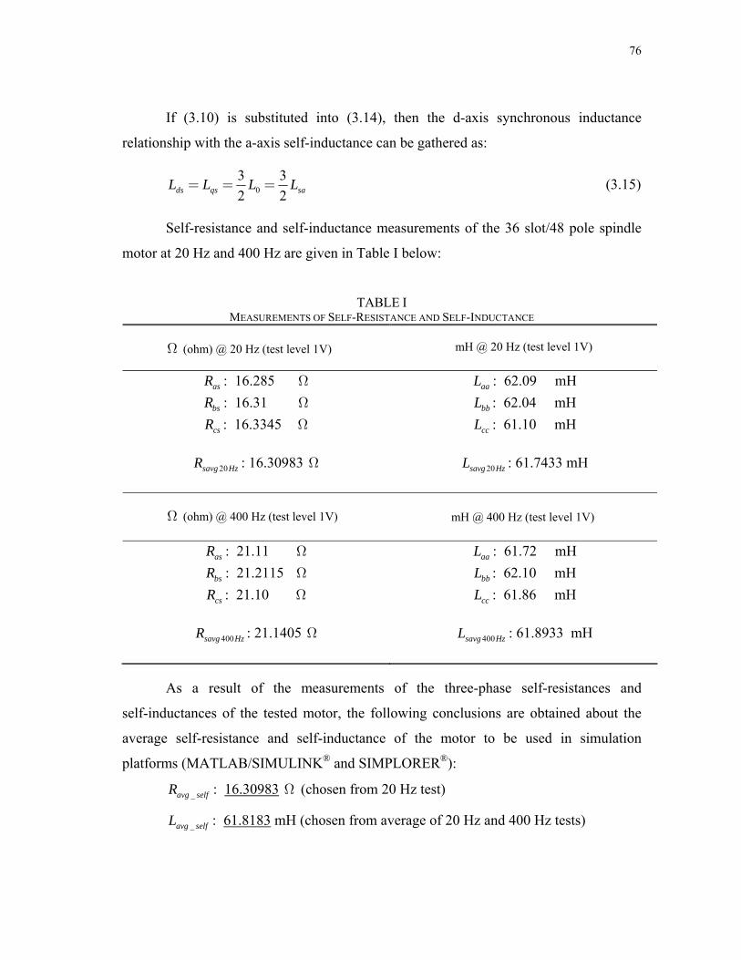
76
If (3.10) is substituted into (3.14), then the d-axis synchronous inductance
relationship with the a-axis self-inductance can be gathered as:
03 32 2ds qs saL L L= = = L (3.15)
Self-resistance and self-inductance measurements of the 36 slot/48 pole spindle
motor at 20 Hz and 400 Hz are given in Table I below:
TABLE I MEASUREMENTS OF SELF-RESISTANCE AND SELF-INDUCTANCE
Ω (ohm) @ 20 Hz (test level 1V)
mH @ 20 Hz (test level 1V)
asR : 16.285 Ω
bsR : 16.31 Ω
csR : 16.3345 Ω
20savg HzR : 16.30983 Ω
aaL : 62.09 mH
bbL : 62.04 mH
ccL : 61.10 mH
20savg HzL : 61.7433 mH
Ω (ohm) @ 400 Hz (test level 1V)
mH @ 400 Hz (test level 1V)
asR : 21.11 Ω
bsR : 21.2115 Ω
csR : 21.10 Ω
400savg HzR : 21.1405 Ω
aaL : 61.72 mH
bbL : 62.10 mH
ccL : 61.86 mH
400savg HzL : 61.8933 mH
As a result of the measurements of the three-phase self-resistances and
self-inductances of the tested motor, the following conclusions are obtained about the
average self-resistance and self-inductance of the motor to be used in simulation
platforms (MATLAB/SIMULINK® and SIMPLORER®):
_avg selfR : 16.30983 Ω (chosen from 20 Hz test)
_avg selfL : 61.8183 mH (chosen from average of 20 Hz and 400 Hz tests)

77
The synchronous inductance of the motor is obtained using (3.13) and the above
average value of the self-inductance from above as:
3 3 61.8183 92.72745 2 2s ds qs saL L L L= = = = = mH
Although using the LCR meter is an easy way to measure the line-to-line and
line-to-neutral (if the motor has a neutral access) inductances, LCR meters generally use
a test frequency on the order of 1 kHz with very low currents, so the measured
inductance may differ appreciably from the correct value which corresponds to a lower
frequency and much higher currents. A complete experimental analysis of the
inductances requires DC inductance measurements using, for example, the Prescot
bridge described by Jones [17], which can be modified to permit inductances to be
measured with varying levels of bias to demagnetizing stator MMF or quadrature-axis
stator MMF [17].
It is a good idea to take inductance measurements at several rotor positions.
Unless there are some problems with the magnets in the motor, there should be very
little inductance variation observed as the rotor rotates in a surface-mounted PMSM (our
test motor is a surface-mounted PMSM). On the other hand, interior-mounted PMSMs
have a saliency such that inductances vary greatly with the rotor position. When the
d-axis inductance is measured by a locked-rotor test in an interior-mounted PMSM the
q-axis synchronous inductance can be measured if the rotor is rotated 90 mechanical
degrees CCW or CW from the d-axis. The rotor could have been brought to the 90
degree electrical position when the a-axis is chosen as a reference, but if the motor is a
high pole motor such as our test motor, rotating the motor 90 electrical degrees from the
reference position is more difficult than rotating it 90 mechanical degrees.
To get the synchronous inductance of the tested motor more precisely another
method can be performed which does not eliminate the leakage inductance in the
calculations. This technique is applicable if the motor has a neutral access. In this thesis,
this method is not implemented, but the theory behind it will be explained in below:

78
To find the leakage inductance, slL , a line-to-line inductance measurement
should be performed corresponding equation is given by:
2LL sa sb abL L L M= + − (3.16)
where abM is the mutual inductance between Phase A and Phase B. If the system is
symmetrical then all the self-inductances are equal,( ), therefore the
line-to-line inductance can be summarized as:
sa sb scL L L= = = L
2( )LL abL L M= − (3.17)
If the line-to-line inductance is measured between Phase A and Phase B and the
self-inductance measurement result, which is obtained from the previous experiment for
Phase A is placed into (3.17), then the mutual inductance, abM , between Phase A and
Phase B can be found easily.
01 cos 22ab ms rM L L θ=− + (3.18)
Because the dq-axes inductances are the same, the saliency coefficient for mutual
inductances will also be equal to zero and the final mutual inductance equation, without
the term, can be shown as: msL
012abM L=− (3.19)
The self-inductance of Phase A without the term and including leakage
inductance is written as:
msL
0sa slL L L= + (3.20)
Knowing abM and putting it in (3.19), is obtained. If is then substituted in
(3.20), then
0L 0L
slL can be found because saL was known previously from the LCR meter
result which includes the leakage inductance effect also.

79
If the d- and q-axis inductances, sdL and sqL , in (3.12) and (3.13) are re-written
including the known leakage inductance, then we obtain:
03 ( )2ds md ls ms lsL L L L L L= + = + + (3.21)
03 ( )2ds mq ls ms lsL L L L L L= + = − + (3.22)
where all the components in the above equations are known so that the d- and q-axis
inductances, sdL and sqL , can be precisely found.
3.4. Measurement of the Back-EMF Constant ( ) and PM Flux Linkage ( ) ek rλ
To calculate the rotor flux linkage, rλ , which is the line-to-neutral peak rotor flux
linkage amplitude value, first the back-EMF constant, ek , is measured. This done by the
generator test in which the tested motor is coupled to a DC motor and it is driven
through the shaft by the DC motor at a constant mechanical speed, rmω . The flux linkage
of the permanent magnet, rλ , and the peak value of back-EMF constant, ek , can then be
easily obtained by measuring the no load line-to-neutral peak voltage (back-EMF, anpkE )
of the motor while it is driven by DC motor. The derivation of rλ is given by:
2 2 2anpk e re e eE k kω= = fπ (3.23)
If the peak back-EMF constant, 2 ek , is replaced by the line-to-neutral peak
rotor flux linkage value, , in (3.23), we obtain: rλ
2 0.223256 /anpkr e
re
Ek Vλ
ω= = = rad s (3.24)

80
where 2re rmP
ω ω= ; is the number of poles and is the mechanical speed in
rad/sec.
P rmω
When the motor has no neutral access, the measurement of the peak
line-to-neutral back-EMF, anpkE , is impossible. In this case, the following procedures
need to be conducted to find the peak rotor flux amplitude, : rλ
First, the line-to-line and line-to-neutral voltage relation is written as:
3ab anV = V (3.25)
The relationship between the rms and peak voltages can be expressed as:
2pk rmsV V= (3.26)
The measured line-to-line rms value of the back-EMF is equal to:
abrms e reE k ω= (3.27)
where is the line-to-line back-EMF constant. From (3.25), the back-EMF is
considered as a voltage, therefore:
ek
3ab
anEE = (3.28)
The peak value of (3.27) is given by:
2abpk e reE k ω= (3.29)
If (3.29) is substituted into (3.28), we obtain:
23
eanpk re
kE ω= (3.30)
Equation (3.30) is the placed into (3.24) and the following result is gathered.
2 2 23 3
anpk abpkr
re rm
E Ek
Pλ
ω ω= = = e (3.31)

81
TABLE II MEASUREMENTS OF LINE-TO-NEUTRAL BACK-EMF FOR EACH PHASE (0-50 RPM)
Ean (V-rms) Ebn (V-rms) Ecn (V-rms) freq-Ea(Hz) speed(RPM)0 0 0 0 0
4.417 4.467 4.68 4.56 11.34.397 4.513 4.648 4.52 11.34.321 4.33 4.524 4.38 11.34.384 4.514 4.626 4.53 11.38.2 8.159 8.348 8.3 20.8
8.256 8.207 8.429 8.31 20.88.24 8.216 8.41 8.34 20.87.993 8.58 8.396 8.35 20.811.701 11.887 12.106 12.03 30.411.914 12.038 12.211 12.18 30.411.996 12.119 12.243 12.25 30.412.04 12.17 12.31 12.19 30.416.34 16.28 15.75 16.15 40.216.28 16.25 15.71 16.18 40.216.25 16.25 15.7 16.14 40.216.08 16.11 15.58 15.96 40.215.56 16.3 16.3 16.15 40.215.53 16.27 16.31 16.11 40.219.67 19.79 19.65 19.85 5019.91 19.88 19.9 20.05 5019.91 19.88 19.9 20.04 5019.92 19.9 19.94 20.08 50
If the average value of the line-to-neutral back-EMF, , found in Table II,
is substituted into (3.23), then the average back-EMF constant, , can be derived as:
anpkavgE
ek
ek =0.223256 Vrad/s
3.5. Load Angle (δ ) Measurement
Load angle measurement is performed in this thesis to validate the motor model
in the simulations by making the motor model as similar to the real motor as possible.

82
δ , is the angle between the back-EMF,Load angle, E , and the input voltage of the
same phase back-EMF, V , as shown in Fig. 3.1.
To measure the load angle, the following equipment is used:
1) Three-phase AC power source
2) LeCroy Digital Storage Oscilloscope (DSO)
3) Maxtrol Hysteresis Dynamometer (max torque is 11.3 lbs)
4) Hall-effect sensor mounted on the stator
Back-EMF (Phase-A)
Hall-Effect Signal (Phase-A)
0δ =ωt
Fig. 3.3. Phase A voltage waveform and hall-effect signal of the same phase.
A load angle measurement is conducted for Phase A of the tested motor. It could
have been performed for the other phases, but under symmetrical conditions the results
would be the same. For the motor that it is used in this thesis, the line-to-neutral
back-EMF is aligned with the corresponding hall-effect signal so that hall-effect sensor
signals are used to get the back-EMF, E , position. The load angle will be the angle of
back-EMF, E , with respect to the input voltage of the same phase back-EMF, V . A
difficulty that exists though is reading the hall-effect signals on the oscilloscope
efficiently. This is due to jittering in the hall-effect signals. The reason this jittering
occurs is because of uneven distribution of the magnets on the rotor. Whenever the N
pole is seen by the hall-effect sensor it generates a pulse, and when the S pole is seen the
signal goes to zero. Fig. 3.4 shows an example of uneven distribution of the magnets
causing jittering in the hall-effect signals:

83
N SN S N S
15 V
0V
24 magnets in one electrical revolution.
Hall-effect signals
Time(s)
Fig. 3.4. Rotor magnet representation along with hall-effect signals.
From the above figure, it can be observed that uneven distribution of the magnets
alters the width of the hall-effect signals and causes jittering in the running motor as
mimicked in the graph below:
Back-EMF (Phase-A)
Hall-Effect Signal (Phase-A)
δ is not exactly zero because of jittering.
? t
Fig. 3.5. Phase A voltage waveform and hall-effect signal with jittering effect.
As it can be seen in Fig. 3.5, uneven distribution of the magnets on the rotor
causes shaking back and forth in hall-effect signals creating difficulty in reading those
signals on the oscilloscope. To overcome the jittering problem (not %100), The LeCroy
DSO is used to average 20 pulses of the hall-effect signal for Phase A, . aH
There are two different ways of measuring the load angle which are explained
below:

84
1) The motor is started and operated in open-loop by a three-phase AC power
supply. When V / f control is used starting from V / f = 1 (20 Vrms) up to 2
(40 Vrms) for a reference test frequency at 20 Hz, when operating frequency is
chosen as 40 Hz (100 rpm) using V / f ~= 1 (40 Vrms) created an unbalance
operation of the motor such that over 30 Hz the motor oscillates a lot (very
unbalanced current is observed after 25-30 Hz with V / f ~= 1). To diminish the
oscillation, the motor should have had a higher current flow through them over
the 25-30 Hz frequencies. In this case V / f ~= 2 is chosen which means there is
an 80 Vrms input sine wave applied to handle up to 10 N·m of load torque at
100 rpm (40 Hz). V / f ~= 2 is chosen as our operating point for most of the
tests to achieve less oscillation in the current, speed and torque response. The
results for the 40 Hz test frequency under no-load but with an increased applied
voltage condition is shown in Fig. 3.7.
The three-phase AC power supply is a programmable AC source such that
various voltage and frequency levels as well as steps in either can be preset. For
example, in the load test the motor is started at a low frequency, such as 12 Hz to
15 Hz, and then the frequency is automatically increased to the desired test level
(20 Hz and 40 Hz).
The applied voltage, V , is then increased from 20 Vrms up to 40 Vrms for the
first part of the load test (the second part starts from 70 Vrms and up to
90 Vrms). The voltage is incremented by 5 Vrms at the test frequency. At each
increment the average of the hall-effect signal is read on the DSO. The DSO then
calculates the load angle between the applied voltage and its corresponding hall-
effect signal. When the applied voltage is increased, the load angle increases
simultaneously, shown in the vector phasor diagram of the PMSM in Fig. 3.9.
When the applied voltage, sV , is increased, the current, sI , also increases so that
the sV vector moves farther than corresponding back-EMF, thus the load angle

85
increases. Related results to the first measurement technique are shown in
Figs. 3.6 and 3.7.
2) The above procedures are applied to the second part of the load test in which
motor is started under open-loop conditions as discussed before up to a 40 Hz
operating frequency with V / f =~ 2 (80 Vrms). When the motor reaches 40 Hz,
a load torque is applied from zero up to 10 N·m by the dynamometer. The results
are obtained as a graph shown in Fig. 3.8. When the motor is loaded, the current
flows through the terminal conductors to the motor and the applied voltage
deviates from the corresponding back-EMF so that the load angle is generated.
With the phase (radian) function and reasonable sweeping (25-100 sweeps), the
load angle, δ , values are collected for various operation points and are shown in the
figure below:
Experimental vs. Simulation Load Angle (deg) @ 20Hz Under No-Load(Ld=Lq=92.7274mH)
0
5
10
15
20
25
30
35
20 25 30 35 40 45
Applied voltage (RMS)
Delta
(deg
)
delta.exp delta.sim
Fig. 3.6. Experimental vs. simulated load angle (deg.) at 20 Hz (No-load).

86
Experimental vs. Simulation Load Angle (deg) @ 40Hz Under No-Load (
0.
5.
10.
15.
20.
25.
70 75 8 85 90
Delta
(eg
)
Ld=Lq=92.7274mH)
25
25
25
25
25
25
0 95
Applied voltage (RMS)
ddelta.exp delta.sim
Fig. 3.7. Experimental vs. simulated load angle (deg.) at 40 Hz (No-load).
Experimental vs. Simulation Load Angle (deg) @ 40Hz Under Load (Ld=Lq=92.7274mH)
-10
-5
0
5
10
delta.sim delta.exp Linear (delta.exp)
15
20
0 1 2 3 4 5 6 7 8 9 10 11
Load Torque (Nm)
Del
ta (d
eg)
Fig. 3.8. Experimental vs. simulated load angle (deg.) at 40 Hz (Load).
The reason we compared the load angles of both the simulation and experiment is
that for the same rms value of the motor current ( ), the behavior of the overall system
is different. This is because of the possible difference between the parameters of the
sI

87
motor model and the real motor. The overall behavior of the PMSM system is shown in
the graph below:
δ
d-axis
q-axis
s sI R
E
s sjI X
V
sIϕ
δ′
V
sI
Fig. 3.9. Possible vector representation of PMSM.
It can be shown from Fig. 3.9 that even if the amplitude of sI is same, the
difference in position of sI will affect the behavior of PMSM. That is why load angle
values from both the simulation and the experiment are compared.

88
CHAPTER IV
OPEN-LOOP SIMULINK® MODEL OF THE PM SPINDLE MOTOR
4.1. Principles of PMSM Open-Loop Control
When the stator resistance, sR , is neglected (near the motor base speed ), the
torque expression for non-salient (surface-mounted PMSM) is given in (5.7), referred to
as (4.1):
bω
3 s2em
e s
PTX
δω
⎛ ⎞⎟⎜= ⎟⎜ ⎟⎜⎝ ⎠sV E
in Equation Section 4(4.1)
where is the variable angular frequency, 2eω efπ , of the input AC supply to the motor,
sV is the rms AC supply voltage of the motor at frequency ef and sX is the synchronous
reactance, 2 e sf Lπ , of the motor at the supply frequency.
Since the back-EMF, E , and the synchronous reactance, sX , are proportional to
the angular frequency , then the same maximum torque (when ) is achieved if
the
eω 90δ =
s
e
Vω
or s
e
Vf
ratio is maintained constant at all speeds (frequencies) at a given load
angle . This control method is very similar to the one used for induction motors. The
above methodology used as an open-loop control for PMSM drives is valid when the
motor speed is near the base speed (or base frequency). This is because near base speed
the back-EMF of the motor,
δ
E , and supply voltage, sV , are much larger than the voltage
drop in the stator resistance. On the other hand, at low frequencies the voltage drop due
to the stator resistance may not be negligible.

89
In open-loop control ( /V f control) the speed of the motor is commanded by the
input frequency ef of the supply, and sV is chosen such that at all speeds /V f is
maintained constant so as not to strengthen the stator flux linkage more than its normal
value. To implement the idea of /V f control, a sinusoidal PWM technique can be used.
Sudden reference speed changes may cause load angle to exceed its limit (=90 ) as a
precaution, a filter in the speed reference input may be used, as shown in Fig. 4.1.
Generally,
δ
sV is increased proportionally with ef until base frequency is reached.
Afterwards, the constant torque region ends and field weakening region, or constant
power region, is started. In that region sV is maintained constant at the base voltage, ,
of the motor providing constant power. Above the base speed, , only the supply
frequency
bV
bω
ef can be increased which weakens the stator flux linkage so that maximum
torque is reduced according to (5.7).
PMSM
A
B
C
ef
bV
bfsV
11 fT s+
t
Speed filterto avoid suddenspeed change
Speedreference
referencesV
referenceef
SPWMVSI
Fig. 4.1. Basic open-loop block diagram of PMSM.

90
4.2. Building Open-Loop Steady and Transient-State Models
Even though the conventional washing machine agitation speed control system is
simulated in the SIMPLORER® platform, open-loop steady state and even transient
controls are done in MATLAB/SIMULINK® because steady-state motor models are not
provided in SIMPLORER®. The ones it provides are transient models, and modification
of the models is not allowed. Therefore, relying on the convenience of SIMULINK®,
open-loop, steady-state and transient models are built in the MATLAB/SIMULINK®
platform. The dq-rotor model equations used in the open-loop control of the PMSM are
written again:
( )
( )q s s q r s d r
d s s d r s q
v R L p i L i
v R L p i L i
ω ω
ω
= + + +
= + −rλ
rλ
(4.2)
where is the derivative. p
If the derivative terms are removed, the steady-state voltage equations in the
rotor reference frame become:
q s q r s d r
d s d r s q
v R i L i
v R i L i
ω ω
ω
= + +
= − (4.3)
Fig. 4.2 is the block diagram of the overall open-loop PMSM drive system
designed in MATLAB/SIMULINK®. In this figure, transformations are in the following
order from left to right: abc reference frame to -stationary reference frame
transformation, -stationary reference frame to dq-rotor reference frame
transformation and finally dq-rotor reference frame to abc-frame transformation.
DQ
DQ

91
mean(VI.signals.values)/(80*max(ialoaded.signals.values)/sqrt(2))
For cos (Phi)
((mean(P.signals.values))/(24))/((3*80*max(ialoaded.signals.values)/sqrt(2))*(mean(VI.signals.values)/(80*max(ialoaded.signals.values)/sqrt(2))))For eff.
w m_rpm
-K-
w e_to_w mvc
vb
va
qdr2abc
ia
delta
abc2qd1
VI
Tem
Scope10
Product1
Product
f(u)
Pf=P/S
Pactive
PF
P
Load Torque1
PM-SM
idiq
Temwr_sliptheta_e
phi_dphi_q
wrdelta
F&P BPMmotor model
emVabc
IabcPQ
3-phase Instantaneous
Active & Reactive Pow er
vds
abc2qd0qds2qdr
vqs
2
vqr
1
vdr
u[1]*u[3] - u[2]*u[4]
qds2qr
u[2]*u[3] + u[1]*u[4]
qds2dr
(2*u[1]- u[2] - u[3])/3
abc2q
(u[3] -u[2])/sqrt(3)
abc2d
Mux
Mux1Mux
Mux
sin(u)
Fcn1
cos(u)
Fcn4
thetar
3
vc
2
vb
1
va
Fig. 4.2. Overall open-loop control block diagram of PMSM in SIMULINK®.
Fig. 4.3. Abc to stationary and stationary to dq rotor reference frame transformation
block.
where and or and are the stationary reference frame voltages converted
from the motors abc terminal voltages by using Clark’s Transformation which are given
by:
qsv dsv vα vβ

92
(2 )3
( )3
a b cqs
c bds
v v vv v
v vv v
α
β
− −= =
−= =
(4.4)
From Fig. 4.3, the stationary to rotor reference frame voltage equations
corresponding to the Park’s Transformation under the assumption that the rotor angle
representation is chosen between the rotor q-axis and the stationary q-axis, as shown in
Fig. 4.4, are given by:
cos sin
sin cos
s sq q r d
s sd q r d
v v v
v v v
θ θ
θ θ
= −
= +
r
r
(4.5)
The coordinate representation of the stationary reference frame is shown in
Fig. 4.4.
sq
sd
rd
rq
rθ
rθ
Fig. 4.4. Rotor reference frame and stationary reference frame coordinate representation.

93
qdr2qdsqds2abc
3
ic
2
ib
1
ia
-u[1]/2 +sqrt(3)*u[2]/2
qds2c
-u[1]/2 -sqrt(3)*u[2]/2
qds2b
u[1]
qds2au[1]*u[3] + u[2]*u[4]
qdr2qs
u[1]*u[4] - u[2]*u[3]
qdr2ds
Mux
Mux1
Mux
Mux
sin(u)
Fcn1
cos(u)
Fcn3
thetar
2
iq
1
id
Fig. 4.5. Dq rotor reference frame to stationary and stationary to abc transformation
block.
From Fig. 4.5, the rotor frame to stationary frame current equations
corresponding to the inverse Park’s Transformation, under the assumption that the rotor
angle representation is chosen as between the rotor q-axis and the stationary q-axis as
shown in Fig. 4.4, are given by:
cos sin
cos sin
sq q r d
sd d r q
i i i
i i i
θ θ
θ θ
= +
= −
r
r
(4.6)
Again from Fig. 4.5, the stationary frame to the abc frame current transformation
corresponding to the inverse Clark’s Transformation can be expressed as:
1 32 21 32 2
a qs
b qs
c qs
i i
i i
i i
=
=− −
=− +
ds
ds
i
i
(4.7)
From Fig. 4.2, the inside of the PMSM model is presented in Fig. 4.6.

94
wr
Vd
Vq
id
iq
wr_slip
electrical_pos.
9
delta
8
wr
7
out_7
6
out_6
5
out_5
4
out_4
3
out_3
2
out_2
1
out_1
0
wr=0 if wr<0
p/J
p/J
we
lPM1
Lamdam
lPM
Lamdam
lPM
1
RsTransfer Fcn1,Lq
1
RsTransfer Fcn,Ld
Switch
Sum5
Sum4
Sum3
Sum2
Sum1
Sum
Product2
Product1
Product
LqLq
Lq
Lq
-K-
Ld-Lq
Ld
Ld
1/s
Integrator1
1/s
Integrator
1/s
Integrator
-K-
1.5*p
3
in_3
2
in_2
1
in_1
Fig. 4.6. Steady state dq-axis rotor reference frame motor model.
Equations for Fig. 4.6 can be summarized as:

95
3 ( ( ) )2 2
( ( ) ) ( )2
q s q r d d r r
d s d r q q
em i q d q q d
r e rmem mech damp
v R i L i
v R i L i
PT i L L i i
d t tJT T T JP dt dt
ω ω λ
ω
λ
ω ω ω
= + +
= −
= + −
−+ − = =
(4.8)
where damping torque, , is assumed to be zero. dampT
0
0
( ) ( ) ( )
( ) (0) (0)
( ( ) ) ( )
( ) ( )2
r e
t
r e r e
r e r
t
r e em mech damp
t t t
t dt
d t d tdt dt
Pt T T TJ
δ θ θ
ω ω θ θ
ω ω ω
ω ω
= −
= − + −
−=
− = + −
∫
∫ dt
(4.9)
where is the initial value of the load angle, , also known as ‘delto’ in
the simulation.
(0) (0)r eθ θ− (0)δ
When the steady-state rotor speed is equal to the synchronous speed er t ωω =)( ,
δ (load angle) is constant and 0=rslipω ( 0)( =− er t ωω ). It is always better to get
0)0( =eθ . This is done by aligning the d-axis (synchronous reference frame) with the
a-axis or stationary reference frame as shown in Fig. 4.7.

96
δ
rθ eθ
rq
axisaqs
,
eq
−
eq sq
Fig. 4.7. Rotor ref. frame, synchronous ref. frame, and stationary ref. frame
representation as vectors.
For ease the -axis will also be aligned with the a-axis which makes the rotor
initial position zero (we need to be aware of this in the experiment also). If the
SIMULINK
rq
® open-loop control is used in the transient analysis, then the synchronous
speed, , is chosen to be zero because the initial speed of the rotor is zero in the
beginning of transient-state. In steady-state the desired speed is 2*pi*40 electrical rad/s
for 100 rpm (48 rotor poles). Additionally, (4.3) is used for designing the transient
PMSM model instead of (4.2).
eω
For the correct load angle in the SIMULINK® model, the ‘delto’ value in the
motor model should be equal to pi/2 for the following reason:
Let’s assume that the input voltage waveform is ))0(cos( eema tVV θω += (our
input is a sine wave), which means 0)0( =eθ . If )0(eθ is not zero (as with a sine wave
excitation of )sin( tVV ema ω= (like the model used in SIMULINK®) which equals
)2/cos( πω −tV em where 2/)0( πθ −=e ), the no-load steady-state value of δ will be
2/π− instead of zero, therefore ‘delto’ will be 2/π [10].

97
4.3. Power Factor and Efficiency Calculations in Open-Loop Matlab/Simulink®
Model
To verify that the simulated model is exactly like the real motor more
characterization tests should be conducted, such as power factor and efficiency
comparisons. These can be calculated in the MATLAB/SIMULINK® platform in two
ways. One way is by using SIMULINK® internal power measurement blocks. The other
way to obtain these is by using the MATLAB® workspace with the following equations:
cose _cos_
( . . )max( . . )80
2
rms rms
rms rms
rms rms
V IR al Power PPFApparent Power S V I
P mean VI signals valuesia signals valuesS V I
φφ= = = =
=⎛ ⎞⎟⎜= = ⎟⎜ ⎟⎟⎜⎝ ⎠
(4.10)
where is the abbreviation for Power Factor, is the apparent power, and 80 is the
rms value of the applied sinewave voltage.
PF S
P is calculated by taking the average (mean function) of VI which is the product
of (phase A voltage) and (phase A current). They are shown as the scope names in
SIMULINK
av ai® shown in Fig. 4.2. Below is the derivation of the efficiency formula which
is used in MATLAB®:
;3 cos 2
( )/ 2
3 cos
out em me m
in rms rms
eem
rms rms
P T PP V I
TP
V I
ωη ω
φ
ω
ηφ
= = =
=
ω
(4.11)
where φ is the power factor angle between the motor voltage and current.
The formulas below are used to calculate the power factor and efficiency. They
are used in MATLAB® workspace after the simulation ends:
Power Factor (PF):
mean(VI.signals.values)/(80*max(ia.signals.values)/sqrt(2))
98
Motor Efficiency (Eff.):
((mean(P.signals.values))/(24))/((3*80*max(ia.signals.values)/sqrt(2))*
(mean(VI.signals.values)/(80*max(ia.signals.values)/sqrt(2))))
In open-loop steady-state control there is a transient in the beginning, so to have
the real values data should be collected when transient passes, otherwise the transient
will dramatically change the PF and eff. values. To do that, in the scope parameters the
‘limit data points to last’ description should be sufficient enough to pass and not include
those transient effects. For example, 5000 points is chosen in the simulation and that was
enough for the calculation of PF and eff. Once the simulation is run the signal values
which are collected from the SIMULINK® scopes are run in the MATLAB® workspace
using the equations above so that the PF and eff. values are obtained. Similarly, the
SIMULINK® internal Power Measurement blocks can be used to calculate the PF and
Active (Real) Power easily. With those results, the eff. block can also be built in
SIMULINK®, as given below:
( )24
e
out
in active
P scopePP P
η= = (4.12)
where 24 is the pole pair number of the 48 pole PM spindle motor, is the
electrical output power of the motor and is the resultant active power part of the
output of the built-in internal power block. If better power results are desired then they
can be averaged out using ‘mean (P.signals.values)’, but it can only be done in the
MATLAB
( )eP scope
activeP
® command screen.

99
CHAPTER V
CONVENTIONAL DIRECT TORQUE CONTROL (DTC)
OPERATION OF PMSM DRIVE
5.1. Introduction and Literature Review
Today there are basically two types of instantaneous electromagnetic
torque-controlled AC drives used for high-performance applications: vector and direct
torque control (DTC) drives. The most popular method, vector control was introduced
more than 25 years ago in Germany by Hasse [18], Blaske [13], and Leonhard. The
vector control method, also called Field Oriented Control (FOC) transforms the motor
equations into a coordinate system that rotates in synchronism with the rotor flux vector.
Under a constant rotor flux amplitude there is a linear relationship between the control
variables and the torque. Transforming the AC motor equations into field coordinates
makes the FOC method resemble the decoupled torque production in a separately
excited DC motor. Over the years, FOC drives have achieved a high degree of maturity
in a wide range of applications. They have established a substantial world wide market
which continues to increase [6].
No later than 20 years ago, when there was still a trend toward standardization of
control systems based on the FOC method, direct torque control was introduced in Japan
by Takahashi and Nagochi [19] and also in Germany by Depenbrock [20], [21], [22].
Their innovative studies depart from the idea of coordinate transformation and the
analogy with DC motor control. These innovators proposed a method that relies on a
bang-bang control instead of a decoupling control which is the characteristic of vector
control. Their technique (bang-bang control) works very well with the on-off operation
of inverter semiconductor power devices.
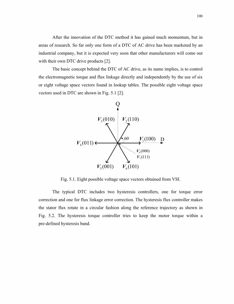
100
After the innovation of the DTC method it has gained much momentum, but in
areas of research. So far only one form of a DTC of AC drive has been marketed by an
industrial company, but it is expected very soon that other manufacturers will come out
with their own DTC drive products [2].
The basic concept behind the DTC of AC drive, as its name implies, is to control
the electromagnetic torque and flux linkage directly and independently by the use of six
or eight voltage space vectors found in lookup tables. The possible eight voltage space
vectors used in DTC are shown in Fig. 5.1 [2].
D
Q
60
6 (101)V
1(100)V
2 (110)V3 (010)V
4 (011)V
5 (001)V
0 (000)V
7 (111)V
Fig. 5.1. Eight possible voltage space vectors obtained from VSI.
The typical DTC includes two hysteresis controllers, one for torque error
correction and one for flux linkage error correction. The hysteresis flux controller makes
the stator flux rotate in a circular fashion along the reference trajectory as shown in
Fig. 5.2. The hysteresis torque controller tries to keep the motor torque within a
pre-defined hysteresis band.

101
D
Q
2θ
1θ
6θ5V 6V
3V 2V
4V1V
1V
2V
3V
1V
2V
3V4
V3
V4V
5V
4V
5V
6V
5V
6V
6V
1V
2V
3θ
4θ
5θ
Fig. 5.2. Circular trajectory of stator flux linkage in the stationary DQ-plane.
At every sampling time the voltage vector selection block decides on one of the
six possible inverter switching states ( , , ) to be applied to the motor terminals.
The possible outputs of the hysteresis controller and the possible number of switching
states in the inverter are finite, so a look-up table can be constructed to choose the
appropriate switching state of the inverter. This selection is a result of both the outputs
of the hysteresis controllers and the sector of the stator flux vector in the circular
trajectory.
aS S Sb c
There are many advantages of direct torque control over other high-performance
torque control systems such as vector control. Some of these are summarized as follows:
• The only parameter that is required is stator resistance

102
• The switching commands of the inverter are derived from a look-up
table, simplifying the control system and also decreasing the processing
time unlike a PWM modulator used in vector control
• Instead of current control loops, stator flux linkage vector and torque
estimation are required so that simple hysteresis controllers are used for
torque and stator flux linkage control
• Vector transformation is not applied because stator quantities are enough
to calculate the torque and stator flux linkage as feedback quantities to be
compared with the reference values
• The rotor position, which is essential for torque control in a vector
control scheme, is not required in DTC (for induction and synchronous
reluctance motor DTC drives)
Once the initial position of the rotor magnetic flux problem is solved for PMSM
drives by some initial rotor position estimation techniques or by bringing the rotor to the
known position, DTC of the PMSM can be as attractive as DTC of an induction motor. It
is also easier to implement and as cost-effective (no position sensor is required) when
compared to vector controlled PMSM drives. The DTC scheme, as its name indicates, is
focused on the control of the torque and the stator flux linkage of the motor, therefore, a
faster torque response is achieved over vector control. Furthermore, due to the fact that
DTC does not need current controller, the time delay caused by the current loop is
eliminated.
Even though the DTC technique was originally proposed for the induction
machine drive in the late 1980’s, its concept has been extended to the other types of AC
machine drives recently, such as switched reluctance and synchronous reluctance
machines. In the late 90s, DTC techniques for the interior permanent magnet
synchronous machine appeared, as reported in [23], [24].
Although there are several advantages of the DTC scheme over vector control, it
still has a few drawbacks which are explained below:
103
• A major drawback of the DTC scheme is the high torque and stator flux
linkage ripples. Since the switching state of the inverter is updated once
every sampling time, the inverter keeps the same state until the outputs of
each hysteresis controller changes states. As a result, large ripples in
torque and stator flux linkage occur.
• The switching frequency varies with load torque, rotor speed and the
bandwidth of the two hysteresis controllers.
• Stator flux estimation is achieved by integrating the difference between
the input voltage and the voltage drop across the stator resistance (by the
back-EMF integration as given in (5.9)). The applied voltage on the
motor terminal can be obtained either by using a DC-link voltage sensor,
or two voltage sensors connected to the any two phases of the motor
terminals. For current sensing there should be two current sensors
connected on any two phases of the motor terminals. Offset in the
measurements of DC-link voltage and the stator currents might happen,
because for current and voltage sensing, however, temperature sensitive
devices, such as operational amplifiers, are normally used which can
introduce an unwanted DC offset. This offset may introduce large drifts
in the stator flux linkage computation (estimation) thus creating an error
in torque estimation (torque is proportional to the flux value) which can
make the system become unstable.
• The stator flux linkage estimation has a stator resistance, so any variation
in the stator resistance introduces error in the stator flux linkage
computation, especially at low frequencies. If the magnitude of the
applied voltage and back-EMF are low, then any change in the resistance
will greatly affect the integration of the back-EMF.
• Because of the constant energy provided from the permanent magnet on
the rotor the rotor position of motor will not necessarily be zero at start
up. To successfully start the motor under the DTC scheme from any

104
position (without locking the motor at a known position), the initial
position of the rotor magnetic flux must be known. Once it is started
properly, however, the complete DTC scheme does not explicitly require
a position sensor.
From the time the DTC scheme was discovered for AC motor drives, it was
always inferior to vector control because of the disadvantages associated with it. The
goal is to bring this technology as close to the performance level of vector control and
even exceed it while keeping its simple control strategy and cost-effectiveness. As a
result, many papers have been presented by several researchers to minimize or overcome
the drawbacks of the DTC scheme. Here are some of the works that have been done by
researchers to overcome the drawbacks for the most recent AC drive technology using
direct torque control:
• Recently, researchers have been working on the torque and flux ripple
reduction, and fixing the switching frequency of the DTC system, as
reported in [25]-[30]. Additionally, they came up with a multilevel
inverter solution in which there are more voltage space vectors available
to control the flux and torque. As a consequence, smoother torque can be
obtained, as reported in [28] and [29], but by doing so, more power
switches are required to achieve a lower ripple and an almost fixed
switching frequency, which increases the system cost and complexity. In
the literature, a modified DTC scheme with fixed switching frequency
and low torque and flux ripple was introduced in [27] and [30]. With this
design, however, two PI regulators are required to control the flux and
torque and they need to be tuned properly. Very recently Rahman [31]
proposed a method for torque and flux ripple reduction in interior
permanent magnet synchronous machines under an almost fixed
switching frequency without using any additional regulators. This method
is a modified version of the previously discovered method for the
induction machine by the authors in [32].
105
• Stator flux linkage estimation by the integration of the back-EMF should
be reset regularly to reduce the effect of the DC offset error. There has
been a few compensation techniques related to this phenomenon proposed
in the literature [33]-[35] and [16]. Chapuis et al. [18] introduced a
technique to eliminate the DC offset, but a constant level of DC offset is
assumed which is usually not the case. In papers [33]-[35] and [16],
low-pass filters (LPFs) have been introduced to estimate the stator flux
linkage. In [33], a programmable cascaded LPF was proposed instead of
the single-stage integrator to help decrease the DC offset error more than
the single-stage integrator for induction motor drives. More recently,
Rahman [36] has reached an approach like [33] with further investigation
and implementation for the compensation of DC offset error in a direct
controlled interior permanent magnet (IPM) synchronous motor drive. It
has been claimed and proven with simulation and experimental results
that programmable cascaded LPFs can also be adopted to replace the
single-stage integrator and compensate for the effect of DC offsets in a
direct-torque-controlled IPM synchronous motor drive, improving the
performance of the drive.
• The voltage drop in the stator resistance is very large when the motor runs
at low frequency such that any small deviations in stator resistance from
the one used in the estimation of the stator flux linkage creates large
errors between the reference and actual stator flux linkage vector. This
also affects the torque estimation as well. Due to these errors, the drive
can easily go unstable when operating at low speeds. The worst case
scenario might happen at low speed under a very high load. A handful of
researchers have recently pointed to the issue of stator resistance variation
for the induction machine. For example, fuzzy and proportional-integral
(PI) stator resistance estimators have been developed and compared for a
DTC induction machine based on the error between the reference current

106
and the actual one by Mir et al. [37]. On the other hand, they did not show
any detail on how to obtain the reference current for the stator resistance
estimation. Additionally, some stability problems of the fuzzy estimator
were observed when the torque reference value was small. As reported in
[38], fuzzy logic based stator resistance observers are introduced for
induction motor. Even though it is an open-loop controller based on fuzzy
rules, the accuracy of estimating the stator resistance is about 5% and
many fuzzy rules are necessary. This resulted in having to conduct
handful numbers of extensive experiments to create the fuzzy rules
resulting in difficulty in implementation. Lee and Krishnan [39]
contributed a work related to the stator resistance estimation of the DTC
induction motor drive by a PI regulator. An instability issue caused by the
stator estimation error in the stator resistance, the mathematical
relationships between stator current, torque and flux commands, and the
machine parameters are also analyzed in their work. The stator
configuration of all AC machines is almost the same, so the stator
resistance variation problem still exists for permanent magnet
synchronous motors. Rahman et al. [40] reported a method, for stator
resistance estimation by PI regulation based on the error in flux linkage. It
is claimed that any variation in the stator resistance of the PM
synchronous machine will cause a change in the amplitude of the actual
flux linkage. A PI controller works in parallel with the hysteresis flux
controller of the DTC such that it tracks the stator resistance by
eliminating the error in the command and the actual flux linkage. One
problem with this method was that the rotor position was necessary to
calculate the flux linkage. Later on the same author proposed a similar
method but this time the PI stator resistance estimator was able to track
the change of the stator resistance without requiring any position
information.

107
• The back-EMF integration for the stator flux linkage calculation, which
runs continuously, requires a knowledge of the initial stator flux position,
0tsλ =, at start up. In order to start the motor without going in the wrong
direction, assuming the stator current is zero at the start, only the rotor
magnetic flux linkage should be considered as an initial flux linkage
value in the integration formula. The next step is to find its position in the
circular trajectory. The initial position of the rotor is not desired to be
sensed by position sensors due to their cost and bulky characteristics,
therefore some sort of initial position sensing methods are required for
permanent magnet synchronous motor DTC applications. A number of
works, [41]-[52], have been proposed recently for the detection of the
initial rotor position estimation at standstill for different types of PM
motors. Common problems of these methods include: most of them fail at
standstill because the rotor magnet does not induce any voltage, so no
information of the magnetization is available; position estimation is load
dependent; excessive computation and hardware are required; instead of a
simple voltage vector selection method used in the DTC scheme, those
estimation techniques need one or more pulse width-modulation (PWM)
current controllers. Recently, a better solution was introduced for the
rotor position estimation. It is accomplished by applying high-frequency
voltage to the motor, as reported in [50]-[52]. This approach is adapted to
the DTC of interior permanent magnet motors for initial position
estimation by Rahman et. al. [36].
5.2. Principles of Conventional DTC of PMSM Drive
The basic idea of direct torque control is to choose the appropriate stator voltage
vector out of eight possible inverter states (according to the difference between the

108
reference and actual torque and flux linkage) so that the stator flux linkage vector rotates
along the stator reference frame (DQ frame) trajectory and produces the desired torque.
The torque control strategy in the direct torque control of a PM synchronous motor is
explained in Section 5.2.1. The flux control is discussed following the torque control
section.
5.2.1. Torque Control Strategy in DTC of PMSM Drive
Before going through the control principles of DTC for PMSMs, an expression
for the torque as a function of the stator and rotor flux will be developed. The torque
equation used for DTC of PMSM drives can be derived from the phasor diagram of
conventional or permanent magnet synchronous motor shown in Fig. 5.3.
δ
d-axis
q-axis
s sI R
E
s sjI X
sV
sIϕ
rλ
Fig. 5.3. Phasor diagram of a non-saliet pole synchronous machine in the motoring
mode.

109
R ss LjjX ω=
°∠0V °∠δfE
Fig. 5.4. Electrical circuit diagram of a non-salient synchronous machine at constant
frequency (speed).
When the machine is loaded through the shaft, the motor will take real power.
The rotor will then fall behind the stator rotating field. From the circuit diagram, shown
in Fig. 5.4, the motor current expression can be written as:
0 0s ss
s s s
V E V EIR jX Z
δϕ
∠ − ∠ ∠ − ∠= =
+ ∠δ (5.1)
where 2 2s s sZ R X= + , also s e sX Lω=
and 1tan s
s
XR
ϕ −⎛ ⎞⎟⎜ ⎟= ⎜ ⎟⎜ ⎟⎜⎝ ⎠
Assuming a reasonable speed such that the sX term is higher than the resistance, sR ,
such that sR can be neglected, then s sZ X≈ and 2π
ϕ≈ . sI can then be rewritten as:
0 2ss
s s
EVIX X
πδ∠ −∠
= − (5.2)
Such that the real part of sI is:

110
Re[ ] cos cos cos2 2
cos sin2
ss s
s s
s s
V EI IX X
E EX X
π πϕ δ
πδ δ
⎛ ⎞ ⎛⎟ ⎟⎜ ⎜= = − − −⎟ ⎟⎜ ⎜⎟ ⎟⎜ ⎜⎝ ⎠ ⎝
⎛ ⎞⎟⎜=− − =−⎟⎜ ⎟⎜⎝ ⎠
⎞⎠
(5.3)
the developed power is given by:
3 Re[ ] 3 cosi s s s sP V I V I ϕ= = (5.4)
Substituting (5.3) into (5.4) yields:
3 sinsi
s
V EPX
δ=− Watts/phase (5.5)
This power is positive when δ negative, meaning that when the rotor field lags
the stator field the machine is operating in the motoring region. When the machine
is operating in the generation region. The negative sign in (5.5) can be dropped,
assuming that for motoring operation a negative δ is implied.
0δ>
If the losses of the machine are ignored, the power can be expressed as the
shaft (output) power as well:
iP
2i o e eP P T
Pω= = m (5.6)
When combining (5.5) and (5.6), the magnitude of the developed torque for a
non-salient synchronous motor (or surface-mounted permanent magnet synchronous
motor) can be expressed as:
3 s2
3 sin2
eme s
s
PTX
PL
δω
δ
⎛ ⎞⎟⎜= ⎟⎜ ⎟⎜⎝ ⎠
⎛ ⎞⎟⎜= ⎟⎜ ⎟⎜⎝ ⎠
s
s r
V E
λ λ
in (5.7)

111
where is the torque angle between flux vectors δ sλ and . If the rotor flux remains
constant and the stator flux is changed incrementally by the stator voltage,
rλ
sV , then the
torque variation, , expression can be written as: emTΔ
32em
s
PTL
δ⎛ ⎞ +⎟⎜Δ = Δ⎟⎜ ⎟⎜⎝ ⎠
s s rλ Δλ λsin (5.8)
where the bold terms in the above expressions indicate vectors.
As it can be seen from (5.8), if the load angle, , is increased then torque
variation is increased. To increase the load angle, δ , the stator flux vector should turn
faster than rotor flux vector. The rotor flux rotation depends on the mechanical speed of
the rotor, so to decrease load angle, δ , the stator flux should turn slower than rotor flux.
Therefore, according to the torque (5.7), the electromagnetic torque can be controlled
effectively by controlling the amplitude and rotational speed of stator flux vector,
δ
sλ . To
achieve the above phenomenon, appropriate voltage vectors are applied to the motor
terminals. For counter-clockwise operation, if the actual torque is smaller than the
reference value, then the voltage vectors that keep the stator flux vector, sλ , rotating in
the same direction are selected. When the load angle, δ , between sλ and increases
the actual torque increases as well. Once the actual torque is greater than the reference
value, the voltage vectors that keep stator flux vector,
rλ
sλ , rotating in the reverse
direction are selected instead of the zero voltage vectors. At the same time, the load
angle, , decreases thus the torque decreases. The reason the zero voltage vector is not
chosen in the DTC of PMSM drives will be discussed later in this chapter. A more
detailed look at the selection of the voltage vectors and their effect on torque and flux
results will be discussed later as well. Referring back to the discussion above, however,
torque is controlled via the stator flux rotation speed, as shown in Fig. 5.5. If the speed
of the stator flux is high then faster torque response is achieved.
δ

112
reωsω
δ
sλ
rλ
Im
Rereθsθ
Fig. 5.5. Rotor and stator flux linkage space vectors (rotor flux lagging stator flux) [35].
5.2.2. Flux Control Strategy in DTC of PMSM Drive
If the resistance term in the stator flux estimation algorithm is neglected, the
variation of the stator flux linkage (incremental flux expression vector) will only depend
on the applied voltage vector as shown in Fig. 5.6 [53].
D
Q
2θ
1θ
6θ
3θ
4θ
5θ
0sλ
sλ∗
2Hλ
3V
2V
4V
3V4V
5V4V
5V
6V
5V
6V
1V6V
1V
2V
2V
2V3V
4V
5V 6V
1V
sλ2 sV T
3V
Fig. 5.6. Incremental stator flux linkage space vector representation in the DQ-plane.

113
For a short interval of time, namely the sampling time, , the stator flux
linkage,
sT =Δt
sλ , position and amplitude can be changed incrementally by applying the stator
voltage vector, sV . As discussed above, the position change of the stator flux linkage
vector, sλ
)
, will affect the torque. The stator flux linkage of a PMSM that is depicted in
the stationary reference frame is written as:
(s s s sR dt= −∫λ V i (5.9)
During the sampling interval time or switching interval, one out of the six
voltage vectors is applied, and each voltage vector applied during the pre-defined
sampling interval is constant, s (5.9) can be rewritten as:
s s s s s t=0t - R dt + λ= ∫λ V i (5.10)
where s t=0λ is the initial stator flux linkage at the instant of switching, Vs is the
measured stator voltage, is , is the measured stator current, and sR is the estimated stator
resistance. When the stator term in stator flux estimation is removed implying that the
end of the stator flux vector, sλ , will move in the direction of the applied voltage vector,
as shown in Fig. 5.6, we obtain:
( )V λs sddt
= (5.11)
or
Δts sΔλ =V (5.12)
The goal of controlling the flux in DTC is to keep its amplitude within a
pre-defined hysteresis band. By applying a required voltage vector stator flux linkage
amplitude can be controlled. To select the voltage vectors for controlling the amplitude
of the stator flux linkage the voltage plane is divided into six regions, as shown in
Fig. 5.2.

114
In each region two adjacent voltage vectors, which give the minimum switching
frequency, are selected to increase or decrease the amplitude of stator flux linkage,
respectively. For example, according to the Table III, when the voltage vector is
applied in Sector 1, then the amplitude of the stator flux increases when the flux vector
rotates counter-clockwise. If is selected then stator flux linkage amplitude decreases.
The stator flux incremental vectors corresponding to each of the six inverter voltage
vectors are shown in Fig. 5.1.
2V
3V
sω
s sTω
sλ
0sλ
Im
Re0sθ
sθ
s sV T
Direct (Flux) component
Indirect (Torque) component
Fig. 5.7. Representation of direct and indirect components of the stator flux linkage
vector [35].
Fig. 5.7 is a basic graph that shows how flux and torque can be changed as a
function of the applied voltage vector. According to the figure, the direct component of
applied voltage vector changes the amplitude of the stator flux linkage and the indirect
component changes the flux rotation speed which changes the torque. If the torque needs
to be changed abruptly then the flux does as well, so the closest voltage vector to the
indirect component vector is applied. If torque change is not required, but flux amplitude
is increased or decreased then the voltage vector closest to the direct component vector
is chosen. Consequently, if both torque and flux are required to change then the
appropriate resultant mid-way voltage vector between the indirect and direct components
is applied [35]. It seems obvious from (5.9) that the stator flux linkage vector will stay at

115
its original position when zero voltage vectors and are applied. This is
true for an induction motor since the stator flux linkage is uniquely determined by the
stator voltage. On the other hand, in the DTC of a PMSM, the situation of applying the
zero voltage vectors is not the same as in induction motors. This is because the stator
flux linkage vector will change even when the zero voltage vectors are selected since the
magnets rotate with the rotor. As a result, the zero voltage vectors are not used for
controlling the stator flux linkage vector in a PMSM. In other words, the stator flux
linkage should always be in motion with respect to the rotor flux linkage vector [24].
(000)S (111)Sa a
5.2.3. Voltage Vector Selection in DTC of PMSM Drive
As discussed before, the stator flux is controlled by properly selected voltage
vectors, and as a result the torque by stator flux rotation. The higher the stator vector
rotation speed the faster torque response is achieved.
The estimation of the stator flux linkage components described previously
requires the stator terminal voltages. In a DTC scheme it is possible to reconstruct those
voltages from the DC-link voltage, , and the switching states ( , , ) of a
six-step voltage-source inverter (VSI) rather than monitoring them from the motor
terminals. The primary voltage vector,
dcV aS bS cS
sv , is defined by the following equation:
(2 /3) (4 /3)2 (3
j js a b cv v e v eπ= + +v )π (5.13)
where , , and are the instantaneous values of the primary line-to-neutral voltages.
When the primary windings are fed by an inverter, as shown in Fig. 5.8, the primary
voltages , and are determined by the status of the three switches, , , and
. If the switch is at state 0 that means the phase is connected to the negative and if it is
at 1 it means that the phase is connected to the positive leg.
av bv cv
av bv cv aS bS
cS

116
aS bS cS1
0
1
0
1
0
dcV
D
Q
Fig. 5.8. Voltage source inverter (VSI) connected to the R-L load [19].
For example, is connected to if is one, otherwise is connected to zero. This
is similar for and . The voltage vectors that are obtained this way are shown in
Fig. 5.1. There are six nonzero voltage vectors: , , …, and and
two zero voltage vectors: and . The six nonzero voltage vectors are
apart from each other as in Fig. 5.1.
av dcV aS av
bv cv
1(100)V 2 (110)V 6 (101)V
7 (000)V 8 (111)V 60
The stator voltage space vector (expressed in the stationary reference frame)
representing the eight voltage vectors can be shown by using the switching states and the
DC-link voltage, , as: dcV
(2 /3) (4 /3)2( , , ) ( )3
j js a b c dc a b cS S S V S S e S eπ= + +v π
)
a ab cav v v= − ( ) / 3b bc abv v v= −
(5.14)
where is the DC-link voltage and the coefficient of 2/3 is the coefficient comes from
the Park’s Transformation. Equation (5.14) can be derived by using the line-to-line
voltages of the AC motor which can be expressed as: ,
, and . The stator phase voltages (line-to-neutral
voltages) are required for (5.14). They can be obtained from the line-to-line voltages as
, , and . If the line-to-line voltages
dcV
( )ab dc a bv V S S= −
(bc dc b cv V S S= − ( )ca dc c av V S S= −
( ) / 3 ( ) / 3c ca bcv v v= −

117
in terms of the DC-link voltage, , and switching states are substituted into the stator
phase voltages it gives:
dcV
1 (2 )3a dc a b cv V S S S= − −
1 ( 23b dc a bv V S S S= − + − )c (5.15)
1 ( 23c dc a bv V S S S= − − + )c
Equation (5.15) can be summarized by combining with (5.13) as:
1Re( ) (2 )3a s dc a b cv V S S= = − −v S
1Re( ) ( 2 )3b s dc a bv V S S= = − + −v cS (5.16)
1Re( ) ( 2 )3c s dc a bv V S S= = − − +v cS
To determine the proper applied voltage vectors, information from the torque and
flux hysteresis outputs, as well as stator flux vector position, are used so that circular
stator flux vector trajectory is divided into six symmetrical sections according to the non
zero voltage vectors as shown in Fig. 5.2.
iV
1iV +2iV +
1iV −2iV −
3iV +
sλ
D
Q
2θ
1θ
6θ
emTsλ
emTsλ
emTsλ
emTsλ
Fig. 5.9. Voltage vector selection when the stator flux vector is located in sector i [35].
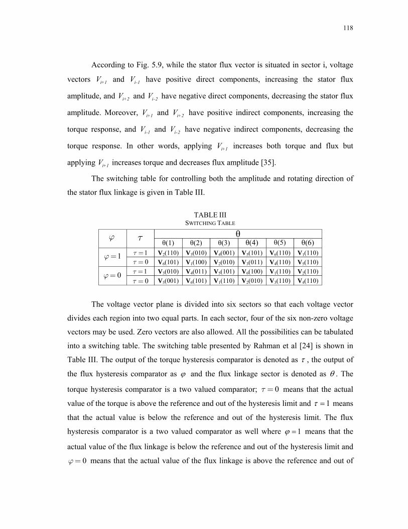
118
According to Fig. 5.9, while the stator flux vector is situated in sector i, voltage
vectors and V have positive direct components, increasing the stator flux
amplitude, and V and V have negative direct components, decreasing the stator flux
amplitude. Moreover, V and V have positive indirect components, increasing the
torque response, and V and V have negative indirect components, decreasing the
torque response. In other words, applying V increases both torque and flux but
applying V increases torque and decreases flux amplitude [35].
i+1V i-1
i+2 i-2
i+1 i+2
i-1 i-2
i+1
i+1
The switching table for controlling both the amplitude and rotating direction of
the stator flux linkage is given in Table III.
TABLE III
SWITCHING TABLE
V2(110) V3(010) V4(001) V5(101) V6(110) V1(110)V6(101) V1(100) V2(010) V3(011) V4(110) V5(110)V3(010) V4(011) V5(101) V6(100) V1(110) V2(110)V5(001) V6(101) V1(110) V2(010) V3(110) V4(110)
θθ(1) θ(2) θ(3) θ(4) θ(5) θ(6)
ϕ τ
1ϕ=
0ϕ=
1τ =0τ =1τ =0τ =
The voltage vector plane is divided into six sectors so that each voltage vector
divides each region into two equal parts. In each sector, four of the six non-zero voltage
vectors may be used. Zero vectors are also allowed. All the possibilities can be tabulated
into a switching table. The switching table presented by Rahman et al [24] is shown in
Table III. The output of the torque hysteresis comparator is denoted as τ , the output of
the flux hysteresis comparator as ϕ and the flux linkage sector is denoted as θ . The
torque hysteresis comparator is a two valued comparator; means that the actual
value of the torque is above the reference and out of the hysteresis limit and
0τ =
=1τ means
that the actual value is below the reference and out of the hysteresis limit. The flux
hysteresis comparator is a two valued comparator as well where 1ϕ =
0ϕ=
means that the
actual value of the flux linkage is below the reference and out of the hysteresis limit and
means that the actual value of the flux linkage is above the reference and out of

119
the hysteresis limit. Rahman et al [24] have suggested that no zero vectors should be
used with a PMSM. Instead, a non zero vector which decreases the absolute value of the
torque is used. Their argument was that the application of a zero vector would make the
change in torque subject to the rotor mechanical time constant which may be rather long
compared to the electrical time constants of the system. This results in a slow change of
the torque. This reasoning does not make sense, since in the original switching table the
zero vectors are used when the torque is inside the torque hysteresis (i.e. when the torque
is wanted to be kept as constant as possible). This indicates that the zero vector must be
used. If the torque ripple needs to be kept as small as with the original switching table, a
higher switching frequency must be used if the suggestion of [24] is obeyed [6].
We define ϕ and to be the outputs of the hysteresis controllers for flux and
torque, respectively, and as the sector numbers to be used in defining the
stator flux linkage positions. In Table III, if , then the actual flux linkage is smaller
than the reference value. On the other hand, if , then the actual flux linkage is
greater than the reference value. The same is true for the torque.
τ
(1) (6)θ θ−
1=ϕ
0=ϕ

120
5.3. Control Strategy of DTC of PMSM
+-
+- 2θ
1θ
6θ
3θ
4θ
5θ
30
Voltage Source Inverter (VSI)
( )32em D D Q QΤ P λ i λ i= −
( )
( )0
0
D D s D D
Q Q s Q Q
V R i dt
V R i dt
λ λ
λ λ
= − +
= − +
∫∫
2 2s D Qλ λλ = +
arctan Qs
D
λθ
λ=
CurrentSensors
PMSM
Voltage VectorSelection Table
HysteresisControllers
A
B
C
1 ( 2 )3
D a
Q a b
i i
i i i
=
= +1 ( 2 )3
D a
Q a b
i i
i i i
=
= +,D QV V
Dc-link voltage
sλ
emT
emT ∗
sλ∗
sθ
Initial rotorposition
Stator flux and torque estimator
iV
1
0
1
0
0Dλ 0Qλ,
Fig. 5.10. Basic block diagram of DTC of PMSM.
Fig. 5.10 illustrates the schematic of the basic DTC controller for PMSM drives.
The command stator flux, *sλ , and torque, , magnitudes are compared with their
respective estimated values. The errors are then processed through the two hysteresis
comparators, one for flux and one for torque which operate independently of each other.
The flux and torque controller are two-level comparators. The digital outputs of the flux
controller have following logic:
*emT
1λd = for *s s Hλλ λ< − (5.17)
0λd = for *s s Hλλ λ< + (5.18)
where is the total hysteresis-band width of the flux comparator, and is the
digital output of the flux comparator.
λ2H λd
By applying the appropriate voltage vectors the actual flux vector, sλ , is
constrained within the hysteresis band and it tracks the command flux, *sλ , in a zigzag
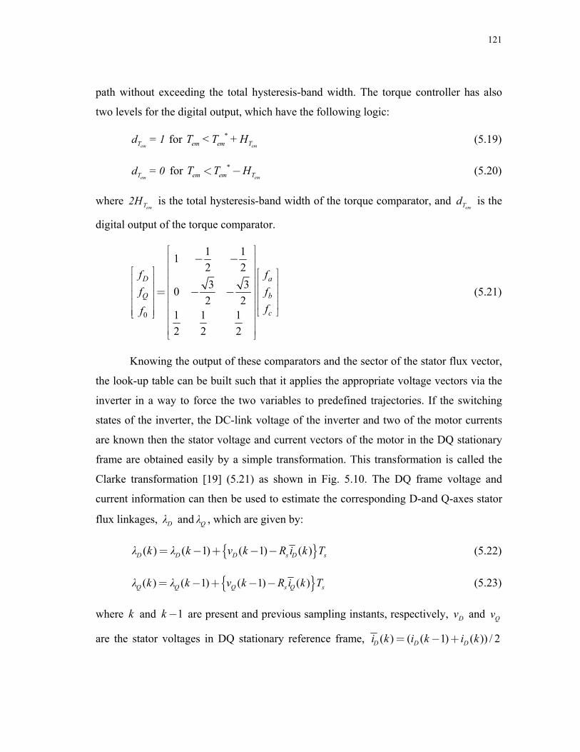
121
path without exceeding the total hysteresis-band width. The torque controller has also
two levels for the digital output, which have the following logic:
emTd = 1 for (5.19) em
*em em TT <T + H
emTd = 0 for (5.20) *emem em TT T H< −
where is the total hysteresis-band width of the torque comparator, and is the
digital output of the torque comparator.
emT2HemTd
0
1 112 23 30
2 21 1 12 2 2
D a
Q
c
b
f ff f
ff
⎡ ⎤⎢ ⎥− −⎢ ⎥⎡ ⎤ ⎡ ⎤⎢ ⎥⎢ ⎥ ⎢ ⎥⎢ ⎥⎢ ⎥ ⎢ ⎥⎢= − −⎢ ⎥ ⎥
⎢ ⎥⎢⎢ ⎥ ⎥⎢ ⎥⎢ ⎥⎢ ⎥ ⎣ ⎦⎣ ⎦ ⎢ ⎥
⎢ ⎥⎢ ⎥⎣ ⎦
(5.21)
Knowing the output of these comparators and the sector of the stator flux vector,
the look-up table can be built such that it applies the appropriate voltage vectors via the
inverter in a way to force the two variables to predefined trajectories. If the switching
states of the inverter, the DC-link voltage of the inverter and two of the motor currents
are known then the stator voltage and current vectors of the motor in the DQ stationary
frame are obtained easily by a simple transformation. This transformation is called the
Clarke transformation [19] (5.21) as shown in Fig. 5.10. The DQ frame voltage and
current information can then be used to estimate the corresponding D-and Q-axes stator
flux linkages, Dλ and Qλ , which are given by:
( ) ( 1) ( 1) ( )D D D s Dλ k λ k v k R i k= − + − − sT (5.22)
( ) ( 1) ( 1) ( )Q Q Q s Q sλ k λ k v k R i k= − + − − T (5.23)
where and are present and previous sampling instants, respectively, k 1k− Dv and
are the stator voltages in DQ stationary reference frame,
Qv
( ) ( ( 1) ( )) / 2D D Di k i k i k= − +

122
and ( ) ( ( 1) ( )) / 2Q Q Qi k i k i k= − + are the average values of stator currents, Di and ,
derived from the present, , and previous, , sampling interval values of
the stator currents,
Qi
( )DQi k ( 1DQi k − )
sR is the stator resistance, and sT is the sampling time. The stator
flux linkage vector can be written as:
2 2 1 ( )( ) ( ) ( ) tan
( )Q
D QD
λ kk λ k λ k
λ k−⎛ ⎞⎟⎜ ⎟= + ∠ ⎜ ⎟⎜ ⎟⎜⎝ ⎠
sλ (5.24)
where 2( ) ( )D Q2λ k λ k+ is the magnitude of the stator flux linkage vector and
1 ( )tan
( )Q
D
λ kλ k
−⎛ ⎞⎟⎜ ⎟⎜ ⎟⎜ ⎟⎜⎝ ⎠
is the angle of stator flux linkage vector with respect to the stationary
D-axis in DQ frame (or a-axis in abc frame). The developed stationary DQ reference
frame electromagnetic torque in terms of the DQ frame stator flux linkages and currents
is given by
3( ) ( ) ( ) ( ) ( )2em Q D D QΤ k P λ k i k λ k i k= −
)
(5.25)
where is the number of pole pairs. P
As it can be seen form (5.22) and (5.23) the stator resistance is the only machine
parameter to be known in the flux, and consequently torque, estimation. Even though the
stator is the direct parameter seen in (5.22) and (5.23), there is an indirect (hidden) motor
parameter for DTC of PMSM drives. This parameter is the rotor flux magnitude which
constructs the initial values of the D- and Q-axes stator fluxes. If the rotor flux vector,
, is assumed to be aligned with the D-axis of the stationary reference frame, then
equals the rotor flux amplitude
rλ
( 1Dλ k− r2λ . If the rotor magnetic flux, , resides on
the D-axis (the rotor magnetic flux can be intentionally brought to the known position by
applying the appropriate voltage vector for a certain amount of time), then the initial
value of the Q-axis flux, , is considered to be zero, therefore there will not be
any initial starting problem for the motor. On the other hand, if the rotor is in a position
rλ
( 1Qλ k − )

123
other than the zero reference degree then both the and values should
be known to start the motor properly in the correct direction without oscillation.
Moreover, if the initial values of the DQ frame integrators are not estimated correctly
then those incorrect initial flux values will be seen as DC components in the integration
calculations of the DQ frame fluxes. This will cause the stator flux linkage space vector
to drift away from the origin centered circular path and if they are not corrected quickly
while motor is running then instability in the system will result quickly.
( 1)Dλ k− ( 1Qλ k − )

124
CHAPTER VI
PROPOSED DIRECT TORQUE CONTROL (DTC) OPERATION OF PMSM
DRIVE
6.1. Introduction and Principles of the Proposed DTC Drive
In conventional DTC drives, there are some drawbacks, such as the DC drifts in
the voltage and current measurements, wrong DQ-frame initial flux linkages being used
or having resistance term exists in the estimation algorithm of the DQ stationary
reference frame flux linkages [36]. These disadvantages of the basic DTC scheme are
claimed to be eliminated by the proposed DTC technique.
Unlike the conventional DTC scheme which has a voltage model [24], the
proposed method is based on the current model which is considered in the rotor
coordinate system (rotor reference frame). By using the current model, the stator
quantities need to be transferred to the rotor reference frame quantities (this is ensured
by the position information). In this thesis, position information is provided by three
cheap hall-effect sensors (1$<) instead of bulky and expensive encoders or resolvers.
One hall-effect sensor is mounted on the stator starting from the boundary of Sector 1
and 2, and the remaining two hall-effect sensors are placed 120 electrical degrees apart
from each other in the counter-clockwise direction as shown in Fig. 6.1. The sector
change of the stator flux linkage space vector on the trajectory can be easily determined
by the help of the six hall-effect sensor signals that accompany one complete electrical
cycle.
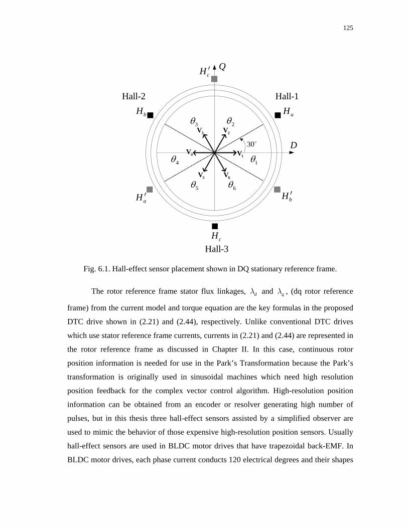
125
D
Q
2θ
1θ
6θ
3θ
4θ
5θ
2V3V
4V
5V 6V
1V30
aHbH
cH
bH ′aH ′
cH ′
Hall-1Hall-2
Hall-3
Fig. 6.1. Hall-effect sensor placement shown in DQ stationary reference frame.
The rotor reference frame stator flux linkages, and , (dq rotor reference
frame) from the current model and torque equation are the key formulas in the proposed
DTC drive shown in (2.21) and (2.44), respectively. Unlike conventional DTC drives
which use stator reference frame currents, currents in (2.21) and (2.44) are represented in
the rotor reference frame as discussed in Chapter II. In this case, continuous rotor
position information is needed for use in the Park’s Transformation because the Park’s
transformation is originally used in sinusoidal machines which need high resolution
position feedback for the complex vector control algorithm. High-resolution position
information can be obtained from an encoder or resolver generating high number of
pulses, but in this thesis three hall-effect sensors assisted by a simplified observer are
used to mimic the behavior of those expensive high-resolution position sensors. Usually
hall-effect sensors are used in BLDC motor drives that have trapezoidal back-EMF. In
BLDC motor drives, each phase current conducts 120 electrical degrees and their shapes
dλ qλ

126
are like square waveforms and their power devices are switched every 60 electrical
degrees to commutate the phase currents. The position sensor, therefore, has a resolution
of only 60 electrical degrees, thus an inexpensive low-resolution position sensor, such as
a hall-effect sensor, is suitable. On the other hand, in sinusoidal machines like PMSMs,
high-performance current vector control cannot be achieved and the operating
performance is inferior to the drive system which has low-resolution feedback position
information. The detailed explanation of position and speed sensing used in the proposed
DTC scheme by a simple observer assisted with three low-cost hall-effect sensors will be
discussed in the next section.
Once the position is estimated by the three hall-effect sensors, the Park’s
Transformation is applied to the three phase abc frame currents that are measured to get
the dq rotor reference frame currents. After that, the obtained dq rotor reference frame
currents are placed in (2.21) to estimate the stator dq axes flux linkages. With this
information, the stator flux linkage amplitude can be derived as:
2 2s d qλ λ λ= + Equation Section 6(6.1)
The stator flux linkage amplitude calculated from rotor reference frame
quantities is exactly the same as the one found by using the stator reference frame fluxes
Dλ and as shown in Fig. 6.2. Qλ

127
reω
sω
δ
sλ
rλ
Q
Dreθsθ
d dL i
q qL i
Dλ
Qλq
d
Fig. 6.2. Representation of the rotor and stator flux linkages both in the synchronous dq
and stationary DQ-planes.
Although the stator flux linkage amplitude calculation in both the stator and rotor
reference frames generates the same result, the exact position of the stator flux vector in
the DQ frame cannot be applied to the rotor reference frame flux components by just
using (5.27). The angle between the rotor reference frame q-axis flux and d-axis flux,
which is a constant value due to the DC values of the synchronous frame currents equals
to the load angle,δ , and the stator flux vector angle, sθ , with respect to the D-axis, is
given by:
arctan qs r r
d
λθ θ θ
λ
⎛ ⎞⎟⎜ ⎟= + = +⎜ ⎟⎜ ⎟⎜⎝ ⎠δ (6.2)
With the proposed method, the initial flux errors which cause drift in the basic
DTC scheme will not be added to the next calculations (integration). The only problem
in flux calculations might happen at high current and high temperature. The rotor
reference frame stator flux linkages possess d- and q-axes inductances along with a rotor
magnetic flux linkage amplitude which is affected by an increase in temperature. Under
magnetic saturation the q-axis inductance of an IPMSM varies and the d-axis inductance
is affected by the armature reaction therefore the saturation model for various load

128
conditions should be developed such that inductance should be expressed taking into
account magnetic saturation. Also, when the load is increased the amplitude of the rotor
magnetic flux linkage is increased (due to temperature rise) therefore it is necessary to
consider the change in the synchronous inductance ( s d qL L L= = in surface-mounted
PMSMs) because it is greatly affected due to magnetic saturation. Magnetic saturation
and temperature effects are not included in the proposed system, but it should be
considered and compensated for if there is high current and the operating points of the
current reside in the saturation region of the motor.
Basic DTC is based on a voltage model which is plagued by the stator resistance
error and the integration drift at low frequencies. On the other hand, the current model is
affected by parameter detuning (due to magnetic saturation) and also by the position
error, but it works pretty well from zero speed if a high-resolution position sensor such
as an encoder is used. In the literature, a combination of the voltage and current model is
proposed with a PI compensator such that the current model is predominant at low
speeds while the voltage model takes over at high speeds. Applications of this combined
method can be very costly due to the additional sensor (position). To make the overall
system cheaper, the current model is suggested instead of the voltage model therefore
only a very cheap position sensor is needed (hall-effect sensor). A complete block
diagram of the proposed DTC scheme is given in Fig. 6.3. Because the motor used in
this thesis is a high torque motor and in washing machine applications there is a certain
limit for the capacity of the load (approximately known load torque) in the drum such
that currents cannot bring the motor into the saturation region easily, thus inductance
compensation can be ignored. In certain applications where very high currents bring the
motor to the saturation region and temperature increases inside the motor are evident, the
inductance and amplitude of the rotor flux linkage should be compensated.
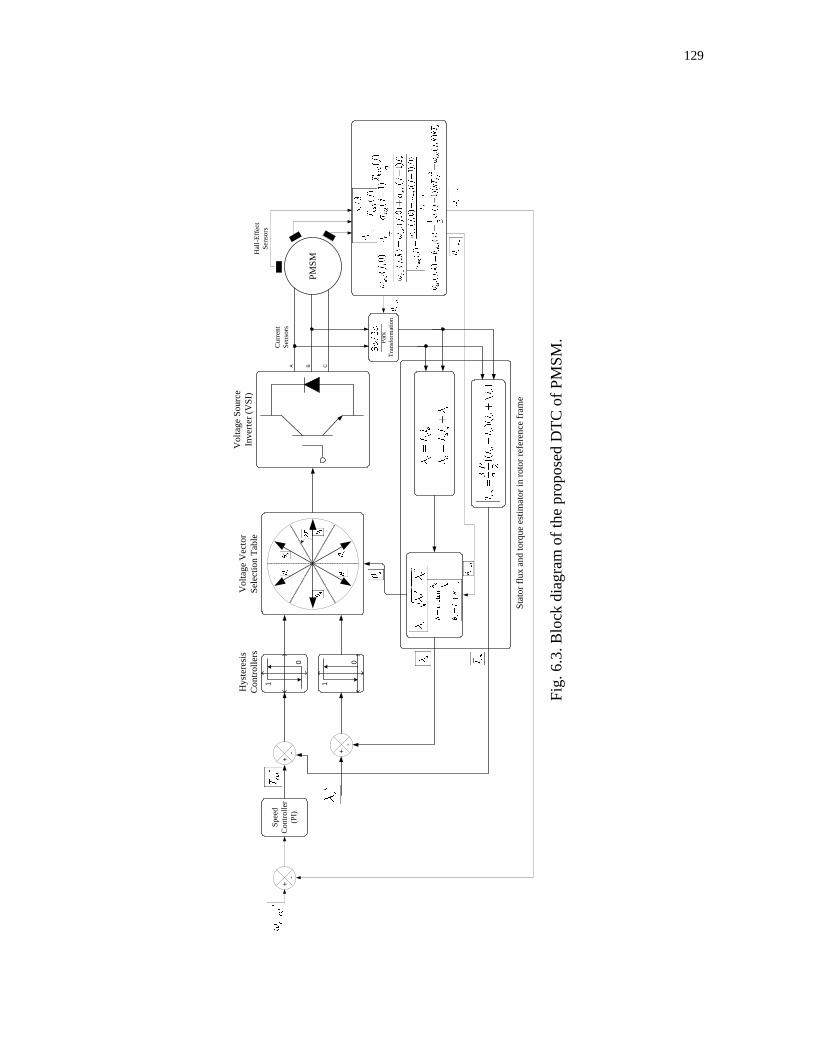
129
+-
+-
Vol
tage
Sou
rce
Inve
rter (
VSI
)
Cur
rent
Sens
ors
PMSM
Vol
tage
Vec
tor
Sele
ctio
n Ta
ble
Hys
tere
sis
Con
trolle
rs
A B C
Park
Tran
sfor
mat
ion
Stat
or fl
ux a
nd to
rque
est
imat
or in
roto
r ref
eren
ce fr
ame
Spee
dC
ontro
ller
(PI)
+-
Hal
l-Eff
ect
Sens
ors
1
0
1
0
Fig.
6.3
. Blo
ck d
iagr
am o
f the
pro
pose
d D
TC o
f PM
SM.

130
6.2. Position and Speed Estimation Method with Low-Resolution Position Sensor
In permanent magnet synchronous motors (PMSMs) and for every other
sinusoidal current controlled AC drive systems, in order to produce the sinusoidal
current commands and control the current phase accurately, high resolution position
information is essential. A high resolution position sensor such as an optical encoder
with large pulses per revolution or a resolver is therefore usually used.
Since the current model is used for the proposed DTC of a PMSM drive,
continuous rotor position information should be obtained. In this thesis, a low resolution
position sensor which has an accuracy of only 60 electrical degrees is used instead of a
high resolution sensor. Such low-resolution position feedback can be achieved by the
processed signals from three cost-effective hall-effect sensors as shown in Fig. 6.1. One
electrical cycle is divided into six intervals (representing the six sectors for the DTC
scheme) of 60 electrical degrees by the processed signals , , and . In this case,
the absolute position with an accuracy of 30 electrical degrees (mid point of two
consecutive hall-effect signals are chosen as a reference point) can be obtained, and as a
result reverse rotation at starting never occurs. The hall-effect sensor has advantages
such as smaller size and lower cost compared to an optical encoder or resolver.
However, since the position updates occur at every 60 electrical degree interval, the
necessary continuous position information for PMSM drives cannot be achieved by
using just three hall-effect sensors like in BLDC drives. Knowing this, vector
transformations (Park’s and inverse Park’s Transformations) and sinusoidal current
drives cannot be achieved by using low-resolution position sensing. The main goal of
this thesis is to estimate higher resolution position information from the rough position
information obtained from the three hall-effect sensors. The method of obtaining the
high-resolution position information from the three hall-effect sensor signals is
explained using Fig. 6.4 as follows:
aH bH cH
±
In Fig. 6.4, the actual positions, ( )real jθ , corresponding to , , 120 , 180 ,
, and 30 are obtained from the three hall-effect sensors at every 60 electrical
degrees. The index pointer of the corresponding component is defined as
0 60
240 0
j and 1j− is
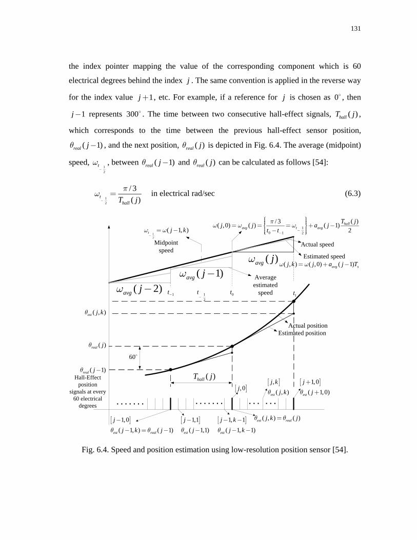
131
the index pointer mapping the value of the corresponding component which is 60
electrical degrees behind the index j . The same convention is applied in the reverse way
for the index value 1j + , etc. For example, if a reference for j is chosen as , then 0
1j− represents . The time between two consecutive hall-effect signals, ,
which corresponds to the time between the previous hall-effect sensor position,
, and the next position,
300 ( )hallT j
( 1real jθ − ) ( )real jθ is depicted in Fig. 6.4. The average (midpoint)
speed, 1 2
tω−
, between and ( 1)real jθ − ( )real jθ can be calculated as follows [54]:
1 2
/ 3( )t
hallT jπ
ω−
= in electrical rad/sec (6.3)
. . . . . . . . . . . . . . . . .
( 2)avg j−ω( 1)avg j−ω
( )avg jω
1 0 1 2
( )/ 3( ,0) ( ) ( 1)2
hallavg t avg
T jj j a jt tπ
ω ω ω−
−
⎧ ⎫⎪ ⎪⎪ ⎪= = = + −⎨ ⎬⎪ ⎪−⎪ ⎪⎩ ⎭12
( 1, )t j kω ω−
= −
Midpoint speed
1t− 12
t−
0t
( , ) ( ,0) ( 1)avg sj k j a j Tω ω= + −
Estimated positionActual position
( , )est j kθ
( )real jθ
( 1)real jθ −
60
( )hallT j
1t
[ ]1,0( 1, ) ( 1)est real
jj k jθ θ
−
− = −
[ ]1,1( 1,1)est
jjθ
−
−
[ ]1, 1( 1, 1)est
j kj kθ
− −
− −
[ ], 0j[ ],
( , )est
j kj kθ
( , ) ( )est realj k jθ θ=
[ ]1,0( 1,0)est
jjθ
+
+
. . .
Hall-Effect position
signals at every60 electrical
degrees
Average estimated
speed
Actual speed
Estimated speed
Fig. 6.4. Speed and position estimation using low-resolution position sensor [54].

132
1 2
1 2 / 2
t
mt P
ωω
−
−
= in mechanical rad/sec (6.4)
where is the pole numbers of the motor. P
At each 60 electrical degree interval time the speed of the rotor including the
average acceleration or deceleration rate can be defined as:
1 2
( )( ,0) ( 1)2
hallest t avg
T jj a jω ω−
= + − (6.5)
To resemble the high-resolution position sensing phenomenon, the rotor position
and speed corresponding to the well-known Newton’s motion law between two
consecutive hall-effect signals can be estimated as follows:
( , ) ( ,0) ( 1)est est avg sj k j a j Tω ω= + − (6.6)
where sT is the sampling time of the overall system.
At every 60 electrical degrees (hall-effect sensor signal observed) the average
rotor acceleration or deceleration rate (… , , …) is calculated as: ( 1)avga j− ( )avga j
1
( ,0) (( 1),0)( ) est estavg
j j
j ja jt t
ω ω
−
− −=
− electrical rad/s2 (6.7)
where is the time at (( and is the time at 1jt − 1),0)j− jt ( ,0)j as shown in Fig. 6.4. The
present estimated position between two consecutive hall-effect sensor signals, ( , )est j kθ ,
when the acceleration or deceleration is ignored can be expressed as:
( , ) ( ) ( , )est real Pj k jθ θ θ= + j k
s
(6.8)
where denotes the incremental position added to the real position
which is obtained from the hall-effect sensor. Replacing that into (6.8), we obtain:
( , ) ( )P avgj k j kTθ ω=
( , ) ( ) ( )est real avg sj k j j kTθ θ ω= + (6.9)

133
Using angular velocity, ( , )est j kω , the present estimated position, ( , )est j kθ , is
calculated by adding the real position, ( )real jθ , obtained from the hall-effect sensors to
the estimated incremental position, , and also it is the angle rotated from the actual
position to the present that is represented by:
( )P kθ
( )21( , ) ( ) ( 1) ( , )2est real avg s est sj k j a j kT j k kTθ θ ω= + − + (6.10)
The real position, ( )real jθ , can be expressed when as: 0k =
( ) ( ,0)real estj jθ θ= (6.11)
where in the above equations is the index pointer representing the incremental value
of the sampling time,
k
sT , starting at 0 incrementing by one.
Basically, in the above method position is collected from the hall-effect sensors
and the average acceleration or deceleration rate of the rotor is calculated at every 60
electrical degrees interval. The estimated rotor position and the speed values between
those intervals are obtained by using Newton’s motion law equations given above.
Fig. 6.5 depicts the acceleration and speed estimations in each sector and at the sector
boundaries of the proposed DTC scheme, respectively. Because the acceleration or
deceleration of the motor is included in the above position and speed estimation
equations, the hesitation problems associated with step and ramp speed references under
initial load condition are sufficiently improved.
Even though the rotor position is calculated from (6.10), it needs to be clarified
that if the estimated rotor position is still within the assumed section. For example, if the
rotor is assumed to be in the Sector 1, the condition that should be
satisfied. The estimated rotor position is corrected when the limits exceeded for Sector 1.
The correction logic that is used in the Sector 1 is given below [55]:
330 30rθ≤ ≤
If , then ; 330rθ < 330rθ =
If , then . 30rθ > 30rθ =
There are four major advantages associated with the proposed algorithm [55]:

134
• No parameter sensitivity problem because no machine or drive
parameters are used in the rotor position estimation.
• No error accumulation problem as the rotor position is reset at every 60
electrical degrees.
• No starting problem because the hall-effect sensors provides enough
information for correct starting. There will be no wrong direction start.
• Low cost contrary to expensive high precision position sensors such as
optical encoders and resolvers and high reliability as compared to
encoders and resolvers.
• Simple algorithm can be easily implemented by a microprocessor or DSP.
As the rotor position corrects itself at every section transition, the position
estimation error is very reasonable at high speeds and even during dynamic transients.
The estimation algorithm proposed in this thesis guarantees the estimated
position with high accuracy at low speeds.
D
Q
30
aHbH
cH
bH ′aH ′
cH ′
Hall-1Hall-2
Hall-3
1a
2a3a
4a
5a 6a
1 1, tω
2 2, tω
3 3, tω
4 4, tω
5 5, tω
6 6, tω
7 7, tω
Fig. 6.5. Representation of acceleration and speed at the sectors and at the hall-effect
sensors, respectively.

135
CHAPTER VII
AGITATION PERIOD SPEED CONTROL OF VERTICAL-AXIS
LAUNDRY MACHINE
7.1. Modern Washing Machines: Top Loaded (Vertical-axis) vs. Front Loaded
(Horizontal-axis) Washing Machine
Contemporary washing machines are available in two main configurations:
“top-loading” and “front-loading”. The “top-loading” design, the most popular in the
US, Australia, and some parts of Europe, has the clothes placed in a vertically-mounted
cylinder with a propeller-like agitator in the center of the bottom of the cylinder. The
cloths are loaded at the top of the machine, which is covered with a hinged door. The
“front-loading” design, the most popular in Europe (especially in UK), instead mounts
the cylinder horizontally, that allows loading through a glass door at the front of
machine. The cylinder is called the drum.
Tests comparing front-loading and top-loading machines have shown that, in
general, front-loaders wash cloths more thoroughly, cause less wear, and use less water
and energy than top-loaders. As a result of using less water, they require less detergent.
They also allow a dryer to be mounted directly above the washer, which is impossible
with a top-loader. On the other hand, top loaders complete washing much faster, tend to
cost less for the same capacity machine, and allow clothes to be removed at intermediate
stages of the cycle (for instance, if some clothes within a wash are not to be spun).

136
7.2. Introduction to Speed Control of a BLDC Spindle Motor (48 Pole/36 slot) in
The Agitation Cycle of a Washing Machine
In a vertical-axis washing machine, agitation is supplied by the back-and-forth
rotation of the cylinder (drum) and by gravity. The items are lifted up by paddles in the
drum, and they are then dropped down to the bottom of the drum. This motion forces the
water and detergent solution through the fabric. Although more infrequent, there is also a
variant of the horizontal axis design that is loaded from the top, through a flop in the
circumference of the drum. These machines usually have a shorter cylinder and are
therefore smaller [56].
In the agitation part of a laundry washing cycle, the controller controls the power
supplied to the motor using Pulse Width Modulation (PWM) in order to maintain motor
speed in accordance with a predetermined speed profile. The agitation speed profile can
be categorized into three sections [56]:
(i) Ramp up from standstill to a desired plateau speed (steady-state speed), the
so called “acceleration” or “ramp” region.
(ii) Maintaining the plateau speed for a predetermined period of time. This
section is called the “plateau” region.
(iii) Removing the motor power by turning off the lower switches of three-phase
inverter and coasting the motor towards zero speed. The end of plateau
section is the start of the coast section. Once the speed of the motor drops to
the predetermined reversal speed, which is usually defined as half of the
reference plateau speed, motor will be reversed. If it is necessary, after
reaching the reversal speed, the motor will be turned in reverse direction
when the motor speed drops to zero. Consequently, the time between the end
of plateau section and reversal speed is called the “coast” time and the time
between the reversal speed and the zero speed in one stroke is called the
“pause” time. Altogether the coast and pause time establish the “coast/pause”
region of a stroke.

137
The combination of (i), (ii), and (iii) is the stroke time of the washing machine in
the agitation cycle. At the end of each stroke, the motor direction is reversed. In each
agitation stroke, the stroke time is controlled by adjusting the “coast” (pause time is
constant) phase of each stroke in order to maintain consistent washing performance.
Before starting the agitation washing cycle, all of the above phases (times) determined
by the controller depending on the load condition are chosen using the information given
on the washing machine panel by the customer. Only the ramp, plateau phases and pause
times stay constant in every stroke. The “coast” phase is initiated, however, (after a
predetermined period elapsed in the “plateau” phase) by starting a timer and allowing the
motor to coast until the motor velocity (speed) drops to a predetermined reversal speed
at which point the motor is reversed to begin the next agitation stroke. Several
experiments have proven that the reversal speed should be chosen to be equal to the half
of the plateau speed and can be adjusted depending on the load conditions (bunching,
etc.). Reversal speed will be changed in accordance with the difference between the
timer value when the velocity reaches the reversal speed and the predetermined timer
value representing the total coast time. If the timer value is greater than the desired value
or range of values then the predetermined value of the reversal speed will be increased.
Alternatively, if the timer value is less than the desired value or range of value the
reversal speed will be decreased. Eventually, the period of the coast phase of the next
stroke should be closer to the desired period. The “coast/pause” phase is not going to be
the main focus in this thesis work, instead the “ramp” and “plateau” phases will be the
main subjects to be discussed. A simple flowchart of the agitation speed control is
depicted in Fig. 7.1.

138
Initialize( Set Plateau Speed, Ramp Time, Plateau
Time, Pause Time)
Ramping
Steady-state (Plateau region)
Coasting/Pause
Reversing
Fig. 7.1. Simple flowchart of the commercial agitation speed control [57].
7.3. Agitate Washer Controller Model in SIMPLORER®
A complete agitation washer controller is built in SIMPLORER®. Unlike a
real-time microcontroller that uses interrupts and counters, the simulation will use time
based logic for simplicity. Details are as follows:
As explained before, the agitator speed controller has ramp, plateau, coast and/or
pause time sections in the reference speed profile which is shown in Fig. 7.2. Basically,
the controller has four inputs. Those are: Plateau Speed (PS), Ramp Time (RT), Plateau
Time (PT), and Pause Time (PaT). Coast Time (CT) is an input usually maintained at a

139
certain predefined time by the controller. In this thesis, the coast and pause sections are
not modeled fully. They were discussed briefly in the previous section. Characteristics of
each section will be explained. One positive complete cycle (stroke) is shown in the
graph below. The negative cycle which has the same shape, but in reverse direction, is
not shown here, the reverse rotation starts when the cost/pause section is over.
t(ms)
Plateau Speed
Ramp Time Plateau Time
Pause Time/Coast Timewref* (rpm)
1 2 3
Fig. 7.2. Reference speed profile for the agitation speed control in a washing machine.
The operation of the agitation control in a laundry washing machine algorithm
used in commercial washing machines is discussed below. A flowchart is provided
detailing the operation of the simple agitation washing controller which is implemented
in the simulation platform, SIMPLORER®.

140
Accelerate motor to plateau speed
START
Overshoot compensation,attain and maintain plateau speed
Plateau periodcompleted?
Remove motor powerStart timer. TIME=0
Motor speed = reversalspeed?
Stop timerTimer = elapsed coast time
Elapsed coast time > preferred coast
period (range)?
Elapsed coast time < preferred coast
period (range)?
Increment reversal speed Decrement reversal speed
Agitation cyclecompleted
Reversal motor direction
Stop agitating
Fig.7.3. Detailed flowchart of the simple agitation speed control of a washing machine
[58].

141
Fig. 7.3 presents the instructions required to carry out the agitation phase of a
washing cycle with a detail flowchart. Descriptions of that flowchart are as follows:
When the washing machine has completed a fib phase and the laundry load is
floating (or submerged) in a suitable mixture of water and detergent, the motor is
accelerated (ramped up) incrementally by increasing the PWM duty cycle starting at a
minimum value up to plateau speed. More details about ramping up the motor to the
desired plateau speed will be discussed later.
Due to the inertia of the drum and laundry load speed overshoot can occur,
therefore an overshoot compensation algorithm is developed to bring the exceeded motor
speed down to the desired plateau speed as quickly as possible. When the plateau speed
is achieved after applying the overshoot compensation (if it is necessary) then the
desired plateau speed is maintained till the predetermined “plateau” region is completed
(by checking the motor controller timer). At the end of the plateau region the motor
power is removed by turning off the lower side of the inverter switches. At the same
time the motor timer is started from zero to determine the length of the coast section.
While the coasting condition is continuing the reversal speed may be reached (which is
assumed to be half of the plateau speed). As time elapses during this phase, the total
coast region length is determined for use in the adaptation mechanism of the next
strokes. The elapsed coast time is then compared with the predetermined coast time. If
the measured coast time is greater than the desired coast period (or range of periods)
then the controller increments the reversal speed to be used in the next stroke. If the
measured coast time is less than the desired coast period the controller decrements the
reversal speed for the next stroke. One stroke late adaptation algorithm is therefore
established by controlling the coast time because if the reversal speed for the next cycle
is higher than what was defined previously then the coast time will be shorter and vice
versa, eventually causing a change in the length of the stroke time. If the pause time is
defined as zero then the agitation reverses the motor and the same method is applied
until the agitation phase of the washing cycle is completed. Agitation is then stopped and
the control executes the next washing cycle. If, however the agitation phase is not yet

142
complete, then the motor direction is reversed and power is reapplied to the motor
windings where the above described process is repeated until the end of the agitation
phase [56].
1) Ramp-up Section:
As it is known in DC motor control, to increase the rotational speed of the motor
the PWM duty cycle of the inverter outputs should be increased. To reduce the speed of
the motor the duty cycle should be decreased, as a result it can be stated that the change
in the duty cycle is proportional to the change in speed. The duty cycle of the PWM
signal which is applied to the motor terminals by a VSI inverter is determined by the
following equation:
max
_ (%) 100 / currentPWMduty cyclePWM
⎛ ⎞⎟⎜ ⎟= ⎜ ⎟⎜ ⎟⎜⎝ ⎠ (7.1)
The ratio above determines the on time of the one PWM period (PWM frequency
can be any value not less than 2 kHz). If becomes equal to the full
DC-link voltage will be applied to the motor terminals and maximum speed will be
achieved. In starting, is chosen as small as possible to handle the light load.
is the key component to decide the resolution of the speed increment. If it is
higher and the incremental rate of is small then a higher speed increment
resolution is achieved, but if it is small and the incremental rate is bigger
then a lower speed increment resolution is provided.
currentPWM maxPWM
currentPWM
maxPWM
currentPWM
currentPWM
In ramping, the PWM rate is incremented till the end of ramp period. At that
moment the speed is measured by the help of three hall-effect sensors which provide
electrical signals indicative of the rotor position. These signals are then fed to the input
of a microcontroller via an interface circuit. According to the resultant speed feedback,
(along with the duty cycle) is adjusted up or down depending on whether the
measured speed is too low or too high.
currentPWM

143
As several tests show, regardless of how fast the agitation period is, it is possible
to have any ramp period from (e.g. 80 ms – 400 ms) for a better speed profile with less
overshoot under heavy laundry load conditions. The ramp time also depends on the wash
profile; if it is very gentle then soft agitation is desired therefore a longer ramp up time is
preferred and vice versa.
plateauV
PWM increments
currentPWM
PT
( )Time s
( )Speed RPM
Fig. 7.4. PWM increment during the ramp time [58].
currentPWM is incremented at every PT (sampling time of the in
ramping) as shown in Fig. 7.4 in a series of incremental steps, therefore the speed of the
motor gradually increases because the PWM increment occurs at every time interval
currentPWM
PT
as shown in Fig. 7.5.

144
plateauV
currentPWM
PT
( )Time s
( )Speed RPM
RampT
Fig. 7.5. Speed response during ramp up when PWM is incremented at every PT time
[58].
In Fig. 7.4 the angular speed is shown diagrammatically as increasing in discrete
steps. Each step corresponds to an increase in which also increases the duty
cycle of the PWM signal. The smaller
currentPWM
PT is the more is incremented
therefore more power is supplied to the motor. All the above descriptions given about
ramping up are summarized as follows: is started at a certain number which
can handle the light laundry load at starting and a certain increment step value is chosen
(e.g. 16) such that the step time,
currentPWM
PWMcurrent
PT , (also known as the sampling time) of
can be found if the ramp time is known by the following formula:
currentPWM
_P
Ramp TimeTSTEPS
= (7.2)
At every sampling time the value is incremented by a certain
predetermined amount until the speed reaches the desired plateau speed in the
predetermined ramp time. If the actual speed is less than what is necessary then ramp
currentPWM

145
adjustment is used starting from the very next stroke. The ramp adjustment algorithm is
a mandatory tool in agitation control. For example, the load on the motor can not always
be the same due to varying wash loads, and it is not possible to predetermine the number
of incremental steps in order to obtain the correct speed within the ramp time.
A small amount of power (i.e. a small duty cycle value) is enough to start
accelerating the motor to the desired plateau speed during the ramp time when there is a
very light load on the machine. With a heavy load more power (larger duty cycle value)
will be required. The amount of power that can be supplied to accelerate the motor to the
desired plateau speed in the predetermined ramp time is proportional to the rate of
increase of the incremental steps. The number of steps is initially preset to a minimum
setting so that no adjustment is needed for very light loads. Let’s say a machine has a
very light load and 6 incremental steps are necessary to accelerate the motor to a desired
plateau speed in a predetermined ramp time (e.g. 100 ms). On the other hand with a
heavy load 62 steps might be required to reach the same speed in same amount of time
(100 ms). The software therefore needs to adjust the number of steps to attain the desired
speed at a desired interval time. This is performed when the speed is first time monitored
at the end of the ramp time at every stroke. If the measured speed at the end of the ramp
period is found to be under the desired plateau speed then the number of steps is
incremented, thus the value of increases, and hence the torque of the motor
increases [58].
currentPWM
2) Plateau Section:
Ideally, in the plateau region, a constant speed is maintained for a desired
predetermined plateau time period. This is the case when there is no heavy load (too
much laundry load) on the motor, but at extremely heavy loads a normal agitate
controller cannot maintain the speed at the desired plateau speed due to torque
constraints on the motor. There is a need for overshoot control in the plateau region to
ensure the speed maintains an ideal profile at heavy loads, as shown in Fig. 7.6.

146
plateauV
( )Time s
12 plateauT 1
2 plateauT
plateauT
( )Speed RPM
Fig. 7.6. Ideal speed profile of the agitation speed control [58].
Under very heavy loads the actual profile digresses from the desired speed
profile as shown in Fig. 7.7. Several experiments show that the load condition of the
motor during the plateau region is not its heaviest until approximately half way through
the plateau region. If the load in the drum is increased, then the tail end of the plateau
region begins to diverge ¾ of the way through the plateau region, hence the best point to
measure the speed and determine when to add or subtract compensation is at the mid
point of the plateau region as illustrated in Fig. 7.7 [58].

147
plateauV
( )Time s
plateauT
tΔ
plateauVΔ
( )Speed RPM
Fig. 7.7. Typical practical speed response of the agitation speed control [58].
If the measuring point indicates a speed that is under the desired plateau speed
then on the next stroke cycle at the end of the ramp period the software will increase the
plateau speed by an error received from the compensation algorithm, Δ , for a
predetermined time, , as seen in Fig. 7.7. As the load increases, the compensation
should also increase. The first parameter that is increased is the overshoot time, .
This is increased until either the speed has reached a desired value at the measuring point
(mid point of the plateau region) or Δ is equal to the plateau time [58].
plateauV
tΔ
tΔ
t
If is equal to the plateau time and the speed at the measuring mid point is still
under the desired speed due to very heavy load, then the overshoot speed, , is
increased until a predetermined limit is reached or the speed at the measuring mid point
is acquired [58].
tΔ
plateauVΔ
If the maximum compensation limit has occurred but actual speed measured at
the mid point of the plateau region is still under the desired plateau speed due to heavy
load condition, however, then the ramp rate is increased by increasing the number of
steps, as explained above, in relation to the acceleration ramp control.

148
CHAPTER VIII
EXPERIMENTAL AND SIMULATION ANALYSIS
8.1. Open-Loop Simulation vs. Experimental Results
In this section of Chapter VIII, before going into the detailed discussion of the
simulation and experimental results of the commercialized agitation cycle speed control,
an open-loop steady-state and transient-state simulation and experimental results will be
given and those results discussed and compared. The experimental setup of the
open-loop control system is explained in detail. Important motor parameters such as
efficiency and power factor, are measured in both the simulation and experiment.
Open-loop analysis and suggested measurement methods of those motor parameters are
explained in detail.
8.1.1. Open-Loop Steady-State and Transient Analysis (Simulation)
Open-loop (V / f control) MATLAB/SIMULINK® simulations have been
conducted to verify and compare the performance of the simulated 48 pole PMSM with
the real model. All the open-loop steady-state and transient state simulations are carried
out using the default variable-step ode45 (Dormand-Prince) algorithm. The maximum
step size, relative tolerance and absolute tolerance are all set to 1e-3. Several parameters
such as power factor, efficiency, rms motor phase current, and load angle are simulated
at a 100 rpm (40 Hz) steady-state operating speed to compare with the experimental
results to verify how close the simulated motor model is to the real motor. A three-phase
AC voltage source is used to implement the open-loop V / f control in the simulation of
the PMSM.

149
The PMSM cannot be started at reasonable high constant frequencies, such as
40 Hz, which is used in our tests, so in the simulations the initial speed is selected as
40 Hz (100 rpm) instead of 0 Hz to overcome this problem. The V / f ratio is set to 2,
meaning an 80 Vrms sinewave signal with 40 Hz frequency will be generated. By
choosing V / f ~= 2, a good speed result (no pulsation) and better current shapes (close
to pure sinusoidal and less oscillation) are obtained, and the results of efficiency, power
factor, rms motor phase current (Phase A) and motor speed versus load torque are
displayed in Fig. 8.1 in comparison with the experiments. It is observed that the
simulation results are very close to the experiments, especially at low load torque values
since the parameter change effect is not considered in the simulations when the load
torque increases up to 10 N·m a discrepancy occurs at high temperature (rotor flux
linkage amplitude and resistance are affected by temperature change). If the saturation
level of the motor is reached and exceeded then the synchronous inductance value will
also alter.
A transient analysis is performed to observe the starting performance of the
simulated model in comparison with the experimental results; basically this test has been
done to verify the inertia and other torque effective components such as friction and
windage load etc. on the transient conditions. From Figs. 8.2 and 8.3, it can be seen that
the simulation speed response to the step input is faster than the experimental result.
Having a transient response in open-loop is quite challenging due to the lack of position
information to synchronize the rotor field with stator rotating field at start up. If the
transient is less than 0.4 second both responses converge and reach the steady-state
speed. To start the motor properly in both simulation and experimental transient tests,
the zero initial position is selected as the reference point. Any position can be chosen as
a reference, but since the input voltage is a sinewave, starting the motor from the zero
position generates less torque pulsation. In general, the zero reference position is the
position when the rotor flux is aligned with the Phase A axis. In practice, if the neutral
access is available then enough DC voltage is applied between Phase A and the neutral
point to enable the rotor to stay aligned with the Phase A axis. If the neutral is not

150
available then Phase B and C are short-circuited, so when DC voltage is applied between
Phase A and the short-circuited Phase B and C the same zero position alignment will be
achieved.
100 RPM (40 Hz) Open-Loop (V/f=2) Experimental vs. Simulation Results (80Vrms Sinewave Input,Ld=Lq=92.7274mH)
0
0.2
0.4
0.6
0.8
1
1.2
1.4
1.6
1.8
0 2 4 6 8 10 12
Torque (Nm)
Eff,
PF,Ia
0
30
60
90
120
150
Speed
Exp. Efficiency Exp. Ia (Amp) Exp. PF Sim Ia (rms) Sim. Eff Sim. PF Exp. Speed (RPM)
Fig. 8.1. Efficiency, power factor, motor current (Phase A), and motor speed versus
applied load torque (open-loop exp. and sim.) at 100 rpm with V / ~= 2. f

151
0-37.5 RPM Experimental and Simulation Dynamic Speed Responds (V/f=18/15)
0
5
10
15
20
25
30
35
40
45
50
0 0.1 0.2 0.3 0.4 0.5 0.6 0.7 0.8 0.9 1
Time (s)
Spee
d (R
PM)
Exp.Speed Sim.Speed
Fig. 8.2. Dynamic speed response of exp. and sim. when V / f = 18/15 (0-37.5 rpm).
0-37.5 RPM Experimental and Simulation Dynamic Speed Responds (V/f=1)
0
5
10
15
20
25
30
35
40
45
50
0 0.1 0.2 0.3 0.4 0.5 0.6 0.7 0.8 0.9 1
Time (s)
Spee
d (R
PM)
Exp.Speed Sim.Speed
Fig. 8.3. Dynamic speed response of exp. and sim. when V / f = 1 (0-37.5 rpm).

152
8.1.2. Open-Loop Steady-State and Transient Analysis (Experiment)
Experimental tests have been conducted on a 325 PM synchronous machine
(sinusoidal back-EMF) with 48 rotor poles. Even though the agitation control algorithm
generates squarewave currents to control the motor, in an open-loop test the sinewave
input voltages are used to get better performance on the measurements of the efficiency,
power factor, load torque, and rms phase current of the motor. Since the current is
rectangular in agitation control, but the back-EMF of the machine is sinusoidal, the
resultant torque (electromagnetic torque) is not smooth. Fig. 8.4 shows the
electromagnetic torque of a PMSM having a sinusoidal back-EMF when it is driven with
square-wave currents.
dcV
Time (s)
Torque (N.m.)
Fig. 8.4. Torque response of PMSM when it is supplied by quasi-square wave currents.
In the open-loop transient test, the rotor is locked with the zero position as
explained above and a three phase programmable AC voltage source is connected to the
motor terminals. The minimum frequency available from the power source, 12 Hz, is
chosen such that the V / f ratio will be around 1. With this V / f ratio the rms value of
the sinusoidal voltage becomes 12 Vrms. Additionally, a second test for transient
analysis is performed with V / f ~= 18/12. During this test, a dynamometer controller
(DSP600) is used so the speed response can be stored in the M-TEST 4.0® software and
saved as a Microsoft® Excel spreadsheet as shown in Figs. 8.2 and 8.3.
The open-loop efficiency calculation, explained in Chapter IV, which is done in
MATLAB/SIMULINK® shows an agreement with the actual measurement provided by
the Magtrol Power Analyzer Model 6530, as shown in Fig. 8.1. Measurements of real

153
power, power factor, efficiency, motor voltages and currents, etc. are obtained in the
M-TEST 4.0® software which communicates with the power analyzer through the GPIB
cable. Other necessary equipment for measuring the above parameters include a Magtrol
Hysteresis Dynamometer (Model HD-800-6N), a Magtrol DSP6000 Dynamometer
Controller interconnected with the Magtrol Hysteresis Dynamometer and the
M-TEST 4.0® software. The software sends the load torque information to the Magtrol
Hysteresis Dynamometer through the Dynamometer Controller and depending on the
control configuration (either closed or open-loop (if curve test is selected in the M-TEST
4.0® software, then the dynamometer controller will control the values assigned in the
software in a close-loop fashion) the load torque value is controlled by the Dynamometer
Controller. Communication between the M-TEST 4.0® software and the dynamometer
controller is achieved through the GPIB cable. The results of the measured and
calculated parameters which are processed in the power analyzer are sent back to the
M-TEST 4.0® software to be read. Fig. 8.5 shows the measured experimental efficiency,
power factor, rms motor phase current and motor speed versus applied load torque when
the curve test is used. More detail about curve test will be given later in this chapter.

154
100 RPM (40Hz) Open-Loop (V/f=2) Experimental Results (80Vrms Sinewave Input)
0
0.2
0.4
0.6
0.8
1
1.2
1.4
1.6
1.8
0 2 4 6 8 10 12
Torque (Nm)
Eff,P
F,Ia
0
30
60
90
120
150
Speed
Exp. Efficiency Exp. Ia (Amp) Exp. PF Exp. Speed (RPM)
Fig. 8.5. Efficiency, power factor, motor current (Phase A), and motor speed versus
applied load torque (experimental, open-loop) at 100 rpm with V / f ~= 2.
8.1.3. System Configuration for Electrical Parameters Measurements
A Magtrol Hysteresis Dynamometer provides motor loading with Magtrol
Programmable Dynamometer Controller (DSP6000) acting as the interface between the
personal computer running M-TEST 4.0®. The Hysteresis Dynamometer and motor
electrical parameters are measured or used to determine load points by a Magtrol Power
Analyzer. A three-phase Power Analyzer Data Acquisition system is configured such
that it can obtain data on each individual phase and/or their sum which is used in the
chosen parameters (amps, volts, input watts and power factor).
The interface between the computer and the electronic instrumentation is
provided by the National Instruments™ PCI-GPIB card when using a DSP6000.
Basic block diagram of overall system for efficiency measurements is
represented in Fig. 8.6. Fig. 8.7 illustrates the configuration of the overall measurement
system including one additional power analyzer (magtrol model 6550). There are two
reasons for having an additional power analyzer: The first reason is to measure the input

155
active power of the single phase supply source so that the overall system efficiency can
be easily calculated. The overall efficiency is represented as in the same figure.
Efficiency loss in the power converter can be calculated by using the efficiency of the
three-phase inverter measured by power analyzer model 6530 when the motor is driven
by the agitation washer controller. To achieve that, one of the power analyzers (model
6550) measures the active power which goes to the single phase rectifier from the single
phase supply while the other (model 6530) measures the active power which goes to the
motor provided by three-phase inverter. The output power generated by motor is the
same when those measurements are taken place. A detailed system connection is given
in Fig. 8.7.
1η
Magtrol 6550 Magtrol 6530Motor Controller
+Inverter
HDPMSM
Pin(1) Pin(2) Pout
1(1)
out
in
PP
η = 2(2)
out
in
PP
η =
Fig. 8.6. Basic block diagram of overall system for efficiency measurements.

156
Transformer
MotorController + Inverter
PCM C2Interface
Unit
GPIBCard
GPIBCable
Single PhasePower Source
Variac
GPIBCable
Single PhasePowerPin(1)
GPIBCable
DSP6000Programmable Dynamometer
Controller
Magtrol 6550Power Analyzer
Magtrol 6530Power Analyzer
Three PhaseSource
Pin(2)
Three PhaseSource
PMSMPout
M-TEST4.0 Hall-effect
Circuit
COMPort
Hysteresis Dynamometer
Fig. 8.7. Overall system configuration.
8.1.4. The M-Test 4.0 Software
Magtrol's M-TEST 4.0® software is a state-of-the-art motor testing program for
Windows®-based data acquisition. Used in conjunction with Magtrol's Motor Testing
Equipment, M-TEST 4.0® provides testing and data options to help determine the
performance and characteristics of a motor under test.
The data generated by the program can then be stored, displayed and printed in
tabular or graphic formats, and easily imported into a spreadsheet (Microsoft® Excel).
M-TEST 4.0® is ideal for tasks such as simulating loads, cycling the unit under test and
motor ramping.
In our tests, M-TEST 4.0® is equipped to work in conjunction with the following
Magtrol motor testing instruments:

157
• Dynamometer Controller (DSP6000)
• Hysteresis Dynamometer
• Power Analyzer (Model 6530 and 6550)
8.1.5. Curve Testing
M-TEST 4.0® can be used in a way that simulates complex load profiles. This
may be for a heat run or endurance testing, simulating a real life usage, or just for
checking a few specific data points.
Loading may be accomplished by closing a control loop on Speed, Torque, or
Output Watts, plus Amps or Input Watts if a power analyzer is incorporated into the
system. Because closed loop speed and torque are internal functions of the dynamometer
controller, the control loops are very fast and highly controllable. The remaining
functions use a routine in M-TEST 4.0® to close the loop and provide control. These will
not provide as tight a control as the internal functions, but they are quite satisfactory for
most applications.
Loading can be accomplished by either stepping or ramping to the desired point.
If a load point is wanted to be stepped up suddenly, then a time of “0” (zero) should be
entered for that point. If a ramp to a load point is desired, then the number of seconds
should be entered (or minutes, depending on the timebase setting) for the controller to
ramp from the starting point to the ending point. To remain at a fixed load for a period of
time, the same value for "From" and "To" is used. Any values entered in the “From” and
“To” columns will be in the units specified by the control parameter.
To obtain the desired electrical parameters, such as power factor, efficiency, and
etc. in open-loop control, the following torque curve test is performed depicted as a table
in Fig. 8.8:

158
Sequence From To Time Description1 0 0 10 Dwell at 0 N.m. for 10 seconds2 0 10 10 Ramp the torque from zero to 10 in 10 seconds3 10 10 10 Dwell at 10 N.m. for 10 seconds4 10 0 30 Ramp down to zero in 30 seconds5 0 0 10 Dwell at 0 N.m. for 10 seconds
Fig. 8.8. Sample curve test.
And the graphical representation of the above torque curve test is given in
Fig. 8.9.
10 20 30 60
Time (s)
Torque (N·m)
10
Fig. 8.9. Graphical representation of the sample curve test.
8.2. Experimental vs. Simulation Results (Commercial Agitation Control)
In this section of Chapter VIII, the simulation and experimental results of the
commercialized agitation cycle speed control are given and those results are discussed
and compared. Several important motor parameters, such as efficiency and power factor
as well as line current, motor phase currents, DC-link voltage and motor speeds, are
obtained both in simulation and in experimentation and they are compared.

159
8.2.1. Complete Agitation Speed Control Analysis (Steady-State)
First, to compare with the experimental steady-state results, a steady state
simulation model is built in SIMPLORER®. Validation is achieved by comparing several
parameters such as line current observed in the single phase rectifier as depicted in
Fig. 8.10 , overall efficiency (input real power is measured in the experiment and
calculated in the simulation from a single phase supply source, and power factor. The
input line current obtained from the simulation under 10 N·m of load torque at steady
state (100 rpm) closely resembles the real-time line current. This concludes one section
of the validation process between the SIMPLORER® agitation steady-state model and
the real-time agitation system.
Exp vs. Sim. Line Currents (Is) @ 10Nm
-8
-6
-4
-2
0
2
4
6
8
0,31 0,315 0,32 0,325 0,33 0,335 0,34 0,345 0,35
Time (s)
Cur
rent
(A)
Sim.Is(A) Exp.Is(A)
Fig. 8.10. Input current of the single phase diode rectifier at 10 N·m of load torque.
Fig. 8.10 represents the input currents (simulation and experiment) of the single
phase diode rectifier fed by input voltage source from the wall plug. It is captured using
a LeCroy Digital Oscilloscope at 10 N·m of load torque when the motor runs at 100 rpm.
The experimental input currents in Figs. 8.10 and 8.11 are identical, but the currents

160
shown in Fig. 8.10 are exported from SIMPLORER® and from the LeCroy DSO to
Microsoft® Excel for a better comparison of the simulated and experimental input
currents.
Fig. 8.11. Input current to the single phase diode rectifier (experiment) at 10 N·m of load
torque (100 rpm).
The voltage source feeding the single phase diode rectifier is obtained from the
wall plug which is measured as 122.1 Vrms. This value is used in the simulations as
shown in Fig. 8.12.

161
Source Voltage (V)
-200
-150
-100
-50
0
50
100
150
200
0 0,01 0,02 0,03 0,04 0,05 0,06 0,07 0,08 0,09 0,1
Time (s)
Volta
ge (V
)
Fig. 8.12. Voltage source obtained from the wall plug.
Fig. 8.13 shows the DC-link voltage of the three-phase inverter when the
122.1 Vrms sinusoidal input voltage is applied to the single phase diode rectifier.

162
Dc-Link Voltage (V) @ 10 N.m Load Torque (100 RPM)
310
315
320
325
330
335
340
0,1 0,15 0,2 0,25 0,3 0,35 0,4 0,45 0,5
Time (s)
Volta
ge (V
)
Fig. 8.13. DC-link voltage of the VSI at 10 N·m of load torque (100 rpm).
Fig. 8.14. indicates the simulated steady-state speed and experimental speed at
10 N·m of load torque. It can be seen that the speed responses are very similar. Due to
the large sampling time provided by the dynamometer controller, (0.1 second in the
curve test; more detail about curve testing will be discussed later in this chapter) the
real-time speed fluctuates more than the simulated one. Additionally, the dynamometer
has a 60-bit encoder inside which only has a resolution of 0.5 rpm for the speed
calculation. For example, if the actual speed is 100.3 rpm, the dynamometer velocity
sensor rounds it up to 100.5 rpm, therefore the real-time speed observed is almost
constant all the time except when there is a step change in the speed that is greater than
0.5 rpm. On the other hand the simulation speed result has a higher resolution so it
shows more speed ripples.

163
Load Torque and Plateau Speed (100 RPM) vs Time (s) @ 10 N.m Load Torque (Steady-State)
-2
0
2
4
6
8
10
12
90,1 90,3 90,5 90,7 90,9 91,1 91,3
Time (s)
Torq
ue (N
.m)
90
92
94
96
98
100
102
104
106
Speed (RPM
)
Load Torque (Nm) Exp.Speed (RPM) Sim.Speed(RPM)
Fig. 8.14. Steady-state load torque and plateau speeds (experiment and simulation) at
10 N·m of load torque (100 rpm).
The motor is assumed to be rotating at a constant speed, which is chosen as
100 rpm in our test, therefore in steady-state simulation, the transient is ignored by
setting the initial motor speed to 100 rpm in the motor parameters part of the
SIMPLORER® built-in PMSM model. The reason that 100 rpm is chosen is because it is
the average agitation control steady-state speed used in many commercial top-loaded
washing machine drives; therefore in all simulations 100 rpm is chosen as a reference
speed value.

164
Steady-State Electromagnetic Torque @ 10 N.m Load Torque (Simulation, 100 RPM)
-2
0
2
4
6
8
10
12
14
0,1 0,15 0,2 0,25 0,3 0,35 0,4 0,45 0,5
Time (s)
Torq
ue (N
.m)
Fig. 8.15. Steady-state electromagnetic torque (simulation) at 10 N·m of load torque
(100 rpm).
In steady-state, the electromagnetic torque produced by the motor is obtained as
shown in Fig. 8.15. If other effective torque components are ignored in the
electromagnetic torque equation of the motor, such as viscous damping coefficients and
etc., then the average torque is almost equal to the load torque, which is 10 N·m in this
case. When the time scale of Fig. 8.15 is increased, the resultant torque has excessive
pulsation mainly due to the shape of the excitation currents and the back-EMF waveform
of the motor. Since this motor has a sinusoidal back-EMF, if the excitation is provided
with square wave currents then the multiplication of these signals, which is the resultant
electromagnetic torque, will generate more torque pulsation than that of the sinusoidal
current excitation. If less torque pulsation is desired then it is better to energize this
motor with sinusoidal currents. That is why sinusoidal excitation under the DTC scheme

165
is proposed in Chapter VI. The results of the proposed method are given in Section 8.2.2
of this chapter and those results are discussed.
Overall efficiency is obtained in a way that input power is calculated (in
simulation) from the input single phase supply source and the output power is calculated
(in simulation) from the known electromagnetic torque of the motor as illustrated in
Fig. 8.16. Obtaining the overall efficiency for real-time is performed by using several
pieces of equipment such as the Magtrol power analyzer model 6530, the dynamometer
controller model DSP 6000, and the hysteresis dynamometer model HD-800-6N.
Speed Controller
PWM Voltage Signal
Generator VSI
Vdc
PMBLDCM~3
Rotor Position
(Resolution of 60° electrical degrees)
Dwref*
t(s)
Plateau Speed
Ramp Time Plateau Time
Pause Time/Coast Timewref* (rpm)
va*vb*vc*
+ -
Pout
Pin PinPout
=η
L:3 H:85
100 rpm steady state pull up and down test is done for overall system eficiency verification
rθrθ
rθ
Fig. 8.16. Block diagram of the overall commercialized agitation washer control with the
trapezoidal voltage waveform and efficiency calculation and measurement.
Experimental and simulated three phase excitation currents are shown in
Figs. 8.17 and 8.18, respectively. The simulated three phase square wave motor currents
resemble the experimental currents and their amplitudes are quite similar to each other.
This validates the preciseness of the simulated model when compared with the real
control system.

166
Fig. 8.17. Experimental three-phase motor phase currents at 10 N·m of load torque
(100 rpm).
Fig 8.19 shows a comparison of the simulation and experimental results of the
efficiency and power factor in a commercialized overall agitation speed controller. As
expected, the power factor and efficiency of the simulation are greater than the
experimental results.

167
Three Phase Motor Currents @ 10 N.m Load Torque (100 RPM)
-2
-1,5
-1
-0,5
0
0,5
1
1,5
2
0,2 0,21 0,22 0,23 0,24 0,25 0,26 0,27 0,28 0,29 0,3
Time (s)
Cur
rent
(A)
Phase A (A) Phase B (A) Phase C (A)
Fig. 8.18. Simulated three-phase motor currents at 10 N·m of load torque (100 rpm).
Exp. PF. , Eff. and Sim. PF., Eff. vs. Torque (N.m) @10Nm (100RPM steady state)
0
0,1
0,2
0,3
0,4
0,5
0,6
0,7
0,8
0 2 4 6 8 10 12
Torque (Nm)
Eff.,
PF.
80
85
90
95
100
105
110
115
120
Speed (RPM
)
Exp.PF.(x100%) Exp.Eff. (x100%) Sim.PF. (x100%) Sim.Eff. (x100%) Exp. Speed (RPM)
Fig. 8.19. Exp. PF., eff., and sim. PF., eff. vs. torque at 10 N·m (100 rpm).

168
Second, to compare with the experimental transient results, a transient model
(ramp up) is built again in SIMPLORER® and added to the steady state model such that
complete agitation model is achieved. A simplified block diagram of the overall
commercialized agitation washer control is displayed in Fig. 8.20. The speed controller
block, shown in Fig. 8.20, is not the typical PI or PID type compensator. It acts as a P
controller or what you might call a hysteresis controller. Speed regulation is achieved by
the help of three hall-effect sensors. The time difference between two consecutive
hall-effect signals is the key of speed sensing in this simple agitation speed controller.
Depending on the difference in the measured speed (in some sense the estimated speed)
and the reference speed, the PWM duty cycle value is adjusted (either increased or
decreased) accordingly, but it is kept lower than the maximum allowable PWM value,
, by using saturation block as shown in Fig. 8.20. This scenario would occur
mainly during the steady-state region. In the event of ramping, in this case from zero
speed till steady-state speed, (plateau speed) the PWM duty cycle value (starting from a
certain value such that under light load the motor can start up easily) is constantly
increased until ramp time is over. At that moment the motor speed is measured for the
first time and it will be continuously checked as long as the plateau region is active. The
speed is checked through the end of the stroke time until the beginning of the next
stroke.
maxPWM
wref* Speed Controller
PWM Voltage Signal
GeneratorVSI
Vdc
PMBLDCM~3
Rotor Position (Resolution of 60°
electrical degrees)
D
va*
vb*
vc*
+ -
rθrθ
rθ
Fig. 8.20. Block diagram of the overall commercialized agitation washer control with
trapezoidal voltage waveform.

169
8.2.2. Complete Agitation Speed Control Analysis (Transient and Steady-States)
Calculations of some electrical parameters of the control system, such as power
factor and overall efficiency, are done by using the steady-state model. To implement the
agitation algorithm in SIMPLORER®, a ‘state graph’ method is considered to be very
suitable for the simple logical based agitation algorithm. State graphs are used in
conjunction with transition state blocks which determine whether the state should active
or inactive depending on the logic of the transition blocks. Efficiency and power factor
calculations are performed in two different ways and same results are obtained. First,
SIMPLORER®’s own rms and mean value measurement blocks are used to calculate the
efficiency and power factor in a similar manner to the open-loop
MATLAB/SIMULINK® model. The second way of obtaining those parameters is by
using SIMPLORER®’s DAY Post Processor. After the simulation is run and finished, in
the DAY Post Processor’s main menu, when the <<Power>> option is selected in
SIMULATION>Analysis then the active power, apparent power, reactive power, power
factor, Total Harmonic Distortion (THD), and FFT of the selected currents or voltages
can be gathered. By knowing the active power of the input signal and output power of
the motor, efficiency can be easily calculated.

170
Ramp+Plateau Speed (100RPM) vs time @0Nm
-20
0
20
40
60
80
100
120
0 0.5 1 1.5 2 2.5 3 3.5 4
Exp.Speed (RPM) Sim.Speed(RPM)
Ramp Time=0.6125sec
RPM
Spee
d (r
pm)
ti )me (sTime (s)
Fig. 8.21. Experimental and simulation speed response (transient and steady-state) at
no-load.
The transient and steady state performance are illustrated in Figs. 8.21 through
24. Those figures display the simulation and experimental ramp up and steady state
conditions at the 100 rpm plateau speed under no-load with a 612.5 ms ramp time, under
no-load with a 700 ms ramp time and at under 5 N·m of load torque with a 200 ms ramp
time, respectively. The simulation and experimental results are plotted in one xy-axis to
compare and validate the results easily. The results which were obtained from the
simulation closely resemble the speed response of the experimental tests. Since the speed
control is sluggish, the results are not satisfied. The transient speed response of the
simulations at no-load generate a slightly larger overshoot and settling time as compared
with the experimental ones. The reason for this could be the neglect of some side effects
in the simulation model, such as windage torque, friction on couplings, the
dynamometer’s inertia, etc. These problems were not observed when the motor was
initially loaded and ran at 5 N·m, as shown in Fig. 8.22. The main reason of not

171
observing the oscillation effect on the speed result when 5 N·m load torque was applied
is that 5 N·m of load torque is much larger than the other effective torques, such as
windage torque and friction. On every occasion once the transient state passes, the
steady state results are observed to be much closer to the experiments.
Ramp+Plateau Speed (100RPM) vs time (s) @5Nm
-20
0
20
40
60
80
100
120
0 0.5 1 1.5 2 2.5 3 3.5
Exp.Speed (RPM) Sim.Speed (RPM)
Ramp Time=~0.2sec
RPM
Spee
d (r
pm)
time (s)Time (s)
Fig. 8.22. Experimental and simulation speed response (transient and steady-state) at
5 N·m of load torque.

172
Ramp+Plateau Speed (100RPM) vs time @0Nm
-20
0
20
40
60
80
100
120
0 0.5 1 1.5 2 2.5 3 3.5
Sim.Speed(rpm)
4
me (s)
RPM
Exp.Speed (RPM)
Ramp Time=~0.7sec
Spee
d (r
pm)
tiTime (s)
Fig. 8.23. Experimental and simulation speed response (transient and steady-state) at
no-load (0.7 second ramp time).
Fig. 8.24 shows the simulation of the rotor position from the beginning of the
transient state when the ramp time is chosen as 660 ms and the plateau speed as 100 rpm
under no-load. It can be seen that when the time and rotor speed increases the sawtooth
periods become more narrow until the steady-state is reached at 0.66 second shown in
Fig. 8.24. Once the steady-state speed is achieved, as seen in Figs. 8.21 through 8.23,
then the sawtooth periods become more identical which means that the speed of the rotor
is constant.

173
Rotor Position (0-2pi)
-1
0
1
2
3
4
5
6
7
0 0,1 0,2 0,3 0,4 0,5 0,6 0,7 0,8
Time (s)
Posi
tion
(rad
)
Fig. 8.24. Rotor position obtained in simulation.
Figs. 8.25 and 8.26 indicate the steady-state and the combined transient - steady-
state SIMPLORER® models of the commercialized agitation washer controller,
respectively.

174
D1
D2
D3 D
4
Sour
ce
Rs
Ls
ICA:
PWM
PWM
Gen
erat
or
CO
NST
EQU
BL
CO
NST
CP
WM
:=44
IGB
T1
D7
IGB
T2
D8 IG
BT 3
D9
IGB
T 4
D10
IGB
T 5
D5 IG
BT 6
D6
PWM
1
STA
TE1
STA
TE3
STA
TE5
STA
TE2
STA
TE4
STA
TE6
POSI
TTh
Th2
Th01
Qui
ckG
raph
1SY
MP1
.I1A
[A]
SYM
P1.I1
B [A
] SY
MP1
.I1C
[A]
Vdc.
V [V
]
t [s]
0.4k -5
0050
0.1k
0.15
k
0.2k
0.25
k
0.3k
0.35
k 01.
10.
20.
40.
60.
81
Qui
ckG
raph
3SY
MP1
.MI [
N·m
]SY
MP1
.N [r
pm]
t [s]
0.12
k
-20020406080
0.1k
01.
10.
20.
40.
60.
81
MS
3 ~
BA C
SYM
P1
SY
MP
1.N
<PS
/
CPW
M
EQU
FML1
D:=
CP
WM
PE
RIO
D :=
1/2
000
+ V
Vdc
y
tlogi
c:=
RP
ole:
=48
AM
PW
M:=
85
tms:
=(60
/(48*
3))/P
SP
S:=
100
Initi
lizat
io
D
tlogi
c1:=
HE
:=0
HE
:=H
E+1
x
y1
(t-tlo
gic1
)>=t
ms
AN
D (C
PW
M<(
AM
PW
M-2
CP
WM
:=C
PW
M+2
-2*H
E
(t-tlo
gic1
)>=t
ms
AN
D (C
PW
M>=
(AM
PW
M-2
CP
WM
:=A
MP
WM
(t-tlo
gic1
)>=t
ms
AN
D (C
PW
M1<
(AM
PW
M-2
(t-tlo
gic1
)>=t
ms
AN
D (C
PW
M1>
=(A
MP
WM
-2
CP
WM
:=C
PW
M1+
true
true
true
(t-tlo
gic1
)=tm
s A
ND
(CP
WM
>=(A
MP
WM
-2
(t-tlo
gic1
)=tm
s A
ND
(CP
WM
<(A
MP
WM
-2
CP
WM
/85
HE
t [s]
1.
0834
8
CP
WM
:=C
PW
M
tlogi
c1:=
CO
NST
Load
Th.V
AL[
0]>=
2*P
I/
Th.V
AL[
0]>=
4*P
I/Th
.VA
L[0]
>=6*
PI/
Th.V
AL[
0]>=
8*P
I/
Th.V
AL[
0]>=
10*P
ITh
.VA
L[0]
<2*P
I /
true
CP
WM
1:=3
560u
560u
4.35
m0.
086
0.17
6069
5885
1545
k
W+
WM
Sour
ce.V
So
urce
.I [
t[s]
0.2k
-0.2
k0
-0.1
k
0.1k
01.
10.
20.
40.
60.
81
WM
.P [W
]
t[s]
1.2k
-0.2
k
0.2k
0.4k
0.6k
0.8k
01.
10.
20.
40.
60.
81
70,7
%
RM
S
RM
S1
MEA
N V
ALU
E
70,7
%
RM
S
MEA
N1
RM
S 2
RM
S1.V
AL
2.20
898
MEA
N1.
VAL
0.19
3939
k
RM
S2.V
AL
0.12
4511
k
PF
(t-tlo
gic9
)>=0
.2
tlogi
c9:=
tPF
:=(M
EAN
1.VA
L/(R
MS1
.VAL
*RM
S2.V
AL))
true
Pow
er F
acto
r/Effi
cien
cy C
alc.
MA
XIM
UM
MA
X_Is
MAX
_Is.
VAL
R1
:= 1
6.30
9L1
D :=
92.
7274
mL1
Q :=
92.
7274
mKE
:= 0
.223
256
P :=
24
J :=
0.0
33
(SYM
P1.N
*RPo
le*P
I/60)
*0.0
017+
9.5
Fig.
8.2
5. S
tead
y-st
ate
SIM
PLO
RER
® m
odel
of t
he a
gita
tion
spee
d co
ntro
l.

175
D1
D2
D3
D4
Sour
ce
Rs
LsC
1_dc
link
C2_
dclin
k
ICA:
PWM
PWM
Gen
erat
or
CO
NST
EQU
BL
CO
NST
CPW
M:=
3
IGB
T1
D7
IGB
T2
D8 IG
BT3
D9
IGB
T4
D1 0
IGB
T5
D5 IG
BT6
D6
PWM
1
STAT
E1
STAT
E3
STAT
E5
STAT
E2
STAT
E4
STAT
E6
POSI
TTh
Th2
Th01
MS
3 ~
BA C
SYM
P1
(t-tlo
gic)
<RT
AND
Dir=
RT:
=(61
2.5)
/100
PER
IOD
:= 1
/200
+ V
Vdc
y
tlogi
c:=
CO
NST
Load
RPo
le:=
48
AMPW
M:=
tms:
=(60
/(48*
3))/P
PS:=
100
Initi
lizat
ion
tlogi
c1:=
HE:
=0
HE:
=HE+
1
x
y1
(t-tlo
gic1
)>=t
ms
AND
(CPW
M<(
AMPW
MC
PWM
:=C
PWM
+2-2
*H
(t-tlo
gic1
)>=t
ms
AND
(CPW
M>=
(AM
PWM
CPW
M:=
AMPW
(t-tlo
gic1
)>=t
ms
AND
(CPW
M1<
(AM
PWM
(t-tlo
gic1
)>=t
ms
AND
(CPW
M1>
=(AM
PWM
CPW
M:=
CPW
M1+
true
true
true
(t-tlo
gic1
)=tm
s AN
D (C
PWM
>=(A
MPW
M
(t-tlo
gic1
)=tm
s AN
D (C
PWM
<(AM
PWM
CPW
M/8
5
CPW
M:=
CPW
tlogi
c1:=
550u
550u
4.35
m0.
086
AMPL
:= 0
.174
6553
7495
307
Th.V
AL[0
]>=2
*P
Th.V
AL[0
]>=4
*PTh
.VAL
[0]>
=6* P
Th.V
AL[0
]>=8
*P
Th.V
AL[0
]>=1
0*P
Th.V
AL[0
]<2*
P
Load
1
tms:
=tm
s
AMPW
M:=
AMPW
M
(t-tlo
gic)
>=R
IT A
ND
(t-tl
ogic
r)<
AMPW
M<=
MSM
PW
AMPW
M:=
MSM
PW
AMPW
M>M
SMPW
(t-tlo
gicr
)=R
T
RA:
=((S
YMP1
.N-P
S)/P
S)*(
R
(AM
PWM
>=M
SMPW
M) A
ND
(RA
RA:
=0
AMPW
M:=
MSM
PW
(RIT
+RA)
<(2*
176u
RIT
:=2*
176u
AMPW
M:=
MSM
PW
AMPW
M<M
SMPW
RIT
:=R
IT+R
AAM
PWM
:=M
SMPW
true
(RIT
+RA)
<(2*
176u
(RIT
+RA)
>=(2
*176
u
true
RIT
:=R
IT+R
A
(t-tlo
gicr
)>(R
T+PT
) AN
D (P
aT=
CPW
M:=
3tlo
gic2
:=
SYM
P1.N
<=R
tlogi
c2:=
(t-tlo
gic2
)<15
0m
(t-tlo
gic2
)>=1
50m
SYM
P1.N
>RS
RS<
(RS-
4)SY
MP1
.N<=
R
(t-tlo
gicr
)>(R
T+PT
(t-tlo
gicr
)>Pa
TD
ir:=0
PT:=
PT+(
150m
-CT
tlogi
c3:=
RS:
=RS+
4
(t-tlo
gic3
)>10
0mR
S<20
RS:
=20
SYM
P1.N
=H
SYM
P1.N
<>H
RS:
=RS-
4
SYM
P1.N
<>H
tlogi
c4:=
(t-tlo
gic4
)>60
0m
low
ers
onlow
ers
on
?
chan
ge d
ir.
tlogi
c5:=
x:=0
y:=0
z:=0 k:=0
l:=0
m:=
0(t-tlo
gic5
)>25
u
x:=0 m:=
1l:=
1
y:=0
k:=1
z:= 0
AllD
evO
ff
AllD
evO
ff
x:=0
m:=
0l:=
0
y:=0
k:=0
z:=0
tlogi
c2:=
(t-tlo
gic5
)>25
u
l:=1
m:=
1
k:=1
z:= 0
y:=0
x:=0
CPW
M:=
0
PT:=
5000
0/10
0
tmsr
:=(6
0/(4
8*3)
)/(1.
5*P
MSM
PWM
:=8
RIT
:=26
m
RS:
=PS/
PaT:
=0
IF (R
S>35
) R
S:=3
5; E
LSE
IF (R
S<20
) R
S:=2
0; E
LSE
R
IF (P
S<8)
PS:
=
Dir:
=1
true
tlogi
c:=
tlogi
cr:=
(t-tlo
gicr
)=R
T
(t-tlo
gicr
)=R
T
tms:
=(60
/(48*
3))/P
true
tms
RIT
RA AM
PWM
RS
t [s]
0.
7055
17
HE
CPW
M
FML1
D:=
CP
WM
EQU
tlogi
cr
tlogi
c
tlogi
c1
CT:
=(t-t
logi
c2
CPW
M1:
=3
(t-tlo
gic2
)>(3
00/1
000
tlogi
c2:=
true
SYM
P1.N
[rpm
] 0.
1004
12k
LOAD
:= L
oad.
VA
R1
:= 1
6.30
L1D
:= 9
2.72
74m
L1Q
:= 9
2.72
74
KE :=
0.2
232 5
P :=
24
J :=
0.0
3
(SYM
P1.N
*RPo
le*P
I/60)
*0.0
0
Ram
p Ad
just
men
t Com
pans
atio
n M
odel
Ram
p In
crem
ent T
ime
(RIT
) Mod
el(O
nly
in R
ampi
ng)
Coa
st a
nd P
ause
Tim
e M
odel
Plat
eau
Tim
e M
odel
Sing
le P
hase
Rec
tifie
rTh
ree
Phas
e In
vert
er
Fig.
8.2
6. S
IMPL
OR
ER®
mod
el o
f com
mer
cial
ized
ove
rall
agita
tion
spee
d co
ntro
l sys
tem
(tra
nsie
nt+s
tead
y-st
ate)
.

176
Fig. 8.27. Agitation speed control test-bed.
Fig. 8.27 shows the complete experimental setup including pancake motor, hysteresis
dynamometer, power analyzer, dynamometer controller and microcontroller used for
agitation speed control tests.
8.2.3. Simulation Results of the Proposed DTC Method Used in Agitation Cycle
Speed Control
The proposed DTC scheme is simulated to validate its superiority over the
commercialized simple agitation speed control of a laundry washing machine. Several
simulation results are obtained and discussed. These include: real and estimated rotor
position, stator, transient and steady-state speed response under 7 N·m of initial load to
10 N·m of load torque during the acceleration period, stator flux linkage trajectories,

177
amplitude of the stator flux linkage, amplitude of the electromagnetic torque, three phase
motor currents and voltages, and errors in the real and estimated positions.
Although the commercialized simple agitation speed controller simulation is built
and tested in SIMPLORER®, to validate the proposed speed control the complete
proposed DTC scheme has been implemented in MATLAB/SIMULINK®. The reason
for using MATLAB/SIMULINK® is because of the edge of flexibility, speed, superiority
in control and diversity in system tools and components over SIMPLORER®. The
simulations presented in this section are the results of the proposed DTC algorithm as
discussed in Chapter VI. The operating points of the motor speed and load torque are
chosen as 100 rpm steady-state plateau speed, and a 7 N·m to 10 N·m ramp up load
characteristic used during the acceleration period, respectively. The 7 N·m to 10 N·m
load behavior represents the heavy loads for a washing machine. A similar test can be
done for medium and light loads also. One might consider the Light Load range as being
0 N·m-4 N·m, the Medium Load range as 4 N·m-7 N·m, and the Heavy Load range as
7 N·m-10 N·m or up. Depending on the size of the washing machine, these values can be
modified. In the proposed DTC scheme, the ramp up time period is set to 0.35 second,
the plateau region starts from 0.35 second and ends at 1 second and the coast time starts
at 1 second and continues till 1.25 seconds. These values are changeable depending on
the washing profile. You might agree that when the delicate washing cycle is preferred,
then longer ramp up, plateau region and coast times are chosen. For rough washing those
times should be shorter. All parameters are assumed to be known exactly and no
parameter change effect is added to the simulations. The sampling time of the overall
control system is chosen as 25 and the hysteresis bandwidths are 0.005 for torque
control and 0.001 for flux control. Decreasing the sampling time and narrowing the
bandwidths of the hysteresis controllers may mitigate the torque, flux and current ripples
which are common issues of the conventional DTC scheme. The stator flux path will
also become more circular, but the effect of these variations are not included in this
thesis, only a constant sampling time and constant hysteresis bands are assumed in all
simulations.
sμ

178
The conventional DTC scheme is simulated again in MATLAB/SIMULINK® to
compare to the proposed method when the conventional scheme has some discrepancies
in stator flux estimation due to stator resistance variations caused by low speed and/or
high temperature, offset errors in voltage and currents sensing generating drift in the
back-EMF integration because of the wrong initial flux values and/or measurement
errors in voltage and currents.
The stator resistance change effect will be simulated and compared. The
resistance value will be intentionally altered during the ramp up and at steady state to
observe the effect of change on speed and torque response. The amount of deviation
might occur in the stator flux linkage trajectory will also be noted when the change in
resistance affects the speed and torque response. At high load and high temperature, the
resistance may change in the range of 1.3 to 1.75 times of its nominal value. In the
simulations of the conventional DTC of PMSM, the stator resistance value will be
changed to 1.5 times of its nominal value during ramp up and at steady state, especially
under transient loads such as a 7 N·m to 10 N·m incremental load characteristic which is
proportional to speed during the transient state. The drift effect will also be performed by
applying a constant DC value to the measurement of the voltages and currents.
Additionally, the simulation of the initial flux linkage error will be carried out. The
results of those simulations are given in this section and are discussed.
Since the load torque cannot be known initially unless a weight measurement
system is used in the washing machine, starting the motor with a preferred ramp rate
rather than a step speed profile will be a huge turning point in the proposed DTC
scheme. To solve the starting problem, one method which looks at the washing load
capacity chosen by costumer, and estimates the load torque so that smoother starting can
be achieved. The method uses the load information to adjust the initial integral value of
the PI controller. In our tests, load torque (heavy load) value in real washing machine
increases from 7 N·m (assumed initial load on the machine) to 10 N·m during the ramp
up period (load torque is proportional to the speed) and settles to 10 N·m during the
steady state. The plateau speed is selected as 100 rpm. Since there is a constant initial

179
torque, Tem_0, due to ramp up, this can be used in the integrator (PI) as:
Jeq*(100*2*pi/60*P/2)/0.35) if the inertia (Jeq) of the overall system is roughly known,
therefore the final value of the initial integrator value, (Tem_0+8.5), will be the initial
torque, in which 8.5 is an example of the estimated initial load torque by looking at the
customer’s choice of load capacity of the laundry cloths. There will be no position or
speed information from the system start up till the first hall-effect sensor information is
read. From this point till the end of ramp time the estimated speed and the reference
speed will be subtracted from each other as given by:
40ref est− >ω ω rad/s
If the value of this substraction is higher than a predetermined value like 40 rad/s
then at the next stroke the initial integrator value of the PI controller will be decreased
by a reasonable amount. In these tests, 1 N·m is used to be as close to the initial load
torque value (7 N·m is used in the tests) as possible and to minimize the oscillations in
speed and to get more smooth starting. These constant values are based on the ramp up
rate, how fast and smooth the speed profile is desired to be, etc. Since there is no rotor
position or any other sensor information used until the first hall-effect sensor signal the
system starts in open-loop. Regular open-loop starting requires PWM voltage generation
to speed up the motor at a predetermined frequency range or closed-loop starting with
BLDC type of quasi square current control, however, this method does not need a PWM
block to start the motor appropriately without any oscillation. This will eliminate the
disadvantage of using extra code in the proposed control. This is quite beneficial for the
industrial applications such that microcontrollers with less memory can be used.
The simulation results show that the acceleration which is used in the speed
estimation during the complete transient state (ramp up) and in the steady-state degrades
the performance of the speed control. Therefore, the speed estimation information
including the acceleration is obtained only at starting before the rotor position completes
the full cycle. Acceleration due to the ramp rate is never ignored in the speed and
position estimations. For example, when the initial rotor flux linkage is located in the
Sector 1 the following procedures are conducted to estimate the speed:

180
• In Sector 1 (11pi/6-pi/6), in Sector 2 (pi/6-pi/2), and in Sector 3 (pi/2-5pi/6)
acceleration is included in the speed estimation algorithm. This is done to sense
the actual acceleration of the motor more precisely during the transient state to
find a better initial integrator value for PI controller.
• The coast region is simulated without any acceleration in speed which provided a
better speed response than when the acceleration was included to the speed
estimation (acceleration information is still used for position estimation).
At the start up, the rotor flux linkage which might be located in other sectors
rather than the first sector the rotor speed can be obtained in a similar manner such that
the acceleration is included in the speed estimation in only three consecutive sectors. For
the other hall-effect sensor position ranges, the average speed information is preferred
rather than the one with the acceleration and better results are obtained. If a load
disturbance occurs at any point between the two hall-effect sensor signals, the rate of
change of speed will be assumed very wrong looking at the previous acceleration
information for estimating the speed. It has been observed that the proportional
coefficient value should be chosen very low so instability will not occur during the ramp
up. To overcome these problems, the acceleration information is only used in the
estimation at the very beginning of the start up. The acceleration information is required
during transient (ramp up) because the initial ramp rate has to be used in the speed
estimation to determine the speed estimation error when the first few hall-effect sensors
results are read. Once this is known, the initial PI integrator value can be modified
starting from the very next agitation stroke for better starting.

181
8.2.3.1. Transient and Steady-State Response Under Load Condition
The torque characteristics of the PMSM when a 7 N·m to 10 N·m transient load
torque is applied during the 0.35 second ramp up period are shown in Fig. 8.28. In the
same figure the initial integrator value of the PI controller is chosen as 7 N·m with an
additional ramp rate formula. Since there is an initial load on the machine due to the
laundry, the motor should reach the same torque level to start up. If the initial torque
value is small and tries to be incremented for a long time period then desired certain
ramp rate can be deviated so that initial torque value should be as close as load torque
value. As it can be seen from Fig. 8.28 the actual and estimated electromagnetic torque
closely resemble the reference electromagnetic torque generated by PI controller (used
for speed control). After 1 second the plateau region is over and the coast time starts. In
this case the coast time is selected as 0.25 second. It can be observed that the transient
electromagnetic torque during the ramp time is tracking the load torque quite well.
During the steady state, a very pure and constant torque response is achieved. After the
plateau region is over (steady-state), the coast time starts (0.25 second long). During the
coast region, the motor tries to reach zero speed at 0.25 second. Because less attention is
put on the coast time control, the torque response is imperfect but reasonable.

182
0 0.2 0.4 0.6 0.8 1 1.27
8
9
10
Load
Tor
que
(N.m
)
0 0.2 0.4 0.6 0.8 1 1.20
5
10
15
T emre
f (N.m
)
0 0.2 0.4 0.6 0.8 1 1.20
5
10
15
T emes
t (N.m
)
0 0.2 0.4 0.6 0.8 1 1.20
5
10
15
Time (s)
T emac
t (N.m
)
Fig. 8.28. Load torque ( LT ), , , and at a 0.35 second ramp time when
the PI integrator initial value is 7 N·m.
emrefT emestT emactT
Fig. 8.29 shows the stator flux linkage reference value, sλ∗ , (0.223256 Wb which
is equal to the rotor flux linkage amplitude) estimated stator flux linkage, _s estλ , and
actual stator flux linkage, _s actλ , respectively at a 0.35 second ramp up time when the
initial integrator value of the PI controller is selected as 7 N·m. Three small pikes in the
estimation of the stator flux amplitude are seen in Fig. 8.29 due to small dips that
occurred in the actual torque around 0.2 second. At the end of the plateau time and
starting from the middle of the coast time the actual stator flux amplitude deviates due to
corrupted torque when less attention is put on the speed control during the coast time.
On the other hand, the steady state stator flux linkage values (both estimated and actual)
track the commanded value quite well. The sDλ and sQλ circular trajectory is shown in
Fig. 8.30. The three small spikes occurred in the stator flux linkage estimation can be
also observed in the circular trajectory.

183
0 0.2 0.4 0.6 0.8 1 1.20
0.1
0.2
0.3
Flux
ref (W
b)
0 0.2 0.4 0.6 0.8 1 1.20
0.1
0.2
0.3
Flux
est (W
b)
0 0.2 0.4 0.6 0.8 1 1.20
0.1
0.2
0.3
Time (s)
Flux
actu
al (W
b)
Fig. 8.29. sλ∗ (reference stator flux), _s estλ and _s actλ at a 0.35 second ramp time when
the PI integrator initial value is 7 N·m.
Fig. 8.30. sDλ and sQλ circular trajectory at a 0.35 second ramp time when the PI
integrator initial value is 7 N·m.

184
Almost the same behavior is observed when the initial integrator value of the PI
controller is chosen as 8.5 N·m which is higher than the initial load torque value. The
result of this is that in the beginning of the ramp up speed torque oscillations are
inevitable, as shown in Fig. 8.31. In the same figure one third of the ramp up period
torque drops from 10 N·m (8.5 N·m plus the initial ramp rate causes an almost 2 N·m
initial torque) to around 7 N·m to level out with load torque value.
0 0.2 0.4 0.6 0.8 1 1.27
8
9
10
Load
Tor
que
(N.m
)
0 0.2 0.4 0.6 0.8 1 1.20
5
10
15
T emre
f (N.m
)
0 0.2 0.4 0.6 0.8 1 1.20
5
10
15
T emes
t (N.m
)
0 0.2 0.4 0.6 0.8 1 1.20
5
10
15
Time (s)
T emac
t (N.m
)
Fig. 8.31. Load torque ( LT ), , , and at a 0.35 second ramp time when
the PI integrator initial value is 8.5 N·m.
emrefT emestT emactT
The stator flux linkage values are represented in Fig. 8.32 when the initial
integrator value of the PI controller is 8.5 N·m. Due to the higher initial torque value
over the load torque in first few milliseconds, the actual stator flux linkage is observed
as higher than what is necessary. It converges to the reference value, however, less than
0.1 second later. That increase in the actual stator flux linkage causes two small pikes in
the estimation of the stator flux linkage as can be seen in Fig. 8.32. After the torque
converges to the reference value, the dips in the actual torque cause the stator flux

185
linkage to reflect the same behavior with two small dips in the ramp. Those two small
dips generate two small pikes in the estimation of the stator flux linkage. Overall the
stator flux linkage results are quite reasonable, especially at steady state. The sDλ and
sQλ circular trajectory is shown in Fig. 8.33. Five small pikes that occurred in stator flux
linkage estimation can be also observed in the circular trajectory.
0 0.2 0.4 0.6 0.8 1 1.20
0.1
0.2
0.3
Flux
ref (W
b)
0 0.2 0.4 0.6 0.8 1 1.20
0.1
0.2
0.3
Flux
est (W
b)
0 0.2 0.4 0.6 0.8 1 1.20
0.1
0.2
0.3
Time (s)
Flux
actu
al (W
b)
Fig. 8.32. sλ∗ (reference stator flux), _s estλ and _s actλ at a 0.35 second ramp time when
the PI integrator initial value is 8.5 N·m.

186
Fig. 8.33. sDλ and sQλ circular trajectory at a 0.35 second ramp time when the PI
integrator initial value is 8.5 N·m.
Figs. 8.34 and 8.35 illustrate the motor’s Phase A, d and q axes currents in the
rotor reference frame when initial integrator of the PI controller is 7 N·m and 8.5 N·m,
respectively. In both cases, the q-axis current in rotor reference frame increases to reflect
the load variation. The d-axis current remains close to zero so that the maximum
torque/current ratio is achieved even in the dynamic response. The q-axis current wave
outlines the wave of the Phase A current which shows that the d- and q-axes currents are
decoupled just like in vector control. As a consequence, even though the DTC scheme
does not directly control the currents (rotor frame d and q axes) when the topology is
investigated in the rotor reference frame similarities with the vector control scheme can
be observed.
The dynamic response of the d- and q-axes currents in the RRF and the Phase A
current under a 7 N·m to 10 N·m transient load during the ramp up when the initial
integrator value of the PI controller is chosen as 7 N·m are shown in Fig. 8.34. Three
hall-effect sensors are used to assist the control algorithm for continuous rotor position
estimation. With the gradual increase of speed, a smooth change in the stator current and
the q-axis current in the RRF are observed during the dynamic state. Fig. 8.34 shows the

187
actual q-axis and d-axis currents in the rotor reference frame obtained by the encoder
and the estimated currents from the position observer method assisted by the three
hall-effect sensors. At steady state, the amplitude of the stator current is essentially
unchanged.
During the steady state, the d-axis current stays close to zero during constant
torque control. The q-axis current varies according to the load (it increases gradually
with the load torque and remains constant when the load torque is constant). All the
figures prove the validity of the proposed DTC method.
0 0.2 0.4 0.6 0.8 1 1.2-2
-1
0
1
2
i as (A
)
0 0.2 0.4 0.6 0.8 1 1.2-1
-0.5
0
0.5
1
1.5
i qrac
t and
i dr
act (A
)
0 0.2 0.4 0.6 0.8 1 1.2-1
0
1
2
Time (s)
i qres
t and
i dr
est (A
)
idrest
iqrest
idract
iqract
Fig. 8.34. Phase-A current ( ), , and when a 0.35 second ramp time is used
when the PI integrator initial value is 7 N·m.
asi dqracti dqresti

188
0 0.2 0.4 0.6 0.8 1 1.2-2
-1
0
1
2
i as (A
)
0 0.2 0.4 0.6 0.8 1 1.2-1
-0.5
0
0.5
1
1.5
i qrac
t and
i dr
act (A
)
0 0.2 0.4 0.6 0.8 1 1.2-1
-0.5
0
0.5
1
1.5
Time (s)
i qres
t and
i dr
est (A
)
idrest
iqrest
idract
iqract
Fig. 8.35. Phase-A current ( ), , and when a 0.35 second ramp time is used
when the PI integrator initial value is 8.5 N·m.
asi dqracti dqresti
The dynamic response of speed when the initial integrator value of the PI
controller is 7 N·m is illustrated in Fig. 8.36. Clearly, the actual speed is capable of
following the reference speed accurately from zero speed to 100 rpm, and also from
100 rpm to zero speed in the coast region. Based on this observation, the estimated rotor
position is displayed in Fig. 8.36. It can be seen that the proposed rotor position
estimation by the help of three cost-effective hall-effect sensors tracks the actual position
quite well.

189
0 0.2 0.4 0.6 0.8 1 1.20
100
200
300
Spe
edes
t and
Spe
edre
f (rad
/sec
)
0 0.2 0.4 0.6 0.8 1 1.2-20
0
20
40
Spe
eder
r
Ref
-Act
(rad
/sec
)
0 0.2 0.4 0.6 0.8 1 1.20
2
4
6
time (sec)
Act
ual a
nd
Est
. Pos
ition
(rad
)
Time (s)
Fig. 8.36. Reference and actual speed, speed error (ref-act), actual and estimated position
when a 0.35 second ramp time is used when the PI integrator initial value is 7 N·m.
In Fig. 8.37, the dynamic response of motor speed is represented when the initial
integrator value of the PI controller is 8.5 N·m. Since the initial torque is higher than the
load torque, more overshoot is observed than when the initial integrator value is 7 N·m.
It takes less than 0.2 second for the speed to converge to the reference value, however,
from now on the actual speed is capable of following the reference speed very well.
Based on this observation, the estimated rotor position is displayed in the same figure. It
can be seen that the proposed rotor position estimation by the help of three cost-effective
hall-effect sensors tracks the actual position quite well.

190
0 0.2 0.4 0.6 0.8 1 1.20
100
200
300
eed es
t and
S
peed
ref (r
ad/s
ec)
0 0.2 0.4 0.6 0.8 1 1.2-40
-20
0
20
40
Spe
eder
r
Ref
-Act
(rad
/sec
)
0 0.2 0.4 0.6 0.8 1 1.20
2
4
6
time (sec)
Act
ual a
nd
Est
. Pos
ition
(rad
)
Time (s)
Fig. 8.37. Reference and actual speed, speed error (ref-act), actual and estimated position
when a 0.35 second ramp time is used when the PI integrator initial value is 8.5 N·m.
The torque characteristics of the PMSM when a 7 N·m. to 10 N·m. transient load
torque is applied during a 0.6125 second ramp up period are shown in Fig. 8.38. In the
same figure the initial integrator value of the PI controller is chosen as 7 N·m with an
additional ramp rate formula. Since there is an initial load on the machine due to the
laundry, the motor should reach the same torque level to start up. As it can be seen from
Fig. 8.39, the actual and estimated electromagnetic torque resemble the reference
electromagnetic torque generated by the PI controller (used for speed control). After the
1.2 seconds plateau region is over the coast time starts. In this case the coast time is
selected as 0.25 second (total stroke time is 1.45 seconds). It can be observed that the
transient electromagnetic torque during ramp time is tracking the reference torque quite
well. During the steady-state a very pure and constant torque response is achieved. After
the plateau region is over (steady-state) the coast time starts (0.25 second long). During
the coast region the motor tries to reach zero speed at 0.25 second.

191
0 0.2 0.4 0.6 0.8 1 1.2 1.40
5
10
15
T emre
f (N.m
)
0 0.2 0.4 0.6 0.8 1 1.2 1.40
5
10
15
T emes
t (N.m
)
0 0.2 0.4 0.6 0.8 1 1.2 1.40
5
10
15
Time (s)
T emac
t (N.m
)
Fig. 8.38. , , and at a 0.6125 second ramp time when the PI integrator
initial value is 7 N·m.
emrefT emestT emactT
Fig. 8.39 shows the stator flux linkage reference value, sλ∗ , (0.223256 Wb which
is equal to the rotor flux linkage amplitude), the estimated stator flux linkage, _s estλ , and
the actual stator flux linkage, _s actλ , respectively at a 0.6125 second ramp up time when
the initial integrator value of the PI controller is selected as 7 N·m.
For the next simulation the ramp time increases to imitate the delicate washing
cycle. It will give us a good validation opportunity with the conventional agitation
control because most of the time the conventional agitation control is tested under a
0.6125 second ramp up time.
Three small pikes in the estimation of the stator flux amplitude are seen in
Fig. 8.39 due to the small dips in the actual torque at approximately 0.2 second. At the
end of the plateau time and starting from the middle of the coast time the actual stator
flux amplitude deviates due to corrupted torque because less attention is put on the speed

192
control during the coast time. On the other hand, the steady state stator flux linkage
values (both estimated and actual) track the commanded value quite well. The sDλ and
sQλ circular trajectory is shown in Fig. 8.40. Three small pikes that occurred in stator
flux linkage estimation can also be observed in the circular trajectory.
0 0.2 0.4 0.6 0.8 1 1.2 1.40
0.1
0.2
0.3
Flux
ref (W
b)
0 0.2 0.4 0.6 0.8 1 1.2 1.40
0.1
0.2
0.3
Flux
est (W
b)
0 0.2 0.4 0.6 0.8 1 1.2 1.40
0.1
0.2
0.3
Time (s)
Flux
act(W
b)
Fig. 8.39. sλ∗ (reference stator flux), _s estλ and _s actλ at a 0.6125 second ramp time when
the PI integrator initial value is 7 N·m.

193
Fig. 8.40. sDλ (X axis) and sQλ (Y axis) circular trajectory at a 0.6125 second ramp time
when the PI integrator initial value is 7 N·m.
The dynamic response of the d and q-axes currents in the RRF and the Phase A
current at a 0.6125 second ramp up time under a 7 N·m to 10 N·m transient load during
the ramp up when the initial integrator value of the PI controller is chosen as 7 N·m are
shown in Fig. 8.41. Three hall-effect sensors assist to the control algorithm for
continuous rotor position estimation. With the gradual increase of speed, a smooth
change in the stator current and q-axis current in the RRF are observed during the
dynamic state. Fig. 8.41 shows the actual q-axis and d-axis currents in the rotor reference
frame obtained by the encoder and the estimated currents from the position observer
method assisted by the three hall-effect sensors. During steady state, the amplitude of the
stator current is essentially unchanged.
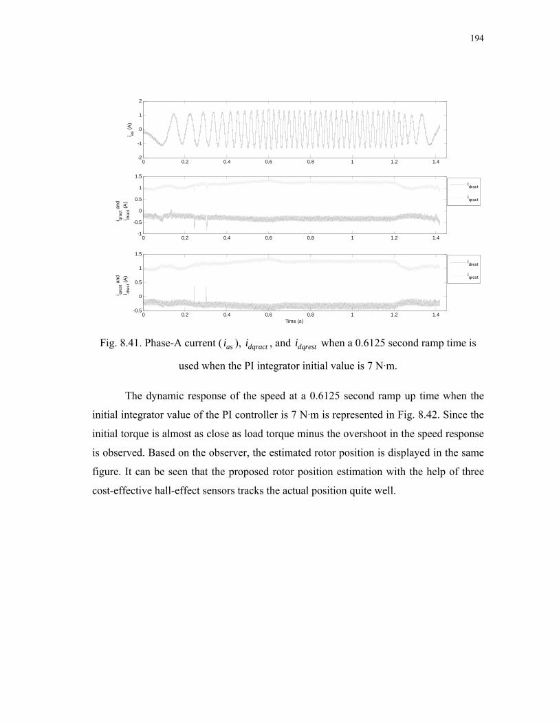
194
0 0.2 0.4 0.6 0.8 1 1.2 1.4-2
-1
0
1
2
i as (A
)
0 0.2 0.4 0.6 0.8 1 1.2 1.4-1
-0.5
0
0.5
1
1.5
i qrac
t and
i dr
act (A
)
0 0.2 0.4 0.6 0.8 1 1.2 1.4-0.5
0
0.5
1
1.5
Time (s)
i qres
t and
i dr
est (A
)
idrest
iqrest
idract
iqract
Fig. 8.41. Phase-A current ( ), , and when a 0.6125 second ramp time is
used when the PI integrator initial value is 7 N·m.
asi dqracti dqresti
The dynamic response of the speed at a 0.6125 second ramp up time when the
initial integrator value of the PI controller is 7 N·m is represented in Fig. 8.42. Since the
initial torque is almost as close as load torque minus the overshoot in the speed response
is observed. Based on the observer, the estimated rotor position is displayed in the same
figure. It can be seen that the proposed rotor position estimation with the help of three
cost-effective hall-effect sensors tracks the actual position quite well.

195
0.2 0.4 0.6 0.8 1 1.2 1.40
100
200
300
Spe
edes
t and
Spe
edre
f (rad
/sec
)
0 0.2 0.4 0.6 0.8 1 1.2 1.4-20
0
20
40
Spe
eder
r
Ref
-Act
(rad
/sec
)
0 0.2 0.4 0.6 0.8 1 1.2 1.40
2
4
6
Act
ual a
nd
Est
. Pos
ition
(rad
)
Time (s)
Fig. 8.42. Reference and actual speeds, speed error (ref-act), and actual and estimated
positions when a 0.6125 second ramp time is used when the PI integrator initial value is
7 N·m.
8.2.3.2. Effects of Stator Resistance Variation in Conventional DTC with Encoder
In order to examine the effects of the sR variations of a PM synchronous
machine, a MATLAB/SIMULINK® conventional DTC model was developed. The
DC-link voltage is set at 370 volts. The sR value in the motor model is varied by certain
amount, such as 1.5 times of the nominal value (steady-state, transient and starting etc.).
It should be noted that in all the work related to the resistance change presented here, the
transient load torque is assumed to ramp from 7 N·m to 10 N·m to mimic the real
washing machine load characteristics.
First, a conventional DTC is simulated without the stator resistance change.
Figs. 8.43 and 8.44 show the reference and actual speeds, actual position, and the three

196
phase currents, the reference and estimated electromagnetic torques and the estimated
stator flux linkage when a 0.35 second ramp up time is selected and the stator resistance
is not varied, respectively. Since no resistance change effect is applied and an encoder is
used for speed control, good results are achieved.
0 0.2 0.4 0.6 0.8 1 1.20
100
200
300
Spe
edre
f
an
d S
peed
act (r
ad/s
ec)
0 0.2 0.4 0.6 0.8 1 1.20
2
4
6
Pos
ition
Act
ual (
rad)
Actu
al P
ositi
on (r
ad)
2
0 0.2 0.4 0.6 0.8 1 1.2-2
-1
0
1
Time (s)
Thre
e ph
ase
c
urre
nts
(A)
Fig. 8.43. Reference and actual speeds, actual position, and three phase currents when a
0.35 second ramp time is used (no initial torque, just ramp rate is added). Stator
resistance change effect is not applied.

197
0 0.2 0.4 0.6 0.8 1 1.2 1.40
5
10
15
T emre
f (N.m
)
0 0.2 0.4 0.6 0.8 1 1.2 1.40
5
10
15
T emes
t (N.m
)
0 0.2 0.4 0.6 0.8 1 1.2 1.40.21
0.215
0.22
0.225
0.23
0.235
Time (s)
Flux
est (W
b)
Fig. 8.44. , , and at a 0.35 second ramp time. Stator resistance
change effect is not applied.
emrefT emestT estFlux
A mismatch between the controller set stator resistance and its actual value in the
machine can create instability as shown in Fig. 8.45. This figure shows the simulation
results for a step stator resistance change from 100% to 150% of its nominal value at
0 second and a torque command (7 N·m to 10 N·m) is applied at the start up. The drive
system becomes unstable if controller instrumented stator resistance is lower than its
actual value in the motor. This may be explained as follows: As the motor resistance
increases in the machine, then its current decreases for the same applied voltages, which
decreases the flux and electromagnetic torque. The controller has the opposite effect in
that the decreased currents, which are inputs to the system, cause decreased stator
resistance voltage drops in the calculator resulting in higher flux linkages and
electromagnetic torque estimation. They are compared with their command values
giving larger torque and flux linkages errors resulting in commanding larger voltages
and hence in larger currents leading to a run off condition. The instability result under a

198
step change is questionable as the stator resistance does not change in a step manner in
practice. From the earlier work a linearly decreasing stator resistance provided the same
result. Even for such a gradual change of stator resistance, note that the system becomes
unstable. The controller calculated electromagnetic torque and stator flux linkages are
equal to set values and contrary to the real situation in the machine. Therefore, any
scheme using these values for parameter compensation would not be effective. For
example, the airgap power feedback control for parameter compensation in an indirect
vector controlled drive system is successful but it will not work in the DTC drive
system.
0 0.2 0.4 0.6 0.8 1 1.27
8
9
10
Load
Tor
que
(N.m
)
0 0.2 0.4 0.6 0.8 1 1.2-20
0
20
T emes
t and
T emre
f (N.m
)
0 0.2 0.4 0.6 0.8 1 1.2-50
0
50
T emac
t (N.m
)
0 0.2 0.4 0.6 0.8 1 1.20.2
0.22
0.24
0.26
Flux
est (W
b)
Time (s)
Fig. 8.45. Load torque (TL), , , , and estimated stator flux linkage
under step stator resistance change (1.5x
emrefT emestT emactT
sR ) at 0 second when ramp time is 0.35 second
when the initial integrator value of the PI is chosen as 7 N·m.
Fig. 8.46 illustrates the actual and reference speeds, actual position, and three
phase motor currents. It can be seen from Fig. 8.45 that due to the lack of control of the

199
torque caused by the stator resistance mismatch, the speed control becomes unnstable
after a few milliseconds of running. If the mismatch in sR is larger, the instability occurs
earlier and vice versa.
0 0.2 0.4 0.6 0.8 1 1.2-200
-100
0
100
200
300
Spe
edre
f
an
d S
peed
act (r
ad/s
ec)
0 0.2 0.4 0.6 0.8 1 1.2
-6
-4
-2
0
2
Pos
ition
Act
ual (
rad)
Actu
al P
ositi
on (r
ad)
5
0 0.2 0.4 0.6 0.8 1 1.2-5
0
Time (s)
Thre
e ph
ase
c
urre
nts
(A)
Fig. 8.46. Reference and actual speeds, actual position, and three phase currents when a
0.35 second ramp time is used (no initial torque, just ramp rate is added). Stator
resistance is increased by 1.5x sR at 0 second (V 370dc = V).
When the stator resistance with a %50 mismatch in sR happens during the
steady-state, as shown in Fig. 8.47, the speed tracks the commanded value very well.
The problem with this, however, is that the actual motor current increases.

200
0 0.2 0.4 0.6 0.8 1 1.20
100
200
300
Spe
edre
f
an
d S
peed
act (r
ad/s
ec)
0 0.2 0.4 0.6 0.8 1 1.20
2
4
6
Pos
ition
Act
ual (
rad)
Actu
al P
ositi
on (r
ad)
0 0.2 0.4 0.6 0.8 1 1.2
-2
-1
0
1
2
Time (s)
Thre
e ph
ase
c
urre
nts
(A)
Fig. 8.47. Reference and actual speeds, actual position, and three phase currents when a
0.35 second ramp time is used (no initial torque, just ramp rate is added). Stator
resistance is increased by 1.5x sR at 0.675 second ( 370dcV = V).
When the stator resistance is increased, the estimated and reference
electromagnetic torque values also increase while the stator flux linkage estimation
remains constant, as depicted in Fig. 8.48.

201
0 0.2 0.4 0.6 0.8 1 1.20
5
10
15
20
T emre
f (N.m
)
0 0.2 0.4 0.6 0.8 1 1.20
5
10
15
20
T emes
t (N.m
)
0 0.2 0.4 0.6 0.8 1 1.20.21
0.215
0.22
0.225
0.23
0.235
Flux
est (W
b)
Time (s)
Fig. 8.48. , , and at a 0.35 second ramp time. Stator resistance is
increased by 1.5x
emrefT emestT estFlux
sR at 0.675 second ( 370dcV = V).
Fig. 8.49 illustrates a good comparison between the estimated electromagnetic
torque, the estimated stator flux linkage value, the actual electromagnetic torque and the
actual stator flux linkage value, respectively. When the resistance increases during
steady-state, the actual value of the electromagnetic torque increases but the actual stator
flux linkage value decreases.

202
0 0.2 0.4 0.6 0.8 1 1.2-5
0
5
10
15
20
T emac
t and
T em
est (N
.m)
0 0.2 0.4 0.6 0.8 1 1.20
0.05
0.1
0.15
0.2
0.25
Flux
act a
nd
Flux
est (W
b)
0 0.2 0.4 0.6 0.8 1 1.2-4
-2
0
2
4
Time (s)
Pos
ition
act a
nd
Pos
ition
est (r
ad)
Temact
Fluxact
Fig. 8.49. , , , , estimated and real rotor positions with a
0.35 second ramp time. Stator resistance is increased by 1.5x
emestT emactT estFlux actFlux
sR at 0.675 second
( 370dcV = V).
Since washing machine agitation speed control needs to work back and forth
between zero and the plateau speed quickly, the resistance change effect will also be
observed in the transient as well as in the start up, even though the change happens in
steady-state. The simulation results show that the change in the stator resistance during
the transient state causes more devastating results in the closed loop speed control, even
with an encoder. Fig. 8.50 shows the electromagnetic torque and the stator flux linkage
behavior of the motor when resistance is incremented by 50% of its nominal value at
0.35/2 second. After a few milliseconds the motor torque becomes unstable which makes
the flux linkage and speed control go unstable. As soon as the step change in the stator
resistance occurs at the transient state the speed goes unstable as shown in Fig. 8.51. As
discussed earlier in this section, in reality the resistance will not change as a step change,
it changes gradually. Recent simulation tests conducted by some authors claim that the

203
gradual change in resistance will only prolong the period of time before instability
occurs.
0 0.2 0.4 0.6 0.8 1 1.2-40
-20
0
20
40
T emac
t and
T em
est (N
.m)
0 0.2 0.4 0.6 0.8 1 1.20
0.1
0.2
0.3
0.4
0.5
Flux
act a
nd
Flux
est (W
b)
0 0.2 0.4 0.6 0.8 1 1.2-4
-2
0
2
4
Pos
ition
act a
nd
Pos
ition
est (r
ad)
Time (s)
Temest
Fluxact
Fluxest
Fig. 8.50. , , , , estimated and real rotor positions with a
0.35 second ramp time. Stator resistance is increased by 1.5x
emestT emactT estFlux actFlux
sR at 0.35/2 second
( 370dcV = V).

204
0 0.05 0.1 0.15 0.2 0.25-50
0
50
100
150
200
Spe
edre
f
an
d S
peed
act (r
ad/s
ec)
0 0.05 0.1 0.15 0.2 0.250
2
4
6
Pos
ition
Act
ual (
rad)
Actu
al P
ositi
on (r
ad)
0 0.05 0.1 0.15 0.2 0.25
-2
-1
0
1
2
Thre
e ph
ase
c
urre
nts
(A)
Time (s)
Fig. 8.51. Reference and actual speeds, actual position, and three phase currents when a
0.35 second ramp time is used (no initial torque, just ramp rate is added). Stator
resistance is increased by 1.5x sR at 0.35/2 second ( 370dcV = V).

205
0 0.05 0.1 0.15 0.2 0.250
5
10
15
20
T emre
f (N.m
)
0 0.05 0.1 0.15 0.2 0.250
5
10
15
20
T emes
t (N.m
)
0 0.05 0.1 0.15 0.2 0.250.21
0.215
0.22
0.225
0.23
0.235
Flux
est (W
b)
Time (s)
Fig. 8.52. , , and with a 0.35 second ramp time. Stator resistance is
increased by 1.5x
emrefT emestT estFlux
sR at 0.35/2 second ( 370dcV = V).
Fig. 8.53 illustrates the estimated stator flux linkage circular trajectory when the
stator resistance is increased by 50% of its nominal value at steady state. The
proportional coefficient of the speed in PI controller is chosen as 9 and the integral
coefficient as 3 for all the simulation that are run.

206
Fig. 8.53. Estimated sDλ (X axis) and sQλ (Y axis) circular trajectory with a 0.35 second
ramp time. Stator resistance is increased by 1.5x sR at 0.675 second (kp=9, ki=3).
The estimated stator flux linkage trajectory when the stator resistance value is
step changed at 0.35/2 second is given in Fig. 8.54. It can clearly be seen that the
resistance value changed in the transient state causes the stator flux linkage locus to be
less smooth than the change occuring at steady-state depicted in Fig. 8.53.

207
Fig. 8.54. Estimated sDλ (X axis) and sQλ (Y axis) circular trajectory with a 0.35 second
ramp time. Stator resistance is increased by 1.5x sR at 0.35/2 second (kp=9, ki=3).
The actual stator flux linkage locus when resistance is varied at the transient state
(0.35/2 second) is shown in Fig. 8.55. Unlike the estimated flux linkage, the actual value
of the stator flux linkage is out of the circular trajectory limit. In this case, the simulation
is stopped at 0.28 second to let the deviation in the flux linkage locus be seen clearly.

208
Fig. 8.55. Actual sDλ (X axis) and sQλ (Y axis) circular trajectory with a 0.35 second
ramp time. Stator resistance is increased by 1.5x sR at 0.35/2 second (stopped at 0.28 s.).
When the stator resistance is changed at steady-state, the circular trajectory
becomes smaller as shown in Fig. 8.56. This occurs when the stator resistance is
increased during the transient state. It has been observed that much quick instability
occurs in the speed control when the stator resistance varies during the transient state
compared to stator resistance varies during steady-state. If the application lets the motor
start once and runs at steady-state then most of the time less instability may be observed
because of the stator resistance change effect. On the other hand, in the washing machine
speed control, the speed has zero, transient, and steady-state conditions such that the
change in stator resistance can occur at any time. This is so that worse case (transient
state) scenario can be considered.

209
Fig. 8.56. Actual sDλ (X axis) and sQλ (Y axis) circular trajectory with a 0.35 second
ramp time. Stator resistance is increased by 1.5x sR at 0.675 second (stopped at 0.28 s.)
8.2.3.3. Drift Problem Occurs in Conventional DTC Scheme
The stator flux is estimated in DTC by integrating the difference between the
input voltage and the voltage drop across the stator resistance. When the stator flux is
indirectly estimated from the integration of the back-EMF, any DC-offset is also
integrated and would eventually lead to large drifts in the stator flux linkage. Operational
amplifiers are normally used to amplify the signal from the current and voltage sensors.
These sensors have a temperature dependent DC-offset. Since the current measurement
path contains many analog devices, DC-offset is an inevitable problem. The error in the
stator flux estimation also causes an error in the torque estimation, so the drive system
may become unstable [35].
The scaling error is another type of current measurement error. Stator currents
are transformed to the voltage signal by current sensors and are transformed into digital
values via low pass filters and A/D converters. The output of a current sensor must be

210
scaled to fit the input range of an A/D converter to get the real value of a current. During
this process, some scaling error may be introduced. Obviously, drift compensation is an
important factor in a practical implementation of the integration, since drift can cause a
large error in the estimated flux linkage. The error in the estimated flux linkage can
cause error in the estimated torque and speed [35].
Figs. 8.57 through 8.59 show the experimental results when a 0.1 A (~ 4% of the
rated current) offset is introduced. Figure 8.57 shows the reference and actual speeds and
the actual position and three phase motor currents with an offset added. It is seen that the
speed quickly goes unstable at start up and the accumulation of the offset error causes
the estimated stator flux to drift from its origin as shown in Fig. 8.59. Fig. 8.58 shows
the load torque, the reference and actual electromagnetic torque and also the reference
and actual stator flux linkages. Starting at 0.4 second, the stator flux linkage oscillates
too much and its amplitude increases greatly and from around 0.5 second the actual
developed torque oscillates and in a short time goes unstable (not shown in the figure).

211
0 0.1 0.2 0.3 0.4 0.5 0.6-3000
-2000
-1000
0
1000
Spe
edre
f
an
d S
peed
act (r
ad/s
)
0 0.1 0.2 0.3 0.4 0.5 0.6-10
-5
0
5
Pos
ition
Act
ual (
rad)
0 0.1 0.2 0.3 0.4 0.5 0.6-10
-5
0
5
10
Time (s)
Thre
e ph
ase
c
urre
nts
(A)
Speedref (rad/s)
Fig. 8.57. Reference and actual speeds, actual position, and three phase currents when a
0.35 second ramp time is used (no initial torque, just ramp rate is added). A 0.1 A
current offset is added to the D- and Q-axes currents in the SRF ( V). 370dcV =
Actu
al P
ositi
on (r
ad)

212
0 0.1 0.2 0.3 0.4 0.5 0.67
8
9
10
Load
Tor
que
(N.m
)
0 0.1 0.2 0.3 0.4 0.5 0.6-50
0
50
T emre
f (N.m
)
0 0.1 0.2 0.3 0.4 0.5 0.6-50
0
50
T emac
t (N.m
)
0 0.1 0.2 0.3 0.4 0.5 0.60.2
0.4
0.6
0.8
Time (s)
Flux
act a
nd
Flux
est (W
b) Fluxact
Fig. 8.58. Load torque (TL), , , , and actual stator flux linkage.
A 0.1 A offset occurs on the D- and Q-axes currents in the SRF when the ramp time is
0.35 second.
emrefT emactT estFlux

213
Fig. 8.59. Estimated sDλ (X axis) and sQλ (Y axis) circular trajectory with a 0.35 second
ramp time. A 0.1 A offset is included in the D- and Q-axes currents in the SRF
( 37dcV 0= V). (kp=9, ki=3).
8.2.3.4. Overview of the Offset Error Occurred in the Proposed DTC Scheme
Unlike the conventional DTC scheme, the test results shown below prove that
around a 4% offset in the d- and q-axes currents in the RRF does not affect the
closed-loop speed control of the proposed DTC scheme. When there is an initial 7 N·m
load torque in the washing machine which gradually increases to a 10 N·m steady-state
limit proportional to the speed (choosing 7.5 N·m. initial integrator value in the speed PI
controller) results in smooth starting in the case of an offset added to the currents. If a
7 N·m initial value is selected, a lower smoothness in the speed response is observed.
Since the adaptive initial value correction algorithm (discussed earlier in this section) is
used, after a few strokes the right value would be reached even if there is an offset in the
measurement systems.

214
Figs. 8.60 to 8.64 display several simulation results when a 0.1 A offset error is included
to the d- and q-axes currents in the RRF. Similar behaviors are observed in the results
without the offset error discussed earlier in this section.
0 0.2 0.4 0.6 0.8 1 1.20
100
200
300
Spe
edes
t and
Spe
edre
f (rad
/s)
0 0.2 0.4 0.6 0.8 1 1.2-20
0
20
40
Spe
eder
r
Ref
-Act
(rad
/s)
0 0.2 0.4 0.6 0.8 1 1.20
2
4
6
Act
ual a
nd
Est
. Pos
ition
(rad
)
Time (s)
Fig. 8.60. Reference and actual speeds, speed error (ref-act), estimated and actual
positions when a 0.35 second ramp time is used (7.5 N·m initial torque is used in the PI’s
integrator with appropriate ramp rate). A 0.1 A offset is included in the d- and q-axes
currents in the RRF ( 370dcV = V).

215
0 0.2 0.4 0.6 0.8 1 1.2-2
-1
0
1
2
i as (A
)
0 0.2 0.4 0.6 0.8 1 1.2-2
-1
0
1
2
i qrac
t and
i dr
act (A
)
0 0.2 0.4 0.6 0.8 1 1.2-1
0
1
2
i qres
t and
i dr
est (A
)
Time (s)
idract
iqract
idrest
iqrest
Fig. 8.61. Phase-A current ( ), , and when a 0.35 second ramp time is used
with a PI integrator initial value of 7.5 N·m. A 0.1 A offset is included in the d- and
q-axes current in the RRF (
asi dqracti dqresti
370dcV = V).

216
0 0.2 0.4 0.6 0.8 1 1.27
8
9
10
Load
Tor
que
(N.m
)
0 0.2 0.4 0.6 0.8 1 1.20
5
10
15
T emre
f (N.m
)
0 0.2 0.4 0.6 0.8 1 1.20
5
10
15
T emes
t (N.m
)
0 0.2 0.4 0.6 0.8 1 1.20
5
10
15
T emac
t (N.m
)
Time (s)
Fig. 8.62. Load torque (TL), , , and . A 0.1 A offset occurs on d- and
q-axes currents in the RRF when ramp time is 0.35 second ( V).
emrefT emestT emactT
370dcV =
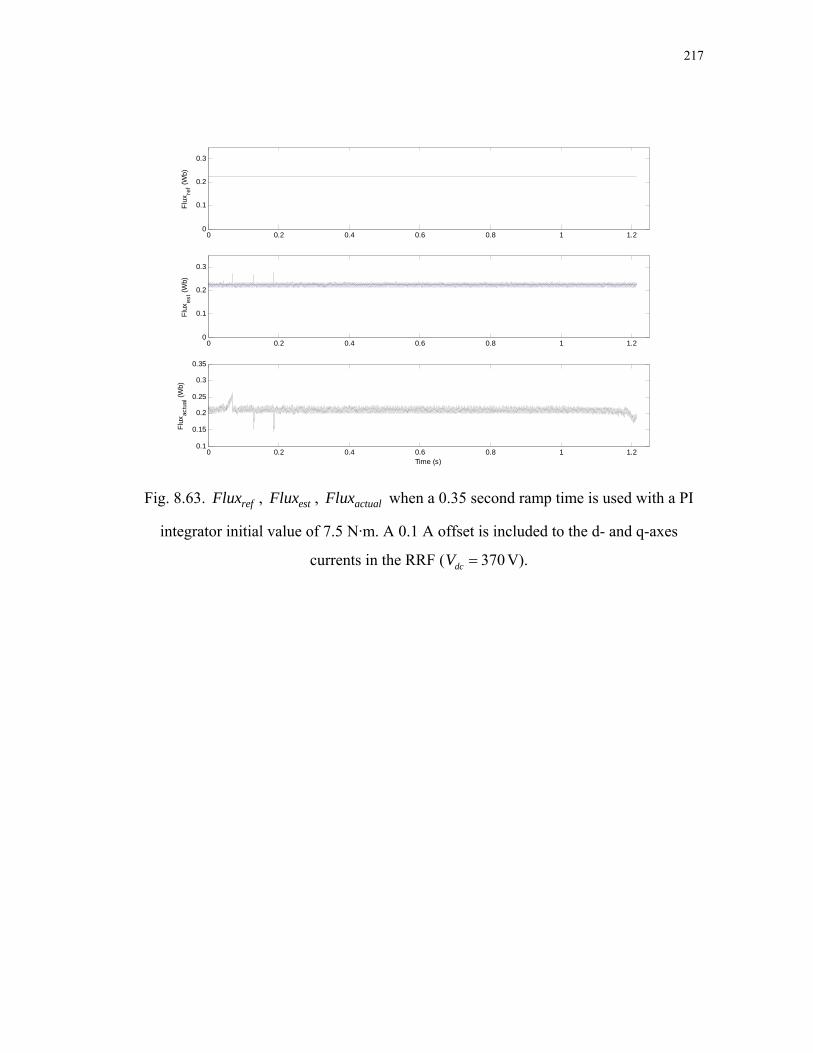
217
0 0.2 0.4 0.6 0.8 1 1.20
0.1
0.2
0.3
Flux
ref (W
b)
0 0.2 0.4 0.6 0.8 1 1.20
0.1
0.2
0.3
Flux
est (W
b)
0 0.2 0.4 0.6 0.8 1 1.20.1
0.15
0.2
0.25
0.3
0.35
Time (s)
Flux
actu
al (W
b)
Fig. 8.63. , , when a 0.35 second ramp time is used with a PI
integrator initial value of 7.5 N·m. A 0.1 A offset is included to the d- and q-axes
currents in the RRF (
refFlux estFlux actualFlux
370dcV = V).

218
Fig. 8.64. Estimated sDλ (X axis) and sQλ (Y axis) circular trajectory at a 0.35 second
ramp time with a PI integrator initial value of 7.5 N·m. A 0.1 A offset is included in the
d- and q-axes currents in the RRF ( 370dcV = V). (kp=9, ki=3).
8.2.3.5. Overview of the Rotor Flux Linkage Error Occurred in the Proposed DTC
Scheme
Similar to conventional the DTC scheme having sR variations due to temperature
change and low the speed effect, in the proposed scheme the rotor flux linkage value is
considered as constant in most of the cases. The exception to this is in high temperature
conditions. Some experiments show that amplitude of the rotor flux linkage can vary up
to 20-30 percent of its nominal value at around 100 C° on the motor stator windings. The
value of the rotor flux linkage amplitude decreases when temperature rises. Several
simulations are conducted to examine the effect of the rotor flux linkage change effect
when the motor heats up on the closed-loop control of the proposed DTC scheme. The
rotor flux linkage amplitude is step changed when the motor speeds up (at
0.35/2 second) proportional to the load torque. This is considered the worse case

219
situation. The results, however, prove that the 30% decrease in the rotor flux linkage
amplitude does not have a large impact on the closed-loop speed control.
Some of the simulation results when the rotor flux linkage value is changed by
70% of its nominal value are given from Figs. 8.65 through 8.69.
0 0.2 0.4 0.6 0.8 1 1.20
100
200
300
Spe
edes
t and
Spe
edre
f (rad
/s)
0 0.2 0.4 0.6 0.8 1 1.2-20
0
20
40
Spe
eder
r
Ref
-Act
(rad
/s)
0 0.2 0.4 0.6 0.8 1 1.20
2
4
6
Act
ual a
nd
Est
. Pos
ition
(rad
)
Time (s)
Fig. 8.65. Reference and actual speeds, speed error (ref-act), estimated and actual
positions when a 0.35 second ramp time is used (7 N·m. initial torque is used in the PI’s
integrator with appropriate ramp rate). 0.7x is used at 0.35/2 second in the motor
model (
rλ
370dcV = V). (kp=9, ki=3).

220
0 0.2 0.4 0.6 0.8 1 1.2-2
-1
0
1
2
i as (A
)
0 0.2 0.4 0.6 0.8 1 1.2-1
-0.5
0
0.5
1
1.5
i qrac
t and
i dr
act (A
)
0 0.2 0.4 0.6 0.8 1 1.2-1
0
1
2
i qres
t and
i dr
est (A
)
Time (s)
Fig. 8.66. Phase-A current ( ), , and when a 0.35 second ramp time is used
with a PI integrator initial value of 7 N·m. 0.7x is used at 0.35/2 second in the motor
model (
asi dqracti dqresti
rλ
370dcV = V). (kp=9, ki=3).

221
0 0.2 0.4 0.6 0.8 1 1.27
8
9
10
Load
Tor
que
(N.m
)
0 0.2 0.4 0.6 0.8 1 1.20
5
10
15
T emre
f (N.m
)
0 0.2 0.4 0.6 0.8 1 1.20
5
10
15
T emes
t (N.m
)
0 0.2 0.4 0.6 0.8 1 1.20
5
10
15
T emac
t (N.m
)
Time (s)
Fig. 8.67. Load torque (TL), , , and . 0.7x is used at 0.35/2 second in
the motor model (
emrefT emestT emactT rλ
370dcV = V). (kp=9, ki=3).
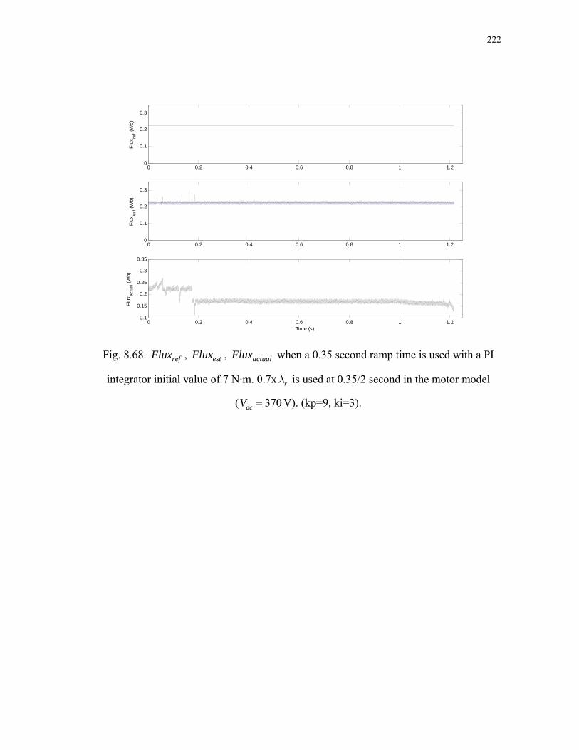
222
0 0.2 0.4 0.6 0.8 1 1.20
0.1
0.2
0.3
Flux
ref (W
b)
0 0.2 0.4 0.6 0.8 1 1.20
0.1
0.2
0.3
Flux
est (W
b)
0 0.2 0.4 0.6 0.8 1 1.20.1
0.15
0.2
0.25
0.3
0.35
Time (s)
Flux
actu
al (W
b)
Fig. 8.68. , , when a 0.35 second ramp time is used with a PI
integrator initial value of 7 N·m. 0.7x is used at 0.35/2 second in the motor model
( 3
refFlux estFlux actualFlux
rλ
7dcV 0= V). (kp=9, ki=3).
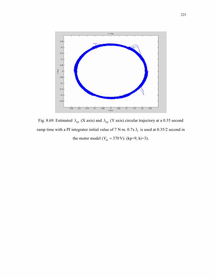
223
Fig. 8.69. Estimated sDλ (X axis) and sQλ (Y axis) circular trajectory at a 0.35 second
ramp time with a PI integrator initial value of 7 N·m. 0.7x is used at 0.35/2 second in
the motor model (
rλ
370dcV = V). (kp=9, ki=3).

224
CHAPTER IX
SUMMARY AND FUTURE WORK
9.1. Summary of the Work and Conclusion
The primary contribution of this thesis work is the development, analysis and
simulation verification of DTC of PMSM algorithm using three hall-effect sensors that is
based on rotor reference frame topology for the improvement of the commercial
top-loaded laundry washing machine agitation speed control system.
Since DTC scheme is often categorized as a sensorless torque control technique
because stator flux linkage and electromagnetic torque can easily be estimated without a
mechanical position or speed sensor at all but very low speeds. At very low and zero
speeds, the technique suffers the same performance degradation as any sensorless
method that is based on back-EMF integration. At very low speeds the back-EMF
information is very weak and quietly comparable with the supply voltage in addition of
resistance variation in conjunction with current and voltage sensing errors (offset errors
causing a drift in integration). On the other hand, since proposed method does not use
any integration (back-EMF integration), and uses the rotor position information which is
updated at every 60 electrical degrees by the help of three cost-effective hall-effect
sensors very low speed control is performed without any problem unlike basic DTC
scheme.
Observer based type of position estimation techniques have problem of
accumulating the position errors. Hall-effect sensor correction method gives a solution
for these problems. By correcting the estimated position every cycle, no compensation
algorithm is required and accumulating error is also eliminated.

225
This method eliminates the need of back-EMF integration to estimate the stator
flux linkage; instead, rotor reference frame solution which relies only on the parameters
of rotor flux linkage amplitude and dq-axis synchronous inductances rather than more
sensitive stator resistance used in basic DTC scheme, is proposed for the same purpose.
First, the mathematical basis of the developed method is derived and explained in detail
then simulation model is built in MATLAB/SIMULINK® to verify the proposed method
both in transient and steady-state condition with transient load starting from 7 N·m at
start up and increase up to 10 N·m proportional to speed and the results are given and are
discussed. As it can be seen in Section 8.2.3 of Chapter VIII, results of the simulations
verify the feasibility of the proposed control scheme over the commercialized one. One
conclusion can be drawn from the results is that the proposed method shows superior
speed and torque responds when compare with the commercial agitate speed control
system. Comparing to conventional DTC scheme when it has resistance variations and
offset error causing drift in the stator flux linkage and eventually the instability in
closed-loop speed control, those effects are included to the proposed DTC scheme also
but no speed or torque instability are noted. Instead of resistance variation, rotor flux
linkage amplitude is varied in the proposed DTC topology because only two motor
parameters (rotor flux linkage amplitude and synchronous inductance) are used in the
scheme.
9.2. Future Work
More work could be done in the future to improve the DTC of PMSM drive in
both quality and economical manner. Some of those possible works are listed below:
• Current sensorless technique can be considered.
• Parameter change effect and their compensation can be included.

226
• Current model used in this thesis can be combined with voltage model to
improve the performance of the speed control.
• One of the efficient ways of sensorless control techniques, high frequency
injection, can be implemented.
• One and/or two hall-effect sensors instead of three can be used.
• Saturation effect on the synchronous inductance can be included.
• Temperature arise impacting on rotor flux linkage amplitude can be
studied.

227
REFERENCES
[1] A. Khurram, “Position and speed sensorless control of permanent magnet synchronous motors.” Ph.D. dissertation, Michigan State University, East Lansing, MI, 2001.
[2] P. Vas. Vector Control of AC Machines. London, U.K.: Oxford Univ. Press, 1990.
[3] R.V. Khopkar, “DC-DC converter current source fed naturally commutated brushless DC motor drive.” M.S. thesis, Texas A&M University, College Station, TX, 2003.
[4] V. Valkenburg and Nooger & Neville, Inc. Basic Electricity, Revised ed. Indianapolis, IN: PROMPT Pub., 1992.
[5] G. Rizzoni. Principles and Application of Electrical Engineering, Revised 4th ed. New York, NY: McGraw-Hill Publishing Company, 2004.
[6] J. Luukko, “Direct torque control of permanent magnet synchronous machines - analysis and implementation.” Ph.D. dissertation, Lappeenranta University of Technology, Lappeenranta , Finland, 2000.
[7] T. Kim, “Sensorless control of the BLDC motors from near-zero to full speed.” Ph.D. dissertation, Texas A&M University, College Station, TX, 2001.
[8] L. Hao, “Permanent magnet AC motor full speed range operation using hybrid sliding mode observer.” Ph.D. dissertation, Texas A&M University, College Station, TX, 2002.
[9] D.Y. Ohm, “Dynamic model of PM synchronous motors,” Drivetech, Inc., Blacksburg, Virginia. www.drivetech.com.
[10] C.M. Ong. Dynamic Simulation of Electric Machinery Using MATLAB / SIMULINK. Upper Saddle River, NJ: Prentice Hall PTR, 1998.
[11] P. Yedamale, “Brushless DC (BLDC) Motor Fundamentals,” Application Note 885, Microchip Technology Inc., Chandler, AZ, 2003.
[12] P. Pillay, “Modeling simulation and analysis of permanent magnet synchronous and brushless DC motor drives.” Ph.D. dissertation, Virginia Polytechnic Institute and State University, Blacksburg, VI, 1987.
228
[13] S.P.Waikar, “A low-cost low-loss brushless permanent magnet motor drive.” Ph.D. dissertation, Texas A&M University, College Station, TX, 2001.
[14] D. Y. Ohm and J. H. Park, “About commutation and current control methods for brushless motors,” 28th Annual Symposium on Incremental Motion Control Systems and Devices, San Jose, CA. July 26-29, 1999.
[15] B.K. Bose. Power Electronics and Variable Frequency Drives - Technology and Application. Piscataway, NJ: IEEE Press, 1997.
[16] P. Vas, Sensorless Vector and Direct Torque Control. London, U.K.: Oxford Univ. Press, 1998.
[17] J.R. Hendershot Jr and T.J.E. Miller. Design of Brushless Permanent-Magnet Motors. Oxford, U.K.: Magna Physics/Clarendon, 1994.
[18] K. Hasse, “Drehzahlgelverfahren für schnelle umkehrantriebe mit stromrichtergespeisten asynchron-kurzschlusslaufer-motoren,” Reglungstechnik, vol. 20, pp. 60–66, 1972.
[19] I. Takahashi and T. Noguchi, “A new quick-response and high efficiency control strategy of an induction machine,” IEEE Trans. Ind. Appl., vol. IA-22, pp. 820–827, Sept./Oct. 1986.
[20] U. Baader, M. Depenbrock, and G. Gierse, “Direct self control (DSC) of inverter-fed-induction machine—A basis for speed control without speed measurement,” IEEE Trans. Ind. Appl., vol. 28, pp. 581–588, May/June 1992.
[21] M. Depenbrock, “Direct self control of inverter-fed induction machines,” IEEE Trans. Power Electron., vol. 3, pp. 420–429, Oct. 1988.
[22] M. Depenbrock, “Direct self-control of the flux and rotary moment of a rotary-field machine,” U.S. Patent 4 678 248, July 7, 1987.
[23] C. French and P. Acarnley, “Direct torque control of permanent magnet drives,” IEEE Trans. Ind. Appl., vol. IA-32, pp. 1080–1088, Sept./Oct. 1996.
[24] L. Zhong, M. F. Rahman, W. Y. Hu, and K. W. Lim, “Analysis of direct torque control in permanent magnet synchronous motor drives,” IEEE Trans. Power Electron., vol. 12, pp. 528–536, May 1997.
[25] I. Takahashi and T. Noguchi, “Take a look back upon the past decade of direct torque control,” in Proc. IEEE-IECON’97 23rd Int. Conf., vol. 2, 1997, pp. 546–551.

229
[26] D. Casadei, G. Serra, and A. Tani, “Implementation of a direct torque control algorithm for induction motors based on discrete space vector modulation,” IEEE Trans. Power Electron., vol. 15, pp. 769–777, July 2000.
[27] C. G. Mei, S. K. Panda, J. X. Xu, and K. W. Lim, “Direct torque control of induction motor-variable switching sectors,” in Proc. IEEE-PEDS Conf., Hong Kong, July 1999, pp. 80–85.
[28] A. Tripathi, A. M. Khambadkone, and S. K. Panda, “Space-vector based, constant frequency, direct torque control and dead beat stator flux control of AC machines,” in Proc. IEEE-IECON’01 Conf., Nov. 2001, pp. 1219–1224.
[29] C. Lascu, I. Boldea, and F. Blaabjerg, “A modified direct torque control for induction motor sensorless drive,” IEEE Trans. Ind. Appl., vol. 36, pp. 122–130, Jan./Feb. 2000.
[30] D. Swierczynski, M. Kazmierkowski, and F. Blaabjerg, “DSP based direct torque control of permanent magnet synchronous motor (PMSM) using space vector modulation (DTC-SVM),” in Proc. IEEE Int. Symp. Ind. Electron., vol. 3, May 2002, pp. 723–727.
[31] L. Tang , L. Zhong, M. F. Rahman, and Y. Hu “A novel direct torque control for interior permanent-magnet synchronous machine drive with low ripple in torque and flux-a speed-sensorless approach,” in Proc. IEEE Trans. Ind. Appl., vol. 39, pp. 1748–1756, Nov/Dec 2003.
[32] C. Martins, X. Roboam, T. A. Meynard, and A. S. Caryalho, “Switching frequency imposition and ripple reduction in DTC drives by using a multilevel converter,” IEEE Trans. Power Electron., vol. 17, pp. 286–297, Mar. 2002.
[33] Y. A. Chapuis, D. Roye, and J. Davoine, “Principles and implementation of direct torque control by stator flux orientation of an induction motor,” in Conf. Rec. IEEE-IAS Annu. Meeting, vol. 1, 1995, pp. 185–191.
[34] B. K. B. And and N. R. Patel, “A programmable cascaded low-pass filter-based flux synthesis for a stator flux-oriented vector-controlled induction motor drive,” IEEE Trans. Ind. Electron., vol. 44, pp. 140–143, Feb. 1997.
[35] M. R. Zolghadri and D. Roye, “A fully digital sensorless direct torque control system for synchronous machine,” Elect. Mach. Power Syst., vol. 26, pp. 709–721, 1998.

230
[36] M.F. Rahman, Md. E. Haque, L. Tang, and L. Zhong, “Problems associated with the direct torque control of an interior permanent-magnet synchronous motor drive and their remedies,” IEEE Trans. Ind. Electronics., vol. 51, pp. 799–809, August 2004.
[37] S. Mir, M. E. Elbuluk, and D. S. Zinger, “PI and fuzzy estimators for tuning the stator resistance in direct torque control of induction machines,” IEEE Trans. Power Electron., vol. 13, pp. 279–287, Mar. 1998.
[38] L. Zhong, M. F. Rahman, K. W. Lim, Y. Hu, and Y. Xu, “A fuzzy observer for induction motor stator resistance for application in direct torque control,” in Conf. Rec. IEEE Power Electronics and Drive Systems Conf., 1997, pp. 91–96.
[39] B. S. Lee and R. Krishnan, “Adaptive stator resistance compensator for high performance direct torque controlled induction motor drive,” in Conf. Rec. IEEE-IAS Annu. Meeting, St. Louis, MO, 1998, pp. 423–423.
[40] M. E. Haque and M. F. Rahman, “Influence of stator resistance variation on direct torque controlled interior permanent magnet synchronous motor drive performance and its compensation,” in Conf. Rec. IEEE-IAS Annu. Meeting, 2001, pp. 2563–2569.
[41] R. Dhaouadi, N. Mohan, and L. Norum, “Design and implementation of an extended Kalman filter for the state estimation of a permanent magnet synchronous motor,” IEEE Trans. Power Electron., vol. 6, no. 3, pp. 491–497, 1991.
[42] M. Schroedl, “Sensorless control of AC machines at low speed and standstill based on the “INFORM” method,” in Conf. Rec. IEEE-IAS Annu. Meeting, San Diego, CA, Oct. 6–10, 1996, pp. 270–277.
[43] M. Schroedl, “Sensorless control of permanent magnet synchronous motors,” Elect. Mach. Power Syst., vol. 22, no. 2, pp. 173–185, Mar./Apr. 1994.
[44] R. B. Sepe and J. H. Lang, “Real-Time observer-based (adaptive) control of a permanent-magnet synchronous motor without mechanical sensors,” IEEE Trans. Ind. Appl., vol. 28, pp. 1345–1352, Nov./Dec. 1992.
[45] A. B. Kulkarni and M. Ehsani, “A novel position sensor elimination technique for the interior permanent magnet synchronous motor drive,” IEEE Trans. Ind. Appl., vol. 28, pp. 144–150, Jan./Feb. 1992.
[46] S. Ogasawara and H. Akagi, “An approach to real time position estimation at zero and low speed for a PM motor based on saliency,” in Conf. Rec. IEEE-IAS Annu. Meeting, San Diego, CA, Oct. 6–10, 1996, pp. 29–35.

231
[47] S. Ostlund and M. Brokemper, “Sensorless rotor-position detection from zero to rated speed for an integratedPM synchronous motor drive,” IEEE Trans. Ind. Appl., vol. 32, pp. 1158–1165, Sept./Oct. 1996.
[48] P. B. Schmidt, M. L. Gasperi, G. Ray, and A. H. Wijenayake, “Initial rotor angle detection of a nonsalient pole permanent magnet synchronous machine,” in Conf. Rec. IEEE-IAS Annu. Meeting, New Orleans, LA, Oct. 5–9, 1997, pp. 549–463.
[49] T. Noguchi, K. Yamada, S. Kondo, and I. Takahashi, “Initial rotor position estimation method of sensorless PM motor with no sensitivity to armature resistance,” IEEE Trans. Ind. Electron., vol. 45, pp. 118–125, Feb. 1998.
[50] M. W. Degner and R. D. Lorenz, “Using multiple saliencies for the estimation of flux, position, and velocity in AC machines,” in Conf. Rec. IEEE-IAS Annu. Meeting, New Orleans, LA, Oct. 5–9, 1997, pp. 760–767.
[51] M. J. Corley and R. D. Lorenz, “Rotor position and velocity estimation for a salient-pole permanent magnet synchronous machine at standstill and high speeds,” IEEE Trans. Ind. Appl., vol. 34, pp. 784–789, July/Aug. 1998.
[52] A. Consoli, G. Scarcella, and A. Testa, “Sensorless control of AC motors at zero speed,” in Proc. IEEE ISIE, vol. 1, Bled, Slovenia, July 1999, pp. 373–379.
[53] B.K. Bose. Modern Power Electronics and AC Drives. Upper Saddle River, NJ: Prentice Hall PTR., 2002.
[54] S. Morimoto, M. Sanada and Y. Takeda, “High performance current-sensorless drive for PMSM and SynRM with only low resolution position sensor,” IEEE Trans. Ind. Appl., vol. 39, no. 3, pp. 792-801 May/June 2003.
[55] J. Bu, L. Xu, T. Sebastian and B. Liu, “Near-zero speed performance enhancement of PM synchronous machines assisted by low cost hall effect sensors,” in Proc. IEEE APEC’98, 1998, pp. 68-74.
[56] D.J. Ensor, “Acceleration controller for laundry machine motor.” U.S. Patent 5,398,298, March 14, 1995.
[57] G.D. Duncan, “Electronic motor controls, laundry machines including such controls and/or methods of operating such controls.” U. S. Patent RE37,360E, September 11, 2001.
[58] J.D. Harwood, “Agitation period control of laundry machine Motor.” U.S. Patent 5,726,546, March 10, 1998.

232
APPENDIX A
Fig. A-1. Specifications of the Fujitsu MB907462A microcontroller.

233
Fig A-1. (continued).

234
Fig. A-2. Theoretical background of active power, apparent power, power factor and
connection of the power analyzer to the load (motor).

235
D
TC o
f IPM
SM w
ith 3
Hal
l-Effe
ct S
enso
rs
Lam
bda_
s*
0-1-
2-3-
4-5-
6-7
Ram
p_sp
eed_
ref
f(u)
rem
func
.
0
lam
bda_
s*
1 s 1 s
Zero
-Ord
erHo
ld fo
r wre
[D]
Wre
f_el
ec
Sw_k
s
Vas
Vbs
Vcs
Volt
Sour
ce
Vol.
Vect
or M
atrix
trq sec
phi
vect
or
Vect
or S
elec
tion
Torq
uePl
ot
Torq
uehy
stere
sisco
ntro
ller
0
Tem
_estTL
TL_S
tep_
up_d
own
Switc
h
Info
rho
sect
or1
Sect
or F
inde
r
100*
2*pi
/60*
24
Ref_
elec
_ste
ady-
state
_spe
ed
Ram
p
MAT
LAB
Func
tion
Prop
osed
Alg
orith
m
0
Posit
ion(
0-2p
i)
0
Posit
ion
du/d
t
Pos-t
o-wr
e
err.
Te*
PI c
ontro
ller
Mot
or_C
urre
nts
p/2
Mec
h_to
_ele
c
Lam
bda_
s_es
t
1/Je
q
Iner
tia
va vb vc Wm
ech
thet
ar_e
st
ia ib ic
Tem
_act
ual
Lam
da_s
Tem
_est
IPM
SMM
ODE
L
[C]
Got
o2
Flux
Plot
Flux
hyste
resis
cont
rolle
r
0
Est_
elec
_spe
ed
Est_
elec
_pos
(0-2
pi)
Elec
_spe
eds
em
Dec
-Bin
Bin-
Vec
Dec2
Vec
fl_s_
0
Cloc
k2
0
Cloc
k
0
Actu
al_w
re
Actu
al_m
ech_
spee
d
Actu
al_e
lec_
pos (
0-2p
i) Ac
tual
_ele
c_po
s
0
Wm
ech
Tem
*
Fig.
A-3
. MA
TLA
B/S
IMU
LIN
K®
mod
el o
f the
pro
pose
d D
TC.

236
MOTOR PARAMETERS
p (number of poles) : 48
ratedV : 325 V
peakI : 3.5 A
2r kλ = e (rotor flux linkage): 0.223256 Vs/rad
sR : 16.30983 Ω
sL : 61.8183 mH
d qL L= : 92.72745 mH
peakT : 30 N·m

237
VITA
Salih Baris Ozturk received his Bachelor of Science degree from Istanbul
Technical University, Istanbul, Turkey, in June 2000. He worked in the Electrical
Machines and Power Electronics Laboratory, in the Department of Electrical
Engineering at Texas A&M University, College Station, Texas, with Dr. Hamid A.
Toliyat as his advisor, and he obtained a M.S. degree in December 2005. He is currently
pursuing a Ph.D. degree in the same university.
Salih Baris Ozturk is a student member of the IEEE.
He can be reached in care of:
Dr. Hamid A. Toliyat Electrical Machines & Power Electronics Laboratory Department of Electrical Engineering TAMU 3128 Texas A&M University College Station, Texas 77843-3128