Modelling the Contact between Wheel and Rail within ... · Modelling the Contact between Wheel and Rail within Multibody System Simulation GUNTER SCHUPP1, ... design method during

Draft Article (For Engineering Journals)

Modelling the Contact between Wheel and Rail within

Multibody System Simulation

GUNTER SCHUPP1 , CHRISTOPH WEIDEMANN2 AND LUTZ MAUER2

SUMMARY

In modern railway industry the simulation of the behaviour of railway vehicles has become an importantdesign method during the last years. Modern simulation packages offer modelling elements that are highlyadapted for standard and unusual simulation scenarios. A specific application case is the simulation of arailway vehicle travelling through a switch. It makes high demands on the simulation software due to theinconvenient modelling elements needed: the changing rail profiles on the blade rail and in the crossingvee area as well as the guard rail with its additional contact at the back of the wheel. The article gives anoverview over the state of the art in railway vehicle simulation and presents a simulation of a passenger carrunning through a switch as an application example.

Keywords: Multibody system simulation, railway vehicle dynamics, wheel rail contact, non–constant rail profile cross–sections, running trough a switch.

1. INTRODUCTION

An important range of application for computer aided multibody system simulations isthe analysis and the design of a railway vehicle’s running behaviour. For general vehi-cle systems, as well as for general mechanical applications, such software simulationsrepresent an efficient way to accomplish the growing need for cost and time reduceddevelopment cycles of new vehicles. Wheel–rail systems, and therefore also their sim-ulations, can be characterized by two outstanding properties: the vehicle is guidedalong an arbitrary track and the contact between steel wheel and steel rail means largecontact forces transmitted via small contact areas. Hence, a simulation software forthe analysis of general mechanical systems must be enhanced by adequate and highlyspecific modelling features before it can be applied to railway vehicles.

The article concentrates on those railway specific peculiarities. The first, rathershort, part is about modelling arbitrary railway vehicles as multibody systems within

1Address correspondance to: DLR – German Aerospace Center, Institute of Aeroelasticity, Postfach 1116,82230 Wessling, Germany. Tel.: +49-8153-28-2412. E-mail: [email protected]

2INTEC GmbH, Argelsrieder Feld 13, 82234 Wessling, Germany.

G. SCHUPP, C. WEIDEMANN AND L . MAUER 2

a generally applicable simulation environment. The concurrent application of otherappropriate engineering software tools like CAD or FEA facilitates or enables then thedesign of unconventional vehicle concepts. The main focus is built by the second partwhere an efficient modelling of the highly complex interaction between the wheelsof a vehicle and the rails is illustrated, implemented within the wheel–rail module ofthe simulation software SIMPACK. The section closes with the description of a virtualrepresentation of switches (points) characterized by rail cross–sections varying alongthe track. This specific feature is an essential prerequisite for the realistic simulationof railway vehicles running through a switch, described within the application part.

2. ON THE MODELLING OF RAILWAY VEHICLES

The first step of every vehicle simulation on the computer is to set up a mechanicalmodel appropriate to fulfil the desired simulation task. This model constitutes the ba-sis for the mathematical description, the equations of motion, obtained with the aidof physical principles and laws (Newton’s laws etc.). Themultibody system(MBS)approach is a powerful and widely used method for this procedure, especially if a ve-hicle’s running behaviour is to be analyzed/designed. To avoid the time–consumingand error–prone task of compiling the mathematical model as system of equations byhand, suitable professional software packages built upon this approach are commer-cially available. They provide the engineer not only with software tools for the modelset up but usually allow also the application of a wide range of different numericalalgorithms on the automatically generated system equations in a way optimized forthe specific modelling and the simulation task. A comprehensive survey of such sim-ulation software in the sphere of wheel–rail systems is given in [1]. The followingdescriptions are based on the simulation package SIMPACK, [2], a general multibodysimulation tool with an extensive wheel–rail functionality; for a detailed monographabout the modelling and simulation of (railway) vehicles see e.g. [3].

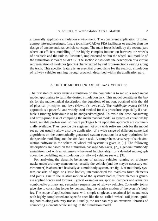
For analysing the dynamic behaviour of railway vehicles running on arbitrarytracks under arbitrary manoeuvres, usually the vehicle (and the maybe necessary en-vironment) is abstracted basically as a multibody system, see fig. 1. A multibody sys-tem consists of rigid or elastic bodies, interconnected via massless force elementsand joints. Due to the relative motion of the system’s bodies, force elements gener-ate applied forces and torques. Typical examples are springs, dampers and actuatorscombined to primary and secondary suspensions of railway vehicles. Contrarily, jointsgive rise to constraint forces by constraining the relative motion of the system’s bod-ies. The scope of applications starts with simple single axis rotational joints and endswith highly complicated and specific ones like the so–called ‘wheel–rail joints’ guid-ing bodies along arbitrary tracks. Usually, the user can rely on extensive libraries ofconnecting elements while setting up the simulation model.

3 MODELLING THE CONTACT BETWEEN WHEEL AND RAIL

t r a c k ( + i r r e g u l a r i t i e s )

C A D

F E Af r i c t i o n ,i m p a c t

f o r c e e l e m e n t sw i t h / w i t h o u t

d y n a m i c s

M B S

C A C E

M B S

C

w h e e l - r a i l i n t e r f a c e :c o n t a c t g e o m e t r yc o n t a c t f o r c e s

Figure 1. Generic simulation model for design and analysis of a railway vehicle’s running behaviour. (Pho-tograph: C. Splittberger, Internet:http://mercurio.iet.unipi.it.)

To serve the purpose of modern and future design criteria, bi–directional interfacesto well–known and established Computer Aided Engineering (CAE) software are re-quired additionally to reproduce specific phenomena. Thus, certain simulation tasksand requirements are easier to be performed – or become accomplishable at all, [4].

To take the flexibility of lightweight structures into account, an interface to dif-ferent Finite Element (FEA) software has been implemented. Here, in a first step, anumber of mode shapes of the body to be modelled elastically are calculated by FE–analysis. The results are then transferred to the multibody simulation, resulting in a‘hybrid’ model consisting of rigid and elastic bodies. Finally, on behalf of a dynamicstress analysis of the flexible body’s most endangered locations, the dynamic forcesand accelerations following from the time–integration of the system equations can beshifted back to the FE software, see also [5].

More and more electronically controlled elements like tilting systems etc. are im-plemented in vehicles to shorten overall travel times, to increase ride comfort andso on. One possibility to incorporate active/semi–active (i.e. feed back control) ele-ments into the simulation models of suchmechatronicsystems is to use internal con-troller design tools. For more advanced or more complex controller design tasks, a bi–directional interface to Computer Aided Control Engineering (CACE) software suchas MATLAB SIMULINK can be applied.

To incorporate physical and graphical Computer Aided Design (CAD) data, thusextending the graphical abilities of the software and concurrently making MBS setupfaster, easier and more secure, an interface to CAD software exists. Vice versa SIM -PACK can be used to support the design process within CAD software itself by dy-namic, quasi–static and kinematic analyses.


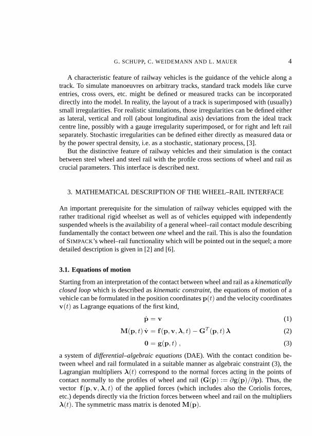
A characteristic feature of railway vehicles is the guidance of the vehicle along atrack. To simulate manoeuvres on arbitrary tracks, standard track models like curveentries, cross overs, etc. might be defined or measured tracks can be incorporateddirectly into the model. In reality, the layout of a track is superimposed with (usually)small irregularities. For realistic simulations, those irregularities can be defined eitheras lateral, vertical and roll (about longitudinal axis) deviations from the ideal trackcentre line, possibly with a gauge irregularity superimposed, or for right and left railseparately. Stochastic irregularities can be defined either directly as measured data orby the power spectral density, i.e. as a stochastic, stationary process, [3].

But the distinctive feature of railway vehicles and their simulation is the contactbetween steel wheel and steel rail with the profile cross sections of wheel and rail ascrucial parameters. This interface is described next.

3. MATHEMATICAL DESCRIPTION OF THE WHEEL–RAIL INTERFACE

An important prerequisite for the simulation of railway vehicles equipped with therather traditional rigid wheelset as well as of vehicles equipped with independentlysuspended wheels is the availability of a general wheel–rail contact module describingfundamentally the contact betweenonewheel and the rail. This is also the foundationof SIMPACK ’s wheel–rail functionality which will be pointed out in the sequel; a moredetailed description is given in [2] and [6].

3.1. Equations of motion

Starting from an interpretation of the contact between wheel and rail as akinematicallyclosed loopwhich is described askinematic constraint, the equations of motion of avehicle can be formulated in the position coordinatesp(t) and the velocity coordinatesv(t) as Lagrange equations of the first kind,

p = v (1)

M(p, t) v = f(p,v,λ, t)−GT (p, t) λ (2)

0 = g(p, t) , (3)

a system ofdifferential–algebraic equations(DAE). With the contact condition be-tween wheel and rail formulated in a suitable manner as algebraic constraint (3), theLagrangian multipliersλ(t) correspond to the normal forces acting in the points ofcontact normally to the profiles of wheel and rail (G(p) := ∂g(p)/∂p). Thus, thevector f(p,v,λ, t) of the applied forces (which includes also the Coriolis forces,etc.) depends directly via the friction forces between wheel and rail on the multipliersλ(t). The symmetric mass matrix is denotedM(p).


Replacing the constraint equations (3) by a stiff ‘Hertzian contact spring’, i.e. by aone–sided spring–damper force element, the equations of motion yield as a system ofordinary differential equations (ODE),y = fe(y, t), y := (pT ,vT )T . A typical appli-cation of this ‘elastic’ contact model would be the investigation of wheel–lift scenariosor derailments, but, particularly under a numerical point of view, the preceding ‘con-strained contact’ model ought to be preferred.

3.2. Contact geometry: A quasi–elastic contact model

Letd(s,q) be the distance between two corresponding points on the wheel and the railenvelope curves in vertical direction being parameterized by the lateral wheel profilecoordinates and the relative position vectorq of the wheel with respect to the rail.Since the position vectorq := q(p, t) depends on the MBS coordinatesp of eqs. (1)–(3), the classical contact condition

g(q) := minsd(s,q) = 0 (4)

also defines directly the kinematic constraint (3). The lateral coordinates of the con-tact point on the wheel follows then from the necessary condition

∂

∂sd(s,q)

∣∣∣s=s

= 0 . (5)

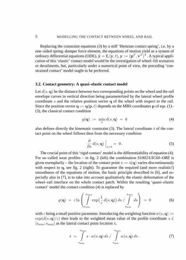
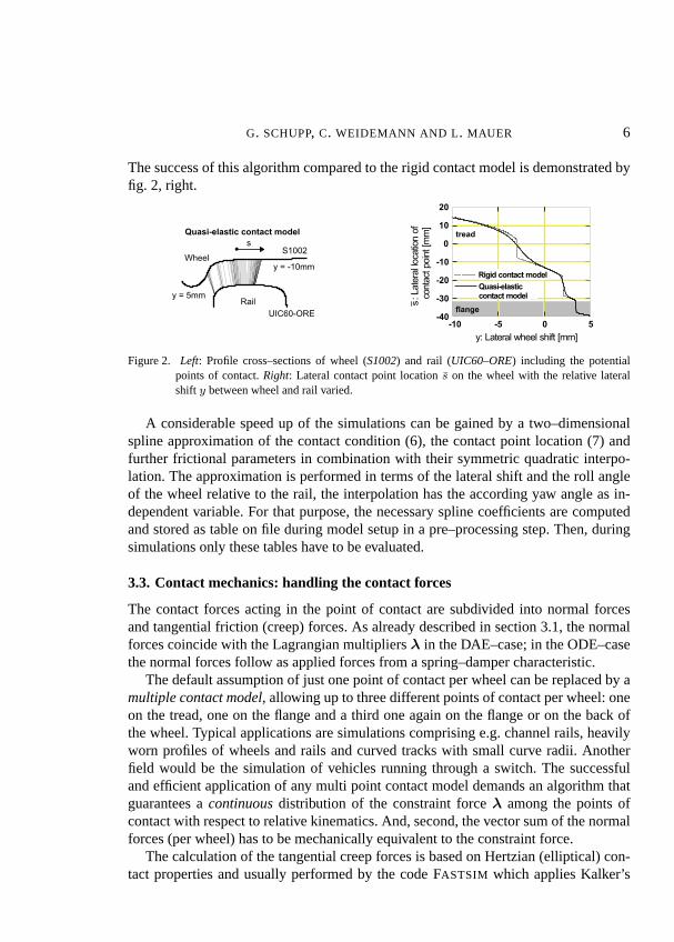
The crucial point of this ‘rigid contact’ model is the differentiability of equation (4).For so–called wear profiles – in fig. 2 (left) the combinationS1002/UIC60–OREisgiven exemplarily – the location of the contact points := s(q) varies discontinuouslywith respect toq, see fig. 2 (right). To guarantee the required (and more realistic!)smoothness of the equations of motion, the basic principle described in [6], and es-pecially also in [7], is to take into account qualitatively the elastic deformation of thewheel–rail interface on the whole contact patch. Within the resulting ‘quasi–elasticcontact’ model the contact condition (4) is replaced by

g(q) = ε ln

smax∫smin

exp(1εd(s,q)

)ds /

smax∫smin

ds

= 0 (6)

with ε being a small positive parameter. Introducing the weighting functionw(s,q) :=exp(d(s,q)/ε) then leads to the weighted mean value of the profile coordinates ∈[smin; smax] as the lateral contact point locations,

s =

smax∫smin

s · w(s,q) ds /

smax∫smin

w(s,q) ds . (7)


The success of this algorithm compared to the rigid contact model is demonstrated byfig. 2, right.

W h e e l

R a i l

S 1 0 0 2

U I C 6 0 - O R E

y = - 1 0 m m

y = 5 m m

Q u a s i - e l a s t i c c o n t a c t m o d e ls

t r e a d

f l a n g e

2 0

1 0

0

- 1 0

- 2 0

- 3 0

- 4 0- 1 0 - 5 0 5

y : L a t e r a l w h e e l s h i f t [ m m ]

R i g i d c o n t a c t m o d e l

Q u a s i - e l a s t i cc o n t a c t m o d e l: L

ater

al lo

catio

n of

cont

act p

oint

[mm

]s

Figure 2. Left: Profile cross–sections of wheel (S1002) and rail (UIC60–ORE) including the potentialpoints of contact.Right: Lateral contact point locations on the wheel with the relative lateralshift y between wheel and rail varied.

A considerable speed up of the simulations can be gained by a two–dimensionalspline approximation of the contact condition (6), the contact point location (7) andfurther frictional parameters in combination with their symmetric quadratic interpo-lation. The approximation is performed in terms of the lateral shift and the roll angleof the wheel relative to the rail, the interpolation has the according yaw angle as in-dependent variable. For that purpose, the necessary spline coefficients are computedand stored as table on file during model setup in a pre–processing step. Then, duringsimulations only these tables have to be evaluated.

3.3. Contact mechanics: handling the contact forces

The contact forces acting in the point of contact are subdivided into normal forcesand tangential friction (creep) forces. As already described in section 3.1, the normalforces coincide with the Lagrangian multipliersλ in the DAE–case; in the ODE–casethe normal forces follow as applied forces from a spring–damper characteristic.

The default assumption of just one point of contact per wheel can be replaced by amultiple contact model, allowing up to three different points of contact per wheel: oneon the tread, one on the flange and a third one again on the flange or on the back ofthe wheel. Typical applications are simulations comprising e.g. channel rails, heavilyworn profiles of wheels and rails and curved tracks with small curve radii. Anotherfield would be the simulation of vehicles running through a switch. The successfuland efficient application of any multi point contact model demands an algorithm thatguarantees acontinuousdistribution of the constraint forceλ among the points ofcontact with respect to relative kinematics. And, second, the vector sum of the normalforces (per wheel) has to be mechanically equivalent to the constraint force.

The calculation of the tangential creep forces is based on Hertzian (elliptical) con-tact properties and usually performed by the code FASTSIM which applies Kalker’s


simplified theory of rolling contact, [8]. Other friction laws, some of them with theadvantage of being analytically describable, are also in use, see e.g. [9]. Comparedto a computationally more expensive non–Hertzian contact description, the Hertziancontact model has the advantage that it can be characterized by four parameters (ra-tio of the semi axes of an equivalent contact ellipse and three normalized creepages).Therefore, using the quasi–elastic contact model, the main curvatures of wheel andrail defining the geometrical properties of the contact ellipse are obtained also by aweighted sum approach, analogously to the calculation of the contact point locationwith eq. (7).

3.4. Non–constant rail profiles

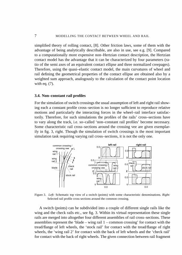
For the simulation of switch crossings the usual assumption of left and right rail show-ing each a constant profile cross–section is no longer sufficient to reproduce relativemotions and particularly the interacting forces in the wheel–rail interface satisfac-torily. Therefore, for such simulations the profiles of the rails’ cross–sections haveto vary along the track, i.e. so–called ‘non–constant rail profiles’ become necessary.Some characteristic rail cross–sections around the crossing vee are given exemplar-ily in fig. 3, right. Though the simulation of switch crossings is the most importantsimulation task requiring varying rail cross–sections, it is not the only one.

123

w i n gr a i l 1

w i n gr a i l 2

s t o c k r a i l

c o m m o n c r o s s i n g /c r o s s i n g v e e

c h e c k r a i lb l a d e

L

1

2

3

0 . 0

0 . 0

0 . 0

0 . 0

0 . 0

0 . 0

0 . 00 . 0

l e f t r a i l r i g h t r a i l

1

2

3

c o m m o n c r o s s i n g /c r o s s i n g v e e s t o c k r a i l

c h e c k r a i lw i n g

r a i l 2

w i n gr a i l 1

Figure 3. Left: Schematic top view of a switch (points) with some characteristic denominations.Right:Selected rail profile cross sections around the common crossing.

A switch (points) can be subdivided into a couple of different single rails like thewing and the check rails etc., see fig. 3. Within its virtual representation these singlerails are merged into altogether four different assemblies of rail cross–sections. Theseassemblies represent the ‘blade – wing rail 1 – common crossing’ for contact with thetread/flange of left wheels, the ‘stock rail’ for contact with the tread/flange of rightwheels, the ‘wing rail 2’ for contact with the back of left wheels and the ‘check rail’for contact with the back of right wheels. The given connection between rail fragment


and wheel part is valid only for the crossing scenario shown in fig. 3, left, i.e. if thevehicle follows the route turning out on the right hand side of the straight track.

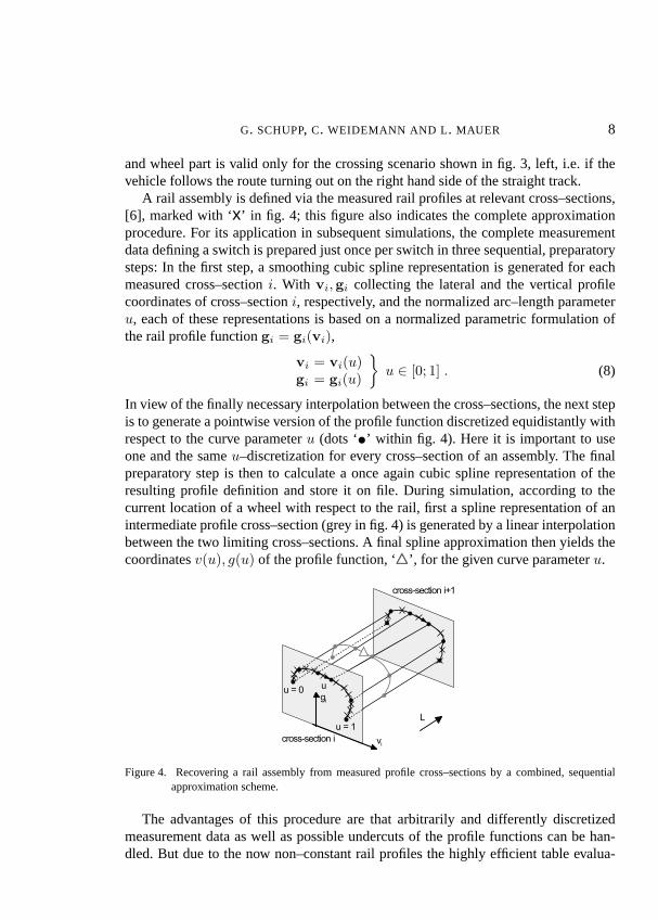
A rail assembly is defined via the measured rail profiles at relevant cross–sections,[6], marked with ‘x’ in fig. 4; this figure also indicates the complete approximationprocedure. For its application in subsequent simulations, the complete measurementdata defining a switch is prepared just once per switch in three sequential, preparatorysteps: In the first step, a smoothing cubic spline representation is generated for eachmeasured cross–sectioni. With vi,gi collecting the lateral and the vertical profilecoordinates of cross–sectioni, respectively, and the normalized arc–length parameteru, each of these representations is based on a normalized parametric formulation ofthe rail profile functiongi = gi(vi),

vi = vi(u)gi = gi(u)

}u ∈ [0; 1] . (8)

In view of the finally necessary interpolation between the cross–sections, the next stepis to generate a pointwise version of the profile function discretized equidistantly withrespect to the curve parameteru (dots ‘•’ within fig. 4). Here it is important to useone and the sameu–discretization for every cross–section of an assembly. The finalpreparatory step is then to calculate a once again cubic spline representation of theresulting profile definition and store it on file. During simulation, according to thecurrent location of a wheel with respect to the rail, first a spline representation of anintermediate profile cross–section (grey in fig. 4) is generated by a linear interpolationbetween the two limiting cross–sections. A final spline approximation then yields thecoordinatesv(u), g(u) of the profile function, ‘444’, for the given curve parameteru.

c r o s s - s e c t i o n i

c r o s s - s e c t i o n i + 1

v i

g i

u = 0

u = 1

u

L

Figure 4. Recovering a rail assembly from measured profile cross–sections by a combined, sequentialapproximation scheme.

The advantages of this procedure are that arbitrarily and differently discretizedmeasurement data as well as possible undercuts of the profile functions can be han-dled. But due to the now non–constant rail profiles the highly efficient table evalua-


tions of the contact geometry and parameters described at the end of section 3.2 haveto be replaced by the online mode of their calculation.

4. APPLICATION EXAMPLE: A RAILWAY VEHICLERUNNING THROUGH A SWITCH

4.1. Areas of Application

The simulation of a railway vehicle travelling through a switch is to some degree asophisticated task, as can be seen from the above explanations. In contrast, there aremany potential cases of application that are worth examining. In general, the forcesacting between wheel and rail are considerably higher in switches and crossings thanon standard track. Because of their high dynamics resulting from the rapidly changingrail profile forms they may have a worse influence on the passenger ride comfort andthe lifetime of bogie components than narrow curves or track irregularities. For allthat, up to now only few realistic data are available about the wheel/rail forces actingwithin switches and crossings. Hence, such simulations are useful e.g.r for determining the wheel/rail forces (lateral,Y , and vertical,Q) and their high

dynamics within the switch,r for the generation of load collectives for a series of switches and/or crossings andthe corresponding vehicles in a railway system orr for minimising the load on wheels and rails as well as improving the passenger ridecomfort by optimising the profile geometry of the switch.

Another promising application of switch simulation can be the examination of theguidance behaviour or the space that the wheels will require in the switch. Switchesare known to have some crucial points that are susceptible to derailments or intensewear: the beginning of the blade rail, especially in the divergent route, or the area nearthe crossing vee, where the wheelset will be guided by the check rail. In these casesonly the simulation is able to predict reliably the position of the wheels in the gaugechannel and their addiction to derailment.

4.2. Unusual modelling features

Even if ‘non–constant rail profiles’ as described in section 3.4 are the most importantmodelling feature for simulations of railway vehicles running through a switch, a cou-ple of extraordinary modelling elements have to be provided additionally to reproducethe unusual contact situations between wheels and rails that have to be anticipated inthis case, [6]. Those situations occur e.g. if one wheel is in the vicinity of the crossingvee, see fig. 3; the following descriptions refer to the crossing scenario given there.


The wheel running over the crossing vee has to change its contact from the bladerail to the through rail (or vice versa), which leads usually to more than one point ofcontact per wheel – at least one on its tread and one on its flange has to be expected.How this multiple contact situation can be handled has been outlined in section 3.3.

Also around the crossing vee, a wheel can loose its contact with the rail. This wheellift, indicated by a vanishing constraint forceλ = 0, means a structural change of theequations of motion because the constraint or contact condition (6) is no longer valid.Once wheel lift is detected during simulation by means of a root function technique,the constraint between wheel and rail is replaced automatically by the ‘elastic’ contactmodel utilizing a one–sided spring–damper element as described in section 3.1.

As long as the wheel runs in the vicinity of the crossing vee, the wheelset is guidedby the contact of the opposite wheel’s back with the check rail, while the back ofthe wheel on the crossing vee may contact wing rail 2. Hence, an additional contactelement between the back of each wheel and the check/wing rails is necessary. Sincethose contacts are usually rather short–time, again the ‘elastic’ contact formulation ischosen for this case.

4.3. The simulation model

The vehicle used for the examination is a standard passenger car running on Vignol railprofiles, modelled with the multibody simulation package SIMPACK based on the dataof the ‘Manchester Benchmark’ [1, 10]. Its overall data can be found in table 1. Themodel uses standard elements for primary and secondary suspension, that are equippedwith linear spring and damper characteristics. For the wheel/rail contact SIMPACK ’smulti contact model is chosen in order to reproduce the special contact situations atthe beginning of the blade rail and on the crossing vee. With this method, up to threedifferent contact points on each wheel are possible. Furthermore, for the guard railcontact also the back-of-wheel contact is active.

A standard switch of type ‘EW 60-300-1:9’ is used for the examination, which canbe found e. g. on feeder lines or in stations in Germany. Its overall data are shown intable 1 as well.

The profile cross sections needed for the modelling of the non–constant rail pro-files are taken from a three–dimensional CAD model set up previously according tothe technical drawings of the switch [11]. This is necessary because the technicaldrawings themselves do not depict all the cross sections needed in the simulation. Onthe contrary, some parts of the changing rail profiles are only given by an explanationof the manufacturing process, e. g. by depicting the tool and its movement when plan-ing the raw rail. Instead of converting the profile coordinates from a CAD model, alsomeasured profile data could be used.

The switch model consists of 55 different cross sections that are used in total 83–times at the appropriate positions in the switch. The high number of cross sections is


Table 1. Overall data of the passenger vehicle and the switch.

Total mass 45800 kgTotal length 26.4 mBogie distance 19 mWheelset distance 2.56 mNr. of wheelsets 4, in 2 bogiesTrack gauge 1435 mmWheel profile S 1002Switch denotation EW 60-300-1:9Stock rail profile UIC 60, not cantedTravelled route divergent route, left-handSwitch angle 6.37◦ (1:9)Radius of divergent route 300 m, no curve entry/exitGuard rail denotation Rl 1–60

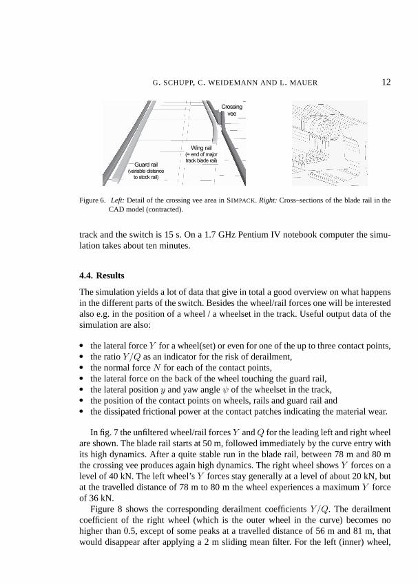
necessary in order to ensure a correct profile interpolation even between very unalikeprofile forms. Figure 6 (right) shows the cross–sections used for the blade rail.

Because of the high forces in the crucial regions of the switch and their high dy-namics it is necessary to work with an elastic track model. Here a standard trackrepresentation is used, consisting of one equivalent mass per wheelset that representsthe ballast and the sleeper. It is suspended with respect to the inertia system by meansof spring/damper elements. The mass and the (here constant) spring and damper coef-ficients are taken from [12].

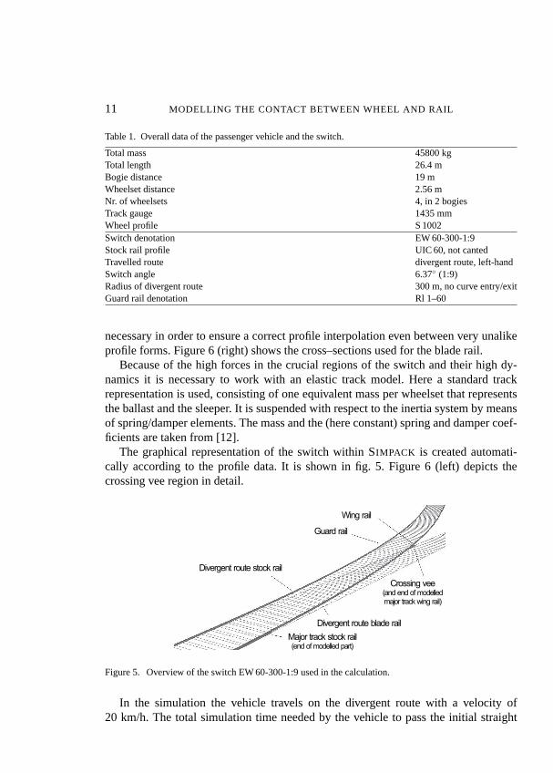
The graphical representation of the switch within SIMPACK is created automati-cally according to the profile data. It is shown in fig. 5. Figure 6 (left) depicts thecrossing vee region in detail.

D i v e r g e n t r o u t e s t o c k r a i l

M a j o r t r a c k s t o c k r a i l( e n d o f m o d e l l e d p a r t )

D i v e r g e n t r o u t e b l a d e r a i l

G u a r d r a i l

W i n g r a i l

C r o s s i n g v e e( a n d e n d o f m o d e l l e dm a j o r t r a c k w i n g r a i l )

Figure 5. Overview of the switch EW 60-300-1:9 used in the calculation.

In the simulation the vehicle travels on the divergent route with a velocity of20 km/h. The total simulation time needed by the vehicle to pass the initial straight


G u a r d r a i l( v a r i a b l e d i s t a n c e

t o s t o c k r a i l )

W i n g r a i l( = e n d o f m a j o rt r a c k b l a d e r a i l )

C r o s s i n gv e e

Figure 6. Left: Detail of the crossing vee area in SIMPACK. Right: Cross–sections of the blade rail in theCAD model (contracted).

track and the switch is 15 s. On a 1.7 GHz Pentium IV notebook computer the simu-lation takes about ten minutes.

4.4. Results

The simulation yields a lot of data that give in total a good overview on what happensin the different parts of the switch. Besides the wheel/rail forces one will be interestedalso e.g. in the position of a wheel / a wheelset in the track. Useful output data of thesimulation are also:r the lateral forceY for a wheel(set) or even for one of the up to three contact points,r the ratioY/Q as an indicator for the risk of derailment,r the normal forceN for each of the contact points,r the lateral force on the back of the wheel touching the guard rail,r the lateral positiony and yaw angleψ of the wheelset in the track,r the position of the contact points on wheels, rails and guard rail andr the dissipated frictional power at the contact patches indicating the material wear.

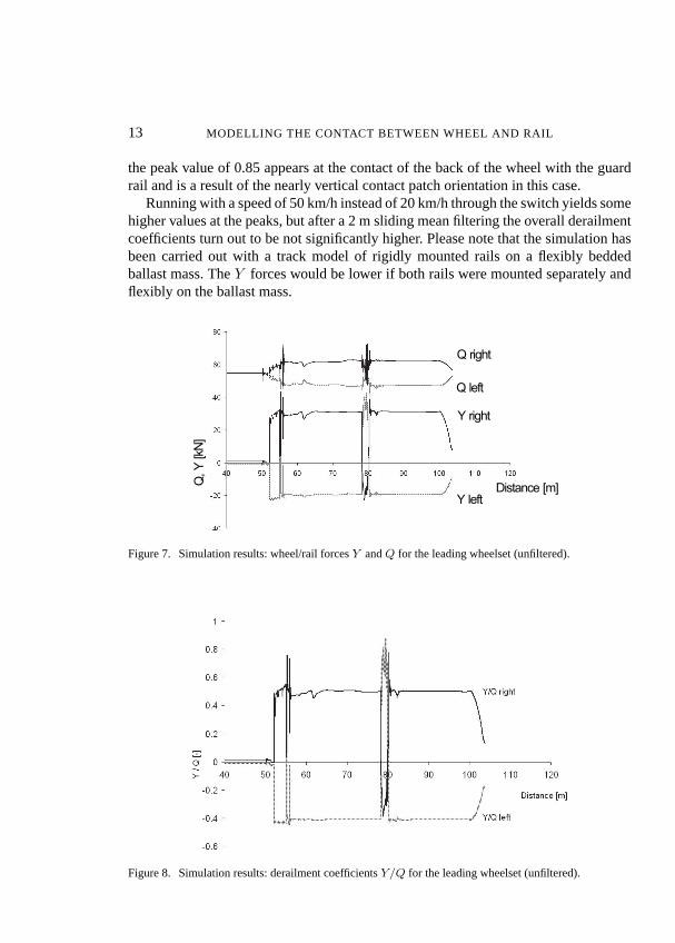
In fig. 7 the unfiltered wheel/rail forcesY andQ for the leading left and right wheelare shown. The blade rail starts at 50 m, followed immediately by the curve entry withits high dynamics. After a quite stable run in the blade rail, between 78 m and 80 mthe crossing vee produces again high dynamics. The right wheel showsY forces on alevel of 40 kN. The left wheel’sY forces stay generally at a level of about 20 kN, butat the travelled distance of 78 m to 80 m the wheel experiences a maximumY forceof 36 kN.

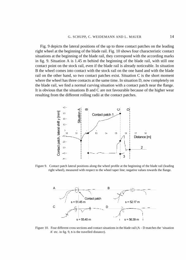
Figure 8 shows the corresponding derailment coefficientsY/Q. The derailmentcoefficient of the right wheel (which is the outer wheel in the curve) becomes nohigher than 0.5, except of some peaks at a travelled distance of 56 m and 81 m, thatwould disappear after applying a 2 m sliding mean filter. For the left (inner) wheel,


the peak value of 0.85 appears at the contact of the back of the wheel with the guardrail and is a result of the nearly vertical contact patch orientation in this case.

Running with a speed of 50 km/h instead of 20 km/h through the switch yields somehigher values at the peaks, but after a 2 m sliding mean filtering the overall derailmentcoefficients turn out to be not significantly higher. Please note that the simulation hasbeen carried out with a track model of rigidly mounted rails on a flexibly beddedballast mass. TheY forces would be lower if both rails were mounted separately andflexibly on the ballast mass.

D i s t a n c e [ m ]

Y r i g h t

Q r i g h t

Q l e f t

Y l e f t

Q, Y

[kN

]

Figure 7. Simulation results: wheel/rail forcesY andQ for the leading wheelset (unfiltered).

Figure 8. Simulation results: derailment coefficientsY/Q for the leading wheelset (unfiltered).


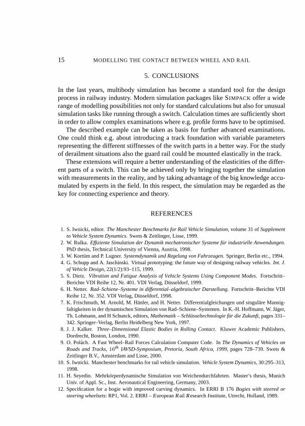
Fig. 9 depicts the lateral positions of the up to three contact patches on the leadingright wheel at the beginning of the blade rail. Fig. 10 shows four characteristic contactsituations at the beginning of the blade rail, they correspond with the according marksin fig. 9. Situation A is 1.45 m behind the beginning of the blade rail, with still onecontact point on the stock rail, even if the blade rail is already noticeable. In situationB the wheel comes into contact with the stock rail on the one hand and with the bladerail on the other hand, so two contact patches exist. Situation C is the short momentwhere the wheel has three contacts at the same time. In situation D, now completely onthe blade rail, we find a normal curving situation with a contact patch near the flange.It is obvious that the situations B and C are not favourable because of the higher wearresulting from the different rolling radii at the contact patches.

Con

tact

pat

ch, l

ater

al s

hift

y [m

m]

Situ

atio

n A B C D

D i s t a n c e [ m ]

C o n t a c t p a t c h 1

2

3

Figure 9. Contact patch lateral positions along the wheel profile at the beginning of the blade rail (leadingright wheel), measured with respect to the wheel taper line; negative values towards the flange.

s = 5 2 . 1 7 m

s = 5 5 . 4 0 m s = 5 6 . 3 9 m

s = 5 1 . 4 5 m

A B

DC

C o n t a c t p a t c h

Figure 10. Four different cross sections and contact situations in the blade rail (A – D matches the ‘situationA’ etc. in fig. 9,s is the travelled distance).


5. CONCLUSIONS

In the last years, multibody simulation has become a standard tool for the designprocess in railway industry. Modern simulation packages like SIMPACK offer a widerange of modelling possibilities not only for standard calculations but also for unusualsimulation tasks like running through a switch. Calculation times are sufficiently shortin order to allow complex examinations where e.g. profile forms have to be optimised.

The described example can be taken as basis for further advanced examinations.One could think e.g. about introducing a track foundation with variable parametersrepresenting the different stiffnesses of the switch parts in a better way. For the studyof derailment situations also the guard rail could be mounted elastically in the track.

These extensions will require a better understanding of the elasticities of the differ-ent parts of a switch. This can be achieved only by bringing together the simulationwith measurements in the reality, and by taking advantage of the big knowledge accu-mulated by experts in the field. In this respect, the simulation may be regarded as thekey for connecting experience and theory.

REFERENCES

1. S. Iwnicki, editor.The Manchester Benchmarks for Rail Vehicle Simulation, volume 31 ofSupplementto Vehicle System Dynamics. Swets & Zeitlinger, Lisse, 1999.

2. W. Rulka. Effiziente Simulation der Dynamik mechatronischer Systeme fur industrielle Anwendungen.PhD thesis, Technical University of Vienna, Austria, 1998.

3. W. Kortum and P. Lugner.Systemdynamik und Regelung von Fahrzeugen. Springer, Berlin etc., 1994.4. G. Schupp and A. Jaschinski. Virtual prototyping: the future way of designing railway vehicles.Int. J.

of Vehicle Design, 22(1/2):93–115, 1999.5. S. Dietz. Vibration and Fatigue Analysis of Vehicle Systems Using Component Modes. Fortschritt–

Berichte VDI Reihe 12, Nr. 401. VDI Verlag, Dusseldorf, 1999.6. H. Netter. Rad–Schiene–Systeme in differential–algebraischer Darstellung. Fortschritt–Berichte VDI

Reihe 12, Nr. 352. VDI Verlag, Dusseldorf, 1998.7. K. Frischmuth, M. Arnold, M. Hanler, and H. Netter. Differentialgleichungen und singulare Mannig-

faltigkeiten in der dynamischen Simulation von Rad–Schiene–Systemen. In K.-H. Hoffmann, W. Jager,Th. Lohmann, and H Schunck, editors,Mathematik – Schlusseltechnologie fur die Zukunft, pages 331–342. Springer–Verlag, Berlin Heidelberg New York, 1997.

8. J. J. Kalker. Three–Dimensional Elastic Bodies in Rolling Contact. Kluwer Academic Publishers,Dordrecht, Boston, London, 1990.

9. O. Polach. A Fast Wheel–Rail Forces Calculation Computer Code. InThe Dynamics of Vehicles onRoads and Tracks,16th IAVSD-Symposium, Pretoria, South Africa, 1999, pages 728–739. Swets &Zeitlinger B.V., Amsterdam and Lisse, 2000.

10. S. Iwnicki. Manchester benchmarks for rail vehicle simulation.Vehicle System Dynamics, 30:295–313,1998.

11. H. Seyedin. Mehrkorperdynamische Simulation von Weichendurchfahrten. Master’s thesis, MunichUniv. of Appl. Sc., Inst. Aeronautical Engineering, Germany, 2003.

12. Specification for a bogie with improved curving dynamics. In ERRI B 176Bogies with steered orsteering wheelsets: RP1, Vol. 2. ERRI –EuropeanRail ResearchInstitute, Utrecht, Holland, 1989.

Documents

Modelling the Contact between Wheel and Rail within ... · Modelling the Contact between Wheel and Rail within Multibody System Simulation GUNTER SCHUPP1, ... design method during