ENOC-2008, Saint Petersburg, Russia, June 30–July 4 2008

MODELLING THE DYNAMICS OF A RIGID ROTOR IN ACTIVE MAGNETIC BEARINGS

Gennadii Martynenko Faculty of Engineering Physics, Department of Dynamics and Strength of Machines

National Technical University Kharkiv Polytechnic Institute Ukraine

gmartynenko@kpi.kharkov.ua

Abstract The paper deals with developing a mathematical

model of a rigid rotor in active radial and axial elec-tromagnetic bearings. A feature of the suggested technique of mathemati-

cal description of rotor dynamic behaviour is ac-counting for the nonlinear relationship of mechani-cal and electromagnetic processes in the system. The magnetic conductance of gaps under the poles of the electromagnets is defined with account of the mutual impact of radial and axial rotor displace-ment. The analytical model described can be used as a

basis of the simulation computer model for alterna-tive dynamic stability calculations to select effective suspension parameters and control actions for dif-ferent design options.

Key words Dynamics of rotor systems, active magnetic bear-

ings, mathematical model

1 Introduction Active magnetic bearings (AMB) are an alternative

to frictionless, sliding and gas-dynamic bearings, and, as compared to these, have several advantages (no lubrication systems, reduced friction loss, com-paratively big gap, and others) [Siegwart, Bleuler and Traxler, 2000]. During a mathematical description of a rotor-

AMB system, the following parts are distinguished: the rotor mathematical model, the bearing model and the control law effected by the control system [Steven, Nataraj, 2007]. Correct definition and validation of control algo-

rithm parameters with numerical experiments is possible only with adequate mathematical modelling of the rotor-AMB system and interrelated magnetic and mechanical phenomena occuring therein. In analysing several technical devices, the electro-

mechanical vibration equations are linearised. Such an approach was also used for AMB [Schweitzer, Bleuler and Traxler, 1994]. Thus, the magneto-

mechanical rotor in AMB system is modelled with motion differential equations and differential equa-tions for currents in the linear approximation. In so doing, the currents in the circuits and the control voltages in the windings are linearised about the equilibrium position [Maslen, 2000]. The suspension linear model is written down on

the assumption of smallness of deviations of vari-ables from their rated values. Actually, these devia-tions can be significant. Hence, in limit conditions – magnetic circuit saturation, zero current, zero gap, and so forth – the linear suspension model becomes meaningless [Zhuravlyov, 2003]. Thus, with circuit currents close to zero, linearisation about the equi-librium position is incorrect. When rotor displace-ments are comparable with the rated gap, the mathematical model is also incorrect. These deficiencies can also be inherent to rotor po-

sition control units built around such linearised models. This paper considers a nonlinear mathematical

model of a rigid rotor in AMB. The model accounts for the relation between axial and radial rotor dis-placements when defining the magnetic conduc-tances of gaps under the poles of magnetic bearings. The fluxes in the AMB magnetic circuits have been defined using detail equivalent circuits with account of magnetic resistances of air gaps under the poles and between them, as well as in stator and rotor sec-tions. In the paper, one of the possible designs of a com-

plete electromagnetic rotor suspension with two 8-pole radial bearings and one axial bearing with an armature in the form of a pot core has been mod-elled.

2 Description of electromechanical systems Technical electromechanical systems are described

by Lagrange-Maxwell equations structured as me-chanics equations. When conductance currents are closed and there are no capacitors in the electric paths, electromechanical systems are described by equations similar to Routh equations in mechanics

[Hodzhaev, 1979]:

⎪⎭

⎪⎬⎫

==∑+

=+−=+−

=Ψ∂∂

∂Ψ∂

∂∂

∂∂

∂∂

∂∂

∂∂

),...,1(

),...,1(

1

Π

NkEr

MrQ

kN

s sW

ksCtk

rrqW

rqrqT

rqT

t & (1)

where Т is kinetic energy; П is potential energy; W=W(Ψ1,…, ΨN, q1,…, qM) is magnetic field en-ergy; qr are generalised mechanical coordinates; Qr are nonpotential generalised forces; M is the number of generalised mechanical coordinates; Ψk are in-duction fluxes (flux linkages); N is the number of closed nonbranching loops with loop currents ik; rCks are active resistances of electric circuits, and Ek is algebraic sum of external electromotive forces in the k-th loop, and

sW

skiW

k i Ψ∂∂

∂∂ ==Ψ , . (2)

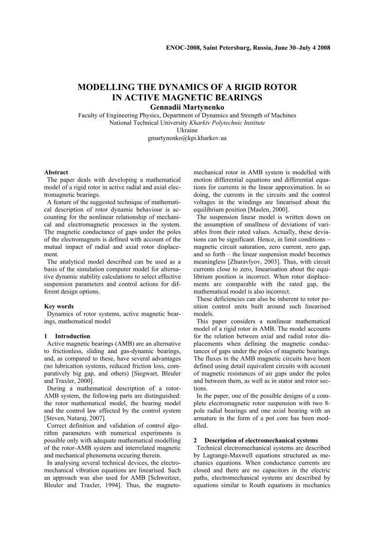
3 Rotor magnetic suspension layout In the paper, the technique of mathematical de-

scription of the rotor-AMB system is considered by example of one of the possible alternatives of the model of the complete electromagnetic rotor sus-pension shown in Figure 1.

Figure 1. Model and layout of a complete electromagnetic rotor

suspension.

Typical 8-pole magnetic bearings are used as two radial ones (Fig. 2), and a typical thrust magnetic bearing with pot cores is used as the axial one (Fig. 3) [Maslen, 2000].

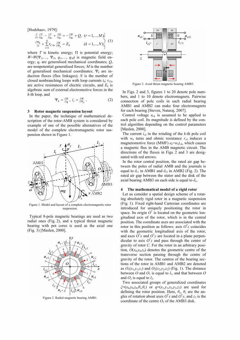
Figure 2. Radial magnetic bearing AMB1.

Figure 3. Axial thrust magnetic bearing AMB3.

In Figs. 2 and 3, figures 1 to 20 denote pole num-

bers, and 1 to 10 denote electromagnets. Pairwise connection of pole coils in each radial bearing AMB1 and AMB2 can make four electromagnets for each bearing [Steven, Nataraj, 2007]. Control voltage uck is assumed to be applied to

each pole coil. Its magnitude is defined by the con-trol algorithm depending on the control parameters [Maslen, 2000]. The current ick in the winding of the k-th pole coil

with wk turns and ohmic resistance rck induces a magnetomotive force (MMF) ek=wkick, which causes a magnetic flux in the AMB magnetic circuit. The directions of the fluxes in Figs. 2 and 3 are desig-nated with red arrows. In the rotor central position, the rated air gap be-

tween the poles of radial AMB and the journals is equal to δr1 in AMB1 and δr2 in AMB2 (Fig. 2). The rated air gap between the stator and the disk of the axial bearing AMB3 on each side is equal to δa. 4 The mathematical model of a rigid rotor Let us consider a spatial design scheme of a rotat-

ing absolutely rigid rotor in a magnetic suspension (Fig. 1). Fixed right-hand Cartesian coordinates are introduced for uniquely positioning the rotor in space. Its origin O* is located on the geometric lon-gitudinal axis of the rotor, which is in the central position. The coordinate axes are associated with the rotor in this position as follows: axis O*z coincides with the geometric longitudinal axis of the rotor, and axes O*x and O*y are located in a plane perpen-dicular to axis O*z and pass through the centre of gravity of rotor C. For the rotor in an arbitrary posi-tion, O(x0,y0,z0) denotes the geometric centre of the transverse section passing through the centre of gravity of the rotor. The centres of the bearing sec-tions of the rotor in AMB1 and AMB2 are denoted as O1(x1,y1,z1) and O2(x2,y2,z2) (Fig. 1). The distance between O and O1 is equal to l1, and that between O and O2 is equal to l2. Two associated groups of generalized coordinates ξ=(x0,y0,z0,θx,θy) or q=(x1,y1,x2,y2,z3) are used for defining the rotor position. Here, θx, θy are the an-gles of rotation about axes O*x and O*y, and z3 is the coordinate of the centre O3 of the AMB3 disk.

The mechanical part of the mathematical model of a rotating absolutely rigid rotor in AMB, with the number of generalized mechanical coordinates M=5 according to (1), is described by a system of differ-ential equations [Poznjak, 1980]:

⎪⎪⎪⎪⎪⎪⎪

⎭

⎪⎪⎪⎪⎪⎪⎪

⎬

⎫

+−+

+−=−

−−+

+−=+

−=

++−=

−+−=

∂∂

∂∂

∂∂

∂∂

∂∂

).cossin()(

);sincos()(

;

);cossin(

);sincos(

212

2

221

2

2

202

02

212

020

221

202

02

ttJJ

QJJ

ttJJ

QJJ

Qm

ttmQm

ttmQm

pe

yW

ydtxd

pdt

yde

pe

xW

xdtyd

pdtxd

e

zW

zdt

zd

yW

ydt

yd

xW

xdt

xd

ωγωγω

ω

ωγωγω

ω

ωεωεω

ωεωεω

θθθθ

θθθθ (3)

where m is rotor mass; e1, e2 and γ1, γ2 are linear and angular nonequilibrium parameters; Je, Jp are rotor equatorial and polar moments of inertia; ω is angu-lar velocity; Pξr=-∂W/∂ξr are suspension electro-magnetic responses, and Q are generalized external forces and moments.

5 Model of magnetic bearings To consider the option of a complete electromag-

netic suspension (Fig. 1), an AMB contains N=18 electromagnetic circuits with currents ick, ohmic resistances rck and input voltages uck (control sig-nals). Saturation and magnetic hysteresis is ignored. Then the electromagnetic part of the mathematical model according to (1) includes N=18 differential equations with respect to flux linkages. These equa-tions correspond to Kirchhoff's second law for mag-netic circuits and are a form of notation of the net current law for each k-th circuit: ),...,1( Nkur ckck

Wckt

ck ==+ Ψ∂∂

∂Ψ∂ , (4)

where Ψck is flux linkage (net magnetic fluxes through the coil circuits). If we assume that the magnetic flux conducted by

each coil turn is the same, then the total or net mag-netic flux through the coil loop will be kkkc w Φ=Ψ . (5) The magnetic flux Φk through area Sk of a magnetic

circuit section is equal to [Bessonov, 1973] kkk SB=Φ . (6) The magnetic resistance of a magnetic circuit sec-

tion [Bessonov, 1973] is

kSkkl

kR µµ0= , (7)

where lk is length of a magnetic circuit section; Sk is cross-section area; µ0 is permeability of vacuum; µk is relative magnetic permeability of the circuit sec-tion material. Then the energy of the magnetic field of the circuit

section [Bessonov, 1973] is equal to

221

kkk RW Φ= , (8) and the energy of the entire magnetic circuit is equal to the sum of energies of this circuit sections. If WI, WII and WIII denote the energy of AMB1,

AMB2 and AMB3 circuits, respectively, then the energy of the magnetic field in the magnetic circuits of a complete electromagnetic rotor suspension in AMB is equal to: IIIIII WWWW ++= . (9)

5.1 Determining magnetic fluxes The net flux linkage of the k-th loop Ψck is a func-

tion of both the current in the k-th loop and the cur-rents in other loops magnetically linked with the k-th loop [Bessonov, 1973]. In this case, detail equiva-lent circuits are suggested to be used for correct determination of magnetic fluxes in magnetic circuit sections. The magnetic fluxes in the magnetic circuit of the

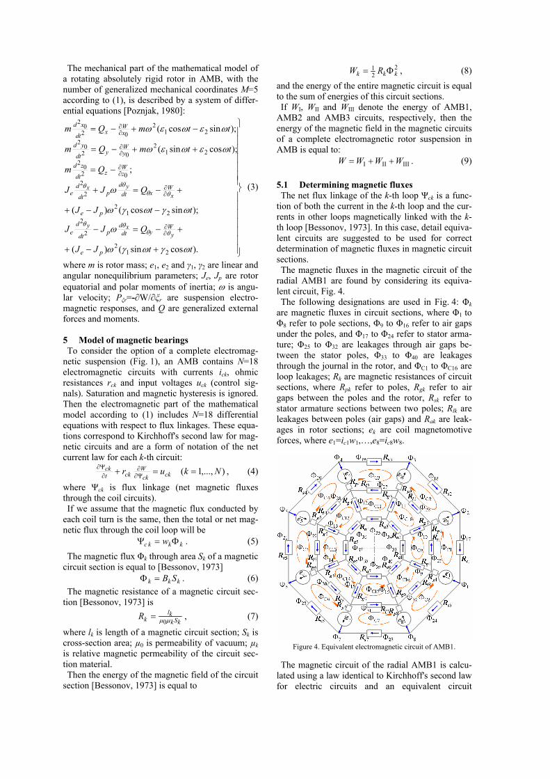
radial AMB1 are found by considering its equiva-lent circuit, Fig. 4. The following designations are used in Fig. 4: Φk

are magnetic fluxes in circuit sections, where Φ1 to Φ8 refer to pole sections, Φ9 to Φ16 refer to air gaps under the poles, and Φ17 to Φ24 refer to stator arma-ture; Φ25 to Φ32 are leakages through air gaps be-tween the stator poles, Φ33 to Φ40 are leakages through the journal in the rotor, and ΦС1 to ΦС16 are loop leakages; Rk are magnetic resistances of circuit sections, where Rpk refer to poles, Rgk refer to air gaps between the poles and the rotor, Rsk refer to stator armature sections between two poles; Rlk are leakages between poles (air gaps) and Rak are leak-ages in rotor sections; ek are coil magnetomotive forces, where e1=ic1w1,…,e8=ic8w8.

Figure 4. Equivalent electromagnetic circuit of AMB1.

The magnetic circuit of the radial AMB1 is calcu-

lated using a law identical to Kirchhoff's second law for electric circuits and an equivalent circuit

(Fig. 4). Magnetic circuits are calculated using dif-ferent methods, including the node-potential or the loop flux ones. Using the loop flux method (an ana-log of the loop current method) yields a system of algebraic equations with respect to loop fluxes. Its solution allows finding loop fluxes used for deter-mining the fluxes in all paths. Thus the fluxes in non-adjacent paths are equal to loop fluxes if their directions coincide, and are equal to loop fluxes with a reverse sign if they do not coincide. The fluxes in non-adjacent paths are also defined [Bo-risov, Lipatov, Zorin, 1985]. The magnetic fluxes Φ41 to Φ80 in the magnetic cir-

cuit of the radial AMB2 were determined using the same approach based on considering similar models and equivalent circuits (Figs. 2 and 4). The magnetic circuit of the axial AMB3 were re-

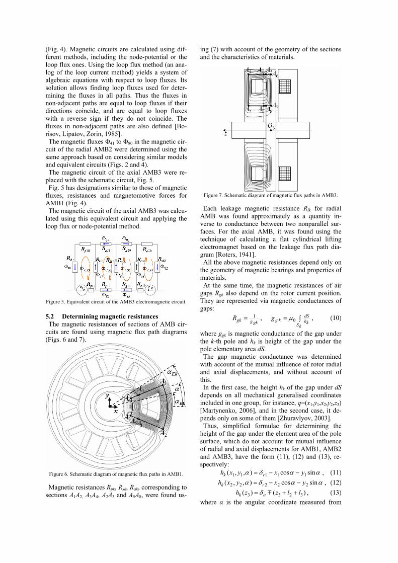
placed with the schematic circuit, Fig. 5. Fig. 5 has designations similar to those of magnetic

fluxes, resistances and magnetomotive forces for AMB1 (Fig. 4). The magnetic circuit of the axial AMB3 was calcu-

lated using this equivalent circuit and applying the loop flux or node-potential method.

Figure 5. Equivalent circuit of the AMB3 electromagnetic circuit.

5.2 Determining magnetic resistances The magnetic resistances of sections of AMB cir-

cuits are found using magnetic flux path diagrams (Figs. 6 and 7).

Figure 6. Schematic diagram of magnetic flux paths in AMB1.

Magnetic resistances Rpk, Rsk, Rak, corresponding to

sections A1A2, A3A4, A2A3 and A5A8, were found us-

ing (7) with account of the geometry of the sections and the characteristics of materials.

Figure 7. Schematic diagram of magnetic flux paths in AMB3.

Each leakage magnetic resistance Rlk for radial

AMB was found approximately as a quantity in-verse to conductance between two nonparallel sur-faces. For the axial AMB, it was found using the technique of calculating a flat cylindrical lifting electromagnet based on the leakage flux path dia-gram [Roters, 1941]. All the above magnetic resistances depend only on

the geometry of magnetic bearings and properties of materials. At the same time, the magnetic resistances of air

gaps Rgk also depend on the rotor current position. They are represented via magnetic conductances of gaps: ∫==

kS khdS

kggkggk gR 01 , µ , (10)

where ggk is magnetic conductance of the gap under the k-th pole and hk is height of the gap under the pole elementary area dS. The gap magnetic conductance was determined

with account of the mutual influence of rotor radial and axial displacements, and without account of this. In the first case, the height hk of the gap under dS

depends on all mechanical generalised coordinates included in one group, for instance, q=(x1,y1,x2,y2,z3) [Martynenko, 2006], and in the second case, it de-pends only on some of them [Zhuravlyov, 2003]. Thus, simplified formulae for determining the

height of the gap under the element area of the pole surface, which do not account for mutual influence of radial and axial displacements for AMB1, AMB2 and AMB3, have the form (11), (12) and (13), re-spectively: ααδα sincos),,( 11111 yxyxh rk −−= , (11) ααδα sincos),,( 22222 yxyxh rk −−= , (12) )()( 3233 llzzh ak ++= mδ , (13) where α is the angular coordinate measured from

axis O*x, which changes within the angular coordi-nates of the beginning (αBk) and end (αEk) of the k-th pole of the radial AMB.

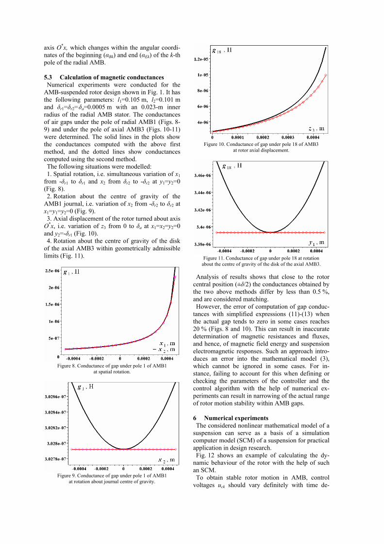
5.3 Calculation of magnetic conductances Numerical experiments were conducted for the

AMB-suspended rotor design shown in Fig. 1. It has the following parameters: l1=0.105 m, l2=0.101 m and δr1=δr2=δa=0.0005 m with an 0.023-m inner radius of the radial AMB stator. The conductances of air gaps under the pole of radial AMB1 (Figs. 8-9) and under the pole of axial AMB3 (Figs. 10-11) were determined. The solid lines in the plots show the conductances computed with the above first method, and the dotted lines show conductances computed using the second method. The following situations were modelled: 1. Spatial rotation, i.e. simultaneous variation of x1

from -δr1 to δr1 and x2 from δr2 to -δr2 at y1=y2=0 (Fig. 8). 2. Rotation about the centre of gravity of the

AMB1 journal, i.e. variation of x2 from -δr2 to δr2 at x1=y1=y2=0 (Fig. 9). 3. Axial displacement of the rotor turned about axis

O*x, i.e. variation of z3 from 0 to δa at x1=x2=y2=0 and y2=-δr1 (Fig. 10). 4. Rotation about the centre of gravity of the disk

of the axial AMB3 within geometrically admissible limits (Fig. 11).

Figure 8. Conductance of gap under pole 1 of AMB1

at spatial rotation.

Figure 9. Conductance of gap under pole 1 of AMB1

at rotation about journal centre of gravity.

Figure 10. Conductance of gap under pole 18 of AMB3

at rotor axial displacement.

Figure 11. Conductance of gap under pole 18 at rotation

about the centre of gravity of the disk of the axial AMB3.

Analysis of results shows that close to the rotor central position (±δ/2) the conductances obtained by the two above methods differ by less than 0.5 %, and are considered matching. However, the error of computation of gap conduc-

tances with simplified expressions (11)-(13) when the actual gap tends to zero in some cases reaches 20 % (Figs. 8 and 10). This can result in inaccurate determination of magnetic resistances and fluxes, and hence, of magnetic field energy and suspension electromagnetic responses. Such an approach intro-duces an error into the mathematical model (3), which cannot be ignored in some cases. For in-stance, failing to account for this when defining or checking the parameters of the controller and the control algorithm with the help of numerical ex-periments can result in narrowing of the actual range of rotor motion stability within AMB gaps.

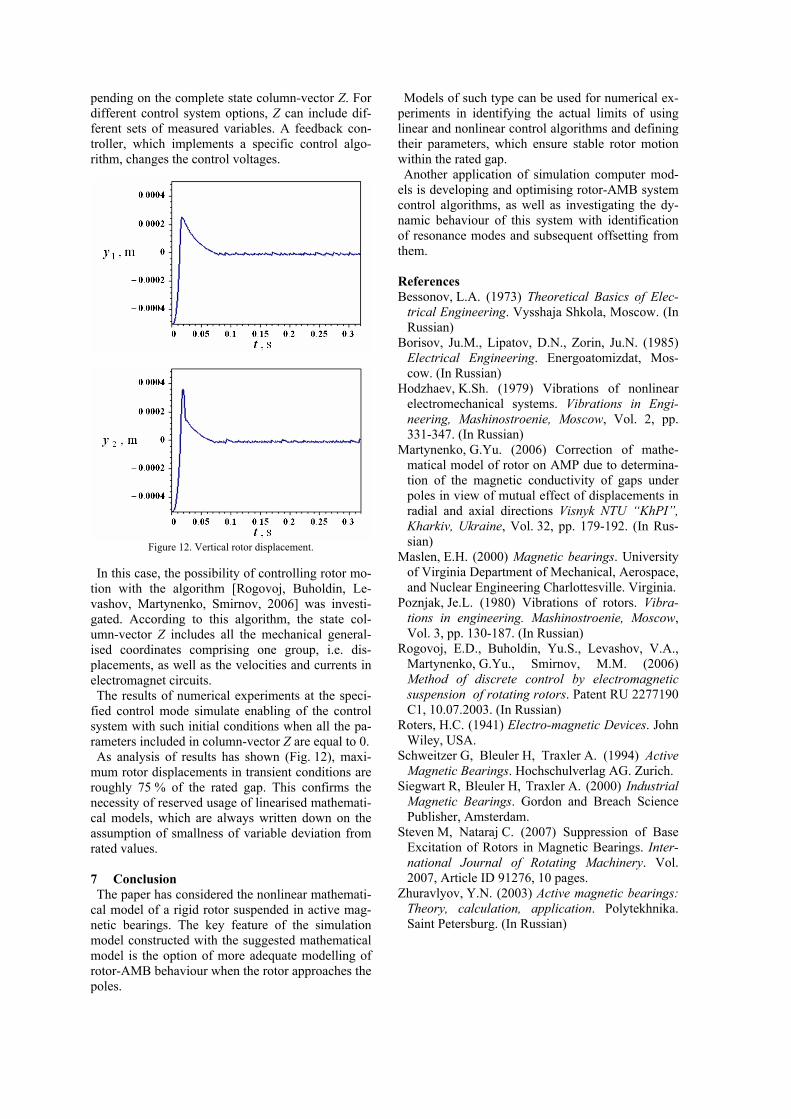
6 Numerical experiments The considered nonlinear mathematical model of a

suspension can serve as a basis of a simulation computer model (SCM) of a suspension for practical application in design research. Fig. 12 shows an example of calculating the dy-

namic behaviour of the rotor with the help of such an SCM. To obtain stable rotor motion in AMB, control

voltages uck should vary definitely with time de-

pending on the complete state column-vector Z. For different control system options, Z can include dif-ferent sets of measured variables. A feedback con-troller, which implements a specific control algo-rithm, changes the control voltages.

Figure 12. Vertical rotor displacement.

In this case, the possibility of controlling rotor mo-

tion with the algorithm [Rogovoj, Buholdin, Le-vashov, Martynenko, Smirnov, 2006] was investi-gated. According to this algorithm, the state col-umn-vector Z includes all the mechanical general-ised coordinates comprising one group, i.e. dis-placements, as well as the velocities and currents in electromagnet circuits. The results of numerical experiments at the speci-

fied control mode simulate enabling of the control system with such initial conditions when all the pa-rameters included in column-vector Z are equal to 0. As analysis of results has shown (Fig. 12), maxi-

mum rotor displacements in transient conditions are roughly 75 % of the rated gap. This confirms the necessity of reserved usage of linearised mathemati-cal models, which are always written down on the assumption of smallness of variable deviation from rated values.

7 Conclusion The paper has considered the nonlinear mathemati-

cal model of a rigid rotor suspended in active mag-netic bearings. The key feature of the simulation model constructed with the suggested mathematical model is the option of more adequate modelling of rotor-AMB behaviour when the rotor approaches the poles.

Models of such type can be used for numerical ex-periments in identifying the actual limits of using linear and nonlinear control algorithms and defining their parameters, which ensure stable rotor motion within the rated gap. Another application of simulation computer mod-

els is developing and optimising rotor-AMB system control algorithms, as well as investigating the dy-namic behaviour of this system with identification of resonance modes and subsequent offsetting from them.

References Bessonov, L.A. (1973) Theoretical Basics of Elec-

trical Engineering. Vysshaja Shkola, Moscow. (In Russian)

Borisov, Ju.M., Lipatov, D.N., Zorin, Ju.N. (1985) Electrical Engineering. Energoatomizdat, Mos-cow. (In Russian)

Hodzhaev, K.Sh. (1979) Vibrations of nonlinear electromechanical systems. Vibrations in Engi-neering, Mashinostroenie, Moscow, Vol. 2, pp. 331-347. (In Russian)

Martynenko, G.Yu. (2006) Correction of mathe-matical model of rotor on AMP due to determina-tion of the magnetic conductivity of gaps under poles in view of mutual effect of displacements in radial and axial directions Vіsnyk NTU “KhPI”, Kharkіv, Ukraine, Vol. 32, pp. 179-192. (In Rus-sian)

Maslen, E.H. (2000) Magnetic bearings. University of Virginia Department of Mechanical, Aerospace, and Nuclear Engineering Charlottesville. Virginia.

Poznjak, Je.L. (1980) Vibrations of rotors. Vibra-tions in engineering. Mashinostroenie, Moscow, Vol. 3, pp. 130-187. (In Russian)

Rogovoj, E.D., Buholdin, Yu.S., Levashov, V.A., Martynenko, G.Yu., Smirnov, M.M. (2006) Method of discrete control by electromagnetic suspension of rotating rotors. Patent RU 2277190 C1, 10.07.2003. (In Russian)

Roters, H.C. (1941) Electro-magnetic Devices. John Wiley, USA.

Schweitzer G, Bleuler H, Traxler A. (1994) Active Magnetic Bearings. Hochschulverlag AG. Zurich.

Siegwart R, Bleuler H, Traxler A. (2000) Industrial Magnetic Bearings. Gordon and Breach Science Publisher, Amsterdam.

Steven M, Nataraj C. (2007) Suppression of Base Excitation of Rotors in Magnetic Bearings. Inter-national Journal of Rotating Machinery. Vol. 2007, Article ID 91276, 10 pages.

Zhuravlyov, Y.N. (2003) Active magnetic bearings: Theory, calculation, application. Polytekhnika. Saint Petersburg. (In Russian)