Modelling the effects of air pollution on health using Bayesian dynamic generalised linear models

ENVIRONMETRICSEnvironmetrics 2008; 19: 785–804Published online 8 January 2008 in Wiley InterScience(www.interscience.wiley.com) DOI: 10.1002/env.894

Modelling the effects of air pollution on health using Bayesiandynamic generalised linear models

Duncan Lee1∗,† and Gavin Shaddick2

1University of Glasgow, Scotland, U.K.2University of Bath, Bath, U.K.

SUMMARY

The relationship between short-term exposure to air pollution and mortality or morbidity has been the subject ofmuch recent research, in which the standard method of analysis uses Poisson linear or additive models. In thispaper, we use a Bayesian dynamic generalised linear model (DGLM) to estimate this relationship, which allows thestandard linear or additive model to be extended in two ways: (i) the long-term trend and temporal correlation presentin the health data can be modelled by an autoregressive process rather than a smooth function of calendar time; (ii)the effects of air pollution are allowed to evolve over time. The efficacy of these two extensions are investigated byapplying a series of dynamic and non-dynamic models to air pollution and mortality data from Greater London.A Bayesian approach is taken throughout, and a Markov chain monte carlo simulation algorithm is presented forinference. An alternative likelihood based analysis is also presented, in order to allow a direct comparison with theonly previous analysis of air pollution and health data using a DGLM. Copyright © 2008 John Wiley & Sons, Ltd.

key words: dynamic generalised linear model; Bayesian analysis; Markov chain monte carlo simulation; airpollution

1. INTRODUCTION

The detrimental health effects associated with short-term exposure to air pollution is a major issue inpublic health, and the subject has received a great deal of attention in recent years. A number of epi-demiological studies have found positive associations between common pollutants, such as particulatematter (measured as PM10), ozone or carbon monoxide and mortality or morbidity, with many of theseassociations relating to pollution levels below existing guidelines and standards (see, e.g., Dominici etal., 2002; Vedal et al., 2003; Roberts, 2004). These associations have been estimated from single-site andmulti-city studies, the latter of which include ‘air pollution and health: a European approach’ (APHEA)(Zmirou et al., 1998) and ‘the national morbidity, mortality, and air pollution study’ (NMMAPS) (Sametet al., 2000). Although these studies have been conducted throughout the world in a variety of climates,positive associations have been consistently observed. The majority of these associations have beenestimated using time series regression methods, and as the health data are only available as daily counts,

∗Correspondence to: D. Lee, Department of Statistics, 15 University Gardens, University of Glasgow, G12 8QQ, U.K.†E-mail: [email protected]

Received 23 September 2006Copyright © 2008 John Wiley & Sons, Ltd. Accepted 2 October 2007

786 D. LEE AND G. SHADDICK

Poisson generalised linear and additive models are the standard method of analysis. These data relate tothe number of mortality or morbidity events that arise from the population living within a fixed region,for example a city, and are collected at daily intervals. Denoting the number of health events on day t

by yt , the standard log-linear model is given by:

yt ∼ Poisson(µt) for t = 1, . . . , n

ln(µt) = wtγ + zTt α (1)

in which the natural log of the expected health counts is linearly related to air pollution levels wt anda vector of r covariates, zT

t = (zt1, . . . , ztr). The covariates model any seasonal variation, long-termtrends and temporal correlation present in the health data, and typically include smooth functions ofcalendar time and meteorological variables, such as temperature. If the smooth functions are estimatedparametrically using regression splines, the model is linear, where as non-parametric estimation usingsmoothing splines, leads to an additive model.

In this paper we investigate the efficacy of using Bayesian dynamic generalised linear models(DGLMs, West et al., 1985; Fahrmeir and Tutz, 2001) to analyse air pollution and health data. DGLMsextend generalised linear models by allowing the regression parameters to evolve over time via anautoregressive process of order p, denoted AR(p). The autoregressive nature of such models suggeststwo changes from the standard model (1) described above. Firstly, long-term trends and temporal cor-relation, present in the health data, can be modelled with an autoregressive process, which is in contrastto the standard approach of using a smooth function of calendar time. Secondly, the effects of airpollution can be modelled with an autoregressive process, which allows these effects to evolve overtime. This evolution may be due to a change in the composition of individual pollutants, or becauseof a seasonal interaction with temperature. This is a comparatively new area of research, for whichPeng et al. (2005) and Chiogna and Gaetan (2002) are the only known studies in this setting. Thefirst of these forces the effects to follow a fixed seasonal pattern, which does not allow any othertemporal variation, such as a long-term trend. In contrast, Chiogna and Gaetan (2002) model this evo-lution as a first order random walk, which does not fix the temporal shape a-priori, allowing it tobe estimated from the data. Their work is the only known analysis of air pollution and health datausing DGLMs, and they implement their model in a likelihood framework using the Kalman filter.In this paper, we present a Bayesian analysis based on Markov chain monte carlo (MCMC) simula-tion, which we believe is a more natural framework in which to analyse hierarchical models of thistype.

The remainder of this paper is organised as follows. Section 2 introduces the Bayesian DGLMproposed here, and compares it to the likelihood based approach used by Chiogna and Gaetan (2002).Section 3 describes a Markov chain monte carlo estimation algorithm for the proposed model, whileSection 4 discusses the advantages of dynamic models for these data in more detail. Section 5 presentsa case study, which investigates the utility of dynamic models in this context by analysing data fromGreater London. Finally, Section 6 gives a concluding discussion and suggests areas for future work.

2. BAYESIAN DYNAMIC GENERALISED LINEAR MODELS

A Bayesian dynamic generalised linear model extends a generalised linear model by allowing a subset ofthe regression parameters to evolve over time as an autoregressive process. The general model proposed

Copyright © 2008 John Wiley & Sons, Ltd. Environmetrics 2008; 19: 785–804DOI: 10.1002/env

DYNAMIC MODELS FOR AIR POLLUTION AND HEALTH DATA 787

here begins with a Poisson assumption for the health data and is given by:


ln(µt) = xTt βt + zT

t α

βt = F1βt−1 + · · · + Fpβt−p + νt ; νt ∼ N(0, �β)

β0, . . . ,β−p+1 ∼ N(µ0, �0) (2)

α ∼ N(µα�α)

�β ∼ Inverse-Wishart(n�, S−1� )

The vector of health counts are denoted by y = (y1, . . . , yn)Tn×1, and the covariates include an r × 1

vector zt , with fixed parameters α = (α1, . . . , αr)Tr×1, and a q × 1 vector xt , with dynamic parameters

βt = (βt1, . . . , βtq)Tq×1. The dynamic parameters are assigned an autoregressive prior of order p, which isinitialised by starting parameters (β−p+1, . . . ,β0) at times (−p + 1, . . . , 0). Each initialising parameterhas a Gaussian prior with mean µ0q×1 and variance �0q×q , and are included to allow β1 to follow anautoregressive process. The autoregressive parameters can be stacked into a single vector denoted byβ = (β−p+1, . . . ,β0, β1, . . . , βn)T(n+p)q×1, and the variability in the process is controlled by a q × q

variance matrix �β, which is assigned a conjugate inverse-Wishart prior. For univariate processes �β isscalar, and the conjugate prior simplifies to an inverse-gamma distribution. The evolution and stationarityof this process are determined by �β and the q × q autoregressive matrices F = {F1, . . . , Fp}, the latterof which may contain unknown parameters or known constants, and the prior specification depends onits form. For example, a univariate first order autoregressive process is stationary if |F1| < 1, and a priorspecification is discussed in Section 3.1.4. A Gaussian prior is assigned to α because prior information issimple to specify in this form. The unknown parameters are (β, α, �β) and components of, F , whereasthe hyperparameters (µα, �α, n�, S�, µ0, �0) are known.

2.1. Estimation for a DGLM

We propose a Bayesian implementation of Equation (2) using MCMC simulation, because it providesa natural framework for inference in hierarchical models. However, numerous alternative approacheshave also been suggested, and a brief review is given here. West et al. (1985) proposed an approximateBayesian analysis based on relaxing the normality of the AR(1) process, and assuming conjugacybetween the data model and the AR(1) parameter model. They use Linear Bayes methods to estimatethe conditional moments of βt , while estimation of �β is circumvented using the discount method(Ameen and Harrison, 1985). Fahrmeir and co-workers (see Fahrmeir and Kaufmann, 1991; Fahrmeir,1992; Fahrmeir and Wagenpfeil, 1997) propose a likelihood based approach, which maximises the jointlikelihood f (β|y). They use an iterative algorithm that simultaneously updates β and �β, using theiteratively re-weighted Kalman filter and smoother, and expectation-maximisation (EM) algorithm (orgeneralised cross validation). This is the estimation approach taken by Chiogna and Gaetan (2002), anda comparison with our Bayesian implementation is given below. Other approaches to estimation includeapproximating the posterior density by piecewise linear functions (Kitagawa, 1987), using numericalintegration methods (Fruhwirth-Schnatter, 1994), and particle filters Kitagawa (1996).



2.2. Comparison with the likelihood based approach

The main difference between this work and that of Chiogna and Gaetan (2002), who also used a DGLMin this setting, is the approach taken to estimation and inference. We propose a Bayesian approach withanalysis based on MCMC simulation, which we believe has a number of advantages over the likelihoodbased analysis used by Chiogna and Gaetan. In a Bayesian approach the posterior distribution of β

correctly allows for the variability in the hyperparameters, while confidence intervals calculated in alikelihood analysis do not. In a likelihood analysis (�β, F ) are estimated by data driven criteria, such asgeneralised cross validation, and estimates and standard errors of β are calculated assuming (�β, F ) arefixed at their estimated values. As a result, confidence intervals for β are likely to be too narrow, whichmay lead to a statistically insignificant effect of air pollution appearing to be significant. In contrast,the Bayesian credible intervals are the correct width, because (β, �β, F ) are simultaneously estimatedwithin the MCMC algorithm.

The Bayesian approach allows the investigator to incorporate prior knowledge of the parameters intothe model, whilst results similar to a likelihood analysis can be obtained by specifying prior ignorance.This is particularly important in dynamic models because the regression parameters are likely to evolvesmoothly over time, and a non-informative prior for �β may result in the estimated parameter processbeing contaminated with unwanted noise. Such noise may hide a trend in the parameter process, and canbe removed by specifying an informative prior for �β. The Bayesian approach is the natural frameworkin which to view hierarchical models of this type, because it can incorporate variation at multiple levelsin a straightforward manner, whilst making use of standard estimation techniques. In addition, the fullposterior distribution can be calculated, whereas in a likelihood analysis only the mode and varianceare estimated. However, as with any Bayesian analysis computation of the posterior distribution is timeconsuming, and likelihood based estimation is quicker to implement. To assess the relative performanceof the two approaches, we apply all models in Section 5 using the Bayesian algorithm described inSection 3 and the likelihood based alternative used by Chiogna and Gaetan (2002).

The model proposed above is a re-formulation of that used by Chiogna and Gaetan (shown inEquation (3) below), which fits naturally within the Bayesian framework adopted here. Apart from theinclusion of prior distributions in the Bayesian approach, there are two major differences between thetwo models, the first of which is operational and the second is notational. Firstly, a vector of covariateswith fixed parameters (α) is explicitly included in the linear predictor, which allows the fixed anddynamic parameters to be updated separately in the MCMC simulation algorithm. This enables theautoregressive characteristics of β to be incorporated into its Metropolis-Hastings step, without forcingthe same autoregressive property onto the simulation of the fixed parameters. This would not be possiblein Equation (3) as covariates with fixed parameters are included in the AR(1) process by a particularspecification of �β and F (diagonal elements of �β are zero and F are one). This specification is alsoinefficient because n copies of each fixed parameter are estimated. Secondly, at first sight Equation(3) appears to be an AR(1) process which compares with our more general AR(p) process. In fact anAR(p) process can be written in the form of Equation (3) by a particular specification of (β, �β, F ),but we believe the approach given here is notationally clearer. In the next section we present an MCMCsimulation algorithm for carrying out inference within this Bayesian dynamic generalised linear model.


ln(µt) = xTt βt

βt = Fβt−1 + νt νt ∼ N(0, �β) (3)

β0 ∼ N(µ0, �0)



3. MCMC ESTIMATION ALGORITHM

The joint posterior distribution of (β, α, �β, F ) in Equation (2) is given by

f (β, α, �β, F |y) ∝ f (y|β, α, �β, F )f (α)f (β|�β, F )f (�β)f (F )

=n∏

t=1

Poisson(yt|βt , α)N(α|µα, �α)n∏

t=1

N(βt|F1βt−1 + · · · + Fpβt−p, �β)

× N(β−p+1|µ0, �0) . . . N(β0|µ0, �0)Inverse-Wishart(�β|nQ, S−1Q )f (F )

where f (F ) depends on the form of the AR(p) process. The next section describes the overall simulationalgorithm, with specific details given in Sections 3.1.1–3.1.4.

3.1. Overall simulation algorithm

The parameters are updated using a block Metropolis–Hastings algorithm, in which starting val-ues (β(0), α(0), �

(0)β , F (0)) are generated from overdispersed versions of the priors (for example t-

distributions replacing Gaussian distributions). The parameters are alternately sampled from their fullconditional distributions in the following blocks.

(a) Dynamic parameters β = (β−p+1, . . . ,βn).Further details are given in Section 3.1.1.

(b) Fixed parameters α = (α1, . . . , αr).Further details are given in Section 3.1.2.

(c) Variance matrix �β.Further details are given in Section 3.1.3.

(d) AR(p) matrices, F = (F1, . . . , Fp) (or components of).Further details are given in Section 3.1.4.

3.1.1. Sampling from f (β | y, α, Σβ, F ). The full conditional of β is the product of n Poisson observa-tions and a Gaussian AR(p) prior given by

f (β|y, α, �β, F ) ∝n∏

t=1

Poisson(yt|βt , α)n∏

t=1

N(βt|F1βt−1 + · · · + Fpβt−p, �β)

× N(β−p+1|µ0, �0) · · · N(β0|µ0, �0)

The full conditional is non-standard, and a number of simulation algorithms have been proposed, whichtake into account the autoregressive nature of β. Fahrmeir et al. (1992) combine a rejection sam-pling algorithm with a Gibbs step, but report acceptance rates that are very low making the algorithmprohibitively slow. In contrast, Shephard and Pitt (1997) and Gamerman (1998) suggest Metropolis–Hastings algorithms, in which the proposal distributions are based on Fisher scoring steps and Taylor



expansions, respectively. However, such proposal distributions are computationally expensive to calcu-late, and the conditional prior proposal algorithm of Knorr-Held (1999) is used instead. His proposaldistribution is computationally cheap to calculate, compared with those of Shephard and Pitt (1997)and Gamerman (1998), while the Metropolis–Hastings acceptance rate has a simple form and is easyto calculate. Further details are given in Appendix A.

3.1.2. Sampling from f (α|y, β, Σβ, F ). The full conditional of α is non-standard because it is theproduct of a Gaussian prior and n Poisson observations. As a result, simulation is carried out using aMetropolis–Hastings step, and two common choices are random walk and Fisher scoring proposals (fordetails see Fahrmeir and Tutz, 2001). A random walk proposal is used here because of its computationalcheapness compared with the Fisher scoring alternative, and the availability of a tuning parameter. Theparameters are updated in blocks, which is a compromise between the high acceptance rates obtainedby univariate sampling and the improved mixing that arises when large sets of parameters are sampledsimultaneously. Proposals are drawn from a Gaussian distribution with mean equal to the current valueof the block and a diagonal variance matrix. The diagonal variances are typically identical and can betuned to give good acceptance rates.

3.1.3. Sampling from f (Σβ|y, β, α, F ). The full conditional of �β comprises n AR(p) Gaussian dis-tributions for βt and a conjugate inverse-Wishart(n�, S−1

� ) prior, which results in an inverse-Wishart(a,b) posterior distribution with

a = n� + n

b =(

S� +n∑

t=1

(βt − F1βt−1 − · · · − Fpβt−p)(βt − F1βt−1 − · · · − Fpβt−p)T)−1

However, the models applied in Section 5 are based on univariate autoregressive processes, for whichthe conjugate prior simplifies to an inverse-gamma distribution. If a non-informative prior is required,an inverse-gamma(ε, ε) prior with small ε is typically used. However as discussed in Section 2.2, aninformative prior may be required for �β, and representing informative prior beliefs using a memberof the inverse-gamma family is not straightforward. The variance parameters of the autoregressiveprocesses are likely to be close to zero (to ensure the evolution is smooth), so we represent our priorbeliefs as a Gaussian distribution with zero mean, which is truncated to be positive. The informativenessof this prior is controlled by its variance, with smaller values resulting in a more informative distribution.If this prior is used, the full conditional can be sampled from using a Metropolis–Hastings step with arandom walk proposal.

3.1.4. Sampling from f (F | y, β, α, Σβ). The full conditional of F depends on the form and dimensionof the AR(p) process, and the most common types are univariate AR(1) (βt ∼ N(F1βt−1, �β)) andAR(2) (βt ∼ N(F1βt−1 + F2βt−2, �β)) processes. In either case, assigning (F1) or (F1, F2) flat priorsresults in a Gaussian full conditional distribution. For example in a univariate AR(1) process, the full

conditional for F1 is Gaussian with mean∑n

t=1βtβt−1∑n

t=1β2

t−1, and variance �β∑n

t=1β2

t−1. Similar results can be

found for an AR(2) process.



4. MODELLING AIR POLLUTION AND HEALTH DATA

As described in the introduction, air pollution and health data are typically modelled by Poisson linearor additive models, which are similar to Equation (1). The daily health counts are regressed against airpollution levels and a vector of covariates, the latter of which model long-term trends, seasonal variationand temporal correlation commonly present in the daily mortality series. The covariates typically includean intercept term, indicator variables for day of the week, and smooth functions of calendar time andmeteorological covariates, such as temperature. A large part of the seasonal variation is modelled by thesmooth function of temperature, while the long-term trends and temporal correlation are removed bythe smooth function of calendar time. The air pollution component typically has the form wtγ , whichforces its effect on health to be constant. Analysing these data with dynamic models allows this standardapproach to be extended in two ways, both of which are described below.

4.1. Modelling long-term trends and temporal correlation

The autoregressive nature of a dynamic generalised linear model, enables long-term trends and temporalcorrelation to be modelled by an autoregressive process, rather than a smooth function of calendar time.This is desirable because such a process sits in discrete time and estimates the underlying trend inthe data {t, yt}nt=1, while its smoothness is controlled by a single parameter (the evolution variance).In these respects an autoregressive process is a natural choice to model the influence of confoundingfactors because it can be seen as the discrete time analogue of a smooth function of calendar time. Inthe dynamic modelling literature (see e.g. Chatfield, 1996; Fahrmeir and Tutz, 2001), long-term trendsare commonly modelled by:

First order random walk βt ∼ N(βt−1, τ2)

Second order random walk βt ∼ N(2βt−1 − βt−2, τ2) (4)

Local linear trend model βt ∼ N(βt−1 + δt−1, τ2)

δt ∼ N(δt−1, ψ2).

All three processes are non-stationary which allows the underlying mean level to change over time, adesirable characteristic when modelling long-term trends. A second order random walk is the naturalchoice from the three alternatives, because it is the discrete time analogue of a natural cubic splineof calendar time (Fahrmeir and Tutz, 2001), one of the standard methods for estimating the smoothfunctions. Chiogna and Gaetan (2002) also use a second order random walk for this reason, but inSection 5 we extend their work by comparing the relative performance of smooth functions and each ofthe three processes listed above. We estimate the smooth function with a natural cubic spline, becauseit is parametric, making estimation within a Bayesian setting straightforward.

4.2. Modelling the effects of air pollution

The effects of air pollution are typically assumed to be constant (represented by γ), or depend on thelevel of air pollution, the latter of which replaces wtγ in Equation (1) with a smooth function f (wt|λ).This is called a dose–response relationship, and higher pollution levels typically result in larger adverseeffects. Comparatively little research has allowed these effects to evolve over time, and any temporalvariation is likely to be seasonal or exhibit a long-term trend. Seasonal effects may be caused byan interaction with temperature, or with another pollutant exhibiting a seasonal pattern. In contrast,



long-term trends may result from a slow change in the composition of harmful pollutants, or from achange in the size and structure of the population at risk over a number of years. The only previous studieswhich investigate the time-varying effects of air pollution are those of Peng et al. (2005) and Chiogna andGaetan (2002), who model the temporal evolution as γt = θ0 + θ1 sin(2πt/365) + θ2 cos(2πt/365) andγt ∼ N(γt−1, σ

2), respectively. The seasonal form is restrictive because it does not allow the temporalvariation to exhibit shapes which are not seasonal. In contrast, the first order random walk used byChiogna and Gaetan (2002) does not fix the form of the time-varying effects a-priori, allowing theirshape to be estimated from the data, which results in a more realistic model. In Section 5, we also modelthis temporal variation with a first order random walk, because of its flexibility and because it allows acomparison with the work of Chiogna and Gaetan (2002).

5. CASE STUDY ANALYSING DATA FROM GREATER LONDON

The extensions to the standard model described in Section 4 are investigated by analysing data fromGreater London. The first subsection describes the data that are used in this case study, the seconddiscusses the choice of statistical models, while the third presents the results.

5.1. Description of the data

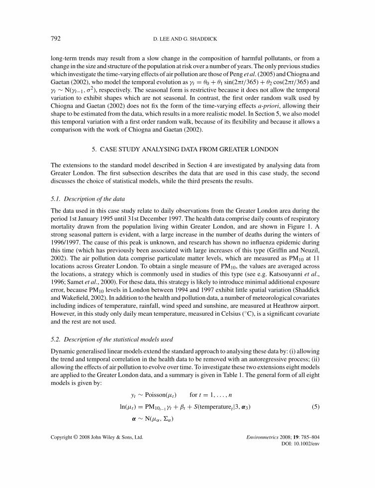
The data used in this case study relate to daily observations from the Greater London area during theperiod 1st January 1995 until 31st December 1997. The health data comprise daily counts of respiratorymortality drawn from the population living within Greater London, and are shown in Figure 1. Astrong seasonal pattern is evident, with a large increase in the number of deaths during the winters of1996/1997. The cause of this peak is unknown, and research has shown no influenza epidemic duringthis time (which has previously been associated with large increases of this type (Griffin and Neuzil,2002). The air pollution data comprise particulate matter levels, which are measured as PM10 at 11locations across Greater London. To obtain a single measure of PM10, the values are averaged acrossthe locations, a strategy which is commonly used in studies of this type (see e.g. Katsouyanni et al.,1996; Samet et al., 2000). For these data, this strategy is likely to introduce minimal additional exposureerror, because PM10 levels in London between 1994 and 1997 exhibit little spatial variation (Shaddickand Wakefield, 2002). In addition to the health and pollution data, a number of meteorological covariatesincluding indices of temperature, rainfall, wind speed and sunshine, are measured at Heathrow airport.However, in this study only daily mean temperature, measured in Celsius (◦C), is a significant covariateand the rest are not used.

5.2. Description of the statistical models used

Dynamic generalised linear models extend the standard approach to analysing these data by: (i) allowingthe trend and temporal correlation in the health data to be removed with an autoregressive process; (ii)allowing the effects of air pollution to evolve over time. To investigate these two extensions eight modelsare applied to the Greater London data, and a summary is given in Table 1. The general form of all eightmodels is given by:


ln(µt) = PM10t−1γt + βt + S(temperaturet|3, α3) (5)

α ∼ N(µα, �α)



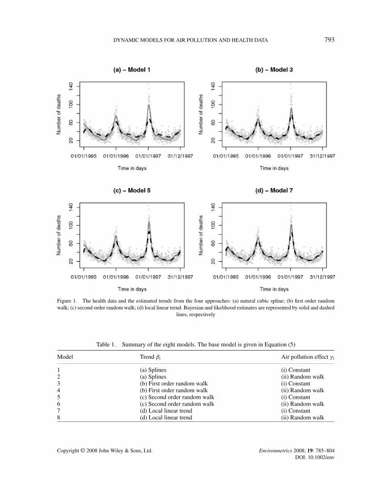
Figure 1. The health data and the estimated trends from the four approaches: (a) natural cubic spline; (b) first order randomwalk; (c) second order random walk; (d) local linear trend. Bayesian and likelihood estimates are represented by solid and dashed

lines, respectively

Table 1. Summary of the eight models. The base model is given in Equation (5)

Model Trend βt Air pollution effect γt

1 (a) Splines (i) Constant2 (a) Splines (ii) Random walk3 (b) First order random walk (i) Constant4 (b) First order random walk (ii) Random walk5 (c) Second order random walk (i) Constant6 (c) Second order random walk (ii) Random walk7 (d) Local linear trend (i) Constant8 (d) Local linear trend (ii) Random walk



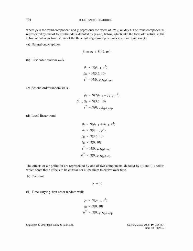
where βt is the trend component, and γt represents the effect of PM10 on day t. The trend component isrepresented by one of four submodels, denoted by (a)–(d) below, which take the form of a natural cubicspline of calendar time or one of the three autoregressive processes given in Equation (4).

(a) Natural cubic splines

βt = α1 + S(t|k, α2);

(b) First order random walk

βt ∼ N(βt−1, τ2)

β0 ∼ N(3.5, 10)

τ2 ∼ N(0, g2)I[τ2>0];

(c) Second order random walk

βt ∼ N(2βt−1 − βt−2, τ2)

β−1, β0 ∼ N(3.5, 10)

τ2 ∼ N(0, g3)I[τ2>0];

(d) Local linear trend

βt ∼ N(βt−1 + δt−1, τ2)

δt ∼ N(δt−1, ψ2)

β0 ∼ N(3.5, 10)

δ0 ∼ N(0, 10)

τ2 ∼ N(0, g4)I[τ2>0]

ψ2 ∼ N(0, g5)I[ψ2>0].

The effects of air pollution are represented by one of two components, denoted by (i) and (ii) below,which force these effects to be constant or allow them to evolve over time.

(i) Constant

γt = γ;

(ii) Time-varying–first order random walk

γt ∼ N(γt−1, σ2)

γ0 ∼ N(0, 10)

σ2 ∼ N(0, g1)I[σ2>0].



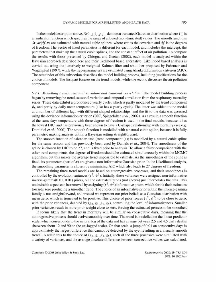
In the model description above, N(0, g1)I[σ2>0] denotes a truncated Gaussian distribution where I[ ] isan indicator function which specifies the range of allowed (non-truncated) values. The smooth functionsS(var|df, α) are estimated with natural cubic splines, where var is the covariate and df is the degreesof freedom. The vector of fixed parameters is different for each model, and includes the intercept, theparameters that make up the natural cubic splines, and the constant effect of air pollution. To comparethe results with those presented by Chiogna and Gaetan (2002), each model is analysed within theBayesian approach described here and their likelihood based alternative. Likelihood based analysis iscarried out using the iteratively re-weighted Kalman filter and smoother proposed by Fahrmeir andWagenpfeil (1997), while the hyperparameters are estimated using Akaike information criterion (AIC).The remainder of this subsection describes the model building process, including justifications for thechoice of models. The first part focuses on the trend models, while the second discusses the air pollutioncomponent.

5.2.1. Modelling trends, seasonal variation and temporal correlation. The model building processbegan by removing the trend, seasonal variation and temporal correlation from the respiratory mortalityseries. These data exhibit a pronounced yearly cycle, which is partly modelled by the trend componentβt , and partly by daily mean temperature (also has a yearly cycle). The latter was added to the modelat a number of different lags with different shaped relationships, and the fit to the data was assessedusing the deviance information criterion (DIC, Spiegelalter et al., 2002). As a result, a smooth functionof the same days temperature with three degrees of freedom is used in the final models, because it hasthe lowest DIC, and has previously been shown to have a U-shaped relationship with mortality (see e.g.Dominici et al., 2000). The smooth function is modelled with a natural cubic spline, because it is fullyparametric making analysis within a Bayesian setting straightforward.

The smooth function of calendar time (trend component (a)) is modelled by a natural cubic splinefor the same reason, and has previously been used by Daniels et al., 2004). The smoothness of thespline is chosen by DIC to be 27, and is fixed prior to analysis. To allow a fairer comparison with theother trend components, the degrees of freedom should be estimated simultaneously within the MCMCalgorithm, but this makes the average trend impossible to estimate. As the smoothness of the spline isfixed, its parameters (part of α) are given a non-informative Gaussian prior. In the Likelihood analysis,the smoothing parameter is chosen by minimising AIC which also leads to 27 degrees of freedom.

The remaining three trend models are based on autoregressive processes, and their smoothness iscontrolled by the evolution variances (τ2, ψ2). Initially, these variances were assigned non-informativeinverse-gamma(0.01, 0.01) priors, but the estimated trends (not shown) just interpolates the data. Thisundesirable aspect can be removed by assigning (τ2, ψ2) informative priors, which shrink their estimatestowards zero producing a smoother trend. The choice of an informative prior within the inverse-gammafamily is not straightforward, and instead we represent our prior beliefs as a Gaussian distribution withmean zero, which is truncated to be positive. This choice of prior forces (τ2, ψ2) to be close to zero,with the prior variances, denoted by (g2, g3, g4, g5), controlling the level of informativeness. Smallerprior variances result in more prior weight close to zero, forcing the estimated process to be smoother.

It seems likely that the trend in mortality will be similar on consecutive days, meaning that theautoregressive process should evolve smoothly over time. The trend is modelled on the linear predictorscale, which corresponds to the natural log of the data and has a range between 2.5 and 4.5 daily deaths(between about 12 and 90 on the un-logged scale). On that scale, a jump of 0.01 on consecutive days isapproximately the largest difference that cannot be detected by the eye, resulting in a visually smoothtrend. To relate this to the choice of (g2, g3, g4, g5), each of the three processes were simulated witha variety of variances, and the average absolute difference between consecutive values was calculated.



The variances were chosen so that 50% of the prior mass was below the threshold value that gaveaverage differences of 0.01, resulting in g2 = 10−7, g3 = 10−14. The local linear trend model has twovariance parameters, and it was found that both needed to be tightly controlled for the process to evolvesmoothly, resulting in g4 = g5 = 10−16. Sensitivity analyses were carried out for different values of(g2, g3, g4, g5), but it was found that larger values resulted in trends that were not visually smooth.In the likelihood analysis, the variance parameters are chosen by optimising AIC. The priors for theinitialising parameters (β−1, β0, δ0) are non-informative Gaussian distributions with mean equal to zerofor the rate δ0, and 3.5 for (β−1, β0), the average of mortality data from previous years on the loggedscale.

5.2.2. Modelling the effects of PM10. After modelling the influence of unmeasured risk factors, theeffects of PM10 at a number of different lags were investigated. A lag of one day is used in the finalmodels, because it has the minimum DIC and has been used in other recent studies (see e.g. Dominiciet al., 2000; Zhu et al., 2003). Constant and time-varying effects of PM10 are investigated in this casestudy, with the latter modelled by a first order random walk, which allows a comparison with the work ofChiogna and Gaetan (2002). Initially, a non-informative inverse-gamma(0.01, 0.01) prior was specifiedfor the variance of the random walk (denoted by σ2), but the estimated time-varying effects (not shown)are contaminated by noise and an underlying trend cannot be seen. These effects are likely to evolvesmoothly over time, and to enforce this smoothness σ2 is assigned an informative zero mean Gaussianprior which is truncated to be positive. The informativeness is controlled by the variance g1, which ischosen using an identical approach to that described above. In this case the likely range of effects is−0.003 to 0.005, and the largest difference that is undetectable by the eye is around 0.00005, leadingto g1 = 10−16. To corroborate this choice a sensitivity analysis was carried out for different values ofg1, which showed the evolution was smooth for values as large as 10−10. As this is less informativethan 10−16, it is used in the final models. In the likelihood analysis, the variance parameter is chosenby optimising the AIC.

5.3. Results

The models contain a large number of parameters, so to aid convergence the covariates (PM10 and thebasis functions for the natural cubic splines of calendar time and temperature) are standardised to have amean of zero and a standard deviation of one before inclusion in the model (and are subsequently back-transformed when obtaining results from the posterior distribution). The Markov chains are burnt in for40 000 iterations, by which point convergence was assessed to have been reached using the methods ofGelman et al. (2003). At this point a further 100 000 iterations are simulated, which are thinned by 5 toreduce autocorrelation, resulting in 20 000 samples from the joint posterior distribution.

5.3.1. Results for the four trend models βt . Long-term trends, overdispersion and temporal correlationare removed from the health data with one of four trend models: a natural cubic spline of calendartime (models 1 and 2); a first order random walk (models 3 and 4); a second order random walk(models 5 and 6) and a local linear trend model (models 7 and 8). To aid clarity in the followingdiscussion, these approaches are compared and contrasted assuming a constant effect of air pollution(using the odd numbered models). Figure 1 shows the health data from Greater London, together withthe estimated trends from the Bayesian (solid lines) and likelihood (dotted lines) analyses. Panel (a)shows the estimated trend from a natural cubic spline of calendar time, panel (b) relates to the first orderrandom walk, panel (c) to the second order random walk, and panel (d) to the local linear trend model.



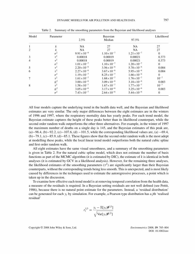
Table 2. Summary of the smoothing parameters from the Bayesian and likelihood analyses

Model Parameter Bayesian Likelihood2.5% Median 97.5%

1 k NA 27 NA 272 k NA 27 NA 27

σ2 9.91×10−8 1.10×10−7 1.21×10−7 03 τ2 0.00018 0.00019 0.00021 0.3734 τ2 0.00018 0.00019 0.00021 0.373

σ2 1.01×10−7 1.10×10−7 1.20×10−7 05 τ2 2.20×10−6 3.56×10−6 5.78×10−6 0.0046 τ2 2.27×10−6 3.67×10−6 5.95×10−6 0.004

σ2 1.19×10−7 8.25×10−7 1.66×10−6 07 τ2 1.61×10−7 1.68×10−7 1.76×10−7 10−7

ψ2 3.00×10−6 3.09×10−6 3.18×10−6 0.0038 τ2 1.58×10−7 1.67×10−7 1.77×10−7 10−7

ψ2 3.05×10−6 3.17×10−6 3.25×10−6 0.003σ2 7.43×10−7 2.64×10−6 5.44×10−6 0

All four models capture the underlying trend in the health data well, and the Bayesian and likelihoodestimates are very similar. The only major differences between the eight estimates are in the wintersof 1996 and 1997, where the respiratory mortality data has yearly peaks. For each trend model, theBayesian estimate captures the height of these peaks better than its likelihood counterpart, while thesecond order random walk outperforms the other three alternatives. For example, in the winter of 1997the maximum number of deaths on a single day is 145, and the Bayesian estimates of this peak are,(a)−98.4, (b)−92.2, (c)−107.6, (d) −101.5, while the corresponding likelihood values are, (a) −69.4,(b)−79.1, (c)−85.9, (d)−85.1. These figures show that the second order random walk is the most adeptat modelling these peaks, while the local linear trend model outperforms both the natural cubic splineand first order random walk.

All eight estimates have the same visual smoothness, and a summary of the smoothing parametersis given in Table 2. For the natural cubic spline model, which does not estimate the number of basisfunctions as part of the MCMC algorithm (it is estimated by DIC), the estimate of k is identical in bothanalyses (it is estimated by GCV in a likelihood analysis). However, for the remaining three analyses,the likelihood estimates of the smoothing parameters (τ2) are significantly larger than their Bayesiancounterparts, without the corresponding trends being less smooth. This is unexpected, and is most likelycaused by differences in the techniques used to estimate the autoregressive processes, a point which istaken up in the discussion.

To examine how effective each trend model is at removing temporal correlation from the health data,a measure of the residuals is required. In a Bayesian setting residuals are not well defined (see Pettit,1986), because there is no natural point estimate for the parameters. Instead, a ‘residual distribution’can be generated for each yt by simulation. For example, a Pearson type distribution has a jth ‘realisedresidual’

r(j)t = yt − E[yt|θ(j)]√

Var[yt|θ(j)]



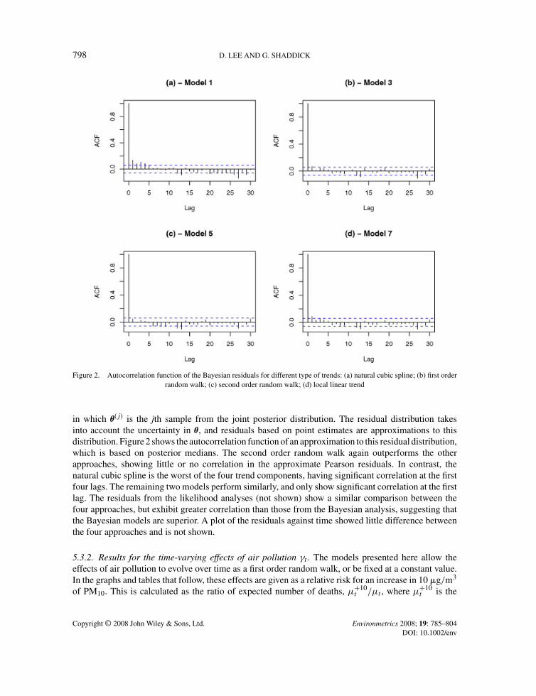
Figure 2. Autocorrelation function of the Bayesian residuals for different type of trends: (a) natural cubic spline; (b) first orderrandom walk; (c) second order random walk; (d) local linear trend

in which θ(j) is the jth sample from the joint posterior distribution. The residual distribution takesinto account the uncertainty in θ, and residuals based on point estimates are approximations to thisdistribution. Figure 2 shows the autocorrelation function of an approximation to this residual distribution,which is based on posterior medians. The second order random walk again outperforms the otherapproaches, showing little or no correlation in the approximate Pearson residuals. In contrast, thenatural cubic spline is the worst of the four trend components, having significant correlation at the firstfour lags. The remaining two models perform similarly, and only show significant correlation at the firstlag. The residuals from the likelihood analyses (not shown) show a similar comparison between thefour approaches, but exhibit greater correlation than those from the Bayesian analysis, suggesting thatthe Bayesian models are superior. A plot of the residuals against time showed little difference betweenthe four approaches and is not shown.

5.3.2. Results for the time-varying effects of air pollution γt . The models presented here allow theeffects of air pollution to evolve over time as a first order random walk, or be fixed at a constant value.In the graphs and tables that follow, these effects are given as a relative risk for an increase in 10 �g/m3

of PM10. This is calculated as the ratio of expected number of deaths, µ+10t /µt , where µ+10

t is the



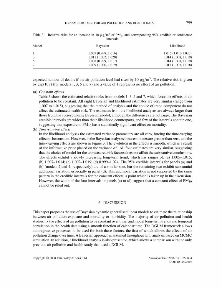
Table 3. Relative risks for an increase in 10 �g/m3 of PM10 and corresponding 95% credible or confidenceintervals

Model Bayesian Likelihood

1 1.007 (0.998, 1.016) 1.015 (1.010,1.020)3 1.011 (1.002, 1.020) 1.014 (1.008, 1.019)5 1.008 (0.999, 1.017) 1.014 (1.008, 1.019)7 1.009 (1.000, 1.019) 1.013 (1.007, 1.018)

expected number of deaths if the air pollution level had risen by 10 �g/m3. The relative risk is givenby exp(10γ) (for models 1, 3, 5 and 7) and a value of 1 represents no effect of air pollution.

(a) Constant effectsTable 3 shows the estimated relative risks from models 1, 3, 5 and 7, which force the effects of airpollution to be constant. All eight Bayesian and likelihood estimates are very similar (range from1.007 to 1.015), suggesting that the method of analysis and the choice of trend component do notaffect the estimated health risk. The estimates from the likelihood analyses are always larger thanthose from the corresponding Bayesian model, although the differences are not large. The Bayesiancredible intervals are wider than their likelihood counterparts, and few of the intervals contain one,suggesting that exposure to PM10 has a statistically significant effect on mortality.

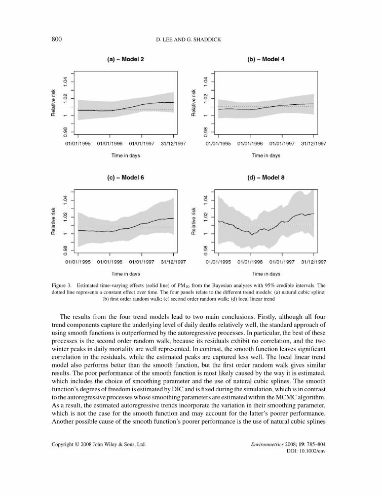
(b) Time-varying effectsIn the likelihood analyses the estimated variance parameters are all zero, forcing the time-varyingeffect to be constant. However, in the Bayesian analyses these estimates are greater than zero, and thetime-varying effects are shown in Figure 3. The evolution in the effects is smooth, which is a resultof the informative prior placed on the variance σ2. All four estimates are very similar, suggestingthat the choice of model for the unmeasured risk factors does not affect the substantive conclusions.The effects exhibit a slowly increasing long-term trend, which has ranges of: (a) 1.005–1.015;(b) 1.007–1.014; (c) 1.002–1.019; (d) 0.999–1.024. The 95% credible intervals for panels (a) and(b) (models 2 and 4, respectively) are of a similar size, but the remaining two exhibit substantialadditional variation, especially in panel (d). This additional variation is not supported by the samepattern in the credible intervals for the constant effects, a point which is taken up in the discussion.However, the width of the four intervals in panels (a) to (d) suggest that a constant effect of PM10cannot be ruled out.

6. DISCUSSION

This paper proposes the use of Bayesian dynamic generalised linear models to estimate the relationshipbetween air pollution exposure and mortality or morbidity. The majority of air pollution and healthstudies fix the effects of air pollution to be constant over time, and model long-term trends and temporalcorrelation in the health data using a smooth function of calendar time. The DGLM framework allowsautoregressive processes to be used for both these factors, the first of which allows the effects of airpollution change over time. A Bayesian approach is assumed throughout with analysis based on MCMCsimulation. In addition, a likelihood analysis is also presented, which allows a comparison with the onlyprevious air pollution and health study that used a DGLM.



Figure 3. Estimated time-varying effects (solid line) of PM10 from the Bayesian analyses with 95% credible intervals. Thedotted line represents a constant effect over time. The four panels relate to the different trend models: (a) natural cubic spline;

(b) first order random walk; (c) second order random walk; (d) local linear trend

The results from the four trend models lead to two main conclusions. Firstly, although all fourtrend components capture the underlying level of daily deaths relatively well, the standard approach ofusing smooth functions is outperformed by the autoregressive processes. In particular, the best of theseprocesses is the second order random walk, because its residuals exhibit no correlation, and the twowinter peaks in daily mortality are well represented. In contrast, the smooth function leaves significantcorrelation in the residuals, while the estimated peaks are captured less well. The local linear trendmodel also performs better than the smooth function, but the first order random walk gives similarresults. The poor performance of the smooth function is most likely caused by the way it is estimated,which includes the choice of smoothing parameter and the use of natural cubic splines. The smoothfunction’s degrees of freedom is estimated by DIC and is fixed during the simulation, which is in contrastto the autoregressive processes whose smoothing parameters are estimated within the MCMC algorithm.As a result, the estimated autoregressive trends incorporate the variation in their smoothing parameter,which is not the case for the smooth function and may account for the latter’s poorer performance.Another possible cause of the smooth function’s poorer performance is the use of natural cubic splines



to estimate it. Regression splines were used here because of their parametric make-up, but are knownto be less flexible than non-parametric alternatives. An interesting area of future research would be tocompare the performances of the trend models used here, against non-parametric smooth functions,such as smoothing splines or LOESS smoothers.

Secondly, the Bayesian approach gives results that are superior to the likelihood analysis, both interms of removing temporal correlation from the health data, and its ability to capture winter peaksin mortality. The estimated smoothing parameters for the Bayesian and likelihood implementations ofthe natural cubic splines are obtained by optimising data driven criteria (DIC and AIC), and it is notsurprising that both estimates are identical. However, for the autoregressive processes the Bayesianestimates are smaller than their likelihood counterparts, which is caused by the relative strengths ofthe truncated Gaussian prior and the penalty term in the AIC criteria. A sensitivity analysis shows thatsuch a strong prior is required, because using a non-informative prior for τ2 results in the estimatedtrend interpolating the data. An initial comparison of the estimated smoothing parameters (τ2) for theBayesian and likelihood analyses, shows that the latter were larger and therefore might be expected toproduce a trend exhibiting greater variability (and thus model the data at the peaks more accurately).However, the opposite was observed, and the larger estimates of τ2 in the likelihood analyses result intrends which are less variable. This apparent anomaly is most likely caused by differences in the methodsused to implement the autoregressive constraint for β. In the Bayesian analysis, this is implementedthrough the specification of an autoregressive prior f (β), whereas the likelihood approach enforcesthe autoregressive constraint using the Kalman filter. The filter uses a two stage process which firstlyestimates E[βt|y1, . . . , yt], for all t, and then smoothes the results by estimating E[βt|y1, . . . , yn].The final likelihood estimates are based on these smoothed values, and it is this additional smoothingimposed by the Kalman filter, that reduces the variability in the estimated trends, which over smoothesthe data in this case.

The Bayesian estimates of the pollution–mortality relationship exhibit a consistent long-term patternregardless of the choice of trend model, suggesting that this temporal variation should be investigatedfurther. However, no seasonal interaction is observed, meaning that the model of Peng et al. (2005) istoo restrictive for these data. The informative prior for σ2 forces these effects to evolve smoothly overtime, while a sensitivity analysis showed that using a non-informative prior leads to the estimate beingcontaminated with noise. This noise is caused by the excess number of parameters used to model thetime-varying effects, which makes these parameters non-identifiable. A non-informative prior for σ2

is too weak for these data, and the specification of an informative prior shrinks the evolution variancetowards zero, effectively reducing the number of parameters. The resulting temporal evolution is smooth,but this is achieved at the expense of a very informative prior.

The estimated time-varying effects are not altered by the choice of trend model, although the credibleintervals increase in width if a second order random walk or local linear trend are used. These two rep-resent the most flexible trend models, and their increased variation may cause slight non-identifiabilityor collinearity with the time-varying effects of PM10, reducing their precision. The estimated temporalvariation from the Bayesian models exhibit a similar shape to those reported by Chiogna and Gaetan(2002) in Birmingham Alabama, using a likelihood approach. However, this contrasts with our like-lihood based analyses which forced the effects to be constant and not exhibit any temporal variation.The difference in curvature between our Bayesian and likelihood analyses is again due to the way thesmoothing parameters are estimated. The likelihood approach calculates the likelihood for a range ofvalues of the smoothing parameter, and estimates σ2 by optimising a data driven criterion. In contrast,the Bayesian approach averages over the posterior for σ2, which incorporates the possibility of nosmoothing, thus leading to an estimate which exhibits greater curvature.



ACKNOWLEDGEMENTS

We would like to thank the Small Area Health Statistics Unit, which is funded by grants from the Department ofHealth, Department of the Environment, Food and Rural Affairs, Health and Safety Executive, Scottish Executive,National Assembly of Wales and Northern Ireland Assembly, who provided the mortality data from Greater London.

REFERENCES

Ameen J, Harrison P. 1985. Normal discount bayesian models. Bayesian Statistics 2 2: 271–198.Chatfield C. 1996. The Analysis of Time Series: An Introduction, 5th edn. Chapman and Hall: London.Chiogna M, Gaetan C. 2002. Dynamic generalized linear models with applications to environmental epidemiology. Applied

Statistics 51: 453–468.Daniels M, Dominici F, Zeger S, Samet J. 2004. The national morbidity, mortality, and air pollution study part III: concentration–

response curves and thresholds for the 20 largest US cities. HEI Project 96–97: 1–21.Dominici F, Daniels M, Zeger S, Samet J. 2002. Air pollution and mortality: estimating regional and national dose-response

relationships. Journal of the American Statistical Association 97: 100–111.Dominici F, Samet J, Zeger S. 2000. Combining evidence on air pollution and daily mortality from the 20 largest US cities: a

hierarchical modelling strategy. Journal of the Royal Statistical Society series A 163: 263–302.Fahrmeir L. 1992. Posterior mode estimation by extended Kalman filtering for multivariate dynamic generalized linear models.

Journal of the American Statistical Association 87: 501–509.Fahrmeir L, Hennevogl W, Klemme K. 1992. Smoothing in dynamic generalized linear models by Gibbs sampling. Advances in

GLIM and Statistical Modelling. Springer: Heidelberg.Fahrmeir L, Kaufmann H. 1991. On Kalman filtering, posterior mode estimation and fisher scoring in dynamic exponential family

regression. Metrika 38: 37–60.Fahrmeir L, Tutz G. 2001. Multivariate Statistical Modelling Based on Generalized Linear Models, 2nd edn. Springer: New York

and Berlin.Fahrmeir L, Wagenpfeil S. 1997. Penalized likelihood estimation and iterative Kalman smoothing for non-Gaussian dynamic

regression models. Computational Statistics and Data Analysis 24: 295–320.Fruhwirth-Schnatter S. 1994. Applied state space modelling of non-Gaussian time series using integration-based Kalman filtering.

Statistics and Computing 4: 259–269.Gamerman D. 1998. Markov chain Monte Carlo for dynamic generalized linear models. Biometrika 85: 215–227.Gelman A, Carlin J, Stern H, Rubin D. 2003. Bayesian Data Analysis, 2nd edn. Chapman and Hall: London.Griffin M, Neuzil K. 2002. The global implications of influenza in Hong Kong. The New England Journal Of Medicine 347:

2159–2162.Katsouyanni K, Schwartz J, Spix C, Touloumi G, Zmirou D, Zanobetti A, Wojtyniak B, Vonk J, Tobias A, Ponka A, Medina S,

Bacharove L, Anderson H. 1996. Short term effects of air pollution on health: a European approach using epidemiologic timeseries data: the APHEA protocol. Journal of Epidemiology and Community Health 50: S12–S18.

Kitagawa G. 1987. Non-Gaussian state-space modelling of nonstationary time series. Journal of the American Statistical Asso-ciation 82: 1032–1041.

Kitagawa G. 1996. Monte Carlo filter and smoother for non-Gaussian nonlinear state-space models. Journal of Computationaland Graphical Statistics 5: 1–25.

Knorr-Held L. 1999. Conditional prior proposals in dynamic models. Scandinavian Journal of Statistics 26: 129–144.Peng R, Dominici F, Pastor-Barriuso R, Zeger S, Samet J. 2005. Seasonal analyses of air pollution and mortality in 100 U.S.

cities. American Journal of Epidemiology 161: 585–594.Pettit L. 1986. Diagnostics in Bayesian model choice. The Statistician 35: 183–190.Roberts S. 2004. Biologically plausible particulate air pollution mortality concentration–response functions. Environmental Health

Perspectives 112: 309–313.Samet J, Zeger S, Dominici F, Curriero F, Coursac I, Dockery D, Schwartz J, Zanobetti A. 2000. The national morbidity, mortality,

and air pollution study part II: morbidity and mortality, from air pollution in the United States. HEI Project 96–97: 5–47.Shaddick G, Wakefield J. 2002. Modelling multiple pollutants and multiple sites. Applied Statistics 51: 351–372.Shephard N, Pitt M. 1997. Likelihood analysis of non-Gaussian measurement time series. Biometrika 84: 653–667.Spiegelalter D, Best N, Carlin B, Van der Linde A. 2002. Bayesian measures of model complexity and fit. Journal of the Royal

Statistical Society series B 64: 583–639.Vedal S, Brauer M, White R, Petkau J. 2003. Air pollution and daily mortality in a city with low levels of pollution. Environmental

Health Perpespectives 111: 45–51.West M, Harrison J, Migon H. 1985. Dynamic generalized linear models and bayesian forecasting. Journal of the American

Statistical Association 80: 73–83.



Zhu L, Carlin B, Gelfand A. 2003. Hierarchical regression with misaligned spatial data: relating ambient ozone and pediatricasthma ER visits in Atlanta. Environmetrics 14: 537–557.

Zmirou D, Schwartz J, Saez M, Zanobetti A, Wojtyniak B, Touloumi G, Spix C, Ponce de Leon A, Le Moullec Y, Bacharova L,Schouten J, Ponka A, Katsouyanni K. 1998. Time-series analysis of air pollution and cause specific mortality. Epidemiology9: 495–503.

APPENDIX A: SIMULATION OF β

The first p parameters are updated separately from β1, . . . ,βn, because their full conditional distributiondoes not depend on y and is a standard Gaussian distribution. In contrast, β1, . . . ,βn are sampled usinga block Metropolis–Hastings scheme, in which the proposal distribution is based on the autoregressiveprior. Ignoring β−p+1, . . . , β0 which have already been sampled, the autoregressive prior can be writtenas a singular multivariate Gaussian distribution

f (β|F, �β) =n∏

t=1

N(βt|F1βt−1 + · · · + Fpβt−p, �β)

∝ exp

(−1

2βT Kβ

)

with mean zero and singular precision matrix K. The precision matrix is given by

K =

K−p+1,−p+1 . . . K−p+1,n

......

Kn,−p+1 . . . Kn,n

(n+p)q×(n+p)q

where Kt,t is a q × q block relating to βt . The blocks depend on the order of the AR(p) process, andK has a bandwidth of p blocks (all blocks Kij , for which |i − j| > p are zero). For example, an AR(1)process leads to

Kt,t =

FT1 �−1

β F1 t = 0

FT1 �−1

β F1 + �−1β t = 1, . . . , n − 1

�−1β t = n

Kt,t+1 = −FT1 �−1

β ∀ t

Kt,t−1 = −�−1β F1 ∀ t

The parameters are updated in blocks of size g, which is used as a tuning parameter to achieve the desiredacceptance rates. The proposal distribution for a block βr,s = (βr, . . . ,βs)gq×1 in which s = r + g − 1is given by

f (βr,s|β−r,s, F, �β) ∼ N(µr,s, �r,s)



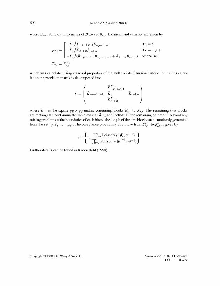
where β−r,s denotes all elements of β except βr,s. The mean and variance are given by

µr,s =

−K̃−1r,s K̃−p+1,r−1β−p+1,r−1 if s = n

−K̃−1r,s K̃s+1,nβs+1,n if r = −p + 1

−K̃−1r,s (K̃−p+1,r−1β−p+1,r−1 + K̃s+1,nβs+1,n) otherwise

�r,s = K̃−1r,s

which was calculated using standard properties of the multivariate Gaussian distribution. In this calcu-lation the precision matrix is decomposed into

K =

K̃T−p+1,r−1

K̃−p+1,r−1 K̃r,s K̃s+1,n

K̃Ts+1,n

where K̃r,s is the square gq × gq matrix containing blocks Kr,r to Ks,s. The remaining two blocksare rectangular, containing the same rows as K̃r,s, and include all the remaining columns. To avoid anymixing problems at the boundaries of each block, the length of the first block can be randomly generatedfrom the set {q, 2q, . . . , gq}. The acceptance probability of a move from βj−1

r,s to β∗r,s is given by

min

{1,

∏st=r Poisson(yt|β∗

t , αj−1)∏s

t=r Poisson(yt|βj−1t , αj−1)

}

Further details can be found in Knorr-Held (1999).


Documents

Modelling the effects of air pollution on health using Bayesian dynamic generalised linear models