Embed Size (px)
Citation preview

Modelling the Lateral Spatial Variation of the Undrained Shear
Strength of a Stiff, Overconsolidated Clay Using an
Horizontal Cone Penetration Test
by
M. B. Jaksa, P. I. Brooker, W. S. Kaggwa,
P. D. A. van Holst Pellekaan and J. L. Cathro
Department of Civil and Environmental Engineering
University of Adelaide
Research Report No. R 117
September, 1994

i
ABSTRACT
This report presents the results of an horizontal cone penetration test (CPT)performed to quantify the lateral spatial variation of a stiff, overconsolidatedclay known as the Keswick Clay. The techniques of time series analysis andgeostatistics are applied to the CPT results to determine the distance over whichmeasurements of the undrained shear strength of the clay are correlated. Inaddition, cross-correlation analyses are performed on the CPT results todetermine the ‘best’ statistical value for the sleeve friction shift distance.
ACKNOWLEDGMENTS
The authors wish to thank Australian National, and in particular Mr. PeterGaskill, for their cooperation and assistance, for without whose help thisresearch would not have been possible. In addition, the authors wish toacknowledge the support of the technical staff of the Department of Civil andEnvironmental Engineering, University of Adelaide: Mr. Tad Sawosko for hissignificant contribution throughout the field testing; Mr. Colin Haese for thedesign and coordination of the drilling apparatus modifications; Messrs. LaurieCollins and Robert Kelman for the fabrication of the drilling apparatus, and;Mr. Bruce Lucas for the design and construction of the data acquisition system.
ii
CONTENTS
ABSTRACT ...................................................................................................i
ACKNOWLEDGMENTS..............................................................................i
CONTENTS ..................................................................................................ii
1. INTRODUCTION .......................................................................................1
2. CONE PENETRATION TEST AND DATA ACQUISITIONSYSTEM.......................................................................................................1
3. SHEAR STRENGTH AND CONE FACTOR, Nk ...................................4
4. SITE ..............................................................................................................4
5. JACKING EQUIPMENT AND METHODS............................................5
6. SPATIAL VARIABILITY ANALYSES .................................................10
6.1 Time Series Analysis...........................................................................10
6.1.1 Sample Autocorrelation Function...........................................126.1.2 Cross-Covariance and the Cross-Correlation Function..........15
6.2 Geostatistics ........................................................................................16
6.2.1 Semivariogram ........................................................................166.3 SemiAuto..............................................................................................21
7. RESULTS ...................................................................................................22
7.1 Time Series Analyses ..........................................................................24
7.2 Geostatistical Analyses .......................................................................25
7.3 Cross-Correlation Analyses ................................................................26
7.4 Comparison of Results ........................................................................28
8. CONCLUSIONS........................................................................................ 29
9. REFERENCES ..........................................................................................30

1
1. INTRODUCTION
Geotechnical materials and their properties are inherently variable from onelocation to another. This is due mainly to the complex and varied processes andeffects which influence their formation which include: sedimentation; parentmaterial; weathering (mechanical and chemical); topography; organisms;structural defects; layering; and time.
Much of the central business district of Adelaide, and a large portion of themetropolitan area of Adelaide, is underlain by a relatively homogeneous, stiff,overconsolidated clay known as the Keswick Clay (Sheard and Bowman, 1987)which is thought to have been deposited during the Pleistocene epoch (Selbyand Lindsay, 1982). In the Adelaide city area, which encompasses the centralbusiness district of Adelaide and the suburb of North Adelaide (Cox, 1970), theupper surface of the Keswick Clay is typically located approximately 0 to 20metres below ground and is generally between 0 and 15 metres in thickness.This clay has been the focus of research in the Department of Civil andEnvironmental Engineering at the University of Adelaide because of its localsignificance as many of Adelaide’s high rise buildings are founded on it, andbecause of its international significance, since its geotechnical properties areremarkably similar to those of the well-documented London Clay (Cox, 1970).
Traditionally, investigations concerned with quantifying the lateral spatialvariability of geotechnical materials have involved drilling a large number ofclosely-spaced vertical boreholes and obtaining either: discrete samples forlaboratory testing, such as triaxial tests or Atterberg limit tests, or; performingin situ tests at a number of depths (Lumb, 1966; Lumb, 1975; Kulatilake andMiller, 1987; Bergado et al., 1991; Jaksa et al., 1993). Soil disturbance andphysical limitations generally limit the lateral spacing of adjacent boreholes toaround 0.5 metres. Since spatial variability analyses require a large amount ofclosely-spaced data, such a technique is not ideal. The electrical conepenetration test (CPT) performed in an horizontal direction, however, is able toprovide the large amounts of accurate data necessary for quantifying the lateralspatial variability of geotechnical materials.
2. CONE PENETRATION TEST AND DATA ACQUISITIONSYSTEM
The electrical cone penetration test is ideally suited for the study of the spatialvariability of soils. The reasons for this include:

2
• In situ testing has a number of advantages over laboratory testing - Wroth(1984) suggests that as our understanding of the behaviour of real soilsincreases, so our appreciation of the inadequacy of conventional laboratorytesting grows. In situ testing, unlike its laboratory counterpart, does notsuffer from the consequences of sample disturbance, and the soil in questionis tested at the appropriate level of effective stress, provided that changesdue to insertion of the instrument are kept to a minimum.
• Large amount of data can be collected efficiently and economically - For aparticular linear sounding, the CPT is able to provide a large volume ofclosely spaced data, both efficiently and economically, by virtue of itscontinuous and simultaneous recording of the cone tip resistance, qc , andsleeve friction, fs . Large quantities of closely spaced data are essential foraccurate analyses of spatial variability.
• Precision - The CPT, along with the Marchetti Flat Plate Dilatometer, hasthe lowest reported measurement error of the in situ test methods in currentpractice (Wu and El-Jandali, 1985; Orchant et al., 1988), with a coefficientof variation (the ratio of standard deviation, σ, to the mean, µ) of between5% and 15%.
The Department of Civil and Environmental Engineering at the University ofAdelaide has developed a micro-computer based data acquisition system for theCPT (Jaksa and Kaggwa, 1994). A flowchart of the data acquisition system isshown in Figure 1.
As indicated in this figure, the data acquisition system consists of five elementsof hardware: the electric cone penetrometer; the depth box; the alarm button; themicroprocessor interface, and; the micro-computer. The electric conepenetrometer is a standard 60°, 10 cm2 base area type which conforms to therelevant standards which include ISOPT-1 (De Beer et al., 1988), ASTM D3441(American Society for Testing and Materials, 1986) and AS 1289.F5.1(Standards Association of Australia, 1977). The depth of the electric conepenetrometer is determined by the depth box. This device consists of a finemetallic cable, one end of which is fixed to the hydraulic ram driving thepenetrometer into the ground, and the other end is wound around a 100 mmdiameter, torsional spring-loaded, steel drum. Connected to the shaft of thedrum is a shaft encoder which provides 500 electrical pulses every revolution ofthe drum. In this way the depth of the penetrometer is determined to anaccuracy of 0.8%.
Measurements of cone tip resistance, sleeve friction and depth are recorded bythe micro-processor interface at 5 mm increments of travel of the penetrometer.At every penetrometer rod change, data stored by the microprocessor interface

3
Figure 1. Flowchart of the University of Adelaide cone penetration testdata acquisition system. (After Jaksa and Kaggwa, 1994)
4
are transferred to the portable micro-computer where they are, in turn, stored onfloppy disk for post-processing. A suite of programs has been written to enableefficient data storage and manipulation. The CPT data acquisition system andassociated hardware and software are treated in detail in Jaksa and Kaggwa(1994).
3. SHEAR STRENGTH AND CONE FACTOR, Nk
The undrained shear strength of a clay, su , is related to the cone tip resistance,qc, by the following relationship, which is based on the bearing capacity of adeep, circular foundation (Ladd et al., 1977; Schmertmann, 1978; Sutcliffe andWaterton, 1983):
sq
Nuc vo
k= − σ
(1)
where: σvo is the overburden pressure at the depth of the qcmeasurement; and
Nk is the dimensionless cone tip factor.
The cone tip factor is usually determined by relating the cone tip resistance tothe undrained shear strength obtained either from a triaxial test of a sampletaken immediately adjacent to the CPT sounding location, or from a vane sheartest.
A number of tests performed by Do and Potter (1992) and van Holst Pellekaanand Cathro (1993) in the Adelaide city area have shown that the Nk for theKeswick Clay lies between 15 and 30, and generally around 20. Their results,however, were based on UU (unconsolidated undrained) triaxial tests, whereasseveral authors (Wroth, 1984; Germaine and Ladd, 1988; Jamiolkowski et al.,1988; Chen and Kulhawy, 1993) recommend that the undrained shear strengthshould be based on CIU (isotropically consolidated undrained) triaxial testslargely because of sample disturbance effects.
4. SITE
Whilst an horizontal CPT is able to provide a large amount of accurate andclosely-spaced data, it can only be carried out in two situations:
• An exposed face - An existing face or slope where the soil underinvestigation is located adjacent to the toe of the embankment; and

5
• An excavated embankment - A purpose-built embankment or trench which isexcavated to the level of the soil under investigation.
In each case, the embankment or trench must have enough lateral clearance toprovide the stroke necessary to carry out the CPT, and in the latter case, haveramps or lifting equipment in order to provide personnel and testing equipmentwith access to the base of the cut face. To ensure a safe working environmentfor the operators and technicians the excavated trench will need to be shored,adding considerably to the cost of the operation. These are severe constraintswhich limit this type of investigation to a small number of sites.
Previous experience by the authors suggested that a suitable exposed face withthe Keswick Clay located at the base of the embankment was located at theAustralian National railway yards at Keswick. Preliminary investigationsconfirmed that this site, shown in Figure 2, was suitable for the purposes ofcarrying out an horizontal CPT.
Whilst this site satisfied the criteria discussed above, it suffered from a numberof limitations. Firstly, as shown in Figure 3, the embankment is situatedrelatively close to an active railway track. This meant that the testing had to becarried out under the supervision of a linesman who ensured that safe workingpractices were met and maintained a vigil for oncoming trains. This added tothe cost of the project and resulted in the field work having to be carried out inas short a time frame as possible.
5. JACKING EQUIPMENT AND METHODS
In order to perform a cone penetration test in the horizontal direction it isnecessary to modify extensively existing CPT equipment. This involvedmounting a hydraulic ram on a single axle trailer, as shown in Figure 4.
The hydraulic ram was attached to the University of Adelaide’s Toyota 4WDdrilling rig by means of flexible hoses and couplings. In this way thehorizontally mounted ram was operated by the hydraulic pump, reservoir, andcontrols attached to the Toyota rig. As a result of this, relatively minimal workwas needed to produce a thrusting device for carrying out horizontal conepenetration tests. In addition, the trailer mounted CPT provided an extremelymanoeuvrable and lightweight thrust machine that could carry out the test in thelimited space and time available.
In order to provide reaction to the horizontal thrust produced by the hydraulicram, the trailer was stabilised by two steel lateral restraint piers drilled into the

6
Figure 2. Location of site for horizontal CPT.
40°
Scale
0 1 2 3 4 5(metres)
Track7.62
Extent of horizontal CPT
Trailer mountedhorizontal CPT
3.65
Figure 3. Cross-section of embankment at the locationof the horizontal CPT.

7
Figure 4. Trailer mounted CPT equipment for testingin the horizontal direction.
soil adjacent to the trailer. One of these steel piers is shown in Figure 4. Two,200 mm diameter piers were drilled to a depth of approximately 1.5 metresadjacent to the sides of the trailer, shown in Figure 5, by means of the Toyotadrilling rig. A 2.5 metre long steel 100UC (a standard 100 mm wide by 100 mmhigh universal column, I-section) was placed in each of the holes which werethen backfilled with compacted quarry rubble to facilitate a speedy andstraightforward removal of the steel piers. The trailer was joined to the steelpiers by 5 tonne capacity steel chain which was bolted to the front and rear ofthe trailer and wound around the steel piers, as shown in Figures 4 and 5.
As shown in Figure 5, an asymmetric arrangement was used for the pierlocations. This layout was chosen to enable the trailer to be moved laterallyallowing a borehole to be drilled adjacent to the CPT hole. It was proposed thatthis borehole provide undisturbed samples of Keswick Clay for identificationpurposes and for unconsolidated undrained triaxial testing so that a lateral valueof the cone factor, Nk , could be evaluated.
The micro-computer based data acquisition system detailed in §2 was used torecord the horizontal CPT data. So that penetration depths could be monitored

8
in the horizontal direction a pulley and timber post were employed inconjunction with the depth box, as shown in Figure 6. The tension of the
30°45°
Offset
Electric ConePenetrometer
100UC
Trailer
Embankment
45°30°
Chain
Drilling Rod
CPT Position
Sampling Position
Figure 5. Layout of steel lateral restraint piers.

9
Figure 6. Depth box arrangement used to measure horizontalpenetration depths. (Cable highlighted for illustrative purposes)
torsional spring within the depth box, and the low self-weight of the metalliccable are such that the depth measurements were minimally influenced by theeffect of catenary.
The CPT was carried out on Friday, 16th July, 1993 in accordance withAS 1289.F5.1 (Standards Association of Australia, 1977) and ISOPT-1 (DeBeer et al., 1988). Unfortunately, due to limitations imposed by the AustralianNational railway authority, the owners of the site, only one horizontal CPT wasable to be performed. The CPT was carried out to a total horizontal distance of
10
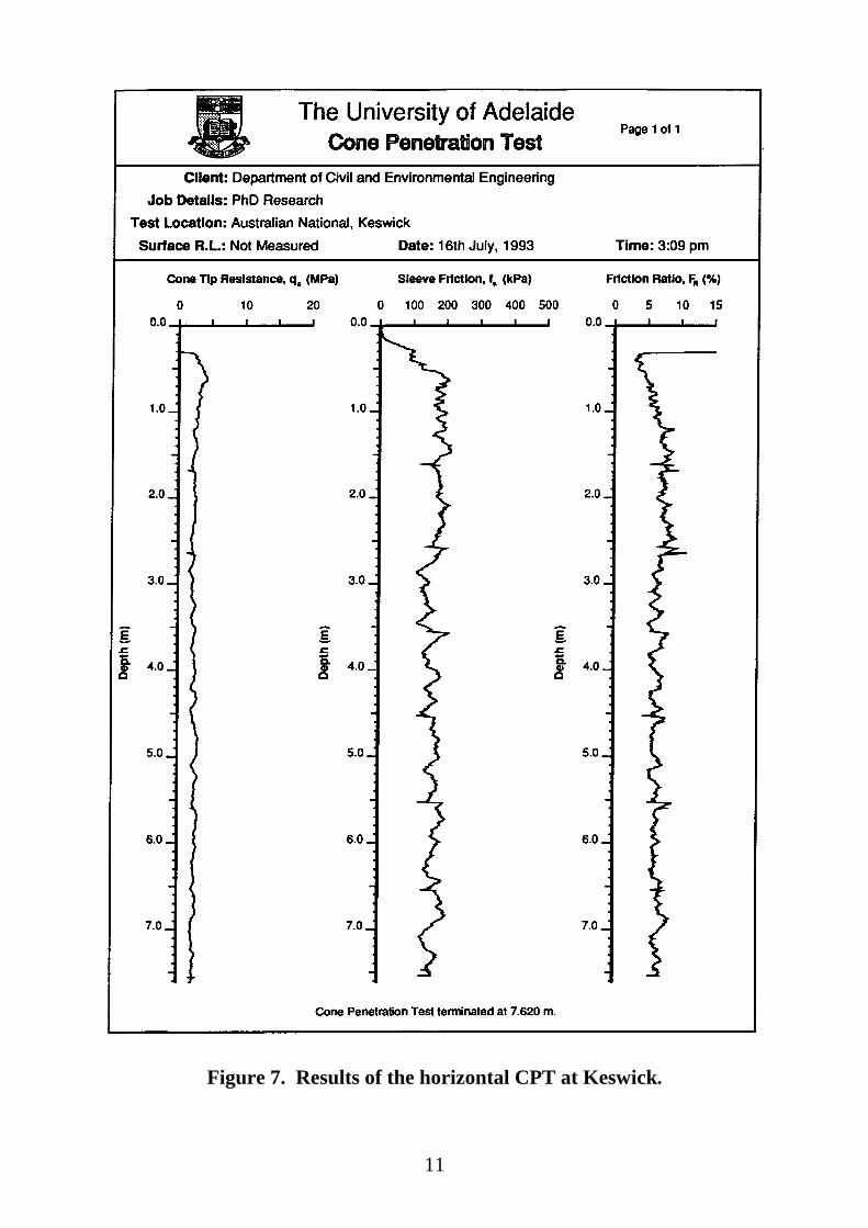
7.62 metres from the face of the embankment, as shown in Figure 3. The resultsof the CPT are shown in Figure 7.
Furthermore, due to complications caused by trailer movements, only two (2)undisturbed tube samples of Keswick Clay were obtained. However these wereunsuitable for triaxial testing purposes because of weathering and the presenceof plant roots in the region adjacent to the embankment face. Inspection ofthese samples, on the other hand, showed that the material tested by the CPTwas indeed Keswick Clay as originally anticipated.
6. SPATIAL VARIABILITY ANALYSES
To date the analysis of the spatial variability of geotechnical materials hasfocussed on two (2) mathematical techniques, namely, time series analysis, andgeostatistics. In order to provide a background to the analyses which follow in§7, these two techniques are treated briefly, below.
6.1 Time Series Analysis
A time series is a chronological sequence of observations of a particularvariable, usually, but not necessarily, at constant time intervals. When appliedto the study of the spatial variability of geotechnical materials, the time domainis replaced by the space, or distance, domain. In all other respects, the analysisprocedures and theory are identical. Unlike classical statistics, time seriesanalysis incorporates the observed behaviour that values at adjacent locationsare more related, than those at distant locations.
For time series analyses to be carried out the data must be stationary, that is, theprobabilistic laws which govern the series must be independent of the locationof the samples. Data are stationary if:
• the mean, µ, is constant with distance, that is, no trend, or drift, exists in thedata;
• the variance, σ2, is constant with distance, that is homoscedastic;• there are no seasonal variations; and,• there are no irregular fluctuations.
An important implication of the assumption of stationarity is that the statisticalproperties of the time series are unaffected by a shift of the spatial origin. Two
11
Figure 7. Results of the horizontal CPT at Keswick.
12
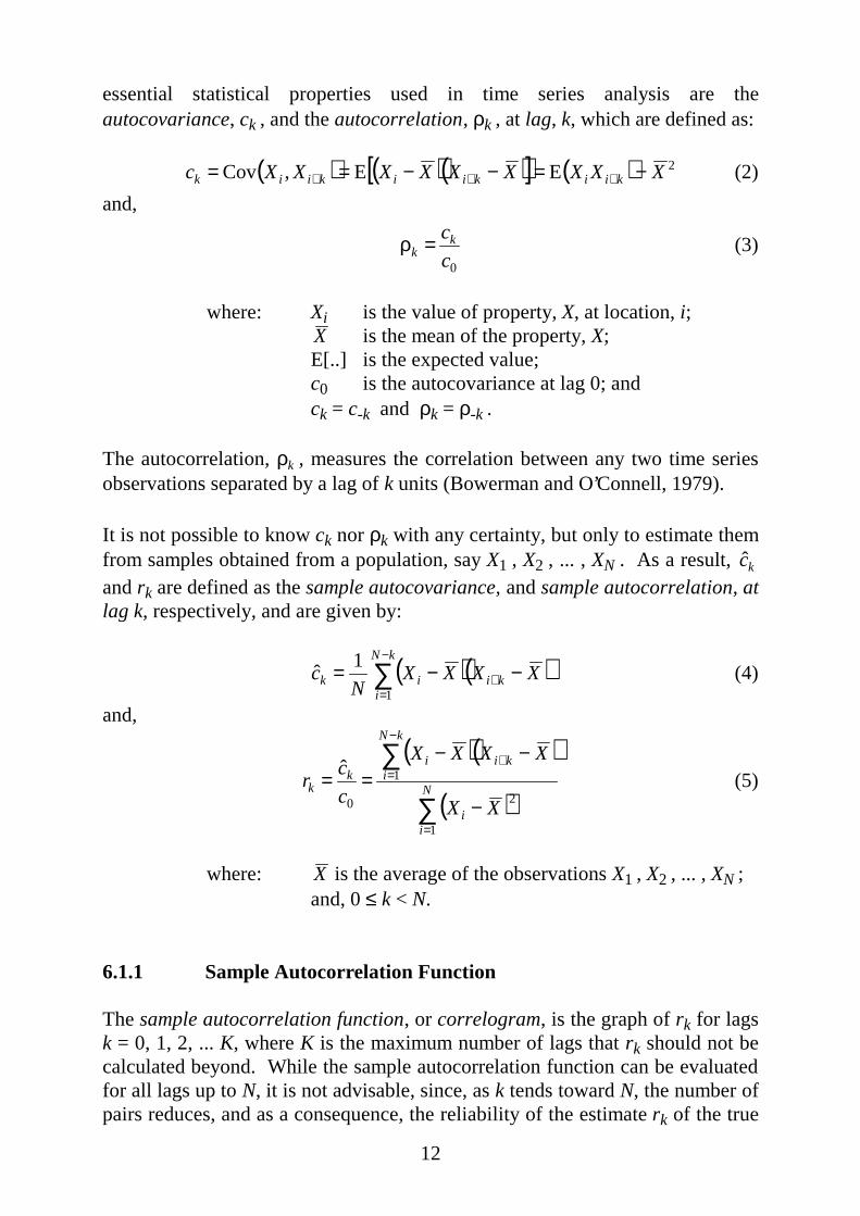
essential statistical properties used in time series analysis are theautocovariance, ck , and the autocorrelation, ρk , at lag, k, which are defined as:
( ) ( )( )[ ] ( ) 2EE,Cov XXXXXXXXXc kiikiikiik −=−−== +++ (2)
and,
0c
ckk =ρ (3)
where: Xi is the value of property, X, at location, i;X is the mean of the property, X;E[..] is the expected value;c0 is the autocovariance at lag 0; andck = c-k and ρk = ρ-k .
The autocorrelation, ρk , measures the correlation between any two time seriesobservations separated by a lag of k units (Bowerman and O’Connell, 1979).
It is not possible to know ck nor ρk with any certainty, but only to estimate themfrom samples obtained from a population, say X1 , X2 , ... , XN . As a result, kcand rk are defined as the sample autocovariance, and sample autocorrelation, atlag k, respectively, and are given by:
( )( )∑−
=+ −−=
kN
ikiik XXXX
Nc
1
1ˆ (4)
and,
( )( )
( )∑
∑
=
−
=+
−
−−== N
ii
kN
ikii
kk
XX
XXXX
c
cr
1
2
1
0
ˆ(5)
where: X is the average of the observations X1 , X2 , ... , XN ;and, 0 ≤ k < N.
6.1.1 Sample Autocorrelation Function
The sample autocorrelation function, or correlogram, is the graph of rk for lagsk = 0, 1, 2, ... K, where K is the maximum number of lags that rk should not becalculated beyond. While the sample autocorrelation function can be evaluatedfor all lags up to N, it is not advisable, since, as k tends toward N, the number ofpairs reduces, and as a consequence, the reliability of the estimate rk of the true

13
autocorrelation function, ρk , also decreases. Various authors have suggestedthe following values of K:
• KN=4
, (Box and Jenkins, 1970; Chatfield, 1975; Anderson, 1976);
• K = 12 for non-seasonal time series, and K = 4L for seasonal time series,where L is the number of data in a year: eg. L = 12 for monthly data, L = 4for quarterly data, (Bowerman and O’Connell, 1979);
• K N= +10, (Cryer, 1986);• 20 ≤ K ≤ 40, (Brockwell and Davis, 1987; Hyndman, 1990);
An example of a discrete sample autocorrelation function is shown in Figure 8.
-1
-0.8
-0.6
-0.4
-0.2
0
0.2
0.4
0.6
0.8
1
0
1 2 3 4 5 6 7 8 9 10 11 12 Lag, k
Figure 8. Example of a discrete sample autocorrelation function.
As one might expect, the accuracy of the sample autocorrelation function isdirectly related to the number of observations in the time series, N. Littleguidance is given to the minimum number of observations, though Box andJenkins (1970) and Anderson (1976) recommended that N be greater than 50.With particular reference to the spatial variability of soils, Lumb (1975)suggested that, for a full three-dimensional analysis, the minimum number oftest results needed to give reasonably precise estimates is of the order of 104,which is prohibitively large, even for a special research project. On the otherhand, Lumb (1975) recommended that the best that can be achieved in practiceis to study the one-dimensional variability, either vertically or laterally, using Nof the order of 20 to 100.

14
The autocorrelation function (ACF) is used widely throughout time seriesanalysis literature, and it enables the characteristics of the time series to bedetermined. For example, an ACF exhibiting slowly decaying values of rk withincreasing k, suggests long term dependence, such as that shown in Figure 8,whereas rapidly decaying values of rk suggest short term dependence (Chatfield,1975; Hyndman, 1990). A purely random time series, or white noise, ischaracterised by an ACF with the following properties:
≠=
=ρ0for 0
0for 1
k
kk (6)
Vanmarcke (1977a, 1983) suggested that the spatial variability of geotechnicalmaterials may be characterised stochastically by the use of three parameters, themean, µ, the standard deviation, σ, and the scale of fluctuation, δv . Vanmarckedefined the scale of fluctuation as the distance within which a soil property, v,shows relatively strong correlation, or persistence, from point-to-point. Inaddition, Vanmarcke suggested that the scale of fluctuation is closely related tothe average distance between intersections, or crossings, of v and µ - smallvalues of δv imply rapid fluctuations about the mean, whereas large valuessuggest a slowly varying property with respect to the average.
Vanmarcke (1983) proposed that δv may be evaluated by fitting a model ACF tothe sample ACF. Some standard, model ACFs, and their relationship to δv , areshown in TABLE 1.
TABLE 1. SCALES OF FLUCTUATION WITH RESPECT TOTHEORETICAL AUTOCORRELATION FUNCTIONS(After Vanmarcke, 1977a, 1983).
Model No. Autocorrelation Function Scale of Fluctuation, δv
1 ρhh ae= − 2a
2 ( )ρhh be= − 2
π b
3 ρhh ce
hc= +
− 1 4c

15
6.1.2 Cross-Covariance and the Cross-Correlation Function
Just as the ACF is used to measure dependencies by comparing a time serieswith itself at successive lags, it is also possible to compare two separate timeseries with each other to calculate positions of strong correlation. The toolsused to do this are: the cross-covariance, and the cross-correlation function(CCF). The cross-covariance coefficients between two time series,
NXXXXX , ,,, 321 K= , and NYYYYY , ,,, 321 K= , at lag k, ckXY, is given by (Box
and Jenkins, 1970):
( )( )[ ] K ,2 ,1 ,0 E =−−= + kYYXXc kiikXY(7)
and the cross-covariance between Y and X at lag k, ckYX, is:
( )( )[ ] K ,2 ,1 ,0 E =−−= + kXXYYc kiikYX(8)
where, in general, c ck kXY YX≠ . However, since:
( )( )[ ] ( )( )[ ]YXXY kkiiikik cXXYYYYXXc −−− =−−=−−= EE (9)
only ckXY need be calculated for k = 0, ± 1, ± 2, ± ... .
Since the time series, X and Y, may be expressed in different units, it is useful todefine the cross-correlation coefficient at lag k, ρkXY
, as:
K ,2 ,1 ,0 ±±±=σσ
=ρ kc
YX
kk
XY
XY(10)
where: σX standard deviation of X; andσY standard deviation of Y.
Again, only estimates can be made of ckXY and ρkXY
, and hence the sample
cross-covariance coefficient at lag k, XYkc , and the sample cross-correlation
coefficient at lag k, rkXY, are defined as:
( )( )
( )( )
=−−
=−−
=
∑
∑
+
=−
−
=+
K
K
,2- ,1- ,0 1
,2 ,1 ,0 1
ˆ
1
1
kXXXXN
kXXXXN
ckN
ikii
kN
ikii
kXY
(11)

16
K ,2 ,1 ,0 ˆ
±±±== kss
cr
YX
kk
XY
XY(12)
where: sX sample standard deviation of X = cXX0 ; and
sY sample standard deviation of Y = cYY0 .
Again, the accuracy of the sample cross-correlation function is directly relatedto the number of observations in the time series, N. As for the sample ACF,Box and Jenkins (1970) recommended that N be greater than 50.
6.2 Geostatistics
The mathematical technique, which is now universally known as geostatistics,was developed to assist in the estimation of changes in ore grade within a mine,and is largely a result of the work of D. G. Krige and G. Matheron (1965).Since its development in the 1960’s, geostatistics has been applied to manydisciplines including: groundwater hydrology and hydrogeology; surfacehydrology; earthquake engineering and seismology; pollution control;geochemical exploration; and geotechnical engineering. In fact, geostatisticscan be applied to any natural phenomena that are spatially or temporallyassociated (Journel and Huijbregts, 1978; Hohn, 1988).
Geostatistics is based on the regionalised variable, that is, one that can berepresented by random functions, rather than the classical approach which treatssamples as independent realisations of a random function. The regionalisedvariable has properties that are partly random and partly spatial and hascontinuity from point to point, but the changes are so complex that they cannotbe described by a tractable deterministic function (Davis, 1986).
One of the basic statistical measures of geostatistics is the semivariogram,which is used to express the rate of change of a regionalised variable along aspecific orientation. The semivariogram is treated below.
6.2.1 Semivariogram
The semivariogram is a measure of the degree of spatial dependence betweensamples along a specific orientation, and presents the degree of continuity of theproperty in question. The semivariogram, γh , is defined by Equation (13).

17
( )[ ]2E2
1ihih XX −=γ + (13)
where: Xi the value of the property, X, at location, i;Xi+h the value of the property, X, at location, i+h;h the displacement between the data pairs, andE[..] the expected value.
Thus, the semivariogram is defined as half the expected value, or mean, of thesquared difference between pairs of points, Xi and Xi+h , separated by adisplacement, h. The semivariogram is generally presented graphically; anexample is shown in Figure 9.
0
50
100
150
0 50 100
Displacement, h
Figure 9. Example of a semivariogram.
If the regionalised variable is stationary and normalised to have a mean of zeroand a variance of 1.0, the semivariogram is the mirror image of theautocorrelation function, as shown in Figure 10.
Even though a regionalised variable is spatially continuous, it is not possible toknow its value at all locations. Instead its values can only be determined fromsamples taken from a population. Thus, in practice, the semivariogram must beestimated from the available data, and is generally determined by therelationship shown in Equation (14).

18
0
10
20
30
40
50
60
70
80
-0.2
0
0.2
0.4
0.6
0.8
1
0 20 40 60 800 10 20 30 40 50 60 70 80
Autocorrelation
Semivariogram
Displacement, h
Figure 10. Relationship between semivariogram, γh , and autocorrelation,ρh , for a stationary regionalised variable. (After Davis, 1986)
( )∑=
+ −=γh
ii
N
ixhx
hh
YYN 1
2*
2
1(14)
where: γ h* the experimental semivariogram, that is, one based on the
sampled data set;
Yxithe value of the property, Y, at location, xi ;
Nh the number of data pairs separated by the displacement, h.
As the accuracy of γ h* is directly related to the number of data pairs, Nh
(Brooker, 1991), the experimental semivariogram is usually determined up tohalf of the total sampled extent (Journel and Huijbregts, 1978; Clark, 1979;Brooker, 1989). For example, if a CPT sounding was performed to a depth of5,000 mm, the semivariogram would be calculated for values of h from 0 to2,500 mm. The minimum number of pairs needed for a reliable estimate of γ h
*
is between 30 and 50 (Journel and Huijbregts, 1978; Brooker, 1989), with someauthors suggesting as many as 400 to 500 (Clark, 1980).
The strength of geostatistics is that it provides, through the semivariogram, aframework for the estimation of variables. In fact, it can be shown thatgeostatistics provides the best, linear, unbiased estimator (BLUE) (Journel andHuijbregts, 1978; Clark, 1979; Rendu, 1981). Whilst the experimentalsemivariogram is known only at discrete points, the estimation procedure,

19
known as kriging, requires the semivariogram values be known for all h. Thus,it is necessary to model the experimental semivariogram, γ h
* , as a continuous
function, γh . TABLE 2 and Figure 11 present a number of semivariogrammodels that are commonly used in the literature, the most widely applied ofthese being the spherical model.
With particular reference to the spherical model, three parameters are used:
Co is defined as the nugget effect and arises from the regionalisedvariable being so erratic over a short distance that thesemivariogram goes from zero to the level of the nugget in adistance less than the sampling interval. The nugget effect is dueto two factors (Journel and Huijbregts, 1978): (i) micro-variabilities of the mineralisation - since the structure of thesemicro-variabilities is not available at the scale at which the dataare measured; and (ii) measurement errors. It has been standardpractice in the treatment of the spatial variation of soils toattribute this nugget effect to measurement errors associated withthe testing method (Baecher, 1985; Wu and El-Jandali, 1985;Filippas et al., 1988). However, Li and White (1987) suggestedthat while some of the nugget effect can be attributed tomeasurement errors, the possibility of small scale random effectscannot be ignored in geotechnical properties;
TABLE 2. COMMONLY USED MODEL SEMIVARIOGRAMS.
Model Mathematical Function Remarks
Pure Nugget oh C=γ Co = Nugget
SphericalahCC
ahCa
h
a
hC
oh
oh
≥+=γ
≤+
−=γ
when
when 22
33
3
C + Co = Sill;
a = Range
Exponential ( ) oah
h CeC +−=γ −1
Gaussian ( ) oah
h CeC +−=γ − 22
1
Linear oh Ch +=γ p p = slope
Power oh Ch +=γ αp 0 < α < 2
de Wijsian oh Ch +α=γ )ln(3
NOTE: In addition, each of the models, above, obey γ0 = 0.

20
0
50
100
0 50 100
Spherical
Gaussian
Exponential
Displacement, h
0
50
100
0 50 100
Power
de Wijsian
Linear
Displacement, h
Figure 11. Commonly used model semivariograms with Co set to zero.
C + Co is known as the sill which measures half the maximum, onaverage, squared difference between data pairs;
a is defined as the range of influence, and is the distance at whichsamples become independent of one another. Data pairsseparated by distances up to a are correlated, but not beyond.
Clark (1979) described the process of fitting a model to an experimentalsemivariogram as essentially a trial-and-error approach, usually achieved byeye. Brooker (1991) suggested the following technique as a first approximationin finding the appropriate parameters for a spherical model:
• The experimental semivariogram and variance of the data be plotted;• The value of the sill, C + Co , is approximately equal to the variance of the
data;• A line is drawn with the slope of the semivariogram near the origin which
intersects the sill at two thirds the range, a;• This line intersects the ordinate at the value of the nugget effect, Co .
In addition, Brooker (1991) stated that the accuracy of the modelling processdepends on both the number of pairs in the calculation of the experimentalsemivariogram and the lag distance at which it is evaluated.
Journel and Huijbregts (1978) suggested that automatic fitting of models toexperimental semivariograms, such as least squares methods, should beavoided. This is because each estimator point, γ h
* , of an experimental
semivariogram is subject to an estimation error and fluctuation which is relatedto the number of data pairs associated with that point. Since the number of pairsvaries for each point, so too does the estimation error. The authors recommended

21
that the weighting applied to each estimated point, γ h* , should come from a
critical appraisal of the data, and from practical experience.
Similar to the autocorrelation function of random variables, the semivariogramrequires stationarity, that is, the semivariogram depends only on the separationdistance and not on the locality of the data pairs. The regionalised variable canbe regarded as consisting of two components: the residual and the drift. If adrift, or trend, exists in the data, which leads to non-stationarity, it must first beremoved. It has been shown by Davis (1986), that if the drift is subtracted fromthe regionalised variable, the residuals will themselves be a regionalisedvariable and will have local mean values of zero. In other words, the residualswill be stationary and the semivariogram can be evaluated.
6.3 SemiAuto
A Windows based program, SemiAuto, has been developed by the first authorto model the spatial variability of soils, and was used to analyse the horizontalCPT data, as will be discussed in §7. SemiAuto reads a CPT, or other, data fileand carries out the following:
• evaluates the basic statistics of the data;• enables data transformation (removal of the mean or trend function, in
addition to first-, and second-order differencing);• evaluates the undrained shear strength from the measured values of qc ;• plots the data and trend function (linear, quadratic, or cubic) with depth;• calculates and plots the semivariogram, cross-semivariogram, and auto-
correlation, partial autocorrelation, and cross-correlation functions;• allows standard models to be fitted to the autocorrelation function and the
semivariogram; and• enables transformed data and the calculated semivariograms and time series
functions to be saved to a text file for subsequent analysis and presentation.
SemiAuto was written using Visual Basic® Version 3.0 Professional Editionbecause of its Windows support, and its straightforward ability to utilise themany Windows features.

22
7. RESULTS
As discussed in §5, no undisturbed samples of the Keswick Clay were able to beobtained due to equipment inadequacies and externally imposed timeconstraints. As a result, it was not possible to determine the cone factor, Nk , ofthe clay, nor, as a consequence, its undrained shear strength. Do and Potter(1992) and van Holst Pellekaan and Cathro (1993) performed a number ofvertical CPTs, and obtained several undisturbed samples of Keswick Clay fromVictoria Square, located within the central business district of Adelaide. Theauthors carried out unconsolidated undrained (UU) triaxial tests on theundisturbed samples of Keswick Clay, and both found that Nk variedconsiderably (between 12.5 and 29.2) and inconsistently with depth. It isimperative in the study of spatial variability to eliminate as many sources oferror as possible so that the structure of the spatial variation can be identifiedand isolated from other sources of uncertainty. As the conversion of qcmeasurements to su , by means of Equation (1), will introduce further variabilityto the measured data, subsequent analyses of these data will be based on themeasured values of qc , rather than derived values of su .
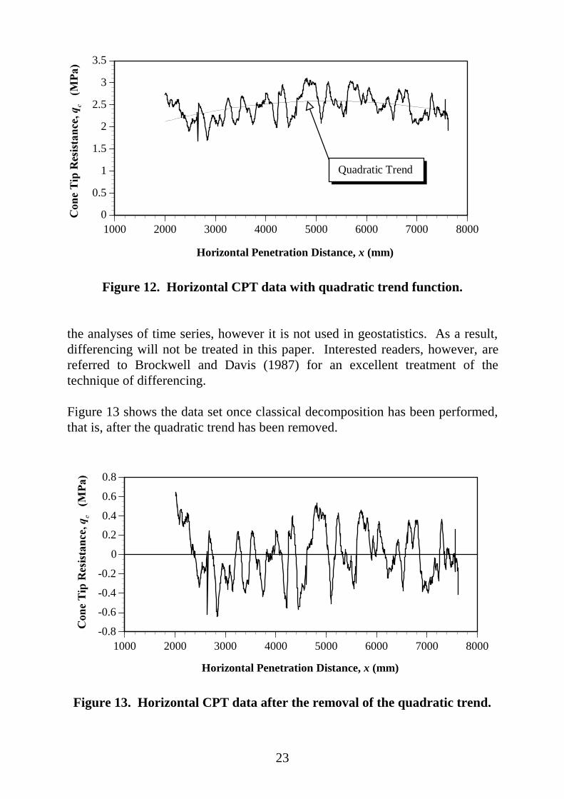
Figure 12 shows the measured values of qc plotted against the horizontalpenetration distance for the CPT conducted at the Keswick site. The first twometres of data have been removed from the data set as these measurements arelikely to have been influenced by weathering and movement adjacent to the faceof the embankment. In addition, Figure 12 shows a quadratic trend, indicatedby Equation (15), fitted to the data by the method of least-squares regression.
28-4 104.44104.661.37 xxqc−×−×+= (15)
where: qc is the cone tip resistance in MPa; andx is the horizontal distance of penetration in mm.
The statistics for the horizontal qc data set are: mean, µ = 2.46 MPa; standarddeviation, σ = 0.284 MPa2; coefficient of variation = 11.53%; skewness =0.106 MPa3; kurtosis = 2.38 MPa4, and the number of values, N, = 1106.
The presence of a quadratic trend function, as shown in Figure 12, suggests thatthe data set is non-stationary. Brockwell and Davis (1987) proposed twotechniques for transforming a non-stationary data set into a stationary one:classical decomposition and differencing. Classical decomposition involvesremoving the trend component by simply subtracting the trend function from thedata set, which is obtained by least-squares regression. Differencing, on theother hand, enables both the trend component, and a seasonal component, if oneexists, to be removed from the data. Differencing has been widely applied to
23
0
0.5
1
1.5
2
2.5
3
3.5
1000 2000 3000 4000 5000 6000 7000 8000
Horizontal Penetration Distance, x (mm)
Quadratic Trend
Figure 12. Horizontal CPT data with quadratic trend function.
the analyses of time series, however it is not used in geostatistics. As a result,differencing will not be treated in this paper. Interested readers, however, arereferred to Brockwell and Davis (1987) for an excellent treatment of thetechnique of differencing.
Figure 13 shows the data set once classical decomposition has been performed,that is, after the quadratic trend has been removed.
-0.8
-0.6
-0.4
-0.2
0
0.2
0.4
0.6
0.8
1000 2000 3000 4000 5000 6000 7000 800008000
Horizontal Penetration Distance, x (mm)
Figure 13. Horizontal CPT data after the removal of the quadratic trend.

24
7.1 Time Series Analyses
This sub-section details the results of time series analyses performed on the de-trended cone tip resistance data, shown in Figure 13. Figure 14 shows theresulting sample autocorrelation function (ACF) obtained by substituting thede-trended data into Equation (5). In addition, Figure 14 shows two of the threemodel ACFs given in TABLE 1, and suggested by Vanmarcke (1977a, 1983),fitted to the sample ACF by means of least-squares regression. The modelparameters are summarised in Figure 14 and TABLE 3.
[[[[[[[[[[[[[[[[[[[[[[[[[[[[[[[[[[[[[[[[[[[[[[[[[[[[[[[[[[[[[[[[[[[[[[[[[[[[[[[
[[[[[[[[[[[[[[[[[[[[[[[[[[[[[[[[[[[[[[[[[[[[[[[[[[[[[[[[[[[[[[[[[[[[[[[[[[[[[[[[[[[[[[[[[[[[[[[[[[[[[[[[[[[[[[[[[[[[[[[[[[[[[[[[[
[[[[[[[[[[[[[[[[[[[[[[[[[[[[[[[[[[[[[[[[[[[[[[[[[[[[[[[[[[[[[[[[[[[[[[[[[
-1
-0.8
-0.6
-0.4
-0.2
0
0.2
0.4
0.6
0.8
1
0
500 1000 1500
Horizontal Spacing, h (mm)
Model 1
Model 2Experimental acf[
Figure 14. Sample and model autocorrelation functions ofthe de-trended horizontal CPT data.
As can be seen from Figure 14 and TABLE 3 the model ACFs fit the sampleACF reasonably well, and the resulting scales of fluctuation are identical.
Another technique for determining the approximate distance over whichsamples show significant autocorrelation is to use Bartlett’s formula (Box andJenkins, 1970; Brockwell and Davis, 1987), as given in Equation (16).
NNrhh
296.1 when 0 ±≈±≤≈ρ (16)
where: N is the total number of samples.

25
TABLE 3. SUMMARY OF TIME SERIES ANALYSES.
Model No. Model ACF Parameters Scale of Fluctuation, δv
1 ahh e−=ρ a = 71 mm 142 mm
2 ( )2bhh e−=ρ b = 80 mm 142 mm
3
+=ρ −
c
he ch
h 1 c = 35.6 mm 142 mm
That is, the samples are considered to be autocorrelated when the sampleautocorrelation coefficient, rh , is less than N2± . Applying Bartlett’sformula to the de-trended data yields the limit as being equal to 0.060, whichoccurs at a lag of 28, or an horizontal distance of 140 mm. This result is almostidentical to the 142 mm obtained for δv .
7.2 Geostatistical Analyses
This sub-section details the results of geostatistical analyses performed on thede-trended cone tip resistance data, shown in Figure 13. Figure 15 shows theexperimental semivariogram obtained by substituting the de-trended data intoEquation (14). The number of pairs used in the determination of theexperimental semivariogram decreases linearly from 1095 at lag 1, to 544 at lag562. In addition, Figure 15 shows a spherical model semivariogram fitted to theexperimental semivariogram. The model is represented by the followingequation:
ahCC
ahCa
h
a
hC
Oh
Oh
≥+=γ
≤+
−=γ
when
when 22
33
3
(17)
where: C = 0.068 MPa2;a = 190 mm; andCO = 0 MPa2.
As can be seen from Figure 15, the spherical model fits the experimentalsemivariogram reasonably well, especially forvalues of h between 0 and therange, a. The range of 190 mm is comparable to the scale of fluctuation and theautocorrelation distance of 140 mm obtained in §7.1, though it is likely thateach of these parameters measures different spatial variability characteristics.

26
[[[[[[[[[[[[[[[[[[[[[[[[[[[[[[[[[[[[[[[[[[[[[[[[[[[[[[[[[[[[[
[[[[[[[[[[[[[[[[[[[[[[[[[[[[[[[[[[[[[[[[[[[[[[[[[[[[[[[[[
[[[[[[[[[[[[[[[[[[[[[[[[[[[[[[[[[[[[[[[[[[[[[[[[[[[[[[[[[[[[[[[[[[[[[[[[[[[[[[[[[[[[[[[[[[[[[[[[[[[[[[[[[[[[[[[[[[[[
[[[[[[[[[[[[[[[[[[[[[[[[[[[[[[[[[[[[[[[[[[[[[[[[[[[[[[[[[[
[[[[[[[[[[[[[[[[[[[[[[[[[[[[[[[[[[[[[[[[[[[[[[[[[[[[[[[[[[[[[[[[[[[[[[[[[[[[[[[[[[[[[[[[[[[[[[[[[[[[[[
[[[[[[[[[[[[[[[[[[[[[[[[[[[[[[[[[[[[[[[[[[[[[[[[[[[[[[[[[[[[[[[[[[[[[[[[[[[[[[[[[[[[[[[[[[[[[[[[[[[[[[[[[[[[[[[[[[[[[[[[[[
[[[[[[[[[[[[[[[[[[[[[[[[[[[[[[[[[[[[[[[[[[[[[[0.00
0.01
0.02
0.03
0.04
0.05
0.06
0.07
0.08
0.09
0.10
0 500 1000 1500 2000 2500 3000
[ Experimental Semivariogram
Spherical Model, a = 190 mm
Horizontal Spacing, h (mm)
Figure 15. Experimental and model semivariograms ofthe de-trended horizontal CPT data.
The correlation distance of approximately 200 mm, obtained for the KeswickClay using both time series analyses and geostatistics, is surprisingly lowconsidering that the clay appears, from a visual inspection, to be veryhomogeneous over many hundreds of metres. Few researchers have examinedthe lateral spatial variability of the undrained shear strength of clay soils,however, Vanmarcke (1977b) suggested that the horizontal correlation distancefor the undrained shear strength of a Canadian varved clay was 46 m, based onfield vane tests performed in a series of vertical boreholes. In addition, Tang(1979) suggested that the horizontal correlation distance for a North Sea claydeposit was 30 m, based on a small number of vertical CPTs drilled at lateralspacings of approximately 20 m. On the basis of the results presented in thisreport, one wonders whether the resulting correlation distance would have beenfar smaller if these researchers had performed a larger number of more closelyspaced tests.
7.3 Cross-Correlation Analyses
Several researchers and codes of practice (Standards Association of Australia,1977; American Society of Testing and Materials, 1986; Schmertmann, 1978;De Beer et al., 1988) suggest that when interpreting or presenting CPT results,attention shall be given to the fact that when measurements of qc and fs are

27
recorded, they do not correspond to the same depth because the cone tipresistance and friction sleeve load cells are physically separated by a knowndistance. In cones of standard dimensions (Standards Association of Australia,1977; American Society of Testing and Materials, 1986; De Beer et al., 1988)the distance from the tip of the cone to the centre of the friction sleeve isapproximately 75 mm. Schmertmann (1978) suggested that if attention is notgiven to this depth anomaly errors can result from the interpretation of CPTmeasurements, such as the calculation of the friction ratio, FR
( ( )= ×f qs c 100%). Generally, this is achieved by shifting the fs values back bythe shift distance, usually 75 mm. However, it is difficult to know the actualshift distance, as it is a complex problem which involves the extent of the zonesof soil which contribute to the measurements of qc and fs , and the distancebetween these zones.
The cross-correlation function provides a relatively simple, statistical techniquefor determining this shift distance. The measured values of qc and fs , shown inFigure 7, were substituted into Equations 11 and 12, and the resulting cross-correlation function is shown in Figure 16.
[[[[[[[[[[[[[[[[[[[[[[[[[[[[[[[[[[[[[[[[[[[[[[[[[[[[[[[[[[[[
[[[[[[[[[[[[[[[[[[[[[[[[[[[[[[[[[[[[[[[[[[[[[[[[[[[[[[[[[[[[[[
[[[[[[[[[[[[[[[[[[[[[[[[[[[[[[[[[[[[[[[[[[[[[[[[[[[[[[[[[[[[[[[[[[[[[[[[[[[[[[[[[[[
[[[[[[[[[[[[[[[[[[[[[[[[[[[[[[[[[[[[[[[[[[[[[[[[[[[[[[[[[[[[[[[[[[[
[[[[[[[[[[[[[[[[[[[[[[[[[[[[[[[[[[[[[[[[[[[[[[[[[[[[[[[[[[[[[[[[[[[[[[[[[[[[[[[[[[[[[[[[[[[[[[[[[[[[[[[[[[[[[[[[[[[[[[[[[[[[[[[[[[[[[[[[[[[[[[[[[[[[[[[[[[[[[[[[[[[[[[[[[[[[[[[[[[[[[[[[[[[[[[[[[[[[[
[[[[[[[[[[[[[[[[[[[[[[[[[[[[[[[[[[[[[[[[[[[[[[[[[[[[[[[[[[[[[[[[[[[[[[[[[[[[[[[[[[[[[[[
[[[[[[[
-1
-0.8
-0.6
-0.4
-0.2
0
0.2
0.4
0.6
0.8
1
-1500 -1000 -500
0500
1000 1500
Cross-Correlation Coefficient
Horizontal Spacing, h (mm)
Figure 16. Sample cross-correlation function of cone tip resistanceand sleeve friction data.
The maximum cross-correlation coefficient, of magnitude +0.607, occurs at alag of -24, or 120 mm, somewhat larger than the 75 mm physical separation ofthe two load cells.

28
7.4 Comparison of Results
Jaksa et al. (1993) reported the results of preliminary spatial variability analysesperformed on a subset of 201 CPTs each drilled vertically to a depth ofapproximately 5 metres. The tests were carried out in Keswick Clay, and asshown in Figure 17, were arranged in a 5 x 5 metre grid, and in a ‘cross’formation with each CPT being spaced at 1 metre centres.
5 m
50 m
50 m
5 m
1 m
1 m
0 1 2 3 4 5 6 7 8 9 10A
B
C
D
E
F
G
H
I
J
K
Tests examinedin this paper
Legend
Continuous core sample
3.2
2.65
1.3
2.57 1.0
1.3
2.25
2.25
1.0 Depth to top of Keswick Clay
Triaxial samples
Figure 17. Layout of cone penetration tests as reportedby Jaksa et al. (1993).

29
The authors carried out geostatistical analyses in both the vertical andhorizontal directions, and concluded that the range of influence, a, for thevertical direction varied between 600 mm and 1,750 mm, whereas, for thelateral variability of the Keswick Clay, the authors concluded that a was lessthan one metre, and as a result, the vertical CPT soundings should be spaced atintervals of less than one metre. The horizontal range of influence ofapproximately 200 mm, presented in §7.2, therefore, is in agreement with thatspecified by Jaksa et al. (1993).
Subsequent cross-correlation analyses performed on the vertical CPT data ofJaksa et al. (1993) indicate that the sleeve friction shift distance varies between75 mm and 165 mm, with an average of 115 mm, which agrees well with the120 mm obtained in the previous section.
8. CONCLUSIONS
This paper has examined the application of a cone penetration test (CPT) carriedout in the horizontal direction to determine the lateral spatial variability of astiff, overconsolidated clay, known as the Keswick Clay. In summary, thefollowing conclusions are made:
1. The horizontal CPT is an extremely useful tool for enabling the lateralspatial variability to be quantified. The technique, however, is limited tospecial site conditions, requires specialised equipment, and can besomewhat expensive.
2. The techniques of time series analyses and geostatistics are useful fordetermining spatial variability characteristics, and provide similar results.They do, however, require large amounts of data. The CPT is able toprovide the quantity of data necessary for these analytical techniques, in areliable, accurate, efficient, and economic manner.
3. Since the lateral restraining system, detailed in §5, allowed the trailer torotate slightly during sampling, thereby enabling only a few undisturbedsamples to be taken, modifications to the system are needed. It isexpected that adequate lateral restraint of the trailer may be provided byrigidly connecting the chains to the 100UC piers, rather than the chainsbeing simply wrapped around the piers.
4. It has been found that the horizontal distance over which measurementsof the cone tip resistance, and hence the undrained shear strength, of theKeswick Clay are correlated, is approximately 200 mm. This result is inagreement with the conclusions made by Jaksa et al. (1993). In addition,

30
this low value of correlation distance may question the results publishedby others (eg. Vanmarcke, 1977b; Tang, 1979) who found correlationdistances much larger than 200 mm from discrete samples obtained fromrelatively large lateral spacings.
5. Cross-correlation analyses performed on the cone tip resistance andsleeve friction measurements indicate that the sleeve friction valuesshould be shifted back by a distance of approximately 120 mm.
6. Since the Keswick Clay has properties remarkably similar to those of thewell-documented London Clay, it is possible that the conclusionssummarised above may be extrapolated to other similar soils.
9. REFERENCES
Anderson, O. D. (1976). Time Series Analysis and Forecasting: The Box-Jenkins Approach, Butterworths, London, 182 p.
American Society for Testing and Materials (1986). Standard Method forDeep, Quasi-Static, Cone and Friction-Cone Penetration Tests of Soil (D3441).Annual Book of Standards, Vol. 04.08, ASTM, Philadelphia, pp. 552-559.
Baecher, G. B. (1985). Geotechnical Error Analysis. Transportation ResearchRecord, No. 1105, pp. 23-31.
Bergado, D. T., Alfaro, M. C., Patron Jr., B. C. and Chirapuntu, S. (1991).Reliability Based Analysis of Embankment Failures on Soft Ground. Proc. of6th Int. Symp. on Landslides, Vol. 1, Christchurch, Feb., 1992, A. A. Balkema,Rotterdam, pp. 321-328.
Bowerman, B. L. and O’Connell, R. T. (1979). Forecasting and Time Series,Duxbury Press, Massachusetts, 481 p.
Box, G. E. P. and Jenkins, G. M. (1970). Time Series Analysis Forecastingand Control, Holden-Day, San Fransisco, 553 p.
Brockwell, P. J. and Davis, R. A. (1987). Time Series: Theory and Methods,Springer-Verlag, New York, 519 p.
Brooker, P. I. (1989). Basic Geostatistical Concepts. In Workshop Notes ofAust. Workshop on Geostatistics in Water Resources, Vol. 1, Centre forGroundwater Studies, Adelaide, November.

31
Brooker, P. I. (1991). A Geostatistical Primer, World Scientific, Singapore,95 p.
Chatfield, C. (1975). The Analysis of Time Series: Theory and Practice,Chapman and Hall, London, 263 p.
Chen, Y.-J. and Kulhawy, F. H. (1993). Undrained StrengthInterrelationships Among CIUC, UU, and UC Tests. J. Geotech. Engg. Div.,ASCE, Vol. 119, No. 11, pp. 1732-1750.
Clark, I. (1979). Practical Geostatistics, Applied Science Publishers, London,129 p.
Clark, I. (1980). The Semivariogram. Chapters 2 and 3 of Geostatistics,McGraw-Hill Inc., New York, pp. 17-40.
Cox, J. B. (1970). A Review of the Geotechnical Characteristics of the Soils inthe Adelaide City Area. Symp. on Soils and Earth Structures in Arid Climates,Adelaide, Inst. Eng., Aust. and Aust. Geomech. Soc., May, 1970, pp. 72-86.
Cryer, J. D. (1986). Time Series Analysis, Duxbury Press, Boston, 286 p.
Davis, J. C. (1986). Statistics and Data Analysis in Geology, 2nd ed., JohnWiley and Sons, New York, 646 p.
De Beer, E. E., Goelen, E., Heynen, W. J. and Joustra, K. (1988). ConePenetration Test (CPT): International Reference Test Procedure. In PenetrationTesting, Proc. of the First Int. Symposium on Penetration Testing, de Ruiter, J.(ed.), Orlando, Florida, A. A. Balkema, Rotterdam, pp. 27-51.
Do, H. P. and Potter, S. M. (1992). Cone Factor Investigation for KeswickClay. Student Project Report, Dept. Civil and Environmental Engg., Uni. ofAdelaide, 66 p.
Filippas, O. B., Kulhawy, F. H. and Grigoriu, M. D. (1988). Evaluation ofUncertainties in the In-Situ Measurement of Soil Properties. Report EL-5507,Vol. 3, Electric Power Research Institute, Palo Alto, Oct. 1988.
Germaine, J. T. and Ladd, C. C. (1988). Triaxial Testing of SaturatedCohesive Soils. In Advanced Triaxial Testing of Soil and Rock, ASTM STP 977,Donaghe, R. T., Chaney, R. C. and Silver, M. L. (eds.), American Society forTesting Materials, Philadelphia, pp. 421-459.

32
Hohn, M. E. (1988). Geostatistics and Petroleum Geology, Van NostrandReinhold, New York, 264 p.
Hyndman, R. J. (1990). PEST - A Program for Time Series Analysis,Statistical Consulting Centre, University of Melbourne, 53 p.
Jaksa, M. B., Kaggwa, W. S. and Brooker, P. I. (1993). GeostatisticalModelling of the Undrained Shear Strength of a Stiff, Overconsolidated, Clay.Proc. of Conf. of Probabilistic Methods in Geotechnical Engineering, Canberra,A. A. Balkema, Rotterdam, pp. 185-194.
Jaksa, M. B. and Kaggwa, W. S. (1994). A Micro-Computer Based DataAcquisition System for the Cone Penetration Test. Research Report No. R 116,Dept. Civil & Environmental Engg., University of Adelaide, 31 p.
Jamiolkowski, M., Ghionna, V. N., Lancellotta, R. and Pasqualini, E.(1988). New Correlations of Penetration Tests for Design Practice. InPenetration Testing 1988, Proc. of 1st Int. Symp. on Penetration Testing,Orlando, Florida, Vol. 1, de Ruiter, J. (ed.), A. A. Balkema, Rotterdam, pp. 263-296.
Journel, A. G. and Huijbregts, Ch. J. (1978). Mining Geostatistics,Academic Press, London, 600 p.
Kulatilake, P. H. S. W. and Miller, K. M. (1987). A Scheme for Estimatingthe Spatial Variation of Soil Properties in Three Dimensions. Proc. 5th Int.Conf. Statistics and Probability in Soil and Struct. Eng., Vancouver, pp. 669-677.
Ladd, C. C., Foott, R., Ishihara, K., Schlosser, F. and Poulos, H. G. (1977).Stress-Deformation and Strength Characteristics. Proc. 9th Int. Conf. on SoilMech. and Foundation Engg., Vol. 2, Tokyo, pp. 421-494.
Li, K. S. and White, W. (1987). Probabilistic Characterization of Soil Profiles.Research Report, Dept. Civil Engg., Australian Defence Force Academy,Canberra, Australia.
Lumb, P. (1966). The Variability of Natural Soils. Can. Geotech. J., Vol. 3,pp. 74-97.
Lumb, P. (1975). Spatial Variability of Soil Properties. Proc. 2nd Int. Conf.Statistics and Probability in Soil and Struct. Eng., Auchen, pp. 397-421.

33
Matheron, G. (1965). Les Variables Regionalisees et leur Estimation. Massonet Cie, Paris, 212 p.
Orchant, C. J., Kulhawy, F. H. and Trautmann, C. H. (1988). CriticalEvaluation of In-Situ Test Methods and their Variability. Report EL-5507,Vol. 2, Electric Power Research Institute, Palo Alto, Oct. 1988.
Rendu, J.-M. (1981). An Introduction to Geostatistical Methods of MineralExploration, 2nd ed., South African Inst. Mining and Metallurgy, Johannesburg,84 p.
Schmertmann, J. H. (1978). Guidelines for Cone Penetration Test -Performance and Design. Report No. FHWA-TS-78-209, U.S. Dept.Transportation, Federal Highway Administration, Washington, 145 p.
Selby, J. and Lindsay, J. M. (1982). Engineering Geology of the AdelaideCity Area. Dept. Mines and Energy Bulletin 51, Adelaide, 94 p.
Sheard, M. J. and Bowman, G. M. (1987). Definition of Keswick Clay:Adelaide/Golden Grove Embayment, Para and Eden Blocks, South Australia.Q. geol. Notes, geol. Surv. S. Aust., 103, pp. 4-9.
Standards Association of Australia (1977). Methods for Testing Soils forEngineering Purposes, AS 1289, Sydney.
Sutcliffe, G. and Waterton, C. (1983). Quasi-Static Penetration Testing. InIn-Situ Testing for Geotechnical Investigations, Ervin, M. C. (ed.), A. A.Balkema, Rotterdam, pp. 33-48.
Tang, W. H. (1979). Probabilistic Evaluation of Penetration Resistances. J.Geotech. Engg. Div., ASCE, Vol. 105, No. GT10, pp. 1173-1191.
Van Holst Pellekaan, D. and Cathro, J. (1993). Investigating the Propertiesof Keswick Clay Using the Cone Penetration Test. Student Project Report,Department of Civil and Environmental Engg., Uni. of Adelaide, 163 p.
Vanmarcke, E. H. (1977a). Probabilistic Modeling of Soil Profiles. J.Geotech. Engg. Div., ASCE, Vol. 103, No. GT11, pp. 1227-1246.
Vanmarcke, E. H. (1977b). Reliability of Earth Slopes. J. Geotech. Engg.Div., ASCE, Vol. 103, No. GT11, pp. 1247-1265.
Vanmarcke, E. H. (1983). Random Fields: Analysis and Synthesis, M.I.T.Press, Cambridge, Mass., 382 p.

34
Wroth, C. P. (1984). The Interpretation of In Situ Soil Tests. Géotechnique,Vol. 34, No. 4, pp. 449-489.
Wu, T. H. and El-Jandali, A. (1985). Use of Time Series in GeotechnicalData Analysis, Geotech. Testing Journal, GTJODJ, Vol. 8, No. 4, pp. 151-158.