Embed Size (px)
Citation preview
Modelling the potential role of control strategies onEbola virus disease dynamics
by
Sylvie Diane Djiomba Njankou
Thesis presented in partial fulfilment of the requirements for thedegree of Master of Science in Mathematics in the Faculty of Science
at Stellenbosch University
Department of Mathematical Sciences,University of Stellenbosch,
Private Bag X1, Matieland 7602, South Africa.
Supervisor: Prof. Farai Nyabadza
December 2015
DeclarationBy submitting this thesis electronically, I declare that the entirety of the work containedtherein is my own, original work, that I am the sole author thereof (save to the extentexplicitly otherwise stated), that reproduction and publication thereof by StellenboschUniversity will not infringe any third party rights and that I have not previously in itsentirety or in part submitted it for obtaining any qualification.
Signature: . . . . . . . . . . . . . . . . . . . . . . . . . . . . . . . . .Sylvie Diane Djiomba Njankou
October 20, 2015Date: . . . . . . . . . . . . . . . . . . . . . . . . . . . . . . . . . . . . .
Copyright © 2015 Stellenbosch UniversityAll rights reserved.
i
Stellenbosch University https://scholar.sun.ac.za
Abstract
Modelling the potential role of control strategies on Ebola virus diseasedynamics
Sylvie Diane Djiomba Njankou
Department of Mathematical Sciences,University of Stellenbosch,
Private Bag X1, Matieland 7602, South Africa.
Thesis: MSc. (Mathematical Biology)
December 2015
The most deadly Ebola disease epidemic ever was still ongoing as of June 2015 in WestAfrica. It started in Guinea, where the first cases were recorded in March 2014. Controlstrategies, aiming at stopping the transmission chain of Ebola disease were publicisedthrough national and international media and were successful in Liberia. Using two dif-ferent approaches, the dynamics of Ebola disease is described in this thesis. First, a sixcompartments mathematical model is formulated to investigate the role of media cam-paigns on Ebola transmission. The model includes tweets or messages sent by individu-als with different disease status through the media. The media campaigns reproductionnumber is computed and used to investigate the stability of the disease free steady state.The presence of a backward bifurcation as well as a forward bifurcation are shown to-gether with the existence and local stability of the endemic equilibrium. We concludedthrough numerical simulations, that messages sent through media have a time limitedbeneficial effect on the reduction of Ebola cases and media campaigns must be spacedout in order to be more efficacious. Second, we use a seven compartments model todescribe the evolution of the disease in the population when educational campaigns, ac-tive case-finding and pharmaceutical interventions are implemented as controls againstthe disease. We prove the existence of an optimal control set and analyse the necessaryand sufficient conditions, optimality and transversality conditions. Using data from
ii
Stellenbosch University https://scholar.sun.ac.za

iii Abstract
affected countries, we conclude using numerical analysis that containing an Ebola out-break needs early and long term implementation of the joint control strategies.
Stellenbosch University https://scholar.sun.ac.za
Opsomming
Modellering van die potensiële rol van beheerstrategieë in dieEbolavirus-siektedinamika
(Modelling the potential role of control strategies on Ebola virus disease dynamics )
Sylvie Diane Djiomba Njankou
Departement Wiskundige Wetenskappe,Universiteit van Stellenbosch,
Privaatsak X1, Matieland 7602, Suid Afrika.
Tesis: MSc. (Wiskunde)
Desember 2015
In Junie 2015 was die dodelikste Ebola-epidemie ooit steeds voortslepend in Wes-Afrika.Dit het in Guinee uitgebreek, waar die eerste gevalle in Maart 2014 opgeteken is. Be-heerstrategieë daarop gemik om die oordragsketting van Ebola te stop is deur die na-sionale en internasionale media gepubliseer en was suksesvol in Liberië. In hierdietesis word die dinamika van Ebola aan die hand van twee verskillende benaderingsbeskryf. Eerstens is ’n sesvak- wiskundige model geformuleer om die rol van media-veldtogte in Ebola-oordrag te ondersoek. Die model sluit twiets of boodskappe ge-stuur deur individue met wisselende siektestatus deur die media in. Die mediaveldtog-weergawenommer is bereken en gebruik om die stabiliteit van die siektevry - ewewigs-toestand te bespreek. Die teenwoordigheid van ’n terugwaartse bifurkasie asook ’nvoorwaartse bifurkasie is getoon, tesame met die voorkoms en plaaslike stabiliteit vandie endemie-ewewig. Ons gevolgtrekking deur middel van numeriese simulasies is datboodskappe wat deur die media gestuur is ’n tydsbeperkte voordelige uitwerking opdie vermindering van Ebola-gevalle het en dat mediaveldtogte gespasieer moet wordom meer doeltreffend te wees. Tweedens is ’n sewevak-model gebruik om die evolusievan die siekte onder die bevolking te beskryf as opvoedkundige veldtogte, aktiewe ge-valopsporing en farmaseutiese intervensies as beheermaatreëls teen die siekte geïmple-
iv
Stellenbosch University https://scholar.sun.ac.za

v Abstract
menteer word. Die studie bewys die bestaan van ’n optimale beheerstel en ontleed dienodige en doeltreffende toestande, optimaliteit en transversaliteitsvoorwaardes. Metbehulp van data van lande wat deur die siekte geraak is, is die bevinding ná numerieseanalise dat vroegtydige en langtermyn-implementering van die gesamentlike beheer-strategieë nodig is om die uitbreek van Ebola te beheer.
Stellenbosch University https://scholar.sun.ac.za
Acknowledgements
I would like to thank God for giving me the strength and keeping me safe throughoutmy studies.I am grateful to Stellenbosch University for providing the resources that allowed me tocomplete this study.I would also like to thank my supervisor, Professor Farai Nyabadza for his guidance.I am grateful to my family, especially my parents and friends for supporting and moti-vating me during my research.Particular thanks to my blessed daughter Nganso Ngoma Diolvie for being strong in myabsence.This research project has benefited from the intellectual and material contribution of theOrganization for Women in Science for the Developing World (OWSD) and the SwedishInternational Development Cooperation Agency (SIDA).
vi
Stellenbosch University https://scholar.sun.ac.za

Dedications
To my lovely daughter Diolvie
vii
Stellenbosch University https://scholar.sun.ac.za
Publications
The following publications which are attached at the end of the list of references are theexpected publications that would arise from the thesis.
1. Modelling the potential role of media campaigns on Ebola transmission dynamics.Publication to be submitted.
2. An optimal control for Ebola virus disease. Submitted to the Journal of BiologicalSystems. Publication in review.
viii
Stellenbosch University https://scholar.sun.ac.za
Contents
Declaration i
Abstract ii
Opsomming iv
List of Figures xi
List of Tables xiii
1 Introduction 11.1 Ebola: the virus and the disease . . . . . . . . . . . . . . . . . . . . . . . . . 11.2 Ebola control strategies . . . . . . . . . . . . . . . . . . . . . . . . . . . . . . 3
1.2.1 Vaccines and treatments against Ebola . . . . . . . . . . . . . . . . . 31.2.2 Non pharmaceutical interventions against Ebola . . . . . . . . . . . 31.2.3 Media and communications on Ebola . . . . . . . . . . . . . . . . . 5
1.3 Motivation . . . . . . . . . . . . . . . . . . . . . . . . . . . . . . . . . . . . . 51.4 Objectives . . . . . . . . . . . . . . . . . . . . . . . . . . . . . . . . . . . . . 61.5 Significance of the study . . . . . . . . . . . . . . . . . . . . . . . . . . . . . 71.6 Overview of the thesis . . . . . . . . . . . . . . . . . . . . . . . . . . . . . . 7
2 Literature review 92.1 Media campaigns models . . . . . . . . . . . . . . . . . . . . . . . . . . . . 92.2 Optimal control models . . . . . . . . . . . . . . . . . . . . . . . . . . . . . 112.3 Ebola disease models . . . . . . . . . . . . . . . . . . . . . . . . . . . . . . . 13
3 Impact of media campaigns on Ebola transmission 163.1 Introduction . . . . . . . . . . . . . . . . . . . . . . . . . . . . . . . . . . . . 163.2 Model formulation . . . . . . . . . . . . . . . . . . . . . . . . . . . . . . . . 17
ix
Stellenbosch University https://scholar.sun.ac.za
Contents x
3.2.1 Model equations . . . . . . . . . . . . . . . . . . . . . . . . . . . . . 203.3 Model properties and analysis . . . . . . . . . . . . . . . . . . . . . . . . . . 20
3.3.1 Existence and uniqueness of solutions . . . . . . . . . . . . . . . . . 203.3.2 Positivity of solutions . . . . . . . . . . . . . . . . . . . . . . . . . . 213.3.3 Steady states analysis . . . . . . . . . . . . . . . . . . . . . . . . . . 223.3.4 The disease free equilibrium and RM . . . . . . . . . . . . . . . . . . 223.3.5 Existence and stability of the endemic equilibrium . . . . . . . . . . 25
3.4 Local stability of endemic equilibrium . . . . . . . . . . . . . . . . . . . . . 303.4.1 Bifurcation analysis . . . . . . . . . . . . . . . . . . . . . . . . . . . . 34
3.5 Numerical simulations . . . . . . . . . . . . . . . . . . . . . . . . . . . . . . 363.5.1 Parameters estimation . . . . . . . . . . . . . . . . . . . . . . . . . . 373.5.2 Simulations results and interpretation . . . . . . . . . . . . . . . . . 393.5.3 Model validation . . . . . . . . . . . . . . . . . . . . . . . . . . . . . 44
3.6 Conclusion . . . . . . . . . . . . . . . . . . . . . . . . . . . . . . . . . . . . . 48
4 An optimal control model for Ebola virus disease 494.1 Introduction . . . . . . . . . . . . . . . . . . . . . . . . . . . . . . . . . . . . 494.2 Model formulation . . . . . . . . . . . . . . . . . . . . . . . . . . . . . . . . 49
4.2.1 Model equations . . . . . . . . . . . . . . . . . . . . . . . . . . . . . 514.3 Definition and existence of an optimal control . . . . . . . . . . . . . . . . 52
4.3.1 Definition of an optimal control . . . . . . . . . . . . . . . . . . . . . 524.3.2 Invariance and positivity of solutions . . . . . . . . . . . . . . . . . 534.3.3 Existence of an optimal control . . . . . . . . . . . . . . . . . . . . . 55
4.4 Analysis of optimal control . . . . . . . . . . . . . . . . . . . . . . . . . . . 574.5 Numerical simulations and results . . . . . . . . . . . . . . . . . . . . . . . 60
5 General conclusion 67
Appendix i
List of references i
Stellenbosch University https://scholar.sun.ac.za
List of Figures
3.1 Flow diagram for EVD . . . . . . . . . . . . . . . . . . . . . . . . . . . . . . . . 193.2 Forward bifurcation for RM = 1.55 . . . . . . . . . . . . . . . . . . . . . . . . . 353.3 Backward bifurcation for RM = 0.92 . . . . . . . . . . . . . . . . . . . . . . . . 353.4 Time series variation of the force of infection for Rc
M = 0.72 with Λ = 0.8,µ = 0.0643, β ε [0.05, 0.07111, 0.8] , c = 2.9, σ = 0.0249, γ = 0.45, p = 0.6559,θ = 0.4640, δ1 = 0.123, δ2 = 0.603, ω = 0.99, α1 = 0.00034, α2 = 0.0000649,α3 = 0.0000212, α4 = 0.0000453, α5 = 0.00002. . . . . . . . . . . . . . . . . . . . 36
3.5 Population size at DFE for Λ = 9, µ = 0.01012, β = 0.19999567, c = 13, σ =
0.525, γ = 0.23511, p = 0.17, θ = 0.12, δ1 = 0.513, δ2 = 0.13, ω = 0.93, α1 =
2× 10⁻⁴, α2 = 2× 10⁻⁶, α3 = 5× 10⁻⁶, α4 = 8× 10⁻⁶, α5 = 9.9× 10⁻⁶, RM = 0.356.. . . . . . . . . . . . . . . . . . . . . . . . . . . . . . . . . . . . . . . . . . . . . 39
3.6 Population size at EE for Λ = 9, µ = 0.01012, β = 0.8, c = 15, σ = 0.525, γ =
0.09, p = 0.17, θ = 0.12, δ1 = 0.513, δ2 = 0.13, ω = 0.93, α1 = 2× 10⁻⁴, α2 =
2× 10⁻⁶, α3 = 5× 10⁻⁶, α4 = 8× 10⁻⁶, α5 = 9.9× 10⁻⁶, RM = 1.546. . . . . . . 403.7 Graph of α1 variations . . . . . . . . . . . . . . . . . . . . . . . . . . . . . . . . 413.8 Graph of α2 variations . . . . . . . . . . . . . . . . . . . . . . . . . . . . . . . . 413.9 Graph of α3 variations . . . . . . . . . . . . . . . . . . . . . . . . . . . . . . . . 423.10 Graph of α4 variations . . . . . . . . . . . . . . . . . . . . . . . . . . . . . . . . 423.11 Graph of α5 variations . . . . . . . . . . . . . . . . . . . . . . . . . . . . . . . . 433.12 Graph of ω variations . . . . . . . . . . . . . . . . . . . . . . . . . . . . . . . . 433.13 Cumulative number of suspected, probable and confirmed Ebola cases in
Guinea (1 term = 3 months). . . . . . . . . . . . . . . . . . . . . . . . . . . . . . 453.14 Curve fitting of the total number of Ebola cases in Guinea. The estimated
parameters values are: Λ = 0.8, µ = 0.0643, β = 0.3, σ = 0.0249, γ =
0.1075, p = 0.6559, θ = 0.4640, δ1 = 0.1231, δ2 = 0.0603, c = 1.57, ω =
0.99, α1 = 34× 10−6, α2 = 0.0643, α3 = 0.0212, α4 = 0.0453, α5 = 2× 10⁻¹⁰, RM =
2.036. . . . . . . . . . . . . . . . . . . . . . . . . . . . . . . . . . . . . . . . . . . 46
xi
Stellenbosch University https://scholar.sun.ac.za
List of figures xii
3.15 Reproduction number contour plot . . . . . . . . . . . . . . . . . . . . . . . . . 47
4.1 Flow diagram describing EVD dynamics. . . . . . . . . . . . . . . . . . . . . . 514.2 Dynamics of infected cases with and without control strategies for α1 =
0.1, α2 = 0.3, α3 = 0.2. . . . . . . . . . . . . . . . . . . . . . . . . . . . . . . . . 624.3 Graphical representations of control strategies for α1 = 100, α2 = 300, α3 = 200 634.4 Graphical representations of control strategies for α1 = 0.1, α2 = 0.3, α3 = 0.2 644.5 Aspects of optimal control with variations of the transmission rate . . . . . . 654.6 Aspects of optimal control with variations of the size of the total population . 65
Stellenbosch University https://scholar.sun.ac.za
List of Tables
3.1 Roots signs. . . . . . . . . . . . . . . . . . . . . . . . . . . . . . . . . . . . . . . 273.2 Model (3.2.1)-(3.2.6) parameters values . . . . . . . . . . . . . . . . . . . . . . . 38
4.1 Parameters values . . . . . . . . . . . . . . . . . . . . . . . . . . . . . . . . . . . 61
xiii
Stellenbosch University https://scholar.sun.ac.za
Chapter 1
Introduction
1.1 Ebola: the virus and the disease
Ebola is the name of a small river in the North West of the Democratic Republic ofCongo (DRC) where the Ebola virus was first identified in humans in 1976 [13]. Ebolavirus belongs to the family of Filoviruses, characterised by filamentous particles. Itsparticles have a uniform diameter of 80 nm with length up to 14000 nm [13]. As oth-ers Filoviruses, it is enveloped, non segmented, negative-stranded RNA with varyingmorphology. The production of a soluble glycoprotein, also secreted from infectedcells, makes it different from the other Mononegavirales [13]. There are five differentstrains of Ebola virus which have caused several outbreaks mainly on the African conti-nent namely Zaire ebolavirus, Sudan ebolavirus, Cote d’Ivoire ebolavirus, Bundibugyoebolavirus (Uganda) and Reston ebolavirus which has not yet caused disease in humans[13, 30]. The Zaire Ebola virus species caused the first outbreak in 1976, the outbreaksin Gabon, Republic of Congo, DRC and the actual 2014 outbreak in West Africa [13].This first strain is the most dangerous one, with a case fatality rate of 60− 90% [13, 30].In 1976, the Southern Sudan was affected by the Sudan Ebola virus strain whose casefatality rate was 40− 60% [13, 30]. In 1994 the third species was discovered, the Coted’Ivoire Ebola virus, which has only infected one individual up to now [13]. The fourthAfrican Ebola virus strain is the Bundibugyo species found in Equatorial Africa. TheReston Ebola virus species is the last one, found in Philippines for the first time in 1989and has not been identified in humans, but its emergence in pigs raised important con-cerns for public health, agricultural and food safety sectors in Philippines [13].
Ebola virus is transmitted to humans by animals. Rodents and bats have always beenconsidered as potential Ebola virus reservoirs [13, 30]. Transmission of the virus into
1
Stellenbosch University https://scholar.sun.ac.za
Chapter 1. Introduction 2
the human species is done by contacts with the virus through handling of contami-nated meat for example. Ebola virus enters the host through mucosal surfaces, breaksor abrasions in the skin [13, 30]. Ebola virus RNA has been detected in semen, genitalsecretions, skin, body fluids and nasal secretions of infected patients. Ebola is a fluidborne disease and evidence of airborne transmission has not yet been found [17]. TheZaire strain causing the actual outbreak in West Africa only presents 3% of differencefrom 1976 to 2014. Thus, the virus has not mutated to become airborne or more con-tagious [17]. Human infections occur after unprotected contacts with infected patientsor cadavers [13]. Laboratory exposure through needle stick and blood, and reuse ofcontaminated needles are the main routes of infection among health care workers [13].After contamination, symptoms can appear from 2 to 21 days later and the infectiousperiod can last from 4 to 10 days [42]. When the virus gets into a human body, it rapidlyreplicates and attacks the immune system. So, depending on the state of the infectedindividual immune system, death can directly follow or recovery after treatment. Ac-cording to the World Health Organisation (WHO), a suspected case of Ebola diseaseis any person alive or dead, suffering or having suffered from a sudden onset of highfever and having had contacts with a suspected or confirmed Ebola case, a dead or sickanimal and presenting at least three of the following symptoms: headaches, anorexia,lethargy, aching muscles or joints, breathing difficulties, vomiting, diarrhoea, stomachpain, inexplicable bleeding or any sudden inexplicable death [24]. Confirmed cases arethe suspected ones who test positive to laboratory Ebola analysis.
Laboratory diagnostic of Ebola virus is done through measurement of host specific im-mune responses to infection and detection of virus particles. RT-PCR (Reverse Transcription-Polymerase Chain Reaction) and antigen detection ELISA are the primary assays to di-agnose an acute infection. Viral antigen and nucleid acid can be detected in blood from 3to 16 days after onset of symptoms. Direct IgG, IgM ELISAs and IgM capture ELISA areused for antibody detection [13]. A post-Ebola survey results states that 71% of seropos-itive individuals monitored were asymptomatic [11]. Symptomatic patients with fataldisease develop clinical signs between day 6 and 16 [13]. Asymptomatic or non fatalcases may have fever for several days and improve after 6 − 11 days [13, 30]. Theymount specific IgM and IgG responses associated with inflammatory response, inter-leukin β, interleukin 6 and tumour necrosis factor α [13]. There is actually no treatmentagainst Ebola disease and patients who recover from EVD obtain at least a 10 years im-munity against the virus strain they were infected by [16]. So, control strategies actuallyimplemented against Ebola disease are mainly meant to stop the transmission chain of
Stellenbosch University https://scholar.sun.ac.za
3 1.2. Ebola control strategies
the disease.
1.2 Ebola control strategies
Despite its deadly nature, the control strategies implemented in Liberia has successwhich was appreciated, and the country was declared Ebola free since May 9, 2015 [47].A combination of treatment, vaccination trials and non pharmaceutical interventionswere implemented in West Africa, to either stop the disease in Guinea and Sierra Leoneor avoid a new epidemic in Liberia.
1.2.1 Vaccines and treatments against Ebola
Treatment against EVD mainly consists of providing medical care based on symptomatictherapy to maintain the vital respiratory, cardio-vascular and renal functions [30]. Lotsof treatments targeting Ebola virus were undergoing trials in West Africa. FX06 andZmab had been successfully used in few patients but could not serve for general con-clusions on successful treatment outcome [26]. In general, the WHO must review eachtreatment before it is used against a disease. But, in the context of the Ebola epidemicin West Africa, treatments like amiodarone, atorvastatin combined with irbesartan andclomiphene have been used in emergency without the WHO approval because of thehigh prevalence of the disease. In addition to these treatments, Favipiravir Fujifilm wastested in Guinea, TKM-100802 was tested in Sierra Leone and ZMapp was tested inLiberia [26]. Vaccines are generally used for prevention purposes and in the case ofEbola disease the following vaccines were in their trial phase in West Africa: ChAd3-ZEBOV, rVSV-ZEBOV, Ad26-EBOV and MVA-EBOV [26]. In 1995, human convalescentblood was used for passive immunisation to treat patients infected by the Zaire Ebolavirus. But in vitro studies later showed that antibodies against Ebola have no neutralis-ing activities, so the practice was stopped [30]. For the 2014 Ebola outbreak, trials usingconvalescent blood plasma were underway in Liberia and Guinea [26]. Because of thelimited efficacy of the treatment and vaccines against Ebola disease, non pharmaceuticalinterventions are the most used.
1.2.2 Non pharmaceutical interventions against Ebola
Since there is actually (as of June 2015) no vaccine or treatment confirmed against Eboladisease, lots of non pharmaceutical control measures are taken at national and inter-national levels to limit the disease incidence. The set of controls against Ebola is di-
Stellenbosch University https://scholar.sun.ac.za
Chapter 1. Introduction 4
vided into pre-epidemic, during the epidemic and post-epidemic measures [25]. Thepre-epidemic interventions which help in preventing Ebola disease, comprise the estab-lishment of a viral haemorrhagic fever surveillance system, infection control precautionsin health care settings, health promotion programmes and collaboration with wildlifehealth services [25]. During an Ebola outbreak, the following control measures are sug-gested to be implemented as given in [25]:
• Coordination and resource mobilization which consist of setting up and trainingmobile epidemiological surveillance teams, adopting a case definition adapted tothe local context of the epidemic, actively searching for cases and investigatingeach reported case, monitoring each case contacts over a period of 21 days, pub-lishing daily informations, deploying a mobile field laboratory, coordinating hu-man and wildlife epidemic surveillance.
• Behavioural and social interventions which consist of conducting active listeningand dialogue with affected communities about behaviours promoted to reducethe risk of new infections, identifying at risk populations, promoting communityadherence to the recommended control measures through a culturally sensitivecommunication, implementing psychological support and assistance.
• Clinical case management is done by introducing standard precautions in healthcare settings, organising the safe transport of patients from their homes to health-care centres, organising the burials of victims.
• Environmental management consists of monitoring wildlife activities and rein-forcing the cooperation between animal health services and public health authori-ties to stop primary infection and find the source of the disease among animals.
After 42 days without a new Ebola case in a given country, public health authoritiesdeclare it Ebola free and the post-epidemic interventions can be implemented. Theyconsist of the resuming of the pre-epidemic interventions to prevent any relapse, themedical follow-up of survivors and monitoring of complications, supervision of malepatients whose sperm might still be infectious [25]. Reports on the epidemic should beimplemented to address social stigma and exclusion of former patients and health-careworkers. This report gives in detail all the activities implemented during the outbreakand the difficulties encountered. It is an important document for future use. A mediacommunication subcommittee is needed at each phase of the epidemic control [25].
Stellenbosch University https://scholar.sun.ac.za
5 1.3. Motivation
1.2.3 Media and communications on Ebola
Communications on Ebola disease are part of the interventions against the disease. Inorder to control rumours and misinformation by spreading news about the right con-trol measures, a rapid communication between media and health personnel should beconducted at every stage of the epidemic. According to the WHO, an effective mediashould be reliable, announce early an outbreak, be transparent, respect public concernsand plan in advance [25]. The media tasks during an outbreak are daily collections ofinformation, sharing news related to the latest developments of the disease, reaching thegreatest audience in urban and rural areas, documenting the activities of the epidemicmanagement teams with photos and videos [25].
Lots of media are currently in charge of the coverage of the 2014 Ebola outbreak in WestAfrica, sometimes with an ambiguous impact. Disproportionate airtime allowed to thenine confirmed American cases on CNN (Cable News Network), for example, led to adomestic political panic [32]. Media reporting on Ebola have not been sometimes wellguided by science in UK (United Kingdoms) and this may has led to public confusionand misinformation [32]. Hopefully, some sources like the Centers for Disease Controland Prevention (CDC), the WHO and the BBCs WhatsApp Ebola service target the mostin need by sharing update and science inspired informations [32]. Social media likeTwitter or Facebook are also used to raise awareness against Ebola. One of the advan-tages of using social media is that questions can be ask to experts in the domain in ademocratic and transparent way and everyone is given the opportunity to contributeto the solutions’ seeking against Ebola [32]. Unbalanced access to social media, provenby the 2103733 tweets about Ebola in USA (United States of America) in October 2014against only 13480 tweets during the same period in Guinea, Liberia and Sierra Leonecombined, raises the problem of access to social media in particular and media in gen-eral, on the African continent [32].
1.3 Motivation
The 2014 Ebola disease outbreak has attracted many researchers with its rapid spreadand high case fatality rate. It has revealed the weaknesses and breaches of research onEbola. So, a number of researchers have been investigating Ebola disease dynamics tomake projections or to suggest solutions for disease eradication [9, 13, 22]. As well asupdated informations on Ebola, all the research innovations have to be made known tothe largest possible population through media. Thus, media campaigns are expected
Stellenbosch University https://scholar.sun.ac.za
Chapter 1. Introduction 6
to help affected and infected populations to control Ebola disease. But, in an Africancontext, where social and cultural beliefs deeply affect people’s behaviours and confi-dence in the media, there is a need to investigate the potential role of media campaignson Ebola transmission. Besides, some research work on the effects of media on diseasesdynamics has been done already [38, 44, 46, 48], but none of them has focused on Ebola.This then emphasizes the necessity of exploring the impact of those media on Ebola dis-ease evolution. On the other hand, the control strategies implemented against this 2014Ebola outbreak and their impact on the disease have been listed in several mathematicalworks [11, 12, 28]. However, the cost of their implementation has less been raised. Ina resource limited region like West Africa, the control measures implementation shouldtake into account the economic and social realities of the affected countries. So, mainlycontrol measures which are affordable and efficacious would actually be implemented,indicating the necessity of studying optimal control of Ebola interventions. This hasbeen done in [40] using an SIR (Susceptible-Infected-Recovered) model with vaccina-tion which does not consider all the disease status of the infected population. In thesecond part of this project, the first model is extended by considering exposed, infectedasymptomatic, hospitalized and dead individuals. Vaccination against Ebola being onlyin the trial phase in West Africa at the time of writing this thesis, optimal control ap-plied to the extended Ebola disease model with interventions implemented in the fieldlike educational campaigns, active-case finding and pharmaceutical interventions is alsodone.
1.4 Objectives
The main objective of this project is to study the dynamics of Ebola disease withinheterogeneous population in which educational campaigns through media, active-casefinding and pharmaceutical interventions are used as control measures against the dis-ease.The specific objectives are:
• To write a mathematical model including asymptomatic infection and describingthe dynamics of Ebola disease within a population whose individuals send Ebolarelated messages through social media like Twitter.
• To estimate the future number of Ebola cases through fitting the model to data.
• To analyse the stability of the steady states obtained from the model’s system ofdifferential equations, in terms of the reproduction number.
Stellenbosch University https://scholar.sun.ac.za
7 1.5. Significance of the study
• To find conditions under which Ebola disease will persist or die out.
• To fit the model to data from Guinea collected by the WHO field personnel, throughsome programming tools.
• To apply three time dependent control interventions to Ebola disease, namely ed-ucational campaigns, active case-finding and pharmaceutical interventions andevaluate their impact on the disease evolution using Pontryagin’s Maximum Prin-ciple.
1.5 Significance of the study
This thesis studies the control measures implemented against Ebola virus disease andtheir effects on the disease evolution. First, the effects of media campaigns on Ebolavirus disease transmission is studied to emphasize the necessity of a good collaborationbetween the media and health care organisations for an early publication of useful infor-mations related to the disease. An optimal control of Ebola virus disease through a set ofinterventions comprising educational campaigns, active case-finding and pharmaceuti-cal interventions is also done in this thesis. Through their analysis, we show that theirlong term and joint implementation by organisations like the WHO contributes to thereduction of the prevalence of Ebola virus disease. We also want to highlight the sever-ity of Ebola virus disease and the necessity of sufficient fund to implement the controlstrategies.
1.6 Overview of the thesis
This thesis is outlined as follows: in Chapter one, the origin and morphology of Ebolavirus as well as the description of Ebola virus disease and its different outbreaks aregiven. Then follows the description of the pharmaceutical and non pharmaceutical in-terventions implemented against Ebola disease. The motivation of the thesis, its objec-tives and the significance of the study are also given in this first chapter. Chapter twocontains the literature review of media campaigns models and optimal control mod-els. Ebola disease models highlighting interventions against the disease, projections onthe disease evolution and focusing on optimal control of the disease are also depictedhere. The third chapter formulates a model to study the impact of media campaigns onEbola transmission with steady states and bifurcation analysis. Numerical simulationsdescribing the evolution of the infected and uninfected populations with time are also
Stellenbosch University https://scholar.sun.ac.za
Chapter 1. Introduction 8
part of this chapter. In the fourth chapter a model for an optimal control of Ebola virusdisease is formulated. After the model formulation follows the proof of the existenceand the analysis of the optimal control. Numerical simulations helping to make someconcluding remarks are done as well in this chapter. The fifth and last chapter dedicatedto the general conclusion contains some recommendations on Ebola virus disease con-trol strategies. Some suggestions for the improvement of the study done in this thesisare also given in this chapter.
So, before modelling the dynamics of Ebola virus disease with controls, we look at re-search work already done on the disease.
Stellenbosch University https://scholar.sun.ac.za
Chapter 2
Literature review
2.1 Media campaigns models
A psychological theory suggests that in the course of an epidemic, low levels of worriesdo not motivate individuals to change their behaviours [27]. To likely increase the per-ceived efficacy of recommended behaviours and their uptake, the volume of mass me-dia and advertising coverage should be increased. Thus, large and intensive diffusionof media informations on a given disease can play a significant role in the fight againstthat disease by improving people’s reaction to the disease spread [27]. Guided by thatpsychological theory, some mathematicians are using modelling as a tool to bring scien-tific proof of the above mentioned theory. Transmissible diseases are privileged targetsin this case since limiting the number of new cases is, in some situations, the unique wayto stop the disease. One of the greatest tasks in modelling media coverage is to find amathematical function which will represent the effect of media coverage on individualsreceiving informations. The use of media coverage to change people’s behaviours whenan epidemic is ongoing is not always with guaranteed success. So, the question of themathematical representation of the impact of media on people’s behaviours remains.
Tchuenche and Bauch in [48] chose an exponentially decreasing function M(t) to cap-ture media coverage over time. An SIRV (Susceptible-Infected-Recovered-Vaccinated)model was formulated to represent the dynamics of an infectious disease where mediacoverage M(t) influences transmission. In this case, M(t) = max0, aI + b dI
dt wherethe positive parameters a and b are intended to capture the phenomenological effectsof the total number of cases and the number of cases on media sentiment respectively.Through graphical representations their results show the fading of media signals due toa decline of the incidence and prevalence, which however does not lead to the eradica-
9
Stellenbosch University https://scholar.sun.ac.za
Chapter 2. Literature review 10
tion of the disease, but contributes to infection control via information dissemination.They concluded that awareness through media and education plays a tremendous rolein limiting the spread of an infectious disease. Also, news reporting at rates dependentupon the number of cases and the rate of change in cases can significantly reduce preva-lence. In order to improve their model, they suggest the construction of media functionswith coefficients graphically determined, the refining of susceptibles class based on be-haviour change and the provision of efficacy information coverage. Another mentionedweakness of this model is the limitation of data on media coverage which makes themodel less realistic.
Media coverage can have adverse effects on the course of an outbreak. For example,an SIRV deterministic model is used in [46] to assess the impact of media coverage onthe transmission dynamics of human influenza. The media effect was due to reportingthe number of infections, as well as the number of individuals successfully vaccinated.The effects of the reduction of the contact rate when infectious and vaccinated individ-uals are reported in the media is measured by the term βi = I
mI+I for i = 1, 2 wheremI reflects the impact of media coverage on contact transmission. Together with theimpact of costs that can be incurred, the use of saturated incidence type function in thismodel led to the conclusion that media amplification of the vaccine efficacy can lead tooverconfidence, when individuals take the vaccine as a cure-all, which will increase theendemic equilibrium. Thus, the effects of media coverage on an outbreak of influenza,with a partially effective vaccine may have potentially disastrous consequences in theface of the epidemic. The authors note here that their model was limited by the absenceof interdisciplinary research across traditional boundaries of social, natural, medical sci-ences and mathematics.
Media does not always have negative effects on influenza dynamics. The effects of Twit-ter on influenza epidemics is described in [38]. A simple SIR (Susceptible-Infected-Recovered) model depicts the disease dynamics and a decreasing exponential term isused to model the media effects on the disease transmission rate. This model provesthat social networking tools like Twitter can provide a good real time assessment of thecurrent disease conditions ahead of the public health authorities and thus provide moretime for various interventions to contain the epidemic. This model is incomplete be-cause natural birth and death rates have been ignored and in case of an epidemic oflong duration, the model will not be valid. The model can be extended by incorporatingdifferent age group and geographical factors [38]. Other mathematical models focus oninterventions aiming at controlling Ebola epidemics, see for instance [8, 19, 31].
Stellenbosch University https://scholar.sun.ac.za
11 2.2. Optimal control models
2.2 Optimal control models
The ability to react when an epidemic is declared in a given community strongly de-pends on social, economical and cultural factors. The best scenario will be to rapidlyimplement the most effective control strategies to all the susceptibles and infected in-dividuals in the community. However, this is not always the case because of limitedresources, which is a common problem in African countries. So, finding the most effec-tive controls with minimum costs, optimal controls, is the best strategy to implement insuch cases. The most commonly used control strategies against diseases are treatment,vaccination and educational campaigns. These strategies can be used to cure or preventthe considered diseases. In all cases, reducing the number of infected individuals is themain target. Before their implementation in the field, many optimal control strategiesare simulated through modelling in order to preview their impact on the considereddisease.
Kar and Jana in [29] did a theoretical study on the mathematical modelling of an infec-tious disease with application of optimal control in which they used an SIRV (Susceptible-Infected-Recovered-Vaccinated) model. Vaccination and treatment were the controls im-plemented in this case. First, they considered the simultaneous use of fixed controls andfound that they were the best means to use in order to prevent the transformation of thedisease into an epidemic. Second, the analysis of the model with time varying controlsshowed that as long as the implementation of the optimal control theory to the optimalcontrol problem is taken into account, the interventions among different classes and thecontrols used to the system is important. The limitations of this model reside in the factthat the latent period is assumed to be negligible and which is not always the case forall infectious diseases. Another limitation is the use of non real data which can not helpto make conclusions at a general level.
Optimal control was also applied to tuberculosis treatment in [33] where a two-strain tu-berculosis model with treatment is considered. Optimal control is used here, to reducethe number of latent and infectious individuals with the resistant strain of tuberculo-sis. The optimal control results showed the dependence of cost-effective combination oftreatment efforts on the population size and costs of implementing treatment controls.
Vaccination is described as well as a disease control strategy in [20], where modellingoptimal age-specific vaccination strategies was done. The authors classified individ-uals as susceptible (Si), effectively vaccinated but not yet protected (Vi ), ineffectivelyvaccinated (Fi), protected by vaccination (Pi), latent (Ei), infectious in the population
Stellenbosch University https://scholar.sun.ac.za
Chapter 2. Literature review 12
(Ii), hospitalized (Ji), recovered (Ri), and dead (Di) to make a model that incorporatesage-structured transmission dynamics of influenza and to evaluate optimal vaccinationstrategies in the context of the Spring 2009 A (H1N1) pandemic in Mexico. To minimizethe number of infected individuals during the pandemic, they extended previous workson age-specific vaccination strategies to time dependent optimal vaccination policies bysolving an optimal control problem with vaccination policies computed under differentcoverages and different transmissibility levels. Their results showed that when vacci-nation coverage does not exceed 30%, young adults (20− 39 years old) and school agechildren (6− 12 years old) should be primarily vaccinated. In case of time delay in thevaccination implementation or for higher levels of reproduction number R0 (R0 ≥ 2.4),intensive vaccination protocol within a short period of time is needed in order to reducethe number of susceptible individuals. They also found that optimal age-specific vac-cination rates depend on R0, on the amount of vaccines available and on the timing ofvaccination. This model could have been more realistic if it had accounted for asymp-tomatic cases, high-risk population and constraints imposed by vaccine technologies ondelays from pandemic onset to the start of vaccination campaigns [20].
When the economic situation of an affected region is weak or in the absence of effec-tive treatment against a disease, limiting the number of new cases through isolation,quarantine or social distancing is sometimes the unique solution to stop the diseasespread. Social distancing coupled to vaccination are optimal control strategies imple-mented against influenza in [45]. An eight compartments model considering individ-uals disease status, vaccination status and isolation status was built with the aim ofevaluating optimal strategies of vaccination and social distancing for the control of sea-sonal influenza in the United States of America. They applied optimal control theoryto minimize the morbidity and mortality of the disease as well as the economic burdenassociated to it. Their results suggest, as in [20], that optimal vaccination can be at-tained when most of the vaccines are administered to preschool-age children and youngadults. The authors found that, just at the beginning of the epidemic, intensive effortswere required since the highest vaccination rates were attained for all age groups atthat particular period. Concerning social distancing of clinical cases, they found that ittends to last during the whole course of an outbreak and its intensity is the same for allage groups. Besides, in case of higher transmissibility of influenza, they suggested toincrease vaccination rather than social distancing of infectious cases. Finally, they rec-ommended to public health authorities to encourage early vaccination and voluntarysocial distancing of symptomatic cases in order to realise optimal control of seasonal
Stellenbosch University https://scholar.sun.ac.za
13 2.3. Ebola disease models
influenza. They suggested the use of contact reduction measures among clinical cases,which unlike vaccination, can be implemented for a long period of time, as another ef-fective mitigation strategy.
The control strategy used to inform people on the characteristics of a given disease is ed-ucational campaigns. Optimal control of an epidemic through educational campaignswas done in [6] by considering two different scenarios. First, susceptibles were encour-aged to have protective behaviours through a campaign oriented to decrease the infec-tion rate. Second, infected were stimulated to voluntary quit the infected class througha campaign oriented to increase the removal rate. The author used an SIR model todescribe the population dynamics and concluded that if the aim of the campaign is toreach the two above mentioned scenarios, then their implementation should not beginor end at the same time. He mentioned the difficulty in applying theoretic control meth-ods to practical problems in epidemiology, since one doesn’t have total knowledge ofthe state of the epidemics [6]. Education and treatment campaigns are used as controlstrategies in a smoking dynamics in [51]. A PLSQ (Potential-Light-Smoker-Quit) modelwith the above mentioned controls describes a quitting smoking scenario. The numberof individuals giving up smoking is maximized whereas the number of light and per-sistent smokers is minimized. Gul Zaman showed an increase in the number of givingup smoking in the optimality system. He used one set of parameters to simulate thesystem with and the one without control measures. However, to obtain a sampling ofpossible behaviours of a dynamical system, he suggested to simulate with different setsof parameters. Optimal control was also applied to Ebola disease which was modelledby many researchers.
2.3 Ebola disease models
Since its discovery in 1976 in Kikwit [30], Ebola disease has remained a highly fatal fluidborne disease. Many scientists are using the available tools to help to better understandthe disease. The 2014 Ebola outbreak in West Africa, the most deadly Ebola outbreakever, raised important scientific concern of the disease. This led to the implementationof almost all the existing control strategies against the disease. To help national and in-ternational stakeholders on the Ebola situation in west Africa, scientific research is stillbeing carried out to stop the epidemic and any future outbreak. Thus, to raise awarenessagainst the high transmission of Ebola virus, the total number of Ebola cases which was3685 in August 2014 was predicted to reach 21000 in September 2014 through the use of
Stellenbosch University https://scholar.sun.ac.za
Chapter 2. Literature review 14
EbolaResponse modelling tool in [9]. But, considering 50% of asymptomatic infectionin [11], the number of Ebola cases was reduced of 50% in projections, suggesting theimportance of investigations of asymptomatic immunity against Ebola disease. This canbe done by the joint use of serological testing and intervention efforts in West Africa. Toavoid the spread of Ebola disease out of the West African boundaries, strategies for con-taining Ebola in that part of the African continent have been listed and studied in [28].A stochastic model of Ebola transmission was set to assess the effectiveness of contain-ment strategies. From the conclusions in [28], a joint approach of case isolation, contact-tracing with quarantine and sanitary funeral practices should be urgently implementedin the case of an epidemic outbreak. The authors here admit that the effectiveness ofhospital-based interventions depends on treatment center capacity and admission rateand their model do not explicitly account for that. This then constitutes a weakness oftheir model which is also limited by the scarcity of data on the previous and the 2014Ebola outbreaks. The impact of interventions on the Ebola epidemic in Sierra Leone andLiberia in 2014 is evaluated in [12]. A six compartments model describing the dynam-ics of Ebola disease with control measures such as contact tracing, infection control andpharmaceutical interventions is considered. The analysis of the model showed that in-creased contact tracing coupled to improved infection control could have insignificantimpact on the number of Ebola cases. Pharmaceutical interventions had a less influenceon the course of the epidemic. As limitations to their model, the authors cited the delayin the time series model due to the use of data on Ebola cases at the time of their re-porting and not at the time of the onset of the disease. They also stressed the inaccuracyof the model and its data, due to the fact that the manuscript was written during theepidemic.
Optimal control of the 2014 Ebola outbreak with vaccination as a control measure isdone in [40]. An SIR (Susceptible-Infected-Recovered) model that describes the diseasedynamics within a population has optimal control incorporated to study the impact ofvaccination on the spread of Ebola virus. The analysis of the model showed that vacci-nation helped in reducing the number of infected individuals in a short period of time.The authors suggested to extend the model by investigating the effects of impulsive vac-cination or the impact of treatment combined to quarantine of Ebola infected individualson the disease evolution.
In this research project, the models developed will focus on the impact of control mea-sures on Ebola disease dynamics. The first control measure studied in this thesis inves-tigates the use of social media to spread messages against Ebola virus disease, which
Stellenbosch University https://scholar.sun.ac.za
15 2.3. Ebola disease models
is an innovation since similar topic has not been found in publications at the time ofwriting the thesis. Media campaigns against Ebola disease are sent through media andparticularly social media like Twitter or Facebook. Their effects on the disease evolutionare studied in the following chapter.
Stellenbosch University https://scholar.sun.ac.za
Chapter 3
Impact of media campaigns on Ebolatransmission
3.1 Introduction
The world has faced one of the most devastating Ebola virus disease (EVD) epidemicever since December 2013, when the epidemic started in a small village in Guinea. Thisdeadly disease is caused by a virus called Ebola, which was discovered in the Demo-cratic Republic of Congo in 1976 near a river called Ebola. This virus lives in animalslike bats and primates, mostly found in Western and Central Africa. The virus can movefrom animals to humans when an infectious animal has contact with a human and con-tamination is also possible among animals. Contamination can occur among humanswhen they have non protected contacts with an infectious individual’s fluids like faeces,vomit, saliva, sweat and blood [2].
Symptoms can appear after 2 to 21 days following the contamination and the infectiousperiod can last from 4 to 10 days [42]. According to the World Health Organisation(WHO), a suspected case of EVD is any person alive or dead, suffering or having suf-fered from a sudden onset of high fever and having had contacts with a suspected orconfirmed Ebola case, a dead or sick animal and at least three of the following symp-toms: headaches, anorexia, lethargy, aching muscles or joints, breathing difficulties,vomiting, diarrhoea, stomach pain, inexplicable bleeding or any sudden inexplicabledeath [24]. Confirmed cases of EVD are individuals who would have tested positivefor the virus antigen either by detection of virus RNA by Reverse Transcriptase Poly-merase Chain Reaction or by detection of IgM antibodies directed against Ebola [24].
16
Stellenbosch University https://scholar.sun.ac.za
17 3.2. Model formulation
Ebola seropositive individuals can either be asymptomatic or symptomatic. A post-Ebola survey result states that 71% of seropositive individuals monitored were asymp-tomatic [11]. Symptomless EVD patients have a low infectivity due to their very lowviral load whereas the symptomatic cases transmit the disease through their fluids [4].There is actually no treatment against EVD. Oral rehydratation salt and pain relief aregiven to infected symptomatic persons and those who recover from EVD obtain at leasta 10 years immunity against the virus strain they were infected by.
Media campaigns have always been a key role in fighting diseases of such an extent.They disseminate oral or written disease related informations even to the most remoteareas of a given country. The most used means of information about EVD are televi-sions, radios and new information technologies linked to internet such as social media.Thus people can receive and even send messages related to EVD at any time especiallythe most affected individuals. The WHO and the Centers for Disease Control and Pre-vention (CDC) are the most active in sending reliable information on EVD [14, 25]. Ata national or local level, governments of the affected countries have put in place hot-lines to receive free calls from people in need of assistance when they face an Ebola case.Some mobile applications like the Ebola Prevention App (EPA), which is a free mobileapplication displaying the affected areas, preventive measures and up to date informa-tions on EVD around the world have been developed [21]. Also, short messages of atmost 140 characters called tweets can be sent through the social network Twitter [38].
To better understand the dynamics of EVD and make some predictions, many areas ofspecialisations are joining their efforts to find efficient responses to issues raised by thatdisease. In the domain of mathematics and public health, modelling has always beenused as a tool for that purpose and that is why we intend to formulate a model in thefirst part of this research project which will evaluate the effects of media campaigns onEVD transmission.
3.2 Model formulation
A deterministic model is used to describe the population dynamics in this case and itsfive independent compartments are susceptible (S), exposed (E), infected asymptomatic(Ia), infected symptomatic (Is) and recovered (R). Only the Zaire Ebola virus strain caus-ing the actual outbreak in West Africa will be considered. Recruitment into the sus-
Stellenbosch University https://scholar.sun.ac.za
Chapter 3. Impact of media campaigns on Ebola transmission 18
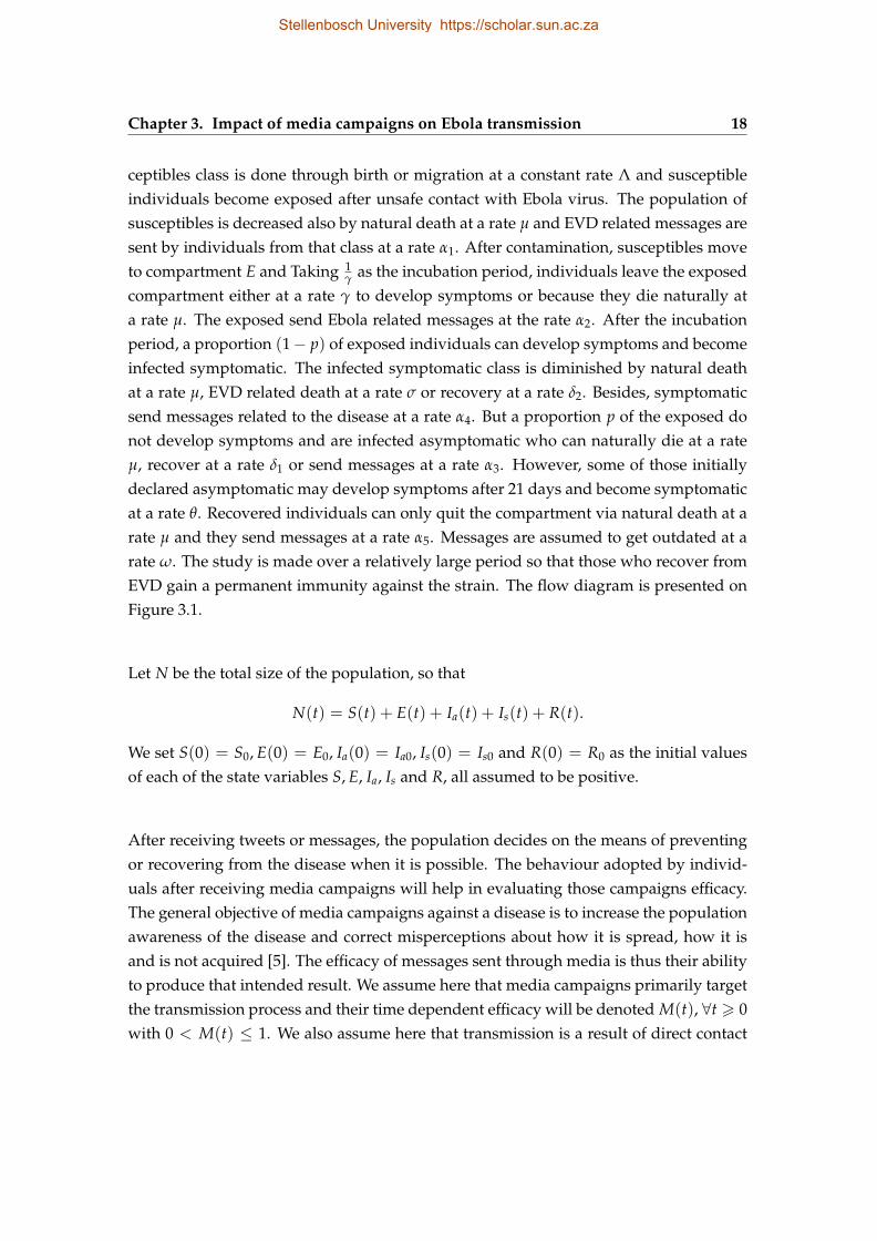
ceptibles class is done through birth or migration at a constant rate Λ and susceptibleindividuals become exposed after unsafe contact with Ebola virus. The population ofsusceptibles is decreased also by natural death at a rate µ and EVD related messages aresent by individuals from that class at a rate α1. After contamination, susceptibles moveto compartment E and Taking 1
γ as the incubation period, individuals leave the exposedcompartment either at a rate γ to develop symptoms or because they die naturally ata rate µ. The exposed send Ebola related messages at the rate α2. After the incubationperiod, a proportion (1− p) of exposed individuals can develop symptoms and becomeinfected symptomatic. The infected symptomatic class is diminished by natural deathat a rate µ, EVD related death at a rate σ or recovery at a rate δ2. Besides, symptomaticsend messages related to the disease at a rate α4. But a proportion p of the exposed donot develop symptoms and are infected asymptomatic who can naturally die at a rateµ, recover at a rate δ1 or send messages at a rate α3. However, some of those initiallydeclared asymptomatic may develop symptoms after 21 days and become symptomaticat a rate θ. Recovered individuals can only quit the compartment via natural death at arate µ and they send messages at a rate α5. Messages are assumed to get outdated at arate ω. The study is made over a relatively large period so that those who recover fromEVD gain a permanent immunity against the strain. The flow diagram is presented onFigure 3.1.
Let N be the total size of the population, so that
N(t) = S(t) + E(t) + Ia(t) + Is(t) + R(t).
We set S(0) = S0, E(0) = E0, Ia(0) = Ia0, Is(0) = Is0 and R(0) = R0 as the initial valuesof each of the state variables S, E, Ia, Is and R, all assumed to be positive.
After receiving tweets or messages, the population decides on the means of preventingor recovering from the disease when it is possible. The behaviour adopted by individ-uals after receiving media campaigns will help in evaluating those campaigns efficacy.The general objective of media campaigns against a disease is to increase the populationawareness of the disease and correct misperceptions about how it is spread, how it isand is not acquired [5]. The efficacy of messages sent through media is thus their abilityto produce that intended result. We assume here that media campaigns primarily targetthe transmission process and their time dependent efficacy will be denoted M(t), ∀t > 0with 0 < M(t) ≤ 1. We also assume here that transmission is a result of direct contact
Stellenbosch University https://scholar.sun.ac.za
19 3.2. Model formulation
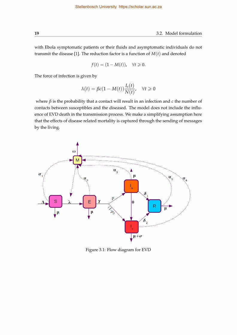
with Ebola symptomatic patients or their fluids and asymptomatic individuals do nottransmit the disease [1]. The reduction factor is a function of M(t) and denoted
f (t) = (1−M(t)), ∀t > 0.
The force of infection is given by
λ(t) = βc(1−M(t))Is(t)N(t)
, ∀t > 0
where β is the probability that a contact will result in an infection and c the number ofcontacts between susceptibles and the diseased. The model does not include the influ-ence of EVD death in the transmission process. We make a simplifying assumption herethat the effects of disease related mortality is captured through the sending of messagesby the living.
Figure 3.1: Flow diagram for EVD
Stellenbosch University https://scholar.sun.ac.za
Chapter 3. Impact of media campaigns on Ebola transmission 20
3.2.1 Model equations
Following the model assumptions and the description of the flow diagram, the systemof differential equations describing the dynamics of the model is as follows :
dSdt
= Λ− (λ + µ)S, (3.2.1)
dEdt
= cβ(1−M)Is
NS− (γ + µ)E, (3.2.2)
dIa
dt= pγE− (µ + θ + δ1)Ia, (3.2.3)
dIs
dt= (1− p)γE + θ Ia − (δ2 + σ + µ)Is, (3.2.4)
dRdt
= δ1 Ia + δ2 Is − µR, (3.2.5)
dMdt
= α1S + α2E + α3 Ia + α4 Is + α5R−ωM. (3.2.6)
3.3 Model properties and analysis
3.3.1 Existence and uniqueness of solutions
The right hand side of system (3.2.1)-(3.2.6) is made of Lipschitz continuous functionssince they describe the size of a population. According to Picard’s existence Theorem,with given initial conditions, the solutions of our system exist and they are unique.
Theorem 3.3.1. The system makes biological sense in the region
Ω = (S(t), E(t), Ia(t), Is(t), R(t), M(t)) ∈ R6 : N(t) 6Λµ
, 0 < M(t) 6 1
which is attracting and positively invariant with respect to the flow of system (3.2.1)-(3.2.6).
Proof. By adding equations (3.2.1) to equation (3.2.5) we have :
dNdt
= Λ− µN − σIs,
which implies
dNdt
6 Λ− µN. (3.3.1)
Using Corollary 3.3.4 we obtain
0 6 N(t) 6(
N(0)− Λµ
)exp(−µt) +
Λµ
, ∀ t > 0.
Stellenbosch University https://scholar.sun.ac.za
21 3.3. Model properties and analysis
We have limt→∞ N(t) <Λµ
when N(0) 6Λµ
. However, if N(0) >Λµ
, N(t)
will decrease toΛµ
. So N(t) is thus a bounded function of time. Together with M
which is already bounded, we can say that Ω is bounded and at limiting equilibrium
limt→∞ N(t) =Λµ
. Besides, any sum or difference of variables in Ω with positive initial
values will remain in Ω or in a neighbourhood of Ω. Thus Ω is positively invariant andattracting with respect to the flow of system (3.2.1)-(3.2.6).
3.3.2 Positivity of solutions
Theorem 3.3.2. The existing solutions of our system (3.2.1)-(3.2.6) are all positive.
Proof. From (3.2.1) we have
dSdt
= Λ− (λ(t) + µ)S, ∀t > 0, (3.3.2)
which implies
dSdt
> −(λ(t) + µ)S, ∀t > 0. (3.3.3)
SolvingdSdt
= −(λ(t) + µ)S yields
S(t) = S(0) exp[ ∫ t
0λ(u) du
]exp(−µ)t. (3.3.4)
Using (4.3.2) and (4.3.5) we obtain
S(t) > S(0) exp[ ∫ t
0λ(u) du
]exp(−µ)t (3.3.5)
which is positive given that S(0) is also positive.Similarly, from (3.2.2) we have
dEdt
> −(γ + µ)E ∀ t > 0,
so thatE(t) > E(0) exp[−(γ + µ)]t,
thus shows that E(t) is positive since E(0) is also positive.Similarly from (3.2.3) we can write
dIa
dt> −(µ + θ + δ1)Ia ∀t > 0,
Stellenbosch University https://scholar.sun.ac.za
Chapter 3. Impact of media campaigns on Ebola transmission 22
from which we obtainIa(t) > Ia(0) exp[−(µ + θ + δ1)]t.
Thus Ia is positive since Ia(0) is positive.The remaining equations yield
Is(t) > Is(0) exp−[(µ + σ + δ2)]t,
R(t) > R(0) exp(−µt)
andM(t) > M(0) exp(−ωt).
So Is(t), R(t) and M(t) are all positive for positive initial conditions. Thus all the statevariables are positive.
3.3.3 Steady states analysis
Our model has two steady states: the disease free equilibrium (DFE) which describes thetotal absence of EVD in the studied population and the endemic equilibrium (EE) whichexists at any positive prevalence of EVD in the population. This section is dedicated tothe study of local and global stability of these steady states.
3.3.4 The disease free equilibrium and RM
At the disease free equilibrium (S, E, Ia, Is, R, M) = (S∗, 0, 0, 0, 0, M∗). The resolution ofthe following system
−µS∗ + Λ = 0,
α1S−ωM∗ = 0,
yields
S∗ =Λµ
and M∗ =Λα1
ωµ.
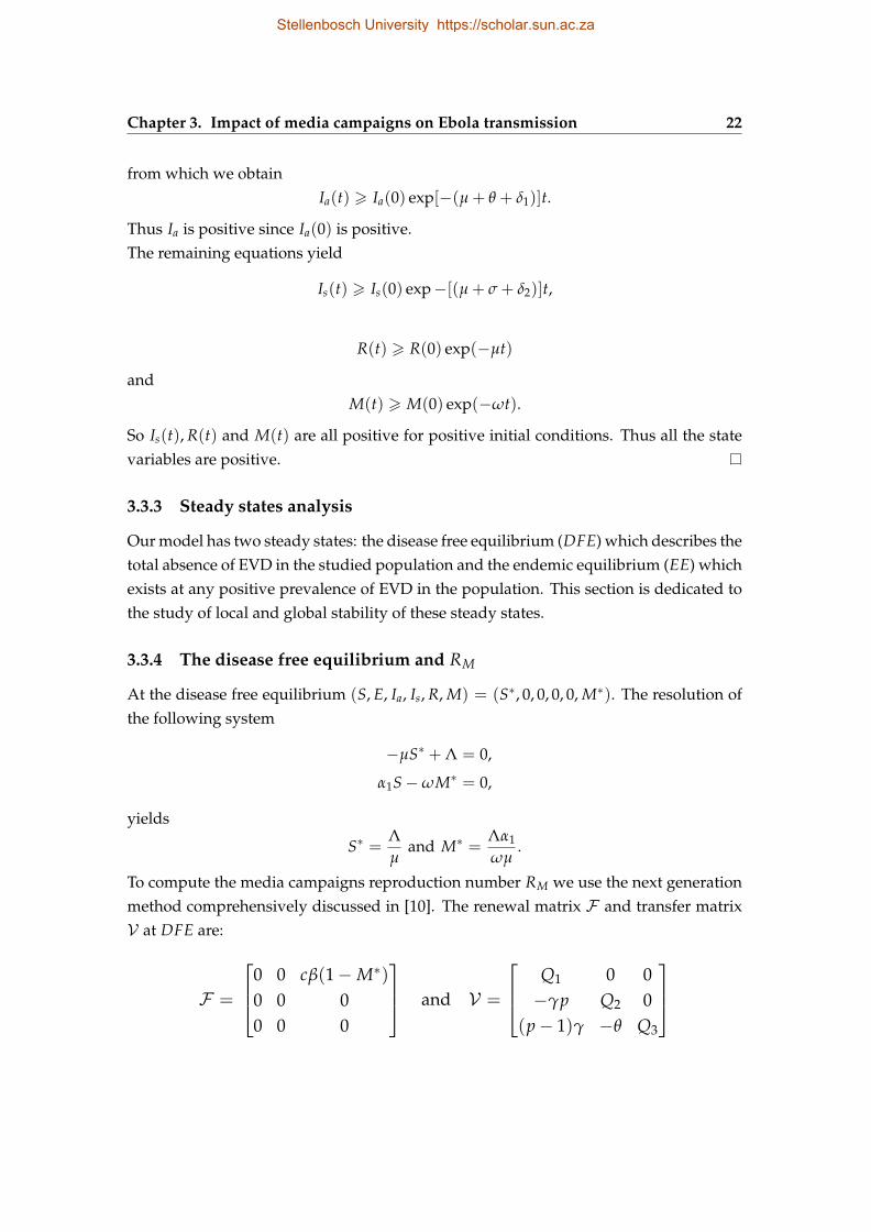
To compute the media campaigns reproduction number RM we use the next generationmethod comprehensively discussed in [10]. The renewal matrix F and transfer matrixV at DFE are:
F =
0 0 cβ(1−M∗)0 0 00 0 0
and V =
Q1 0 0−γp Q2 0
(p− 1)γ −θ Q3
Stellenbosch University https://scholar.sun.ac.za
23 3.3. Model properties and analysis
where
Q1 = γ + µ, Q2 = µ + θ + δ1 and Q3 = δ2 + σ + µ.
The media campaigns reproduction number RM is the spectral radius of the ma-trix FV−1 and is given by
RM =cβγ(1−M∗)
Q1Q2Q3
[pθ + (1− p)Q2
].
We can write RM = R1 + R2 for elucidation purpose with
R1 =( pcβ(1−M∗)
Q3
)( γ
Q1
)( θ
Q2
), R2 =
( cβ(1− p)(1−M∗)Q3
)( γ
Q1
).
Note here that1
Q3is the duration of infectivity for the symptomatic,
θ
Q2the
probability that an individual in Ia moves to Is andγ
Q1the probability that an
individual in E moves either to Ia or Is. Thus, the media campaigns reproductionnumber is a sum of secondary infections due to the infectious individuals (R1) inIs and the asymptomatic individuals who become infectious (R2). We can noticethe reduction factor 0 6 (1−M∗) < 1 which represents the attenuating effect ofmedia campaigns on the future number of EVD cases.
3.3.4.1 Local and global stability
The description of the DFE stability is given below.
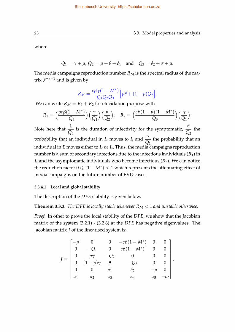
Theorem 3.3.3. The DFE is locally stable whenever RM < 1 and unstable otherwise.
Proof. In other to prove the local stability of the DFE, we show that the Jacobianmatrix of the system (3.2.1) - (3.2.6) at the DFE has negative eigenvalues. TheJacobian matrix J of the linearised system is:
J =
−µ 0 0 −cβ(1−M∗) 0 00 −Q1 0 cβ(1−M∗) 0 00 pγ −Q2 0 0 00 (1− p)γ θ −Q3 0 00 0 δ1 δ2 −µ 0α1 α2 α3 α4 α5 −ω
.
Stellenbosch University https://scholar.sun.ac.za
Chapter 3. Impact of media campaigns on Ebola transmission 24
The characteristic equation of J is given by :
(ζ + µ)2(ζ + ω)(ζ3 + a1ζ2 + a2ζ + a3) = 0 (3.3.6)
with
a1 =Q1 + Q2 + Q3,
a2 =cβγ(1−M∗)(p− 1) + Q1Q2 + Q3Q2 + Q1Q3,
=Q1Q3
(1− R2
)+ Q1Q2 + Q3Q2,
a3 =Q1Q2Q3[1−cβγ(1−M∗)
Q1Q2Q3
(pθ + (1− p)Q2
)].
=Q1Q2Q3(1− RM).
Since −µ (twice) and −ω are negative roots of the characteristic polynomial(3.3.6), we use Routh-Hurwitz criterion to show that the remaining polynomial
ζ3 + a1ζ2 + a2ζ + a3 = 0
has negative real roots.The first condition for these criteria to be used is that a3 must be positive andclearly when RM < 1, a1, a2 and a3 are all positive. In addition, a1a2 − a3 mustbe positive to have negative real roots for the polynomial. We thus have
a1a2 − a3 = Q1Q3(Q2 + Q3)(1− R2) + Q1Q2 + Q3Q2Q1RM,
so a1a2 − a3 > 0 since R2 < RM < 1. The necessary and sufficient conditionfor the Jacobian matrix J to have negative roots is that the reproduction numberis less than one. From the Routh-Hurwitz stability criterion, we can concludethat the DFE is locally asymptotically stable when RM < 1 and unstable forRM > 1.
Corollary 3.3.4. Let x0, y0 be real numbers, I = [x0,+∞) and a, b ∈ C(I). Supposethat y ∈ C1(I) satisfies the following inequality
y′(x) 6 a(x)y(x) + b(x), x > x0, y(x0) = y0. (3.3.7)
Stellenbosch University https://scholar.sun.ac.za
25 3.3. Model properties and analysis
Then
y(x) 6 y0 exp
( x∫x0
a(t) dt
)+∫ x
x0
b(s) exp
( ∫ x
sa(t) dt
)ds, x > x0. (3.3.8)
If the converse inequality holds in (3.3.7), then the converse inequality holds in (3.3.8)too.
3.3.5 Existence and stability of the endemic equilibrium
In this section we show the existence of the endemic equilibrium (EE). We de-note the endemic equilibrium by (S∗∗, E∗∗, I∗∗a , I∗∗s , R∗∗, M∗∗). At equilibrium,
Λ− (λ + µ)S = 0, (3.3.9)
cβ(1−M)Is
NS− (γ + µ)E = 0, (3.3.10)
pγE− (µ + θ + δ1)Ia = 0, (3.3.11)
(1− p)γE + θ Ia − (δ2 + σ + µ)Is = 0, (3.3.12)
δ1 Ia + δ2 Is − µR = 0, (3.3.13)
α1S + α2E + α3 Ia + α4 Is + α5R−ωM = 0. (3.3.14)
Thus, from equation (3.3.9) we have
S∗∗ =1
λ∗∗ + µQ1Q2Q3.
From equation (3.3.10) we have
E∗∗ =λ∗∗
(λ∗∗ + µ)Q2Q3,
from equation (3.3.11) we have
I∗∗a =pγλ∗∗
(λ∗∗ + µ)Q3,
from equation (3.3.12) we have
I∗∗s =γλ∗∗
[pθ + Q2(1− p)
](λ∗∗ + µ)
,
Stellenbosch University https://scholar.sun.ac.za
Chapter 3. Impact of media campaigns on Ebola transmission 26
from equation (3.3.13) we have
R∗∗ =γλ∗∗
[p(Q3δ1 + θδ2) + Q2δ2(1− p)
]µ(λ∗∗ + µ)
and from equation (3.3.14) we have
M∗∗ =1
µω(λ∗∗ + µ)(φ1 + φ2λ∗∗)
whereλ∗∗ = βc(1−M∗∗)
I∗∗sN∗∗
,
φ1 = µQ1Q2Q3α1
and
φ2 = γ(µα4 + α5δ2)(pθ + (1− p)Q2) + Q3
(µ(Q2α2 + pγα3) + pγα5δ1
).
Set P(λ∗∗) = λ∗∗ − βc(1 − M∗∗) I∗∗sN∗∗ . By replacing M∗∗, I∗∗s and N∗∗ by their
values expressed as functions of λ∗∗ and by setting
P(λ∗∗) = 0
we obtain the following equation:
Λλ∗∗[(ν2(λ∗∗)2 + ν1λ∗∗ + ν0)] = 0 (3.3.15)
where
ν0 = ωQ1Q2Q3µ(1− RM),
ν1 = µωQ21Q2
2Q23 + ωQ1Q2Q3Σ,
ν2 = ωQ1Q2Q3
[γ(µ + δ2)(pθ + (1− p)Q2) + µ(Q3(Q2 + pγ(µ + δ1)))
]> 0,
(3.3.16)
with Σ =[− γ(cβ − µ)(pθ + Q2(1− p)) + µφ2(pγ + Q2)Q3
]µ + γµ
[pQ3δ1 +
(pθ + Q2(1− p)δ2)]+ cβγΛ
[pθ + (1− p)Q2
].
Stellenbosch University https://scholar.sun.ac.za
27 3.3. Model properties and analysis
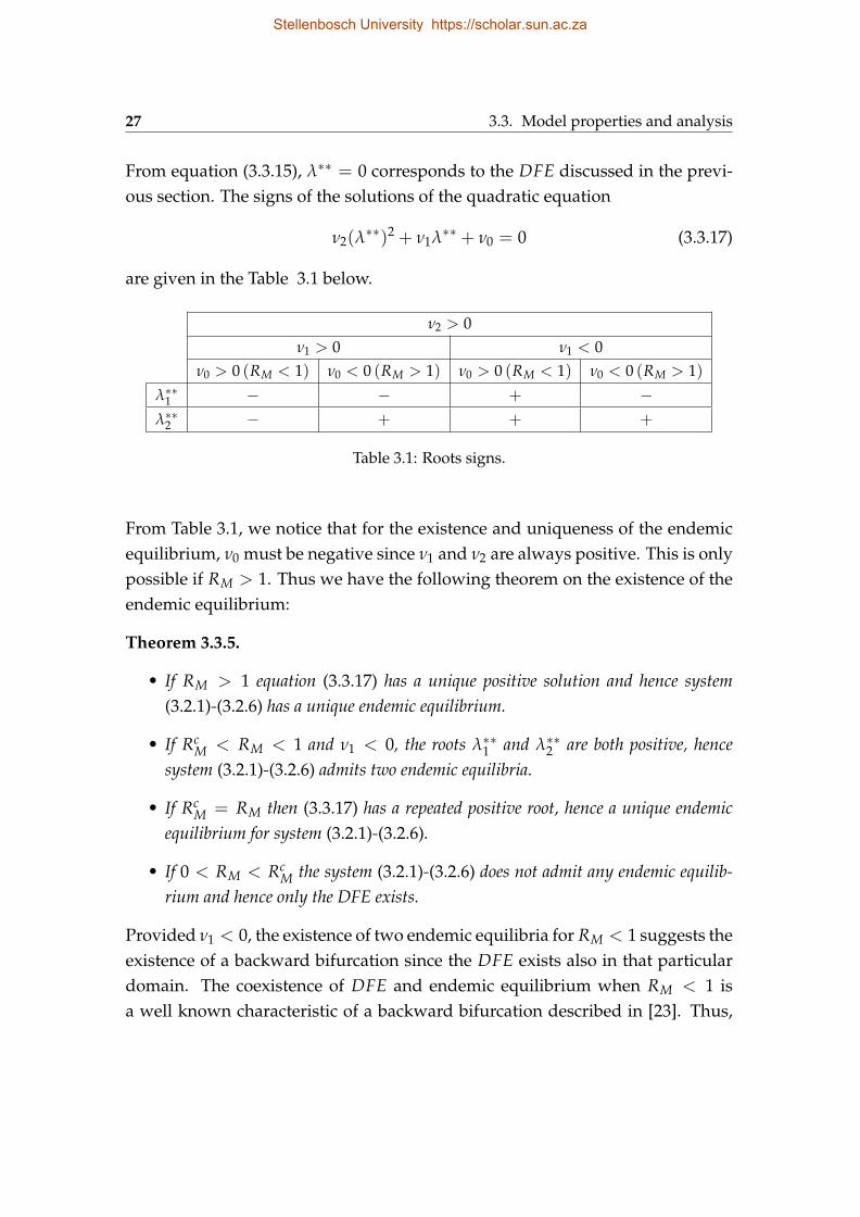
From equation (3.3.15), λ∗∗ = 0 corresponds to the DFE discussed in the previ-ous section. The signs of the solutions of the quadratic equation
ν2(λ∗∗)2 + ν1λ∗∗ + ν0 = 0 (3.3.17)
are given in the Table 3.1 below.
ν2 > 0ν1 > 0 ν1 < 0
ν0 > 0 (RM < 1) ν0 < 0 (RM > 1) ν0 > 0 (RM < 1) ν0 < 0 (RM > 1)
λ∗∗1 − − + −λ∗∗2 − + + +
Table 3.1: Roots signs.
From Table 3.1, we notice that for the existence and uniqueness of the endemicequilibrium, ν0 must be negative since ν1 and ν2 are always positive. This is onlypossible if RM > 1. Thus we have the following theorem on the existence of theendemic equilibrium:
Theorem 3.3.5.
• If RM > 1 equation (3.3.17) has a unique positive solution and hence system(3.2.1)-(3.2.6) has a unique endemic equilibrium.
• If RcM < RM < 1 and ν1 < 0, the roots λ∗∗1 and λ∗∗2 are both positive, hence
system (3.2.1)-(3.2.6) admits two endemic equilibria.
• If RcM = RM then (3.3.17) has a repeated positive root, hence a unique endemic
equilibrium for system (3.2.1)-(3.2.6).
• If 0 < RM < RcM the system (3.2.1)-(3.2.6) does not admit any endemic equilib-
rium and hence only the DFE exists.
Provided ν1 < 0, the existence of two endemic equilibria for RM < 1 suggests theexistence of a backward bifurcation since the DFE exists also in that particulardomain. The coexistence of DFE and endemic equilibrium when RM < 1 isa well known characteristic of a backward bifurcation described in [23]. Thus,
Stellenbosch University https://scholar.sun.ac.za
Chapter 3. Impact of media campaigns on Ebola transmission 28
there exists a critical value of RM called here RcM for which there is a change in
the qualitative behaviour of our model.At the bifurcation point, there is an intersection between the line RM = Rc
M andthe graph of P(λ∗∗). Thus the discriminant ∆ is equal to zero at RM = Rc
M, whichmathematically is
ν21 − 4ωQ1Q2Q3µ(1− Rc
M)ν2 = 0
from which
RcM = 1−
ν21
4ψν2.
Theorem 3.3.6. Given that RcM = 1−
ν21
4ψν2, with ψ = ωQ1Q2Q3µ, ν1 and ν2 are
defined in (3.3.16) , the DFE is globally asymptotically stable whenever RM < RcM.
Proof. To show the global stability of the DFE we use the Invariance Principle ofLassale [43]. Let us set V(t) = E(t) + Ia(t) + Is(t) as our Lyapunov function.
V(t) > 0 since E(t) > 0, Ia(t) > 0, Is(t) > 0, ∀t > 0.
V(t) = 0 if E(t) = Ia(t) = Is(t) = 0 (at DFE).
Thus V is a positive definite function at the DFE.From equation (3.2.6) we have
dMdt
> α1S−ωM.
By applying Corollary 3.3.4 we have
M(t) > M(0) exp
( t∫0
(−ω) du
)+∫ t
0α1S exp
( ∫ t
z(−ω) dv
)dz, ∀t > 0
which yields
M(t) > exp(−ωt)(
M(0)− α1Sω
)+
α1Sω
. (3.3.18)
Before the disease is spread, we assume that M is at the steady state level. So
M(0) =α1Sω
which is equivalent to M(0) = M∗ and (3.3.18) will give
M(t) >α1Sω
.
Stellenbosch University https://scholar.sun.ac.za
29 3.3. Model properties and analysis
Together with the assumption 0 < M 6 1 we thus have
M∗ 6 M(t) 6 1.
The derivative of V is given by
V = E + Ia + Is,
=(
cβ(1−M)SN−Q3
)Is + (γ−Q1)E + (θ −Q2)Ia.
Since S 6 N,SN
6 1 and in addition M(t) > M∗. We thus have
V 6 [cβ(1−M∗)−Q3]Is + (γ−Q1)E + (θ −Q2)Ia. (3.3.19)
At equilibrium,
cβ(1−M)Is
NS− (γ + µ)E = 0, (3.3.20)
pγE− (µ + θ + δ1)Ia = 0, (3.3.21)
(1− p)γE + θ Ia − (δ2 + σ + µ)Is = 0. (3.3.22)
From equation (3.3.21) we have
E =Q2
pγIa. (3.3.23)
From equation (3.3.22) we have
Is =(pθ + (1− p)Q2)
pQ3Ia. (3.3.24)
By plugging (3.3.23) and (3.3.24) in (3.3.19) we obtain after simplifications
V 6−Q1Q2
p
[1− cβγ(1−M∗)
(pθ + (1− p)Q2)
Q1Q2Q3
]Ia,
6−Q1Q2
p
[1− RM
]Ia,
6−Q1Q2Q3[
pθ + (1− p)Q2
] (1− RM)Is.
Stellenbosch University https://scholar.sun.ac.za
Chapter 3. Impact of media campaigns on Ebola transmission 30
Thus V 6 0 when RM 6 1 and particularly, V = 0 only if E = Ia = Is = 0.Because the largest invariant set for which V = 0 in Ω is the DFE and V 6 0if RM 6 1, by using the Invariance Principle of Lassale [43] we can concludethat the DFE is globally asymptotically stable for RM 6 1. Together with theexistence of a backward bifurcation, one can say that for RM < Rc
M the DFE isglobally stable.
Remark 3.3.7.0 < RM < Rc
M the DFE is globally stable,
RcM < RM < 1 the DFE is locally stable and two endemic equilibria exist
with one which is stable and the other one unstable.
3.4 Local stability of endemic equilibrium
The DFE and EE both describe different qualitative behaviours of our epidemic.Let us set φ = cβ(1−M∗) as our bifurcation parameter, so that for
RM = 1, φ = φ∗ =Q1Q2Q3
γ(pθ + (1− p)Q2).
In order to describe the stability of the endemic equilibrium, we will use thetheorem, remark and corollary in [7] which are based on the Centre ManifoldTheory.
Theorem 3.4.1. Consider a general system of ordinary differential equations with aparameter φ:
dxdt
= f (x, φ), f : Rn ×R −→ Rn and f ∈ C2(Rn ×R). (3.4.1)
Without loss of generality, it is assumed that 0 is an equilibrium for system (3.4.1) forall values of the parameter φ, that is f (0, φ) ≡ 0 for all φ.
Assume
A1 : A = Dx f (0, 0) =
(∂ fi
∂ xj(0, 0)
)is the linearisation matrix of System (3.4.1)
around the equilibrium 0 with φ evaluated at 0. Zero is a simple eigenvalue of A and allother eigenvalues of A have negative real parts;
Stellenbosch University https://scholar.sun.ac.za
31 3.4. Local stability of endemic equilibrium
A2: Matrix A has a non negative right eigenvector w and a left eigenvector v corre-sponding to the zero eigenvalue. Let fk be the kth component of f and
a =n
∑k,i,j=1
vkwiwj∂2 fk
∂xi∂xj(0, 0), b =
n
∑k,i=1
vkwi∂2 fk∂xi∂φ
(0, 0).
The local dynamics of (3.4.1) around 0 are totally determined by a and b.
1. a > 0, b > 0. When φ < 0 with | φ | 1, 0 is locally asymptotically stable, andthere exists a positive unstable equilibrium; when 0 < φ 1, 0 is unstable andthere exists a negative and locally asymptotically stable equilibrium;
2. a < 0, b < 0. When φ < 0 with | φ | 1, 0 is unstable; when 0 < φ 1, 0 islocally asymptotically stable, and there exists a positive unstable equilibrium;
3. a > 0, b < 0. When φ < 0 with | φ | 1 , 0 is unstable, and there exists a locallyasymptotically stable negative equilibrium; when 0 < φ 1, 0 is stable, and apositive unstable equilibrium appears;
4. a < 0, b > 0. When φ changes from negative to positive, 0 changes its stabilityfrom stable to unstable. Correspondingly a negative unstable equilibrium becomespositive and locally asymptotically stable.
Corollary 3.4.2. When a > 0 and b > 0, the bifurcation at φ = 0 is subcritical orbackward.
For the model (3.2.1)-(3.2.6), the DFE (E0) is not equal to zero. According toRemark 1 in [7], we notice that if the equilibrium of interest in Theorem (3.4.1)is a non-negative equilibrium x0, then the requirement that w is non negative inTheorem (3.4.1) is not necessary. When some components in w are negative, onecan still apply Theorem (3.4.1) on condition that:w(j) > 0 if x0(j) = 0,
if x0(j) > 0, w(j) does not need to be positive,
where w(j) and x0(j) denote the jth component of w and x0 respectively.
Stellenbosch University https://scholar.sun.ac.za
Chapter 3. Impact of media campaigns on Ebola transmission 32
First, let us rewrite system (3.2.1)-(3.2.6) introducing
S = x1, E = x2, Ia = x3, Is = x4, R = x5, M = x6
andS = f1, E = f2, Ia = f3, Is = f4, R = f5, M = f6.
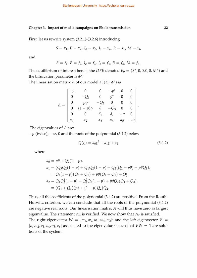
The equilibrium of interest here is the DFE denoted E0 = (S∗, 0, 0, 0, 0, M∗) andthe bifurcation parameter is φ∗.The linearisation matrix A of our model at (E0, φ∗) is
A =
−µ 0 0 −φ∗ 0 00 −Q1 0 φ∗ 0 00 pγ −Q2 0 0 00 (1− p)γ θ −Q3 0 00 0 δ1 δ2 −µ 0α1 α2 α3 α4 α5 −ω
.
The eigenvalues of A are:−µ (twice), −ω, 0 and the roots of the polynomial (3.4.2) below
Q(ς) = a0ς2 + a1ς + a2 (3.4.2)
where
a0 = pθ + Q2(1− p),
a1 = (Q3Q2(1− p) + Q1Q2(1− p) + Q2(Q2 + pθ) + pθQ1),
= Q2(1− p)(Q3 + Q1) + pθ(Q2 + Q1) + Q22,
a2 = Q1Q22(1− p) + Q2
2Q3(1− p) + pθQ2(Q1 + Q3),
= (Q1 + Q3)(pθ + (1− p)Q2)Q2.
Thus, all the coefficients of the polynomial (3.4.2) are positive. From the Routh-Hurwitz criterion, we can conclude that all the roots of the polynomial (3.4.2)are negative real roots. Our linearisation matrix A will thus have zero as largesteigenvalue. The statement A1 is verified. We now show that A2 is satisfied.The right eigenvector W = [w1, w2, w3, w4, w5]
′ and the left eigenvector V =
[v1, v2, v3, v4, v5, v6] associated to the eigenvalue 0 such that VW = 1 are solu-tions of the system:
Stellenbosch University https://scholar.sun.ac.za
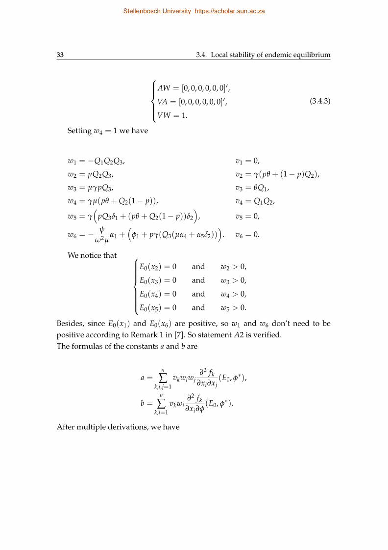
33 3.4. Local stability of endemic equilibrium
AW = [0, 0, 0, 0, 0, 0]′,
VA = [0, 0, 0, 0, 0, 0]′,
VW = 1.
(3.4.3)
Setting w4 = 1 we have
w1 = −Q1Q2Q3, v1 = 0,
w2 = µQ2Q3, v2 = γ(pθ + (1− p)Q2),
w3 = µγpQ3, v3 = θQ1,
w4 = γµ(pθ + Q2(1− p)), v4 = Q1Q2,
w5 = γ(
pQ3δ1 + (pθ + Q2(1− p))δ2
), v5 = 0,
w6 = − ψ
ω2µα1 +
(φ1 + pγ(Q3(µα4 + α5δ2))
). v6 = 0.
We notice that
E0(x2) = 0 and w2 > 0,
E0(x3) = 0 and w3 > 0,
E0(x4) = 0 and w4 > 0,
E0(x5) = 0 and w5 > 0.
Besides, since E0(x1) and E0(x6) are positive, so w1 and w6 don’t need to bepositive according to Remark 1 in [7]. So statement A2 is verified.The formulas of the constants a and b are
a =n
∑k,i,j=1
vkwiwj∂2 fk
∂xi∂xj(E0, φ∗),
b =n
∑k,i=1
vkwi∂2 fk∂xi∂φ
(E0, φ∗).
After multiple derivations, we have
Stellenbosch University https://scholar.sun.ac.za
Chapter 3. Impact of media campaigns on Ebola transmission 34
a = −2Q1Q2Q3γ((µ + δ2)(pθ + (1− p)Q2) + pQ3(µ + δ1)) + Q2Q3µ
γ(Q2(Q3 + Q1)(pθ + (1− p)Q2) + pθQ3)µS∗< 0
and
b =γ(pθ + (1− p)Q2)
2
Q2(pθ + (1− p)Q2)(Q3 + Q1) + pθQ3> 0.
Since a < 0 and b > 0, by using the fourth item of Theorem 3.4.1 we can con-clude that when φ∗ changes from negative to positive, E0 changes its stabilityfrom stable to unstable. Correspondingly a negative unstable equilibrium be-comes positive and locally asymptotically stable and a forward bifurcation ap-pears [23].
Theorem 3.4.3. A unique endemic equilibrium exists when RM > 1 and is locallyasymptotically stable.
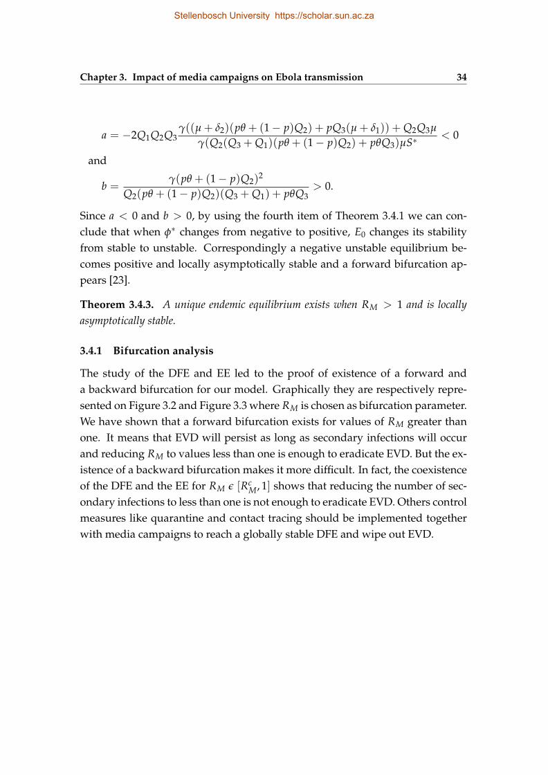
3.4.1 Bifurcation analysis
The study of the DFE and EE led to the proof of existence of a forward anda backward bifurcation for our model. Graphically they are respectively repre-sented on Figure 3.2 and Figure 3.3 where RM is chosen as bifurcation parameter.We have shown that a forward bifurcation exists for values of RM greater thanone. It means that EVD will persist as long as secondary infections will occurand reducing RM to values less than one is enough to eradicate EVD. But the ex-istence of a backward bifurcation makes it more difficult. In fact, the coexistenceof the DFE and the EE for RM ε [Rc
M, 1] shows that reducing the number of sec-ondary infections to less than one is not enough to eradicate EVD. Others controlmeasures like quarantine and contact tracing should be implemented togetherwith media campaigns to reach a globally stable DFE and wipe out EVD.
Stellenbosch University https://scholar.sun.ac.za
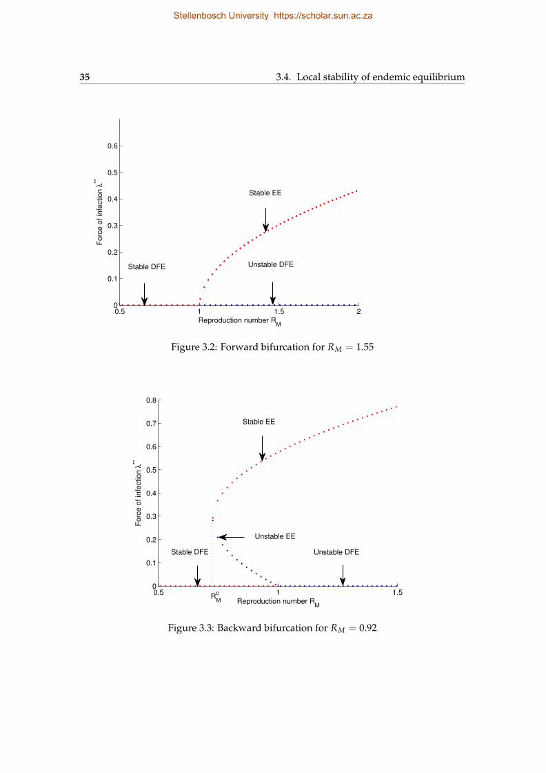
35 3.4. Local stability of endemic equilibrium
0.5 1 1.5 20
0.1
0.2
0.3
0.4
0.5
0.6
Reproduction number RM
Forc
e o
f in
fection λ
**
Stable DFE Unstable DFE
Stable EE
Figure 3.2: Forward bifurcation for RM = 1.55
0.5 1 1.50
0.1
0.2
0.3
0.4
0.5
0.6
0.7
0.8
Reproduction number RM
Forc
e o
f in
fection λ
**
RM
c
Stable DFE
Stable EE
Unstable DFE
Unstable EE
Figure 3.3: Backward bifurcation for RM = 0.92
Stellenbosch University https://scholar.sun.ac.za
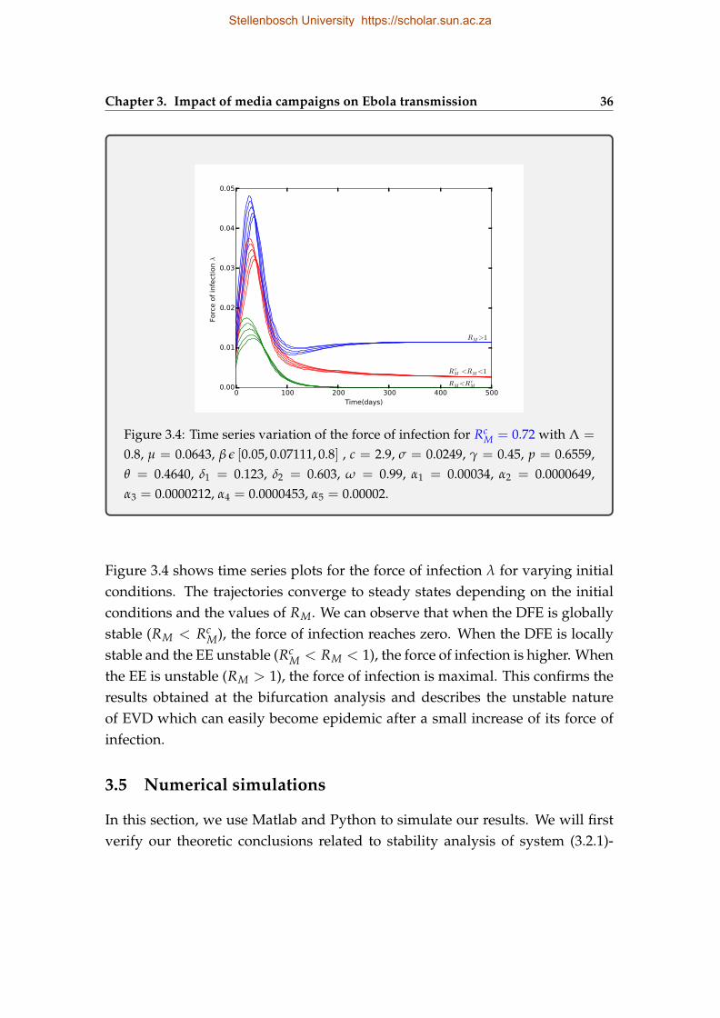
Chapter 3. Impact of media campaigns on Ebola transmission 36
0 100 200 300 400 500Time(days)
0.00
0.01
0.02
0.03
0.04
0.05
Force of in
fection λ
RM<RcM
R cM <RM<1
RM>1
Figure 3.4: Time series variation of the force of infection for RcM = 0.72 with Λ =
0.8, µ = 0.0643, β ε [0.05, 0.07111, 0.8] , c = 2.9, σ = 0.0249, γ = 0.45, p = 0.6559,θ = 0.4640, δ1 = 0.123, δ2 = 0.603, ω = 0.99, α1 = 0.00034, α2 = 0.0000649,α3 = 0.0000212, α4 = 0.0000453, α5 = 0.00002.
Figure 3.4 shows time series plots for the force of infection λ for varying initialconditions. The trajectories converge to steady states depending on the initialconditions and the values of RM. We can observe that when the DFE is globallystable (RM < Rc
M), the force of infection reaches zero. When the DFE is locallystable and the EE unstable (Rc
M < RM < 1), the force of infection is higher. Whenthe EE is unstable (RM > 1), the force of infection is maximal. This confirms theresults obtained at the bifurcation analysis and describes the unstable natureof EVD which can easily become epidemic after a small increase of its force ofinfection.
3.5 Numerical simulations
In this section, we use Matlab and Python to simulate our results. We will firstverify our theoretic conclusions related to stability analysis of system (3.2.1)-
Stellenbosch University https://scholar.sun.ac.za
37 3.5. Numerical simulations
(3.2.6), then we will vary our parameters values to better understand how me-dia campaigns influence the prevalence and transmission of EVD. Then will befollowed by data fitting in the model validation process.
Hypothetically, we choose a population of size 960. The initial conditions chosenwil be
S0 = 900, E0 = 50, Ia0 = 0, Is0 = 10, R0 = 0, M0 = 0.4.
It is important to note that the figures chosen are for illustrative purposes only,as we endeavour to verify the analytic results.
3.5.1 Parameters estimation
The parameters used in the simulations are either obtained from literature orestimated. Since the mean infectious period is set to be from 4 to 10 days, thehighest recovery rate δ2 is set to 1/4. The recovery rate of asymptomatic individ-uals is assumed to be greater than the one of the symptomatic individuals sincethe former have a stronger resistance to the EVD. Without any reliable sourcefor EVD related media data, we assume that everyone can send EVD relatedmessages through media. At the beginning of the epidemic, there is neither arecovered or asymptomatic infected individual since only symptomatic personstransmit the disease. We also assume that messages are transmitted through me-dia at time t = 0, at least for a preventive purposes.
Table 3.2 below gives more details about the parameters values.
Stellenbosch University https://scholar.sun.ac.za
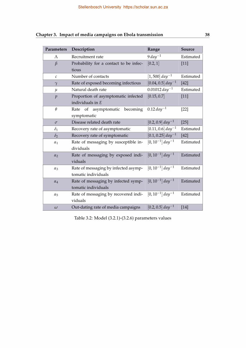
Chapter 3. Impact of media campaigns on Ebola transmission 38
Parameters Description Range Source
Λ Recruitment rate 9 day−1 Estimated
β Probability for a contact to be infec-tious
[0.2, 1] [11]
c Number of contacts [1, 500] day−1 Estimated
γ Rate of exposed becoming infectious [0.04, 0.5] day−1 [42]
µ Natural death rate 0.01012 day−1 Estimated
p Proportion of asymptomatic infectedindividuals in E
[0.15, 0.7] [11]
θ Rate of asymptomatic becomingsymptomatic
0.12 day−1 [22]
σ Disease related death rate [0.2, 0.9] day−1 [25]
δ1 Recovery rate of asymptomatic [0.11, 0.6] day−1 Estimated
δ2 Recovery rate of symptomatic [0.1, 0.25] day−1 [42]
α1 Rate of messaging by susceptible in-dividuals
[0, 10−1] day−1 Estimated
α2 Rate of messaging by exposed indi-viduals
[0, 10−1] day−1 Estimated
α3 Rate of messaging by infected asymp-tomatic individuals
[0, 10−1] day−1 Estimated
α4 Rate of messaging by infected symp-tomatic individuals
[0, 10−1] day−1 Estimated
α5 Rate of messaging by recovered indi-viduals
[0, 10−1] day−1 Estimated
ω Out-dating rate of media campaigns [0.2, 0.5] day−1 [14]
Table 3.2: Model (3.2.1)-(3.2.6) parameters values
Stellenbosch University https://scholar.sun.ac.za
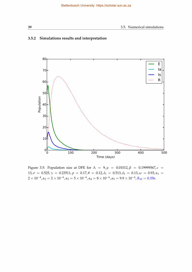
39 3.5. Numerical simulations
3.5.2 Simulations results and interpretation
0 100 200 300 400 500Time (days)
0
10
20
30
40
50
60
70
80
Popu
latio
n
EIaIsR
Figure 3.5: Population size at DFE for Λ = 9, µ = 0.01012, β = 0.19999567, c =
13, σ = 0.525, γ = 0.23511, p = 0.17, θ = 0.12, δ1 = 0.513, δ2 = 0.13, ω = 0.93, α1 =
2× 10⁻⁴, α2 = 2× 10⁻⁶, α3 = 5× 10⁻⁶, α4 = 8× 10⁻⁶, α5 = 9.9× 10⁻⁶, RM = 0.356.
Stellenbosch University https://scholar.sun.ac.za
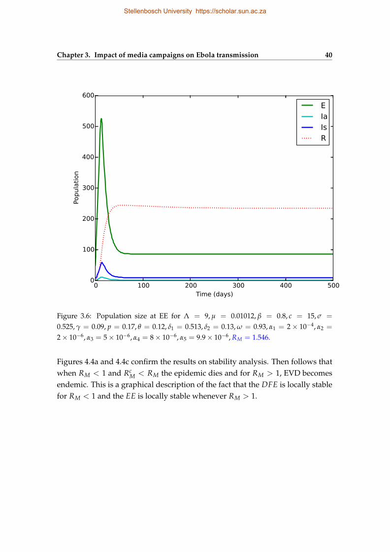
Chapter 3. Impact of media campaigns on Ebola transmission 40
0 100 200 300 400 500Time (days)
0
100
200
300
400
500
600
Popu
latio
n
EIaIsR
Figure 3.6: Population size at EE for Λ = 9, µ = 0.01012, β = 0.8, c = 15, σ =
0.525, γ = 0.09, p = 0.17, θ = 0.12, δ1 = 0.513, δ2 = 0.13, ω = 0.93, α1 = 2× 10⁻⁴, α2 =
2× 10⁻⁶, α3 = 5× 10⁻⁶, α4 = 8× 10⁻⁶, α5 = 9.9× 10⁻⁶, RM = 1.546.
Figures 4.4a and 4.4c confirm the results on stability analysis. Then follows thatwhen RM < 1 and Rc
M < RM the epidemic dies and for RM > 1, EVD becomesendemic. This is a graphical description of the fact that the DFE is locally stablefor RM < 1 and the EE is locally stable whenever RM > 1.
Stellenbosch University https://scholar.sun.ac.za
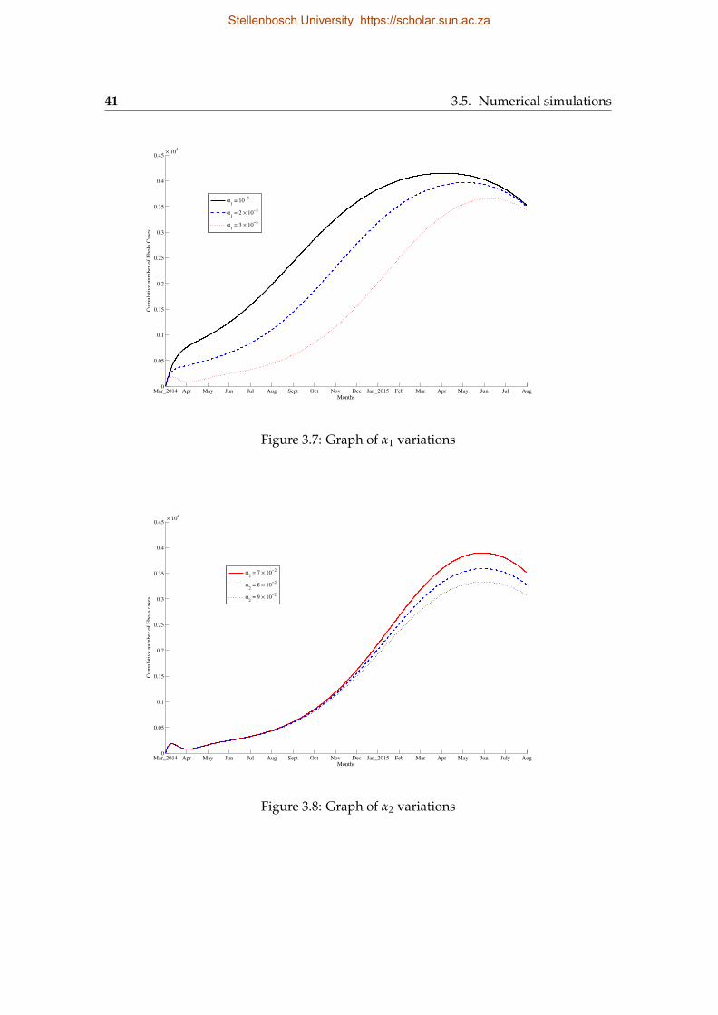
41 3.5. Numerical simulations
Mar_2014 Apr May Jun Jul Aug Sept Oct Nov Dec Jan_2015 Feb Mar Apr May Jun Jul Aug0
0.05
0.1
0.15
0.2
0.25
0.3
0.35
0.4
0.45
Months
Cu
mu
lati
ve
nu
mb
er o
f E
bo
la C
ases
α1 = 10
−5
α1 = 2 × 10
−5
α1 = 3 × 10
−5
× 104
Figure 3.7: Graph of α1 variations
Mar_2014 Apr May Jun Jul Aug Sept Oct Nov Dec Jan_2015 Feb Mar Apr May Jun July Aug0
0.05
0.1
0.15
0.2
0.25
0.3
0.35
0.4
0.45
Months
Cum
ula
tiv
e num
ber
of
Ebo
la c
ases
α2 = 7 × 10
−2
α2 = 8 × 10
−2
α2 = 9 × 10
−2
× 104
Figure 3.8: Graph of α2 variations
Stellenbosch University https://scholar.sun.ac.za
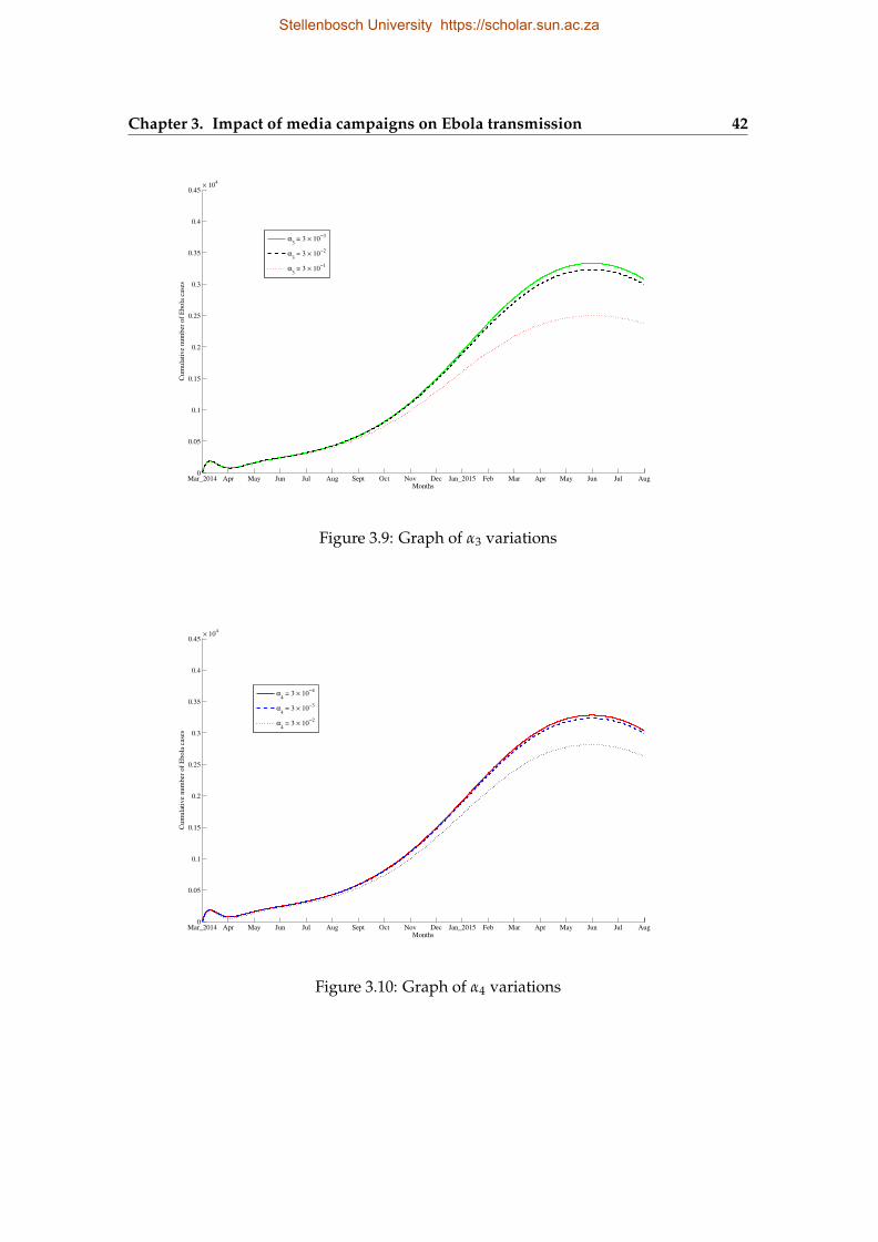
Chapter 3. Impact of media campaigns on Ebola transmission 42
Mar_2014 Apr May Jun Jul Aug Sept Oct Nov Dec Jan_2015 Feb Mar Apr May Jun Jul Aug0
0.05
0.1
0.15
0.2
0.25
0.3
0.35
0.4
0.45
Months
Cu
mu
lati
ve
nu
mb
er o
f E
bola
cas
es
α3 = 3 × 10
−3
α3 = 3 × 10
−2
α3 = 3 × 10
−1
× 104
Figure 3.9: Graph of α3 variations
Mar_2014 Apr May Jun Jul Aug Sept Oct Nov Dec Jan_2015 Feb Mar Apr May Jun Jul Aug0
0.05
0.1
0.15
0.2
0.25
0.3
0.35
0.4
0.45
Months
Cum
ula
tiv
e num
ber
of
Ebo
la c
ases
α4 = 3 × 10
−4
α4 = 3 × 10
−3
α4 = 3 × 10
−2
× 104
Figure 3.10: Graph of α4 variations
Stellenbosch University https://scholar.sun.ac.za
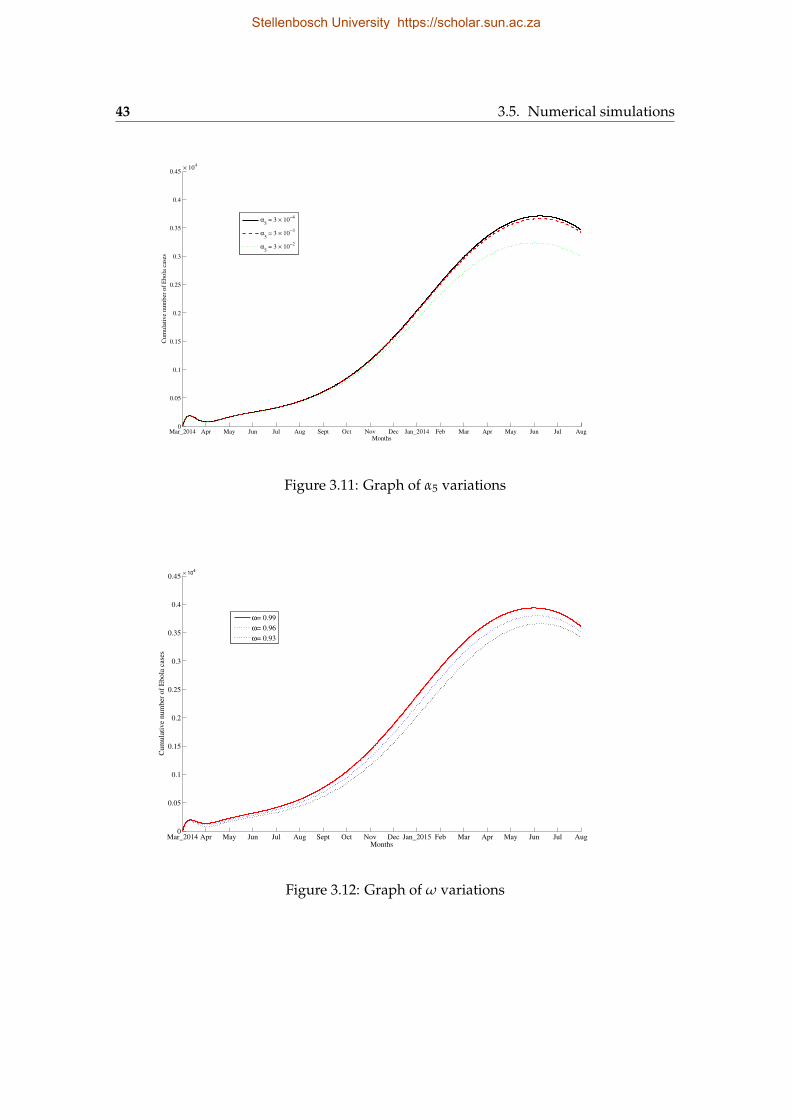
43 3.5. Numerical simulations
Mar_2014 Apr May Jun Jul Aug Sept Oct Nov Dec Jan_2014 Feb Mar Apr May Jun Jul Aug0
0.05
0.1
0.15
0.2
0.25
0.3
0.35
0.4
0.45
Months
Cu
mu
lati
ve
nu
mb
er o
f E
bola
cas
es
α5 = 3 × 10
−4
α5 = 3 × 10
−3
α5 = 3 × 10
−2
× 104
Figure 3.11: Graph of α5 variations
Mar_2014 Apr May Jun Jul Aug Sept Oct Nov Dec Jan_2015 Feb Mar Apr May Jun Jul Aug0
0.05
0.1
0.15
0.2
0.25
0.3
0.35
0.4
0.45
Months
Cum
ula
tive
num
ber
of
Ebola
cas
es
ω= 0.99
ω= 0.96
ω= 0.93
× 104
Figure 3.12: Graph of ω variations
Stellenbosch University https://scholar.sun.ac.za
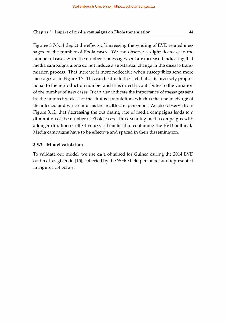
Chapter 3. Impact of media campaigns on Ebola transmission 44
Figures 3.7-3.11 depict the effects of increasing the sending of EVD related mes-sages on the number of Ebola cases. We can observe a slight decrease in thenumber of cases when the number of messages sent are increased indicating thatmedia campaigns alone do not induce a substantial change in the disease trans-mission process. That increase is more noticeable when susceptibles send moremessages as in Figure 3.7. This can be due to the fact that α1 is inversely propor-tional to the reproduction number and thus directly contributes to the variationof the number of new cases. It can also indicate the importance of messages sentby the uninfected class of the studied population, which is the one in charge ofthe infected and which informs the health care personnel. We also observe fromFigure 3.12, that decreasing the out dating rate of media campaigns leads to adiminution of the number of Ebola cases. Thus, sending media campaigns witha longer duration of effectiveness is beneficial in containing the EVD outbreak.Media campaigns have to be effective and spaced in their dissemination.
3.5.3 Model validation
To validate our model, we use data obtained for Guinea during the 2014 EVDoutbreak as given in [15], collected by the WHO field personnel and representedin Figure 3.14 below.
Stellenbosch University https://scholar.sun.ac.za
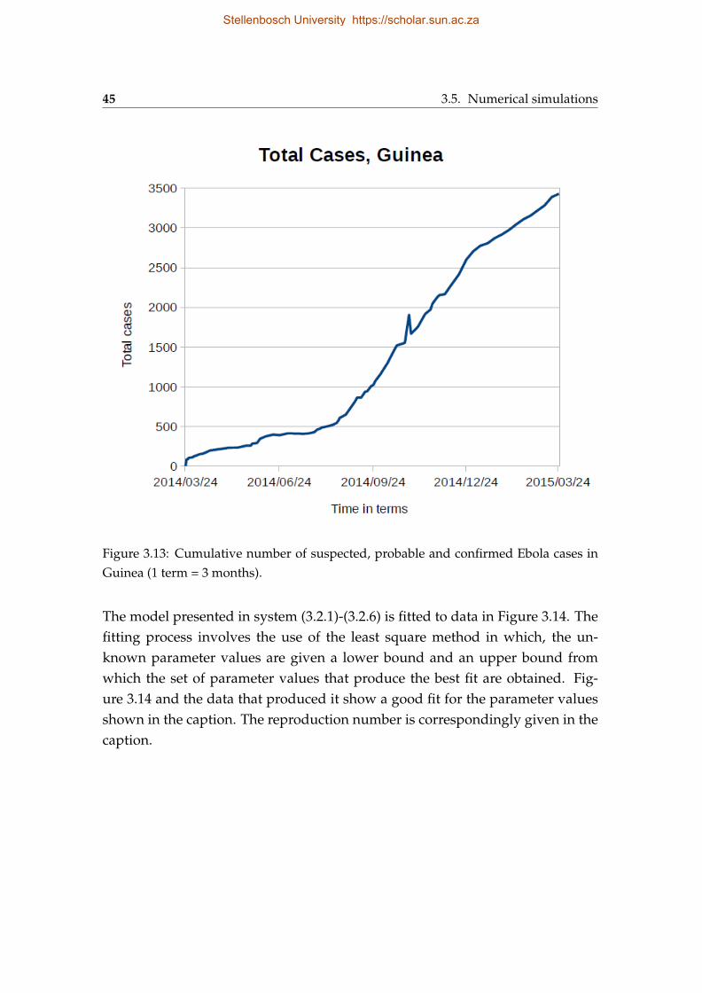
45 3.5. Numerical simulations
Figure 3.13: Cumulative number of suspected, probable and confirmed Ebola cases inGuinea (1 term = 3 months).
The model presented in system (3.2.1)-(3.2.6) is fitted to data in Figure 3.14. Thefitting process involves the use of the least square method in which, the un-known parameter values are given a lower bound and an upper bound fromwhich the set of parameter values that produce the best fit are obtained. Fig-ure 3.14 and the data that produced it show a good fit for the parameter valuesshown in the caption. The reproduction number is correspondingly given in thecaption.
Stellenbosch University https://scholar.sun.ac.za
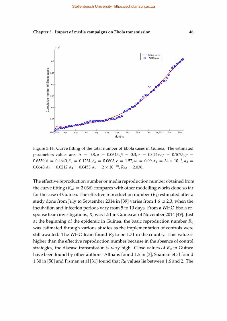
Chapter 3. Impact of media campaigns on Ebola transmission 46
Mar_2014 Apr May Jun July Aug Sept Oct Nov Dec Jan_2015 feb Mar0
0.05
0.1
0.15
0.2
0.25
0.3
Months
Cu
mu
lative
num
ber
of
Ebola
cases
Fitting curve
WHO data
× 104
Figure 3.14: Curve fitting of the total number of Ebola cases in Guinea. The estimatedparameters values are: Λ = 0.8, µ = 0.0643, β = 0.3, σ = 0.0249, γ = 0.1075, p =
0.6559, θ = 0.4640, δ1 = 0.1231, δ2 = 0.0603, c = 1.57, ω = 0.99, α1 = 34× 10−6, α2 =
0.0643, α3 = 0.0212, α4 = 0.0453, α5 = 2× 10⁻¹⁰, RM = 2.036.
The effective reproduction number or media reproduction number obtained fromthe curve fitting (RM = 2.036) compares with other modelling works done so farfor the case of Guinea. The effective reproduction number (Rt) estimated after astudy done from July to September 2014 in [39] varies from 1.6 to 2.3, when theincubation and infection periods vary from 5 to 10 days. From a WHO Ebola re-sponse team investigations, Rt was 1.51 in Guinea as of November 2014 [49]. Justat the beginning of the epidemic in Guinea, the basic reproduction number R0
was estimated through various studies as the implementation of controls werestill awaited. The WHO team found R0 to be 1.71 in the country. This value ishigher than the effective reproduction number because in the absence of controlstrategies, the disease transmission is very high. Close values of R0 in Guineahave been found by other authors. Althaus found 1.5 in [3], Shaman et al found1.30 in [50] and Fisman et al [31] found that R0 values lie between 1.6 and 2. The
Stellenbosch University https://scholar.sun.ac.za
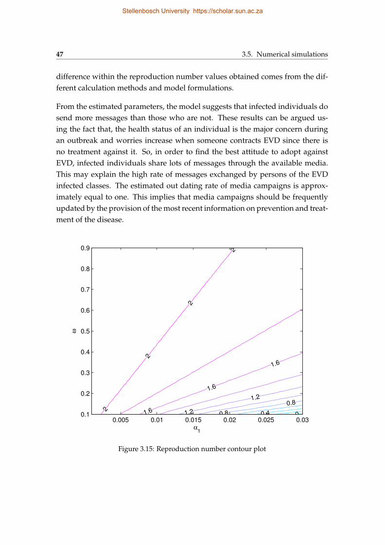
47 3.5. Numerical simulations
difference within the reproduction number values obtained comes from the dif-ferent calculation methods and model formulations.
From the estimated parameters, the model suggests that infected individuals dosend more messages than those who are not. These results can be argued us-ing the fact that, the health status of an individual is the major concern duringan outbreak and worries increase when someone contracts EVD since there isno treatment against it. So, in order to find the best attitude to adopt againstEVD, infected individuals share lots of messages through the available media.This may explain the high rate of messages exchanged by persons of the EVDinfected classes. The estimated out dating rate of media campaigns is approx-imately equal to one. This implies that media campaigns should be frequentlyupdated by the provision of the most recent information on prevention and treat-ment of the disease.
00.4
0.8
0.8
1.2
1.2
1.6
1.6
1.62
2
2
2
α1
ω
0.005 0.01 0.015 0.02 0.025 0.030.1
0.2
0.3
0.4
0.5
0.6
0.7
0.8
0.9
Figure 3.15: Reproduction number contour plot
Stellenbosch University https://scholar.sun.ac.za
Chapter 3. Impact of media campaigns on Ebola transmission 48
The media campaigns reproduction number RM is made of parameters whichdifferently influence its values. The relationship between those parameters canbe evaluated through contour plots. We choose two parameters, α1 and ω, whoseinfluence is clearly significant as shown in Figures 3.7 and 3.12. Figure 3.15shows that α1 largely influences RM when compared to ω. Besides, increasingthe values of α1 decreases RM. Thus, the exchange of EVD related messages iscritical in eradicating an EVD epidemic.
3.6 Conclusion
As a conclusion to this chapter, one can retain that increasing the number of EVDrelated messages produces a slight decrease in the number of EVD cases and me-dia campaigns are more effective when updated. So, the impact of media cam-paigns alone on the disease transmission is not significant. It is therefore neces-sary to implement as well, other control measures against EVD like an eventualtreatment, case-finding or contact tracing in order to limit the disease spread inthe population. This model describes well the dynamics of Ebola virus diseasewhen media campaigns are used as a control measure, but it has its limitationsas well. In fact, people’s reaction to information on a disease is diverse andsometimes doesn’t contribute to the disease eradication. Unexpected behaviourslike unsafe burials or unannounced Ebola cases are still reported in the affectedcommunities during the writing of this thesis. So, the use of an appropriatedfunction better describing the real situation will make this model more realistic.Transmission of Ebola virus disease by asymptomatic individuals is still underinvestigation as of August 2015, and considering it in the transmission processcan result in different disease dynamics. The cost of implementation of controlmeasures is still an issue in the countries affected by Ebola virus disease becauseof their weak economic situation. Thus, in addition to media campaigns, theimplementation of other control measures like educational campaigns, activecase-finding and pharmaceutical interventions should be considered. A con-sideration of those control strategies is best done using optimal control theorywhich is examined in the next chapter.
Stellenbosch University https://scholar.sun.ac.za
Chapter 4
An optimal control model for Ebolavirus disease
4.1 Introduction
The model presented in Chapter 3 does not take into consideration the mostcommonly used strategies in the fight against EVD. These strategies are edu-cational campaigns, active case-finding and pharmaceutical interventions [25].Also the previous model does not explicitly capture mortality due to the disease.In this chapter we incorporate a compartment of the deceased that is importantin disease transmission.
The success of control strategies depends largely on resource mobilisation. Infact, the weak economic situations of most of the EVD affected countries wasa limitation factor in the fight against the disease [37]. So, the use of effectivecontrol measures with minimal cost is observed during an epidemic. Optimalcontrol is best described using mathematical modelling. We formulate a modelfor the optimal control of Ebola virus disease in this chapter.
4.2 Model formulation
Considering a large size and non constant population, we use seven indepen-dent compartments to represent individuals with different disease status. Sus-ceptible individuals (S) are recruited into an heterogeneous population at a rate
49
Stellenbosch University https://scholar.sun.ac.za
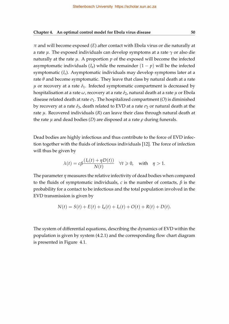
Chapter 4. An optimal control model for Ebola virus disease 50
π and will become exposed (E) after contact with Ebola virus or die naturally ata rate µ. The exposed individuals can develop symptoms at a rate γ or also dienaturally at the rate µ. A proportion p of the exposed will become the infectedasymptomatic individuals (Ia) while the remainder (1− p) will be the infectedsymptomatic (Is). Asymptomatic individuals may develop symptoms later at arate θ and become symptomatic. They leave that class by natural death at a rateµ or recovery at a rate δ1. Infected symptomatic compartment is decreased byhospitalisation at a rate ω, recovery at a rate δ2, natural death at a rate µ or Eboladisease related death at rate σ1. The hospitalized compartment (O) is diminishedby recovery at a rate δ3, death related to EVD at a rate σ2 or natural death at therate µ. Recovered individuals (R) can leave their class through natural death atthe rate µ and dead bodies (D) are disposed at a rate ρ during funerals.
Dead bodies are highly infectious and thus contribute to the force of EVD infec-tion together with the fluids of infectious individuals [12]. The force of infectionwill thus be given by
λ(t) = cβ(Is(t) + ηD(t))
N(t)∀t > 0, with η > 1.
The parameter η measures the relative infectivity of dead bodies when comparedto the fluids of symptomatic individuals, c is the number of contacts, β is theprobability for a contact to be infectious and the total population involved in theEVD transmission is given by
N(t) = S(t) + E(t) + Ia(t) + Is(t) + O(t) + R(t) + D(t).
The system of differential equations, describing the dynamics of EVD within thepopulation is given by system (4.2.1) and the corresponding flow chart diagramis presented in Figure 4.1.
Stellenbosch University https://scholar.sun.ac.za
51 4.2. Model formulation
S
O
R
Is
Ia
E p(1-p)
1
1
2
D
3
2
Figure 4.1: Flow diagram describing EVD dynamics.
4.2.1 Model equations
The system of ordinary differential equations describing the model is given be-low.
dSdt
= π − (λ + µ)S,
dEdt
= λS− (γ + µ)E,
dIa
dt= pγE− (µ + θ + δ1)Ia,
dIs
dt= (1− p)γE + θ Ia − (σ1 + ω + µ + δ2)Is, (4.2.1)
dOdt
= ωIs − (µ + δ3 + σ2)O,
dRdt
= δ1 Ia + δ2 Is + δ3O− µR,
dDdt
= σ1 Is + σ2O− ρD.
Stellenbosch University https://scholar.sun.ac.za
Chapter 4. An optimal control model for Ebola virus disease 52
4.3 Definition and existence of an optimal control
4.3.1 Definition of an optimal control
Stopping the EVD transmission chain is still the main strategy to limit the spreadof the disease. This can be done through educational campaigns which encour-age behavioural changes like safe burial and self isolation [25]. This can also bedone through active case-finding which consists of searching for and recordingcases in the community by talking to local leaders, families or any informants.It significantly helps in limiting further contamination by Ebola virus. Once anindividual is infected by Ebola virus, his chances of recovery can be increasedthrough pharmaceutical interventions which consist of providing intravenousfluid and balancing electrolytes, maintaining oxygen status and blood pressure,treating others infections if they occur [16]. Mathematically, we define three timeseries controls as u1(t), u2(t) and u3(t) for t ∈ [0, T], where T is the time durationof the interventions, to respectively represent the educational campaigns, activecase-finding and pharmaceutical interventions. The implementation of educa-tional campaigns reduces the force of EVD infection which then is modelled bythe expression
λu(t) = cβ(1− u1(t))(Is(t) + ηD(t))
N(t), η > 1.
Active case finding increases the chance of hospitalization and medical care,while pharmaceutical interventions may lead to recovery. The overall objectiveof this chapter, which is to minimize the number of EVD cases and the cost ofcontrol strategies involved, can be mathematically translated into finding piece-wise continuous controls u∗1 , u∗2 , u∗3 and associated state variables S∗, E∗, I∗a , I∗s ,O∗, R∗ and D∗ that minimize the objective functional J given by
J(u1, u2, u3) =∫ T
0
(Is +
α1
2u2
1 +α2
2u2
2 +α3
2u2
3
)(4.3.1)
where αi > 0 for i = 1, 2, 3 are weights associated with the costs of controlprograms.The optimal control problem is thus to minimize the objective functional subject
Stellenbosch University https://scholar.sun.ac.za
53 4.3. Definition and existence of an optimal control
to the system of differential equations (4.3.2).
dSdt
= π − ((1− u1)λ + µ)S,
dEdt
= (1− u1)λS− (γ + µ)E,
dIa
dt= pγE− (µ + θ + δ1)Ia,
dIs
dt= (1− p)γE + θ Ia − (σ1 + u2ω + µ + δ2)Is, (4.3.2)
dOdt
= u2ωIs − (µ + u3δ3 + σ2)O,
dRdt
= δ1 Ia + δ2 Is + u3δ3O− µR,
dDdt
= σ1 Is + σ2O− ρD,
with positive initial conditions defined as S(0) = S0, E(0) = E0, Ia(0) = Ia0, Is(0) =Is0, O(0) = O0, R(0) = R0 and D(0) = D0.
Setting (u∗1 , u∗2 , u∗3) as the optimal controls, the minimization problem can besummarised as
J(u∗1 , u∗2 , u∗3) = min(u1,u2,u3)∈Θ
J(u1, u2, u3) (4.3.3)
where
Θ = (u1, u2, u3)|ui is measurable and 0 ≤ ui(t) ≤ 1 for t ∈ [0, T], i = 1, 2, 3
is the set for the controls.
4.3.2 Invariance and positivity of solutions
The existing solutions of the system (4.3.2) are proven in this subsection to beinvariant and positive.
Theorem 4.3.1. The system (4.3.2) makes biological sense in the region
Φ = (S(t), E(t), Ia(t), Is(t), O(t), R(t), D(t)) ∈ R7 : N(t) 6π
µ
which is attracting and positively invariant with respect to the flow of system (4.3.2).
Stellenbosch University https://scholar.sun.ac.za
Chapter 4. An optimal control model for Ebola virus disease 54
Proof. We assume that µ < ρ within the modelling time. This is reasonable sinceEVD has a higher disease induced death rate when compared to the naturalmortality during the time of an outbreak. By adding all the equations of system(4.3.2) and considering 0 ≤ ui 6 1 for i = 1, 2, 3 we have:
dNdt
6 π − µN. (4.3.4)
Integrating (4.3.4) gives
0 6 N(t) 6(
N(0)− π
µ
)exp(−µt) +
π
µ, ∀ t > 0.
We thus have limt→∞ N(t) <π
µwhen N(0) 6
π
µ. However, if N(0) >
π
µ,
N(t) will decrease toπ
µ. So N(t) is thus a bounded function of time and Φ is
bounded. At limiting equilibrium,
limt→∞
N(t) =π
µ.
Besides, any sum or difference of variables in Φ with positive initial values willremain in Φ or in a neighbourhood of Φ. Thus Φ is positively invariant andattracting with respect to the flow of system (4.3.2).
Theorem 4.3.2. The solutions of our system (4.3.2) are all positive.
Proof. Considering 0 ≤ ui ≤ 1 for i = 1, 2, 3, from system (4.3.2) we have
dSdt
> −(λ(t) + µ)S, ∀ t > 0. (4.3.5)
Solving for (4.3.5) yields
S(t) = S(0) exp[−∫ t
0λ(τ) dτ − µt
]which is positive given that S(0) is also positive. From (4.3.2) we also have
dEdt
> −(γ + µ)E ∀ t > 0,
so thatE(t) = E(0) exp[−(γ + µ)]t ∀ t ≥ 0.
Stellenbosch University https://scholar.sun.ac.za
55 4.3. Definition and existence of an optimal control
So E(t) is positive given its positive initial conditions.The third equation of system (4.3.2) yields
dIa
dt> −(µ + θ + δ1)Ia ∀ t > 0
from whichIa(t) = Ia(0) exp[−(µ + θ + δ1)]t.
Thus,Ia(t) > Ia(0) exp[−(µ + θ + δ1)]t ∀ t ≥ 0
and Ia(t) is positive since Ia(0) is also positive. The remaining equations yield
Is(t) > Is(0) exp[−(µ + σ1 + ω + δ2)]t ∀ t ≥ 0,
O(t) > O(0) exp[−(µ + σ2 + δ3)]t ∀ t ≥ 0,
R(t) > R(0) exp(−µt) ∀ t ≥ 0,
D(t) > D(0) exp(−ρt) ∀ t ≥ 0.
So Ia(t), Is(t), O(t), R(t) and D(t) are all positive for positive initial conditions.Thus all the state variables are positive.
4.3.3 Existence of an optimal control
The existence of an optimal control is given in Theorem 4.1 formulated by Flem-ing and Rihel in [41] as follows:
Theorem 4.3.3. Consider the control problem with system (4.3.2). There exists u∗ =(u∗1 , u∗2 , u∗3) ∈ Θ such that:
J(u∗1 , u∗2 , u∗3) = min(u1,u2,u3)∈Θ
J(u1, u2, u3).
Proof. Conditions for the optimal control to exist are the following:
(i) The set of controls and corresponding state variables, denoted Ω, is nonempty.From Theorem 9.2.1 of Lukes in [36], the solutions of system (4.3.2) exist.Thus, the set Ω is non empty.
Stellenbosch University https://scholar.sun.ac.za
Chapter 4. An optimal control model for Ebola virus disease 56
(ii) The set Θ is convex and closed.The set Θ is closed by definition. Given (θ1, θ2) ∈ Θ2 and t ∈ [0, 1] suchthat θ1 = (u11, u21, u31) and θ2 = (u12, u22, u32), the line tθ1 + (1− t)θ2 =
(tu11 + (1 − t)u12, tu21 + (1 − t)u22, tu31 + (1 − t)u32) belongs to Θ sinceeach of its components is in between zero and one. Thus Θ is convex.
(iii) The right hand side of the state system (4.3.2) is bounded by a linear func-tion in the state and control variables.System (4.3.2) is linear with respect to u1 and u2. Besides, its solutions areabsolutely continuous [36], which implies that they are bounded and state-ment (iii) is then satisfied.
(iv) The integrand of the objective functional (4.3.1) is concave on Θ.The integrand L of the objective functional is given by
L(Is, u1, u2, u3) = Is +α1
2u2
1 +α2
2u2
2 +α3
2u2
3.
Given (θ1, θ2) ∈ Θ2 and t ∈ [0, 1] such that θ1 = (u11, u21, u31), θ2 =
(u12, u22, u32) and tθ1 +(1− t)θ2 = (tu11 +(1− t)u12, tu21 +(1− t)u22, tu31 +
(1− t)u32).
L(tθ1 + (1− t)θ2) = Is +α1
2(tu11 + (1− t)u12)
2
+α2
2(tu21 + (1− t)u22)
2 +α3
2(tu31 + (1− t)u32)
2
and
tL(θ1) + (1− t)L(θ2) = Is +α1
2(tu2
11 + (1− t)u212)
+α2
2(tu2
21 + (1− t)u222) +
α3
2(tu2
31 + (1− t)u232).
Since
(tu11 + (1− t)u12)2 > (tu2
11 + (1− t)u212),
(tu21 + (1− t)u22)2 > (tu2
21 + (1− t)u222),
(tu31 + (1− t)u32)2 > (tu2
31 + (1− t)u232)
for any (θ1, θ2) ∈ Θ2 and t ∈ [0, 1], L(tθ1 + (1 − t)θ2) ≥ tL(θ1) + (1 −t)L(θ2) which thus proves that L is concave.
Stellenbosch University https://scholar.sun.ac.za
57 4.4. Analysis of optimal control
(v) There exist constants η1, η2 > 0 and σ > 1 such that the integrand L of theobjective functional satisfies
L(Is, u1, u2, u3) ≤ η1 + η2(|u1|2 + |u2|2 + |u3|2)σ/2.
Since Is is bounded (see [36]), there exists a constant η1 > 0 such that Is ≤ η1
and setting η2 = maxi=1,2,3 αi we obtain L(Is, u1, u2, u3) ≤ η1 + η2(|u1|2 +|u2|2 + |u3|2) with σ = 2. So, condition (v) is satisfied and the optimal-ity system (4.3.1), (4.3.2) and (4.3.3) has a solution which is unique for Tsufficiently small [34].
4.4 Analysis of optimal control
The optimality system (4.3.1), (4.3.2) and (4.3.3) can be converted into a problemof minimizing a pointwise Hamiltonian H with respect to u1, u2, u3 thanks to thePontryagin’s Maximum Principle (PMP) in [18]. The Hamiltonian is given by
H = Is +α1
2u2
1 +α2
2u2
2 +α3
2u2
3 +7
∑i=0
ξigi,
where gi is the ith right hand side of system (4.3.2) and ξi is the ith adjoint. Wethus have the following results.
Theorem 4.4.1. There exist an optimal control triplet (u∗1 , u∗2 , u∗3) and correspond-ing state solutions S∗, E∗, I∗a , I∗s , O∗, R∗ and D∗ that minimize J(u1, u2, u3) over Θ.
Stellenbosch University https://scholar.sun.ac.za
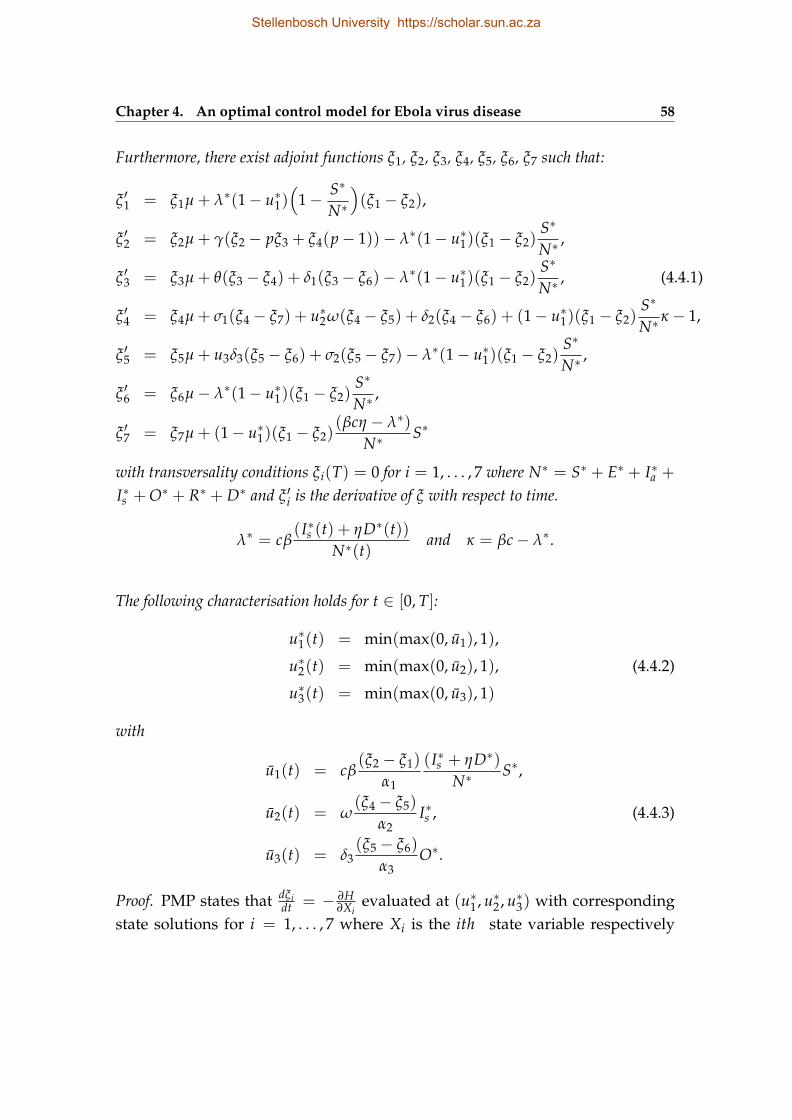
Chapter 4. An optimal control model for Ebola virus disease 58
Furthermore, there exist adjoint functions ξ1, ξ2, ξ3, ξ4, ξ5, ξ6, ξ7 such that:
ξ ′1 = ξ1µ + λ∗(1− u∗1)(
1− S∗
N∗)(ξ1 − ξ2),
ξ ′2 = ξ2µ + γ(ξ2 − pξ3 + ξ4(p− 1))− λ∗(1− u∗1)(ξ1 − ξ2)S∗
N∗,
ξ ′3 = ξ3µ + θ(ξ3 − ξ4) + δ1(ξ3 − ξ6)− λ∗(1− u∗1)(ξ1 − ξ2)S∗
N∗, (4.4.1)
ξ ′4 = ξ4µ + σ1(ξ4 − ξ7) + u∗2ω(ξ4 − ξ5) + δ2(ξ4 − ξ6) + (1− u∗1)(ξ1 − ξ2)S∗
N∗κ − 1,
ξ ′5 = ξ5µ + u3δ3(ξ5 − ξ6) + σ2(ξ5 − ξ7)− λ∗(1− u∗1)(ξ1 − ξ2)S∗
N∗,
ξ ′6 = ξ6µ− λ∗(1− u∗1)(ξ1 − ξ2)S∗
N∗,
ξ ′7 = ξ7µ + (1− u∗1)(ξ1 − ξ2)(βcη − λ∗)
N∗S∗
with transversality conditions ξi(T) = 0 for i = 1, . . . , 7 where N∗ = S∗ + E∗ + I∗a +
I∗s + O∗ + R∗ + D∗ and ξ ′i is the derivative of ξ with respect to time.
λ∗ = cβ(I∗s (t) + ηD∗(t))
N∗(t)and κ = βc− λ∗.
The following characterisation holds for t ∈ [0, T]:
u∗1(t) = min(max(0, u1), 1),
u∗2(t) = min(max(0, u2), 1), (4.4.2)
u∗3(t) = min(max(0, u3), 1)
with
u1(t) = cβ(ξ2 − ξ1)
α1
(I∗s + ηD∗)N∗
S∗,
u2(t) = ω(ξ4 − ξ5)
α2I∗s , (4.4.3)
u3(t) = δ3(ξ5 − ξ6)
α3O∗.
Proof. PMP states that dξidt = − ∂H
∂Xievaluated at (u∗1 , u∗2 , u∗3) with corresponding
state solutions for i = 1, . . . , 7 where Xi is the ith state variable respectively
Stellenbosch University https://scholar.sun.ac.za
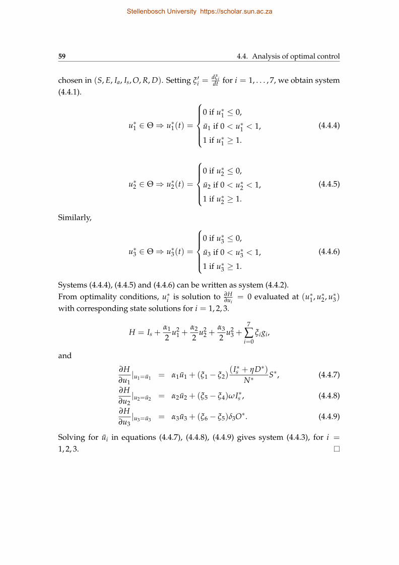
59 4.4. Analysis of optimal control
chosen in (S, E, Ia, Is, O, R, D). Setting ξ ′i =dξidt for i = 1, . . . , 7, we obtain system
(4.4.1).
u∗1 ∈ Θ⇒ u∗1(t) =
0 if u∗1 ≤ 0,
u1 if 0 < u∗1 < 1,
1 if u∗1 ≥ 1.
(4.4.4)
u∗2 ∈ Θ⇒ u∗2(t) =
0 if u∗2 ≤ 0,
u2 if 0 < u∗2 < 1,
1 if u∗2 ≥ 1.
(4.4.5)
Similarly,
u∗3 ∈ Θ⇒ u∗3(t) =
0 if u∗3 ≤ 0,
u3 if 0 < u∗3 < 1,
1 if u∗3 ≥ 1.
(4.4.6)
Systems (4.4.4), (4.4.5) and (4.4.6) can be written as system (4.4.2).From optimality conditions, u∗i is solution to ∂H
∂ui= 0 evaluated at (u∗1 , u∗2 , u∗3)
with corresponding state solutions for i = 1, 2, 3.
H = Is +α1
2u2
1 +α2
2u2
2 +α3
2u2
3 +7
∑i=0
ξigi,
and
∂H∂u1|u1=u1 = α1u1 + (ξ1 − ξ2)
(I∗s + ηD∗)N∗
S∗, (4.4.7)
∂H∂u2|u2=u2 = α2u2 + (ξ5 − ξ4)ωI∗s , (4.4.8)
∂H∂u3|u3=u3 = α3u3 + (ξ6 − ξ5)δ3O∗. (4.4.9)
Solving for ui in equations (4.4.7), (4.4.8), (4.4.9) gives system (4.4.3), for i =
1, 2, 3.
Stellenbosch University https://scholar.sun.ac.za
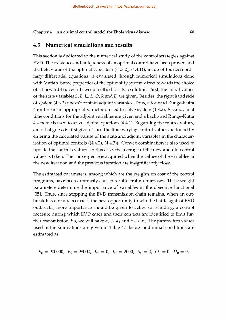
Chapter 4. An optimal control model for Ebola virus disease 60
4.5 Numerical simulations and results
This section is dedicated to the numerical study of the control strategies againstEVD. The existence and uniqueness of an optimal control have been proven andthe behaviour of the optimality system ((4.3.2), (4.4.1)), made of fourteen ordi-nary differential equations, is evaluated through numerical simulations donewith Matlab. Some properties of the optimality system direct towards the choiceof a Forward-Backward sweep method for its resolution. First, the initial valuesof the state variables S, E, Ia, Is, O, R and D are given. Besides, the right hand sideof system (4.3.2) doesn’t contain adjoint variables. Thus, a forward Runge-Kutta4 routine is an appropriated method used to solve system (4.3.2). Second, finaltime conditions for the adjoint variables are given and a backward Runge-Kutta4 scheme is used to solve adjoint equations (4.4.1). Regarding the control values,an initial guess is first given. Then the time varying control values are found byentering the calculated values of the state and adjoint variables in the character-isation of optimal controls ((4.4.2), (4.4.3)). Convex combination is also used toupdate the controls values. In this case, the average of the new and old controlvalues is taken. The convergence is acquired when the values of the variables inthe new iteration and the previous iteration are insignificantly close.
The estimated parameters, among which are the weights on cost of the controlprograms, have been arbitrarily chosen for illustration purposes. These weightparameters determine the importance of variables in the objective functional[35]. Thus, since stopping the EVD transmission chain remains, when an out-break has already occurred, the best opportunity to win the battle against EVDoutbreaks, more importance should be given to active case-finding, a controlmeasure during which EVD cases and their contacts are identified to limit fur-ther transmission. So, we will have α2 > α1 and α2 > α3. The parameters valuesused in the simulations are given in Table 4.1 below and initial conditions areestimated as:
S0 = 900000, E0 = 98000, Ia0 = 0, Is0 = 2000, R0 = 0, O0 = 0, D0 = 0.
Stellenbosch University https://scholar.sun.ac.za
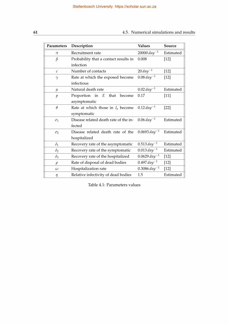
61 4.5. Numerical simulations and results
Parameters Description Values Source
π Recruitment rate 20000 day−1 Estimated
β Probability that a contact results ininfection
0.008 [12]
c Number of contacts 20 day−1 [12]
γ Rate at which the exposed becomeinfectious
0.08 day−1 [12]
µ Natural death rate 0.02 day−1 Estimated
p Proportion in E that becomeasymptomatic
0.17 [11]
θ Rate at which those in Ia becomesymptomatic
0.12 day−1 [22]
σ1 Disease related death rate of the in-fected
0.06 day−1 Estimated
σ2 Disease related death rate of thehospitalized
0.0693 day−1 Estimated
δ1 Recovery rate of the asymptomatic 0.513 day−1 Estimated
δ2 Recovery rate of the symptomatic 0.013 day−1 Estimated
δ3 Recovery rate of the hospitalized 0.0629 day−1 [12]
ρ Rate of disposal of dead bodies 0.497 day−1 [12]
ω Hospitalization rate 0.3086 day−1 [12]
η Relative infectivity of dead bodies 1.5 Estimated
Table 4.1: Parameters values
Stellenbosch University https://scholar.sun.ac.za
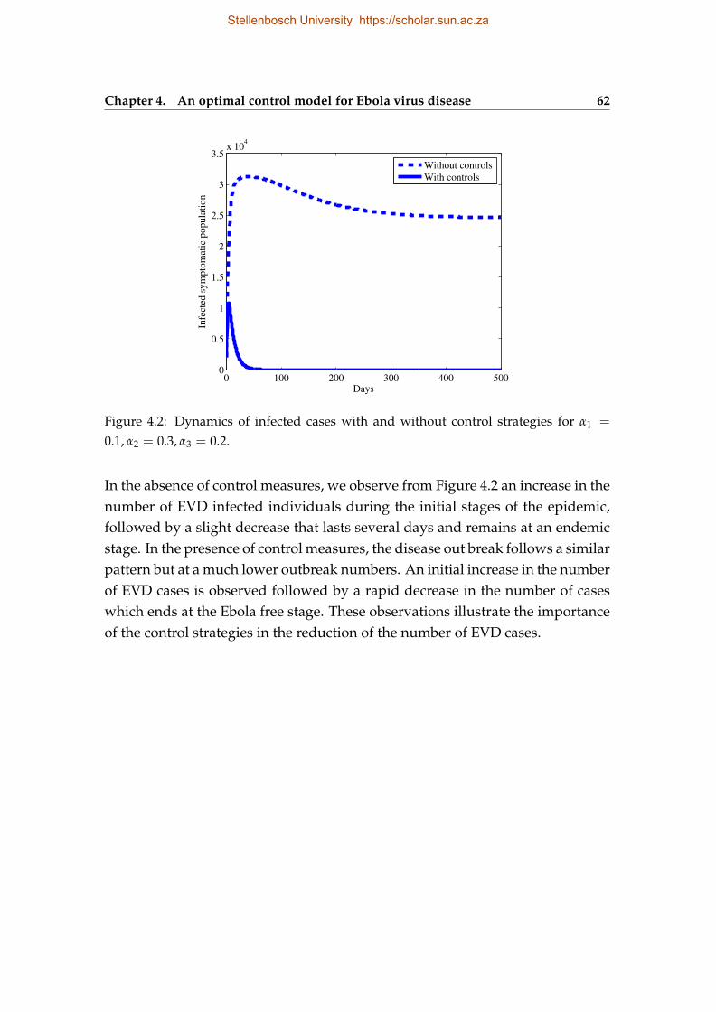
Chapter 4. An optimal control model for Ebola virus disease 62
0 100 200 300 400 5000
0.5
1
1.5
2
2.5
3
3.5x 10
4
Days
Infe
cted
sy
mp
tom
atic
po
pu
lati
on
Without controls
With controls
Figure 4.2: Dynamics of infected cases with and without control strategies for α1 =
0.1, α2 = 0.3, α3 = 0.2.
In the absence of control measures, we observe from Figure 4.2 an increase in thenumber of EVD infected individuals during the initial stages of the epidemic,followed by a slight decrease that lasts several days and remains at an endemicstage. In the presence of control measures, the disease out break follows a similarpattern but at a much lower outbreak numbers. An initial increase in the numberof EVD cases is observed followed by a rapid decrease in the number of caseswhich ends at the Ebola free stage. These observations illustrate the importanceof the control strategies in the reduction of the number of EVD cases.
Stellenbosch University https://scholar.sun.ac.za
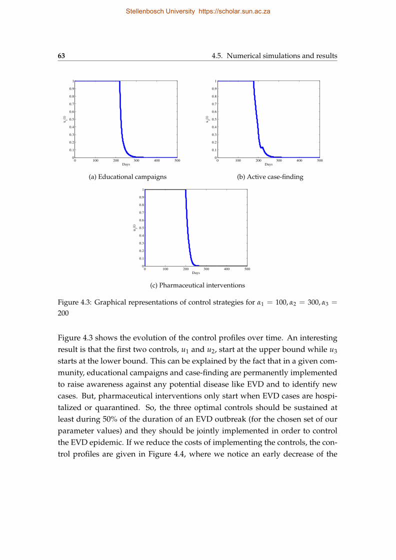
63 4.5. Numerical simulations and results
0 100 200 300 400 5000
0.1
0.2
0.3
0.4
0.5
0.6
0.7
0.8
0.9
1
Days
u1(t)
(a) Educational campaigns
0 100 200 300 400 5000
0.1
0.2
0.3
0.4
0.5
0.6
0.7
0.8
0.9
1
Days
u2(t)
(b) Active case-finding
0 100 200 300 400 5000
0.1
0.2
0.3
0.4
0.5
0.6
0.7
0.8
0.9
1
Days
u3(t)
(c) Pharmaceutical interventions
Figure 4.3: Graphical representations of control strategies for α1 = 100, α2 = 300, α3 =
200
Figure 4.3 shows the evolution of the control profiles over time. An interestingresult is that the first two controls, u1 and u2, start at the upper bound while u3
starts at the lower bound. This can be explained by the fact that in a given com-munity, educational campaigns and case-finding are permanently implementedto raise awareness against any potential disease like EVD and to identify newcases. But, pharmaceutical interventions only start when EVD cases are hospi-talized or quarantined. So, the three optimal controls should be sustained atleast during 50% of the duration of an EVD outbreak (for the chosen set of ourparameter values) and they should be jointly implemented in order to controlthe EVD epidemic. If we reduce the costs of implementing the controls, the con-trol profiles are given in Figure 4.4, where we notice an early decrease of the
Stellenbosch University https://scholar.sun.ac.za
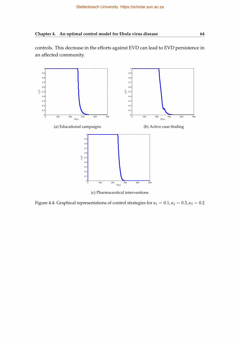
Chapter 4. An optimal control model for Ebola virus disease 64
controls. This decrease in the efforts against EVD can lead to EVD persistence inan affected community.
0 100 200 300 400 5000
0.1
0.2
0.3
0.4
0.5
0.6
0.7
0.8
0.9
1
Days
u1(t)
(a) Educational campaigns
0 100 200 300 400 5000
0.1
0.2
0.3
0.4
0.5
0.6
0.7
0.8
0.9
1
Days
u2(t)
(b) Active case-finding
0 100 200 300 400 5000
0.1
0.2
0.3
0.4
0.5
0.6
0.7
0.8
0.9
1
Days
u3(t)
(c) Pharmaceutical interventions
Figure 4.4: Graphical representations of control strategies for α1 = 0.1, α2 = 0.3, α3 = 0.2
Stellenbosch University https://scholar.sun.ac.za
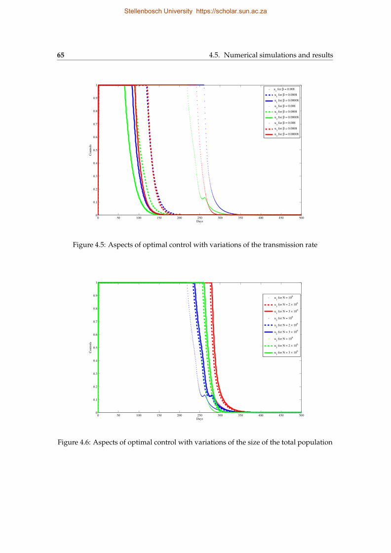
65 4.5. Numerical simulations and results
0 50 100 150 200 250 300 350 400 450 5000
0.1
0.2
0.3
0.4
0.5
0.6
0.7
0.8
0.9
1
Days
Contr
ols
u1 for β = 0.008
u1 for β = 0.0008
u1 for β = 0.00008
u2 for β = 0.008
u2 for β = 0.0008
u2 for β = 0.00008
u3 for β = 0.008
u3 for β = 0.0008
u3 for β = 0.00008
Figure 4.5: Aspects of optimal control with variations of the transmission rate
0 50 100 150 200 250 300 350 400 450 5000
0.1
0.2
0.3
0.4
0.5
0.6
0.7
0.8
0.9
1
Days
Contr
ols
u1 for N = 10
6
u1 for N = 2 × 10
6
u1 for N = 3 × 10
6
u2 for N = 10
6
u2 for N = 2 × 10
6
u2 for N = 3 × 10
6
u3 for N = 10
6
u3 for N = 2 × 10
6
u3 for N = 3 × 10
6
Figure 4.6: Aspects of optimal control with variations of the size of the total population
Stellenbosch University https://scholar.sun.ac.za
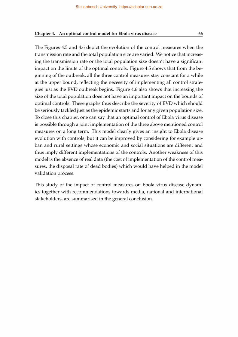
Chapter 4. An optimal control model for Ebola virus disease 66
The Figures 4.5 and 4.6 depict the evolution of the control measures when thetransmission rate and the total population size are varied. We notice that increas-ing the transmission rate or the total population size doesn’t have a significantimpact on the limits of the optimal controls. Figure 4.5 shows that from the be-ginning of the outbreak, all the three control measures stay constant for a whileat the upper bound, reflecting the necessity of implementing all control strate-gies just as the EVD outbreak begins. Figure 4.6 also shows that increasing thesize of the total population does not have an important impact on the bounds ofoptimal controls. These graphs thus describe the severity of EVD which shouldbe seriously tackled just as the epidemic starts and for any given population size.To close this chapter, one can say that an optimal control of Ebola virus diseaseis possible through a joint implementation of the three above mentioned controlmeasures on a long term. This model clearly gives an insight to Ebola diseaseevolution with controls, but it can be improved by considering for example ur-ban and rural settings whose economic and social situations are different andthus imply different implementations of the controls. Another weakness of thismodel is the absence of real data (the cost of implementation of the control mea-sures, the disposal rate of dead bodies) which would have helped in the modelvalidation process.
This study of the impact of control measures on Ebola virus disease dynam-ics together with recommendations towards media, national and internationalstakeholders, are summarised in the general conclusion.
Stellenbosch University https://scholar.sun.ac.za
Chapter 5
General conclusion
The overall objective of this research project was to evaluate the impact of im-plemented control measures on Ebola disease evolution. First, a compartmentalmodel comprising of individuals with different EVD infection status, who sendEVD related messages through media was drawn and the role of media cam-paigns on EVD transmission was analysed through the model. The effects ofmedia campaigns on people’s behaviour was represented by a reduction factorwhich decreased the number of new EVD cases. Stability analysis was presentedin terms of the model reproduction number RM. It was shown that the diseasefree and the endemic equilibria are locally stable if RM < 1 and RM > 1 respec-tively. The inclusion of the asymptomatic infected class resulted in the modelexhibiting a backward bifurcation, emphasizing thus the necessity of intense ef-forts against EVD as a result of undetected asymptomatic cases. The existenceof a backward bifurcation has important implications in the design of policiesand strategies to eradicate or control an epidemic. In the presence of a back-ward bifurcation, classical policies on disease eradication need to be changed asEVD can persist even when the threshold parameter RM, is less than one. Wechose data from Guinea, the country where this 2014 Ebola outbreak started,to validate this model. The model was fitted to the data from the CDC web-site [15]. The fitting process was successful and the parameter values generatedthrough it yielded an RM value of 2.036. The value of the reproduction numbercompares very well with values obtained by other researchers, see for instance[3, 39]. The model evaluated the impact of media campaigns on the reduction ofthe number of Ebola cases through numerical simulations and we have observed
67
Stellenbosch University https://scholar.sun.ac.za
Chapter 5. General conclusion 68
a decrease in the prevalence of the disease when media campaigns were used ascontrol strategy. This first model is not without shortcomings. The reaction tomedia campaigns by individuals doesn’t always lead to a reduction in the num-ber of future contaminations. So, a function representing the influence of mediacampaigns on individuals’ behaviour and which takes into account the differentcultural settings would be an innovative and informative addition to this model.Aspects of quarantine, contact tracing and case identification initiatives are pos-sible additions that can make this model more reliable.
Second, an optimal control of Ebola disease was described by a seven com-partments deterministic model, obtained by extending the previous one to hos-pitalized and dead individuals. They were considered together with educa-tional campaigns, active case-finding and pharmaceutical interventions as con-trol strategies implemented to limit the number of individuals entering the ex-posed and dead classes. The existence of an optimal control set was proven andits analysis was done using Pontryagin’s Maximum Principle. The simulationsresults showed that optimal control of Ebola virus disease is doable througheducational campaigns, active case-finding and pharmaceutical interventions.They showed as well that a long term support for the joint implementation ofthose control strategies was needed for better results. The variation of the totalpopulation size indicated that independent of the size of the population, inter-ventions against any Ebola disease outbreak should begin at the onset of theepidemic for rapid and effective control. This second model of Ebola disease isnot without limits as well. The weights on cost considered here are for illustra-tive purposes. More realistic results will be obtained if real data on the cost of theimplementation of control strategies are used. One of the challenges here is thefact that the 2014 Ebola outbreak is still ongoing during the writing of the thesisand only partial data on the cost of the disease eradication are available. Oncethe epidemic will be declared over, statistics on its burden will be available and abetter cost-effectiveness of the disease will be obtained. Another shortcoming ofthis model is the estimated value of the rate of disposal of dead bodies. Unsafeburials of Ebola related dead individuals are still denounced in countries likeGuinea, and that makes it difficult to find the exact number of Ebola deaths andthe rate at which they are buried. Despite the shortcomings, these models still
Stellenbosch University https://scholar.sun.ac.za
69
provide some useful insights into the control of EVD through the implementa-tion of the discussed control measures.
The study done in this thesis recommends a better collaboration between healthauthorities and media for an early announcement of any epidemic, frequent up-dates of informations sent by media related to Ebola disease, a joint implemen-tation of all the control strategies studied, the provision of sufficient financialresources for a sustained implementation of the control measures by nationaland international organisations.
These models can be extended by considering rural and urban settings sepa-rately, where the implementation of controls is not done at the same scale. Cul-tural beliefs are deeply anchored in people’s behaviours in rural settings andchanging of habits as prescribed by health care givers is therefore more difficult.So, the choice of the control strategies, which take into account the realities ofthe affected countries remains the best option in the fight against Ebola virusdisease. Since the transmission of Ebola disease by asymptomatic infected indi-viduals is still being investigated at the time of writing this thesis, considering itin a future Ebola disease dynamics model can be an innovation as well.
Stellenbosch University https://scholar.sun.ac.za
List of references
[1] Centers for Disease Control and Prevention. Review of human-to-humantransmission of Ebola virus. 2015. http://www.cdc.gov/vhf/ebola/
transmission/human-transmission.html#3 (accessed on August 3, 2015).
[2] E. M. Leroy, S. Baize, V. E. Volchkov, S. P. Fisher-Hoch, M-C Georges-Courbot, J. Lansoud-Soukate, M. Capron, P. debré, J. B. McCormick and A.J. Georges. Human asymptomatic Ebola infection and strong inflammatoryresponse. The Lancet, 355:2210–2215, 2000.
[3] C. L. Althaus. Estimating the reproduction number of Ebola virus (EBOV)during the 2014 outbreak in West Africa. Plos Current Outbreaks, 2014, DOI:10.1371/currents.outbreaks.91afb5e0f279e7f29e7056095255b288.
[4] A. G. Baxter. Symptomless infection with Ebola virus. The Lancet,355(9222):2178–2179, 2014.
[5] S. L. Coyle, R. F. Boruch and C. F. Turner. Evaluating AIDS prevention pro-grams: expanded edition. National Academies Press, 1991.
[6] C. Castilho. Optimal control of an epidemic through educational cam-paigns. Electronic Journal of Differential Equations, 2006(125):1–11, 2006.
[7] C. Castillo-Chavez and B. Song. Dynamical models of tuberculosis and theirapplications. Mathematical Bioscience and Engeneering, 1(2):361–404, 2004.
[8] G. Chowell and H. Nishiura. Transmission dynamics and control of Ebolavirus disease (EVD): a review. BMC Medicine, 12(193), 2014. http://www.
biomedcentral.com/1741-7015/12/196 (accessed in February 2015).
i
Stellenbosch University https://scholar.sun.ac.za
List of references ii
[9] M. I. Meltzer, C. Y. Atkins, S. Santibanez, B. Knust, B. W. Peterson, E. D.Ervin, S. T. Nichol, I. K. Damon and M. L. Washington. Estimating thefuture number of cases in the Ebola epidemic - Liberia and Sierra Leone,2014-2015. Morbidity and Mortality Weekly Report, 63(03):1–14, 2014.
[10] P. V. D. Driessche and J. Watmough. Reproduction numbers and sub-threshold endemic equilibria for compartmental models of disease trans-mission. Mathematical Biosciences, 180(2002):29–48, 2002.
[11] S. E. Bellan, J. R. C. Pulliam, J. Dushoff and L. A. Meyers. Ebola con-trol: effect of asymptomatic infection and acquired immunity. The Lancet,384(9953):1499–1500, 2014.
[12] C. M. Rivers, E. T. Logfren, M. Marathe, S. Eubank and B. L. Lewis.Modeling the impact of interventions on an epidemic of Ebola in SierraLeone and Liberia. Plos Current Outbreaks, 2014, DOI: 10.1371/cur-rents.outbreaks.4d41fe5d6c05e9df30ddce33c66d084c.
[13] H. Feldmann and T. W. Geisbert. Ebola haemorrhagic fever. Lancet, 387:849–862, 2011.
[14] Centers for Disease Control and Prevention. 2014 Ebola outbreak in WestAfrica - case counts. 2015. http://www.cdc.gov/vhf/ebola/outbreaks/
2014-west-africa/case-counts.html (accessed in April 2015).
[15] Centers for Disease Control and Prevention. 2014 Ebola outbreak in WestAfrica - reported cases graphs. 2015. http://www.cdc.gov/vhf/ebola/
outbreaks/2014-west-africa/cumulative-cases-graphs.html (accessedin April 2015).
[16] Centers for Disease Control and Prevention. Treatment. 2015. http://www.cdc.gov/vhf/ebola/treatment/index.html (accessed in February 2015).
[17] Centers for Disease Control and Prevention. Why Ebola is not likely tobecome airborne. 2015. http://www.cdc.gov/vhf/ebola/pdf/mutations.
pdf (accessed on June 2, 2015).
[18] L. S. Pontryagin, V. G. Boltyanskii, R. V. Gamkrelidze and E. F. Mishchenko.The mathematical theory of optimal processes. Interscience Publishers, 1962.
Stellenbosch University https://scholar.sun.ac.za
iii List of references
[19] T. W. Geisbert and L. E. Hensley. Ebola virus: new insights into disease ae-tiopathology and possible therapeutic interventions. Expertreviews in Molec-ular Medecine, 6, 2004, DOI: 10.1017/S1462399404008300.
[20] S. Lee, M. Golinsky and G. Chowell. Modelling optimal age-specific vacci-nation strategies against pandemic Influenza. Bulletin of Mathematical Biol-ogy, 2011, DOI: 10.1007/s11538-011-9704-y.
[21] Google. Google play- about Ebola. 2014. https://play.google.com/
store/apps/details?id=cc.snapp.aboutebola&hl=en (accessed in De-cember 2014).
[22] C. N. Haas. On the quarantine period for Ebolavirus. Plos Current Outbreaks, 2014, DOI: 10.1371/cur-rents.outbreaks.2ab4b76ba7263ff0f084766e43abbd89.
[23] K. P. Hadeler and P. V. D. Driessche. Backward bifurcation in epidemic con-trol. Elsevier, 1997. http://www.uvm.edu/~pdodds/files/papers/others/
everything/hadeler1997a.pdf (accessed in March 2015).
[24] World Health Organization. Case definition recommendations for Ebolaor Marburg virus diseases. 2014. http://www.afro.who.int (accessed inDecember 2014).
[25] World Health Organization. Ebola and Marburg virus disease epi-demics: preparedness, alert, control and evaluation. 2014, WHO/H-SE/PED/CED/2014.05.
[26] World Health Organization. Ebola vaccines, therapies and dignostics.2015. http://www.who.int/medicines/emp_ebola_q_as/en/ (accessed onMay 30, 2015).
[27] G. j. Rubin, H.W.W Potts and S. Michie. The impact of communicationsabout swine flu (influenza A H1N1v) on public responses to the outbreak:results from 36 national telephone surveys in the UK. Health TechnologyAssessment, 14(34):183–266, 2010.
Stellenbosch University https://scholar.sun.ac.za
List of references iv
[28] A. Pandey, k. E. Atkins, j. Medlock, N. wenzel, J. P. Townsend, J. E. Childs, T.G. Nyenswah, M. L. Ndeffo-Mbah and A. P. Galvani. Strategies for containgEbola in West Africa. Sciencexpress, 346(6212):991–995, 2014.
[29] T. K. Kar and S. Jana. A theoretical study on mathematical modellingof an infectious disease with application of optimal control. BioSystems,11(2013):37–50, 2012.
[30] J. J. Muyembe, S. Mulanga, J. Masumu, A. Kemp and J. T. Paweska. Ebolavirus outbreaks in Africa: past and present. Onderstepoort Journal of Veteri-nary Research, 79(2), 2012.
[31] D. Fisman , E. Khoo and A. Tuite. Early epidemics of the WestAfrican 2014 Ebola outbreak: estimates derived with a simple two-parameter model. Plos Currents Outbreaks, 6, 2014, DOI: 10.1371/cur-rents.outbreaks.89c0d3783f36958d96ebbae97348d571.
[32] The Lancet’s free Ebola resource centre. The medium and the message ofEbola. The Lancet, 384(9955):1641, 2014.
[33] E. Jung, S. Lenhart and Z. Feng. Optimal control of treatments in a two-strain tuberculosis model. Discrete and Continuous Dynamical Systems-seriesB, 2(4):473–482, 2002.
[34] K. R. Fister, S. Lenhart and J. S. McNally. Optimizing chemotherapy in anHIV model. Electronic Journal of Differential Equations, 1998(32):1–12, 1998.
[35] S. Lenhart and J. T. Workman. Optimal controls applied to biological models.Chapman and Hall/CRC, 2007.
[36] D. L. Lukes. Differential equations: classical to controlled. Academic Press,1982.
[37] Nature. Six challenges to stamping out Ebola. 2015. http://www.nature.
com/news/six-challenges-to-stamping-out-ebola-1.16964 (accessed inMay 2015).
[38] K. A. Pawelek, A. Oeldorf-Hirsch and L. Rong. Modeling the impact ofTwitter on influenza epidemics. Mathematical Bioscience and Engeneering,11(6):1337–1356, 2014.
Stellenbosch University https://scholar.sun.ac.za
v List of references
[39] S. Towers, O. Patterson-lomba and C. Castillo-Chavez. Temporal vari-ations in the effective reproduction number of the 2014 West AfricaEbola outbreak. Plos Current Outbreaks, 2014, DOI: 10.1371/cur-rents.outbreaks.9e4c4294ec8ce1adad283172b16bc908.
[40] A. Rachab and D. F. M. Torres. Mathematical modelling, simulation andoptimal control of the 2014 Ebola outbreak in West Africa. Discrete Dynamicsin Nature and Society, 2015:9, 2015.
[41] Fleming, H. Wendell, Rishel and W. Raymond. Deterministic and stochasticoptimal control, volume 1. Springer-Verlag, 1975.
[42] J. Astacio, D. Briere, M. Guillén, J. Martínez, F. Rodriguez andN. Valuenzuela-Campos. Mathematical models to study the outbreaks ofEbola. https://dspace.library.cornell.edu/bitstream/1813/31962/1/BU-1365-M.pdf (accessed in December 2014).
[43] J. P. La Salle and Z. Artstein. The stability of dynamical systems, appendix Alimiting equations and stabiliy of non autonomous ordinary differential equations.1876.
[44] A. Sharma and A. K. Misra. Backward bifurcation in a smoking cessationmodel with media campaigns. Applied Mathematical Modelling, 39:1087–1098, 2014.
[45] E. Shim. Optimal strategies of social distancing and vaccination againstseasonal influenza. Mathematical Biosciences and Engineering, 10(5,6):1615–1634, 2013.
[46] J. M. Tchuenche, N. Dube, C. P. Bhunu, R. J. Smith? and C. T. Bauch. The im-pact of media coverage on the transmission dynamics of human influenza.BioMed Central Public Health, 11, 2011, DOI: 10.1186/1471-2458-11-S1-S5.
[47] International SOS. Liberia. 2014. https://www.internationalsos.com/
ebola/index.cfm?content_id=396&language_id=ENG (accessed on June 2,2015).
Stellenbosch University https://scholar.sun.ac.za
List of references vi
[48] J. M. Tchuenche and C. T. Bauch. Dynamics of an infectious disease wheremedia coverage influences transmission. International Scholarly Research Net-work, 2012(2012):10, 2012.
[49] WHO Ebola response team . Ebola virus disease in West Africa-the first 9months of the epidemic and forward projections. The New England Journalof Medecine, 371:1481–1495, 2014.
[50] J. Shaman, W. Yang and S. Kandula. Inference and forecast ofthe current West African Ebola outbreak in Guinea, Sierra Leoneand Liberia. Plos Currents Outbreaks, 2014, DOI: 10.1371/cur-rents.outbreaks.3408774290b1a0f2dd7cae877c8b8ff6.
[51] G. Zaman. Optimal campaign in the smoking dynamics. Computational andMathematical Methods in Medecine, 2011(2011):9, 2011.
Stellenbosch University https://scholar.sun.ac.za