Modelling the statistical dependence of rainfall event … · 2015-02-03 · storm random variables which are supposed to be indepen- ... The ﬁrst hydrological application of the

Hydrol. Earth Syst. Sci., 15, 1959–1977, 2011www.hydrol-earth-syst-sci.net/15/1959/2011/doi:10.5194/hess-15-1959-2011© Author(s) 2011. CC Attribution 3.0 License.

Hydrology andEarth System

Sciences

Modelling the statistical dependence of rainfall event variablesthrough copula functions

M. Balistrocchi and B. Bacchi

Hydraulic Engineering Research Group, Department of Civil Engineering Architecture Land and Environment DICATA,University of Brescia, 25123 Brescia, Italy

Received: 18 December 2010 – Published in Hydrol. Earth Syst. Sci. Discuss.: 18 January 2011Revised: 9 May 2011 – Accepted: 15 May 2011 – Published: 24 June 2011

Abstract. In many hydrological models, such as those de-rived by analytical probabilistic methods, the precipitationstochastic process is represented by means of individualstorm random variables which are supposed to be indepen-dent of each other. However, several proposals were ad-vanced to develop joint probability distributions able to ac-count for the observed statistical dependence. The tradi-tional technique of the multivariate statistics is neverthelessaffected by several drawbacks, whose most evident issue isthe unavoidable subordination of the dependence structureassessment to the marginal distribution fitting. Conversely,the copula approach can overcome this limitation, by divid-ing the problem in two distinct parts. Furthermore, goodness-of-fit tests were recently made available and a significantimprovement in the function selection reliability has beenachieved. Herein the dependence structure of the rainfallevent volume, the wet weather duration and the intereventtime is assessed and verified by test statistics with respectto three long time series recorded in different Italian cli-mates. Paired analyses revealed a non negligible depen-dence between volume and duration, while the intereventperiod proved to be substantially independent of the othervariables. A unique copula model seems to be suitable forrepresenting this dependence structure, despite the sensitivitydemonstrated by its parameter towards the threshold utilizedin the procedure for extracting the independent events. Thejoint probability function was finally developed by adoptinga Weibull model for the marginal distributions.

Correspondence to:M. Balistrocchi([email protected])

1 Introduction

The simplest stochastic models utilized in the representationof the precipitation point process usually employ individualevent random variables, that consist in the rainfall volume, orthe average intensity, the wet weather duration and the interarrival time, whose probability functions have to be fitted ac-cording to recorded time series (Beven, 2001, 265–270 pp.).However, more complex formulations, such as the clustermodels (Cox and Isham, 1980, 75–81 pp.; Foufoula-Georgiuand Guttorp, 1987; Waymire et al., 1984), still require thecalibration of some distributions of the event characteristics.

The first hydrological application of the event based statis-tics is due to Eagleson (1972), who derived the peak flowrate frequency starting from those featuring the average in-tensity and the storm duration, by assuming the two randomvariables independent and exponentially distributed. Sincethe publication of this seminal paper, these hypotheses havebeen assumed in a number of other works aimed at vari-ous purposes. Focusing only on those exploiting the deriveddistribution theory, probability functions were developed forhydrological dependent variables such as the runoff volume(Chan and Brass, 1979; Eagleson, 1978b), the annual pre-cipitation (Eagleson, 1978a), the annual water yield (Eagle-son, 1978c), the runoff peak discharge in urban catchments(Guo and Adams, 1998) and in natural watersheds (Cordovaand Rodrıguez-Iturbe, 1985; Dıaz-Granados et al., 1984), theflood peak discharge routed by a detention reservoir (Guoand Adams, 1999) and the pollution load and the runoff vol-ume associated with sewer overflows (Li and Adams, 2000).

Published by Copernicus Publications on behalf of the European Geosciences Union.

http://creativecommons.org/licenses/by/3.0/

1960 M. Balistrocchi and B. Bacchi: Modelling the statistical dependence of rainfall event variables

Despite the remarkable results of the cited works, a sig-nificant association between the volume, or the intensity, andthe duration usually arises from observed data statistic. Ea-gleson (1970, p.186) himself underlines the strong correla-tion that features the low intensities and the long durations,as well as the high depths and the short durations. The in-dependence assumption should be actually regarded as anoperative hypothesis for simplifying the manipulation of themodel equations which sometimes makes the analytical inte-gration of the derived distributions possible. Nevertheless,some Authors (Adams and Papa, 2000; Seto, 1984), whocompared analytical models derived by assuming both de-pendent and independent rainfall characteristics to continu-ous simulations, obtained better performances and more con-servative results in the second case. The reason has not beenclearly understood yet and it might be attributed to the im-proper selection of the joint probability models from whichthe derived distributions are obtained. Furthermore, the ex-ponential function does not always satisfactorily fit the sam-ple distributions and diverse marginal probability functionsmay be needed for the three variables.

The development of multivariate probability functions,which account for these aspects by the traditional methods,represents a very troublesome task. The most important con-straint lies in the practical need to adopt marginal distribu-tions belonging to the same family. The joint probabilityfunction must therefore be a direct multivariate generaliza-tion of these margins, whose parameters also rule the estima-tion of the dependence ones. Examples can be found in Singhand Singh (1991), Bacchi et al. (1994), Kurothe et al. (1997)and Goel et al. (2000).

A remarkable advance in multivariate statistics has beenhowever attained by means of copula functions (Nelsen,2006), which have been recently introduced in the hydro-logical discipline by Salvadori et al. (2007), because theyrepresent an opportunity to remove these modelling draw-backs and to enhance the accuracy of the rainfall probabilis-tic modelling. The approach allows to divide the inferenceproblem in two distinct phases: the dependence structure as-sessment and the marginal distribution fitting. Consequently,even complex marginal functions can be implemented andthe estimation of their parameters does not affect the asso-ciation analysis. In addition, the effectiveness of the modelselection procedure has been greatly improved by the devel-opment and the validation of several goodness-of-fit tests.

In this work, three Italian rainfall time series recorded inlocations featured by various precipitation regimes were ex-amined to extract samples of individual storm characteris-tics: the rainfall volume, the wet weather duration and theinterevent dry weather period. Hence, the dependence struc-ture and the sensitivity with respect to the separation criteriawere assessed. This problem was dealt with by analysing theinvolved random variables in pairs, in order to distinguish thedifferent dependence strengths that can rule the various asso-ciations. The joint probability model was finally completed

by using the Weibull probability model for the marginal dis-tributions. Test statistics were conducted to evaluate thegoodness-of-fit of the proposed functions with the observedsamples, both for the copulas and the margins.

2 Individual event variables

The preliminary elaboration of the continuous time series,which is required for making the precipitation data suitablefor the statistical analysis, must lead to the identification ofindependent occurrences of the rainfall stochastic process. Inthe probabilistic framework such an issue is met by segregat-ing the continuous record into individual events by applyingtwo discretization thresholds: an interevent time definition(IETD) and a volume depth. The first one represents the min-imum dry weather period needed to assume that two follow-ing rain pulses are independent: if they are detached by a dryweather period shorter than the IETD, they are aggregatedinto a unique event, whose duration is computed from thebeginning of the first one and the end of the latter one, andwhose total depth is given by the sum of the two hyetographs.

The second one corresponds to the minimum rainfall depththat must be exceeded in order to have an appraisable rainfall.When this condition is not satisfied, the event is suppressedand the corresponding wet period is assumed to be rainlessand its duration is joined to the adjacent dry weather ones.As a consequence, each individual rainfall event is fully de-fined by simple random variables such as the total rainfallvolumev and the wet weather durationt and associated withan antecedent dry period of durationa.

The choice of the threshold values strongly affects the sta-tistical properties of the derived samples (Bacchi et al., 2008)and it must be carried out very carefully. A lot of workswere dedicated to this argument (Restrepo-Posada and Ea-gleson, 1982; Bonta and Rao, 1988), exclusively focusingon the rainfall time series itself. An alternative criterion isto relate the discretization parameters to the physical charac-teristics of the runoff discharge process (Balistrocchi et al.,2009). That is, the IETD can be estimated as the minimumtime needed to avoid the overlapping of the hydrographs gen-erated by two subsequent storms, while the volume depth canbe identified with the initial abstraction (IA) of the catchmenthydrological losses (see for example Chow et al., 1988). Inthis way, the derivation of analytical probabilistic modelsis strongly simplified, because only runoff producing rain-falls which do not interact with each other are taken into ac-count. Hence, bearing in mind the variety of possible prac-tical applications, extended ranges had to be examined forboth thresholds, as discussed in the following paragraphs.

2.1 Precipitation time series

Since the beginning of the sixties, the operative depart-ment of the national hydrological service (SII) has been

Hydrol. Earth Syst. Sci., 15, 1959–1977, 2011 www.hydrol-earth-syst-sci.net/15/1959/2011/

M. Balistrocchi and B. Bacchi: Modelling the statistical dependence of rainfall event variables 1961

Table 1. Analyzed rainfall time series.

Location Raingauge Observation Sampling time Sampling Annual meanperiod (years) (min) resolution (mm) rainfall (mm)

Brescia ITAS Pastori 45 (1949:1993) 30 0.2 920Parma University 11 (1987:1997) 15 0.2 811Naples San Mauro 11 (1998:2009) 10 0.1 999

downgraded and, as a matter of fact, presently no longer ex-ists. As a consequence, the collection of digital records, aslong as needed for reliable statistical analyses, has becomevery problematic. Despite this difficulty, a certain numberof extended Italian rainfall time series were available for thisstudy, even if in this paper only the results of those listedin Table 1 are presented. The reason lies in the matchingbehaviour that was detected for the precipitations belongingto the same meteorological regime, due to which the threeseries can be considered as representative cases of their cor-responding climates.

The precipitation records are constituted by sub-hourlyobservations, which were collected during periods longerthan ten years at the raingauges of Brescia Pastori (Po val-ley Alpine foothill), Parma University (northern Apenninefoothill) and San Mauro Naples (Tyrrhenian coast of theCampania).

Although they all belong to the Italian peninsula, their cli-mates are quite dissimilar. In the traditional classificationproposed by Bandini (1931), illustrated in Fig. 1, the typicalItalian rainfall regimes vary from the continental one (with asummer maximum and a winter minimum) to the maritimeone (a winter maximum and a summer minimum) and themajority of the territory exhibits an intermediate pluviome-try between these two opposites.

The Brescia series is associated with the sub Alpine cli-mate, which interests the northern portion of the Po Valleyand the foothill areas of the tri-Veneto region. Parma lays in-stead in a transition region between the sub-coastal Alpine tosub Apennine climates, that distinguishes the southern part ofthe Po river catchment and the coastal area of the tri-Veneto.These intermediate regimes are featured by two maximumsand two minimums and the range between the extremes ismoderate, since it does not exceed 100 % of the monthly an-nual mean.

In the first case, the principal maximum usually occursin autumn and the secondary one in spring, while the maindry season is in winter; the second case is characterized bya main maximum in autumn and two equal size minimumsin summer and in winter. On the contrary, the Naples seriesoriginates from the maritime regime, which features Sicily,Sardinia and a large part of the Ionic and Tyrrhenian coastsof southern Italy. Under this boundary regime a single win-ter maximum and a summer minimum occur; hence, the

Fig. 1. Italian precipitation regimes and raingauge locations (re-drawn from Moisello, 1985).

maximum range is sensibly greater than those typical of theintermediate climates and it can reach up to 200 % of themonthly annual mean (Moisello, 1985).

The average annual rainfall depths that are assessed byusing the selected time series evidence comparable val-ues, since they are included between the 800 mm and the1000 mm boundaries. This quantity actually shows a con-siderable spatial fluctuation in the Italian peninsula, becauseit rises over 3000 mm in the Carnic Alps but usually does notexceed 600 mm in the Sicilian inland. However, the estimatesillustrated in Table 1 satisfactorily match those expected forthe corresponding locations (Bandini, 1931).

www.hydrol-earth-syst-sci.net/15/1959/2011/ Hydrol. Earth Syst. Sci., 15, 1959–1977, 2011


2.2 Problem formalization

In the copula framework the dependence analysis must relyon uniform random vectors (Joe, 1997), that are gatheredfrom the original ones by means of the Probability IntegralTransformation (PIT). In the set of equations written below,the quantities required for this study are defined:x = PV (v)

y = PT (t)

z = PA(a)

with x,y,z∈ I = [0,1] , (1)

beingPV , PT andPA the cumulative distribution functions(cdfs) of the original variablesv, t anda, corresponding tothex, y andz dimensionless ones.

Two main advantages arise by employing such transforma-tions: (i) it is easy to prove that they have the same distribu-tion and that this distribution is uniform, (ii) their populationis bounded inside the unitary intervalI = [0, 1]. The jointdistribution of the original random variables is linked to thecopula function by the fundamental Sklar (1959) theorem. Inour trivariate case, ifPV TA is the joint probability function ofthe rainfall event variables having marginsPV , PT andPA,it allows to state the equality

PV TA = CXYZ [PV (v), PT (t), PA(a)] . (2)

The functionCXYZ: I3→ I is the copula that, in practice,

constitutes the joint probability function of the uniform ran-dom variables and defines the dependence structure. TheSklar theorem ensures that such a function exists and, if themarginals are continuous, it is unique. The inference prob-lem of the joint probability functionPV TA from the samplesderived by the discretization procedure can therefore be sep-arated in the assessment of the copulaCXYZ and of the threeunivariate distributionsPV , PT andPA.

2.3 Pseudo-observation evaluation

When sample data are considered, the cdfs in Eq. (1) mustbe approximated. To do this, the plotting positionsFV , FTandFA may be exploited. Herein, in accordance with thestandard Weibull formulation, they were expressed as a func-tion of the ranksR(.), associated with the random vector{vi, ti, ai} of dimensionn, as written in Eq. (3) wherexi ,yi andzi are usually called pseudo-observations.xi = FV =

R(vi)n + 1

yi = FT =R(ti)n + 1

zi = FA =R(ai)n + 1

with i = 1, ..., n (3)

A proper estimate of such quantities is essential in the cop-ula framework, even if the sample is affected by ties thatcould make the rank assignment uncertain. When the pre-cipitation process is considered, the occurrence of a repeatedvalue essentially arises from the discrete nature of the timeseries, from which the event variables are extracted. Indeed,

it involves both the volume and the duration, because thehyetographs are recorded by using a constant time interval,as a multiple of the minimum depth detectable by the rain-gauge.

As a consequence, if a preliminary data processing is notintroduced, the sample contains a large number of minorevents distinguished by the lower resolution values both forthe volume and the duration (Vandenberghe et al., 2010).On the other hand, the initial discretization required by theanalytical-probabilistic approach provides a positive effecton the ties, thanks to its aggregation and filter effects. Fol-lowing this procedure, the single variables, especially the wetweather duration, may still present several repeated values.Nevertheless, the occurrence of a rainfall having contempo-raneously the same characteristics, which is the real concernin the copula assessment perspective, is very rare.

The performed statistical analyses actually revealed thatthe suppression of the ties does not lead to an appreciablechange in the measure of the dependence strength. The ranksin Eq. (3) were calculated by applying the most common for-mulation accounting for all the repeated values, as indicatedfor the volume in the expression:

R(vi) =

n∑j=1

1(vj ≤ vi

)with i = 1, ..., n; (4)

in which the1(.) denotes the indicator function; the adapta-tions for the other variables are obvious.

3 Association measure analysis

The measures of the association degree which relate the uni-form variables combined in pairs,{xi, yi}, {yi, zi}, and{xi, zi} constitute the first step in the assessment of the over-all dependence structure. The use of rank correlation coef-ficients is very convenient inside the copula framework, be-cause of their scale invariant property and non parametric na-ture. Furthermore, a more practical advantage is the possibil-ity to easily relate them to the parameters of the most com-mon copula functions since, unlike the usual Pearson linearcorrelation measure, they are exclusively a function of thedependence structure.

They represent necessary conditions to determine whethera pair of random variables is independent or not, as well asthe traditional Pearson correlation coefficient does, so thatthey can significantly address the association function selec-tion. In fact, close to zero values suggest the adoption of theindependence copula, while some copula families only suitsamples which reveal a positive association.

The rank correlation coefficients herein exploited are thosedefined by Kendall and Spearman. The Kendall coefficientτk(Kendall, 1938) estimates the difference between the proba-bility of concordance and the probability of discordance for



the pairs belonging to a bivariate random vector. The sampleversionτk of the Kendall coefficient is written in the quotient

τk =c − d

c + d; (5)

wherec is the number of concordant data pairs, whiled isthe number of the discordant ones.

The Spearman coefficientρs (Kruskal, 1958) also relieson the concordance concept, but its population version has amore complex interpretation. From the copula point of view,it can be regarded as a scalar measure of the average dis-tance between the underlying copula, that rules the randomprocess, and the independence one. Considering for examplethe bivariate random vector{xi , yi}, the estimateρs of theSpearman coefficient is given by the relationship

ρs = 1 −6

∑ni=1 [R(xi) − R(yi)]2

n3 − n. (6)

As a result of the scale invariant property of these associationmeasures, the computation does not change if the natural dataor the pseudo-observations are employed in the estimatorsof Eqs. (5) and (6), because the PIT is based on a strictlyincreasing function.

The sensitivity of the rank correlation measures with re-spect to the independent event separation criteria was as-sessed by varying the two discretization thresholds withinquite extended intervals, which were set in consideration ofthe potential hydrological applications. Hence, the minimumand the maximum IETD values were set in 3 h, correspond-ing to the time of concentration of a medium urban catch-ment, and in 96 h, that could be representative of complexdrainage networks equipped with significant storage capaci-ties (Balistrocchi et al., 2009). The IA values were instead setbetween 1 mm and 10 mm, according to the catchment initialabstractions that could be reasonably assumed in urban andnatural catchments, respectively.

Usually, test statistics are employed in order to verify if therank correlation coefficients are significantly different fromzero (see for example Stuart and Ord, 1991). In this case,they yielded results largely consistent with those obtainedby the goodness-of-fit tests which are discussed afterwards.Given their greater significance, reporting the achievementsof the latter tools was preferred.

3.1 Rainfall volume and wet weather duration pair

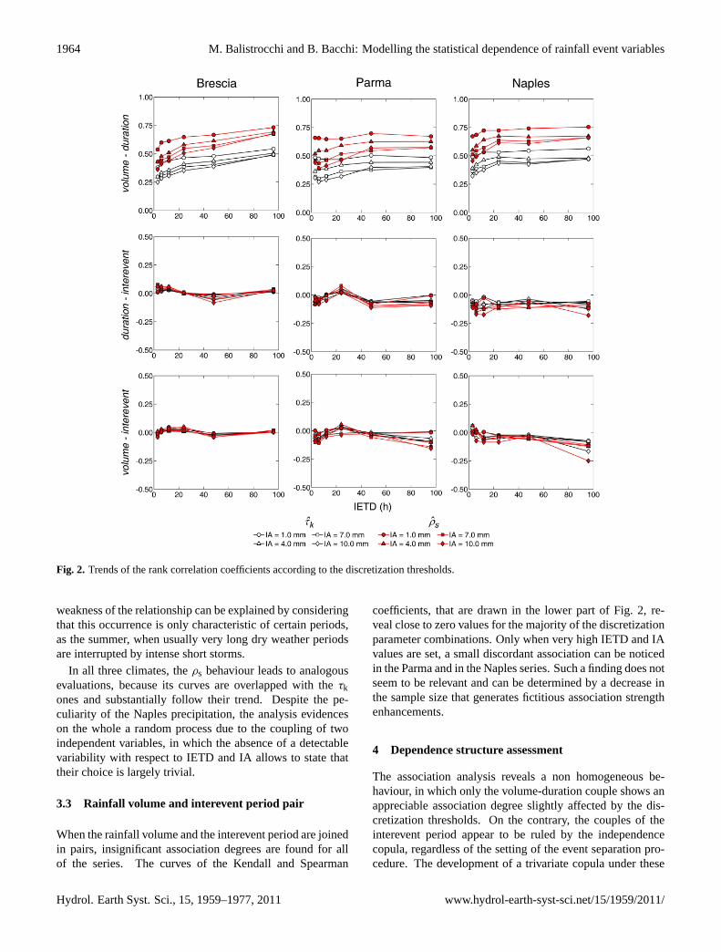
When the rainfall volume and the wet weather duration arecoupled, the Kendall measure exhibits substantially similartrends in the three locations, as the graphs in the upper partof Fig. 2 demonstrate. The coefficient always assumes posi-tive values from 0.25 to 0.55, outlining a moderately strongconcordance between the two variables. Although this rangeis relatively narrow, they tend to slightly increase with theminimum interevent time but to decrease with the volumethreshold. In fact, the weaker association occurs when the

minimum IETD and the maximum IA are set, while thegreater one corresponds to the opposite situation.

The first behaviour can be understood by considering theaggregation effect of an increasing IETD on the hyetographs:the longer the minimum interevent time, the greater the wetweather durations and the rainfall depths which characterizethe isolated storms are. In addition, the number of indepen-dent events decreases. As a result, the pseudo-observationvariability is diminished leading to a more concordant set ofpairs. Such a trend is more evident for the lower IETDs, be-cause of the many storm pulses separated by small intereventperiods which are present in the series. Further increases inits values determine minor effects and the curves practicallytend to assume a constant value.

The second one can only be explained by recognizing thatthe suppressed low depth events are mainly featured by shortdurations. Hence, those having high depths but short dura-tions, which form discordant pairs when they are coupledwith the major storms, remain in the sample and weaken theoverall dependence strength.

The correlation analysis performed by way of the Spear-man concordance measure, whose trends are drawn in thesame graphs of Fig. 2, delineates analogous outcomes. Thecurves of theρs coefficient are shifted upward with respectto the Kendall ones and the values are enclosed in the in-terval 0.35 and 0.65. Thus, in every climate the pseudo-observations seem to outline very similar dependence struc-tures that are quite different from those due to a couple ofindependent variables.

These results match the well known empirical evidence,since they confirm the existence of a non negligible statisticalassociation relating the total volume and the duration of anindividual storm, according to which the larger precipitationvolumes are tendentially generated by the longer wet weatherdurations. Moreover, its strength demonstrates to be largelyindependent of the raingauge location. Therefore, the precip-itation regime does not seem to represent a constituent factorin the assessment of this kind of dependence structure, unlikethe discretization parameters whose selection determines anappreciable variation in the rank correlation estimate.

3.2 Wet weather duration and interevent period pair

The Kendall and Spearman coefficients estimated for thecouple given by the wet weather duration and the intereventperiod yielded the identification of a negligible association inevery analysed climate. The plots in the middle part of Fig. 2evidence that the coefficient curves of the Brescia and theParma time series oscillate around the null value in the verysmall interval of−0.10 and 0.10. The Naples data are insteadcharacterized by a negative association, which however doesnot exceed the value of−0.15 for the largest IETD. Sucha discordant association agrees with the known behaviourof the mediterranean climate, in which short wet weatherdurations are separated by extended interevent times. The



Fig. 2. Trends of the rank correlation coefficients according to the discretization thresholds.

weakness of the relationship can be explained by consideringthat this occurrence is only characteristic of certain periods,as the summer, when usually very long dry weather periodsare interrupted by intense short storms.

In all three climates, theρs behaviour leads to analogousevaluations, because its curves are overlapped with theτkones and substantially follow their trend. Despite the pe-culiarity of the Naples precipitation, the analysis evidenceson the whole a random process due to the coupling of twoindependent variables, in which the absence of a detectablevariability with respect to IETD and IA allows to state thattheir choice is largely trivial.

3.3 Rainfall volume and interevent period pair

When the rainfall volume and the interevent period are joinedin pairs, insignificant association degrees are found for allof the series. The curves of the Kendall and Spearman

coefficients, that are drawn in the lower part of Fig. 2, re-veal close to zero values for the majority of the discretizationparameter combinations. Only when very high IETD and IAvalues are set, a small discordant association can be noticedin the Parma and in the Naples series. Such a finding does notseem to be relevant and can be determined by a decrease inthe sample size that generates fictitious association strengthenhancements.

4 Dependence structure assessment

The association analysis reveals a non homogeneous be-haviour, in which only the volume-duration couple shows anappreciable association degree slightly affected by the dis-cretization thresholds. On the contrary, the couples of theinterevent period appear to be ruled by the independencecopula, regardless of the setting of the event separation pro-cedure. The development of a trivariate copula under these



conditions therefore requires the use of a function able to suitthis very asymmetric dependence structure.

One of the most helpful advantages of the copula approachis actually the availability of a number of parametric copulafamilies, whose members can be defined in any multivari-ate case. The majority of models that have found practicalapplication is however fully defined by only one parameter,which is univocally determined by the association degree. Inour situation the overall concordance is expected to be lowwhen the three random variables are joined together. Thus,a one-parameter trivariate copula would be close to the in-dependence one and the observed concordance between theevent volume and the wet weather duration would not be cor-rectly modelled. Besides, in a multivariate framework hav-ing a dimension greater than two, the concordance estimateis controversial because its definition is ambiguous and com-plex (Salvadori et al., 2007).

A more convenient way is again given by the pairwiseanalysis, that can exploit various methods for constructingcopulas of higher dimension by mixing together also differ-ent bivariate functions; examples are given in Grimaldi andSerinaldi (2006) and Salvadori and De Michele (2006). Thistechnique appeared to be particularly appealing in this appli-cation and was utilized in the following development: firstlyone-parameter bivariate copulas were selected and fitted forthe three random vectors{xi , yi}, {yi , zi} and{xi , zi}, suc-cessively statistical tests were performed for assessing thegoodness-of-fit and finally the trivariate function was con-structed and further tested.

4.1 Copula function fitting

The selection of the most suitable copulas relies on the em-pirical copulasCn, whose general expression is written asfollows (Ruymgaart, 1973)

Cn(u) =1

n

n∑i=1

1(u1,i ≤ u1; ...; up,i ≤ up

); (7)

where u = (u1, ..., up) is a p-dimension random vectorbelonging to Ip, ui = (u1,i, ..., up,i) denotes a pseudo-observation vector,1(.) is the indicator function andn is thesample dimension.

This function computes the frequency of the pseudo-observations whose components do not exceed those of theu vector and approximates to the underlying copula, in thesame manner in which the sample frequency distributiontends to the marginal cumulative probability function. Be-ing Cn a consistent estimator (Deheuvels, 1979), it repre-sents the most objective tool for assessing the dependencestructure and can be efficaciously exploited for dealing withthe inference problem.

Herein, the copulas taken into consideration were thosebelonging to the one-parameter families of the Archimedeanclass, which includes absolutely continuous functions (awide discussion of their properties is provided by Nelsen,

2006, 106–156 pp.). The choice is justified by the advan-tages of their closed-form expressions and of their versatility,by which they are able to represent a variety of dependencestructures both in terms of form and strength. For these rea-sons, the Archimedean copulas have already found applica-tion in many hydrologic problems.

In this situation, the inference problem is simplified in theestimation of the dependence parameter, denoted byθ , of theunknown copulaC under the null hypothesis

H0 :C ∈ C0; (8)

by which the function is a member of a certain parametricfamily:

C0 = {Cθ : θ ∈ S} with S ⊆ R; (9)

beingS a subset of the real number setR.The fitting methods can be distinguished as either para-

metric or semiparametric, in consideration of whether the hy-potheses concerning the marginal distributions are involvedor not. The full likelihood criterion and the inference func-tion for margins (Joe, 1997) are parametric methods that em-ploy the Sklar theorem for developing a maximum likelihoodestimator where both the marginal and the copula parametersare included.

In the former, all the parameters are simultaneously es-timated by maximizing the log-likelihood function. In thelatter, the procedure is divided in two steps: firstly, only themarginal parameters are estimated, by using traditional con-sistent methods. Secondly, the fitted margins are introducedinto the log-likelihood function which is maximized to obtainthe copula ones. The inference function for margins requiresa smaller computational burden than the full likelihood crite-rion, but usually determines an efficiency loss of the estima-tor. Moreover, neither of them leaves the dependence param-eter estimation apart from the detriment due to wrong marginassumptions. In this case, the methods have been proved tobe affected by a severe bias (Kim et al., 2007).

One of the most popular semiparametric methods is basedon the pseudo-likelihood estimator, that may be expressed as:

L(θ) =

n∑i=1

log[cθ

(ui

)], (10)

wherecθ indicates the copula density (Genest et al., 1995;Shih and Louis, 1995). TheL(θ) function accounts exclu-sively for the pseudo-observation samples, which substitutethe marginal cdfs in the estimator argument.

Thus,L(θ) can be interpreted as a further development ofthe Joe inference function of margins, in which the marginalprobabilities are non-parametrically estimated. In generalthis estimator is less computationally intensive than the pre-vious ones but is not efficient, except for some particularcases (Genest and Werker, 2002).

When the dependence parameter is a scalar quantity, therelationships between the copula function and the concor-dance measure can be exploited to fit the copula with the



data by the method of moments. In fact, both the theo-retical versions of Kendallτk and Spearmanρs can be ex-pressed in terms of theθ parameter. The fitting procedurehence becomes very simple and consists in inverting suchrelationships and substituting the concordance measure esti-mates gathered from the pseudo-observations.

In our view, despite their limits, the semiparametric meth-ods represent more appropriate tools than the parametricones, because they are consistent with the copula approachaim, which consists in maintaining the dependence struc-ture assessment independent of those regarding the marginaldistributions. Either of these methods can be applied inour case, thanks to the absolute continuity properties of theArchimedean models, that always ensure the existence of thecopula density, and thanks to the need for estimating onlyone dependence parameter.

Considering the volume-duration pair, the most popularArchimedean copulas were fitted to the various random vec-tors{xi , yi} obtained by varying the IETD and the IA thresh-olds and they were visually compared to the correspondingempirical copulas. In the bivariate framework, this may becarried out by drawing the level curves of the two copu-las providing a rough, but effective, evaluation of the globalgoodness-of-fit.

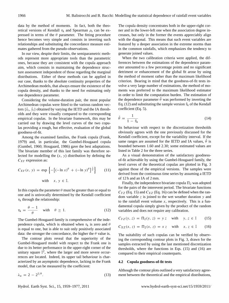
Among the examined families, the Frank copula (Frank,1979) and, in particular, the Gumbel-Hougaard copula(Gumbel, 1960; Hougaard, 1986) gave the best adaptations.The bivariate member of this last family was therefore se-lected for modelling the (x, y) distribution by defining theCXY expression as:

CXY (x, y) = exp{−

[(−ln x)θ + (−ln y)θ

] 1θ

}(11)

with x, y ∈ I.

In this copula the parameterθ must be greater than or equal toone and is univocally determined by the Kendall coefficientτk through the relationship:

τk =θ − 1

θwith θ ≥ 1. (12)

The Gumbel-Hougaard family is comprehensive of the inde-pendence copula, which is obtained whenτk is zero andθis equal to one, but is able to suit only positively associateddata: the stronger the concordance, the higher theθ value is.

The contour plots reveal that the superiority of theGumbel-Hougaard model with respect to the Frank one isdue to its better performance in the upper-right corner of theunitary squareI2, where the larger and more severe occur-rences are located. Indeed, its upper tail behaviour is char-acterized by an asymptotic dependence, lacking in the Frankmodel, that can be measured by the coefficient:

λu = 2 − 21/θ . (13)

The copula density concentrates both in the upper-right cor-ner and in the lower-left one when the association degree in-creases, but only in the former the events appreciably alignwith the diagonal. This means that such event variables arefeatured by a deeper association in the extreme storms thanin the common rainfalls, which emphasizes the tendency togenerate joined values.

When the two calibration criteria were applied, the dif-ferences between the estimations of the dependence param-eter amounted to a few percentage points and no significantdetriment or enhancement of the global fit arose by usingthe method of moment rather than the maximum likelihoodcriterion. Bearing in mind that the goodness-of-fit tests in-volve a very large number of estimations, the method of mo-ments was preferred to the maximum likelihood estimatorin order to limit the computation burden. The estimation ofthe dependence parameterθ was performed by inverting theEq. (12) and substituting the sample versionτk of the Kendallcoefficient (Eq. 5).

θ =1

1 − τk(14)

Its behaviour with respect to the discretization thresholdsobviously agrees with the one previously discussed for theKendall coefficient, except for the variability interval. If thesame ranges are assumed for the IETD and IA values,θ isbounded between 1.60 and 2.30; some estimated values arelisted in Table 2 for the three series.

As a visual demonstration of the satisfactory goodness-of-fit achievable by using the Gumbel-Hougaard family, thelevel curves of the theoretical copulas are plotted in Fig. 3against those of the empirical versions. The samples werederived from the continuous time series by assuming a IETDof 12 h and an IA of 2 mm.

Finally, the independence bivariate copula52 was adoptedfor the pairs of the interevent period. The bivariate functionsCYZ (Eq. 15) andCXZ (Eq. 16) can be defined when the ran-dom variablez is joined to the wet weather durationy andto the rainfall event volumex, respectively. This is a fun-damental copula simply given by the product of the randomvariables and does not require any calibration.

CYZ (y, z) = 52(y, z) = y z with y, z ∈ I (15)

CXZ (x, z) = 52(x, z) = x z with x, z ∈ I (16)

The suitability of such copulas can be verified by observ-ing the corresponding contour plots in Fig. 3, drawn for thesamples extracted by using the last mentioned discretizationthresholds, where the functions in Eqs. (15) and (16) arecompared to their empirical counterparts.

4.2 Copula goodness-of-fit tests

Although the contour plots outlined a very satisfactory agree-ment between the theoretical and the empirical distributions,



Table 2. Estimations of the dependence parameterθ for the precipitation series of Brescia, Parma [.], and Naples (.).

IETD IA (mm)

(h) 1 4 7 10

3 1.61 [1.94] (1.97) 1.42 [1.57] (1.64) 1.42 [1.46] (1.57) 1.33 [1.44] (1.48)6 1.75 [1.90] (2.02) 1.50 [1.62] (1.73) 1.45 [1.43] (1.63) 1.39 [1.37] (1.54)12 1.78 [1.88] (2.14) 1.55 [1.63] (1.86) 1.49 [1.47] (1.68) 1.44 [1.41] (1.60)24 1.87 [1.88] (2.13) 1.69 [1.72] (1.96) 1.62 [1.56] (1.83) 1.54 [1.47] (1.77)48 1.92 [2.02] (2.20) 1.77 [1.79] (1.90) 1.68 [1.60] (1.78) 1.63 [1.66] (1.74)96 2.19 [1.94] (2.29) 2.02 [1.80] (1.93) 1.95 [1.66] (1.89) 1.97 [1.68] (1.90)

Fig. 3. Contour lines of fitted copula functions and empirical copulas for samples extracted by using IETD = 12 h and IA = 4 mm.

a quantitative estimation of the goodness-of-fit by test statis-tic was found to be needed to ensure the model reliability.The test is formally stated with regard to the null hypothesisH0 (Eq. 8), under which the copulas were fitted. The ob-jective is to verify whether the underlying unknown copula

belongs to the chosen parametric family or such an assump-tion has to be rejected.

Several procedures have already been developed to meetthis task, as observed by Genest et al. (2009) who provided abrief review of the most popular ones. The various methods



are classified by the Authors in three main categories (i) thosethat can be utilized only for a specific copula family (Shih,1998; Malevergne and Sornette, 2003), (ii) those that have ageneral applicability but involve important subjective choicesfor their implementation, such as a parameter (Wang andWells, 2000), a smoothing factor (Scaillet, 2007) or a datacategorization (Junker and May, 2005), (iii) those that do nothave any of the previous constraints and for this reason arecalled blanket tests. The convenience of adopting the lastkind of test is clear and was highlighted by the Authors them-selves.

Furthermore, in the same paper, they analyzed the perfor-mances of some blanket procedures by way of large scaleMontecarlo simulations, obtaining a general confirmation oftheir validity. One of the most powerful tests is based on theempirical copula processCn defined as:

Cn =√n

(Cn − C

θ

), (17)

which evaluates the distance between the empirical copulaCn and the estimateC

θof the underlying copulaC under the

null hypothesisH0.A suitable test statisticSn can be constructed by using a

rank-based version of the Cramer-Von Mises criterion, aswritten in the integral:

Sn =

∫[0,1]p

Cn(u)2 dCn(u) with u ∈ Ip, (18)

whose integration variableu is a generic uniform randomvector havingp dimension. When theSn values are low,the fitted model and the pseudo-observation distribution areclose, on the contrary, they disagree considerably. In the firstcondition the null hypothesisH0 cannot be rejected, while inthe other it can.

Dealing with the pseudo-observationsui , the statisticSnmay be approximated by the sum:

Sn =

n∑i=1

[Cn

(ui

)− C

θ

(ui

)]2. (19)

As previously argued by Fermanian (2005) and successivelydemonstrated by Genest and Remilland (2008), the statis-tic Sn is able to yield an approximatep-value if it is im-plemented inside an appropriate parametric bootstrap proce-dure. According to the achievements previously discussed,in our case the procedure was implemented as follows, foreach of the three pairs of random variables:

– For a given combination of the parameter IETD and IA,n bivariate vectors of pseudo-observations are derivedby using the discretization procedure described in chap-ter 2, beingn the total number of independent storms.

– The sample Kendall coefficientτk and the empiricalcopulaCn are computed with respect to the observeddata by their expressions in Eqs. (5) and (7).

– The dependence parameterθ is estimated by the methodof moments, assessing the underlying copulaC

θ.

– The Cramer-Von Mises statisticSn is directly calculatedby Eq. (19), in which the analytical formulation of theArchimedean models is utilized.

– For a large integerN , the next sub-steps are repeated foreverym= 1, ...,N :

– A sample of pseudo-observations ofn dimension isgenerated by simulating the estimation of the un-derlying copulaC

θ.

– The sample Kendall coefficientτk,m and the empiri-cal copulaCn,m of the simulated data are computedby using their expressions in Eqs. (5) and (7).

– The dependence parameterθm is estimated by themethod of moments, assessing the theoretical cop-ulaC

θm.

– The Cramer-Von Mises statisticSn,m of the simu-lated sample is calculated by the same expressionof Eq. (19), in whichCn,m andC

θmare substituted

toCn andCθ, respectively.

– An approximatep-value is finally provided by the sum:

1

N

N∑m=1

1(Sn,m > Sn

). (20)

The tests were conducted varying the discretization parame-ters within the same IETD and IA ranges previously used forthe association measure analysis. Firstly, the real existenceof an association degree was verified by assuming that all thethree bivariate distributions correspond to the independent 2-copula (Eq. 21). When this assumption is tested, the proce-dure simplifies, because the steps concerning the estimationof the dependence parameter do not apply.

H0 :C = 52 (21)

Thep-values listed in Tables 3, 4 and 5 were obtained forthe three couples by assumingN greater than 2500. On thewhole, the independence assumption must be rejected for theevent volume and the wet weather duration pair, because nullor close to zerop-values are assessed, while for the other twovariable joints it cannot be rejected with significance levelsconsiderably greater than the usual values of the 5:10 %. Inaddition, no particular trends with regard to the IETD and IAsettings or differences among the climates are detected.

Hence, only for the first couple the null hypothesis (Eq.22), by which the dependence structure can be modeled bythe Gumbel-Hougaard 2-copula, was examined. Additionalgoodness-of-fit tests supplied the estimations that are listedin Table 6.

H0 :CXY ∈

{exp

{−


] 1θ

}: θ ∈ [1, ∞[

}(22)



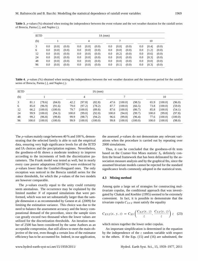
Table 3.p-values (%) obtained when testing the independence between the event volume and the wet weather duration for the rainfall seriesof Brescia, Parma [.], and Naples (.).

IETD IA (mm)

(h) 1 4 7 10

3 0.0 [0.0] (0.0) 0.0 [0.0] (0.0) 0.0 [0.0] (0.0) 0.0 [0.4] (0.0)6 0.0 [0.0] (0.0) 0.0 [0.0] (0.0) 0.0 [0.0] (0.0) 0.0 [1.2] (0.0)12 0.0 [0.0] (0.0) 0.0 [0.0] (0.0) 0.0 [0.2] (0.0) 0.0 [0.6] (0.0)24 0.0 [0.0] (0.0) 0.0 [0.0] (0.0) 0.0 [0.0] (0.0) 0.0 [0.3] (0.0)48 0.0 [0.0] (0.0) 0.0 [0.0] (0.0) 0.0 [0.0] (0.0) 0.0 [0.0] (0.0)96 0.0 [0.0] (0.0) 0.0 [0.0] (0.0) 0.0 [0.1] (0.0) 0.0 [0.3] (0.0)

Table 4. p-values (%) obtained when testing the independence between the wet weather duration and the interevent period for the rainfallseries of Brescia, Parma [.], and Naples (.).

IETD IA (mm)

(h) 1 4 7 10

3 81.1 [78.6] (84.0) 42.2 [97.8] (82.8) 47.6 [100.0] (98.5) 65.9 [100.0] (96.0)6 85.0 [96.9] (91.6) 79.0 [97.2] (78.2) 87.7 [100.0] (66.5) 73.8 [100.0] (59.0)12 66.2 [100.0] (100.0) 79.7 [100.0] (89.8) 87.6 [100.0] (86.7) 85.8 [100.0] (54.1)24 99.9 [100.0] (94.3) 100.0 [99.0] (92.0) 100.0 [94.0] (99.7) 100.0 [99.8] (97.8)48 99.2 [96.8] (99.8) 99.9 [98.7] (94.2) 96.6 [99.8] (96.4) 77.6 [100.0] (100.0)96 100.0 [100.0] (100.0) 99.9 [100.0] (100.0) 99.8 [100.0] (100.0) 100.0 [100.0] (98.0)

Thep-values mainly range between 40 % and 100 %, demon-strating that the selected family is able to suit the empiricaldata, ensuring very high significance levels for all the IETDand IA choices and the precipitation regimes. Nevertheless,the goodness-of-fit shows a moderate tendency to improveaccording to the increments of both the discretization pa-rameters. The Frank model was tested as well, but in nearlyevery case poorer adaptations (50:60 %) were evidenced byp-values lower than the Gumbel-Hougaard ones. The onlyexception was noticed in the Brescia rainfall series for theminor thresholds, for which thep-values of the two modelsare however comparable.

The p-values exactly equal to the unity could certaintyseem anomalous. The occurrence may be explained by thelimited numberN of repeated simulations that were per-formed, which was not set substantially larger than the sam-ple dimensionn as recommended by Genest et al. (2009) forlimiting the estimation variance. This choice was due to theneed to balance the assessment accuracy and the heavy com-putational demand of the procedure, since the sample sizescan greatly exceed two thousand when the lower values areutilized for the discretization thresholds. An iteration num-ber of 2500 has been considered by the same Authors as anacceptable compromise, that still allows to meet the main ob-jective of the test, even though a certain loss of the estimatorefficiency has to be accounted for. Indeed, in our application,

the assessedp-values do not demonstrate any relevant vari-ations when the procedure is carried out by repeating over2000 simulations.

Thus, it can be concluded that the goodness-of-fit testsbased on the Cramer-Von Mises statisticSn definitely con-firm the broad framework that has been delineated by the as-sociation measure analysis and by the graphical fits, since theassumed bivariate models cannot be rejected for the standardsignificance levels commonly adopted in the statistical tests.

4.3 Mixing method

Among quite a large set of strategies for constructing mul-tivariate copulas, the conditional approach that was investi-gated by Chakak and Koehler (1995) seemed to be extremelyconvenient. In fact, it is possible to demonstrate that thetrivariate copulaCXYZ must satisfy the equality

CXYZ (x, y, z) = CXY

(CXZ (x, z)

z,CYZ (y, z)

z

)z (23)

which mixes together the lower order copulas.

An important simplification is determined in the equationby the independence of thez random variable with respectto the others. If the Eqs. (15) and (16) are substituted, the



Table 5.p-values (%) obtained when testing the independence between the event volume and the interevent dry period for the rainfall seriesof Brescia, Parma [.], and Naples (.).

IETD IA (mm)

(h) 1 4 7 10

3 91.0 [100.0] (100.0) 100.0 [92.8] (94.2) 100.0 [90.4] (84.3) 99.8 [100.0] (100.0)6 98.0 [100.0] (100.0) 99.8 [88.8] (100.0) 100.0 [89.7] (99.5) 100.0 [99.8] (99.8)12 75.2 [100.0] (99.9) 100.0 [100.0] (99.3) 100.0 [99.8] (99.7) 98.4 [100.0] (99.4)24 94.8 [99.6] (100.0) 99.9 [99.6] (100.0) 99.5 [99.8] (100.0) 91.0 [100.0] (99.7)48 100.0 [100.0] (100.0) 100.0 [100.0] (100.0) 100.0 [100.0] (100.0) 100.0 [100.0] (100.0)96 100.0 [100.0] (99.4) 100.0 [99.4] (97.4) 100.0 [98.1] (99.8) 100.0 [99.5] (74.7)

Table 6. p-values (%) obtained when testing the goodness-of-fit of the Gumbel-Hougaard model to the event volume and the wet weatherduration pair for the rainfall series of Brescia, Parma [.], and Naples (.).

IETD IA (mm)

(h) 1 4 7 10

3 39.1 [100.0] (98.7) 77.2 [100.0] (99.8) 90.9 [99.9] (100.0) 100.0 [100.0] (99.8)6 77.0 [99.7] (99.2) 97.6 [100.0] (100.0) 100.0 [100.0] (99.6) 99.9 [100.0] (98.8)12 91.9 [100.0] (100.0) 96.8 [100.0] (100.0) 100.0 [100.0] (99.5) 99.9 [100.0] (99.2)24 99.7 [100.0] (100.0) 99.9 [100.0] (100.0) 100.0 [100.0] (100.0) 100.0 [100.0] (100.0)48 98.4 [100.0] (100.0) 100.0 [100.0] (100.0) 100.0 [100.0] (100.0) 100.0 [100.0] (100.0)96 100.0 [100.0] (100.0) 99.0 [100.0] (100.0) 91.7 [100.0] (100.0) 98.3 [100.0] (100.0)

equation of the trivariate copula is easily reduced to the prod-uct of the bivariate copulaCXY and the uniform variablez.

CXYZ (x, y, z) = CXY

(52(x, z)

z,52(y, z)

z

)z (24)

= CXY

(x z

z,y z

z

)z = CXY (x, y) z

Thus, the joint distribution suiting the natural variability ofthe individual rainfall event variables may be expressed bythe trivariate copula in Eq. (25), whose unique parameterθ

is exclusively a function of the positive association betweenthe event volume and the wet weather duration.

CXYZ (x, y, z) = exp

{−


] 1θ

}z (25)

When goodness-of-fit tests were performed for this trivariatecopula function,p-values mainly ranging between 40 % and100 % were found. Such a result was expected in view ofthe highp-values obtained in the pair analysis and definitelysupports the reliability of the proposed copula function forthe three precipitation regimes. The detailedp-value varia-tion with respect to the discretization thresholds is reportedin Table 7.

5 Marginal distribution assessment

Several probability models have been suggested for describ-ing the natural variability of the rainfall event characteristics,including the Gamma (Di Toro and Small, 1979; Wood andHebson, 1986), the Pareto (Salvadori and De Michele, 2006)and the Poisson functions (Wanielista and Yousef, 1992).Nonetheless, the most popular one is certainly the exponen-tial model, that has been extensively employed in a hugenumber of problems (a detailed list is provided in Salvadoriand De Michele, 2007). The reason for such a success mainlylies in its very simple formula, that often allows to analyti-cally integrate the derived probability functions and thereforemakes it particularly appealing in the analytical-probabilisticperspective.

Unfortunately, in the Italian precipitation regimes the ex-ponential model does not suit the observed distributions ofthe rainfall event variables. An appropriate alternative hasbeen identified in the Weibull model, that can be viewed as amore versatile generalization of the exponential one. Hence,the theoretical marginalsPV , PT andPA defined in Eq. (1)have been represented by means of the three cdfs in Eqs. (26),(27) and (28), respectively.

PV (v) =

1 − exp

[−

(v − IAζ

)β]for v ≥ IA

0 otherwise(26)



Table 7.p-values (%) obtained when testing the trivariate copula for the rainfall series of Brescia, Parma [.], and Naples (.).

IETD IA (mm)

(h) 1 4 7 10

3 43.3 [98.7] (99.7) 41.3 [99.8] (95.2) 73.0 [99.8] (94.4) 99.5 [99.9] (99.5)6 75.0 [99.9] (99.7) 70.4 [98.2] (98.2) 96.6 [99.9] (95.8) 80.0 [99.5] (91.9)12 65.0 [100.1] (92.1) 87.6 [100.0] (98.2) 93.1 [100.0] (99.6) 83.0 [99.7] (82.6)24 99.0 [99.5] (99.9) 99.8 [96.6] (99.9) 99.4 [79.1] (100.0) 96.8 [99.3] (99.8)48 97.7 [99.9] (100.1) 99.9 [100.0] (99.4) 99.4 [100.0] (98.5) 98.6 [100.0] (99.9)96 100.0 [100.0] (96.9) 99.4 [100.0] (99.5) 91.8 [98.0] (99.9) 99.2 [99.2] (67.5)

PT (t) =

{1 − exp

[−

(tλ

)γ ]for t ≥ 0

0 otherwise(27)

PA(a) =

1 − exp

[−

(a − IETD

ψ

)δ]for a ≥ IETD

0 otherwise(28)

The exponentsβ, γ andδ are dimensionless parameters thatrule the shape of the distributions, while the denominatorsζ

(mm),λ (h) andψ (h) define the scale of the random process.The IA and the IETD parameters represent the lower limitsin Eqs. (26) and (28) and are set in accordance with the min-imum interevent time and the volume threshold employed inthe rainfall separation procedure.

In this kind of model the correct assessment of the expo-nent is a key aspect, because very dissimilar shapes of theprobability density function (pdf) are possible with respect toits value: (i) when an exponent smaller than one occurs, thepdf monotonically decreases from the lower limit in which avertical asymptote is present, (ii) when it is exactly equal toone, the pdf owns a finite mode in the lower limit but doesnot lose the monotonic decreasing behaviour, (iii) when it ex-ceeds the unity the distribution mode is greater than the lowerlimit and the pdf exhibits a right tail that is progressively lessmarked if it is further incremented. Hence, the greater the ex-ponent, the more shifted to the right the most probable valuesare and the more symmetric the distribution is.

5.1 Marginal function fitting

A sensitivity analysis has been carried out referring to thepreviously investigated IETD and IA ranges. The marginaldistributions were fitted to the sample data extracted from thecontinuous rainfall series by the maximum likelihood crite-rion yielding the graphs plotted in Fig. 4 for the shape pa-rameters and in Fig. 5 for the scale ones: on the whole, it canbe argued that the precipitation regime does not significantlyaffect the estimation of the margin parameters, since almostidentical behaviours are evidenced.

The shape parametersβ and δ are always less than theunity, because they lie within the intervals 0.60:0.98 and0.55:0.90, respectively; on the contrary, the exponentγ of

the storm duration cdf may be greater than one, being es-timated between 0.80:1.35. As mentioned above, the unityrepresents a fundamental boundary for the shape parameter.Therefore, unlike the other two distributions, the duration pdfmay be subject to important changes in shape with referenceto the discretization parameter settings.

For all the three exponents, greater values are generally es-timated when the volume threshold increases, while differenttrends are evidenced with respect to the minimum intereventtime. In fact, theδ exponent increases with the IETD, but theopposite behaviour occurs for theγ exponent and, finally,no clear tendency can be detected for theβ exponent. Thescale parametersζ , λ andψ are instead characterized by awider variability, by which they increase according to boththe discretization thresholds in quite a proportional manner.

The reasons for such outcomes reside in the effects of thediscretization thresholds, illustrated in the association anal-ysis context. The scale parameters mainly depend on themean, whose increments can be immediately justified by theisolation of more extended events separated by longer dryweather periods. The shape parameters are instead essen-tially related to the variance; given the wide scale variability,the dispersion around the mean must be discussed by usingthe coefficient of variation, which is exclusively a function ofthe exponent.

The properties of the Weibull probability function are suchthat the exponent increase is related to a reduction of the co-efficient of variation. In fact, if the volume threshold is incre-mented the frequency of the smallest observations decreasesfor all three variables, diminishing the overall distributiondispersion. An analogous explanation may be advanced forunderstanding the effects of the IETD extension on the drywhether period distribution, because the minimum intereventtime directly acts on the variable as a threshold.

This filtering action is not systematically exercised on thewet weather durations, whose minor values do not alwaysdisappear from the sample. In fact, when the rainfalls are iso-lated by long interevent periods, as in the dry seasons, theyare not aggregated in more extended events. The mean in-crease therefore occurs along with a larger enhancement of



Fig. 4. Trends of the margin shape parameters according to the discretization thresholds.

the standard deviation, leading to the reduction of the coeffi-cient of variation.

Finally, the lack of a recognizable trend of the rainfallvolume dispersion with respect to the IETD appears to bereasonable because this discretization parameter operates re-gardless of this quantity: even storms having completely dif-ferent depths may be joined into a unique event and so thedispersion change is not univocally foreseeable.

The scale parameters deserve a last consideration because,albeit they do not seem to be sensitive to the precipitationregime, they evidence however to be influenced by anotherclimatic aspect such as the annual precipitation amount. Ob-viously, in the wetter climates, greaterζ andλ values havebeen estimated, while the dryer ones were found to be fea-tured by largerψ . A demonstration of this assertion canbe found in Fig. 5 by observing the curves belonging to theParma series, whose annual mean depth is the lowest amongthe presented cases.

5.2 Marginal goodness-of-fit tests

The suitability of the Weibull probabilistic model for repre-senting the natural variability of the rainfall event volumeshas already been proved by using the confidence boundarytest for the Brescia time series (Bacchi et al., 2008). In thiswork, the same technique has been adopted for assessing thegoodness-of-fit in all the illustrated Italian climates regardingthe complete set of random variables. The tests are intendedto verify whether the Weibull distributions from Eq. (26) toEq. (28), fitted by way of the maximum likelihood method,can be rejected or not according to an a priori fixed signif-icance level. They are based on the standard variablesυ, τandα defined for the event volume, the wet weather durationand the interevent periods respectively

υ =v − IA

ζ; τ =

t

λ; α =

a − IETD

ψ, (29)



Fig. 5. Trends of the margin scale parameters according to the discretization thresholds.

The corresponding sample versions are easily obtained byinverting the cdfs and substituting the frequenciesF (Eq. 2)to the non exceedance probabilityP :

υ =

[ln

(1

1 − FV

)] 1β

; τ =

[ln

(1

1 − FT

)] 1γ

; (30)

α =

[ln

(1

1 − FA

)] 1δ

.

The confidence limits were centered with respect to the the-oretical value and quantified for a significance level of 5 %by using the interval half-width1 in Eq. (31), computed as afunction of the non exceedance probabilityP and the proba-bility densityp of the standard variable.

1 = ±1.96√n

√P (1 − P)

p(31)

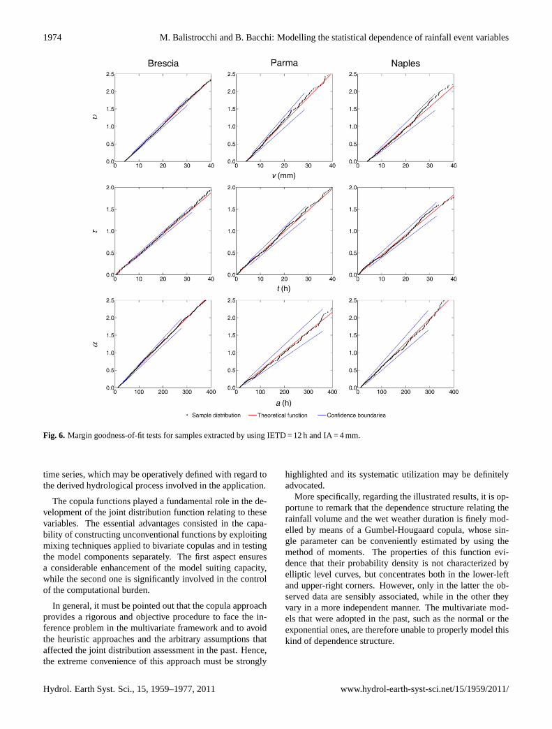
An example of the goodness-of-fit achievable by means ofthe Weibull probabilistic model is illustrated in the plots of

Fig. 6, in which the confidence boundaries are drawn be-tween the probability interval 0.20:0.80 and the sample dataare derived from the continuous record by using the thresh-olds IETD = 12 h and IA = 4 mm. The sample points arefairly aligned with the theoretical line and substantially en-compassed in the confidence region. Analogous results weregathered from all the series by using different sets of IETDand IA. Thus, in general, the hypothesis concerning the as-sumed probabilistic function cannot be rejected.

6 Conclusions

In this work the possibility of analysing the stochastic struc-ture of the rainfall point process by a quite simple trivariatejoint distribution has been clearly demonstrated. Such a dis-tribution is based on three random variables able to representthe storm main features, the rainfall volume, the wet weatherduration and the interevent period. The sample constructionneeds a criterion for isolating independent events from the



Fig. 6. Margin goodness-of-fit tests for samples extracted by using IETD = 12 h and IA = 4 mm.

time series, which may be operatively defined with regard tothe derived hydrological process involved in the application.

The copula functions played a fundamental role in the de-velopment of the joint distribution function relating to thesevariables. The essential advantages consisted in the capa-bility of constructing unconventional functions by exploitingmixing techniques applied to bivariate copulas and in testingthe model components separately. The first aspect ensuresa considerable enhancement of the model suiting capacity,while the second one is significantly involved in the controlof the computational burden.

In general, it must be pointed out that the copula approachprovides a rigorous and objective procedure to face the in-ference problem in the multivariate framework and to avoidthe heuristic approaches and the arbitrary assumptions thataffected the joint distribution assessment in the past. Hence,the extreme convenience of this approach must be strongly

highlighted and its systematic utilization may be definitelyadvocated.

More specifically, regarding the illustrated results, it is op-portune to remark that the dependence structure relating therainfall volume and the wet weather duration is finely mod-elled by means of a Gumbel-Hougaard copula, whose sin-gle parameter can be conveniently estimated by using themethod of moments. The properties of this function evi-dence that their probability density is not characterized byelliptic level curves, but concentrates both in the lower-leftand upper-right corners. However, only in the latter the ob-served data are sensibly associated, while in the other theyvary in a more independent manner. The multivariate mod-els that were adopted in the past, such as the normal or theexponential ones, are therefore unable to properly model thiskind of dependence structure.



This provides a reason for the difficulties encountered inthe stochastic representation of the dependent hydrologicalvariables. On the contrary, when the interevent dry periodis joined to the other variables, the independence hypothe-sis cannot be rejected, confirming the reliability of the tradi-tional assumption.

The ability of the three parameter Weibull function to fitthe marginal distributions of all the analysed random vari-ables was also statistically tested. In the proposed formula-tion, the distribution lower limit is a priori fixed with refer-ence to the independent event discretization procedure, whilethe other two may be estimated by the maximum likelihoodcriterion. The main appeal of using this alternative model liesin its analytical form, that neither compromises the modelversatility required by the sample data nor complicates theparameter assessment.

The analysis took into consideration three time series,which are representative of as many Italian rainfall regimes.Despite the variability of their meteorological characteris-tics, the analysis revealed that, when the thresholds employedfor isolating the independent storms change, both the depen-dence structure and the margins show identical behaviours.Moreover, very similar fitting values were estimated for theirparameters, except for those expressing the univariate dis-tribution scale which demonstrated to be moderately influ-enced by the total annual rainfall depth. A very satisfactoryagreement between theoretical functions and observed datais outlined by the performed statistical tests, for every coupleof IETD and IA values that were considered. Thus, a gen-eral reliability of the proposed probabilistic model may bededuced for the Italian climates.

The natural research development could be addressed tothe flood frequency analysis, by exploiting deterministic orstochastic routing models, or to the watershed hydrologicbalance, considered both in its global terms and in its com-ponents, infiltration and evapotranspiration. Even though theproposed model has quite a simple expression, its implemen-tation in the derivation procedure should reasonably yieldpdfs that cannot be analytically integrated. The model ef-fectiveness advance will have to be carefully appraised inconsideration of such an inconvenience, since the capabil-ity of the analytical-probabilistic methodology to express thederived probability functions by an analytical expression rep-resents one of the most important advantages that justifies itsuse.

Finally, another research perspective is offered by the con-cerns involved in the estimation of the return period. In fact,in the multivariate case its evaluation still remains an openquestion, because a universally accepted definition has notbeen proposed yet. The main reason lies in the ambiguityof having very different events associated with the same fre-quency of occurrence, which arises from the most immediategeneralizations of this concept. The analytical-probabilisticmethodology offers a way of facing this problem from the

univariate point of view, because the forcing meteorologicalvariables are directly related to the dependent one.

Acknowledgements.Giuseppe De Martino of the UniversityFederico II and his research group are kindly acknowledged forhaving provided the Naples precipitation data. The reviewersand Gianfausto Salvadori of the University of Lecce are alsoacknowledged for their useful suggestions and fruitful discussions.The research was supported by grants from the University ofBrescia.

Edited by: A. Montanari

References

Adams, B. J., and Papa, F.: Urban stormwater management plan-ning with analytical probabilistic models, John Wiley & Sons,New York, 2000.

Bacchi, B., Becciu, G., and Kottegoda, N. T.: Bivariate exponentialmodel applied to intensities and durations of extreme rainfall, J.Hydrol., 155(1–2), 225–236,doi:10.1016/0022-1694(94)90166-X, 1994.

Bacchi, B., Balistrocchi, M., and Grossi, G.: Proposal of a semi-probabilistic approach for storage facility design, Urban WaterJ., 5(3), 195–208,doi:10.1080/15730620801980723, 2008.

Balistrocchi, M., Grossi, G., and Bacchi, B.: An analytical prob-abilistic model of the quality efficiency of a sewer tank, WaterResour. Res., 45, W12420,doi:10.1029/2009WR007822, 2009.

Bandini, A.: Tipi pluviometrici dominanti sulle regioni italiane,Servizio Idrografico Italiano, Roma, Italy, 1931.

Beven, K. J.: Rainfall-runoff modelling: the primer, John Wi-ley & Sons, Bath, UK, 2001.

Bonta, J. V. and Rao, A. R.: Factors affecting the identifica-tion of independent storm events, J. Hydrol., 98(3–4), 275–293,doi:10.1016/0022-1694(88)90018-2, 1988.

Chakak, A. and Koehler, K. J.: A strategy for constructing multi-variate distributions, Commun. Stat. Simulat., 24(3), 537–550,doi:10.1080/03610919508813257, 1995.

Chan, S.-O. and Bras, R. L.: Urban storm water management: dis-tribution of flood volumes, Water Resour. Res., 15(2), 371–382,doi:10.1029/WR015i002p00371, 1979.

Chow, V. T., Maidment, D. R., and Mays, L. W.: Applied hydrology,McGraw-Hill International Edition, New York, NY, USA, 1988.

Cordova, J. R. and Rodrıguez-Iturbe, I.: On the probabilistic struc-ture of storm surface runoff, Water Resour. Res., 21(5), 755–763,doi:10.1029/WR021i005p00755, 1985.

Cox, D. R. and Isham, V.: Point processes, Chapman and Hall Ltd.,London, UK, 1980.

Deheuvels, P.: Empirical dependence function and properties: non-parametric test of independence, Bulletin de la classe des sci-ences Academie Royale de Belgique, 65(6), 274–292, 1979.

Di Toro, D. M. and Small, M. J.: Stormwater interception and stor-age, J. Environ. Eng.-ASCE, 105(1), 43–54, 1979.

Dıaz-Granados, M. A., Valdes, J. B., and Bras, R. L.: A physicallybased flood frequency distribution, Water Resour. Res., 20(7),995–1002,doi:10.1029/WR020i007p00995, 1984.

Eagleson, S. P.: Dynamic hydrology, McGraw-Hill, New York,USA, 1970.


http://dx.doi.org/10.1016/0022-1694(94)90166-X

http://dx.doi.org/10.1016/0022-1694(94)90166-X

http://dx.doi.org/10.1080/15730620801980723

http://dx.doi.org/10.1029/2009WR007822

http://dx.doi.org/10.1016/0022-1694(88)90018-2

http://dx.doi.org/10.1080/03610919508813257

http://dx.doi.org/10.1029/WR015i002p00371




Eagleson, S. P.: Dynamics of flood frequency, Water Resour. Res.,8(4), 878–898,doi:10.1029/WR008i004p00878, 1972.

Eagleson, S. P.: Climate, soil, and vegetation 2. The dis-tribution of annual precipitation derived from observedstorm sequences, Water Resour. Res., 14(5), 713–721,doi:10.1029/WR014i005p00713, 1978a.

Eagleson, S. P.: Climate, soil, and vegetation 5. A derived distribu-tion of storm surface runoff, Water Resour. Res., 14(5), 741–748,doi:10.1029/WR014i005p00741, 1978b.

Eagleson, S. P.: Climate, soil and vegetation 7. A derived distribu-tion of annual water yield, Water Resour. Res., 14(5), 765–776,doi:10.1029/WR014i005p00765, 1978c.

Fermanian, J.-D.: Goodness-of-fit tests for copulas, J. Multivar.Anal., 95(1), 119–152,doi:10.1016/j.jmva.2004.07.004, 2005.

Foufoula-Georgiou, E. and Guttorp, P.: Assessment of a class ofNeyman-Scott models for temporal rainfall, J. Geophys. Res.,92(D8), 9679–9682,doi:10.1029/JD092iD08p09679, 1987.

Frank, M. J.: On the simultaneous associativity ofF(x,y)and x + y − F(x,y), Aequationes Math., 19(1), 194–226,doi:10.1007/BF02189866, 1979.

Genest, C. and Remilland, B.: Validity of the parametric bootstrapfor goodness-of-fit testing in semiparametric models, Annalesde l’Institut Henri Poincare: Probabilites et Statistiques, 44 (6),1096–1127, 2008.

Genest, C. and Werker, B. J. M.: Conditions for the asymptoticsemiparametric efficiency of an omnibus estimator of depen-dence parameters in copula models, in: Distribution with GivenMarginals and Statistical Modelling, Kluwer, Dordrecht, TheNederlands, 103–112, 2002.

Genest, C., Ghoudi, K., and Rivest, L.-P.: A semiparamet-ric estimation procedure of dependence parameters in multi-variate families of distributions, Biometrika, 82(3), 543–552,doi:10.1093/biomet/82.3.543, 1995.

Genest, C., Remilland, B., and Beaudoin, D.: Goodness-of-fit testsfor copulas: a review and a power study, Insur. Math. Econ.,44(2), 199–213,doi:10.1016/j.insmatheco.2007.10.005, 2009.

Goel, N. K., Kurothe, R. S., Mathur, B. S., and Vogel, R. M.: A de-rived flood frequency distribution for correlated rainfall intensityand duration, J. Hydrol., 228(1–2), 56–67,doi:10.1016/S0022-1694(00)00145-1, 2000.

Grimaldi, S. and Serinaldi, F.: Asymmetric copula in multivariateflood frequency analysis, Adv. Water Resour., 29(8), 1115–1167,doi:10.1016/j.advwatres.2005.09.005, 2006.

Gumbel, E. J.: Distributions des valeurs extremes en plusieurs di-mensions, Publ. Inst. Statist. Univ. Paris 9, 171–173, 1960.

Guo, Y. and Adams, B. J.: Hydrologic analysis of urbancatchments with event-based probabilistic models 2. Peakdischarge rate, Water Resour. Res., 34(12), 3433–3443,doi:10.1029/98WR02448, 1998.

Guo, Y. and Adams, B. J.: An analytical probabilistic approachto sizing flood control detention facilities, Water Resour. Res.,35(8), 2457–2468,doi:10.1029/1999WR900125, 1999.

Hougaard, P.: A class of multivariate failure time distributions,Biometrika, 73(3), 671–678,doi:10.1093/biomet/73.3.671,1986.

Joe, H.: Multivariate models and dependence concepts, Chapmanand Hall, London, 1997.

Junker, M. and May, A.: Measurement of aggregate risk withcopulas, Economet. J., 8(3), 428–454,doi:10.1111/j.1368-423X.2005.00173.x, 2005.

Kendall, M. G.: A new measure of the rank correlation, Biometrika,30(1–2), 81–93,doi:10.1093/biomet/30.1-2.81, 1938.

Kim, G., Silvapulle, M. J., and Silvapulle, P.: Compari-son of semiparametric and parametric methods for estimat-ing copulas, Comput. Stat. Data. An., 51(6), 2836–2850,doi:10.1016/j.csda.2006.10.009, 2007.

Kruskal, W. H.: Ordinal Measures of Association, J. Am. Stat. As-soc., 53(284), 814–861,doi:10.2307/2281954, 1958.

Kurothe, R. S., Goel, N. K., and Mathur, B. S.: Derivedflood frequency distribution for negatively correlated rainfall in-tensity and duration, Water Resour. Res., 33(9), 2103–2107,doi:10.1029/97WR00812, 1997.

Li, J. Y. and Adams, B. J.: Probabilistic models for analysis of ur-ban runoff control systems, J. Environ. Eng., 126(3), 217–224,doi:10.1061/(ASCE)0733-9372(2000)126:3(217), 2000.

Malevergne, Y. and Sornette, D.: Testing the Gaussian copula hy-pothesis for financial assets dependences, Quant. Financ., 3(4),231–250,doi:10.1088/1469-7688/3/4/301, 2003.

Moisello, U.: Grandezze e fenomeni idrologici, La GoliardicaPavese, 1985.

Nelsen, R. B.: An introduction to copulas, 2 edition, Springer, NewYork, 2006.

Restrepo-Posada, P. J. and Eagleson, P. S.: Identificationof independent rainstorms, J. Hydrol., 55(1–4), 303–319,doi:10.1016/0022-1694(82)90136-6, 1982.

Ruymgaart, F. H.: Asymptotic theory for rank tests for indepen-dence, MC Tract 43, Amsterdam, Mathematisch Instituut, 1973.

Salvadori, G. and De Michele, C.: Statistical characterization oftemporal structure of storms, Adv. Water Resour., 29(6), 827–842,doi:10.1016/j.advwatres.2005.07.013, 2006.

Salvadori, G. and De Michele, C.: On the use of copulas in hydrol-ogy: theory and practice, J. Hydrol. Eng.-ASCE, 12(4), 369–380,doi:10.1061/(ASCE)1084-0699(2007)12:4(369), 2007.

Salvadori, G., De Michele, C., Kottegoda, N. T., and Rosso, R.:Extremes in nature: an approach using copulas, Springer, Dor-drecht, The Nederlands, 2007.

Scaillet, O.: Kernel-based goodness-of-fit tests for copulas withfixed smoothing parameters, J. Multivar. Anal., 98(3), 533–543,doi:10.1016/j.jmva.2006.05.006, 2007.

Seto, M. Y. K.: Comparison of alternative derived probability distri-bution models for urban stormwater management, M.A.Sc. the-sis, Department of Civil Engineering, University of Toronto,Toronto, Ontario, 1984.

Shih, J. H.: A goodness-of-fit test for association in a bi-variate survival model, Biometrika, 85(1), 189–200,doi:10.1093/biomet/85.1.189, 1998.

Shih, J. H. and Louis, T. A.: Inferences on the association parameterin copula models for bivariate survival data, Biometrics, 51(4),1384–1399, 1995.

Singh, K. and Singh, V. P.: Derivation of bivariate probability den-sity functions with exponential marginals, Stoch. Hydrol. Hy-draul., 5(1), 55–68,doi:10.1007/BF01544178, 1991.

Sklar, A.: Fonctions de repartitiona n dimensions et leures marges,Publ. Inst. Statist. Univ. Paris 8, 229–231, 1959.






http://dx.doi.org/10.1016/j.jmva.2004.07.004

http://dx.doi.org/10.1029/JD092iD08p09679

http://dx.doi.org/10.1007/BF02189866

http://dx.doi.org/10.1093/biomet/82.3.543

http://dx.doi.org/10.1016/j.insmatheco.2007.10.005

http://dx.doi.org/10.1016/S0022-1694(00)00145-1

http://dx.doi.org/10.1016/S0022-1694(00)00145-1

http://dx.doi.org/10.1016/j.advwatres.2005.09.005

http://dx.doi.org/10.1029/98WR02448

http://dx.doi.org/10.1029/1999WR900125


http://dx.doi.org/10.1111/j.1368-423X.2005.00173.x

http://dx.doi.org/10.1111/j.1368-423X.2005.00173.x

http://dx.doi.org/10.1093/biomet/30.1-2.81

http://dx.doi.org/10.1016/j.csda.2006.10.009

http://dx.doi.org/10.2307/2281954

http://dx.doi.org/10.1029/97WR00812

http://dx.doi.org/10.1061/(ASCE)0733-9372(2000)126:3(217)

http://dx.doi.org/10.1088/1469-7688/3/4/301

http://dx.doi.org/10.1016/0022-1694(82)90136-6

http://dx.doi.org/10.1016/j.advwatres.2005.07.013

http://dx.doi.org/10.1061/(ASCE)1084-0699(2007)12:4(369)

http://dx.doi.org/10.1016/j.jmva.2006.05.006


http://dx.doi.org/10.1007/BF01544178


Stuart, A. and Ord, J. K.: Kendall’s advanced theory of statistics,5th edition, Vol. 2, Edward Arnold, London, UK, 1991.

Vandenberghe, S., Verhoest, N. E. C., and De Baets, B.: Fitting bi-variate copulas to the dependence structure between storm char-acteristics: a detailed analysis based on 105 year 10 min rainfall,Water Resour. Res., 46, W01512,doi:10.1029/2009WR007857,2010.

Wang, W. J. and Wells, M. T.: Model selection and semiparamet-ric inference for bivariate failure-time data, J. Am. Stat. Assoc.,95(449), 62–72, 2000.

Wanielista, M. P. and Yousef, Y. A.: Stormwater management, JohnWiley & Sons, New York, 1992.

Waymire, E., Gupta, V. K., and Rodriguez-Iturbe, I.: A spectral the-ory of rainfall intensity at the meso-β scale, Water Resour. Res.,20(10), 1453–1465,doi:10.1029/WR020i010p01453, 1984.

Wood, E. F. and Hebson, C. S.: On hydrologic similarity 1. Deriva-tion of the dimensionless flood frequency curve, Water Re-sour. Res., 22(11), 1549–1554,doi:10.1029/WR022i011p01549,1986.


http://dx.doi.org/10.1029/2009WR007857



Documents

Modelling the statistical dependence of rainfall event … · 2015-02-03 · storm random variables which are supposed to be indepen- ... The ﬁrst hydrological application of the