Models and Modelingin the High SchoolPhysics Classroom

Presentation Objectives

• The problem with conventional instruction• Key features of Modeling Instruction• The Modeling Cycle

• sample pre-lab activity• evaluation of data• post-lab extension - development of kinematic

equations• deployment exercises

The Problem with Traditional Instruction

• It presumes two kinds of knowledge: facts and knowhow.

• Facts and ideas are things that can be packaged into words and distributed to students.

• Knowhow can be packaged as rules or procedures.

• We come to understand the structure and behavior of real objects only by constructing models.

“Teaching by Telling” is Ineffective

• Students usually miss the point of what we tell them.

• Key words or concepts do not elicit the same “schema” for students as they do for us.

• Watching the teacher solve problems does not improve student problem-solving skills.

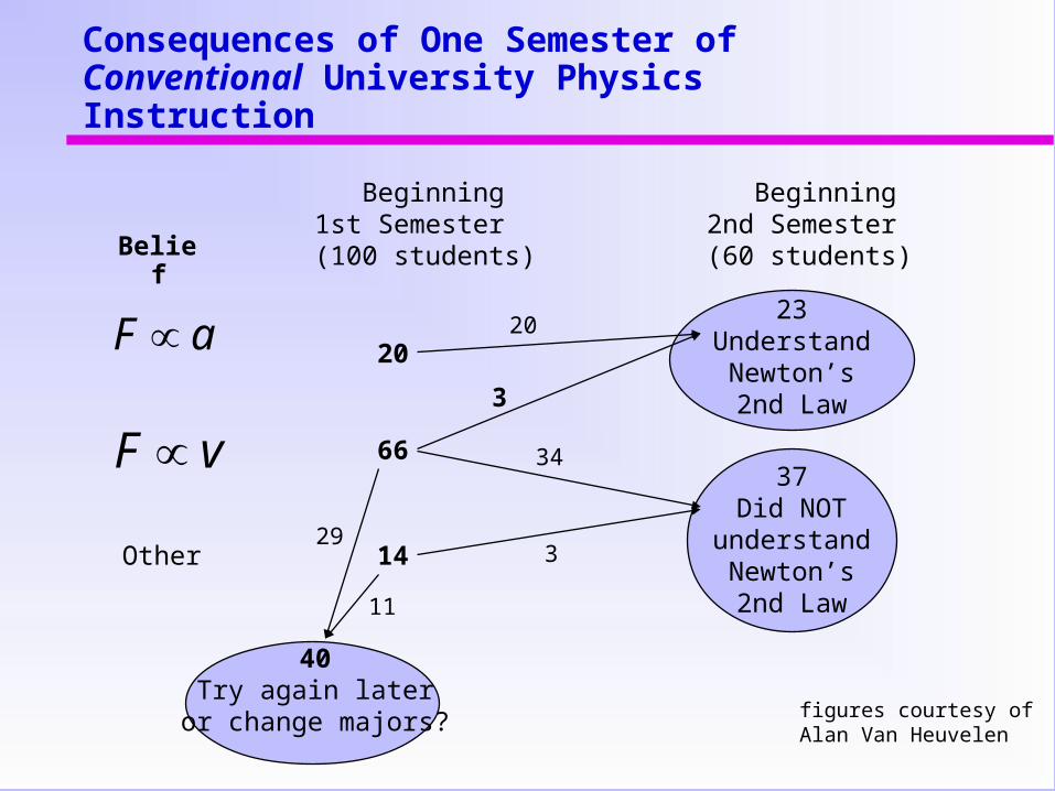
Consequences of One Semester of Conventional University Physics Instruction

figures courtesy ofAlan Van Heuvelen

Belief

Beginning1st Semester(100 students)

Beginning2nd Semester(60 students)

40Try again later

or change majors?

Other

20

66

14

23UnderstandNewton’s2nd Law

37Did NOT

understandNewton’s2nd Law

293

11

20

3

34

F ∝ a

F ∝ v

Instructional Objectives

• Construct and use scientific models to describe, to explain, to predict and to control physical phenomena.

• Model physical objects and processes using diagrammatic, graphical and algebraic representations.

• Small set of basic models as the content core of physics.

• Evaluate scientific models through comparison with empirical data.

• Modeling as the procedural core of scientific knowledge.

Why modeling?!• To make students’ classroom experience closer to

the scientific practice of physicists.• To make the coherence of scientific knowledge

more evident to students by making it more explicit.

• Construction and testing of math models is a central activity of research physicists.

• Models and Systems are explicitly recognized as major unifying ideas for all the sciences by the AAAS Project 2061 for the reform of US science education.

• Robert Karplus made systems and models central to the SCIS elementary school science curriculum.

Models vs Problems• The problem with problem-solving

• Students come to see problems and their answers as the units of knowledge.• Students fail to see common elements in novel problems.

» “But we never did a problem like this!”

• Models as basic units of knowledge• A few basic models are used again and again with only minor modifications.• Students identify or create a model and make inferences from the model to produce a solution.

What Do We Mean by Model?

• with explicit statements of the relationships between these representations

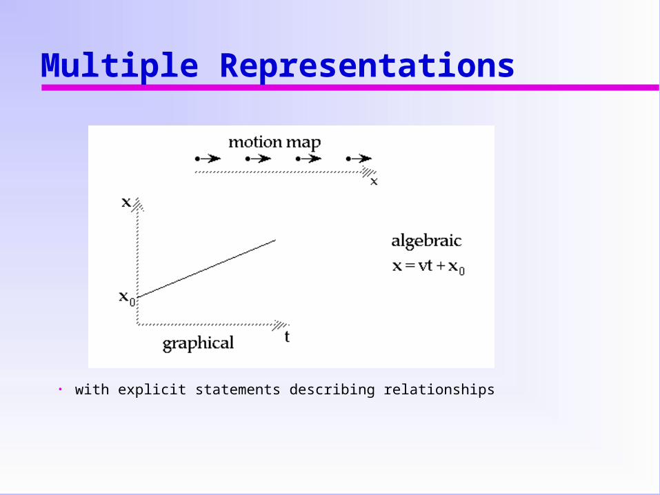
Multiple Representations

• with explicit statements describing relationships

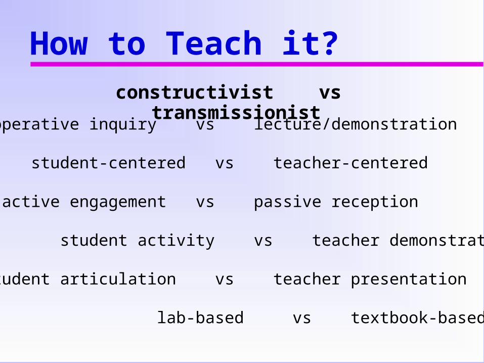
constructivist vs transmissionist

cooperative inquiry vs lecture/demonstration

student-centered vs teacher-centered

active engagement vs passive reception

student activity vs teacher demonstration

student articulation vs teacher presentation

lab-based vs textbook-based

How to Teach it?

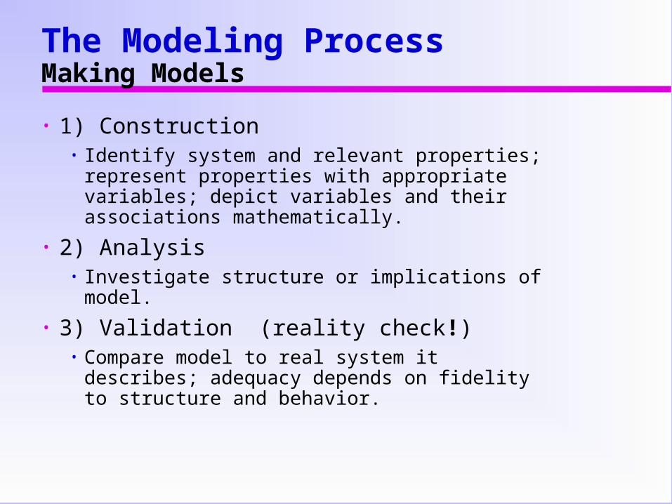
The Modeling ProcessMaking Models

• 1) Construction• Identify system and relevant properties;

represent properties with appropriate variables; depict variables and their associations mathematically.

• 2) Analysis• Investigate structure or implications of model.

• 3) Validation (reality check!)• Compare model to real system it describes;

adequacy depends on fidelity to structure and behavior.

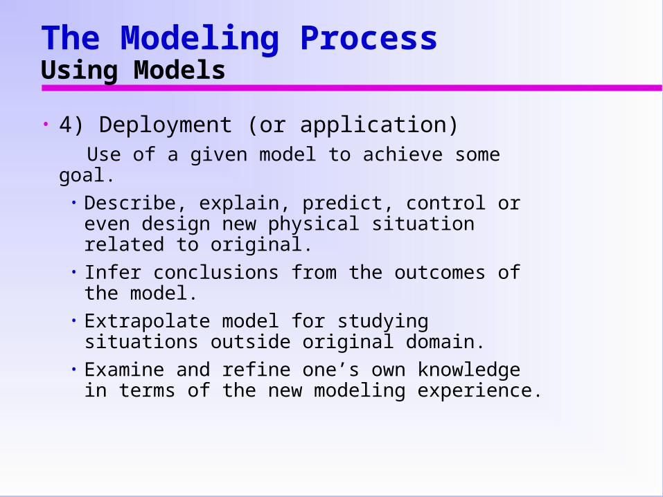
The Modeling ProcessUsing Models

• 4) Deployment (or application) Use of a given model to achieve some goal.

• Describe, explain, predict, control or even design new physical situation related to original.

• Infer conclusions from the outcomes of the model.

• Extrapolate model for studying situations outside original domain.

• Examine and refine one’s own knowledge in terms of the new modeling experience.

Modeling Cycle• Development begins with paradigm

experiment.• Experiment itself is not remarkable.• Instructor sets the context.• Instructor guides students to

• identify system of interest and relevant variables.

• discuss essential elements of experimental design.

I - Model Development• Students in cooperative groups

• design and perform experiments.• use computers to collect and analyze

data.• formulate functional relationship

between variables.• evaluate “fit” to data.

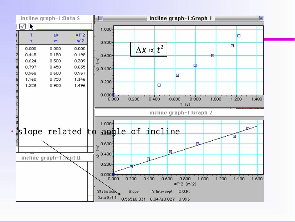
• slope related to angle of incline

Δx ∝ t2

I - Model Development

• Post-lab analysis

• whiteboard presentation of student findings

• multiple representations»verbal»diagrammatic»graphical»algebraic

• justification of conclusions

II - Model Deployment

• In post-lab extension, the instructor• brings closure to the experiment.• fleshes out details of the model, relating

common features of various representations.• helps students to abstract the model from the

context in which it was developed.

Post-Lab ExtensionRecall Constant Velocity Lab

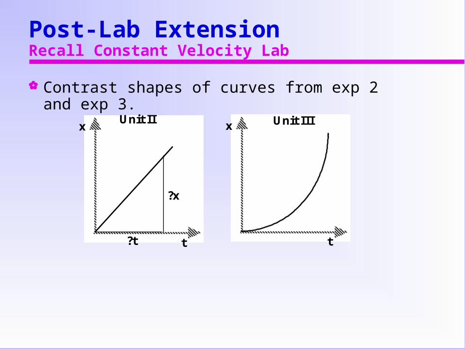
Contrast shapes of curves from exp 2 and exp 3.

x x

t t

?x

?t

Unit II Unit III

Post-Lab ExtensionInstantaneous velocity

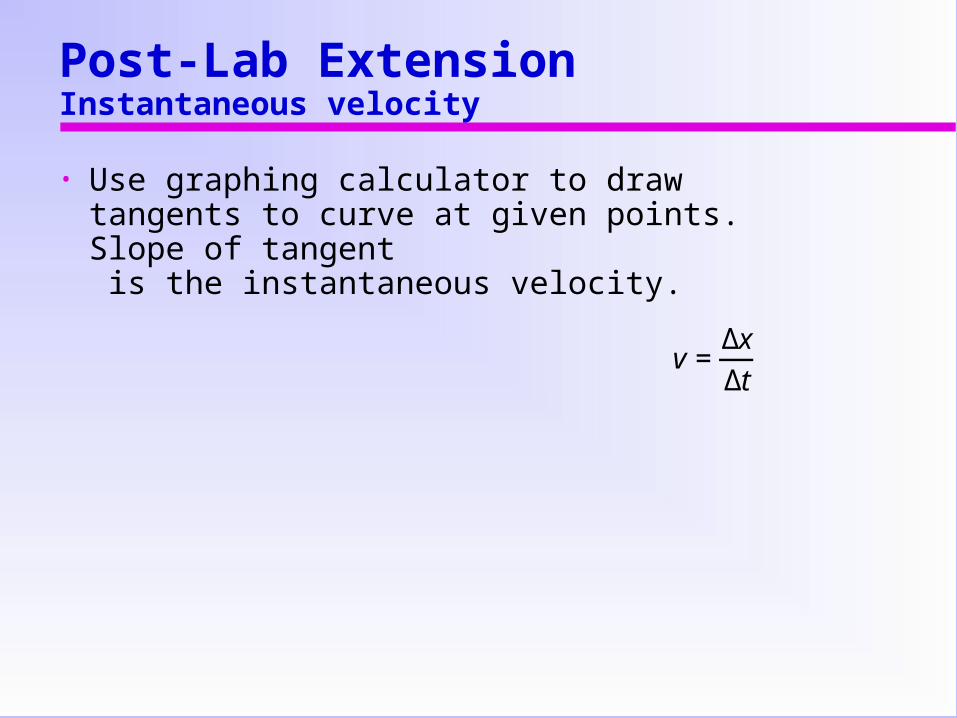
• Use graphing calculator to draw tangents to curve at given points. Slope of tangent is the instantaneous velocity.

v =ΔxΔt

Post-Lab ExtensionInstantaneous Velocity Exercise

v (m/ s)

t (s)

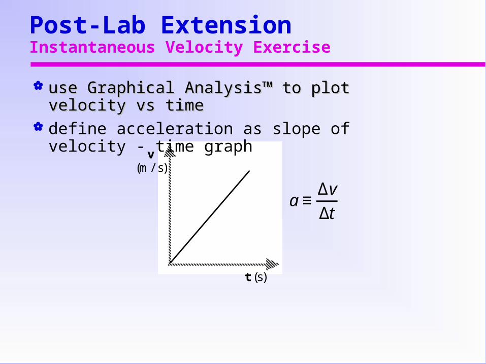
a≡ΔvΔt

use Graphical Analysis™ to plot velocity vs use Graphical Analysis™ to plot velocity vs timetime

define acceleration as slope of velocity - time graph

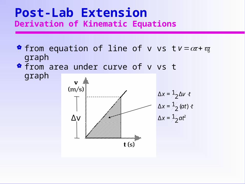
Post-Lab ExtensionDerivation of Kinematic Equations

from equation of line of v vs t graph v =at+v0

from area under curve of v vs t graph

∆v

Δx =12Δv⋅t

Δx =12(at) ⋅t

Δx =12at2

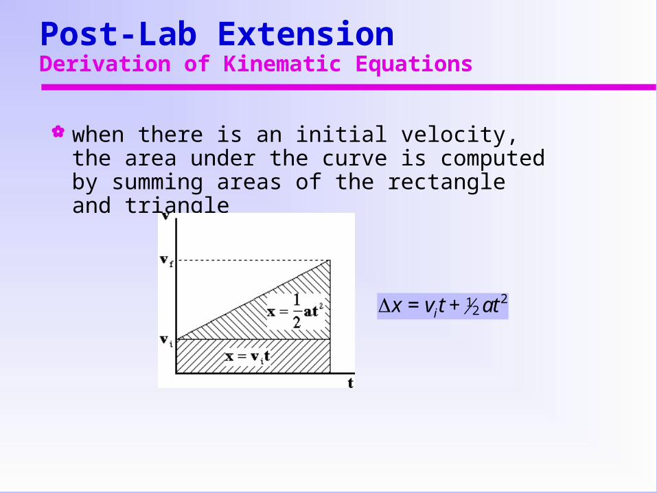
when there is an initial velocity, the area under the curve is computed by summing areas of the rectangle and triangle

Post-Lab ExtensionDerivation of Kinematic Equations

Δx = vit + 12 at

2

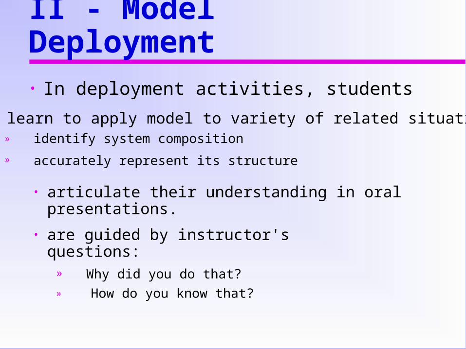
II - Model Deployment• In deployment activities, students

• articulate their understanding in oral presentations.

• are guided by instructor's questions:» Why did you do that?» How do you know that?

• learn to apply model to variety of related situations.» identify system composition

» accurately represent its structure

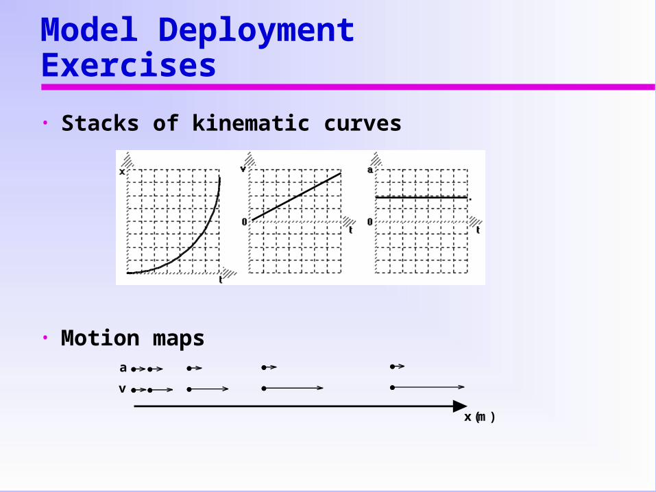
Model Deployment Exercises

• Stacks of kinematic curves

• Motion maps

x (m)

v

a

• Newtonian concepts developed• distinction between instantaneous and

average velocity• acceleration as rate of change in velocity

• Emphasis on physical interpretation of graphs

• slope of tangent to curve in x vs t graph• slope of v vs t graph• area under curve in a vs t graph

Descriptive Particle Models: Kinematics- Uniform Acceleration

Model Deployment ExercisesPatrolman and speeder

• Multiple solutions (algebraic, diagrammatic, graphical)

• Graphical Analysis™ to produce x vs t graph

Model Deployment ExercisesPatrolman and speeder

• Area under v vs t graph yields displacement.

• Objectives:• to improve the quality of scientific discourse.• move toward progressive deepening of student

understanding of models and modeling with each pass through the modeling cycle.

• get students to see models everywhere!

II - Model Deployment

• Ultimate Objective:• autonomous scientific thinkers fluent in all

aspects of conceptual and mathematical modeling.

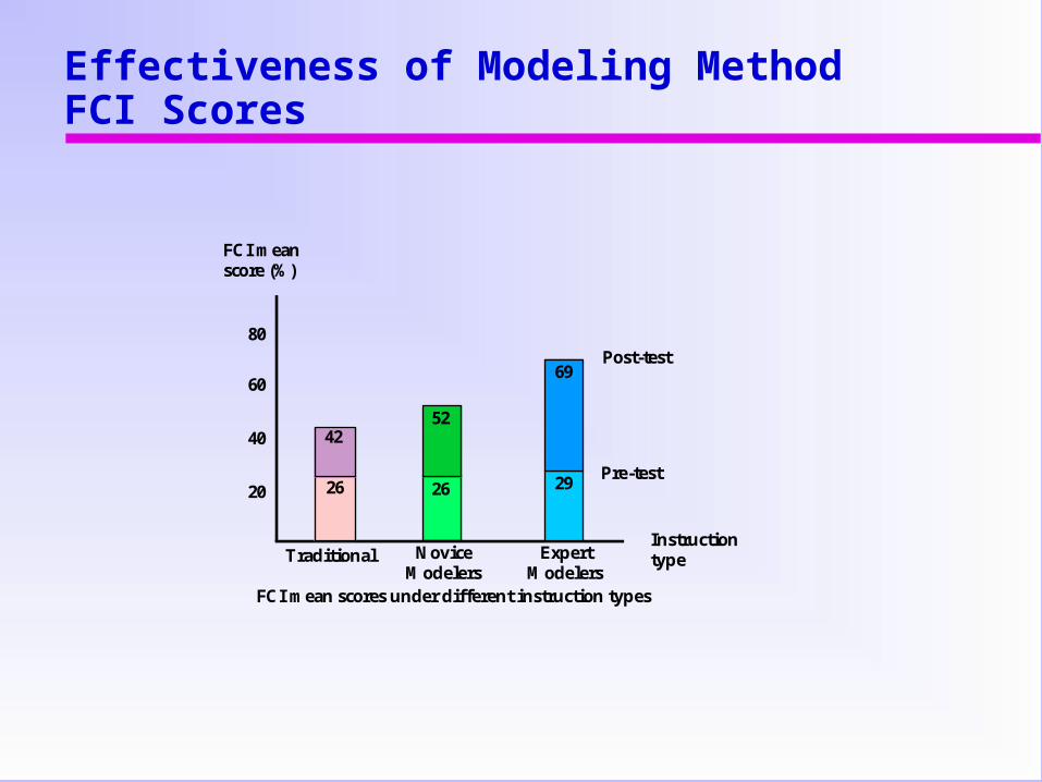
Effectiveness of Modeling MethodFCI Scores

20

40

60

80

26

4252

29

69

Traditional NoviceModelers

FCI meanscore (%)

Post-test

Pre-test

FCI mean scores under different instruction types

InstructiontypeExpert

Modelers

26

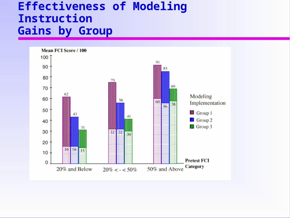
Effectiveness of Modeling InstructionGains by Group

Modeling Instruction Program

• Coordinates professional development opportunities nationwide

• for further information, contact Dr. Jane Jackson

Box 871504 Dept. of Physics & Astronomy Arizona State University Tempe, AZ 85287

voice (480) 965-8438 email: jane.jackson@asu.edu check out our home page http://modeling.asu.edu/