34

Models for Ordinal Outcomes（（（（有序多分有序多分有序多分有序多分类类类类变量变量变量变量模型模型模型模型）））） 3.1 Ordinal outcomes

− The categories of an ordinal variable can be ranked but the distances between the categories are unknown. For example, in survey research, opinions are often ranked as strongly agree, agree, disagree, and strongly disagree.

− Distributional Assumptions and Ordinal Regression Model (ORM) • ordered probit model )1,0(~ Nε （有序概率单元模型）

• ordered logit model )3,0(~ πλε （有序胜算对数模型） − Simply because the values of a variable can be ordered does not imply that the

variable should be analyzed as ordinal. − A variable can be ordered when being considered for one purpose, but be

unordered or ordered differently when being used for another purpose. For instance, occupational grouping can be ordered both by the status of the occupations and by the income of the occupations but can also be treated as non-ordered categories.

− Thus, if the proper ordering is ambiguous, models for nominal variables should be considered.

3.2 The Statistical Model

− The ORM can be developed in different ways, each of which leads to the same form of the model. These approaches to the model parallel those for the BRM. The BRM can be considered as a special case of the ORM, which the ordinal outcome has only two categories.

3.2.1 A Latent Variable Model（隐性变量模型）：assume a latent or unobserved variable y* ranging from -∞ to ∞ that is related to the observed independent variable by

− The measurement model for binary outcomes is expanded to divide y* into J ordinal categories

J to1mfor if *1 =<<= − mimi ymy ττ

− The link between the observed outcomes and the latent y* can be made with the following example:

• People are asked to respond to the statement: “A working mother can establish just as warm and secure of a relationship with her child as a mother

iii Xy εβ +=*

35

who does not work.” Reponses were coded as: 1=strongly disagree (SD), 2=disagree (D), 3=agree (A), and 4=strongly agree (SA).

• Define the observed variable as

∞=<≤⇒

<≤⇒

<≤⇒

<≤−∞=⇒

=

ifSA 4

ifA 3

if D 2

if SD1

4*

3

3*

2

2*

1

1*

0

ττττττ

ττ

i

i

i

i

i

y

y

y

y

y

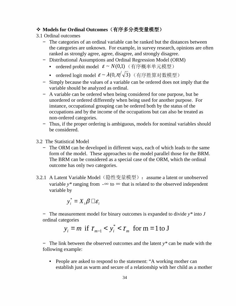
• Graphically:

The solid line represents the latent variable y*. The cutpoints are indicated by the horizontal lines marked τ1, τ2, and τ3. The values of the observed variable y over the range of y* are marked below with a dotted line.

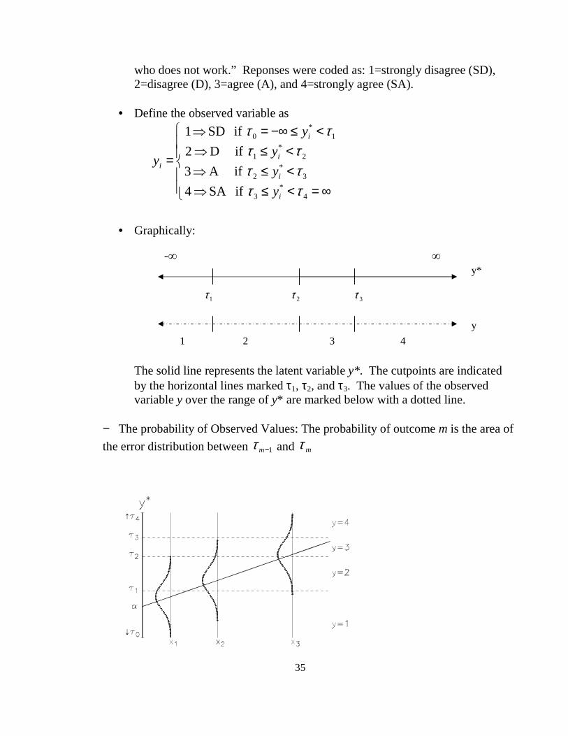
− The probability of Observed Values: The probability of outcome m is the area of

the error distribution between 1−mτ and mτ

-∞ ∞

2τ 1τ 3τ

1 2 3 4

y*

y

36

– the standard formula for the predicted probability in the ORM is

)()()|Pr( 1 βτβτ xFxFxmy mm −−−== − 3.2.2 A Nonlinear Probability Model（非线性概率模型）: The ORM can also be

derived without appealing to latent variable through specifying a nonlinear model relating the xs to the probability of an event • First, the odds that an outcome is less than or equal to m versus greater than

m given x is defined as

1-J 1,mfor )|Pr(

)|Pr()(| =

>≤≡Ω >≤ Xmy

XmyXmm

• The log of the odds is assumed to equal

βτ xx mmm −=Ω >≤ )(ln |

– Example: Mother’s relationship with her Child （职业妇女与亲子关系）(file name: ordwarm2 ). The model to be estimated is

prstageedwhitemaleyrx

xFxFxmwarm

prstageedwhitemaleyr

mmi

βββββββ

βτβτ

+++++=

−−−== −

89

where

)()()|Pr(

89

1

– Estimation with STATA (a do-file)

*including version number ensures compatibility wit h later Stata release version 11 * if a log file is open, close it capture log close *don’t pause when output scrolls off the page set more off *log results to file brm_binlfp2 log using orm_ordwarm2, replace *open data file ordwarm2 use ordwarm2, clear

37

*describe provides information of the dataset describe *summarize provides summary statistics summarize *output from ologit and oprobit and store the resul ts ologit warm yr89 male white age ed prst

(or statistics/ordinal outcomes/ordered logistic regression) estimates store ologit oprobit warm yr89 male white age ed prst estimate store oprobit *combining the results in a table estimates table ologit oprobit, b(%9.3f) se label v arwidth(30)

Output page *including version number ensures compatibility wit h later Stata release . version 11 . . * if a log file is open, close it . capture log close . *don't pause when output scrolls off the page . set more off . *log results to file orm_ordwarm2 . log using orm_ordwarm2, replace . *open data file ordwarm2 . use ordwarm2, clear (77 & 89 General Social Survey) . *describe provides information of the dataset . describe Contains data from ordwarm2.dta obs: 2,293 77 & 89 General Social Survey vars: 10 3 May 2001 09:54 size: 32,102 (99.7% of memory free) (_dta has notes) --------------------------------------------------- -------------------------- storage display value variable name type format label varia ble label --------------------------------------------------- -------------------------- warm byte %10.0g SD2SA Mom c an have warm relations w/ child yr89 byte %10.0g yrlbl Surve y year: 1=1989 0=1977 male byte %10.0g sexlbl Gende r: 1=male 0=female white byte %10.0g racelbl Race: 1=white 0=not white age byte %10.0g Age i n years ed byte %10.0g Years of education prst byte %10.0g Occup ational prestige warmlt2 byte %10.0g SD 1=SD; 0=D,A,SA

38

warmlt3 byte %10.0g SDD 1=SD, D; 0=A,SA warmlt4 byte %10.0g SDDA 1=SD, D,A; 0=SA --------------------------------------------------- -------------------------- Sorted by: warm . *summarize provides summary statistics . summarize Variable | Obs Mean Std. Dev. Min Max -------------+------------------------------------- ------------------- warm | 2293 2.607501 .9282156 1 4 yr89 | 2293 .3986044 .4897178 0 1 male | 2293 .4648932 .4988748 0 1 white | 2293 .8765809 .3289894 0 1 age | 2293 44.93546 16.77903 18 89 -------------+------------------------------------- ------------------- ed | 2293 12.21805 3.160827 0 20 prst | 2293 39.58526 14.49226 12 82 warmlt2 | 2293 .1295246 .3358529 0 1 warmlt3 | 2293 .4448321 .4970556 0 1 warmlt4 | 2293 .8181422 .3858114 0 1 . *output from ologit and oprobit and store the res ults . ologit warm yr89 male white age ed prst, nolog Ordered logit estimates N umber of obs = 2293 L R chi2(6) = 301.72 P rob > chi2 = 0.0000 Log likelihood = -2844.9123 P seudo R2 = 0.0504 --------------------------------------------------- --------------------------- warm | Coef. Std. Err. z P>| z| [95% Conf. Interval] -------------+------------------------------------- --------------------------- yr89 | .5239025 .0798988 6.56 0.0 00 .3673037 .6805013 male | -.7332997 .0784827 -9.34 0.0 00 -.8871229 -.5794766 white | -.3911595 .1183808 -3.30 0.0 01 -.6231815 -.1591374 age | -.0216655 .0024683 -8.78 0.0 00 -.0265032 -.0168278 ed | .0671728 .015975 4.20 0.0 00 .0358624 .0984831 prst | .0060727 .0032929 1.84 0.0 65 -.0003813 .0125267 -------------+------------------------------------- --------------------------- _cut1 | -2.465362 .2389126 (Anci llary parameters) _cut2 | -.630904 .2333155 _cut3 | 1.261854 .2340179 --------------------------------------------------- --------------------------- . estimates store ologit . oprobit warm yr89 male white age ed prst, nolog Ordered probit estimates N umber of obs = 2293 L R chi2(6) = 294.32 P rob > chi2 = 0.0000 Log likelihood = -2848.611 P seudo R2 = 0.0491

39

--------------------------------------------------- --------------------------- warm | Coef. Std. Err. z P>| z| [95% Conf. Interval] -------------+------------------------------------- --------------------------- yr89 | .3188147 .0468519 6.80 0.0 00 .2269867 .4106427 male | -.4170287 .0455459 -9.16 0.0 00 -.5062971 -.3277603 white | -.2265002 .0694773 -3.26 0.0 01 -.3626733 -.0903272 age | -.0122213 .0014427 -8.47 0.0 00 -.0150489 -.0093937 ed | .0387234 .0093241 4.15 0.0 00 .0204485 .0569982 prst | .003283 .001925 1.71 0.0 88 -.0004899 .0070559 -------------+------------------------------------- --------------------------- _cut1 | -1.428578 .1387742 (Anci llary parameters) _cut2 | -.3605589 .1369219 _cut3 | .7681637 .1370564 --------------------------------------------------- --------------------------- . estimates store oprobit . *combining the results in a table . estimates table ologit oprobit, b(%9.3f) se label varwidth(30) --------------------------------------------------- ----- Variable | ologit oprob it -------------------------------+------------------- ----- Survey year: 1=1989 0=1977 | 0.524 0. 319 | 0.080 0. 047 Gender: 1=male 0=female | -0.733 -0. 417 | 0.078 0. 046 Race: 1=white 0=not white | -0.391 -0. 227 | 0.118 0. 069 Age in years | -0.022 -0. 012 | 0.002 0. 001 Years of education | 0.067 0. 039 | 0.016 0. 009 Occupational prestige | 0.006 0. 003 | 0.003 0. 002 _cut1 | -2.465 -1. 429 | 0.239 0. 139 _cut2 | -0.631 -0. 361 | 0.233 0. 137 _cut3 | 1.262 0. 768 | 0.234 0. 137 --------------------------------------------------- ----- legend: b/se

As with the BRM, the estimated coefficients differ from logit to probit by a factor of about 1.7, reflecting the differing scaling of the ordered logit and order probit models.

Values of the z-tests are very similar because they are not affected by the scaling, but they are not identical because of slight differences in the shape of the assumed distribution of the errors.

3.3 Hypothesis Testing with test and lrtest

– If the assumptions of the model hold, the ML estimators from ologit and oprobit are distributed asymptotically normally and thus can be tested with the corresponding z-statistics in the output

40

– The z-test included in the output of estimation command is a Wald test, which can be computed using test . For example, to test 0:0 =maleH β ,

*significant test of a single coefficient quietly ologit warm yr89 male white age ed prst test male

Output page . quietly ologit warm yr89 male white age ed prst . test male ( 1) male = 0 chi2( 1) = 87.30 Prob > chi2 = 0.0000

We conclude that gender significant affects attitudes toward working mothers.

– test can be used to test multiple coefficients. For example, to test

0:0 === malewhiteageH βββ ,

*significant test of multiple coefficients test age white male

Output page . *significant test of multiple coefficients . test age white male ( 1) age = 0 ( 2) white = 0 ( 3) male = 0 chi2( 3) = 166.62 Prob > chi2 = 0.0000

The hypothesis that the demographic effects of age, race, and gender are simultaneously equal to zero can be rejected at the .01 level.

– Comparing competitive (nested) models using LR test:

*comparing nested models using an LR test ologit warm yr89 male white age ed prst, nolog estimates store fmodel

41

ologit warm yr89 ed prst, nolog estimates store nmodel lrtest fmodel nmodel

Output page . quietly ologit warm yr89 male white age ed prst, nolog . estimates store fmodel . quietly ologit warm yr89 ed prst, nolog . estimates store nmodel . lrtest fmodel nmodel likelihood-ratio test LR chi2(3) = 171.58 (Assumption: nmodel nested in fmodel) Prob > chi2 = 0.0000

The hypothesis that the demographic effects of age, race, and gender are simultaneously equal to zero can be rejected at the .01 level.

3.4 Interpretation: 3.4.1 Predicted Probabilities with predict

After fitting a model with ologit or oprobit , a useful first step is to compute the predicted probabilities with command prdict

* Predicted Probabilities with predict ologit warm yr89 male white age ed prst, nolog predict SDologit Dlogit Alogit SAlogit summarize SDologit Dlogit Alogit SAlogit dotplot SDologit Dlogit Alogit SAlogit

(or graphics/distributional graphs/distribution dotplot)

Output page . * Predicted Probabilities with predict . ologit warm yr89 male white age ed prst, nolog Ordered logit estimates N umber of obs = 2293 L R chi2(6) = 301.72 P rob > chi2 = 0.0000 Log likelihood = -2844.9123 P seudo R2 = 0.0504 --------------------------------------------------- --------------------------- warm | Coef. Std. Err. z P>| z| [95% Conf. Interval] -------------+------------------------------------- --------------------------- yr89 | .5239025 .0798988 6.56 0.0 00 .3673037 .6805013 male | -.7332997 .0784827 -9.34 0.0 00 -.8871229 -.5794766 white | -.3911595 .1183808 -3.30 0.0 01 -.6231815 -.1591374 age | -.0216655 .0024683 -8.78 0.0 00 -.0265032 -.0168278 ed | .0671728 .015975 4.20 0.0 00 .0358624 .0984831 prst | .0060727 .0032929 1.84 0.0 65 -.0003813 .0125267 -------------+------------------------------------- --------------------------- _cut1 | -2.465362 .2389126 (Anci llary parameters)

42

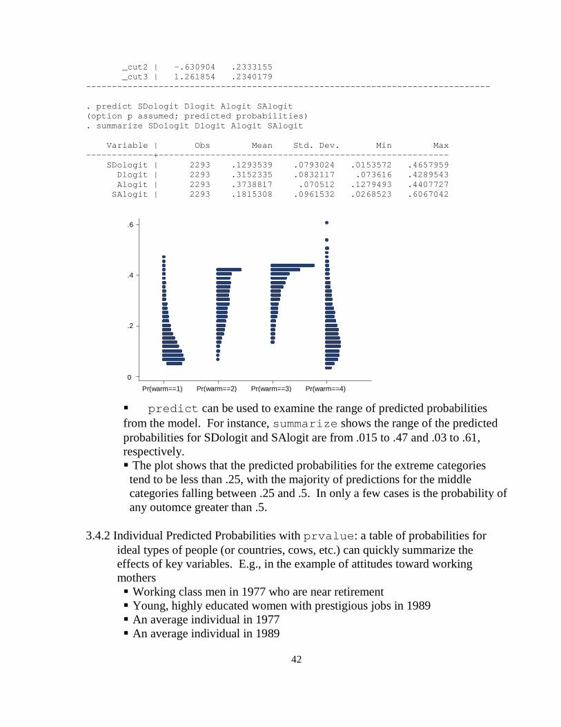
_cut2 | -.630904 .2333155 _cut3 | 1.261854 .2340179 --------------------------------------------------- --------------------------- . predict SDologit Dlogit Alogit SAlogit (option p assumed; predicted probabilities) . summarize SDologit Dlogit Alogit SAlogit Variable | Obs Mean Std. Dev. Min Max -------------+------------------------------------- ------------------- SDologit | 2293 .1293539 .0793024 .0153572 .4657959 Dlogit | 2293 .3152335 .0832117 .073616 .4289543 Alogit | 2293 .3738817 .070512 .1279493 .4407727 SAlogit | 2293 .1815308 .0961532 .0268523 .6067042

predict can be used to examine the range of predicted probabilities from the model. For instance, summarize shows the range of the predicted probabilities for SDologit and SAlogit are from .015 to .47 and .03 to .61, respectively. The plot shows that the predicted probabilities for the extreme categories tend to be less than .25, with the majority of predictions for the middle categories falling between .25 and .5. In only a few cases is the probability of any outomce greater than .5.

3.4.2 Individual Predicted Probabilities with prvalue : a table of probabilities for

ideal types of people (or countries, cows, etc.) can quickly summarize the effects of key variables. E.g., in the example of attitudes toward working mothers Working class men in 1977 who are near retirement Young, highly educated women with prestigious jobs in 1989 An average individual in 1977 An average individual in 1989

0

.2

.4

.6

Pr(warm==1) Pr(warm==2) Pr(warm==3) Pr(warm==4)

43

* using prvalue to compute ideal types ologit warm yr89 male white age ed prst, nolog prvalue, x(yr89=0 male=1 age=64 prst=20 ed=12) rest (mean) prvalue, x(yr89=1 male=0 prst=80 ed=24) rest(mean) prvalue, x(yr89=0) rest(mean) prvalue, x(yr89=1) rest(mean)

Output page * using prvalue to compute ideal types . prvalue, x(yr89=0 male=1 age=64 prst=20 ed=12) re st(mean) ologit: Predictions for warm Pr(y=SD|x): 0.2829 Pr(y=D|x): 0.4289 Pr(y=A|x): 0.2307 Pr(y=SA|x): 0.0575 yr89 male white age e d prst x= 0 1 .8765809 64 1 2 20 . prvalue, x(yr89=0 male=1 age=64 prst=20 ed=12) re st(mean) ologit: Predictions for warm Pr(y=SD|x): 0.2829 Pr(y=D|x): 0.4289 Pr(y=A|x): 0.2307 Pr(y=SA|x): 0.0575 yr89 male white age e d prst x= 0 1 .8765809 64 1 2 20 . prvalue, x(yr89=1 male=0 age=30 prst=80 ed=24) re st(mean) ologit: Predictions for warm Pr(y=SD|x): 0.0164 Pr(y=D|x): 0.0781 Pr(y=A|x): 0.3147 Pr(y=SA|x): 0.5908 yr89 male white age e d prst x= 1 0 .8765809 30 2 4 80

(the rest of output omitted)

The results can be summarized in a table

44

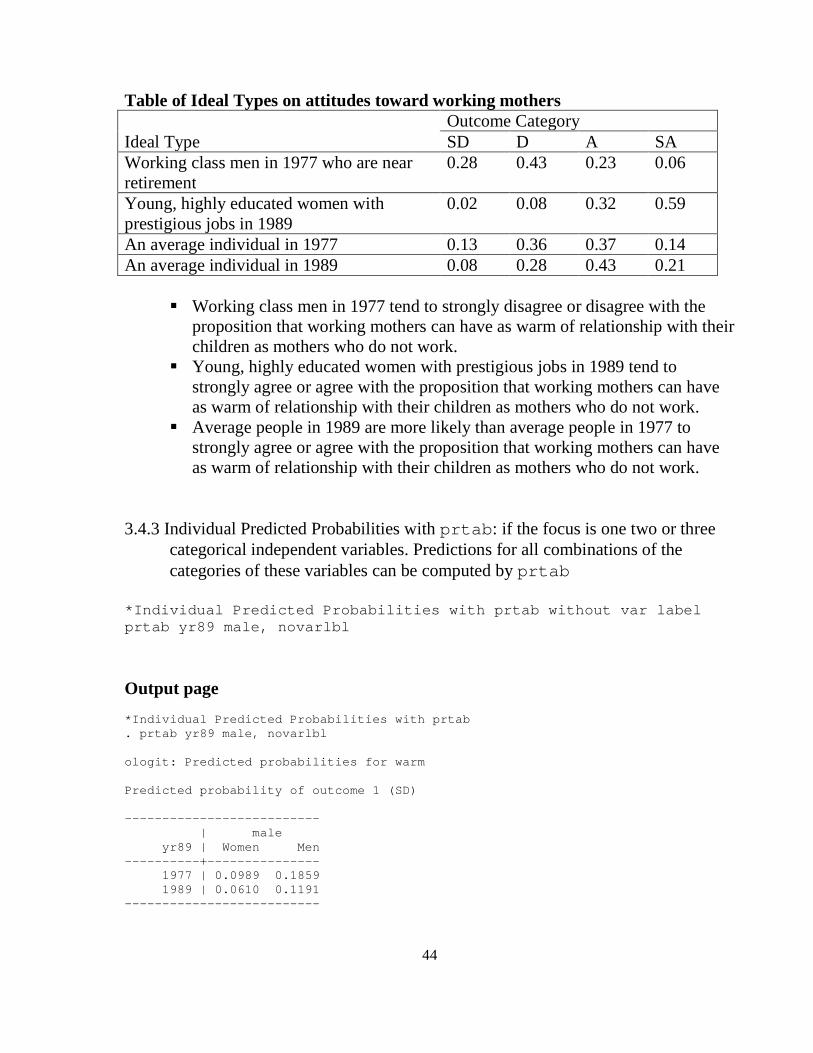
Table of Ideal Types on attitudes toward working mothers Outcome Category Ideal Type SD D A SA Working class men in 1977 who are near retirement

0.28 0.43 0.23 0.06

Young, highly educated women with prestigious jobs in 1989

0.02 0.08 0.32 0.59

An average individual in 1977 0.13 0.36 0.37 0.14 An average individual in 1989 0.08 0.28 0.43 0.21

Working class men in 1977 tend to strongly disagree or disagree with the proposition that working mothers can have as warm of relationship with their children as mothers who do not work.

Young, highly educated women with prestigious jobs in 1989 tend to strongly agree or agree with the proposition that working mothers can have as warm of relationship with their children as mothers who do not work.

Average people in 1989 are more likely than average people in 1977 to strongly agree or agree with the proposition that working mothers can have as warm of relationship with their children as mothers who do not work.

3.4.3 Individual Predicted Probabilities with prtab : if the focus is one two or three

categorical independent variables. Predictions for all combinations of the categories of these variables can be computed by prtab

*Individual Predicted Probabilities with prtab with out var label prtab yr89 male, novarlbl

Output page *Individual Predicted Probabilities with prtab . prtab yr89 male, novarlbl ologit: Predicted probabilities for warm Predicted probability of outcome 1 (SD) -------------------------- | male yr89 | Women Men ----------+--------------- 1977 | 0.0989 0.1859 1989 | 0.0610 0.1191 --------------------------

45

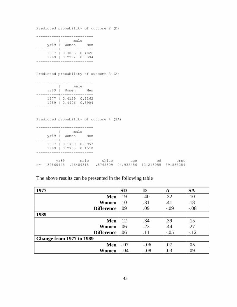
Predicted probability of outcome 2 (D) -------------------------- | male yr89 | Women Men ----------+--------------- 1977 | 0.3083 0.4026 1989 | 0.2282 0.3394 -------------------------- Predicted probability of outcome 3 (A) -------------------------- | male yr89 | Women Men ----------+--------------- 1977 | 0.4129 0.3162 1989 | 0.4406 0.3904 -------------------------- Predicted probability of outcome 4 (SA) -------------------------- | male yr89 | Women Men ----------+--------------- 1977 | 0.1799 0.0953 1989 | 0.2703 0.1510 -------------------------- yr89 male white age ed prst x= .39860445 .46489315 .8765809 44.935456 12. 218055 39.585259

The above results can be presented in the following table 1977 SD D A SA

Men .19 .40 .32 .10 Women .10 .31 .41 .18

Difference .09 .09 -.09 -.08 1989 Men .12 .34 .39 .15

Women .06 .23 .44 .27 Difference .06 .11 -.05 -.12

Change from 1977 to 1989 Men -.07 -.06 .07 .05

Women -.04 -.08 .03 .09

46

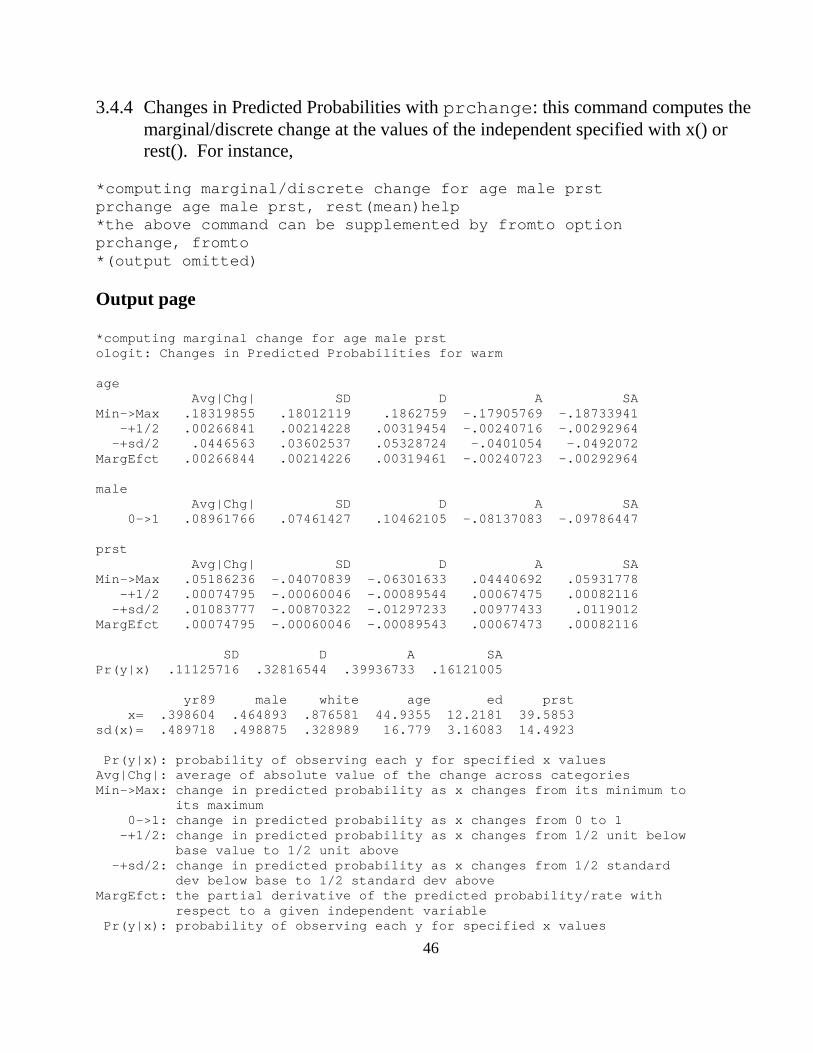
3.4.4 Changes in Predicted Probabilities with prchange : this command computes the marginal/discrete change at the values of the independent specified with x() or rest(). For instance,

*computing marginal/discrete change for age male pr st prchange age male prst, rest(mean)help

*the above command can be supplemented by fromto op tion prchange, fromto *(output omitted)

Output page *computing marginal change for age male prst ologit: Changes in Predicted Probabilities for warm age Avg|Chg| SD D A SA Min->Max .18319855 .18012119 .1862759 -.179 05769 -.18733941 -+1/2 .00266841 .00214228 .00319454 -.002 40716 -.00292964 -+sd/2 .0446563 .03602537 .05328724 -.04 01054 -.0492072 MargEfct .00266844 .00214226 .00319461 -.002 40723 -.00292964 male Avg|Chg| SD D A SA 0->1 .08961766 .07461427 .10462105 -.081 37083 -.09786447 prst Avg|Chg| SD D A SA Min->Max .05186236 -.04070839 -.06301633 .044 40692 .05931778 -+1/2 .00074795 -.00060046 -.00089544 .000 67475 .00082116 -+sd/2 .01083777 -.00870322 -.01297233 .009 77433 .0119012 MargEfct .00074795 -.00060046 -.00089543 .000 67473 .00082116 SD D A SA Pr(y|x) .11125716 .32816544 .39936733 .16121005 yr89 male white age ed prst x= .398604 .464893 .876581 44.9355 12.2181 39.5853 sd(x)= .489718 .498875 .328989 16.779 3.16083 14.4923 Pr(y|x): probability of observing each y for speci fied x values Avg|Chg|: average of absolute value of the change a cross categories Min->Max: change in predicted probability as x chan ges from its minimum to its maximum 0->1: change in predicted probability as x chan ges from 0 to 1 -+1/2: change in predicted probability as x chan ges from 1/2 unit below base value to 1/2 unit above -+sd/2: change in predicted probability as x chan ges from 1/2 standard dev below base to 1/2 standard dev above MargEfct: the partial derivative of the predicted p robability/rate with respect to a given independent variable Pr(y|x): probability of observing each y for speci fied x values

47

For a male respondent, the probability of strongly disagreeing is higher than a female respondent by .075, holding all other variables at their means For a standard deviation increase in age, the probability of disagreeing increase by .053, holding all other variables at their means Moving from the minimum prestige to the maximum prestige changes the predictability of strongly agreeing by .059, holding all other variables at their means

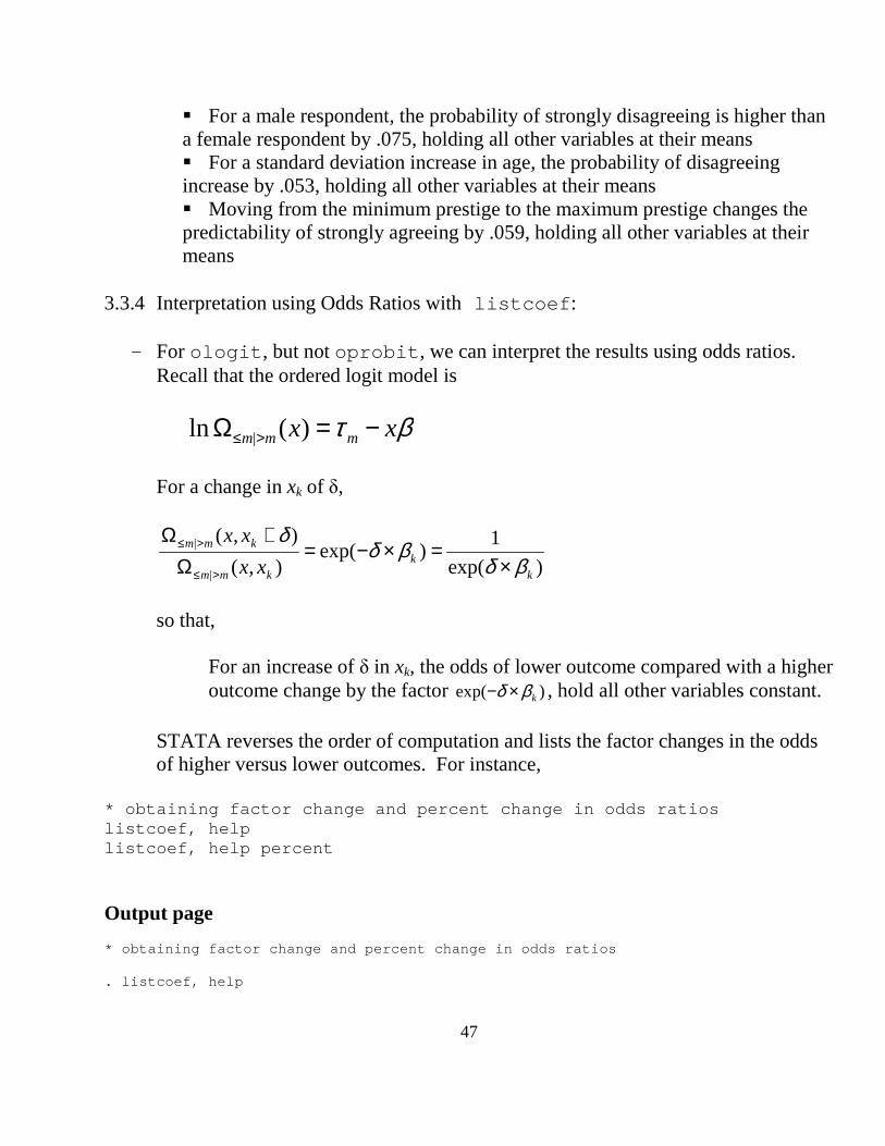
3.3.4 Interpretation using Odds Ratios with listcoef :

- For ologit , but not oprobit , we can interpret the results using odds ratios. Recall that the ordered logit model is

βτ xx mmm −=Ω >≤ )(ln |

For a change in xk of δ,

)exp(

1)exp(

),(

),(

|

|

kk

kmm

kmm

xx

xx

βδβδ

δ×

=×−=Ω

+Ω

>≤

>≤

so that,

For an increase of δ in xk, the odds of lower outcome compared with a higher outcome change by the factor )exp( kβδ ×− , hold all other variables constant.

STATA reverses the order of computation and lists the factor changes in the odds of higher versus lower outcomes. For instance,

* obtaining factor change and percent change in odd s ratios listcoef, help listcoef, help percent

Output page * obtaining factor change and percent change in odd s ratios . listcoef, help

48

ologit (N=2293): Factor Change in Odds Odds of: >m vs <=m --------------------------------------------------- ------------------- warm | b z P>|z| e^b e^bStdX SDofX -------------+------------------------------------- ------------------- yr89 | 0.52390 6.557 0.000 1.6886 1.2925 0.4897 male | -0.73330 -9.343 0.000 0.4803 0.6936 0.4989 white | -0.39116 -3.304 0.001 0.6763 0.8792 0.3290 age | -0.02167 -8.778 0.000 0.9786 0.6952 16.7790 ed | 0.06717 4.205 0.000 1.0695 1.2365 3.1608 prst | 0.00607 1.844 0.065 1.0061 1.0920 14.4923 --------------------------------------------------- ------------------- b = raw coefficient z = z-score for test of b=0 P>|z| = p-value for z-test e^b = exp(b) = factor change in odds for unit increase in X e^bStdX = exp(b*SD of X) = change in odds for SD i ncrease in X SDofX = standard deviation of X . listcoef, help percent ologit (N=2293): Percentage Change in Odds Odds of: >m vs <=m --------------------------------------------------- ------------------- warm | b z P>|z| % %StdX SDofX -------------+------------------------------------- ------------------- yr89 | 0.52390 6.557 0.000 68.9 29.2 0.4897 male | -0.73330 -9.343 0.000 -52.0 -30.6 0.4989 white | -0.39116 -3.304 0.001 -32.4 -12.1 0.3290 age | -0.02167 -8.778 0.000 -2.1 -30.5 16.7790 ed | 0.06717 4.205 0.000 6.9 23.7 3.1608 prst | 0.00607 1.844 0.065 0.6 9.2 14.4923 --------------------------------------------------- ------------------- b = raw coefficient z = z-score for test of b=0 P>|z| = p-value for z-test % = percent change in odds for unit increase in X %StdX = percent change in odds for SD increase i n X SDofX = standard deviation of X

The odds of having more positive attitudes towards working mothers are .48 times smaller for men than women, holding other variables constant (男性对职业妇女的亲子关系采较正面态度的胜算（或概率比）要比女性低 .48 倍). Or, the odds of having more positive attitudes towards working mothers are 52 percent smaller for men than women, holding other variables constant. For a standard deviation increase in age, the odds of having more positive attitudes decrease by a factor of .695, holding other variables constant.

49

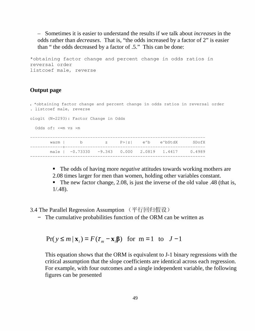
– Sometimes it is easier to understand the results if we talk about increases in the odds rather than decreases. That is, “the odds increased by a factor of 2” is easier than “ the odds decreased by a factor of .5.” This can be done:

*obtaining factor change and percent change in odds ratios in reversal order listcoef male, reverse

Output page . *obtaining factor change and percent change in odd s ratios in reversal order . listcoef male, reverse ologit (N=2293): Factor Change in Odds Odds of: <=m vs >m --------------------------------------------------- ------------------- warm | b z P>|z| e^b e^bStdX SDofX -------------+------------------------------------- ------------------- male | -0.73330 -9.343 0.000 2.0819 1.4417 0.4989 --------------------------------------------------- -------------------

The odds of having more negative attitudes towards working mothers are 2.08 times larger for men than women, holding other variables constant. The new factor change, 2.08, is just the inverse of the old value .48 (that is, 1/.48).

3.4 The Parallel Regression Assumption （平行回归假设）

− The cumulative probabilities function of the ORM can be written as

1 to1mfor )()|Pr( −=−=≤ JFmy imi βxx τ

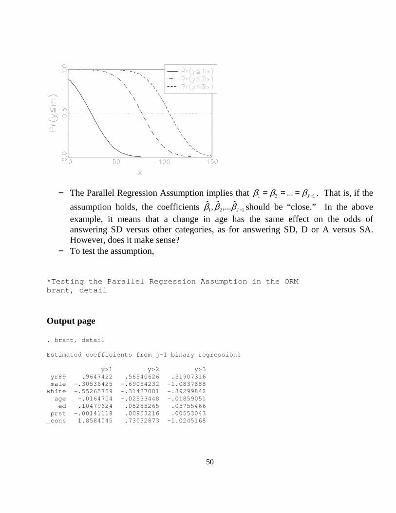
This equation shows that the ORM is equivalent to J-1 binary regressions with the critical assumption that the slope coefficients are identical across each regression. For example, with four outcomes and a single independent variable, the following figures can be presented

50

− The Parallel Regression Assumption implies that 121 ... −=== Jβββ . That is, if the

assumption holds, the coefficients 121ˆ,...ˆ,ˆ

−Jβββ should be “close.” In the above example, it means that a change in age has the same effect on the odds of answering SD versus other categories, as for answering SD, D or A versus SA. However, does it make sense?

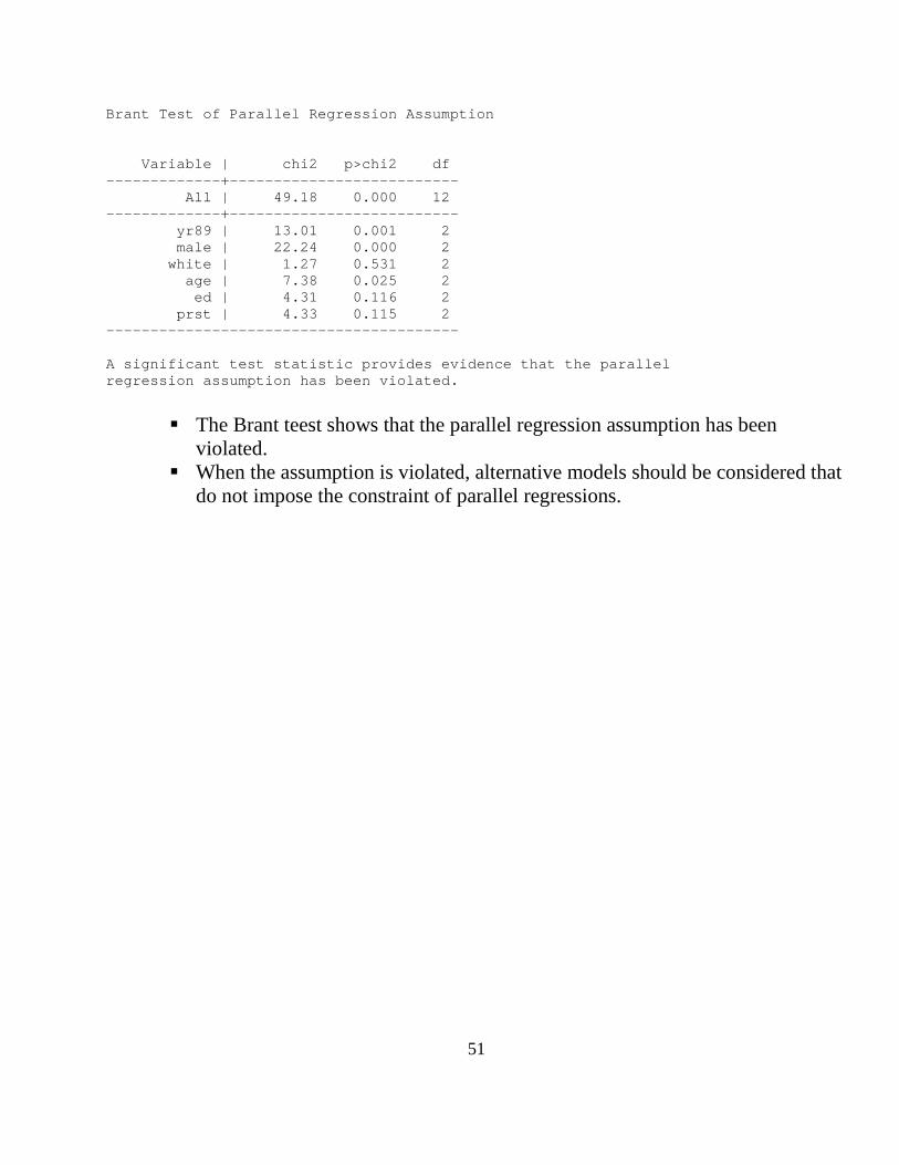
− To test the assumption, *Testing the Parallel Regression Assumption in the ORM brant, detail

Output page . brant, detail Estimated coefficients from j-1 binary regressions y>1 y>2 y>3 yr89 .9647422 .56540626 .31907316 male -.30536425 -.69054232 -1.0837888 white -.55265759 -.31427081 -.39299842 age -.0164704 -.02533448 -.01859051 ed .10479624 .05285265 .05755466 prst -.00141118 .00953216 .00553043 _cons 1.8584045 .73032873 -1.0245168

51

Brant Test of Parallel Regression Assumption Variable | chi2 p>chi2 df -------------+-------------------------- All | 49.18 0.000 12 -------------+-------------------------- yr89 | 13.01 0.001 2 male | 22.24 0.000 2 white | 1.27 0.531 2 age | 7.38 0.025 2 ed | 4.31 0.116 2 prst | 4.33 0.115 2 ---------------------------------------- A significant test statistic provides evidence that the parallel regression assumption has been violated.

The Brant teest shows that the parallel regression assumption has been

violated. When the assumption is violated, alternative models should be considered that

do not impose the constraint of parallel regressions.