Ms

JHa

b

c

d

e

a

A

KESINCS

1

ipipWeabtto

(

wi

h0

Social Networks 54 (2018) 196–208

Contents lists available at ScienceDirect

Social Networks

journa l homepage: www.e lsev ier .com/ locate /socnet

odels, methods and network topology: Experimental design for thetudy of interference

ake Bowers a,∗, Bruce A. Desmarais b, Mark Frederickson a, Nahomi Ichino c,suan-Wei Lee d, Simi Wang e,1

Departments of Political Science and Statistics, University of Illinois at Urbana-Champaign, United StatesDepartment of Political Science, Pennsylvania State University, United StatesDepartment of Political Science, University of Michigan, United StatesDepartment of Sociology, University of Nebraska-Lincoln, United StatesDepartment of Applied Mathematics, University of North Carolina at Chapel Hill, United States

r t i c l e i n f o

rticle history:

eywords:xperimental designpillovernterferenceetworksausal inferencetatistical power

a b s t r a c t

How should a network experiment be designed to achieve high statistical power? Experimental treat-ments on networks may spread. Randomizing assignment of treatment to nodes enhances learning aboutthe counterfactual causal effects of a social network experiment and also requires new methodology (ex.Aronow and Samii, 2017a; Bowers et al., 2013; Toulis and Kao, 2013). In this paper we show that the wayin which a treatment propagates across a social network affects the statistical power of an experimen-tal design. As such, prior information regarding treatment propagation should be incorporated into theexperimental design. Our findings justify reconsideration of standard practice in circumstances whereunits are presumed to be independent even in simple experiments: information about treatment effects

is not maximized when we assign half the units to treatment and half to control. We also present anexample in which statistical power depends on the extent to which the network degree of nodes is cor-related with treatment assignment probability. We recommend that researchers think carefully aboutthe underlying treatment propagation model motivating their study in designing an experiment on a network.

. Introduction

We consider the problem of designing experiments to causallydentify propagation on networks. In a simple experiment on inde-endent units with complete randomization to two treatment arms,

t is often assumed that one should assign half of the experimentalool to treatment and half to control (Gerber and Green, 2012).2

hen treatment given to one unit may affect another unit, how-ver, we show (in a simulation study using a realistic networknd realistic model of network treatment propagation) that it maye better to assign less than half of the pool to treatment from

he perspective of statistical efficiency. The intuition is simple: ifreatment spreads rapidly across a network, then comparisons ofutcomes between treated and control units will become very small

∗ Corresponding author.E-mail addresses: jwbowers@illinois.edu (J. Bowers), bdesmarais@psu.edu

B.A. Desmarais).1 Authors listed alphabetically.2 Technically speaking, the 50/50 treatment allocation is optimal for precisionhen randomization is complete at the unit-level and outcomes have equal variance

n both treated and control groups.

ttps://doi.org/10.1016/j.socnet.2018.01.010378-8733/Published by Elsevier B.V.

Published by Elsevier B.V.

or even vanish as the control units to which the treatment spreadwill act just like treated units. Thus, one might field a very effec-tive experiment, perhaps an experiment in which controls race toget access to the treatment or treated units spread the informa-tion or other active ingredient far and wide, but be unable to detecteffects if everyone in the whole network reveals the same outcomewhether or not they were assigned to treatment. The simulationsthat we show here confirm this intuition, but also reveal a trade-offbetween ability to detect the direct effects of treatment assignmenton the units initially assigned to treatment and the ability to detectthe indirect or network mediated effects of the treatment as it prop-agates to control units. One point that we emphasize in this paperis that the way in which a treatment propagates matters a greatdeal as we think about how to design experiments on networks.

In fields across the social and physical sciences, there is con-siderable and growing interest in understanding how featurespropagate over the vertices (i.e., nodes) in a graph (i.e., network) viathe graph topology. Furthermore, precise questions about causal

peer, spillover and propagation effects are becoming more com-mon. Recent theoretical developments highlight the barriers to theidentification of causal peer/contagion effects in networks withnon-randomized, or observational, data (Lyons, 2011; Shalizi and

etwo

TipB2cgms

ttathwargoldsbtHaaTdrs

dAEstdha—devflwdb

(rM

ef2a2I

smio

J. Bowers et al. / Social N

homas, 2011). Several recent papers have employed random-zed experimental designs to facilitate the identification of causaleer effects (Aral and Walker, 2011; Ostrovsky and Schwarz, 2011;apna and Umyarov, 2015; Bond et al., 2012; Ichino and Schündeln,012; Nickerson, 2008). For example, Ichino and Schündeln (2012)onduct a field experiment during a national election in Ghana toauge how voter registration responds to the placement of electiononitors at registration workstations — an effect that is hypothe-

ized to spread geographically through the road network.Recent methodological work enables scholars to make statis-

ical inferences about peer effects or global average effects whenhe topology of a network is known (Bowers et al., 2013; Aronownd Samii, 2017a; Eckles et al., 2017; Toulis and Kao, 2013).3 Ashe ability to pose questions of spillover has increased, researchersave begun to address how well these methods work, particularlyith respect to statistical efficiency. Eckles et al. (2017) show that

graph cluster randomization design — where groups of nodes areandomized to treatment together — reduces bias in estimates oflobal average treatment effects with relatively little cost in termsf statistical power. Baird et al. (2017) derive the efficiency calcu-

ations for estimates of average spillover effects for randomizationesigns in which isolated groups of nodes are randomized first to aaturation proportion — the proportion of units within the group toe randomized to treatment — and then within group randomiza-ion proceeds according to the first level randomization. Hirano andahn (2010) derive efficiency calculations regarding cluster-wisend within-cluster treatment proportions for estimates of directnd indirect effects in two-level cluster randomization designs.hese approaches answer important questions about particularesigns; however, there is still a need to address how to designandomization schemes to increase the statistical power to detectpecific forms of network mediated peer effects.

In this project we consider the performance of different ran-omization designs using the methods of Bowers et al. (2013) andronow and Samii (2017a) under different models of propagation.ach of the methods we consider depends upon a typology of expo-ure conditions based on the treatment status of each node andhe topology of the graph. For example, a node could be treatedirectly by an experimenter, isolated from treatment (i.e., severalops away from any treated nodes) or exposed to the treatmentt one degree of separation by virtue of the network relationship

without control by the experimenter. The performance of ran-omized experimental designs on networks depends on (1) thexposure conditions of theoretical interest (say, direct treatmentersus indirect treatment; or more generally some propagationow parameter), (2) the topology of the network, (3) the ways inhich the propagation model affects nodes in each exposure con-

ition, and (4) the exposure condition distribution as determinedy the randomization design.4

To anchor our interest in interference, consider Coppock’s

2014) recent replication of Butler et al. (2011). Butler et al. (2011)un a field experiment that is focused on a special session of the New

exico legislature that was called to consider a specific budgetary

3 For now, we set to the side the work on identifying how much of a total averageffect can be attributed to mechanisms other than direct treatment assignment —or example, the work on spillovers and indirect effects (Sinclair et al., 2012; Sinclair,011; Nickerson, 2008, 2011; Hudgens and Halloran, 2008; Sobel, 2006; Tchetgennd VanderWeele, 2010; VanderWeele, 2008, 2010, 2011; VanderWeele et al., 2011,012; VanderWeele and Tchetgen, 2011; Miguel and Kremer, 2004; Chen et al., 2010;

chino and Schündeln, 2012).4 We direct readers to Basse and Airoldi (2015) for a methodological investigation

imilar to ours. They consider the problem of designing a randomized experiment toinimize estimation error when outcomes are correlated on a network. Their focus

s, however, on estimating the direct effects of treatment, not on identifying indirectr propagation effects.

rks 54 (2018) 196–208 197

question. The field experiment was designed to test the influence ofproviding information about constituents’ preferences on legisla-tors’ votes. Constituents across the state were first surveyed on thebudget question on which their legislators would be voting. Butlerand Nickerson sent district-specific results to randomly selectedmembers of the legislature. They found that providing informa-tion about constituents’ preferences shifted legislators’ votes in thedirection of those preferences. Coppock (2014, pp. 159–160) notesthat,

“The estimates of responsiveness recovered by Butler et al.(2011) rely on an assumption of non-interference (Cox 1958;Rubin, 1980): Legislators respond only to their own treatmentstatus and not to the treatment status of others. This assumptionrequires that legislators not share treatment information withone another, which is at odds with the observation by Kingdon(1973, p. 6) that legislatures are information-sharing networks.”

In replicating Butler et al. (2011), Coppock (2014) specifies amodel for the propagation of effects that spread through a networkbetween legislators defined by ideological similarity. Accountingfor the fact that the treatment assigned to one legislator had effectson other legislators, Coppock (2014) estimates that the experimentshifted nearly twice as many votes in the legislature as was origi-nally estimated by Butler et al. (2011).5

In what follows, we study the problem of causal inference giventreatment propagation in the context of a fixed graph topology anda single round of randomized treatment and by a single roundof response measurement. We review methods that have beenproposed in the literature for analyzing single-round (pre versuspost), fixed graph experimental data; and also review the sub-stantive experimental applications that have used such designs.We then conduct a simulation study motivated by the registrationmonitor randomization in Ichino and Schündeln (2012), using theGhanaian network of roads between voter registration stations asa realistic moderate sized graph.6 In the simulation study, we con-sider the performance of alternative experimental designs that varythe treatment probability: the number of nodes assigned to initialtreatment, who is treated: the association between treatment prob-ability and node degree (i.e., a node’s number of ties), and how theyare treated: different parameterizations of the propagation model.

1.1. Statistical inference for propagated causal effects

We consider two general approaches to statistical inferenceabout causal effects when those effects may propagate through anetwork. The flexible approach developed by Bowers et al. (2013)is a hypothesis testing framework designed to evaluate whetherdifferences between the treatment and control groups are moreeffectively characterized by one model of treatment effects, whichcan include propagation effects, than another model. Bowers et al.(2013) focus on a natural sharp null model of no treatment effects(i.e., stochastic equivalence across all experimental conditions).The null distribution is derived exactly or generated approximately

through repeated computations of the test statistic using permuta-tions in which the treatment vector is re-randomized accordingto the experimental design, and the hypothesized effects of thepropagation model are removed. There are two highly appealing

5 Coppock (2016) later shows that the test statistic and research design wasunderpowered to detect this effect.

6 Ichino and Schündeln (2012) did not use the road network in their paper, butinstead focused on estimating average spillover effects within radii of 5 km and10 km following the multi-level experimental design of Sinclair et al. (2012). We usethe road network to provide us with a realistic network for use in our simulationsstudying the power of different randomization allocation plans.

1 etwo

pe(tmno

Tearbcabtotparddnat(dbdatatWtc

orlsp(ee(o(taateac(dl

(eKas

98 J. Bowers et al. / Social N

roperties of this approach. First, any test statistic, including gen-ral distributional comparisons such as the Kolmogorov–SmirnovKS) test statistic, can be used to evaluate the differences betweenreatment and control. Second, the approach can accommodate any

odel of treatment effects on a network, as the methodology doesot require any form of independence assumption or the derivationf an estimator for the model parameters.

The methods developed by Aronow and Samii (2017a) andoulis and Kao (2013) compliment those proposed by Bowerst al. (2013) in that they propose methods for estimating aver-ge causal peer effects. Aronow and Samii (2017a) developsandomization-based methods and Toulis and Kao (2013) developsoth randomization and model-based approaches to estimatingausal peer effects. In both Aronow and Samii (2017a) and Toulisnd Kao (2013), the target estimate is the average differenceetween nodes in different network/treatment exposure condi-ions. Aronow and Samii (2017a) do not stipulate a constrained setf conditions, but present methods that can be applied to any par-ition of nodes into network/treatment exposure conditions. Theyresent an example in which nodes in a graph are directly treatednd assume that treatment can only propagate one degree, whichesults in four conditions: control, which are nodes that are notirectly assigned treatment and are not tied to any treated nodes;irect, which are nodes that are treated and not tied to any treatedodes, direct + indirect, which are nodes that are directly treatednd are tied to treated nodes; and isolated direct, which are nodeshat are untreated and are tied to treated nodes. Toulis and Kao2013) define k-level treatment of a unit as (1) a unit not receivingirect treatment, and (2) having exactly k directly treated neigh-ors. A k-level control is any vertex with at least k neighbors whoid not (1) receive direct treatment and (2) is not connected tony vertices who were directly treated. These approaches assumehat the researcher is interested in specific comparisons of averagesnd require that the researcher articulate mechanisms by whichhe probability of exposure to treatment may differ across units.

hen networks are fixed prior to treatment and the randomiza-ion mechanism known, the probability of exposure can be directlyomputed.

Both Aronow and Samii (2017a) and Toulis and Kao (2013) rec-gnize the unique challenges that arise in the context of inferenceegarding response to network/treatment exposure conditions. Theimitations are based in the topology of the graph. Since most expo-ure conditions of interest in the context of interference involve theosition of a node in a network, under most randomization designse.g., uniform random assignment to treatment), each node is notqually likely to be assigned to each exposure condition. Take thexample of 2-level exposure in the framework of Toulis and Kao2013). A node with only one partner would have zero probabilityf being assigned to the 2-level treatment group. Aronow and Samii2017a) do not discuss this issue at length, but imply a limitation inhe derivation of their Horvitz-Thompson type estimators (Horvitznd Thompson, 1952). The estimators they define require that thenalyst be able to calculate the probability �i(dk), the probabilityhat node i is in exposure condition dk and that 0 < �i(dk) < 1 forach node i. This means that the framework proposed by Aronownd Samii (2017a) cannot be applied to the comparison of exposureonditions to which all nodes cannot be assigned. Toulis and Kao2013) are more explicit in their discussion of this limitation. Theyefine a causally valid randomization design to be one in which at

east one node is k-level treated and one is k-level controlled.In the analysis that follows, we consider Aronow and Samii

2017a) and Bowers et al. (2013) approaches to inference with

xperiments on networks. The methods proposed by Toulis andao (2013) are very similar to those of Aronow and Samii (2017a),nd their concepts of k-level treated and k-level controlled can beeen as special cases of the exposure conditions defined in Aronow

rks 54 (2018) 196–208

and Samii (2017a). Furthermore, the methods of Aronow and Samii(2017a) have the added advantage of adjusting the treatment effectestimates (and variance estimates) for the unequal exposure condi-tion probabilities. These Horvitz-Thompson type adjustments willcorrect for any associations between exposure condition probabil-ities and potential outcomes (e.g., higher degree nodes may exhibithigher baseline response values and be more likely to be indirectlyexposed to treatment through propagation).

2. Design as a function of graph topology

Walker and Muchnik (2014) reviews several applications ofexperiments in networked environments — including studies thatare not focused on propagation — and outline several of the fun-damental challenges to designing experiments on networks. Theysummarize the problem of design in experiments on networks suc-cinctly (p. 1949):

“The natural connectivity of our world does not only present achallenge to the conventional paradigm of experimental design,but also reveals opportunities to leverage connectivity throughthe creation of novel treatment mechanisms that incorpo-rate both experimental subjects and the connections betweenthem.”

The practical implication of the dependence between subjectsvia the network is that efficient experimental designs will accountfor graph topology. The treatment assignment algorithms pre-sented in Toulis and Kao (2013) render a clear picture of how theimportance of network structure can complicate design. Consid-ering the problem of assuring that sufficient numbers of verticesend up in the k-treated and k-controlled designs, Toulis and Kao(2013) present sequential randomization designs that assure thatfixed numbers of vertices are assigned to the groups under com-parison: for example, if a researcher desires to know the effectof the treatment on nodes having 2 directly connected neigh-bors in the network, a design should ensure enough nodes withdegree 2 assigned treatment versus not are assigned treatment.Though powerful in their ability to control the distribution ofvertices across exposure conditions, the complex sequential ran-domization algorithms proposed by Toulis and Kao (2013) makeclosed-form calculation of the probability of exposure conditionassignment intractable in most cases, which may be why they donot derive their estimators using Horvitz-Thompson adjustmentssuch as those in Aronow and Samii (2017a). An example of a non-sequential randomization design for which it is straightforward toderive the Horvitz-Thompson weights is one in which the prob-ability of treatment is biased with respect to vertex degree (e.g.,disproportionately treating higher degree vertices). To provide anintuitive example regarding why it might be advantageous to treathigh degree vertices at a greater rate than low degree vertices; sup-pose the researcher is interested in comparing nodes isolated fromtreatment (e.g., more than two degrees from any directly treatednode) to nodes that are adjacent to a treated node, but are notdirectly treated. Each node that is directly treated is removed fromboth exposure conditions of interest, so there is an incentive to treata small proportion of nodes. However, if too few nodes are treated,there will be too few nodes in the adjacent-to-treated condition.By focusing the treatment on higher degree nodes, it takes fewerdirectly treated nodes to accomplish a sizable sample of adjacent-to-treated nodes. Depending upon the structure of the network

and the mechanism by which treatment can propagate, there maybe a considerable gain in statistical power from biasing treatmenttowards high degree nodes, as compared to uniform assignment totreatment.

J. Bowers et al. / Social Networks 54 (2018) 196–208 199

F rk can( cationt

dncnte

•

•

•

•

editwtfsctafol

tdtmeiil

2

Zwtm

ig. 1. Example illustrating how simple random treatment assignment on a netwoa) gives an example grid network of twelve nodes. Panel (b) gives the average allohree (i.e., 25%) and six (i.e., 25%) nodes.

Consider a simple example that illuminates how the ability toraw comparisons in experiments on networks can depend sig-ificantly on design decisions. In this example, an experiment isonducted by allocating a binary treatment in a network of twelveodes connected on a 3 × 4 grid (illustrated in Fig. 1(a)). Supposehe experimenter is planning to draw some comparisons across fourxposure conditions of nodes:

Isolated Control: Control nodes that are not adjacent to any treatednodes.Isolated Treated: Treatment nodes that are not connected to anytreated nodes.Exposed Control: Control nodes that are adjacent to at least onetreated node.Exposed Treated: Treated nodes that are adjacent to at least onetreated node.

Now consider two designs for assigning nodes to treatment. Inach design, the set of treated nodes is selected uniformly at ran-om from the set of twelve nodes. In the first design, treatment

s assigned to 25% of the nodes (i.e., three). In the second design,reatment is assigned to 50% of the nodes (i.e., six). In Fig. 1(b)e present the average percentage of nodes allocated to each of

he exposure conditions. Generally speaking, the allocation to theour conditions differs dramatically between the two designs. Morepecifically, under the design in which 50% of the nodes are allo-ated to treatment, fewer than 15% of the nodes are isolated fromreatment, on average. If the experimenter is planning to conductnalysis that depends on the number of nodes that are isolatedrom treatment, the design in which treatment is assigned to 50%f the nodes will likely result in very imprecise estimates and/or

ow power statistical tests.This simple example illustrates two points upon which we build

hroughout the paper. First, the power of a network experimentepends, in complex ways, on the structure of the network, thereatment assignment distribution, and the effects of the treat-

ent — both direct and indirect. Second, if the precision in thestimates/analysis depends upon the number of subjects that aresolated from treatment, following the common practice of allocat-ng half the experimental subjects to treatment may result in veryow power/precision.

.1. Design is dependent on a model of propagation

Let Zi = 1 if subject i is assigned to the treatment condition and

i = 0 if i is assigned to control. In the classical experimental frame-ork, a counterfactual causal effect for a person i is defined through

he comparison of that person’s outcome, Yi(Zi = 1) under one treat-ent to that same person’s outcome under a different treatment

lead to very different allocations of nodes to network exposure conditions. Panel across exposure conditions given simple random assignment to treatment of both

Yi(Zi = 0), given at the same moment in time (Neyman, 1990; Rubin,1980; Holland, 1986). If potential outcomes under different treat-ments differ, Yi(Zi) /= Yi(Z ′

i) for Zi /= Z ′

i, we say the treatment had an

effect. Implicit in this comparison for a single person is the pre-sumption that subject i’s outcome only depends on i’s treatmentstatus Zi and not on any other Zj — that there is no interfer-ence between the treatment or outcomes of person i and thoseof any other person. Such implicit assumptions are incompatiblewith the goals of researchers seeking to understand the importantcausal role played by networks in real world processes. Analysis ofexperiments on social networks cannot assume away interference,especially if a scholar desires to learn about propagation processes.However, once the assumption of no interference is relaxed, a theo-retical model of interference represents a valuable tool to guide thesearch for propagation’s footprint and to calibrate the experimentaldesign. One method to deal with interference would be to specifythe potential outcomes for each unit as a function of the entire treat-ment assignment to all nodes (Bowers et al., 2013). Such a method ispowerful, but it can be theoretically demanding to specify a modelfor each unit’s outcome. As Aronow and Samii (2017b) show, it isnot strictly necessary to assume a theoretical model of interferencein order to identify interference effects by instead looking at broadclasses of interference. Nevertheless, in both scenarios, a theoreticalmodel of interference is needed to identify the interference effectsfor which the researcher intends to test, which, in turn, can informthe design of the experiment.

While having differing statistical motivations, the methods ofAronow and Samii (2017a) and Bowers et al. (2013) both requirethat the researcher draw upon a theoretical model of interferenceto properly analyze the outcome Y. In Aronow and Samii (2017a), amodel of interference must be used to identify the exposure condi-tions (e.g., adjacent to a treated unit, 2 degrees of separation froma treated unit, etc.) to be compared in the study. The model usedwith the methods of Aronow and Samii (2017a) need not provideprecise predictions about to which nodes the treatment will prop-agate and how, but the model must be complete enough to identifythe groups of nodes for which different potential outcomes will beobserved under a given direct treatment assignment regime. Forthe methods proposed by Bowers et al. (2013), a precise analyticmodel of interference must be specified. The approach adjusts theobserved data by removing effect of the treatment as specified bya parametric model of effects, including both direct and indirecteffects. If the model captures the true treatment effects, outcomeand treatment assignment should be statistically independent forany test statistic. This statistical independence can be tested by per-

muting the treatment assignment labels, computing a test statisticfor each assignment, and comparing the test statistic of the adjusteddata to the distribution of test statistics. As the adjusted data mustbe constructed from a model, it is not possible to use the meth-

2 etworks 54 (2018) 196–208

oi

trvmlmdH((Dpt1bwF

3

uSupmicuIitatstiroccrd

3

tZuoYmt

i

ibmp

Table 1Adjacency matrix of a simple 6 node network with 4 edges.

A B C D E F

A 0 1 1 0 0 0B 1 0 0 0 0 0C 1 0 0 0 0 1

00 J. Bowers et al. / Social N

ds of Bowers et al. (2013) without specifying the precise role ofnterference in the study.

The need to specify a model of propagation in order to iden-ify an efficient experimental design leads us to question whereesearchers might start in developing such models. There is aibrant literature, primarily in the fields of physics and appliedathematics, on graph dynamics, that provides several excel-

ent starting points for analytical models of propagation. Theseodels include the susceptible-infected-recovered disease epi-

emic models (Kermack and McKendrick, 1927; Anderson, 1982;ethcote, 2000; Daley and Gani, 2005), the Bass Diffusion Model

Bass et al., 1994; Lenk and Rao, 1990) and the Hopfield networkHopfield, 1982) and the voter model (Clifford, 1973; Liggett, 1997;urrett and Kesten, 1991). In the simulation study that follows, weresent and use a variant of the Ising model, a model that con-ains several of those mentioned above as special cases (Gallavotti,999). The Ising model is a general formulation for stochasticinary-state dynamics. The classic Ising model has been used quiteidely to characterize opinion dynamics (e.g., Vazquez et al., 2003;

ortunato, 2005; Sousa et al., 2008; Biswas and Sen, 2009).

. Simulation study

In what follows we conduct a simulation study in which we eval-ate the statistical power of the methods proposed by Aronow andamii (2017a) and Bowers et al. (2013). The objective of this sim-lation study is to demonstrate that the statistical power of theserocedures depends upon design parameters that are intuitivelyeaningful in the context of propagation, and that power is max-

mized at design parameters that differ considerably from thoseommonly used in experiments without interference — randomniform division of the sample into half control and half treatment.7

t is outside the scope of the current study to compare the mer-ts of the methods proposed by Aronow and Samii (2017a) withhose proposed by Bowers et al. (2013): further, we see the twopproaches as complementary in the same way that hypothesisesting and estimation complement one another. We hope that ourimulation will illustrate the importance and feasibility of simula-ion analysis for parameterizing designs for studies of propagationn networks. Throughout this simulation we use the Ghana voteregistration station network from Ichino and Schündeln (2012) asur example network. We create a network from the map of roadsonnecting the registration stations. Two registration stations areonsidered to be tied if they are within 20 km of each other on theoad network. This results in a network with 868 vertices, and aensity of 2.2%. The network is depicted in Fig. 5.8

.1. Simulation parameters and definitions

We denote the treatment assigned to vertex i as Zi ∈ {0, 1} andhe vector of treatment assignments to all vertices as Z = (Z1, . . .,n)T. The fixed potential outcome of vertex i that would be shownnder treatment vector Z is denoted Yi(Z). Under the sharp null

f no treatment effect, all potential outcomes are equal; Yi(Z) =i(Z

′) = Yi({Zi = 1, Z−i}) = Yi({Zi = 0, Z′−i}) ∀Z /= Z′ and where −i

eans “all vertices not i”. Yit(Dit) is the potential outcome of ver-ex i at time t under exposure condition Dit. The exposure condition

7 See Gerber and Green (2012, Chap. 3) for one example of a discussion about why,n general, a half/half treatment/control split maximizes power.

8 We depart from the details and substantive aims of Ichino and Schündeln (2012)n that we replace a road network with a graph that creates direct connectionsetween nodes. This enables us focus on network propagation rather than, say, theovements of actual human agents on road, or on the specifics of the study of the

ropagation of voter registration fraud in Ghana.

D 0 0 0 0 1 0E 0 0 0 1 0 0F 0 0 1 0 0 0

indicates a mapping of the graph topology and Z into the categoriesof exposure defined by the researcher (e.g., directly treated andnot tied to any directly treated vertices, not directly treated andadjacent to at least one directly treated node).

To motivate this discussion, and introduce the primary statis-tical method, we introduce a toy example using a simpler modeland test statistic than will be later employed. The primary goal ofthis toy example is demonstrate how the power, the probabilityof rejecting a false null hypothesis, of the statistical approach candepend heavily on the treatment assignment mechanism, the net-work, and the interaction of these two features in generating theobserved outcome. Table 1 shows the adjacency matrix of this sim-ple network. We label this network S. Additionally, for each nodewe have a background covariate x = (2.4, 0.6, 2.2, 0.9, 0.4, 0)′. Thecovariate and the network combine with the treatment assignmentZ in two outcome models:

Y(Z) = x + �Z (1)

Y(Z) = x + �Z + (1 − Z)�I(SZ > 0) (2)

In the first model, as each node’s outcome depends only on itsown treatment status, this model involves no spillover. The sec-ond model, on the other hand, treated units share their benefitwith any untreated neighbors. For simplicity, we fix the true � at1 in both models. To contrast different assignment mechanisms,we consider two treatment assignment mechanisms: assign twounits to treatment, four to control (“unbalanced”); three units totreatment, three to control (“balanced”). For each possible treat-ment strategy, we can enumerate all possible treatment allocation(15 for the unbalanced case and 20 for the balanced case). For eachallocation, we can generate the Y that would be observed if � = 1. Foreach of these observed Y, we then apply the randomization infer-ence procedure, using a squared t-statistic, to compute p-valuesfor the (false) hypothesis that treatment had no effect (i.e., � = 0).This results in a p-value that would be observed for each possiblerandomization. For a given ˛-level, the randomization method thathas more p-values less than ̨ has higher power.

Fig. 2 compares the two assignment methods when spilloveris and is not present with respect to power, as a function of theselected ˛-level. As the figure shows, in the absence of spillover,the balanced design almost always possess better power charac-teristics than the unbalanced design. As power is a function ofp-values generated for each randomization, it can be useful toconsider the mean p-value of the sharp null hypotheses for thesedifferent methods, where lower mean p-values correspond to morepower. Overall, for the balanced design the average p-value with-out spillover was 0.4 while for the unbalanced design had meanp-values of 0.493. Conversely, when spillover is present the unbal-anced design generally has superior power to the balanced design,with an overall mean of 0.547 compared to 0.56 for the balanceddesign. While the difference between the p-values for the spillovermodel is small, it is important to note that conventional wisdom

holds that balanced designs always possess superior power advan-tages. When spillover is present, however, this is not universallytrue. In some situations, when spillover is present, unbalancedassignment can increase statistical efficiency.

J. Bowers et al. / Social Networks 54 (2018) 196–208 201

Fig. 2. Proportion of randomizations that would reject the null hypothesis that � = 0when � = 1 (“power”) of the two assignment methods (assigning 2 out of 6 or 3 outorag

smugtZti

wopiitmta

uiZZ

f 6 subjects to treatment) as a function of the ˛-level employed. The top panelepresents the case of the model of direct effects only, while the lower panel addsn indirect effect for any node that has at least one treated neighbor. The verticalray line is at ̨ = 0.10.

To investigate this phenomenon in a more realistic setting, in theubsequent simulations we employ a much richer model of treat-ent effects as well as test statistics that have proven themselves

seful in network settings. The model we use for treatment propa-ation in our simulations is a variant of the Ising Model. The initialreatment assignment of each vertex is drawn independently fromi ∼ Bernoulli(˛). The infection probability — the probability thatreatment “infects,” or propagates to, a control vertex — at eachteration of propagation is

1

1 + exp(

2F (ki − 2mi)

) ,

here k is number of (directly adjacent) neighbors, m is the numberf previously exposed neighbors (0 ≤ mi ≥ M), F is a “temperature”arameter that governs the extent to which the propensity to be

nfected depends on the infection rate among i’s neighbors. Wenitialize the model by assigning treatment (t = 0), and then we runhe propagation model for just one time period (t = 1). The Ising

odel controls actual infection after an experimenter assigns Zi at = 0. By only producing one iteration of the model, we thus onlyllow interference at one step or degree in the network.

We specify the potential outcomes of the vertices in our sim-

lation according to the following scheme depending upon the

nfection status at a given time point. We denote this by Y(Zi,t=0,i,t=1), in which Zi0 ≡ Zi,t=0 indicates i’s initial treatment status andi1 indicates whether treatment propagates to i at time 1. In the sim-

Fig. 3. Illustration of exposure conditions for a subgraph of the Ghana road network.One draw from the Ising propagations with pr(Zi = 1) ∼ Bernoulli(. 15) for t ∈ {0, 1}and Temperature = 10.

ulation study we consider both multiplicative and additive effects,and propagation models in which treatment propagates stochasti-cally according to the Ising model, and propagates with certaintyfrom directly treated units to their direct neighbors. We generatea baseline (pre-treatment) response Y(0, 0) ∼ U(0, 1) to representthe state of the graph in the absence of any experiment. Our multi-plicative treatment effect model changes the baseline in the same,multiplicative, way regardless of the time or manner of “infection”(directly assigned by researcher or propagated from a neighbor),and Y(1, 0) = Y(0, 1) = �Y(0, 0). In the additive treatment effect modelY(1, 0) = Y(0, 1) = � + Y(0, 0). We consider values of � ∈ {0.26, 0.63},which correspond to approximately one and two standard devi-ation shifts in the mean of a standard uniform random variable,and simulate 1000 treatment propagation and outcome sets at eachcombination of F ∈ {0, 10, . . ., 100} and ̨ ∈ {0.05, 0.10, . . ., 0.50}.

3.2. Application of inference methods

Aronow and Samii’s (2017a) method requires that we defineexposure conditions (which include assignment to treatment andalso the probability of exposure to a treatment via the network). Wedefine the exposure conditions with respect to what a researcherwould be able to observe from the experimental design, assum-ing the network were observed, and the response. Importantly, indefining the exposure conditions of interest, we assume that theresearcher does not exactly know the set of vertices to which thetreatment has propagated. We see this as more realistic than a sit-uation in which the researcher knows exactly where the treatmenthas propagated.

We define the following three distinct exposure conditions,differentiating between those vertices treated initially (d1), thosevertices that are untreated initially and are adjacent to at least onetreated vertex (d(0,1)), and those vertices that are untreated initiallyand are not adjacent to any treated vertices (d(0,0)).

• d1 ≡ Di(Zi = 1, 0 ≤ mit ≥ M)• d(0,0) ≡ Di(Zi = 0, mit = 0)• d(0,1) ≡ Di(Zi = 0, mit ≥ 1)

202 J. Bowers et al. / Social Networks 54 (2018) 196–208

F roport al pow

rwc

ig. 4. Power Results: Aronow and Samii (2017a) test. Lines are labeled by the preatment. The network contains a total of 868 nodes. The y-axes show that nomin

Fig. 3 gives a visual example of a subgraph drawn from the Ghana

oad network. In the study of Aronow and Samii (2017a) methods,e focus on identifying the difference between the d(0,1) and d(0,0)

onditions.

tion assigned to treatment. High power depends on low proportions assigned toer of.8 is not always attained in all designs.

Aronow and Samii (2017a) estimand is the difference between

vertices in two exposure conditions. First, let

�̂(dk) = 1n

n∑

i=1

I(Di = dk)Yi(dk)�i(dk)

,

etworks 54 (2018) 196–208 203

bitb

�

a1wrtrp

uSiacpvoowneiti

3

iw00caoaimxvmt

w(bua

R

ohmaHfsi

Fig. 5. Examples of treatment assignment to either high or low degree nodes in the

J. Bowers et al. / Social N

e the estimator of the mean potential outcome among verticesn exposure condition dk, where �i(dk) is the probability that ver-ex i ends up in condition dk. Then the estimator of the differenceetween potential outcomes in the two exposure conditions is

ˆ(d(0,1), d(0,0)) = �̂(d(0,1)) − �̂(d(0,0)).

Following Horvitz and Thompson (1952), Aronownd Samii (2017a) show that Var(�̂(d(0,1), d(0,0))) ≤/N2

(Var( �̂(d(0,1))) + Var( �̂(d(0,0)))

). In the interest of brevity,

e do not re-produce the full variance estimators, but refereaders to Aronow and Samii (2017a). A power analysis gaugeshe probability that a hypothesis (usually the null hypothesis) isejected when it is false. In the results that follow, we assess theower to reject H0 : � = 0 at the 0.05 significance level.

We test hypotheses about effects following Bowers et al. (2013)sing the Anderson-Darling k-sample test statistic (Scholz andtephens, 1987) to compare the outcome distributions of verticesn the three different exposure conditions.9 Following the norms ofssessing power against truth, we test hypotheses generated by theorrect Ising model and record the amount of false rejections as thearameter values of � and F move away from their true values. Thealues of the parameters � and F are manipulated to test the nullf no effects (i.e., � = 1, F =∞) in order to assess power. In the casef the methods proposed by Bowers et al. (2013), we assess powerith respect to two different null hypotheses. The first is the null of

o effects across all three exposure conditions (i.e., the null that thexperiment did not effect any vertices). The second null hypothesiss the null of no difference between d(0,1) and d(0,0) (i.e., the nullhat there is no interference in that there is no difference betweensolated controls and controls that are adjacent to treated vertices).

.3. Results

The results from Aronow and Samii (2017a) tests are reportedn Fig. 4. Three distinct sets of results are presented: (a) those

ith a multiplicative effect and stochastic propagation (i.e., Y(1,) = Y(0, 1) = �Y(0, 0)), (b) those with an additive effect (i.e., Y(1,) = Y(0, 1) = � + Y(0, 0)), and (c) those with an additive effect andertain propagation (i.e., Y(0, 1) = Y(d(0,1))). We note three char-cteristics of our results. First, the tests exhibit fairly low powerverall, hitting a maximum of approximately 0.8, but sitting belownd often far below 0.5.10 Second, the most powerful design is thatn which ̨ = 0.05, the smallest proportion assigned to initial treat-

ent. Third, as indicated by the relationship of power with the-axis of the plots in panels (a) and (b), the larger the sample ofertices in the d(0,1) condition that are actually exposed to treat-ent in period one, as governed by the temperature parameter,

he more powerful the tests.If a researcher wants to estimate the network exposure

eighted average causal effect developed by Aronow and Samii2017a) these kinds of results raise the question about whether the

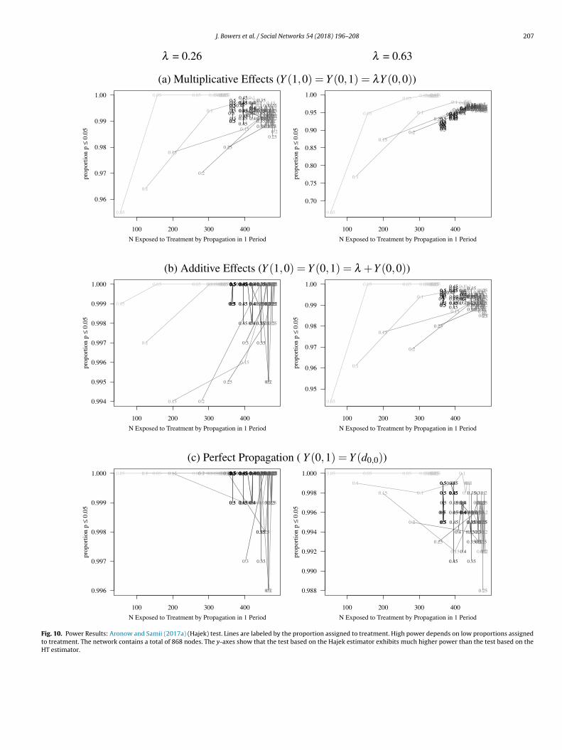
est approach to randomization of treatment assignment is simpleniform assignment without any blocking or use of informationbout the fixed network. To investigate this we study how power

9 Randomization distributions are simulated using a development version of theItools package for R (Bowers et al., 2014).10 It is notable that Aronow and Samii (2017a) present an alternative test, basedn a Hajek estimator that they show is more efficient than the HT estimator (with,owever, some bias). We present the results of this simulation using the Hajek esti-ator in Appendix A. We see that the Hajek estimator does exhibit higher power,

nd that we see the same patterns in terms of the proportion assigned to treatment.owever, we report the HT estimator in the main text, as some researchers may pre-

er to use the unbiased estimator, and, more practically speaking, the Hajek exhibitsuch high power that it is more difficult to see how power varies with the conditionsn the simulation study using the Hajek estimator, as compared to the HT estimator.

Ghana 2008 Voter Registration Fraud Experiment network. Vertices are registrationstations and yellow nodes are assigned to initial treatment.

depends on the correlation between m and Zi0 (i.e., the correlationbetween vertex degree and the initial treatment assignment) in thesimulation condition with the multiplicative effects and stochasticpropagation. The networks depicted in Fig. 5 represent examplesof treatment assignments biased in favor of high degree vertices(a) and low degree vertices (b). The degree-treatment correlationresults are given in Fig. 6. We can see in Fig. 6 that at each ˛value there is a strong positive relationship between the degree-treatment correlation and statistical power. This indicates that for

the Ghana network structure and the propagation/effects modelswe have specified, designs that bias treatment assignment towardshigher degree nodes would exhibit greater statistical power. This

204 J. Bowers et al. / Social Networks 54 (2018) 196–208

Fig. 6. When node degree is correlated with probability of treatment assignment, the power to detect indirect effects increases. Results are drawn from the simulationcondition with the multiplicative model of effects, and stochastic propagation of treatment.

100 200 300 400

0.5

0.6

0.7

0.8

0.9

1.0

Power to Reject the Sharp Null of No Effects

Prop

ortio

n p=

0.05

0.05

0.1

0.15

0.2

0.25 0.30.350.40.450.5

0.050.10.150.20.250.30.350.40.450.5

100 200 300 400

0.5

0.6

0.7

0.8

0.9

1.0

Power to Reject the Sharp Null of No Difference D01 vs D00

Prop

ortio

n p=

0.05

0.05

0.1

0.15

0.2 0.250.3 0.350.40.45

0.5

0.050.10.150.20.250.30.350.40.450.5

ue Isi

figta

N Exposed to Treatment by Propa gation in 1 Period

Fig. 7. Power with multiplicative effects model and tr

nding generalizes what we know about the use of prognostic back-round covariates to increase power in randomized experiments tohe situation where network degree can be thought of as a moder-tor of treatment effects.

N Exposed to Treatment by Propa gation in 1 Period

ng propagation model following Bowers et al. (2013).

The results from the model-testing methods of Bowers et al.(2013) in Figs. 7–9 differ in their implications from the results basedon estimation. First, the power in these tests is much higher overall.This makes some sense: we are assessing the ability of the test to

J. Bowers et al. / Social Networks 54 (2018) 196–208 205

100 200 300 400

0.70

0.75

0.80

0.85

0.90

0.95

1.00

Power to Reject the Sha rp Null of No Effects

N Exposed to Treatment by Propagation in 1 Period

Prop

ortio

n p

<=

0.0

5

0.05

0.1

0.15

0.2 0.25 0.30.350.40.450.5

0.050.10.150.20.250.30.350.40.450.5

100 200 300 400

0.70

0.75

0.80

0.85

0.90

0.95

1.00

Power to Reject the Sha rp Null of No Diffe rence D01 vs D00

N Exposed to Treatment by Propagation in 1 Period

Prop

ortio

n p

<=

0.0

5

0.05 0.1

0.150.2 0.25

0.30.350.40.45

0.5

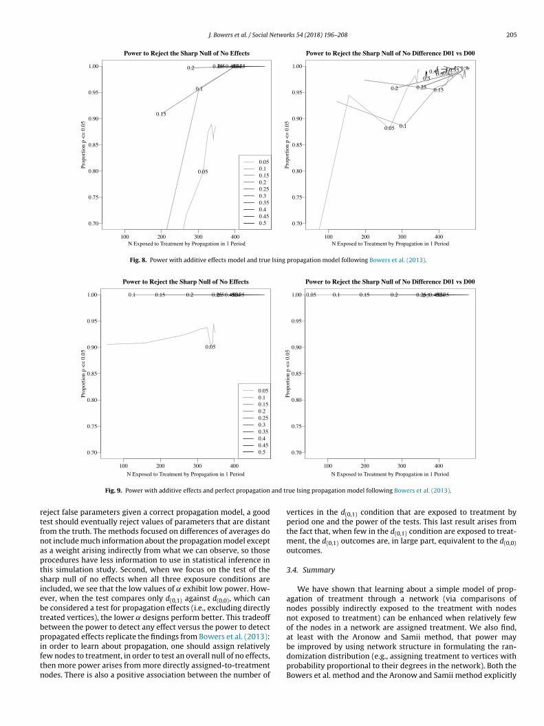
Fig. 8. Power with additive effects model and true Ising propagation model following Bowers et al. (2013).

100 200 300 400

0.70

0.75

0.80

0.85

0.90

0.95

1.00

Power to Reject the Sha rp Null of No Effects

Prop

ortio

n p

<=

0.0

5

0.05

0.1 0.15 0.2 0.25 0.30.350.40.450.5

0.050.10.150.20.250.30.350.40.450.5

100 200 300 400

0.70

0.75

0.80

0.85

0.90

0.95

1.00

Power to Reject the Sha rp Null of No Diffe rence D01 vs D00Pr

opor

tion

p <

= 0

.05

0.05 0.1 0.15 0.2 0.25 0.30.350.40.450.5

and tr

rtfnaptsiebtbpiftn

N Exposed to Treatment by Propa gation in 1 Period

Fig. 9. Power with additive effects and perfect propagation

eject false parameters given a correct propagation model, a goodest should eventually reject values of parameters that are distantrom the truth. The methods focused on differences of averages doot include much information about the propagation model excepts a weight arising indirectly from what we can observe, so thoserocedures have less information to use in statistical inference inhis simulation study. Second, when we focus on the test of theharp null of no effects when all three exposure conditions arencluded, we see that the low values of ̨ exhibit low power. How-ver, when the test compares only d(0,1) against d(0,0), which cane considered a test for propagation effects (i.e., excluding directlyreated vertices), the lower ̨ designs perform better. This tradeoffetween the power to detect any effect versus the power to detectropagated effects replicate the findings from Bowers et al. (2013):

n order to learn about propagation, one should assign relativelyew nodes to treatment, in order to test an overall null of no effects,hen more power arises from more directly assigned-to-treatmentodes. There is also a positive association between the number of

N Exposed to Treatment by Propa gation in 1 Period

ue Ising propagation model following Bowers et al. (2013).

vertices in the d(0,1) condition that are exposed to treatment byperiod one and the power of the tests. This last result arises fromthe fact that, when few in the d(0,1) condition are exposed to treat-ment, the d(0,1) outcomes are, in large part, equivalent to the d(0,0)outcomes.

3.4. Summary

We have shown that learning about a simple model of prop-agation of treatment through a network (via comparisons ofnodes possibly indirectly exposed to the treatment with nodesnot exposed to treatment) can be enhanced when relatively fewof the nodes in a network are assigned treatment. We also find,at least with the Aronow and Samii method, that power may

be improved by using network structure in formulating the ran-domization distribution (e.g., assigning treatment to vertices withprobability proportional to their degrees in the network). Both theBowers et al. method and the Aronow and Samii method explicitly

2 etwo

anblmhtitwtwotdifteriprae

waa2vodt

owifcncdivsnbsGttsfdmtn

06 J. Bowers et al. / Social N

ccount for the randomization distribution, and we are, as such,ot concerned about introducing bias into the methodology byiasing the randomization distribution. This would be a particu-

arly important method if the researcher hypothesized that theodel of effects varied with respect to network structure (e.g., a

ypothesis that higher degree vertices are more susceptible to thereatment). Since the randomization distribution is incorporatednto the methods we present, both approaches could be used toest hypotheses regarding effects that vary with respect to net-ork structure. More abstractly, our analysis acts an example for

hose desiring to evaluate their own models of propagation on net-orks and experimental designs before going into the field. Indeed,

ur findings that the power-maximizing proportion assigned toreatment falls well below 0.50, and power can be increased byisproportionately assigning treatment to higher degree nodes

s specific to the network dynamics that we artificially designedor this simulation study (i.e., the Ghana road network structure,he Ising model for treatment propagation, and our model(s) offfects). However, simulation studies such as the ones we haveun would assist the researcher in optimally designing the exper-ment given a network structure, and model(s) that characterizedropagation and treatment effects. We do not consider our findingsegarding the proportion assigned to treatment and disproportion-te assignment to highly connected nodes to apply universally toxperiments on networks.

We have not shown how Bowers et al. (2013) approach performshen an incorrect model is assessed. We did not do this because we

re focusing on design — and power analysis requires that we create truth against which to compare alternatives. Bowers et al. (2013,016) show that, in the analysis stage, hypothesis tests may haveery low or no power if the model being assessed has no bearingn the underlying mechanism, but we are not certain what kind ofesign advice would follow from such findings — merely increasinghe size of a fixed network may be impossible.

We have also not considered, for either Aronow and Samiir Bowers et al. methods, how design affects statistical powerhen there is uncertainty regarding the network structure. To

ncorporate uncertainty regarding the network, a stochastic modelor the network would need to be integrated into the analyti-al procedure(s) (e.g., Desmarais and Cranmer, 2012). Relatedly,etwork-based sampling methods (e.g., snowball sampling) areommonly used to study hard-to-reach populations (e.g., illicitrug users (Wang et al., 2007)). If researchers are introducing

nterventions in network-based samples, the effects of the inter-entions may include interference. There is an active literature intatistics and computer science that considers the ways in whichetwork quantities (e.g., prevalence of a behavior, degree distri-ution) can be accurately and efficiently estimated via networkampling designs (Handcock and Gile, 2010; Kurant et al., 2012;ile and Handcock, 2010). We have not thoroughly considered how

he tests studied in the current paper, and associated approacheso treatment assignment, would perform in the context of networkampling, but future work should consider the integration of testsor and estimates of interference effects with network sampling

esigns. Such consideration would involve the assessment of opti-al treatment assignment distributions (e.g., disproportionately

reating higher degree nodes) based on noisy information regardingetwork structure, gathered through a network sampling design.

rks 54 (2018) 196–208

4. Conclusion

We describe the challenges in experimental design that arisewhen the researcher is interested in studying the process ofpropagation on a network with the objective of drawing causalinference. The experimental designs that work most effectively inexperiments in which there is no interference are unlikely to bedirectly transferable to experimental research on propagation. Wereview two recently developed frameworks for statistical inferenceregarding interference in networks. One commonality we drawfrom these two frameworks is that theoretical analytic models ofpropagation play a key role in their application, which means thatsubstantive theory about the nature of treatment effects and net-work relations features more prominently in the statistical analysisof experimental data generated for the study of propagation thanin the classical, non-interference, experimental framework.

We present a simulation study to (1) illustrate how simulationcan be a useful guide in identifying design parameters for experi-mental studies of interference, and (2) study the properties of thetwo frameworks for statistical inference presented in the front endof the paper. Three findings from the simulation study are notable.First, statistical power depends upon design parameters and, forexample, the optimal proportion assigned to initial treatment maybe much lower than the conventionally applied 0.5.11 Second, therelationship between design parameters and power depends uponthe framework for statistical inference. Third, our results regardingthe positive relationship between the degree-treatment correla-tion and power indicates that randomization designs that take intoaccount graph topology are likely to exhibit substantial power gainsover uniform randomization designs. It is important to note, how-ever, that these findings are specific to our simulation setup, andmay not apply directly to other network experiments defined bydifferent networks, models of propagation, and/or models of treat-ment effects. Nevertheless, the results from the simulation studyunderscore the importance of considering design parameters forexperimental studies of propagation, as the standards of the clas-sical experimental framework are unlikely to apply. We encouragethe use of such simulation studies to guide the design of experi-ments on networks.

Our results suggest three fruitful directions for future research.First, as noted above, the literature on network dynamics offersseveral possibilities for specifying models of propagation on net-works. Researchers may not have strong a priori theory regardingthe functional form of the propagation model. This leads to thefirst future direction — considering whether the propagation modelcan be learned algorithmically, or analyzed though a nonparamet-ric framework. Second, although we focused on power to detectindirect and direct effects, we were studying multiple hypotheses(two in this case). Our work here has made us wonder whetherdesigns to maximize power against combined tests of those (andother) hypotheses might look different from designs which aimonly at maximizing power to detect propagation or overall effects.The third question regards the network through which interferenceoccurs. Future work should consider precisely how uncertaintyregarding the network structure can be incorporated into the meth-ods we present.

Appendix A.

See Fig. 10

11 This finding is supported by Baird et al. (2017)’s study of partial intereference,networks where the nodes are isolated into subsets. They show similar results inregards the tradeoffs between power to detect direct and peer-effects while focusingon a version of Aronow and Samii estimator tailored for their specific design.

J. Bowers et al. / Social Networks 54 (2018) 196–208 207

Fig. 10. Power Results: Aronow and Samii (2017a) (Hajek) test. Lines are labeled by the proportion assigned to treatment. High power depends on low proportions assignedto treatment. The network contains a total of 868 nodes. The y-axes show that the test based on the Hajek estimator exhibits much higher power than the test based on theHT estimator.

2 etwo

R

A

A

A

A

B

B

B

B

B

B

B

B

B

B

C

CC

C

CD

D

D

E

F

GG

G

H

H

H

H

H

H

H

I

Walker, D., Muchnik, L., 2014. Design of randomized experiments in networks?Proc. IEEE 102 (12), 1940–1951.

Wang, J., Falck, R.S., Li, L., Rahman, A., Carlson, R.G., 2007. Respondent-drivensampling in the recruitment of illicit stimulant drug users in a rural setting:findings and technical issues? Addict. Behav. 32 (5), 924–937.

08 J. Bowers et al. / Social N

eferences

nderson, R.M.E., 1982. Population Dynamics of Infectious Diseases: Theory andApplications. Chapman and Hall.

ral, S., Walker, D., 2011. Creating social contagion through viral product design: arandomized trial of peer influence in networks? Manag. Sci. 57 (9), 1623–1639.

ronow, P.M., Samii, C., 2017a. Estimating average causal effects under generalinterference, with application to a social network experiment. Ann. Appl. Stat.

ronow, P.M., Samii, C., 2017b. Estimating Spatial Effects (UnpublishedManuscript).

aird, S., Bohren, J.A., McIntosh, C., Ozler, B., 2017. Optimal design of experimentsin the presence of interference. Rev. Econ. Stat.

apna, R., Umyarov, A., 2015. Do your online friends make you pay? A randomizedfield experiment on peer influence in online social networks. Manag. Sci. 61(8), 1902–1920.

ass, Frank, M., Krishnan, T.V., Jain, D.C., 1994. Why the bass model fits withoutdecision variables. Market. Sci. 13 (3), 204–223.

asse, G.W., Airoldi, E.M., 2015. Optimal Design of Experiments in the Presence ofNetwork-Correlated Outcomes. arXiv:1507.00803.

iswas, S., Sen, P., 2009. Model of binary opinion dynamics: coarsening and effectof disorder. Phys. Rev. E 80 (2), 027101.

ond, R.M., Fariss, C.J., Jones, J.J., Kramer, A.D., Marlow, C., Settle, J.E., Fowler, J.H.,2012. A 61-million-person experiment in social influence and politicalmobilization? Nature 489 (7415), 295–298.

owers, J., Fredrickson, M., Hansen, B., 2014. RItools: Randomization InferenceTools. R Package Version 0., pp. 1–12.

owers, J., Fredrickson, M., Panagopoulos, C., 2013. Reasoning about interferencebetween units: a general framework? Polit. Anal. 21 (1), 97–124.

owers, J., Fredrickson, M.M., Aronow, P.M., 2016. Research note: a more powerfultest statistic for reasoning about interference between units. Polit. Anal.,mpw018.

utler, D.M., Nickerson, D.W., et al., 2011. Can learning constituency opinion affecthow legislators vote? Results from a field experiment. Q. J. Polit. Sci. 6 (1),55–83.

hen, J., Humphreys, M., Modi, V., 2010. Technology Diffusion and Social Networks:Evidence From a Field Experiment in Uganda (Unpublished Manuscript).

lifford, P.A.W.S., 1973. A model for spatial conflict. Biometrika 60, 581–588.oppock, A., 2014. Information spillovers: another look at experimental estimates

of legislator responsiveness? J. Exp. Polit. Sci. 1 (02), 159–169.oppock, A., 2016. Information spillovers: another look at experimental estimates

of legislator responsiveness corrigendum? J. Exp. Polit. Sci. 3 (2), 206–208.ox, D.R., 1958. The Planning of Experiments. John Wiley.aley, D.J., Gani, J., 2005. Epidemic Modeling: An Introduction. Cambridge

University Press, NY.esmarais, B.A., Cranmer, S.J., 2012. Statistical inference for valued-edge networks:

the generalized exponential random graph model. PLoS ONE 7 (1), e30136.urrett, Richard, Kesten, H., 1991. Random Walks, Brownian Motion, and

Interacting Particle Systems. Springer.ckles, D., Karrer, B., Ugander, J., 2017. Design and analysis of experiments in

networks: reducing bias from interference. J. Causal Inference 5 (1).ortunato, S., 2005. The sznajd consensus model with continuous opinions? Int. J.

Mod. Phys. C 16 (01), 17–24.allavotti, G., 1999. Statistical Mechanics: A Short Treatise. New York, Springer.erber, A.S., Green, D.P., 2012. Field Experiments: Design, Analysis, and

Interpretation. WW Norton.ile, K.J., Handcock, M.S., 2010. Respondent-driven sampling: an assessment of

current methodology? Sociol. Methodol. 40 (1), 285–327.andcock, M.S., Gile, K.J., 2010. Modeling social networks from sampled data. Ann.

Appl. Stat. 4 (1), 5.ethcote, H.W., 2000. The mathematics of infectious diseases. Soc. Ind. Appl. Math.

42, 599–653.irano, K., Hahn, J., 2010. Design of randomized experiments to measure social

interaction effects? Econ. Lett. 106 (1), 51–53.olland, P.W., 1986. Statistics and causal inference? J. Am. Stat. Assoc. 81 (396),

945–960.opfield, J., 1982. Neural networks and physical systems with emergent collective

computational abilities? Proc. Natl. Acad. Sci. 79 (8), 2554–2558.orvitz, D.G., Thompson, D.J., 1952. A generalization of sampling without

replacement from a finite universe? J. Am. Stat. Assoc. 47 (260), 663–685.

udgens, M., Halloran, M., 2008. Toward causal inference with interference? J. Am.

Stat. Assoc. 103 (482), 832–842.chino, N., Schündeln, M., 2012. Deterring or displacing electoral irregularities?

Spillover effects of observers in a randomized field experiment in Ghana. J.Polit. 74, 292–307.

rks 54 (2018) 196–208

Kermack, W.O., McKendrick, A.G., 1927. A contribution to the mathematical theoryof epidemics. Math. Phys. Eng. Sci. 115 (772), 700.

Kingdon, J.W., 1989. Congressman’s Voting Decisions. Ann Arbor, MI. University ofMichigan Press.

Kurant, M., Gjoka, M., Wang, Y., Almquist, Z.W., Butts, C.T., Markopoulou, A., 2012.Coarse-grained topology estimation via graph sampling. In: Proceedings of the2012 ACM Workshop on Workshop on Online Social Networks, ACM, pp.25–30.

Lenk, P.J., Rao, A., 1990. New models from old: forecasting product adoption byhierarchical Bayes procedure? Market. Sci. 9 (1), 42–53.

Liggett, T.M., 1997. Stochastic models of interacting systems? Ann. Probab. 25 (1),1–2.

Lyons, R., 2011. The spread of evidence-poor medicine via flawed social-networkanalysis. Stat. Polit. Policy 2 (1).

Miguel, E., Kremer, M., 2004. Worms: identifying impacts on education and healthin the presence of treatment externalities? Econometrica 72 (1), 159–217.

Neyman, J., 1923 [1990. On the application of probability theory to agriculturalexperiments. Essay on principles. Section 9 (1923). Stat. Sci. 5, 463–480,Reprint. Transl. by Dabrowska and Speed).

Nickerson, D., 2008. Is voting contagious? Evidence from two field experiments.Am. Polit. Sci. Rev. 102 (01), 49–57.

Nickerson, D., 2011. Social networks and political context. In: CambridgeHandbook of Experimental Political Science., pp. 273.

Ostrovsky, M., Schwarz, M., 2011. Reserve prices in internet advertising auctions: afield experiment. In: Proceedings of the 12th ACM conference on Electroniccommerce, EC’11, New York, NY, USA. ACM, pp. 59–60.

Rubin, D.B., 1980. Randomization analysis of experimental data: the fisherrandomization test comment? J. Am. Stat. Assoc. 75 (371), 591–593.

Scholz, F.W., Stephens, M.A., 1987. K-sample anderson-darling tests? J. Am. Stat.Assoc. 82 (399), 918–924.

Shalizi, C.R., Thomas, A.C., 2011. Homophily and contagion are genericallyconfounded in observational social network studies? Sociol. Methods Res. 40(2), 211–239.

Sinclair, B., 2011. Design and analysis of experiments in multilevel populations. In:Cambridge Handbook of Experimental Political Science. Cambridge UniversityPress, pp. 906.

Sinclair, B., McConnell, M., Green, D.P., 2012. Detecting spillover effects: design andanalysis of multilevel experiments? Am. J. Polit. Sci. 56 (4), 1055–1069.

Sobel, M., 2006. What do randomized studies of housing mobility demonstrate? J.Am. Stat. Assoc. 101 (476), 1398–1407.

Sousa, A., Yu-Song, T., Ausloos, M., 2008. Effects of agents’ mobility on opinionspreading in sznajd model? Eur. Phys. J. B-Condens. Matter Complex Syst. 66(1), 115–124.

Tchetgen, E., VanderWeele, T., 2010. On causal inference in the presence ofinterference. Stat. Methods Med. Res.

Toulis, P., Kao, E., 2013. Estimation of causal peer influence effects. Proceedings ofthe 30th International Conference on Machine Learning, ICML’13.

VanderWeele, T., 2008. Ignorability and stability assumptions in neighborhoodeffects research? Stat. Med. 27 (11), 1934–1943.

VanderWeele, T., 2010. Direct and indirect effects for neighborhood-basedclustered and longitudinal data. Sociol. Methods Res. 38 (4), 515.

VanderWeele, T., Tchetgen, E., 2011. Bounding the infectiousness effect in vaccinetrials? Epidemiology 22 (5), 686–693.

VanderWeele, T., Tchetgen, E., Halloran, M., 2011. Components of the indirecteffect in vaccine trials: identification of contagion and infectiousness effects.COBRA Preprint Series, 85.

VanderWeele, T., Tchetgen Tchetgen, E., 2011. Effect partitioning underinterference in two-stage randomized vaccine trials. Stat. Probab. Lett. 81 (7),861–869.

VanderWeele, T., Vandenbroucke, J., Tchetgen Tchetgen, E., Robins, J., 2012. Amapping between interactions and interference: implications for vaccinetrials. Epidemiology 23 (2), 285.

Vazquez, F., Krapivsky, P.L., Redner, S., 2003. Constrained opinion dynamics:freezing and slow evolution. J. Phys. A: Math. Gen. 36 (3), L61.