Models of the very early universe with

multiple scalar fields

Mathew Robinson

Submitted for the degree of Doctor of Philosophy

School of Mathematics and Statistics, University of Sheffield

September 2015

Supervisor: Prof. Carsten van de Bruck

Abstract

There is a reasonable amount of observational evidence that sug-

gests space was expanding exponentially in the very early universe —

an expansion that has become known as inflation. The mechanism by

which this happens remains up for debate, however, and this thesis

looks at a number of potential scenarios using multiple scalar fields

to drive the expansion. There are two studies that look at how ad-

ditional couplings either between the fields themselves or to gravity

can influence the observable consequences of inflation on the Cosmic

Microwave Background and one which tries to extend a gravitational

coupling to explain the current expansionary epoch caused by dark

energy. The importance of reheating in such scenarios is also inves-

tigated. In the case of a non-canonical kinetic coupling, an approxi-

mation is used to show how the curvature perturbation can evolve on

super-horizon scales to a much improved accuracy over previous work.

The gravitational coupling results in a vast increase in the amplitude

of the curvature power spectrum via the non-adiabatic pressure per-

turbation and, finally, the attempts to link this to dark energy are

demonstrated to be much more difficult than one might initially as-

sume.

iv

v

Preface

This thesis is submitted in partial fulfillment of the requirements for a degree

of Doctor of Philosophy in Mathematics. The project has been supervised

by Prof. Carsten van de Bruck and the contents of this thesis are largely the

work original work of the Author.

• Chapter 1 contains a general introduction to cosmology and inflation

along with summary sections on reheating, observational quantities and

potential extensions to the basic model.

• Chapter 2 takes the general ideas a bit further and introduces pertur-

bations and the effects of them on observable quantities.

• Chapter 3 is based on the published work in the Journal of Cosmology

and Astroparticle Physics in April 2014 with Carsten van de Bruck [1].

All analytical and numerical calculations along with the production of

figures was done by the Author unless explicitly stated and referenced

otherwise within the text.

• Chapter 4 is based on the published work in Physical Review D in

June 2015 [2] in collaboration with Carsten van de Bruck and Adam

Christopherson. All numerical work, analytical work and figures were

again produced solely by the Author.

• Chapter 5 gives conclusions based on the preceding two chapters along

with an as yet unpublished extension that has been done in collabora-

tion with Carsten van de Bruck and Konstantinos Dimopoulos. After

a short review of previous work, clearly referenced, all subsequent nu-

merical work is the sole work of the Author.

vi

vii

Acknowledgements

Firstly, I would like to thank Carsten for his support throughout these four

years in Sheffield. Despite the pressures of various departmental duties, he

always managed to find the time to help whenever it was needed and for as

long as it was needed — I could not have wished for a more attentive and

friendly supervisor than him. I’d also like to thank Adam and Kostas for

their help and ideas in our collaborations.

I, of course, must also thank Keri for her unerring support in both mov-

ing to Sheffield in the first place, and letting me stay up late once in a while

to ‘work’. Then there is my family, without whom I’d never have become

such a questioning, argumentative person — qualities that inevitably set me

on my way into this most fundamental of sciences.

Lastly, I am endlessly grateful for the Peak District National Park — and

the many hundreds of hours of relaxing solitude and time to think that it

allowed me — without which my sanity may well have been lost long ago.

viii

ix

“It is a great adventure to contemplate the universe, beyond man, to

contemplate what it would be like without man, as it was in a great

part of its long history and as it is in a great majority of places.

When this objective view is finally attained, and the mystery and

majesty of matter are fully appreciated, to then turn the objective eye

back on man viewed as matter, to view life as part of this universal

mystery of greatest depth, is to sense an experience which is very

rare, and very exciting. It usually ends in laughter and a delight in

the futility of trying to understand what this atom in the universe

is, this thing — atoms with curiosity — that looks at itself and

wonders why it wonders. Well, these scientific views end in awe and

mystery, lost at the edge in uncertainty, but they appear to be so deep

and so impressive that the theory that it is all arranged as a stage

for God to watch man’s struggle for good and evil seems inadequate.”

- R. Feynman — The Meaning of It All: Thoughts of a Citizen-

Scientist

x

xi

Contents

Abstract iv

Preface vi

Acknowledgements viii

List of Figures xvi

List of Tables xxii

1 Introduction 1

1.1 Cosmology . . . . . . . . . . . . . . . . . . . . . . . . . . . . . 1

1.2 The Cosmic Microwave Background . . . . . . . . . . . . . . . 4

1.3 Cosmological dynamics . . . . . . . . . . . . . . . . . . . . . . 4

1.4 Inflation . . . . . . . . . . . . . . . . . . . . . . . . . . . . . . 7

1.4.1 Types of inflation: large, small or something inbetween? 10

1.4.2 efolds . . . . . . . . . . . . . . . . . . . . . . . . . . . 11

1.5 Reheating . . . . . . . . . . . . . . . . . . . . . . . . . . . . . 14

1.5.1 Perturbative reheating . . . . . . . . . . . . . . . . . . 15

1.5.2 Preheating . . . . . . . . . . . . . . . . . . . . . . . . . 17

1.6 Observational Quantities . . . . . . . . . . . . . . . . . . . . . 20

1.7 Inflationary Extensions . . . . . . . . . . . . . . . . . . . . . . 24

1.7.1 Multiple Fields . . . . . . . . . . . . . . . . . . . . . . 24

1.7.2 The Curvaton Scenario . . . . . . . . . . . . . . . . . . 28

1.7.3 Further Extensions? . . . . . . . . . . . . . . . . . . . 28

2 Perturbations 32

xii

2.1 Gauges . . . . . . . . . . . . . . . . . . . . . . . . . . . . . . . 34

2.2 Other perturbed quantities . . . . . . . . . . . . . . . . . . . . 38

2.3 Returning to the observables . . . . . . . . . . . . . . . . . . . 42

2.4 The Curvaton . . . . . . . . . . . . . . . . . . . . . . . . . . . 45

3 Second order slow-roll with

non-canonical kinetic terms 55

3.1 Non-canonical kinetic terms . . . . . . . . . . . . . . . . . . . 57

3.2 Extending the analytics . . . . . . . . . . . . . . . . . . . . . 58

3.2.1 Slow-Roll . . . . . . . . . . . . . . . . . . . . . . . . . 61

3.2.2 The evolution of the scale factor . . . . . . . . . . . . . 63

3.2.3 Horizon Crossing . . . . . . . . . . . . . . . . . . . . . 66

3.3 Evolution on super-Hubble scales . . . . . . . . . . . . . . . . 74

3.4 Numerical setup, initial conditions and potentials . . . . . . . 76

3.5 Numerical results . . . . . . . . . . . . . . . . . . . . . . . . . 84

3.5.1 Double Inflation . . . . . . . . . . . . . . . . . . . . . . 85

3.5.2 Quartic Potential . . . . . . . . . . . . . . . . . . . . . 88

3.5.3 Hybrid Inflation . . . . . . . . . . . . . . . . . . . . . . 92

3.5.4 Product potential . . . . . . . . . . . . . . . . . . . . . 92

3.5.5 b(φ) = βφ2 example - double quadratic potential . . . . 93

3.6 Conclusions . . . . . . . . . . . . . . . . . . . . . . . . . . . . 96

4 Stabilising the Planck mass after inflation 99

4.1 Non-minimally coupled curvaton . . . . . . . . . . . . . . . . . 100

4.2 Numerics . . . . . . . . . . . . . . . . . . . . . . . . . . . . . 111

4.3 Results . . . . . . . . . . . . . . . . . . . . . . . . . . . . . . . 117

4.3.1 The case: σmin = σini . . . . . . . . . . . . . . . . . . . 117

4.3.2 The case: σmin 6= σini . . . . . . . . . . . . . . . . . . . 121

xiii

4.3.3 The case: σmin = 0 . . . . . . . . . . . . . . . . . . . . 123

4.4 Some concluding remarks . . . . . . . . . . . . . . . . . . . . . 124

5 Conclusions and a future direction 127

5.1 A Gauss-Bonnet encore . . . . . . . . . . . . . . . . . . . . . . 130

5.1.1 The equations of motion . . . . . . . . . . . . . . . . . 131

5.1.2 Reheating in Gauss-Bonnet inflation . . . . . . . . . . 132

5.1.3 Observational constraints . . . . . . . . . . . . . . . . . 133

5.1.4 A few example models . . . . . . . . . . . . . . . . . . 134

A Appendix 141

A.1 Time dependence of the slow-roll parameters . . . . . . . . . . 141

A.2 Evaluating f(x) and g(x) . . . . . . . . . . . . . . . . . . . . . 143

A.2.1 f(x) — the first order function . . . . . . . . . . . . . 143

A.2.2 g(x) — the second order function . . . . . . . . . . . . 144

Bibliography 147

xiv

xv

List of Figures

1 A simple demonstration of how the total perturbation in φ

and χ can instead be decomposed into analogous δσ and δs

components. . . . . . . . . . . . . . . . . . . . . . . . . . . . . 26

2 Taken from [73]. The red lines are for mσ mφ, the blue

lines show mσ = mφ/2 and the green lines show the inflating

curvaton scenario — in which a second period of inflation is

driven by the curvaton before it decays. . . . . . . . . . . . . . 52

3 Inflationary trajectories. The top left panel shows the double

quadratic potential with b(φ) = 0 and the top right shows it

with b(φ) = φ. The middle row shows the quartic potential

on the left and the hybrid evolution on the right. Finally the

bottom row shows the product potential trajectory on the left

and, on the right, the second order non-canonical term case of

double quadratic inflation — so b(φ) = φ2. . . . . . . . . . . . 84

4 Canonical double inflation with mχ/mφ = 7. The left graph

shows the evolution of the slow roll parameters for canonical

double inflation. The right graph shows the resulting power

spectra with the solid black lines representing the numerical

results, the dotted lines representing the first order results and

the dashed lines representing the second order results. . . . . . 86

xvi

5 Canonical double inflation with mχ/mφ = 10. The left graph

shows the evolution of the slow roll parameters. The right

graph shows the resulting power spectra with the solid black

lines representing the numerical results, the dotted lines repre-

senting the first order results and the dashed lines representing

the second order results. . . . . . . . . . . . . . . . . . . . . . 86

6 Non-canonical double inflation with mχ/mφ = 7. The left

graph shows the evolution of the slow roll parameters - with

ξ1 dominating. The right graph shows the resulting power

spectra with the solid black lines representing the numerical

results, the dotted lines representing the first order results and

the dashed lines representing the second order results. . . . . . 89

7 Non-canonical double inflation with mχ/mφ = 1/3. The left

graph shows the evolution of the slow roll parameters - now

with both ξ1 and ηss dominating. The right graph shows the

resulting power spectra with the solid black lines representing

the numerical results, the dotted lines representing the first or-

der results and the dashed lines representing the second order

results. . . . . . . . . . . . . . . . . . . . . . . . . . . . . . . . 89

8 Quartic potential. The left graph shows the evolution of the

slow roll parameters. The right graph shows the resulting

power spectra with the solid black lines representing the nu-

merical results, the dotted lines representing the first order

results and the dashed lines representing the second order re-

sults. . . . . . . . . . . . . . . . . . . . . . . . . . . . . . . . . 90

xvii

9 Canonical hybrid inflation. The left graph shows the evolution

of the slow roll parameters — which all remain relatively small.

The right graph shows the resulting power spectra with the

solid black lines representing the numerical results, the dotted

lines representing the first order results and the dashed lines

representing the second order results. . . . . . . . . . . . . . . 91

10 Non-canonical hybrid inflation with β = 10. The left graph

shows the evolution of the slow roll parameters — which,

again, all remain relatively small. The right graph shows the

resulting power spectra with the solid black lines representing

the numerical results, the dotted lines representing the first or-

der results and the dashed lines representing the second order

results. . . . . . . . . . . . . . . . . . . . . . . . . . . . . . . . 91

11 Product potential. The left graph shows the evolution of the

slow roll parameters. The right graph shows the resulting

power spectra with the solid black lines representing the nu-

merical results, the dotted lines representing the first order

results and the dashed lines representing the second order re-

sults. . . . . . . . . . . . . . . . . . . . . . . . . . . . . . . . . 94

12 Non-canonical product potential, with b(φ) = 0.1φ. The left

graph shows the evolution of the slow roll parameters. The

right graph shows the resulting power spectra with the solid

black lines representing the numerical results, the dotted lines

representing the first order results and the dashed lines repre-

senting the second order results. . . . . . . . . . . . . . . . . . 94

xviii

13 Double quadratic inflation with a higher order coupling term

(b(φ) = φ2). Here, the left graph power spectra with the solid

black lines representing the numerical results, the dotted lines

representing the first order results and the dashed lines repre-

senting the second order results — without the new second

order non-canonical terms (ξ2) included. The right hand graph

shows exactly the same, but with all terms included. . . . . . 95

14 Top: The evolution of the relative energy density in each

species, Ωi for both the α = 0 and α = −0.005 cases, which

overlap throughout. Bottom left: The background evolution

of σ for both α values and for σmin = σini = 0.1. Bottom right:

The evolution of the effective Planck mass for α = −0.005

when σmin = σini = 0.1 — where MP is defined as√f(σ) and

normalised to 1 at its final value. . . . . . . . . . . . . . . . . 118

15 The power spectrum of the curvature perturbation (left) for

both α = 0 and α = −0.005 cases and the associated δPnad

(right). . . . . . . . . . . . . . . . . . . . . . . . . . . . . . . . 118

16 The amplitude of the power spectrum as a function of α nor-

malised to the α = 0 power spectrum: Pζ(α)/Pζ(0). . . . . . . 120

17 Amplitude of the power spectrum Pζ as a function of α for

three different values of σend = 0.1, 0.2, 0.3 . . . . . . . . . . . 121

18 Left: The power spectra for varying α with σini = 0.3 and

σmin = 0.1 (red) in comparison to the case of σini = σmin = 0.1

(blue). Right: The background trajectories for σ for each of

these cases. . . . . . . . . . . . . . . . . . . . . . . . . . . . . 123

xix

19 The evolution of the ratios of the of the components of the

universe, Ωφ,σ,γ, is shown on the left — and a scaled version

of the actual energy densities, ρφ,σ,γ to show the qualitative

behaviour on the right. Both are given for the last few efolds

of inflation and subsequent evolution. . . . . . . . . . . . . . . 136

20 The evolution of Ωφ and Ωγ for two choices of α and Γφ,

showing the evolution throughout inflation and in the sub-

sequent expansion. The left hand plot uses Γφ = 0.001 and

α = 0.00001 whilst the right hand plot uses Γφ = 0.001 and

α = 0.000001. . . . . . . . . . . . . . . . . . . . . . . . . . . . 137

21 The final values of Ωφ for various choices of α and Γφ roughly

30 efolds after the end of inflation — showing the relation-

ship between the two variables. The decay rates are all scaled

relative to the mass of the inflaton, ie. the label ’Γφ = 0.1’

represents ’Γφ = 0.1mφ . . . . . . . . . . . . . . . . . . . . . . 138

22 The evolution of Ωφ, Ωγ and Ωm using the same values of α

and Γφ as that used in the right hand side of Figure 20 —

along with the inclusion of Γmφ = 10−8 . . . . . . . . . . . . . . 139

xx

xxi

List of Tables

1 A table clarifying our notation for the subscripts denoting var-

ious stages in the evolution of σ. . . . . . . . . . . . . . . . . . 109

xxii

xxiii

1 Introduction

1.1 Cosmology

For many thousands of years, humans have gazed up at the night sky and had

an interest in where we came from, what’s out there and how any of it came

into existence. For a long time, this was the realm of religion and mythology

but in the last couple of millennia the scientific method has increasingly

come to the forefront of explaining the cosmos — and our place within it.

Since the turn of the 20th century the rate of understanding has increased

dramatically — with the advent of special relativity [3], general relativity [4]

and quantum mechanics [6] allowing modern cosmology to flourish. It was

noticed by Einstein that his field equations naturally led to a universe which

was not dynamically stable, preferring instead to either expand or contract.

This was seen as a problem with the framework of general relativity and led to

the introduction of a non-zero constant, the so called ‘cosmological constant’,

in order to allow for the presumed steady state nature of the universe at the

time. This was not, however, the full story, as it was soon postulated, by

Friedmann, that a dynamic universe was also an attractive solution to the

field equations [5]. In 1929, it was realised by Edwin Hubble that the universe

was, in fact, expanding [7] — he revealed that almost every galaxy in the

visible universe was receding from our reference point within the Milky Way.

Not only this, but also that the further away a galaxy was, the faster it was

moving away; a trend which subsequently became known as Hubble’s Law,

v = Hd, (1.1)

in which v is the velocity of recession, d is the distance and H is the Hub-

ble constant (which, later, becomes the H(t) as we realise the time depen-

1

dence of this parameter). The current value of H is found to be H0 =

(67 ± 1.2)kms−1Mpc−1 [10]. This discovery led physicists to eventually as-

sume that the cosmological constant was zero all along and that the only

explanation for such an observation was that the universe did in fact evolve

in time and was, more precisely, expanding. The expansion of the universe

was all but confirmed by Penzias and Wilson in the 1960’s with the discovery

of the cosmic microwave background radiation (CMB) [11] which has, itself,

ushered in the era of precision cosmology which continues to this day. Finally,

in the late 20th century the most recent change to the prevailing cosmolog-

ical paradigm occurred, as it became clear that not only was the universe

expanding, the expansion was once again accelerating. This late-time expan-

sion, caused by some as yet mysterious dark energy, can interchangeably be

labeled as the cosmological constant disregarded decades earlier.

If the universe is expanding, extrapolating back naturally leads to the

idea that at some point in the past it was much smaller and possibly even

came from a single point — from this, the big bang theory was born. This is

not, however, the full story, as there remained three significant problems with

this theory which can be solved by the inclusion of a period of exponential

expansion in the early universe, inflation [12, 13]. The problems and solutions

are as follows:

1. The Horizon Problem: the near-homogenous, isotropic nature of

the CMB defies the basic principles of causality in the standard big

bang scenario. How could two regions of space, so far apart that it

is impossible for them to have ever been in contact, have the same

properties — such as temperature and structure — in the present day?

A period of inflation overcomes this problem as it allows that before the

exponential expansion these two regions could have been much closer

2

together and come to such an equilibrium early on.

2. The Flatness Problem: the universe has been observed to be very

nearly, if not exactly, spatially flat — with a density parameter (defined

by Ω = ρtot/ρcrit, where ρcrit is the critical density required for a Eu-

clidean universe), Ω = 1.0005± .07 [14]. This would require significant

fine tuning to occur as a result of the standard big bang model as any

deviation from flatness (Ω = 1) throughout the history of the universe

would increase exponentially in time. This is solved by inflation as

any such deviations are quickly stretched out in the early universe —

avoiding this instance of fine-tuning completely.

3. The Magnetic Monopole Problem: it is predicted by numerous

particle theories, beyond the standard model, that magnetic monopoles

should exist in nature. The fact that they are yet to be observed

hints at another problem with standard cosmology. As before, inflation

solves this in a simple and intuitive way. If the monopoles are created

early enough, before inflation has ended, the density is diluted by the

subsequent expansion to such an extent that we could never expect to

spot them in the observable universe.

The fact that inflation solves so many of these problems in a very natural

way has led to it being the leading theory of the early stages of the universe’s

expansion. Following this period of inflation, it is believed that a period of

reheating occurred which resulted in a radiation dominated epoch followed

by matter domination, baryogenesis and nucleosynthesis. From this point,

the evolution follows that predicted by the standard big bang model once

more.

3

1.2 The Cosmic Microwave Background

The Cosmic Microwave Background (CMB) is nothing more than an image

of the universe imprinted just after the recombination epoch in the early uni-

verse [15, 16, 17]. This occurred after ∼ 377000 years, when the universe had

expanded and cooled sufficiently to allow protons and electrons to be bound

to form neutral Hydrogen. Before this, the mean free path of the photons was

so short, due to Thomson scattering with the free electrons, as to render the

universe effectively opaque. As Hydrogen atoms formed and the radiation

decoupled from matter it was then able to travel relatively freely throughout

the subsequent evolution of the universe. Over that remaining time, the ex-

pansion of the universe has cooled the radiation of the CMB to have a mean

temperature of just 2.72548 ± 0.00057 K — but, fortunately, the spectrum

is not quite a perfect black body spectrum — with interesting features that

we can directly relate back to the conditions found during the formation of

the radiation. Since the discovery of the CMB, numerous experiments have

been devised in order to ascertain as much information as possible from these

discrepancies with COBE (1989) [18, 19], WMAP (2001) [20, 21, 22] and now

Planck (2009) [10, 23, 24, 25, 26, 27] continually improving on the resolution

of the observations.

1.3 Cosmological dynamics

Before going any further, it is important to make clear a few definitions that

will be used throughout this thesis. In terms of derivatives, an overdot (X)

is used to indicate a derivative with respect to cosmic time, t, and – unless

otherwise stated – a dash (X ′) is used to denote derivatives with respect to

efold number, N , which shall itself be defined shortly. Beginning from the

4

basics of time and space we can define a line element, describing the four

dimensional distance between two points, as

ds2 =∑µν

gµνdxµdxν , (1.2)

where µ and ν take values from 0−3, xµ,ν represent the dimensions of space-

time and gµν is the metric. Following convention, we allow x0 to signify time

whilst xi,j, i, j = 1, 2, 3 denotes the spatial components. The most general

metric, appropriate to standard cosmology — where on large scales, homo-

geneity and isotropy are assumed — is the Friedmann-Lemaitre-Robertson-

Walker (FLRW) metric,

ds2 = −dt2 + a2(t)

(dr2

1− κr2+ r2(dθ2 + sin2(θ)dφ2)

), (1.3)

where a is defined as the scale factor, κ = −1, 0,+1 gives an open, flat or

closed universe respectively. The Hubble parameter can be defined as follows:

H =a

a. (1.4)

From here the space-time dynamics evolve according to the Einstein equa-

tions,

Gµν + Λgµν = Rµν −1

2Rgµν + Λgµν = 8πGTµν , (1.5)

where Tµν is the energy momentum tensor that we shall come to shortly and

Rµν is the Ricci tensor defined by,

Rµν = Γανµ,α − Γααµ,ν + ΓααβΓβνµ − ΓανβΓβαµ. (1.6)

The dynamics can be studied using the non-vanishing components of the

Einstein tensor,

G00 = 3(H2 +

κ

a2

)and Gij =

(H2 + 2

a

a+κ

a2

), (1.7)

5

where, for a flat universe, κ = 0, and the FLRW metric reduces to

ds2 = −dt2 + a2(t)γij(xk)dxidxj, (1.8)

where γij still represents the metric of a 3 dimensional sphere. The energy-

momentum tensor, Tµν , is defined for a perfect fluid as follows:

T µν =

−ρ 0 0 0

0 p 0 0

0 0 p 0

0 0 0 p

(1.9)

in which we have introduced both the energy density, ρ, and pressure, p,

which are both solely functions of time. Rµν and R are the Ricci tensor and

scalar respectively, calculated from the metric in the usual way [28].

The Einstein equations then reduce to the Friedmann equations (assum-

ing a vanishing cosmological constant) as

H2 =8πG

3ρ (1.10)

anda

a= −8πG

6(ρ+ 3p) (1.11)

along with the matter conservation equation coming from ∇µTµν = 0,

ρ+ 3H(ρ+ p) = 0.. (1.12)

These can be used alongside an equation of state for the matter to form

a closed set of equations for a, ρ and p. As such, we set the equation of state

as

p = ωρ. (1.13)

Now, for an accelerated expansion (inflation) to occur, it is necessary that

a > 0. For this to happen, it can be seen from Eq. (1.11) that ρ+ 3p < 0 or,

6

more usefully, that p < −ρ3. In order to simplify this further, it is often taken

that p = −ρ, dropping the factor of 3, in which case we have an inflationary

period known as the de Sitter phase which corresponds to ω = −1 in the

equation of state. Similarly, we know that during a radiation dominated

epoch ω = 1/3 and during a pressureless matter phase ω = 0.

During each of these stages of evolution the scale factor evolves in a

different way. By solving Eq. (1.11) and Eq. (1.12) it is possible to show

that

ρ ∝ a−3(1+ω) and a ∝ t2/3(1+ω), (1.14)

such that for an inflationary era, ρ = const, for a radiation dominated uni-

verse

ργ ∝1

a4and a ∝ t1/2, (1.15)

and for a matter dominated universe

ρm ∝1

a3and a ∝ t2/3. (1.16)

1.4 Inflation

Coming back to inflation, mentioned a little earlier, it is now necessary to take

a look in a little more detail and formalise what is achieved by having a > 0

and how this comes about. To begin with, only focusing on the background

and ignoring the presence of any spacially dependent perturbations, inflation

can be driven by a scalar field, φ(t), known as the inflaton — the action of

which is given by

Sφ = −∫d4x√−g(∂µφ∂

µφ

2+ V (φ)

)(1.17)

7

where g is the determinant of the metric, ∂µφ∂µφ

2is known as the kinetic term

and V (φ) is some potential that depends on the inflaton. By varying the

action with respect to the scalar field, it is relatively straightforward to show

that the inflaton is governed by the following equation of motion,

φ+ 3Hφ+ Vφ = 0 (1.18)

where Vφ denotes the derivative of V with respect to φ. This is to say that,

given an arbitrary potential and initial value of φ away from its minimum

— the field will roll down the potential towards said minimum. It is this

that drives inflation. There is, however, an additional term in Eq. (1.18)

which also plays an important role — the friction term, 3Hφ. We know

from the definition of H that this is related to the scale factor, a, and so

depends on the expansion of the universe. The complete action, S consists

of both the part relating to the scalar field, Sφ, and the Einstein-Hilbert

action, SH = 12

∫(R− 2Λ)

√−gd4x, such that

S =1

8πGSH + Sφ. (1.19)

Similarly to how we found the equation of motion, we can instead vary the

total action with respect to the metric itself, gµν , to recover not only the

Einstein equations (Eq. (1.5)) but also the form of the energy-momentum

tensor in terms of the scalar field — finding

Tµν = − 2√−g

δSφδgµν

= ∂µφ∂νφ−gµν2∂αφ∂

αφ− gµνV (φ). (1.20)

At this point, it becomes clear that by raising the indices on the previous

equation we can find T µν which can then be related to Eq. (1.9) to give,

ρφ =φ2

2+ V (φ) and pφ =

φ2

2− V (φ). (1.21)

8

In order to achieve the period of inflation necessary to explain many of

the cosmological problems, it is necessary to have a > 0 — and we now see,

using Eq’s.(1.21) and (1.11) that this is true when φ2 < V (φ) — and we

approach a pure de Sitter universe. This in turn means that

H2 ' 8πG

3V (φ) (1.22)

and that the second time derivative, φ in the equation of motion is negligibly

small — such that Eq. (1.18) becomes

3Hφ ' −Vφ. (1.23)

Rewriting Eq. (1.11) in terms of H (using H = a/a−H2) to get

H = −4πGφ2 (1.24)

and combining it with Eq. (1.22) then gives us

− H

H2=

3

2

φ2

V (φ)< 1 (1.25)

By letting ε = −H/H2 we come to our first slow-roll parameter, in that the

inflaton is rolling slowly enough to drive inflation if ε < 1. This is purely a

kinematic effect, but the derivation is clear. An alternative definition of ε can

also be found in terms of the slope of the potential via a Taylor expansion

— which shall be included here for completeness. This is given by the first

derivative of the potential, and coincides with the previous definition exactly,

εV =1

48πG

(VφV

)2

= ε. (1.26)

A second slow-roll parameter comes from the requirement made earlier, that

φ 3Hφ. (1.27)

9

By taking the derivative of Eq. (1.23) it can be shown that

φ =−Vφφφ

3H− Vφε

3, (1.28)

which can then be inserted into Eq. (1.27) to give

3Hφ −Vφφφ3H

− Vφε

3. (1.29)

With a little more rearranging, and making use of ε 1 along with Eq.

(1.22), we eventually come to define

η =1

24πG

| Vφφ |V

1, (1.30)

— a condition which is only satisfied if the potential is sufficiently flat and is

required for inflation to last for a sufficient amount of time in order to result

in the universe we see today. Similarly to ε, another definition for η exists

without looking at the precise dynamics of the model. We shall label this

ηH ,

ηH = −1

2

H

HH, (1.31)

and this simply implies that φ is (in general) negligible in comparison to

3Hφ. The two definitions of η are related by

ηH = η − ε. (1.32)

1.4.1 Types of inflation: large, small or something inbetween?

Inflation can be divided into three distinct categories depending on the shape

of the potential driving it. These are known as large field models, small field

models or a combination of the two — ‘hybrid’ models.

Large field:

These models consist of a very relaxed starting position for the inflaton

10

in comparison to the small field models mentioned below, often well

away from the minimum of the potential and requiring little fine tuning,

which means that only when the field rolls into a suitably flat region

— towards the minimum — will slow-roll inflation set in. Models of

this kind are often described by potentials of the form V (φ) ∝ φp.

Small field:

These models assume a field that begins close to a maximum of the po-

tential — so that the asymptotic behaviour of said potential is unimpor-

tant and inflation occurs around the almost flat starting value. Models

such as this often appear in models of spontaneous symmetry breaking

and naturally lead to a relatively flat potential acting on the inflaton.

Potentials of the form V (φ) ∝ 1− φp are often used to describe such a

situation [29].

Hybrid:

These models generally involve a scalar field which is responsible for

inflation evolving towards a minimum with non-zero potential energy

before a secondary field ends inflation by rolling down in a different

direction due to an instability in the potential in that direction. We

will return to such models once we have a greater understanding of

multi-field inflation in the following chapter.

1.4.2 efolds

With the scale factor, a, defined earlier and inflation now explained, we can

move on to defining a useful measure of time — the efold number, N . This

is related to the scale factor via N = ln(a/a0) and is a unit dependent on

how much the universe has expanded since a defined point in time — often

11

taken as either the present day (a0) or the start of inflation. This can easily

be related back to cosmic time via

N =

∫Hdt (1.33)

This rescaling of the time variable is often very useful for recasting our equa-

tions in a form which is more suitable for some of the numerical calculations

found later.

In order to fully understand inflation it is important to get a good grasp

of the history of the universe — which we will have a brief look at here.

Firstly, we define the wavenumber of a length scale/mode, k, in the usual

way — but taking into account the expansion of space as

k ∝ 1

λ. (1.34)

It is also useful to briefly consider the comoving Hubble radius defined as

RH = (aH)−1. By comparing the wavelength, λ, to this comoving distance

we can relate modes of various scales to the Hubble radius itself, resulting in

the following regimes,

sub-Hubble Hubble-radius crossing super-Hubble

k > aH k = aH k < aH , (1.35)

where the behaviour of modes in each regime is somewhat distinct. The Hub-

ble radius is, qualitatively, the distance at which objects are traveling away

from the point of measurement at the speed of light, so objects outside of this

are causally disconnected from the observer (assuming the Hubble parameter

is constant — in which case this distance is roughly equivalent to the hori-

zon). In different Friedmann universes, however, the Hubble parameter is not

always constant and and the Hubble radius can overtake or be overtaken by

12

the horizon. In any case, modes much greater than this length are causally

disconnected from the observer and (with a few exceptions, explained later)

remain frozen in the state they were in at Hubble radius crossing. So all

evolution in any quantities of interest must have occurred prior to this cross-

ing, in the sub-Hubble regime. It is clear to see, therefore, that the moment

of crossing back inside the Hubble radius plays an important role in deter-

mining any cosmological observables we might wish to measure today and

that we need an accurate way of determining when this must have happened.

To do so, we must assume a model for the universe, the prevailing scenario

being inflation followed by a reheating phase, a radiation dominated era, a

matter dominated era and finally a dark energy dominated era — where the

transitory stages are taken to be instantaneous. From this, we can equate the

currently observable scales re-entering the Hubble radius at the present day,

k = a0H0 to those that exited the Hubble radius during inflation, k = akHk

via [30]

k

a0H0

=akaend

aendareh

arehaeq

Hk

Heq

aeqHeq

a0H0

, (1.36)

in which ‘end’ denotes the end of inflation, ‘reh’ denotes reheating and ‘eq’

denotes the epoch of matter-radiation equality. During the reheating phase

it should be noted that we pass through a secondary matter-like regime (see

Section 1.5.1) before the decay to radiation — which is necessary to under-

stand some of the constants in the following equation (due to Equations(1.15)

and (1.16)). Taking this alongside some standard parameter values we can

find [28, 31]

N(k) ' − ln

(k

a0H0

)+

1

3ln

(ρrehρend

)+

1

4ln

(ρeqρreh

)+ ln

(Hk

Heq

)+ ln (219Ω0h) ,

(1.37)

which gives N(k) ∼ 58− 62 and where Ω0 is the matter density and h = 0.7.

13

Generally, the upper bound on the number of efolds for observable scales is

given as 62 — by taking into account current measurements of the power

spectrum (Section 1.6) with various other measured parameters — although

this depends on the precise history of the universe and assuming slow roll

inflation. The scales that it is possible to observe go well beyond a single

efold though, with the smallest observables scales becoming super-Hubble

roughly 9 efolds later.

1.5 Reheating

Of course, eventually, the inflationary phase must come to an end — at

which point both ε and η ≥ 1 — and we shall now turn our attention to

what happens next.

As the inflaton reaches the bottom of its potential it begins to oscillate

about this minimum, all the while being damped by the continuing Hub-

ble expansion until eventually the scalar field decays into numerous other

particles that fill the universe and the entire system begins to resemble the

beginnings of the ‘Hot Big Bang’ model. This is a key requirement to end the

inflationary regime in such a way as to avoid the vast, flat, empty space re-

sulting from such a prolonged accelerated expansion. In single field inflation

any entropic components (such as radiation or matter) of the energy density

are quickly diluted to the point of being negligible as space expands, but it

is clear today that we live in a universe rich in structure and the particles

on which they depend. Reheating can occur through at least two processes,

the most commonly studied of which are parametric resonance and pertur-

bative reheating [32, 33]. Despite coming second chronologically, the focus

will initially be on the perturbative regime as the simpler and more intuitive

of the two mechanisms — before covering parametric reheating (also known

14

as preheating) below.

1.5.1 Perturbative reheating

Reheating occurs through the coupling of the inflaton to the various com-

ponents of matter contained within the standard model. By taking this

coupling, in the form of the interaction Lagrangian, to be [34, 35]

Lint = −gσφχ2 + hφψψ, (1.38)

where h and σ are coupling constants, g is a mass scale, χ denotes the bosons

and ψ the fermions. For simplicity, we will now only consider the decay into

bosons, where the decay rate is given by [28]

Γφ =g2σ2

8πmφ

, (1.39)

which results in an equation of motion with an additional friction term,

φ+ (3H + Γφ)φ+ Vφ = 0. (1.40)

Near the minimum, where reheating inevitably occurs, a simple expansion of

the potential yields

V (φ) ' 1

2m2φφ

2, (1.41)

leading to the equation of motion taking on the form of a damped harmonic

oscillator,

φ+ Cφ+m2φφ = 0, (1.42)

in which we have

C = (3H + Γφ). (1.43)

15

Then assuming a solution of the form φ = ert, which leads to needing to solve

r2 + Cr +m2φ = 0 — the solutions for r are given by

r =−C ±

√C2 − 4m2

φ

2, (1.44)

in which there are three options: the overdamped case of C2− 4m2φ > 0, the

critically damped case of C2 − 4m2φ = 0 and — the one of interest here —

the underdamped case of C2− 4m2φ < 0 (this is to say that the friction term

is smaller than the term ∝ m2φ). The full solution is then given by

φ(t) = Ae(−C+√

C2−4m2φ

)t

2 +Be(−C−√

C2−4m2φ

)t

2

' e−Ct2

(Aeimφt +Be−imφt

)' e−

Ct2 (A cos (mφt) + B sin (mφt)), (1.45)

which, after accounting for an arbitrary phase shift and removing the con-

stants of integration, can be written,

φ(t) ∝ e−(3H+Γφ)t

2 sin(mφt) = Φ(t) sin(mφt). (1.46)

Neglecting the time dependence of Φ, because at this point mφ > H, we

can consider the time-averaged energy density and pressure regarding this

solution over one oscillation,

⟨ρ⟩

=1

2

⟨φ2⟩

+1

2m2φ

⟨φ2⟩

=1

2m2φΦ2

(⟨cos2(mφt)

⟩+⟨

sin2(mφt)⟩),⟨

p⟩

=1

2

⟨φ2⟩

+1

2m2φ

⟨φ2⟩

=1

2m2φΦ2

(⟨cos2(mφt)

⟩−⟨

sin2(mφt)⟩)' 0,

(1.47)

which, as φ is initially oscillating and 3H is still greater than Γφ, leaves us

with Eq. (1.14) becoming a(t) ∝ t2/3 and hence H ∝ 23t

. So in this regime

(whilst the decrease in energy is dominated by the 3H term) the inflaton

16

behaves like pressureless dust. Through equations (1.11) and (1.16) it is

clear that the energy density and resultant Hubble paramater continue to

decrease as the scalar field effectively loses energy to the Hubble damping

term. However, as H approaches Γφ the new damping term begins to affect

the evolution and the scalar field instead begins to lose energy to the creation

of radiation and matter.

This type of decay can be more simply described, phenomenologically,

in terms of the conservation equations of the fluids present, often just the

inflaton, radiation and matter, and the flow of energy between them:

ρφ +H(ρφ + pφ) = −(Γγφ + Γmφ )ρφ, (1.48)

ργ + 4Hργ = Γγφρφ, (1.49)

ρm + 3Hρm = Γmφ ρφ, (1.50)

where a sub/superscript m denotes matter and γ refers to radiation.

Whilst giving an intuitive overview of the situation, this picture of re-

heating is far from perfect — primarily as it fails to account for the coherent

oscillations of the scalar field about the minimum of the potential which can

lead to parametric resonances and is looked at in further detail below. It is

also reasonable to treat the inflaton oscillations classically but should still be

necessary to treat the matter and radiation quantum mechanically as they

begin life in their vacuum state. A more accurate quantum mechanical de-

scription in a classical background can be found in [36] and the following

section.

1.5.2 Preheating

Preheating is the effective reheating of the universe through parametric reso-

nance resulting from a time-dependent mass term in the equations of motion.

17

It is a much more effective mechanism for filling the early universe with mat-

ter than the perturbative one described previously but is somewhat more

involved in terms of calculations [37]. As already mentioned, the inflaton

does not behave like an incoherent gas of scalar particles, but rather as a

coherently oscillating field with a relatively large amplitude, whilst the de-

cay products, which we now label as the scalar field χ are very much still

quantum in their nature. By considering an interaction of the form

Lint =1

2g2φ2χ2, (1.51)

and promoting χ into its quantum operator χ

χ(t,x) =1

(2π)3/2

∫d3k

(χ∗k(t)ake

ikx + χk(t)a†ke−ikx

), (1.52)

the equation of motion of the mode functions can be written as

χk + 3Hχk +

(k2

a2+M(t)2

)χk = 0, (1.53)

where the mass term, M , denotes the effective mass felt by the modes and

is dependent on the classical background, φ(t) = Φ sin(mφt), just as in the

perturbative case. In the case of the interaction defined in Eq. (1.51) we find

M(t)2 = m2χ + g2φ2, (1.54)

but it can take different forms depending on the choice of interaction and

different approximations made — such as the space-time background and

the time dependence (or lack thereof) in a (and therefore H) [28, 38, 39, 40].

Ignoring the varying scale factor and assuming H to be constant is not a bad

approximation considering that the behaviour of interest occurs over a very

limited number of efolds at the end of inflation — but we shall continue to

track it here, regardless. Eq. (1.53) now becomes

χk +(k2 +M(t)2

)χk = 0 with M(t)2 = m2

χ + g2Φ2 sin2(mφt) (1.55)

18

Finally, with a change of time variable, z ≡ mφt, and by defining Xk = a3/2χk

we arrive at

d2Xk

dz2+

(g2Φ2(z)

2m2φ

(1− cos(2z)) +k2

m2φa

2+m2χ − 3

4(2H + 3H2)

m2φ

)Xk = 0,

(1.56)

which is very similar to the Mathieu equation [37, 41, 42]. To reparameterise

further, following standard notation and allowing

q =g2Φ2(z)

4m2φ

, Ak = 2q +k2

m2φa

2and Λ =

m2χ − 3

4(2H + 3H2)

m2φ

(1.57)

we are left with

d2Xk

dz2+ (Ak − 2q cos(2z) + Λ)Xk = 0. (1.58)

This can become the Mathieu equation by using some of the well motivated

approximations mentioned previously — by ignoring the expansion of the

universe, noting that we are in a matter dominated phase (due to the oscil-

lations) and setting mχ mφ, Λ = 0 — in which case the solutions are well

known and include exponential instabilities of the form

Xk ∝ eµkz (1.59)

for certain regions of k, where µk is a characteristic exponent such that

µk > 0 and further information can be found in [28]. It is in these regions

that the modes can grow exponentially and result in proportional growth in

the occupation numbers for such modes, n(Xk).

This is still not the full story, however, as the back reaction of the in-

creasingly dominant decay products remains unaccounted for and we simply

treat the system as a test field in an evolving background. Due to the vast

increase in particle production, driven by the exponential increase found in

19

preheating, the effect of this back reaction would certainly impact upon the

preceding calculations. Some methods of taking this into account do exist,

such as the Hartree approximation, which takes the back reaction into ac-

count via a change in the effective mass of φ [43, 44] — or, alternatively, full

numerical studies are needed to account for polarisation tensors introduced

via the coupled evolution equations of the fields [38]. However, these are

beyond the scope of this work.

1.6 Observational Quantities

With the ever improving resolution of observations, most recently from the

Planck satellite, cosmology entered into an era of high precision which is

finally enabling observational constraints to catch up with theory. We now

need to carefully define the observables which we can expect to be useful

when it comes to differentiating between models of inflation — via the various

statistical properties of the perturbations produced, starting with the power

spectrum. The perturbations start off as quantum fluctuations which are

well within the Hubble radius, where they can evolve in time and oscillate

rapidly. They then cross the Hubble radius, at which point we can evaluate

any quantities of interest before being frozen out on large, super-Hubble

scales — taking semi-classical values. This is only strictly true for standard,

single field inflation where the perturbations evolve adiabatically — we will

see later that in many circumstances the lack of causality on large scales does

not necessarily mean that the adiabatic perturbations are frozen in, and can

instead still be sourced by non-adiabatic/isocurvature perturbations.

In the early universe, any density perturbations were unable to collapse

gravitationally due to the radiation pressure of the unbound electrons — re-

sulting in acoustic oscillations which have imprinted temperature anisotropies

20

of order 10−5K upon the CMB with highly specific statistical properties that

can be measured in terms of their correlation functions. As an example,

taking a random field φk in Fourier space it is possible to define correlation

functions of increasing orders that give the power spectrum, Pφ(k1), bispec-

trum, Bφ(k1, k2, k3), and trispectrum, Tφ(k1, k2, k3, k4), respectively from

(2π)3Pφ(k1)δ3(k1 + k2) = 〈φk1φk2〉, (1.60)

(2π)3Bφ(k1, k2, k3)δ3(k1 + k2 + k3) = 〈φk1φk2φk3〉, (1.61)

(2π)3Tφ(k1, k2, k3, k4)δ3(k1 + k2 + k3 + k4) = 〈φk1φk2φk3φk4〉. (1.62)

For a Gaussian field, only the lowest order of these observables is relevant

as the three and four point correlators hold no additional information. As

the fluctuations in the real universe are measured to be almost Gaussian and

almost scale invariant (which we will look at in more detail, shortly — see

Eq. (1.66)), the power spectrum then plays a leading role in distinguishing

between models. The power spectrum is regularly used in two forms, the

standard scale invariant power spectrum given by Pφ or, alternatively, by the

dimensionless quantity

Pφ(k) ≡ k3

2π2Pφ(k). (1.63)

The power spectrum is essentially a measure of the variance, or amplitude,

of the fluctuations on different scales, whilst the bispectrum and trispectrum

measure possible modulation of this.

In terms of inflationary model building, we can define a curvature pertur-

bation (which we come to later - see Eq. (2.53)), R (or similarly ζ), whose

statistical properties can not only be derived from the relevant model of in-

flation, but also then directly compared to those of the observed CMB via

its curvature power spectrum, given by

〈R(k)R(k′)〉 = (2π)3PR(k)δ3(k− k′). (1.64)

21

One simple example of this is the standard result given by single field slow-roll

inflation [45], of

PR ≈H4∗

4π2φ2∗

(1.65)

in which the subscript ∗ indicates evaluation at horizon crossing and model

dependence enters through the evaluation of φ and H. Beyond this, whilst

still ignoring the higher order correlators, more information can be obtained

from PR by Taylor expanding the power spectrum [46] as a power law about

a chosen pivot scale, k0, as

PR(k) = PR(k0)

(k

k0

)ns−1+ 12( dns

d ln k) ln(kk0

)+...

(1.66)

where k0 = 0.002Mpc−1 for WMAP [47] and k0 = 0.05Mpc−1 for Planck

[48]. We have now introduced a new parameter, the spectal index, ns, which

determines the tilt of the power spectrum and can more usefully be written

as

ns − 1 =d lnPR(k)

d ln k. (1.67)

For a perfectly scale invariant power spectrum, it is clear to see that ns = 1

(whilst higher order terms in the expansion vanish). If this is not the case,

however, further information can be gleaned from the second term in the

expansion which we now call the running of the spectral index, α, defined by

α =dnsd ln k

, (1.68)

which describes how the spectral index itself no longer need be constant

on all scales. Observationally, these three parameters (PR, ns and α) are

22

increasingly well constrained, with the latest data giving [49, 48],

PR = 2.15× 10−9

ns = 0.9677± 0.0060 (1.69)

α = −0.0033± 0.0074

which quantitatively demonstrates the earlier assertion of the universe being

almost scale invariant. Qualitatively, however, we can see that with the

spectral index being < 1 that the universe has greater structure on large

scales than it does on small — albeit only subtly.

Alongside the scalar perturbations discussed so far, there also exist tensor

perturbations which manifest themselves as gravitational waves and can also

leave their signature on the CMB. Defined in a similar way to the scalar

power spectrum, we therefore now have the new observable PT which is often

quantified in terms of its ratio to its scalar counterpart via the tensor-scalar

ratio,

r ≡ PTPR

. (1.70)

The amplitude of the tensor power spectrum is given by [46],

PT = 8

(H∗2π

)2

, (1.71)

and the tensor spectral index, nT can also be defined, although slightly dif-

ferently to the scalar version, as

PT ∝ knT rather than PT ∝ knT −1, (1.72)

and, for the standard single field case — to first order in slow-roll parameters,

is given by

nT = −2ε. (1.73)

23

Taken together, the tensor-scalar ratio and tensor spectral index impose a

consistency relation which must be satisfied for certain models of inflation,

in the single field case we find r = −8nT [50, 51]. Current constraints on the

tensor power spectrum give

r < 0.09 (1.74)

which excludes models of inflation with r > 0.14 at the 95% confidence level

[52, 53].

Other observable quantities which are not directly relevant to this work

are the measures of non-Gaussianity, namely fNL and GNL, which are related

to the bispectrum and trispectrum given in Eq. (1.60).

1.7 Inflationary Extensions

Having discussed the standard inflationary scenario, where a single field rolls

down an associated potential in a particular way so as to result in an extended

period of exponential cosmological expansion, it is now necessary to review

how this paradigm can be extended or altered in order to fit within important

cosmological constraints. There are numerous ways to do this which fit the

latest cosmological data, but here we shall just review a few of them.

1.7.1 Multiple Fields

Whilst the single field model satisfies many of the observational constraints,

it is not necessarily a natural choice to drive inflation and in fact requires

a certain amount of fine tuning [54]. A much more likely scenario is one in

which the universe is filled with multiple scalar fields [55, 56, 57, 58, 59, 60,

61, 62], with string-compactifications often predicting hundreds [63, 64, 65].

The possibility of this has already been hinted at when discussing reheating,

24

as we model the decay of φ into the standard model matter via a second

scalar field, χ, but it is important to justify this possibility and formalise

the mathematics behind it. The formalism itself is straightforward to extend

as we are still dealing solely with scalar fields, the action and Klein-Gordon

equation can now be written

Sφ = −∫d4x√−g

(∑I

∂µφI∂µφI

2+ V

)and (1.75)

φI + 3HφI = − ∂V∂φI

(1.76)

respectively. The Friedmann equations are also now dependent on every field,

so even in the absence of explicit couplings — which shall be studied later —

the fields are linked through the total energy density and subsequent effect

on the scale factor and Hubble parameter. To be precise,

H2 =8πG

3

(∑I

φ2I + V

)and H = −4πG

∑I

φ2I . (1.77)

Finally, the slow roll parameters now increase in number too. Whilst ε re-

mains identically defined in terms of H and H2, as before, η can now be sep-

arated into various components depending on the multifield potential [66],

as such,

ηIJ =VIJ3H2

, (1.78)

where VIJ is defined in terms of a combination of the second derivatives of

the potential of the fields — that we shall look at in more detail later. Unlike

ε, certain configurations of the fields may yield possibilities for some ηIJ to

no longer be small throughout inflation — a scenario we come to look at in

Section 3.

By including more than one field, the possibilities for a rolling inflaton

obviously become far greater as at various times in approaching the potential

25

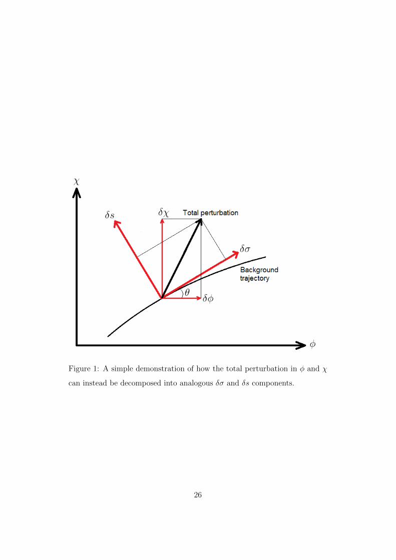
Figure 1: A simple demonstration of how the total perturbation in φ and χ

can instead be decomposed into analogous δσ and δs components.

26

minimum inflation can be driven by different fields through different direc-

tions in field space. It is, therefore, helpful to define the inflaton as being

the effective field which acts in the direction in field space of the background

trajectory — by performing an instantaneous rotation [67, 68, 69]. It is

important to note that this does not correspond to a real field, however, al-

though the final results are accurate regardless. To demonstrate this most

effectively, a two field case will be used here using φ and χ, but this can easily

be generalised to n scalar fields, as above. Figure 1 shows how a background

trajectory is no longer trapped in a one dimensional field space and can now

involve both fields acting at the same time — through simple trigonometry

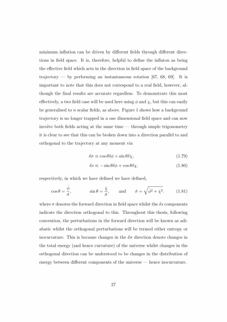
it is clear to see that this can be broken down into a direction parallel to and

orthogonal to the trajectory at any moment via

δσ ≡ cos θδφ+ sin θδχ, (1.79)

δs ≡ − sin θδφ+ cos θδχ, (1.80)

respectively, in which we have defined we have defined,

cos θ =φ

σ, sin θ =

χ

σ, and σ =

√φ2 + χ2. (1.81)

where σ denotes the forward direction in field space whilst the δs components

indicate the direction orthogonal to this. Throughout this thesis, following

convention, the perturbations in the forward direction will be known as adi-

abatic whilst the orthogonal perturbations will be termed either entropy or

isocurvature. This is because changes in the δσ direction denote changes in

the total energy (and hence curvature) of the universe whilst changes in the

orthogonal direction can be understood to be changes in the distribution of

energy between different components of the universe — hence isocurvature.

27

1.7.2 The Curvaton Scenario

Building on the use of multiple fields to both drive inflation and seed the

density perturbations — another option is to allow two fields to do each of

these respectively, rather than both together. This can be achieved through a

usual inflationary regime driven by the inflaton, φ, followed by the subsequent

decay of an otherwise inactive field — the curvaton, σ — which seeds the

perturbations [70, 71, 72, 73]. Utilising the multiple fields in this way greatly

frees up the properties of the inflaton as we no longer need to include the

observational constraints imposed upon it and can simply attach these to the

secondary field instead, although the result of this is to lessen the predictive

qualities of inflation itself. In general, the curvaton is a long lived field

which has a sub-dominant energy density throughout the inflationary epoch

and, in the standard case, is solely responsible for generating the curvature

perturbation. Some of these definitions can be relaxed, however, leading

to situations where part of the curvature perturbation still results from the

inflaton — and the precise magnitude of the curvaton’s subdominance can

easily be varied to result in a secondary period of inflation driven by the

curvaton before its decay [74, 75, 76]. We will look in more detail at the

curvaton scenario once we have studied the perturbations in section 2, in

order to understand quantitatively how the mechanism works.

1.7.3 Further Extensions?

Beyond multiple fields, two further examples of extensions to the inflation-

ary paradigm will be considered in this thesis, namely inflation with non-

canonical kinetic terms [68, 69, 77, 78, 79, 80] and inflation coupled to grav-

ity via the Ricci scalar (also known as a subset of scalar-tensor theories)

[81, 82, 83, 84, 85, 86] — both of which introduce additional room to manoeu-

28

vre in terms of building an inflationary model consistent with observations

and both of which are also natural extensions of general relativity motivated

by more fundamental theories, such as string theory [87] and supergravity

[28].

To begin with, we write down the action of a single scalar field coupled

to gravity via f(φ), as viewed in the Jordan frame,

S =1

8πG∗

∫d4x√−g(f(φ)R

2− gµν∇µφ∇νφ

2− V (φ)

)+ Sm[gµν ;matter],

(1.82)

where G∗ is known as the ‘bare’ gravitational constant and Sm is the matter

action which can be assumed to be free of additional couplings (ie. coupled

only to the metric and not additionally coupled to the scalar fields). We also

neglect an additional potential coupling in the kinetic term which is related

to the Brans-Dicke parameterisation [82]. In this frame all measurements

and observations take their usual form and interpretation because the matter

fields couple to the metric in the usual way, without an additional dependence

on the scalar field, whilst the effective gravitational constant can vary —

hence the usage of G∗ rather than G in the action. Just as in the standard

case, the action can be varied with respect to the metric and scalar field

to produce modified Einstein and Klein-Gordon equations respectively —

although we will come to look at these in more detail later on. As already

hinted at, the conservation equations of the matter fields take their usual

form due to the lack of explicit additional coupling to the fields.

It is now interesting to move from one conformal frame to another, from

the Jordan frame to the Einstein frame, to see that these two extensions —

the non-canonical kinetic terms and non-minimal coupling — are inextricably

29

linked. By performing a conformal transformation on the metric, given by

g∗µν = f(φ)gµν , (1.83)

we find that the action becomes [88],

S =1

8πG∗

∫d4x√−g∗

(R∗2− 3

4

gµν∗ ∇∗µf(φ)∇∗νf(φ)

f 2(φ)−gµν∗ ∇∗µφ∇∗νφ

2f(φ)− V (φ)

f 2(φ)

)+Sm[f(φ)g∗µν ;matter],

(1.84)

where all starred quantities are calculated in the Einstein frame and we can

immediately see that the gravitational terms have taken their usual form

whilst the scalar field and its potential now have non-canonical forms, de-

pendent on f(φ). In cases such as this, it is also possible to redefine the scalar

field in order to create a canonical kinetic term and a rescaled potential, but

when generalising to multi-field cases — such as those studied later — this

no longer holds unless only one of the many fields is non-minimally coupled.

Whilst the link between these two regimes is clear, it should be remembered

that both of these extensions are worth looking at in their own right, with

work into both equally well motivated with or without the other. As such,

in Chapters 3− 5 we shall consider variations of these extensions both alone

and with additional couplings.

30

31

2 Perturbations

The universe we see today, whilst smooth on the largest of scales, is rich in

structure which would be impossible to account for simply by studying the

background dynamics, whether using multiple fields or not. The structure

can be explained by classical density perturbations which were seeded by

the quantum fluctuations in the early universe — stretched by inflation to

the scales we can study today. Numerically it has been shown that with an

initial scale invariant density function it is perfectly possible to recover the

statistical properties observed in large scale structures today [89] — and as

such, the idea is well founded. Cosmological perturbation theory is a method

to describe and track how these fluctuations came to be in the first place, in

terms of perturbations in the scalar fields and metric, and whilst much work

has been done on this to second order [90, 91, 92, 93, 94, 95, 96] it is only

necessary to study the linear perturbations here.

Studying the perturbations in full would require us to take into account

the curvature of space, but instead we shall just look at the flat FLRW

metric on the basis that it demonstrates all the key points and is relatively

easy to generalise to curved spaces — whilst making some of the mathematics

considerably more concise, not least in now solely being able to use partial

derivatives in place of the covariant counterparts. We begin by splitting the

metric up into its background part, gµν , and its perturbed part, δgµν , such

that

gµν(τ, xi) = gµν(τ) + δgµν(τ, x

i) (2.1)

where the most general perturbation to this metric takes the following form

(working, for now, in conformal time defined by τ =∫ t

0dt/a),

ds2 = a2(τ)[−(1 + 2A)dτ 2 + 2Bidx

idτ + (δij + hij)dxidxj

], (2.2)

32

where the evolution of A,Bi and hij can be calculated from the Einstein

equations (constraints and perturbed equations of motion — which we come

to later). It is then necessary to split the perturbations into their scalar, vec-

tor and tensor components via what is known as SVT decomposition. This

technique is well justified both mathematically and physically and makes

any calculations considerably easier. At linear order, the scalar, vector and

tensor perturbations are completely independent of one another so it is pos-

sible to study each component individually — a fact that becomes especially

useful when one considers the implications of each type of perturbation on

the physical universe. Scalar perturbations are the only ones which can

cause the gravitational collapse necessary to form structure in the universe,

via their effect on the distribution of energy, vector perturbations represent

vorticity in the fields which inevitably tends towards zero as the universe

expands (although using higher order perturbation theory, this is no longer

true on small scales [97]) — becoming cosmologically irrelevant, whilst ten-

sor perturbations become the much sought after gravitational waves. SVT

decomposition is a means of decomposing the vector, Bi as

Bi = ∂iB + Bi, (2.3)

where ∂iB is the gradient of a scalar and Bi is a divergenceless vector. Sim-

ilarly, the tensor hij can be decomposed as follows [28],

hij = 2Cδij + 2∂i∂jE + 2∂(iEj) + 2Eij. (2.4)

It is important to note the following constraints,

∂iBi = 0, (2.5)

∂iEj = ∂jEi = 0, (2.6)

∂iEij = 0 and (2.7)

Eii = 0, (2.8)

33

resulting from the fact that Bi and Ei are divergenceless vectors and Eij

is a traceless, transverse tensor. We have also made use of the indices on

the linear order perturbations being raised or lowered by the unperturbed

spatial metric, in flat space, δij. We now see that in total we have 10 degrees

of freedom:

• 4 scalars — A,B,C and E.

• 2 vectors — Bi and Ei contributing two degrees of freedom apiece.

• 1 tensor — Eij also contributing two degrees of freedom.

The number of degrees of freedom leads onto an important point which has

so far been ignored, in that it turns out that some of these degrees of freedom

are unavoidable but some are merely due to a choice of coordinate system.

It is therefore necessary to now look at gauge choice and transformations —

which describe the mapping of one coordinate system onto another.

2.1 Gauges

When defining the perturbed metric, gµν (dropping the explicit space-time

dependences noted in Eq. (2.1)), in terms of the background component, gµν ,

and perturbed component, δgµν , we have assumed that these perturbations

are small and, therefore, that the full metric is still close to the unperturbed

FLRW metric. It is therefore possible, in principle, to compare the true

(perturbed) value at any space-time point to an equivalent value on the

background — but in general relativity there is no unique translation in

terms of identifying points between these two space-times, which introduces

some somewhat arbitrary degrees of freedom. This can be demonstrated by

taking a step back and considering a change of coordinate system on the

34

background metric, with the new coordinates defined by

yi = xi − ξi(xj, τ), (2.9)

where, if ξi(xj, τ) is small, it is useful to consider the similarity between it

and the perturbations about the background metric, δgµν . This results in a

line element mapped onto the new coordinate system given by

ds2 = a2(τ)[−dτ 2 + 2ξ′idy

idτ + (δij + 2∂(iξj))dyidyj

](2.10)

where it is now obvious that we have two terms that can be identified with

two of those found in the perturbed metric as Bi = ξ′i and Ei = ξi but in fact

have nothing to do with the cosmological perturbations at all and simply arise

as a consequence of our coordinate transformation. As such, it can be seen

that not all degrees of freedom are physical, and we need to find a method of

extracting those that are — either by more carefully considering our choice

of gauge to work in, which we shall come to later, or by constructing gauge

invariant variables that correspond to the physical degrees of freedom.

Similarly to before, but in slightly more detail, we will introduce a small

change to the coordinates using the vector ξµ,

xµ → xµ − ξµ (2.11)

which can in turn be broken down into its time component, ξ0 — a scalar

we shall now label T , and spatial component, ξi. ξi can also be decomposed

into its vector and scalar parts as ξi = ∂iL + Li. Under this coordinate

transformation, the metric can be shown to transform as [45, 98, 99]

δgµν = δgµν + (∂ρgµν)ξρ + (∂µξ

ρ)gρν + (∂νξσ)gµσ (2.12)

which we can now apply to the explicitly perturbed metric defined in Equa-

tions (2.2) and (2.4). Note that for the rest of this section, we denote a

derivative with respect to conformal time, ∂0X, as X ′ and H = a′/a.

35

Looking individually at each of the perturbed components, we see that

δg00 = −2a2A (2.13)

= δg00 + ∂ρg00ξρ + ∂0ξ

ρgρ0 + ∂0ξσg0σ (2.14)

= δg00 + ∂0g00ξ0 + 2∂0ξ

0g00 + 2∂0ξigi0 (2.15)

= −2a2A+ 2a2HT + 2a2T ′ (2.16)

and it becomes obvious that the first metric perturbation variable itself trans-

forms as

A→ A+ T ′ +HT (2.17)

Following the same method for the i0 and ij components we find

Bi → Bi − ∂iT + L′i (2.18)

hij → hij + ∂iLj + ∂jLi + 2HT. (2.19)

After further decomposing these into SVT parts and dropping the tildes to

simplify notation of the vectors, we can in total write out the scalar trans-

formations

A→ A+ T ′ +HT, B → B − T + L′,

C → C +HT, E → E + L, (2.20)

the vector transformations

Bi → Bi + Li′, Ei → Ei + Li (2.21)

and, for completeness, the tensor transformation

Eij → Eij. (2.22)

36

It is possible to create combinations of these perturbation variables which do

not change under coordinate transformation and are therefore gauge invari-

ant, namely, the Bardeen potentials [100]

Φ ≡ A+H(B − E ′) + (B − E ′)′ and Ψ ≡ −C −H(B − E ′), (2.23)

along with the vector and tensor variables

Φi ≡ Ei′ − Bi and Eij, (2.24)

respectively. By reparameterising in this way, the degrees of freedom have

been reduced from 10 to 6 and now directly relate to the real perturbations in

space-time. Now we have seen that it is possible to construct such quantities

in a general sense, an alternative approach is to specify a gauge from the

outset and avoid having to reconstruct the invariant variables later on. This

is possible in a number of ways, via gauge choices such as the:

Comoving gauge where the velocity of the matter fluid is set to zero —

commonly in terms of the total matter present but occasionally, if spec-

ified, in terms of a single fluid [101, 102].

Flat gauge where the curvature perturbation (defined shortly) vanishes on

spatial hypersurfaces [67, 103].

Synchronous gauge where every point corresponds to a free falling ob-

server — which is generally used for historic purposes but has some

problems in terms of not being a truly fixed gauge and hence has some

complex interpretations for modes greater than the horizon size [98].

Longitudinal/Newtonian gauge which sets the scalar metric perturba-

tions to be diagonal. We will look at this choice of gauge in a little

37

more detail as we often come to use it in subsequent work. In diago-

nalising the perturbed metric, it is necessary to set E = B = 0 (which

can be achieved by choosing ξ = −E and ξ0 = −B + E ′), in which

case the Bardeen potentials become equivalent to the remaining metric

perturbations

Φ = A (2.25)

Ψ = −C (2.26)

and the longitudinal line element becomes

ds2 = a2(τ)[−(1 + 2Φ)dτ 2 + (1− 2Ψ)δijdx

idxj]

(2.27)

In this gauge, Ψ comes to represent the curvature perturbation on

constant time hypersurfaces and for perfect fluids, where anisotropic

stress vanishes, it is possible to show that Φ = Ψ as a result of Einstein’s

equations (Eq. (2.45)).

2.2 Other perturbed quantities

The perturbations above can then be used to calculate the Einstein tensor

via the Christoffel symbols and Ricci tensor to give, at first order in the

perturbations,

δGµν = δRµν −1

2δgµνR−

1

2gµνδR, (2.28)

38

where δgµν can be easily read off from the metric and we are now working in

the Newtonian gauge, in this case Eq. (2.27), and [45, 46],

δR00 = ∂i∂iΦ + 3Ψ′′ + 3HΨ′ − 3HΨ′,

δR0i = 2∂iΨ′ + 2H∂iΦ,

δRij =

(−HΦ′ − 5HΨ′ −

(2a′′

a+ 2H2

)(Φ + Ψ)−Ψ′′ + ∂k∂

kΨ

)δij

+ ∂i∂j(Ψ− Φ). (2.29)

We can then find that

δR =1

a2

(−2∂i∂

iΦ− 6Ψ′′ − 6HΦ′ − 18HΨ′ − 12a′′

aΦ + 4∂i∂

iΨ

). (2.30)

The components of the Einstein tensor are then given by,

δG00 = −6HΨ′ + 2∂i∂iΨ,

δG0i = 2∂iΨ′ + 2H∂iΦ,

δGij =(

2HΦ′ + 4HΨ′ + 4a′′

aΦ− 2H2Φ + 4

a′′

aΨ− 2H2Ψ

+ 2Ψ′′ − ∂k∂kΨ + ∂k∂kΦ)δij + ∂i∂j(Ψ− Φ). (2.31)

We have now come to understand how the perturbations affect the space-

time itself, so the next step is to link this to the other components of the

universe by perturbing the Einstein equations (Eq. (1.5)) and taking a look

only at, for now, the perturbed scalar components,

δGµν = 8πGδTµν (2.32)

where, as in the unperturbed case, δT 00 = −δρ, δT ij = δpδij and the momen-

tum perturbation is defined as δT 0i = δqi — which can be decomposed into

scalar and vector parts, leaving the scalar part as ∂iδq. From this point on

we will be working in terms of the Fourier modes of the perturbations, k,

39

introduced earlier but will drop the subscripts (ie. φk → φ) in order to sim-

plify the equations, the main effect of this being the ability to replace ∇2

with −k2. Anyway, the scalar fields can be similarly perturbed via

φ(x, t) = φ(t) + δφ(x, t), (2.33)

to give the stress energy tensor of the scalar field as

δTµν = 2∂(νφ∂µ)δφ−(

1

2gαβ∂αφ∂βφ+ V

)δgµν

− gµν(

1

2δgαβ∂αφ∂βφ+ gαβ∂αδφ∂βφ+ Vφδφ

), (2.34)

with the components (with an implied sum over the multi-field subscript, I)

a2δT 00 = −φ′Iδφ′I + φ′2I Φ + a2VIδφI , (2.35)

a2δT 0i = −∂i(φ′IδφI , ) (2.36)

a2δT ij = δij(φ′Iδφ

′I − φ′2I Φ− a2VIδφI

). (2.37)

The scalar field perturbation itself, it should be noted, transforms with gauge

changes in the following way. By taking an arbitrary scalar quantity, f(xµ),

introducing the small coordinate shift used before and Taylor expanding —

we get

f(xµ − ξµ) ≈ f(xµ)− ∂µf(xµ)ξµ, (2.38)

only it is clear that ˜f(xµ) = f(xµ) at background level, and therefore by

combining this with Eq. (2.38) we can see that

f(xµ)→ f(xµ) + ∂µf(xµ)ξµ, (2.39)

So for the perturbations in φ, we have

δφ→ δφ+ φ′T (2.40)

40

and similarly for δρ and δp.

Using the perturbed expressions for Gµν (Eq. (2.31)) we can now equate

the scalar field perturbations to the gravitational ones via their equivalent

components in the Einstein tensor,

∇2Ψ− 3H(Ψ′ +HΦ) = 4πG(φ′Iδφ

′I − φ′2I Φ + a2VIδφI

), (2.41)

Ψ′ +HΦ = 4πGφ′IδφI , (2.42)

Ψ′′ + 2HΨ′ +HΦ′ + Φ(2H′ +H2)

+∇2 (Φ−Ψ)

2= 4πG

(φ′Iδφ

′I − φ′2I Φ− a2VIδφI

), (2.43)

whilst the fields themselves evolve according to the perturbed Klein-Gordon

equation

δφ′′I + 2Hδφ′I −∇2δφI + a2VIJδφJ = −2a2VIΦ + φ′I(Φ′ + 3Ψ′). (2.44)

We also have the two constraint equations coming from the off-diagonal parts

of the Einstein tensor, given by

Ψ− Φ = 8πGpa2Π and ∇2Ψ = 4πGa2δρm (2.45)

where δρm is the gauge invariant comoving density perturbation (δρm =

δρ − 3Hδq) [57] and Π is the anisotropic stress that is defined by these

off-diagonal components. Finally, by considering the matter conservation,

∇µTµν = 0, we can find the conservation equation of fluids in the universe

— with the first order perturbation equation being [104]

δρ = −3H(δρ+ δp)− ∇2

a2δq + 3(ρ+ p)Ψ, (2.46)

in the longitudinal gauge.

Looking briefly at the vector modes — we can see that

Φ′i + 2HΦi = Pa2πi, (2.47)

41

where πi represents the non-isotropic stress, P is the pressure and Φ′i is defined

in Eq. (2.24). In the regime of vanishing πi, which is almost always the case,

it is clear that these modes decay as a−2 and so play no further role in any

observational constraints. Similarly, in the absence of anisotropic stress, the

tensor perturbations reduce to

E ′′ij + 2HE ′ij − (∇2 − 2κ2)Eij = 0, (2.48)

where κ denotes the spatial curvature.

2.3 Returning to the observables

With all of these perturbed quantities, it is now important to remind our-

selves of which we need to keep track of and how they relate to observations.

The most important of all is the curvature perturbation which is responsible

for seeding structure formation — but even this can have various definitions,

which shall be considered below. We can start by considering the spatial

curvature found by contracting the spatial components of the Ricci tensor

with the metric, R(3) = gijRij which results in

R(3) = −4∇2

a2C (2.49)

on a constant τ hypersurface. We have already seen that C is not a gauge

invariant quantity though, so by changing the slicing of the constant time

hypersurface by the small amount, δτ , we find via Eq. (2.11) and Eq. (2.20),

C → C +Hδτ. (2.50)

If we now move to a comoving slicing, where δφcom = δφ− φ′δτ = 0 we can

then show that [46],

δτ =δφ

φ′, (2.51)

42

since we are working on a constant time hypersurface. As such, looking back

at the curvature perturbation, C, we can now see that it transforms as

C → C +Hδφφ′. (2.52)

Finally, we can now define the comoving curvature perturbation — which is

gauge invariant by construction — as,

R = −C +Hδφφ′

(2.53)

Following the same argument, but now with a uniform energy density slicing

such that δρ = 0, we can also use

δτ =δρ

ρ′, (2.54)

to derive another important quantity — the uniform energy density curvature

perturbation,

ζ = C −Hδρρ. (2.55)

We can see that these two variants of the curvature perturbation look very

similar and, in fact, in certain conditions coincide as R = −ζ. This is the

case both in single field slow roll inflation when δρ/ρ′ ∼ δφ/φ′ and on super-

horizon scales, which shall be demonstrated below. If we relate R to ζ via

R = −ζ +Hδρmρ′

, (2.56)

where δρm is the gauge invariant comoving density perturbation (= δρ −

3Hδq) and use Eq. (2.45) to get

R = −ζ +H ∇2Ψ

4πGa2ρ′, (2.57)

where it is clear that on large scales the second term becomes negligible as

in Fourier space, ∇2Ψ → −k2Ψ and the quantity k2/a2 → 0. In general, it

43

is these two quantities which are measured in terms of their power spectra,

PR or Pζ — often interchangeably.

Thus far we have only looked at these results using the simplest of cases: a

single scalar field. In the (very natural) scenario that there are multiple scalar

fields playing a role there will not only be curvature (adiabatic) perturbations,

but also isocurvature (entropy) perturbations, as briefly mentioned in Section

1.7.1. Whilst we look more carefully at this scenario in Chapter 3, a few

important results will be listed here. The pressure perturbation can, in any

gauge, be split into two components — adiabatic and non-adiabatic,

δp = c2sδρ+ p

(δp

p− δρ

ρ

)= c2

sδρ+ δpnad, (2.58)

where c2s is the sound speed (≡ p/ρ) and δpnad is the non-adiabatic pressure

perturbation . Now, working in the longitudinal gauge and in terms of the

Bardeen potential, Eq. (2.55) becomes

ζ = −Ψ− H

ρδρ = −Ψ +

δρ

3(ρ+ p). (2.59)

By taking the derivative of this with respect to time and using Equations

(2.46) and (2.58) it is relatively simple to show that [86],

ζ = − H

ρ+ pδpnad −

1

3(ρ+ p)

∇2

a2δq, (2.60)

which demonstrates that the curvature perturbation can evolve in two dif-

ferent circumstances. Firstly, if the momentum perturbation is non-zero —

although this is no longer relevant on super-horizon scales due to the pres-

ence of the scale factor in the second term — and, secondly, if there is a

non-adiabatic pressure perturbation — which would result from isocurvature

perturbations in other fluids. The isocurvature perturbation itself can be de-

scribed by considering the relative entropy perturbation between two fluids

(where, in general, in a universe with n components there will be n−1 relative

44

entropy perturbations) such that we can describe the density perturbation

of fluid I on surfaces of constant ρJ via [105]

δρIJ ∝ δρI −ρ′Iρ′JδρJ , (2.61)

which leads us to define the gauge invariant relative entropy perturbation, in

conformal time so as to match up to the adiabatic equivalent (Eq. (2.57)),

as

SIJ = 3H(δρJρ′J− δρI

ρ′I

). (2.62)

2.4 The Curvaton

We now come to take another look at the curvaton scenario, but in a little

more detail using some of the preceding ideas looked at regarding pertur-

bations. To recap, the curvaton, σ, begins life as an an almost stationary

(σ = 0) field that is subdominant to the inflaton, φ, which drives inflation.

During this time, however, it picks up isocurvature perturbations which are

converted to adiabatic curvature perturbations once inflation ends and the

inflaton has decayed — when the curvaton comes to dominate the universe.

Whilst it was previously mentioned that the curvaton comes in many forms

and can include mixed cases where it doesn’t necessarily dominate the post-

inflationary universe, we will initially look solely at the simplest case — in

which we use a quadratic curvaton (V (σ) = 12m2σσ

2), a well justified assump-

tion as most of the interesting dynamics occur in a reheating stage when the

field is oscillating close to the bottom of its potential, which would be almost

quadratic here in any case.

In order for the curvaton to be roughly constant and subdominant during

inflation, we can see that we must set mσ H2 along with V (σ) V (φ),

45

where, in this example, V (φ) = 12m2φφ

2. Since the value of the curvaton is

now frozen in during the inflationary epoch, we can set σ → σ∗ which denotes

the value throughout this period. Just as for the inflaton field, the field gains

perturbations as

σ(x, t) = σ(t) + δσ(x, t), (2.63)

where, from now on, we denote the background value, σ as σ alone for sim-

plicity and it evolves following the usual background equation,

σ + 3Hσ + Vσ = 0. (2.64)

The perturbations, assuming a negligible coupling to the inflaton, follow a

modified version of the full perturbed equation, Eq. (2.44), given by [70, 106],

δσ + 3H ˙δσ +

(k2

a2+ Vσσ

)δσ = 0, (2.65)

in which the Fourier subscript of the perturbations has once again been

dropped. After horizon exit, when k2 a2H2, the vacuum fluctuation

becomes a classical perturbation and the perturbed Klein-Gordon equation

becomes identical to the background version with a Gaussian spectrum given

by

Pδσ =H2∗

4π2. (2.66)

Once inflation ends, we assume that the inflaton decays into radiation

in the usual way whose density then decreases as a−4 and eventually, when

H ≈ mσ, the curvaton rolls down to the bottom of its potential and begins

oscillating about the minimum itself — where the quadratic oscillations allow

the field to behave as pressureless matter whose energy density scales as

a−3. At this point, there are two regimes available to us depending on the

46

magnitude of the curvaton decay parameter, Γσ (= Γγσ + Γmσ , if decays occur

both to radiation and matter): the case where Hosc ∼ Γσ soon enough such

that ρσ never comes to dominate the universe over the radiation and the

case where Hosc > Γσ (where Hosc denotes H at the start of this phase) in

which ρσ loses energy much more slowly than ργ and ends up dominating

the universe before decay. The ratio of the curvaton energy density to total

energy density at the time of curvaton decay will be denoted by

rdec =ρσ

ργ + ρσ, (2.67)

and plays a key role in measuring how much of the final observables are

sourced either by the inflaton or curvaton. There are a number of other

definitions of rdec in the literature which often coincide with the version given

above, but are worth being aware of in any case. Two common alternatives

are the following,

rdec =ρσργ

and rdec =3ρσ

4ργ + 3ρσ, (2.68)

which correspond to the curvaton-radiation energy density ratio and the to-

tals including pressure of both fluids respectively. Looking more carefully at

oscillatory curvaton’s energy density, which averages out as

ρσ =1

2m2σσ

2, (2.69)

and breaking it down into its background and perturbed parts too,

ρσ → ρσ + δρσ, (2.70)

we can show that the density contrast, δ = δρ/ρ can be expanded to

δ(σ) = 2δσ

σ+δσ2

σ2. (2.71)

47

We have already seen (Equation (2.66)) that the perturbation is proportional

to H∗ so from this we can find a further constraint on the curvaton field. By

considering the case of H∗ σ∗, such that the perturbation is greater than

the background, the second term in the density contrast dominates and we are

left with a gaussian-squared quantity — which is forbidden by observation.

If, on the other hand, we take H∗ σ∗ then the first term dominates and

leaves

δ = 2δσ

σ, (2.72)

which has a flat power spectrum given by [106]

Pδ = 4Pδσσ2

=H2∗

π2σ2 1. (2.73)

Of course, there is still room to have certain intermediate cases, where

H∗ ≤ σ∗ which give small non-gaussianities in the power spectrum, but

for the time being we will continue to focus on the simplest case. Looking

towards the final curvature perturbation we now come to consider the mix

of fluids present at this time and how they each contribute to ζ. Initially, we

assume that the curvaton is sub-dominant and as such acts as an isocurvature

perturbation to the radiation fluid’s curvature perturbation. We know from

Eq. (2.60) that even on super-horizon scales this can source/enhance the

curvature perturbation via δpnad, but the precise form of this final curvature

perturbation needs a closer look. Allowing each component of the universe

to have its own curvature perturbation, ζσ and ζγ and assuming that prior

to curvaton decay ζ = ζγ ∼ 0 — working on uniform density hypersurfaces

and using Eq. (1.12) we have

ζ = −Hδρ

ρ= ζγ + ζσ =

4ργζγ + 3ρσζσ4ργ + 3ρσ

=ρσ

4ργ + 3ρσδ. (2.74)

48

In terms of rdec this can be quickly expanded to

ζ =rdec

4− rdecδ (2.75)

and we see that if the curvaton dominates (rdec = 1) then

ζ =δ

3, (2.76)

whilst if the curvaton is sub-dominant and decay (rdec 1), we have

ζ =rdecδ

4. (2.77)

Although not relevant to subsequent work here, it is also worth mention-

ing the production of isocurvature perturbations in the curvaton scenario. In

terms of the two components under consideration here, the entropy pertur-

bation prior to curvaton decay, given by Eq. (2.62), becomes

Sσγ = 3(ζσ − ζγ), (2.78)

and with the assumption used earlier, that ζγ = 0 we are left with Sσγ = 3ζσ.

For one thing, we can therefore see that the isocurvature perturbations are

correlated to the curvature ones — and also that, due to the late decaying

nature of the curvaton (after inflation) there is a mechanism for producing

primordial isocurvature perturbations even on super-horizon scales. For more

on this, see [106].

In terms of other observational quantities, just as in the usual inflationary

cases, it is relatively easy to find expressions for the spectral index and tensor-

scalar ratio. A convenient new parameterisation for this, related to the ratios

at decay (rdec) found before, is via R, defined by [107]

Pζ = P(φ)ζ + P(σ)

ζ = (1 +R)P(φ)ζ where R =

P(σ)ζ

P(φ)ζ

, (2.79)

49

where it can be shown that

R =8

9εr2dec

σ2∗, (2.80)

since [73, 108]

P(φ)ζ =

1

2ε

(H∗2π

)2

and P(σ)ζ =

r2dec

9π2

H2∗

σ2∗. (2.81)

Using this the spectral index can be written

ns − 1 = −2ε+ 2ησσ −4ε− 2ηφφ

1 +R, (2.82)

in agreement with the standard two field derivation found in [109] and where

ηAB = VAB/3H2. Quantitatively this leads to a range of spectral indices

that fit well with current data — with values of ns ∼ 0.96 for the inflaton

dominated case ranging up to ns ∼ 0.98 in the curvaton dominated case. The

tensor perturbations in these scenarios remain unaffected by the curvaton and

depend solely on the energy scale of inflation (assuming the curvaton is truly

sub-dominant). As such, the tensor power spectrum takes its usual value

(Eq. (1.71)) and the tensor-scalar ratio is modified to

r =16ε

1 +R, (2.83)

from which we can see that when the curvaton dominates and R is large the

ratio is suppressed, whilst in the event that R→ 0, when the curvaton contri-

bution to the curvature perturbation is insignificant, we retain the standard

result. Observationally, the simplest curvaton model — in which the cur-

vaton dominates the universal energy density before decay — is verging on

being ruled out due to its rather large spectral index, although many variants

remain in contention as viable alternatives and, in fact, offer an attractive

mechanism by which to minimise the ever elusive scalar-tensor ratio.

50

In addition to the summary above, there remain a couple of important

potential corrections to this scenario which have been thus far neglected —

but shall be mentioned for completeness. Firstly, the above treatment only

accounts for the perturbative decay of the curvaton and neglects the possi-

bility of preheating which would proceed similarly to the usual parametric

reheating considered for the inflaton [110]. There is a small but significant

difference though, as in the curvaton case the backreaction from the particles

produced is always important whereas in the inflaton case certain parame-

ter choices can avoid this — the result of this will then affect the initial

conditions of the subsequent usual reheating phase. Secondly, leading on

from the first point, the backreaction from the decay of the curvaton (even

perturbatively) causes correction terms in the effective potential which have

been shown to have significant consequences for the observables [72, 111].

Using the interaction term written down in the case of the inflaton earlier,

Eq. (1.38), results in two correction terms in the potential — one a quan-

tum correction (the details of which can be found in [72, 112]), ∆V (σ), and

the other a correction related to the temperature of the induced background

radiation, VT . So that the quadratic potential used here is changed to

Veff(σ) =1

2m2σσ

2 + VT (σ) + ∆V (σ), (2.84)

and the coherent oscillations of the field about the minimum are altered to

the extent that it no longer behaves as pressureless matter and the resultant

dilution due to the expansion of space is altered. The result of all this is

primarily to alter the initial parameter space that is viable in curvaton models

and hence the naturalness of any such mechanism, but can also produce

non-gaussianities from the initially gaussian perturbations, which has the

potential to help distinguish between competing models.

Ending this section, we see from Figure 2 that the standard (double

51

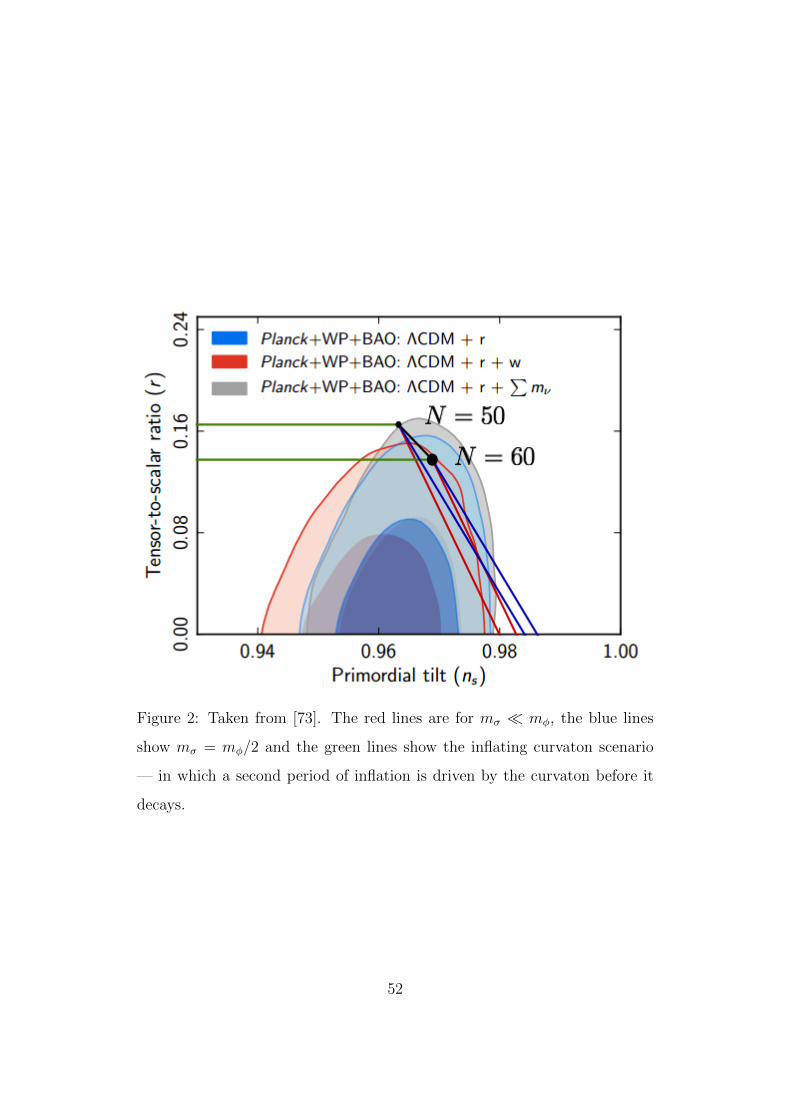
Figure 2: Taken from [73]. The red lines are for mσ mφ, the blue lines

show mσ = mφ/2 and the green lines show the inflating curvaton scenario

— in which a second period of inflation is driven by the curvaton before it

decays.

52

quadratic) curvaton is close to being ruled out by Planck — especially at

the curvaton domination end of the spectrum where ns ∼ 0.98. However,

the methodology laid out above is still perfectly valid for variations on the

simplest case — including changing either, or both, of the potentials, chang-

ing the decay parameters or even by including additional couplings between

either the fields themselves or to gravity, which we come to later.

53

54

3 Second order slow-roll with

non-canonical kinetic terms

In this Chapter we shall consider the effects on the power spectrum of multi-

field inflation with non-canonical kinetic terms using first order cosmological

perturbation theory in the slow roll regime. Previously this has been approx-

imated to leading order in the slow roll parameters [68, 69, 78] but we show

it necessary to go beyond this — to second order in the slow roll parameters

— in order to gain a useful insight into the dynamics.

With single field models, studying the evolution of the perturbations and

resultant power spectra is a relatively simple task as the perturbations be-

come frozen in as the mode of interest exits the horizon, but in multi-field

models this is no longer the case. This is because the additional degree(s)

of freedom afforded by extra dimensionality of the field space allows pertur-

bations in more than one direction — both along the background trajectory

(curvature perturbations) and orthogonal to it (isocurvature perturbations)

— which, it turns out, are not independent of one another. Isocurvature per-

turbations themselves describe the relative perturbations between the fields

present and it is already well known that they can source curvature pertur-

bations long after horizon exit (see e.g. [117, 118, 119]) — thereby adding

an additional layer of complexity when it comes to finding the final values

of the power spectra which we wish to observe today. The sourcing of the

curvature perturbation is largest when sharp turns in field space are present

and we expect this to be the case in numerous non-canonical cases.

A significant amount of work has already been done on this [120, 121, 122,

123, 124, 125, 126] making use of both the δN formalism [127, 128, 129, ?]

and the transfer matrix method [66, 69]. We use the transfer matrix method

55

and attempt to generalise the work from [68, 69, 78] which is focused solely

on the first order slow roll expansion applied to both canonical and non-

canonical cases, along with [66] in which the method is completed to second

order but only in the canonical case — to include terms second order in

slow-roll parameters in both canonical and non-canonical cases. Bringing

this expanded method to the non-canonical cases therefore seems a logical

next step. Upon calculating the relative sizes of some newly defined non-

canonical slow roll parameters from the background trajectories, we find

that this step is well motivated as such terms can easily dominate over their

standard counterparts.

The next section covers the analytics and some important derivations re-

garding commonly used quantities to second order in the slow roll parameters,

which are themselves soon defined. The bulk of the calculations must then

be split into two distinct regimes — the early time/horizon crossing regime

in which the perturbations begin well inside the horizon right through to

their exit, followed by the super-Hubble regime in which the behaviour is

significantly different. The early evolution is dominated by an explicit time

dependence in the equations of motion whilst the slow roll parameters re-

main (generally) very small, but the latter evolution is eventually dominated

purely by the growing slow roll terms. We begin with the early times regime,

in which the resultant power spectra are calculated before continuing on to

the super-Hubble regime using some of these results. The calculation itself

follows closely that of [69] but goes beyond this with the inclusion of the

second order terms. After this, the numerical procedure is introduced along

with the inflationary potentials under consideration. Finally, we come to

compare the full numerical results with those of the various approximations

— both first and second order — with a series of graphs to demonstrate

56

the success and necessity of including the additional terms, all normalised to

single field results for ease of comparison.

3.1 Non-canonical kinetic terms

The motivation for including non-standard models of inflation has already

been touched upon in the introduction to this thesis, but before proceed-

ing we will briefly recap and expand upon this. The number of light scalar

fields available in string theory is large and their dynamics often governed

by a non-trivial metric [116] — which in general leads to models of infla-

tion with non-canonical kinetic terms when transformed into the relevant

reference frame [78, 131, 132, 133, 134]. It is also possible to open up new

potentials that would otherwise be too steep to be viable by the additional

friction terms introduced by non-canonical terms in the equations of motion

[135, 136], allowing greater freedom in potential model building. There was

also previous interest in these models due to the possibility of inducing large

non-Gaussianities [137] in the inflationary spectrum, but with this now in-

creasingly constrained by Planck [48] this motivation at least is now waning.

A review and more general information can be found in [138] and [139].

It has previously been shown in [69] that it is possible to study non-

canonical inflation by approximating it in the slow roll regime and, at first

order, the qualitative dynamics of the power spectra resulting from a number

of inflationary trajectories are well captured. It was mentioned earlier how in

multifield inflation the isocurvature perturbations can source curvature per-

turbations on scales larger than the horizon, and the paper goes on to measure

this sourcing via the cross correlation coefficient, Cσs — which is then bro-

ken down into two components, the canonical (Ccσs) and non-canonical (Cncσs)

contributions. It is then clearly shown that for certain models (for example,

57

double quadratic inflation) the non-canonical contribution can be up to 3 or-

ders of magnitude greater than the canonical one. This is, however, where it

becomes clear that further work is needed — as whilst the qualitative features

of the evolution of the power spectrum are well captured, the quantitative

aspects are often underestimated at first order in slow roll, which is perfectly

understandable when the non-canonical terms can be so much larger than

their standard slow roll counterparts.

In [66] a number of canonical models have been considered to not only

next to leading order, but also briefly to next-next-order in order to give an

estimate of the accuracy of the second order approximation — and in compar-

ison to the leading order work of the previous paragraph the power spectrum

approximations have vastly improved and are now often indistinguishable

from the exact numerical comparisons. There are a couple of discrepancies,

however, such as in the case of the quartic potential which we too shall in-

vestigate later. It is expected from these results that continuing in a similar

way but with the introduction of second order non-canonical terms we can

gain a similar level of accuracy in non-standard cases and, furthermore, a

greater understanding of what dominates the contribution to the final power

spectrum and when.

3.2 Extending the analytics

The model considered here is given by the following action, in which we

introduce the specific form of the non-canonical kinetic term which couples

χ to φ:

S =

∫d4x√−g[M2

P

2R− 1

2(∂µφ)(∂µφ)− e2b(φ)

2(∂µχ)(∂µχ)− V (φ, χ)

].

(3.1)

58

We have chosen this coupling as it is commonly found after performing con-

formal transformations on cosmologies with non-standard gravitational cou-

plings [140] whilst also remaining quite general. Working in Planck units,

i.e. with MP = 1, the background motion of the fields follows the equations

φ+ 3Hφ+ Vφ = bφe2bχ2, (3.2)

χ+ (3H + 2bφφ)χ+ e−2bVχ = 0, (3.3)

which remain valid for any general function, b(φ). The Friedmann equations

then take the form

H = −1

2

[φ2 + e2bχ2

]and (3.4)

H2 =1

3

[φ2

2+e2b

2χ2 + V (φ, χ)

], (3.5)

and it should be noted that we will continue to work in the longitudinal

gauge in order to study the perturbations at linear order, defined by

ds2 = −(1 + 2Φ)dt2 + a2(1− 2Φ)dx2, (3.6)

and we break the fields down in the usual way, into their background and

perturbed components

φ(t, x) = φ(t) + δφ(t, x) and

χ(t, x) = χ(t) + δχ(t, x), (3.7)

from which we can find the perturbed Klein-Gordon equations,

δφ+ 3H ˙δφ+

(k2

a2+ Vφφ − bφφχ2e2b − 2b2

φχ2e2b

)δφ+Vφχδχ− 2bφe

2bχ ˙δχ

= 4φΦ− 2VφΦ,

δχ+ (3H + 2bφφ) ˙δχ+

(k2

a2+ e−2bVχχ

)δχ

+e−2b(Vφχ2bφVχ + 2bφφφχ

)δφ+ 2bφχ ˙δφ = 4χΦ− 2e−2bVχΦ,

(3.8)

59

and associated energy and momentum constraints,

3H(Φ +HΦ) + HΦ +k2

a2Φ = −1

2

(φ ˙δφ+ e2bχ ˙δχ+ bφe

2bχ2δφ+ Vφδφ+ Vχδχ),

Φ +HΦ =1

2

(φδφ+ e2bχδχ

), (3.9)

in which we have now begun using the Fourier components of the field per-

turbations, δφk, but drop the subscripts for clarity. Next we perform the

instantaneous rotation in the field space of φ and χ, to give

δσ ≡ cos θδφ+ sin θebδχ,

δs ≡ − sin θδφ+ cos θebδχ, (3.10)

where we have defined,

cos θ =φ

σ, sin θ =

χeb

σ, and σ =

√φ2 + e2bχ2. (3.11)

It is clear now that, as in Section 1.7.1, the δσ and δs components describe

the adiabatic and entropy perturbations respectively, whilst θ describes the

amount of curvature in the trajectory. At this point a further change of vari-

ables is necessary, and it is useful to work with the gauge invariant Mukhanov-

Sasaki variables [141, 142], defined by

Qσ ≡ δσ − σ

HΦ, (3.12)

whilst δs, is automatically gauge invariant by the Stewart–Walker lemma

[28]. Finally, the background equations can be rewritten in this new basis as

σ + 3Hσ + Vσ = 0 and

θ +Vsσ

+ bφσ sin(θ) = 0, (3.13)

and the form of the perturbation equations is now given by(Qσ

δs

)+

3H 2V,sσ

−2V,sσ

3H

(Qσ

δs

)+

k2

a21 +

Cσσ Cσs

Csσ Css

(Qσ

δs

)= 0.

(3.14)

60

The coefficients, CAB can be shown to be:

Cσσ = Vσσ −(Vsσ

)2

+ 2σVσH

+ 3σ2 − σ4

2H2− bφ

(s2θcθVσ +

(c2θ + 1

)sθVs

),

Cσs = 6HVsσ

+ 2VσVsσ2

+ 2Vσs +σVsH

+ 2bφ(s3θVσ − c3

θVs),

Csσ = −6HVsσ− 2

VσVsσ2

+σVsH

,

Css = Vss −(Vsσ

)2

+ bφ(1 + s2

θ

)cθVσ + bφc

2θsθVs − σ2

(bφφ + b2

φ

), (3.15)

where, for brevity, we denote sθ = sin(θ) and cθ = cos(θ). In deriving

this, it may be important to note the relationship between the derivatives of

the potential with respect to the fields in both frames – where it should be

pointed out that in terms of σ and δs these are no longer true derivatives,

but conveniently labeled parameters with similar properties. It is trivial to

show why this should be the case as demonstrated in [143], where ∂2σ∂χ∂φ

6=∂2σ∂φ∂χ

and ∂2s∂χ∂φ

6= ∂2s∂φ∂χ

. This is a result of these transformations merely

remaining projections of the fields rather than redefined fields themselves.

The parameters used here, are defined by,

Vσ = cθVφ + e−bsθVχ and Vs = −sθVφ + e−bcθVχ, (3.16)

along with the second derivative equivalents,

Vσσ = c2θVφφ + 2e−bsθcθVφχ + e−2bs2

θVχχ,

Vσs = sθcθVφφ + e−b(c2θ − s2

θ)Vφχe−2bsθcθVχχ and

Vss = s2θ − e−bsθcθVφφ + e−2bc2

θVφχVχχ. (3.17)

3.2.1 Slow-Roll

We define the slow roll parameters in the usual way,

ε = − H

H2and (3.18)

ηAB =VAB3H2

. (3.19)

61

However, we can no longer assume that the slow roll parameters remain

roughly constant throughout and evaluate them solely at horizon exit, instead

we must find out how they vary in time and compute their time derivatives to

second order. The expressions found are directly comparable to those derived

in [66], but with a number of additional terms describing the non-canonical

deviations from usual slow-roll. Following the definition of ξ used in [69], we

write

ξ1 =√

2εbφ and introduce (3.20)

ξ2 = 2εbφφ, (3.21)

which shall be regarded as first and second order slow roll parameters respec-

tively. The time derivatives of the slow roll parameters then become

ε = 2Hε(2ε− ησσ − ξ1s2θcθ),

˙ησσ = 2Hεησσ − 2Hη2σs − 2Hησσξ1s

2θcθ − 4Hησsξ1sθc

2θ −Hασσσ,

˙ησs = 2Hεησs +Hησsησσ −Hησsηss − 2Hηssξ1sθc2θ −Hησsξ1cθ −Hασσs,

˙ηss = 2Hεηss + 2Hη2σs − 2Hc3

θξ1ηss −Hασss and

ξ1 = 2Hεξ1 −Hξ1ησσ −Hξ21s

2θcθ +Hξ2cθ, (3.22)

where

αIJK ≡VσVIJKV 2

, (3.23)

and the full derivation can be found in the appendix, A.1. The exact pertur-

bation equations (3.15) may now themselves be expanded to second order in

the slow-roll parameters (ε, ηAB and ξ1), and the CAB coefficients become,

Cσσ = 3H2

[ησσ − 2ε+ ξ1s

2θcθ −

η2σs

3− 2ε2 +

4εησσ3

+ξ1ησs

3(sθ − 3sθc

2θ)

+5εξ1s

2θcθ

3− ξ1ησσs

2θcθ

3+ξ2

1s4θc

2θ

3

],

(3.24)

62

Cσs = 3H2

[2ησs − 2ξ1s

3θ +

2ησσησs3

− 2εξ1s3θ

3+

2ξ21c

3θs

3θ

3+

2ησsξ1cθ(s2θ − c2

θ)

3

],

(3.25)

Csσ = 3H2

[4εησs

3− 2ησσgσs

3+

2ησσξ1s3θ

3− 4εξ1s

3θ

3− 2ησsξ1s

2θcθ

3+

2ξ21s

5θcθ

3

],

(3.26)

Css = 3H2

[ηss − ξ1(1 + s2

θ)cθ −η2σs

3+ξ2

1c2θ(s

4θ − 1)

3+ησsξ1sθ(1 + s2

θ)

3

+ησσξ1cθ(1 + s2

θ)

3− εξ1cθ(1 + s2

θ)

3− ξ2

3

],

(3.27)

and it is in this form that we shall now use them. From this point the

approximation requires splitting into two distinct regimes — that of horizon

crossing followed by that of the subsequent evolution, which begins a few

efolds after horizon crossing — due to the significantly different dominant

factors in the evolution during the two time periods. Before moving onto

this, however, it is necessary to take a look at how the scale factor behaves

in terms of the slow-roll parameters.

3.2.2 The evolution of the scale factor

In many of the evolution equations describing the perturbations and, eventu-

ally, power spectra we will require an expression for various forms of a, a′ and

a′′ that has been expanded to an equivalent degree in the slow-roll parame-

ters to the rest of the equations. As such we need to calculate expressions

up to second order to be used later, we can can do this beginning from the

standard expression, working in conformal time,

a(τ) = − 1

Hτ

1

(1− ε−O2)≈ − 1

Hτ(1 + ε+O2), (3.28)

where O2 is used to denote the as yet unknown second order terms and take

various values as we proceed. Taking the derivative of this with respect to

63

cosmic time and dropping higher order terms as we proceed, we get

a(τ) =H

H2τ(1 + ε+O2) +

τ

Hτ 2(1 + ε+O2)− ε

Hτ

=−ετ

(1 + ε+O2) +1

a(τ)Hτ 2(1 + ε+O2)− ε

Hτ

=−ετ

(1 + ε+O2)− 1

τ− ε

Hτ(3.29)

where in order to get the last line we have made use of Eq. (3.28). Due to

the multiplication by ε in the first term and the cancellation in the middle

term, all dependence on the unknown O2 has dropped out, so we now have

a(τ) = −1

τ

(1 + ε+ ε2 +

ε

H

). (3.30)

Returning to Eq. (3.28), we can simply multiply through by H to leave an

alternate expression for a as

a(τ) ≈ −1

τ(1 + ε+O2), (3.31)

which can now be compared to that found with Eq. (3.30). It is immediately

obvious that the higher order terms must be given by

O2 ≡ ε2 +ε

H. (3.32)

The expansion of a is therefore

a(τ) = − 1

Hτ

(1 + ε+ ε2 +

ε

H

). (3.33)

Going further, the Hubble parameter itself can be expanded about its

value at horizon crossing — we can start by writing H = H∗+Hδt and using

the dt = da/Ha. Integrating this gives

t− t∗ =1

H∗(ln(a)− ln(a∗)) , (3.34)

64

such that

H = H∗ +H∗H∗

(ln(a)− ln(a∗)) = H∗

(1− ε ln

(a

a∗

)). (3.35)

At horizon crossing, k = a∗H∗ and using the zeroth order (treating the

logarithm term as ∼ O(1)) expansion of a, a = (H∗τ)−1, this can be rewritten

H = H∗(1 + ε ln(−kτ)), (3.36)

which can now be inserted back into Eq. (3.33) to give the full second order

expansion around horizon crossing,

a(τ) = − 1

H∗τ

(1 + ε+ ε2 +

ε

H

)(1− ε ln(−kτ))

= − 1

H∗τ

(1 + ε+ ε2 +

ε

H− ε ln(−kτ)

). (3.37)

Finally, the expansion of ε can be inserted from Eq. (3.22) in order to find

the full expression,

a(τ) = − 1

H∗τ

(1 + ε+ 5ε2 − 2εησσ − 2εξ1s

2θcθ − ε ln(−kτ)

). (3.38)

As well as requiring the expansion of a(τ) itself, we often find a′′/a when

working on the perturbation equations in conformal time. Proceeding using

an overdot and a dash to denote derivatives with respect to cosmic and confor-

mal time respectively, this calculation will now be summarised. Throughout,

higher order terms are dropped when necessary but the value of O2 found in

Eq. (3.32) shall continue to be used to shorten the working — so we begin

with the relation

a′ = aa =1

τ(1 + ε+O2)

1

Hτ(1 + ε+O2)

=1

Hτ 2(1 + 2ε+ ε2 + 2O2). (3.39)

65

We also know that

∂

∂τ≡ a

∂

∂t→ a′′ = aa′ (3.40)

so

a′′

a= a′ =

∂

∂t

(1

Hτ 2(1 + 2ε+ ε2 + 2O2)

)= − H

H2τ 2(1 + 2ε+ ε2 + 2O2)− 2τ

Hτ 3(1 + 2ε+ ε2 + 2O2) +

1

Hτ 2(2ε)

=ε

τ 2(1 + 2ε)− 2

aHτ 3(1 + 2ε+ ε2 + 2O2) +

2ε

Hτ 2

=1

τ 2

(ε+ 2ε2 + 2

1 + 2ε+ ε2 + 2O2

1 + ε+O2

+ 2ε

H

)=

1

τ 2

(2 + 3ε+ 2ε2 + 2ε/H + 2O2

), (3.41)

into which we can then resubstitute the expressions for O2 (Eq. (3.32)) and

ε (Eq. (3.22)) to give

a′′

a=

1

τ 2(2 + 3ε+ 20ε2 − 8εησσ − 8εξ1s

2θcθ). (3.42)

3.2.3 Horizon Crossing

Returning to the perturbation equations themselves and rescaling the fields

as uσ = aQσ and us = aδs we can rewrite Eq’s. (3.14) in conformal time to

find [(d2

dτ 2+ k2 − a′′

a

)1 + 2E

1

τ

d

dτ+ M

1

τ 2

](uσus

)= 0, (3.43)

where

E =

0 aVsσ

−aVsσ

0

and (3.44)

M =

a2Cσσ a2Cσs − 2a′Vsσ

a2Csσ + 2a′Vsσ

a2Css

. (3.45)

66

Then, we can proceed with the help of the rotation given by

R =

cos Θ − sin Θ

sin Θ cos Θ

, (3.46)

in which the angle, Θ, is chosen to allow the perturbation equations to be

independent for a given mode at Hubble radius crossing. For completeness,

the explicit value of Θ can be calculated from [124] and if, for the moment,

we neglect the a′′

a-term — it is possible to once more rewrite Eq. (3.43),

which is of the form u′′ + 2Lu′ + Mu = 0, using u = Rv as

v′′ + R−1(−L2 − L′ + M)Rv = v′′ + R−1QRv

= 0,(3.47)

where the matrix, Q is labeled

Q =

AQ BQ

CQ DQ

, (3.48)

and the coefficients are given by summing the equivalent matrix coefficients

in the following way,

AQ = M(1,1) − E2(1,1), BQ = M(1,2) + E(1,2) + E(1,2),

CQ = M(2,1) + E(2,1) + E(2,1), DQ = M(2,2) − E2(2,2), (3.49)

in which null valued coefficients have meant certain contributions to Q have

been left out above. The fully expanded version of the coefficients is found

to be

AQ = 3ησσ − 6ε+ 3ξ1s2θcθ + 10εησσ − 18ε2 + 11εξ1s

2θcθ

− ησσξ1s2θcθ + ξ2

1s4θ − ησsξ1sθ(1 + c2

θ),

BQ = 3ησs − 3ξ1s3θ + 8εησs − 9εξ1s

3θ + ησσξ1s

3θ − ησsξ1c

3θ + ξ2

1s3θcθ,

CQ = 3ησs − 3ξ1s3θ + 8εησs − 9εξ1s

3θ + ησσξ1s

3θ − ησsξ1c

3θ + ξ2

1s3θcθ,

DQ = 3ηss − 3ξ1cθ(1 + s2θ) + 6εηss − 7εξ1cθ(1 + s2

θ) + ησσξ1cθ(1 + s2θ)

+ ησsξ1sθc2θ + ξ2

1(s4θ − c2

θ)− ξ2.

(3.50)

67

Next we must diagonalise Q using the value of the rotation matrix, R, eval-

uated at Hubble radius crossing (denoted by the subscript ∗) to give R∗ and

the associated angle, Θ∗,

R−1∗ QR∗ =

λ1∗ X

Y λ2∗

, (3.51)

in which we can set X = Y = 0 in order to find the expression for λ∗:

λ1,2∗ =AQ∗ +DQ∗

2± AQ∗ −DQ∗

2

√1 +

4B2Q∗

(AQ∗ −DQ∗)2. (3.52)

A more convenient representation of the λ∗’s can be found by explicitly using

the rotation matrix, however. After a bit of algebra we can arrive at the

following expressions which will come in handy later,

λ1∗ + λ2∗ = AQ∗ +DQ∗,

(λ1∗ − λ2∗) sin 2Θ∗ = 2BQ∗,

(λ1∗ − λ2∗) cos 2Θ∗ = AQ∗ −DQ∗,

λ21∗ + λ2

2∗ = A2Q∗ +D2

Q∗ + 2B2Q∗. (3.53)

In doing this we have assumed that the slow roll parameters here are small

enough to allow us to compute this rotation using purely horizon-crossing

values. This assumption will be demonstrated and justified a little later on

when we come to the numerics. Following the equivalent calculation in [69],

by performing another change of variable, w = R−1∗ vR∗ we can rewrite the

above system of equations, Eq. (3.47), as two independent equations in w:

w′′A +

[k2 − 1

τ 2(2 + 3λA∗)

]wA = 0, (3.54)

which has two solutions given by the general form,

wA =√−τ[A(k)H(1)

µA+B(k)H(2)

µA

]. (3.55)

68

where H(1,2)µA is a Hankel function of the first or second kind respectively,

of order µA — where µ2A ≥ 0. It is then possible to define a vacuum that

corresponds to the Bunch-Davies vacuum by enforcing that as τ → −∞ only

the positive frequency modes exist. The appropriate, positive solution, is

then given by

wA ∝√π

2

√−τH(1)

µA(−kτ). (3.56)

The µA can now be expanded to second order as µA ≈ 32

+ λA∗ −λ2A∗3

. We

have also now moved from λ∗ to λ∗ using the relation,

λA∗ = ε∗ +20ε2∗

3− 8ε∗ησσ∗

3− 8ε∗ξ1∗s

2θ∗cθ∗

3− λA∗

3, (3.57)

which takes into account the a′′

aterm omitted earlier, in Eq. (3.42). Going

back to the definition of the power spectra, using

〈QA(k)QB(k′)〉 = δ(3)(k + k′)2π2

k3PAB(|k|), (3.58)

along with the relations — coming from the rotations used previously to

equate Qσ and δs to w1 and w2, respectively,

a2⟨Q†σQσ

⟩= cos2 Θ∗

⟨w†1w1

⟩+ sin2 Θ∗

⟨w†2w2

⟩, (3.59)

a2⟨δs†δs

⟩= sin2 Θ∗

⟨w†1w1

⟩+ cos2 Θ∗

⟨w†2w2

⟩, (3.60)

a2⟨δs†Qσ

⟩=

sin 2Θ∗2

(⟨w†1w1

⟩−⟨w†2w2

⟩), (3.61)

we see that we need to find the correlation functions associated with wA,

where we now relabel −kτ = x,⟨w†AwA

⟩=−τπ

4| H(1)

µA∗(x) |2 . (3.62)

We do this by applying a Taylor expansion,

f(y) ≈ f(z) + f ′(z)(y − z) +f ′′(y)

2(y − z)2 + ..., (3.63)

69

to the Hankel function, where a dash denotes the derivative with respect to

µ and we have set z = 3/2. For the time being we will drop the explicit

argument, x, along with the horizon crossing subscript and order of the

Hankel functions in order to shorten some lengthy expressions — it should

be understood, however, that the following is still strictly for use in the

horizon crossing regime only. This gives

HµA ≈ H3/2 +H ′3/2(µA − 3/2) +H ′′3/2(µA − 3/2)2

2

= H3/2 +H ′3/2(λA − λ2A/3) +H ′′3/2

(λA − λ2A/3)2

2

= H3/2 +H ′3/2(λA − λ2A/3) +H ′′3/2

λ2A

2, (3.64)

up to second order. To further clarify, it should be remembered that the

derivatives are with respect to the order of the function in the above equa-

tions, for example,

H ′3/2 =dHµ(x)

dµ

∣∣∣∣µ=3/2

. (3.65)

What is actually required here though, is | HµA |2, so we have

| HµA |2 =

(H3/2 +H ′3/2

(λA −

λ2A

3

)+H ′′3/2

λ2A

2

)2

= H23/2 + 2H3/2H

′3/2

(λA −

λ2A

3

)+ λ2

AH3/2H′′3/2 +H ′23/2

(λA −

λ2A

3

)

=| H3/2 |21 + 2

(λA −

λ2A

3

)H ′3/2H3/2

+ λ2A

H ′′3/2H3/2

+ λ2A

(H ′3/2H3/2

)2 .(3.66)

Collecting terms with respect to λA, we then find

| HµA |2 = H23/2

1 + 2λAH ′3/2H3/2

+ λ2A

H ′′3/2H3/2

+

(H ′3/2H3/2

)2

− 2

3

H ′3/2H3/2

,(3.67)

70

which we shall write, in full, as

| H(1)µA∗(x) |2=| H(1)

3/2∗(x) |2[1 + 2λA∗f(x) + λ2

A∗g(x)]

(3.68)

where

f(x) = Re

1

H(1)3/2(x)

dH(1)µ (x)

dµ

∣∣∣∣∣µ=3/2

and (3.69)

g(x) = Re

1

H(1)3/2(x)

d2H(1)µ (x)

dµ2

∣∣∣∣∣µ=3/2

+

1

H(1)3/2(x)

dH(1)µ (x)

dµ

∣∣∣∣∣µ=3/2

2

− 2

3

1

H(1)3/2(x)

dH(1)µ (x)

dµ

∣∣∣∣∣µ=3/2

. (3.70)

The functions f(x) and g(x) can be evaluated as x→ 0 as

f(x) = 2− γ − ln 2− lnx, (3.71)

6g(x) = 16 + 24 γ ln (2) + 12 (ln (2))2 − 44 ln (2) + 3 π2 − 44 γ + 12 γ2

+ 24 ln (x) γ + 24 ln (x) ln (2)− 44 ln (x) + 12 (ln (x))2 .

(3.72)

in which γ is the Euler-Mascheroni constant (' 0.5772). These evaluations

were done numerically, the details of which can be found in Appendix A.2.

Finally, the Hankel function itself needs to be evaluated at µA = 3/2. Taking

the recursion relation for generic Bessel functions, Zν(z),

zZν−1 + zZν+1 = 2νZν , (3.73)

we can find that

H(1)3/2(x) =

1

xH

(1)1/2(x)−H(1)

−1/2(x). (3.74)

The Hankel function itself, of the first kind (the only kind used here — de-

noted by H(1) but with the superscript often dropped for clarity in notation)

71

can easily be found from its definition, but it is useful to take the standard

asymptotic result (valid as x→∞),

H(1)µ (x) =

√2

πxei(x−

π2µ−π

4), (3.75)

which in this case can be used to find,

H(1)1/2(x) =

√2

πx

eix

iand H

(1)−1/2(x) =

√2

πx

ei(x−π2

)

i, (3.76)

so that

H(1)3/2(x) =

√2

πx

(cos(x)

ix+

sin(x)

x− cos(x− π/2)

i− sin(x− π/2)

),

=

√2

πx

(−i cos(x)

x+

sin(x)

x+ i sin(x) + cos(x)

). (3.77)

Now we are in a position to calculate | H(1)3/2∗(x) |2 as required in Eq. (3.68),

| H(1)3/2∗(x) |2 =

2

πx

([sin(x)

x+ cos(x)

]2

+

[sin(x)− cos(x)

x

]2)

=2

πx

(sin2(x)

x2+

cos2(x)

x+ sin2(x) + cos2(x)

)=

2

πx

(1

x2+ 1

)=

2

πx3

(1 + x2

). (3.78)

These can then be reinserted into Eq. (3.62), resulting in⟨w†AwA

⟩=−τπ

4

(1 + 2λA∗f(x) + λ2

A∗g(x))| H(1)

32∗ (x) |2

=−τ2x3

(1 + 2λA∗f(x) + λ2

A∗g(x))

(1 + x2). (3.79)

By then inserting these results into Eq’s (3.59)-(3.61) and expanding the

scale factor, a, to second order — see Section 3.2.2 — we can calculate

the final power spectra in the σ, δs basis. We can then use the following

relations to convert these results back to the more conventional curvature

72

and isocurvature perturbations,

R ≡ H

σQσ,

S ≡ H

σδs. (3.80)

Using Eq’s (3.58)–(3.62), (3.79) and (3.80), the final results are then given

by,

PR =H2∗

8π2ε∗(1− 2ε∗ − 11ε2∗ + 4ε∗ησσ∗ + 4ε∗ξ1∗s

2θ∗cθ∗)(1 + k2τ 2)×[

1 +2

3(3ε∗ + 20ε2∗ − 8ε∗ησσ∗ − 8ε∗ξ1∗s

2θ∗cθ ∗ −AQ∗)f(x)

+

(ε2∗ +

A2Q∗ +B2

Q∗

9− 2ε∗AQ∗

3

)g(x)

],

(3.81)

PS =H2∗

8π2ε∗(1− 2ε∗ − 11ε2∗ + 4ε∗ησσ∗ + 4ε∗ξ1∗s

2θ∗cθ∗)(1 + k2τ 2)×[

1 +2

3(3ε∗ + 20ε2∗ − 8ε∗ησσ∗ − 8ε∗ξ1∗s

2θ∗cθ ∗ −DQ∗)f(x)

+

(ε2∗ +

D2Q∗ +B2

Q∗

9− 2ε∗DQ∗

3

)g(x)

],

(3.82)

CRS =H2∗

8π2ε∗(1− 2ε∗ − 11ε2∗ + 4ε∗ησσ∗ + 4ε∗ξ1∗s

2θ∗cθ∗)(1 + k2τ 2)×[

BQ∗

9(AQ∗ +DQ∗ − 6ε∗)g(x)− 2

3BQ∗f(x)

].

(3.83)

which have been written partially expanded in the slow-roll parameters, but

still containing the matrix coefficients, AQ∗, BQ∗, CQ∗ and DQ∗, used earlier

in expanding the trigonometric identities involving λA∗ Eq. (3.53). Whilst

this mix is unfortunate, it is necessary to keep the results concise enough

to be of use in understanding the dynamics. The expansions of the matrix

coefficients can be found in Eq. (3.50).

73

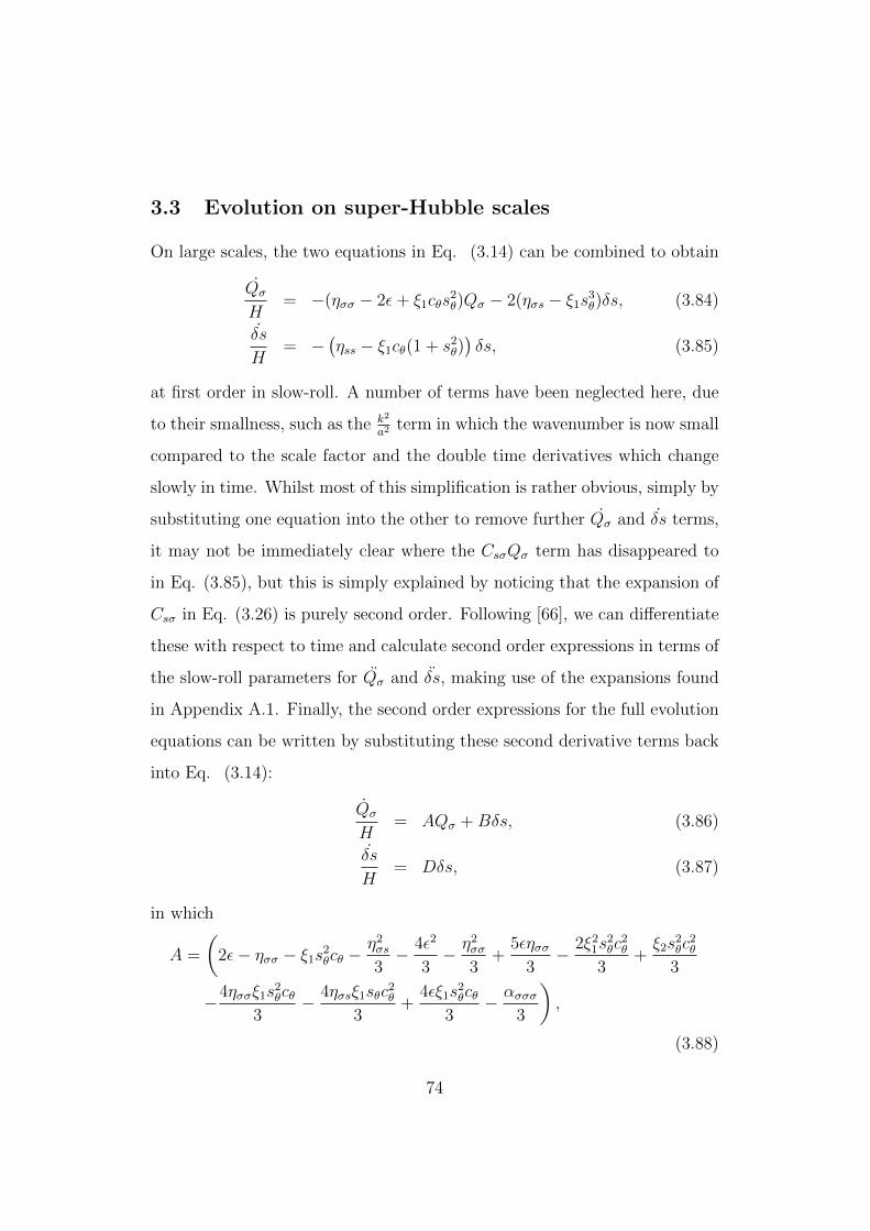
3.3 Evolution on super-Hubble scales

On large scales, the two equations in Eq. (3.14) can be combined to obtain

Qσ

H= −(ησσ − 2ε+ ξ1cθs

2θ)Qσ − 2(ησs − ξ1s

3θ)δs, (3.84)

δs

H= −

(ηss − ξ1cθ(1 + s2

θ))δs, (3.85)

at first order in slow-roll. A number of terms have been neglected here, due

to their smallness, such as the k2

a2 term in which the wavenumber is now small

compared to the scale factor and the double time derivatives which change

slowly in time. Whilst most of this simplification is rather obvious, simply by

substituting one equation into the other to remove further Qσ and δs terms,

it may not be immediately clear where the CsσQσ term has disappeared to

in Eq. (3.85), but this is simply explained by noticing that the expansion of

Csσ in Eq. (3.26) is purely second order. Following [66], we can differentiate

these with respect to time and calculate second order expressions in terms of

the slow-roll parameters for Qσ and δs, making use of the expansions found

in Appendix A.1. Finally, the second order expressions for the full evolution

equations can be written by substituting these second derivative terms back

into Eq. (3.14):

Qσ

H= AQσ +Bδs, (3.86)

δs

H= Dδs, (3.87)

in which

A =

(2ε− ησσ − ξ1s

2θcθ −

η2σs

3− 4ε2

3− η2

σσ

3+

5εησσ3− 2ξ2

1s2θc

2θ

3+ξ2s

2θc

2θ

3

−4ησσξ1s2θcθ

3− 4ησsξ1sθc

2θ

3+

4εξ1s2θcθ

3− ασσσ

3

),

(3.88)

74

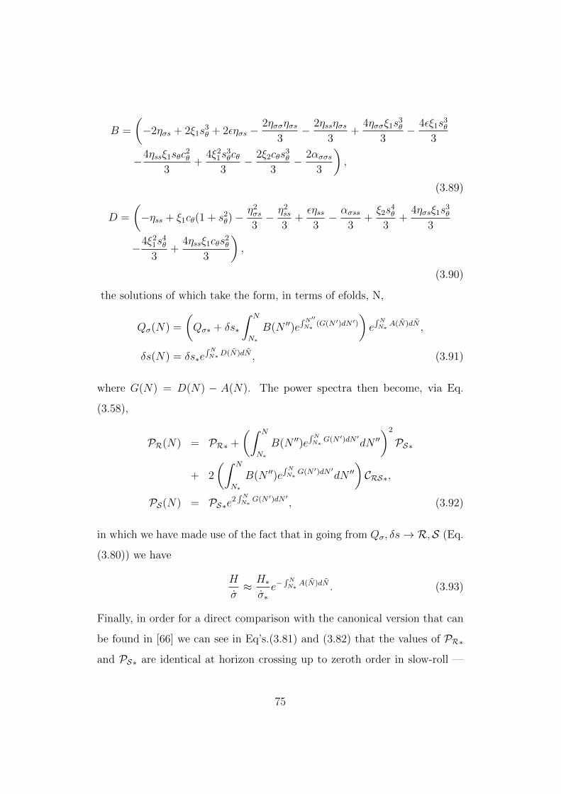
B =

(−2ησs + 2ξ1s

3θ + 2εησs −

2ησσησs3

− 2ηssησs3

+4ησσξ1s

3θ

3− 4εξ1s

3θ

3

−4ηssξ1sθc2θ

3+

4ξ21s

3θcθ

3− 2ξ2cθs

3θ

3− 2ασσs

3

),

(3.89)

D =

(−ηss + ξ1cθ(1 + s2

θ)−η2σs

3− η2

ss

3+εηss3− ασss

3+ξ2s

4θ

3+

4ησsξ1s3θ

3

−4ξ21s

4θ

3+

4ηssξ1cθs2θ

3

),

(3.90)

the solutions of which take the form, in terms of efolds, N,

Qσ(N) =

(Qσ∗ + δs∗

∫ N

N∗

B(N ′′)e∫N′′N∗ (G(N ′)dN ′)

)e∫NN∗ A(N)dN ,

δs(N) = δs∗e∫NN∗D(N)dN , (3.91)

where G(N) = D(N) − A(N). The power spectra then become, via Eq.

(3.58),

PR(N) = PR∗ +

(∫ N

N∗

B(N ′′)e∫NN∗ G(N ′)dN ′dN ′′

)2

PS∗

+ 2

(∫ N

N∗

B(N ′′)e∫NN∗ G(N ′)dN ′dN ′′

)CRS∗,

PS(N) = PS∗e2∫NN∗ G(N ′)dN ′ , (3.92)

in which we have made use of the fact that in going from Qσ, δs→ R,S (Eq.

(3.80)) we have

H

σ≈ H∗

σ∗e−

∫NN∗ A(N)dN . (3.93)

Finally, in order for a direct comparison with the canonical version that can

be found in [66] we can see in Eq’s.(3.81) and (3.82) that the values of PR∗and PS∗ are identical at horizon crossing up to zeroth order in slow-roll —

75

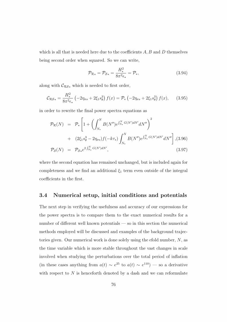
which is all that is needed here due to the coefficients A,B and D themselves

being second order when squared. So we can write,

PR∗ = PS∗ =H2∗

8π2ε∗= P∗, (3.94)

along with CRS∗ which is needed to first order,

CRS∗ =H2∗

8π2ε∗

(−2ησs + 2ξ1s

3θ

)f(x) = P∗

(−2ησs + 2ξ1s

3θ

)f(x), (3.95)

in order to rewrite the final power spectra equations as

PR(N) = P∗

[1 +

(∫ N

N∗

B(N ′′)e∫NN∗ G(N ′)dN ′dN ′′

)2

+ (2ξ1s3θ − 2ησs)f(−kτ∗)

∫ N

N∗

B(N ′′)e∫NN∗ G(N ′)dN ′dN ′′

],(3.96)

PS(N) = PS∗e2∫NN∗ G(N ′)dN ′ , (3.97)

where the second equation has remained unchanged, but is included again for

completeness and we find an additional ξ1 term even outside of the integral

coefficients in the first.

3.4 Numerical setup, initial conditions and potentials

The next step in verifying the usefulness and accuracy of our expressions for

the power spectra is to compare them to the exact numerical results for a

number of different well known potentials — so in this section the numerical

methods employed will be discussed and examples of the background trajec-

tories given. Our numerical work is done solely using the efold number, N , as

the time variable which is more stable throughout the vast changes in scale

involved when studying the perturbations over the total period of inflation

(in these cases anything from a(t) ∼ e25 to a(t) ∼ e110) — so a derivative

with respect to N is henceforth denoted by a dash and we can reformulate

76

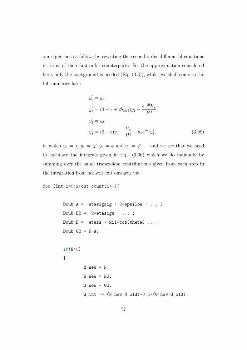
our equations as follows by rewriting the second order differential equations

in terms of their first order counterparts. For the approximation considered

here, only the background is needed (Eq. (3.3)), whilst we shall come to the

full numerics later,

y′0 = y1,

y′1 = (3− ε+ 2bφy3)y1 −e−2bVχH2

,

y′2 = y3,

y′3 = (3− ε)y3 −VφH2

+ bφe2bφy2

1, (3.98)

in which y0 = χ, y1 = χ′, y2 = φ and y3 = φ′ — and we see that we need

to calculate the integrals given in Eq. (3.96) which we do manually by

summing over the small trapezoidal contributions given from each step in

the integration from horizon exit onwards via

for (Int i=0;i<out.count;i++)

Doub A = -etasigsig + 2*epsilon + ... ;

Doub B2 = -2*etasigs + ... ;

Doub D = -etass + xi1*cos(theta) ... ;

Doub G2 = D-A;

if(N>0)

N_new = N;

B_new = B2;

G_new = G2;

G_int += (N_new-N_old)*0.5*(G_new+G_old);

77

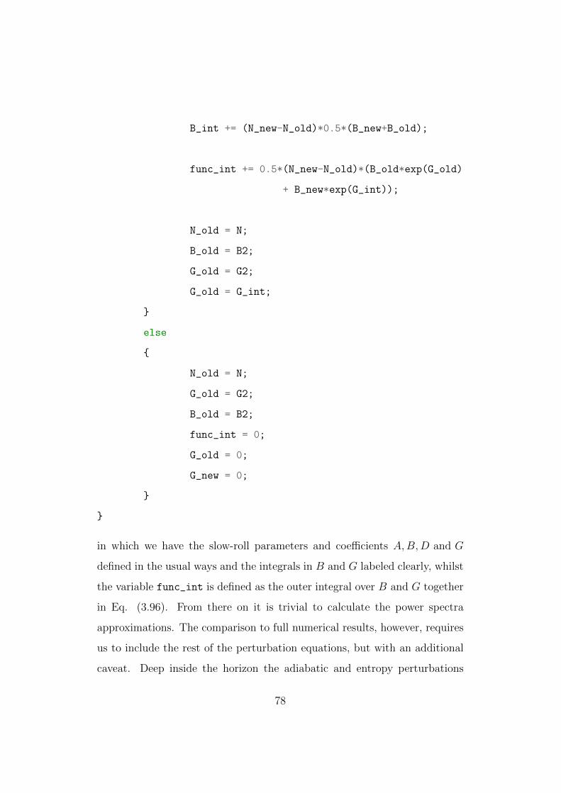
B_int += (N_new-N_old)*0.5*(B_new+B_old);

func_int += 0.5*(N_new-N_old)*(B_old*exp(G_old)

+ B_new*exp(G_int));

N_old = N;

B_old = B2;

G_old = G2;

G_old = G_int;

else

N_old = N;

G_old = G2;

B_old = B2;

func_int = 0;

G_old = 0;

G_new = 0;

in which we have the slow-roll parameters and coefficients A,B,D and G

defined in the usual ways and the integrals in B and G labeled clearly, whilst

the variable func_int is defined as the outer integral over B and G together

in Eq. (3.96). From there on it is trivial to calculate the power spectra

approximations. The comparison to full numerical results, however, requires

us to include the rest of the perturbation equations, but with an additional

caveat. Deep inside the horizon the adiabatic and entropy perturbations

78

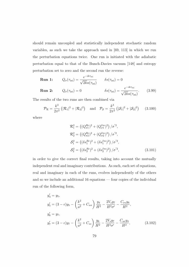
should remain uncoupled and statistically independent stochastic random

variables, as such we take the approach used in [69, 113] in which we run

the perturbation equations twice. One run is initiated with the adiabatic

perturbation equal to that of the Bunch-Davies vacuum [148] and entropy

perturbation set to zero and the second run the reverse:

Run 1: Qσ(τini) =e−ikτini

√2ka(τini)

δs(τini) = 0

Run 2: Qσ(τini) = 0 δs(τini) =e−ikτini

√2ka(τini)

. (3.99)

The results of the two runs are then combined via

PR =k3

2π2

(|R1|2 + |R2|2

)and PS =

k3

2π2

(|S1|2 + |S2|2

)(3.100)

where

R21 =

((QRe

σ1 )2 + (QImσ1 )2

)/σ′2,

R22 =

((QRe

σ2 )2 + (QImσ2 )2

)/σ′2,

S21 =

((δsRe1 )2 + (δsIm1 )2

)/σ′2,

S22 =

((δsRe2 )2 + (δsIm2 )2

)/σ′2, (3.101)

in order to give the correct final results, taking into account the mutually

independent real and imaginary contributions. As such, each set of equations,

real and imaginary in each of the runs, evolves independently of the others

and so we include an additional 16 equations — four copies of the individual

run of the following form,

y′4 = y5,

y′5 = (3− ε)y5 −(k2

a2+ Cσσ

)y4

H2− 2Vsy7

H2σ′− Cσsy6

H2,

y′6 = y7,

y′7 = (3− ε)y7 −(k2

a2+ Css

)y6

H2− 2Vsy7

H2σ′− Csσy4

H2, (3.102)

79

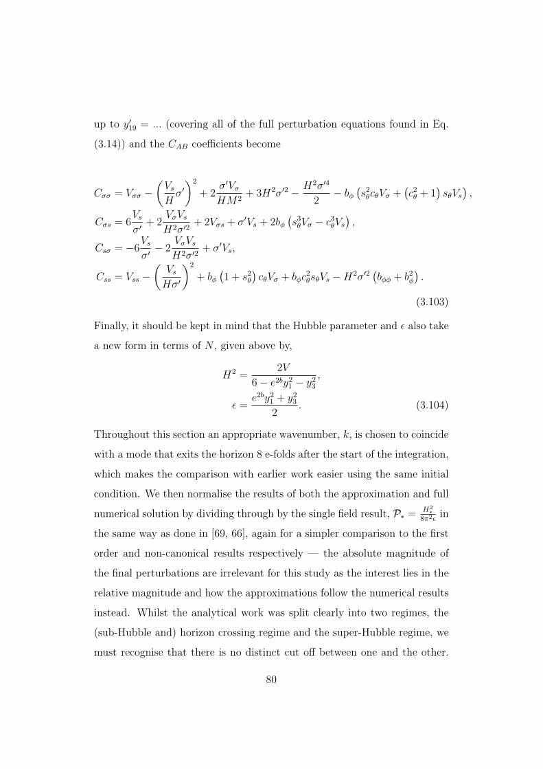
up to y′19 = ... (covering all of the full perturbation equations found in Eq.

(3.14)) and the CAB coefficients become

Cσσ = Vσσ −(VsHσ′)2

+ 2σ′VσHM2

+ 3H2σ′2 − H2σ′4

2− bφ

(s2θcθVσ +

(c2θ + 1

)sθVs

),

Cσs = 6Vsσ′

+ 2VσVsH2σ′2

+ 2Vσs + σ′Vs + 2bφ(s3θVσ − c3

θVs),

Csσ = −6Vsσ′− 2

VσVsH2σ′2

+ σ′Vs,

Css = Vss −(VsHσ′

)2

+ bφ(1 + s2

θ

)cθVσ + bφc

2θsθVs −H2σ′2

(bφφ + b2

φ

).

(3.103)

Finally, it should be kept in mind that the Hubble parameter and ε also take

a new form in terms of N , given above by,

H2 =2V

6− e2by21 − y2

3

,

ε =e2by2

1 + y23

2. (3.104)

Throughout this section an appropriate wavenumber, k, is chosen to coincide

with a mode that exits the horizon 8 e-folds after the start of the integration,

which makes the comparison with earlier work easier using the same initial

condition. We then normalise the results of both the approximation and full

numerical solution by dividing through by the single field result, P∗ = H2∗

8π2εin

the same way as done in [69, 66], again for a simpler comparison to the first

order and non-canonical results respectively — the absolute magnitude of

the final perturbations are irrelevant for this study as the interest lies in the

relative magnitude and how the approximations follow the numerical results

instead. Whilst the analytical work was split clearly into two regimes, the

(sub-Hubble and) horizon crossing regime and the super-Hubble regime, we

must recognise that there is no distinct cut off between one and the other.

80

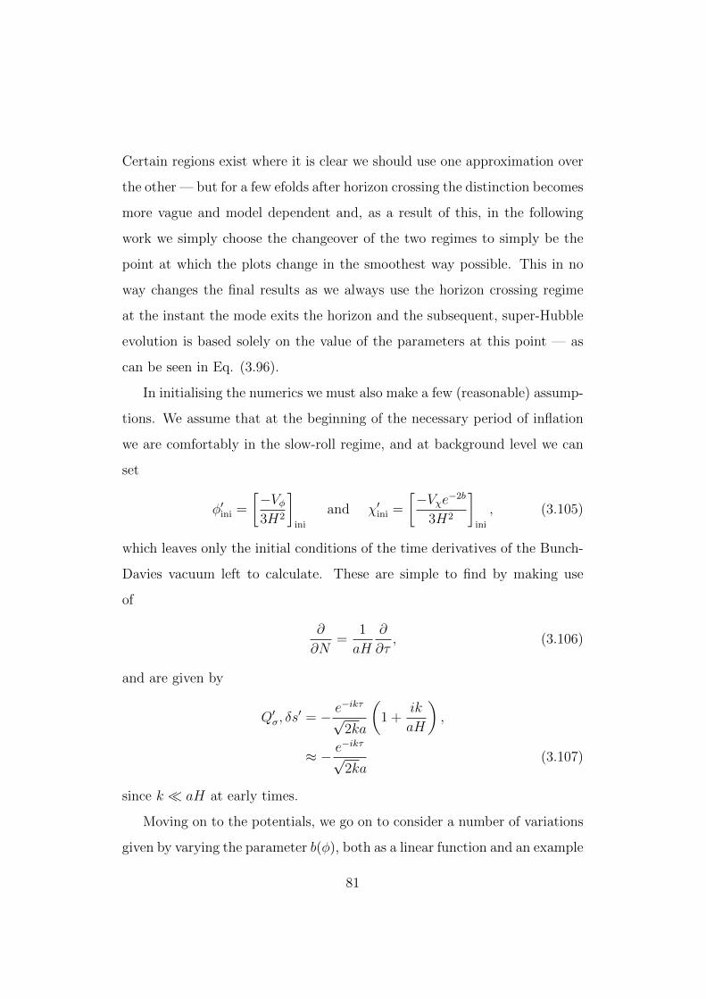
Certain regions exist where it is clear we should use one approximation over

the other — but for a few efolds after horizon crossing the distinction becomes

more vague and model dependent and, as a result of this, in the following

work we simply choose the changeover of the two regimes to simply be the

point at which the plots change in the smoothest way possible. This in no

way changes the final results as we always use the horizon crossing regime

at the instant the mode exits the horizon and the subsequent, super-Hubble

evolution is based solely on the value of the parameters at this point — as

can be seen in Eq. (3.96).

In initialising the numerics we must also make a few (reasonable) assump-

tions. We assume that at the beginning of the necessary period of inflation

we are comfortably in the slow-roll regime, and at background level we can

set

φ′ini =

[−Vφ3H2

]ini

and χ′ini =

[−Vχe−2b

3H2

]ini

, (3.105)

which leaves only the initial conditions of the time derivatives of the Bunch-

Davies vacuum left to calculate. These are simple to find by making use

of

∂

∂N=

1

aH

∂

∂τ, (3.106)

and are given by

Q′σ, δs′ = − e

−ikτ√

2ka

(1 +

ik

aH

),

≈ − e−ikτ√

2ka(3.107)

since k aH at early times.

Moving on to the potentials, we go on to consider a number of variations

given by varying the parameter b(φ), both as a linear function and an example

81

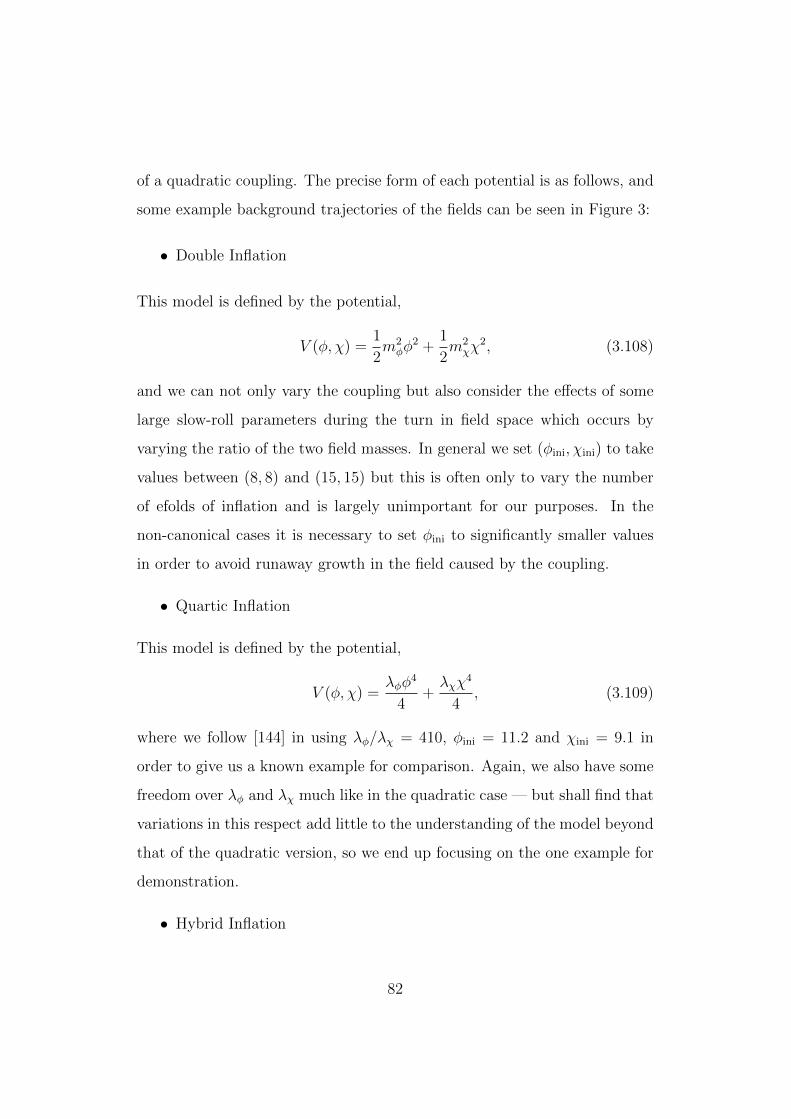
of a quadratic coupling. The precise form of each potential is as follows, and

some example background trajectories of the fields can be seen in Figure 3:

• Double Inflation

This model is defined by the potential,

V (φ, χ) =1

2m2φφ

2 +1

2m2χχ

2, (3.108)

and we can not only vary the coupling but also consider the effects of some

large slow-roll parameters during the turn in field space which occurs by

varying the ratio of the two field masses. In general we set (φini, χini) to take

values between (8, 8) and (15, 15) but this is often only to vary the number

of efolds of inflation and is largely unimportant for our purposes. In the

non-canonical cases it is necessary to set φini to significantly smaller values

in order to avoid runaway growth in the field caused by the coupling.

• Quartic Inflation

This model is defined by the potential,

V (φ, χ) =λφφ

4

4+λχχ

4

4, (3.109)

where we follow [144] in using λφ/λχ = 410, φini = 11.2 and χini = 9.1 in

order to give us a known example for comparison. Again, we also have some

freedom over λφ and λχ much like in the quadratic case — but shall find that

variations in this respect add little to the understanding of the model beyond

that of the quadratic version, so we end up focusing on the one example for

demonstration.

• Hybrid Inflation

82

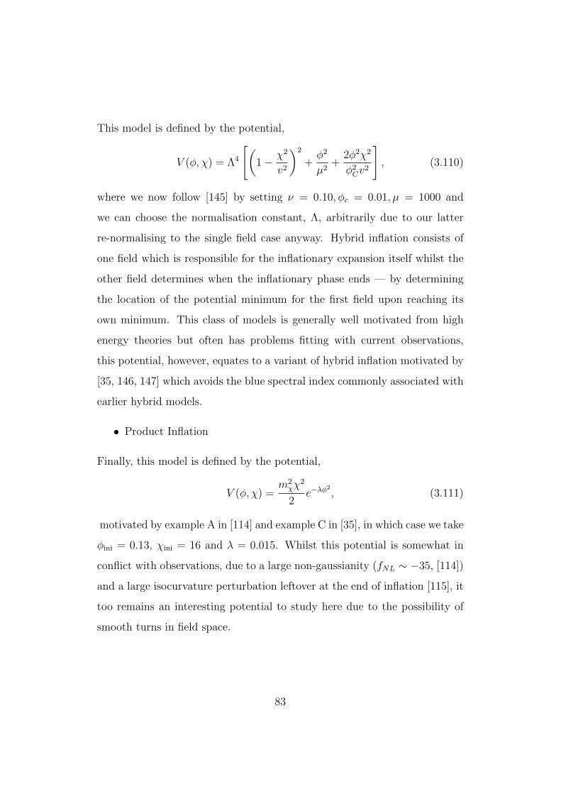
This model is defined by the potential,

V (φ, χ) = Λ4

[(1− χ2

v2

)2

+φ2

µ2+

2φ2χ2

φ2Cv

2

], (3.110)

where we now follow [145] by setting ν = 0.10, φc = 0.01, µ = 1000 and

we can choose the normalisation constant, Λ, arbitrarily due to our latter

re-normalising to the single field case anyway. Hybrid inflation consists of

one field which is responsible for the inflationary expansion itself whilst the

other field determines when the inflationary phase ends — by determining

the location of the potential minimum for the first field upon reaching its

own minimum. This class of models is generally well motivated from high

energy theories but often has problems fitting with current observations,

this potential, however, equates to a variant of hybrid inflation motivated by

[35, 146, 147] which avoids the blue spectral index commonly associated with

earlier hybrid models.

• Product Inflation

Finally, this model is defined by the potential,

V (φ, χ) =m2χχ

2

2e−λφ

2

, (3.111)

motivated by example A in [114] and example C in [35], in which case we take

φini = 0.13, χini = 16 and λ = 0.015. Whilst this potential is somewhat in

conflict with observations, due to a large non-gaussianity (fNL ∼ −35, [114])

and a large isocurvature perturbation leftover at the end of inflation [115], it

too remains an interesting potential to study here due to the possibility of

smooth turns in field space.

83

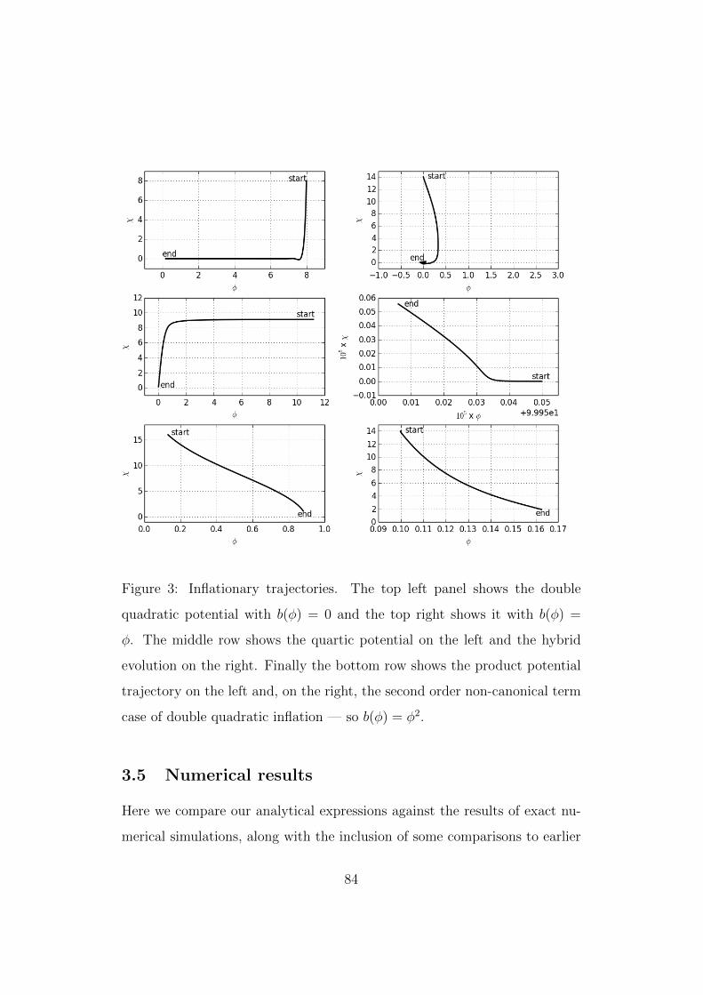
Figure 3: Inflationary trajectories. The top left panel shows the double

quadratic potential with b(φ) = 0 and the top right shows it with b(φ) =

φ. The middle row shows the quartic potential on the left and the hybrid

evolution on the right. Finally the bottom row shows the product potential

trajectory on the left and, on the right, the second order non-canonical term

case of double quadratic inflation — so b(φ) = φ2.

3.5 Numerical results

Here we compare our analytical expressions against the results of exact nu-

merical simulations, along with the inclusion of some comparisons to earlier

84

work such as that of [66] and [69]. Following convention, we choose N such

that the zeroth efold is associated with the time that the mode of interest

crosses the horizon — with sub-horizon evolution denoted by negative values.

3.5.1 Double Inflation

b(φ) = 0

Looking initially at the case of b(φ) = 0, which leaves us with the usual

canonical case, we can see that the top left graph in Figure 3 shows inflation

begins with the χ field dominating proceedings before a sharp turn in field

space allows the φ field to subsequently take over. During these two separate

phases — in which one field dominates over the other — there are few inter-

esting effects because the isocurvature perturbations are small. During the

transition period, however, the isocurvature perturbations and, more impor-

tantly, the sourcing by these of curvature perturbations is greatly enhanced,

which leads to the large increase in PR that is seen in Figure 4. In agreement

with [66], we find that our second order approximation captures this well for

field mass ratios up to mχmφ∼ 9, with the example shown in Figure 4 (using

mχmφ∼ 7) showing a perfect match. Beyond this ratio, however, as the turn

in field space gets ever sharper, we start to see higher order effects playing

a role as the subsequent ‘wobbles’ about the valley bottom in field space

allow numerous additional opportunities for the curvature perturbation to

be further enhanced. In Figure 5 this is demonstrated as a mass ratio of

mχmφ

= 10 is used to show that the final power spectrum is severely under-

estimated (whilst still being a significant improvement over the first order

version) in comparison to the full numerical result. It should also be noted

that the isocurvature perturbations are similarly inaccurate in this case, but

the qualitative behaviour remains well approximated.

85

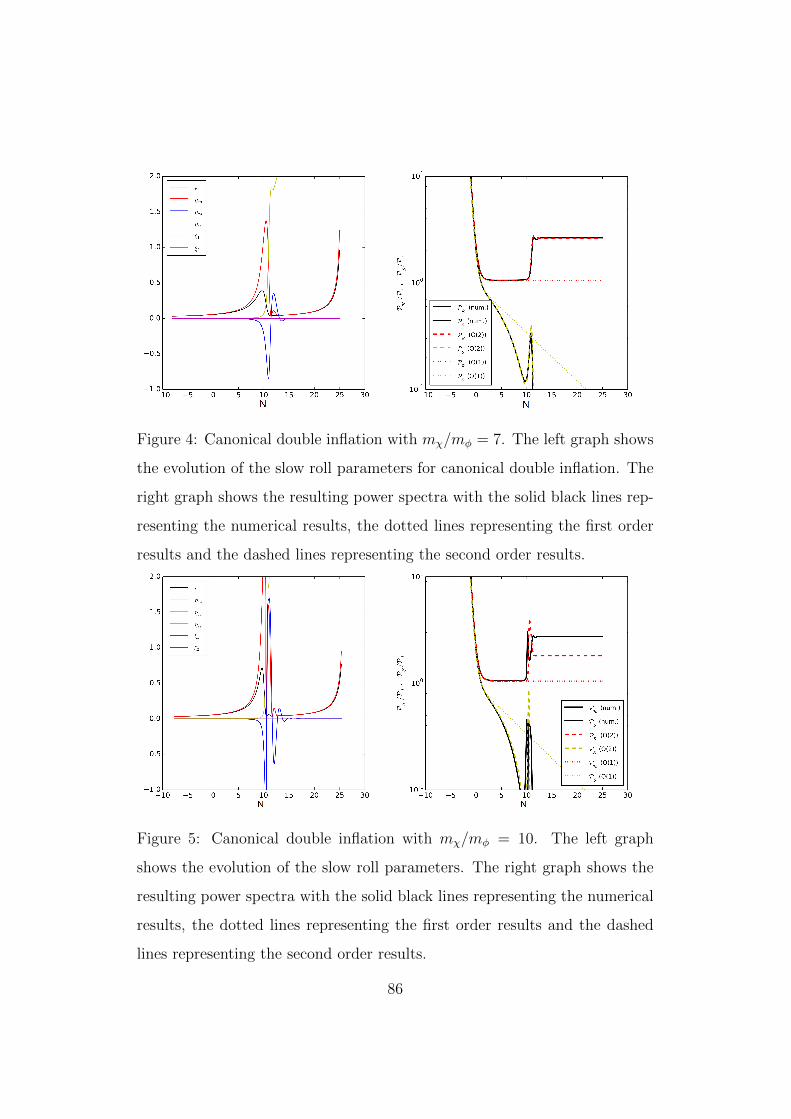
Figure 4: Canonical double inflation with mχ/mφ = 7. The left graph shows

the evolution of the slow roll parameters for canonical double inflation. The

right graph shows the resulting power spectra with the solid black lines rep-

resenting the numerical results, the dotted lines representing the first order

results and the dashed lines representing the second order results.

Figure 5: Canonical double inflation with mχ/mφ = 10. The left graph

shows the evolution of the slow roll parameters. The right graph shows the

resulting power spectra with the solid black lines representing the numerical

results, the dotted lines representing the first order results and the dashed

lines representing the second order results.

86

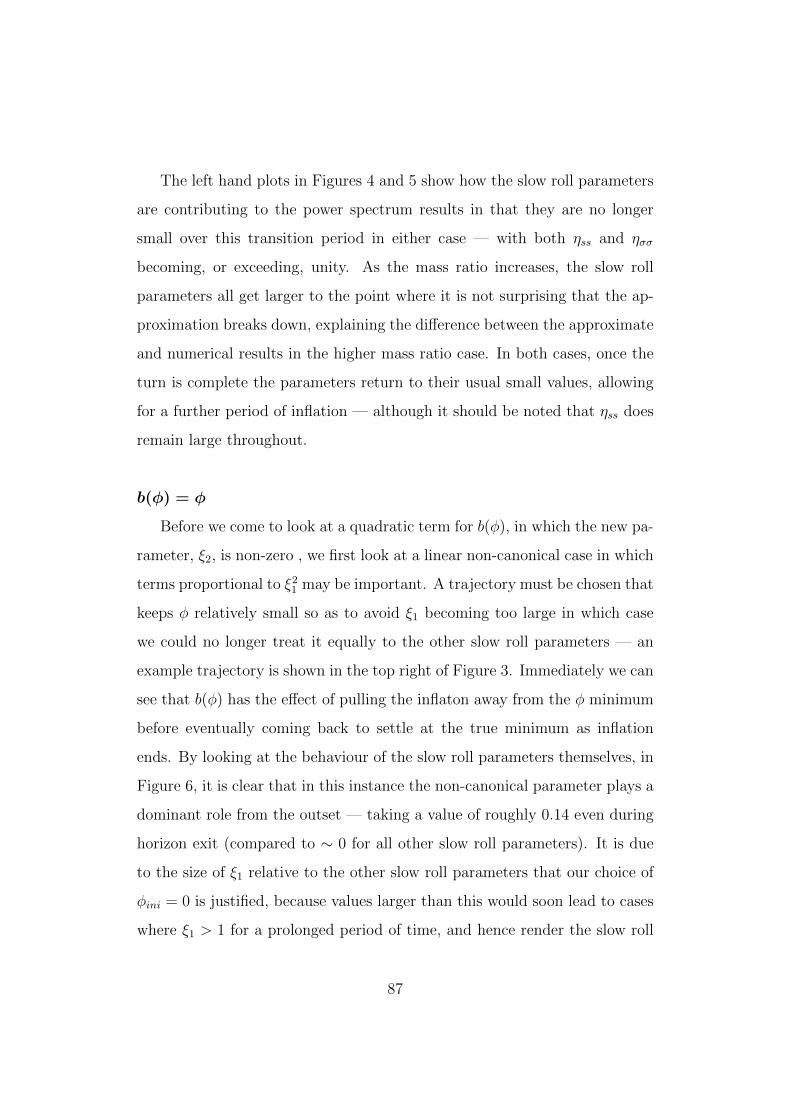
The left hand plots in Figures 4 and 5 show how the slow roll parameters

are contributing to the power spectrum results in that they are no longer

small over this transition period in either case — with both ηss and ησσ

becoming, or exceeding, unity. As the mass ratio increases, the slow roll

parameters all get larger to the point where it is not surprising that the ap-

proximation breaks down, explaining the difference between the approximate

and numerical results in the higher mass ratio case. In both cases, once the

turn is complete the parameters return to their usual small values, allowing

for a further period of inflation — although it should be noted that ηss does

remain large throughout.

b(φ) = φ

Before we come to look at a quadratic term for b(φ), in which the new pa-

rameter, ξ2, is non-zero , we first look at a linear non-canonical case in which

terms proportional to ξ21 may be important. A trajectory must be chosen that

keeps φ relatively small so as to avoid ξ1 becoming too large in which case

we could no longer treat it equally to the other slow roll parameters — an

example trajectory is shown in the top right of Figure 3. Immediately we can

see that b(φ) has the effect of pulling the inflaton away from the φ minimum

before eventually coming back to settle at the true minimum as inflation

ends. By looking at the behaviour of the slow roll parameters themselves, in

Figure 6, it is clear that in this instance the non-canonical parameter plays a

dominant role from the outset — taking a value of roughly 0.14 even during

horizon exit (compared to ∼ 0 for all other slow roll parameters). It is due

to the size of ξ1 relative to the other slow roll parameters that our choice of

φini = 0 is justified, because values larger than this would soon lead to cases

where ξ1 > 1 for a prolonged period of time, and hence render the slow roll

87

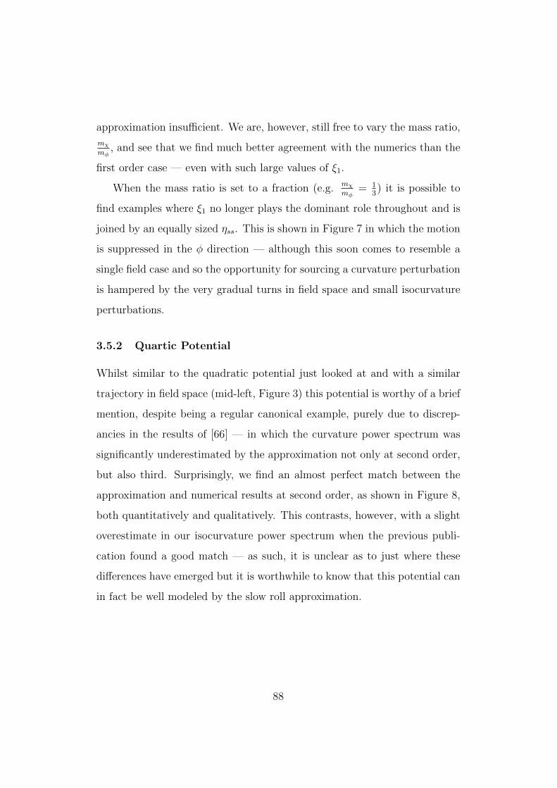
approximation insufficient. We are, however, still free to vary the mass ratio,

mχmφ

, and see that we find much better agreement with the numerics than the

first order case — even with such large values of ξ1.

When the mass ratio is set to a fraction (e.g. mχmφ

= 13) it is possible to

find examples where ξ1 no longer plays the dominant role throughout and is

joined by an equally sized ηss. This is shown in Figure 7 in which the motion

is suppressed in the φ direction — although this soon comes to resemble a

single field case and so the opportunity for sourcing a curvature perturbation

is hampered by the very gradual turns in field space and small isocurvature

perturbations.

3.5.2 Quartic Potential

Whilst similar to the quadratic potential just looked at and with a similar

trajectory in field space (mid-left, Figure 3) this potential is worthy of a brief

mention, despite being a regular canonical example, purely due to discrep-

ancies in the results of [66] — in which the curvature power spectrum was

significantly underestimated by the approximation not only at second order,

but also third. Surprisingly, we find an almost perfect match between the

approximation and numerical results at second order, as shown in Figure 8,

both quantitatively and qualitatively. This contrasts, however, with a slight

overestimate in our isocurvature power spectrum when the previous publi-

cation found a good match — as such, it is unclear as to just where these

differences have emerged but it is worthwhile to know that this potential can

in fact be well modeled by the slow roll approximation.

88

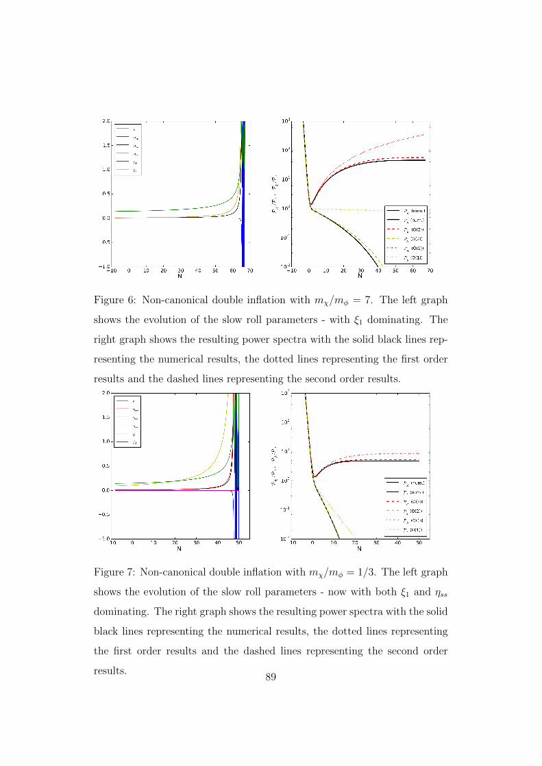
Figure 6: Non-canonical double inflation with mχ/mφ = 7. The left graph

shows the evolution of the slow roll parameters - with ξ1 dominating. The

right graph shows the resulting power spectra with the solid black lines rep-

resenting the numerical results, the dotted lines representing the first order

results and the dashed lines representing the second order results.

Figure 7: Non-canonical double inflation with mχ/mφ = 1/3. The left graph

shows the evolution of the slow roll parameters - now with both ξ1 and ηss

dominating. The right graph shows the resulting power spectra with the solid

black lines representing the numerical results, the dotted lines representing

the first order results and the dashed lines representing the second order

results.89

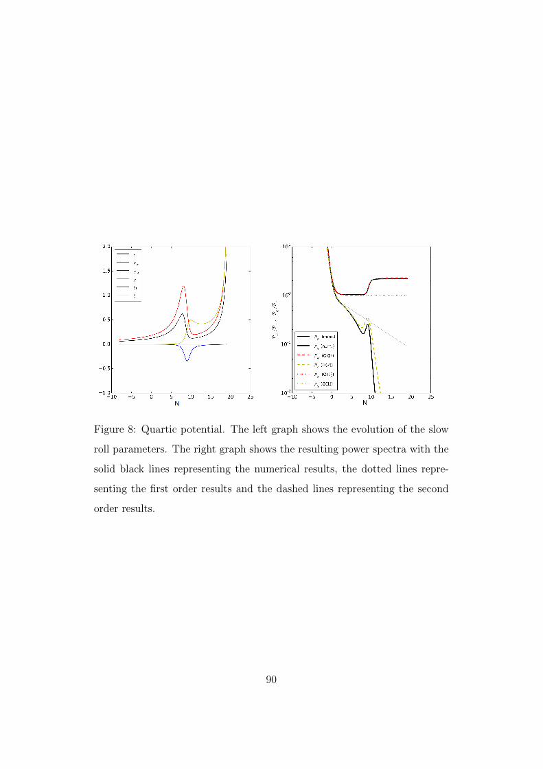
Figure 8: Quartic potential. The left graph shows the evolution of the slow

roll parameters. The right graph shows the resulting power spectra with the

solid black lines representing the numerical results, the dotted lines repre-

senting the first order results and the dashed lines representing the second

order results.

90

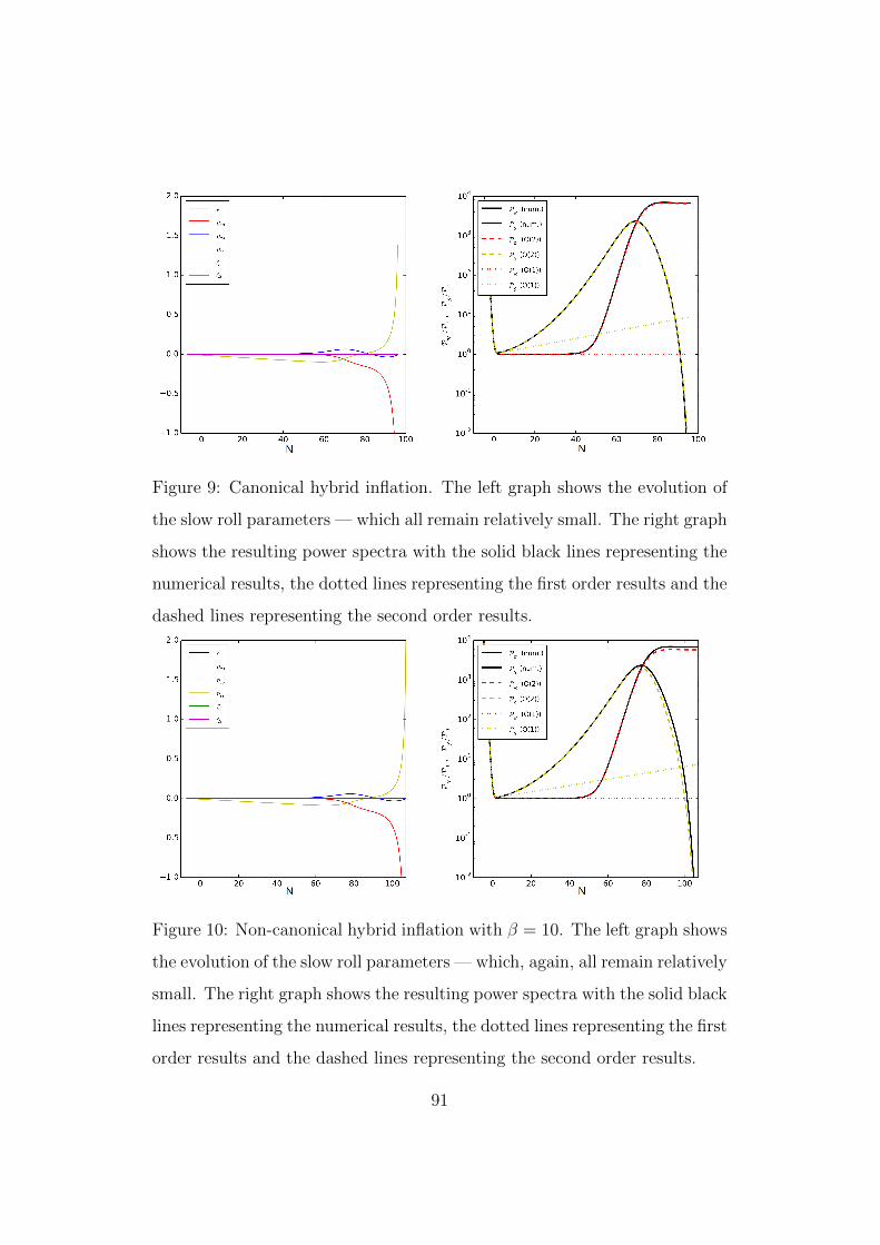
Figure 9: Canonical hybrid inflation. The left graph shows the evolution of

the slow roll parameters — which all remain relatively small. The right graph

shows the resulting power spectra with the solid black lines representing the

numerical results, the dotted lines representing the first order results and the

dashed lines representing the second order results.

Figure 10: Non-canonical hybrid inflation with β = 10. The left graph shows

the evolution of the slow roll parameters — which, again, all remain relatively

small. The right graph shows the resulting power spectra with the solid black

lines representing the numerical results, the dotted lines representing the first

order results and the dashed lines representing the second order results.

91

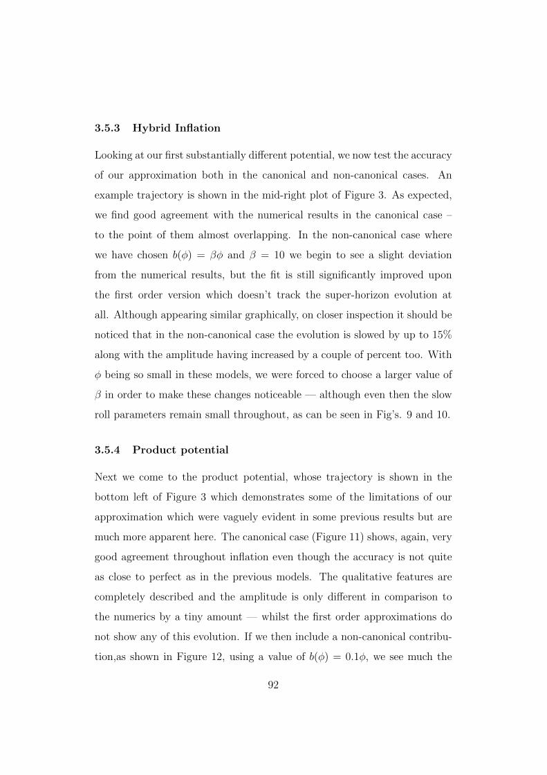
3.5.3 Hybrid Inflation

Looking at our first substantially different potential, we now test the accuracy

of our approximation both in the canonical and non-canonical cases. An

example trajectory is shown in the mid-right plot of Figure 3. As expected,

we find good agreement with the numerical results in the canonical case –

to the point of them almost overlapping. In the non-canonical case where

we have chosen b(φ) = βφ and β = 10 we begin to see a slight deviation

from the numerical results, but the fit is still significantly improved upon

the first order version which doesn’t track the super-horizon evolution at

all. Although appearing similar graphically, on closer inspection it should be

noticed that in the non-canonical case the evolution is slowed by up to 15%

along with the amplitude having increased by a couple of percent too. With

φ being so small in these models, we were forced to choose a larger value of

β in order to make these changes noticeable — although even then the slow

roll parameters remain small throughout, as can be seen in Fig’s. 9 and 10.

3.5.4 Product potential

Next we come to the product potential, whose trajectory is shown in the

bottom left of Figure 3 which demonstrates some of the limitations of our

approximation which were vaguely evident in some previous results but are

much more apparent here. The canonical case (Figure 11) shows, again, very

good agreement throughout inflation even though the accuracy is not quite

as close to perfect as in the previous models. The qualitative features are

completely described and the amplitude is only different in comparison to

the numerics by a tiny amount — whilst the first order approximations do

not show any of this evolution. If we then include a non-canonical contribu-

tion,as shown in Figure 12, using a value of b(φ) = 0.1φ, we see much the

92

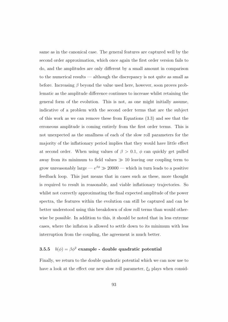
same as in the canonical case. The general features are captured well by the

second order approximation, which once again the first order version fails to

do, and the amplitudes are only different by a small amount in comparison

to the numerical results — although the discrepancy is not quite as small as

before. Increasing β beyond the value used here, however, soon proves prob-

lematic as the amplitude difference continues to increase whilst retaining the

general form of the evolution. This is not, as one might initially assume,

indicative of a problem with the second order terms that are the subject

of this work as we can remove these from Equations (3.3) and see that the

erroneous amplitude is coming entirely from the first order terms. This is

not unexpected as the smallness of each of the slow roll parameters for the

majority of the inflationary period implies that they would have little effect

at second order. When using values of β > 0.1, φ can quickly get pulled

away from its minimum to field values 10 leaving our coupling term to

grow unreasonably large — eβφ 20000 — which in turn leads to a positive

feedback loop. This just means that in cases such as these, more thought

is required to result in reasonable, and viable inflationary trajectories. So

whilst not correctly approximating the final expected amplitude of the power

spectra, the features within the evolution can still be captured and can be

better understood using this breakdown of slow roll terms than would other-

wise be possible. In addition to this, it should be noted that in less extreme

cases, where the inflaton is allowed to settle down to its minimum with less

interruption from the coupling, the agreement is much better.

3.5.5 b(φ) = βφ2 example - double quadratic potential

Finally, we return to the double quadratic potential which we can now use to

have a look at the effect our new slow roll parameter, ξ2 plays when consid-

93

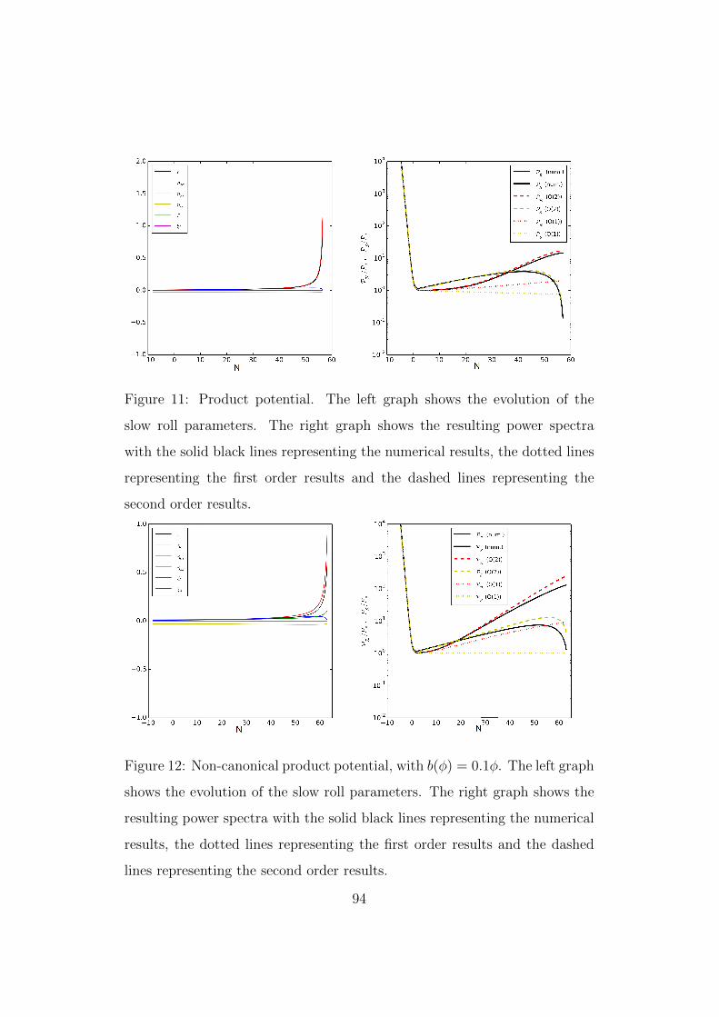
Figure 11: Product potential. The left graph shows the evolution of the

slow roll parameters. The right graph shows the resulting power spectra

with the solid black lines representing the numerical results, the dotted lines

representing the first order results and the dashed lines representing the

second order results.

Figure 12: Non-canonical product potential, with b(φ) = 0.1φ. The left graph

shows the evolution of the slow roll parameters. The right graph shows the

resulting power spectra with the solid black lines representing the numerical

results, the dotted lines representing the first order results and the dashed

lines representing the second order results.

94

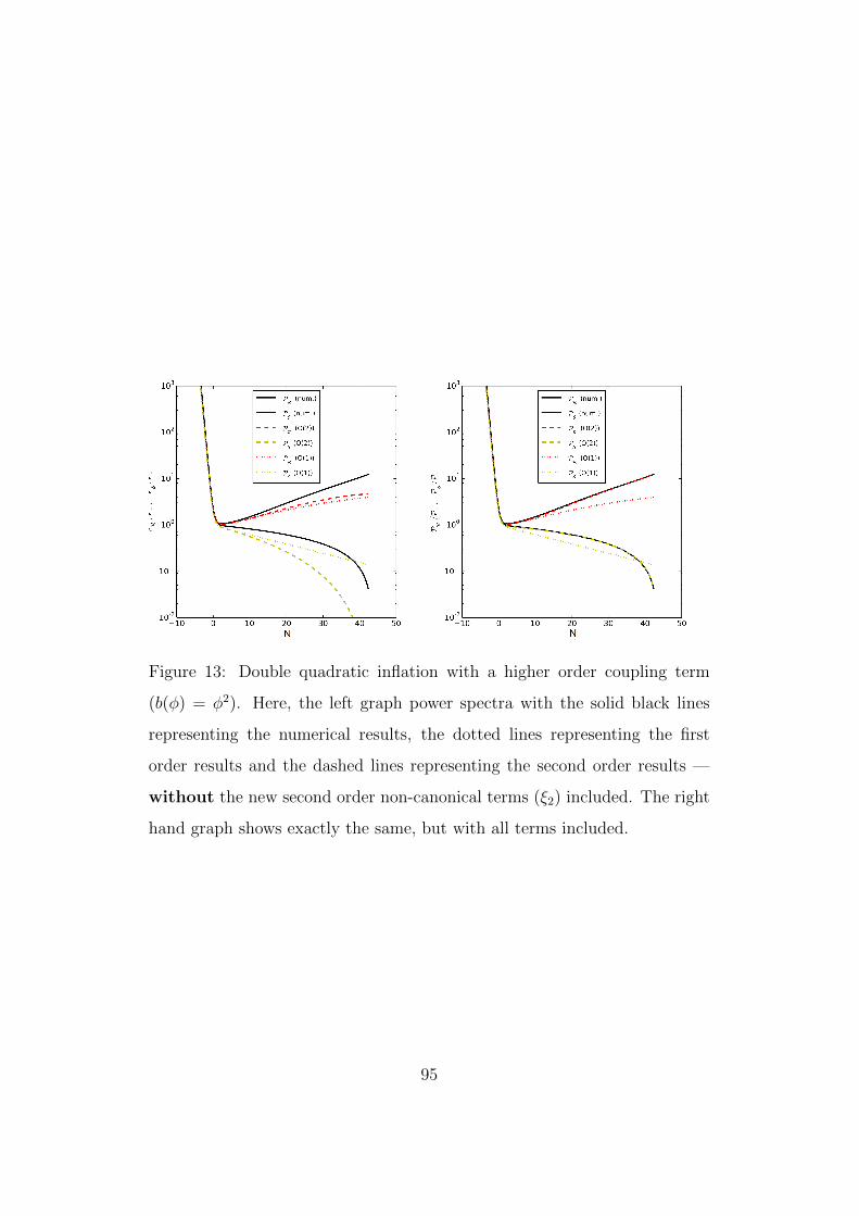
Figure 13: Double quadratic inflation with a higher order coupling term

(b(φ) = φ2). Here, the left graph power spectra with the solid black lines

representing the numerical results, the dotted lines representing the first

order results and the dashed lines representing the second order results —

without the new second order non-canonical terms (ξ2) included. The right

hand graph shows exactly the same, but with all terms included.

95

ering higher powers of φ in b(φ). With this form of the coupling, we hoped

to keep the initial conditions and trajectory as similar as possible to the ear-

lier non-canonical case for ease of comparison and with the expectation that

we would find a reasonable inflationary model — with no runaway feedback

loops such as those that were problematic in the previous case. Although,

it was necessary here to pull the initial value of φ away from zero so as to

avoid an effective single field evolution due to the presence of φ in the b(φ)

derivatives in the background equations. The results are plotted in Figure 13

and shows the power spectra from two runs of the same inflationary model.

The left hand plot shows an example in which all of the ξ2 terms have been

removed and so any second order non-canonical contribution is once again

coming solely from terms proportional to ξ21 whilst the right hand plot shows

the full results with their inclusion. It is clear that in the first example the an-

alytical expressions fail to track the power spectra with any sort of accuracy,

but the full results show near-perfect agreement with both the curvature and

isocurvature power spectra — overlapping throughout.

3.6 Conclusions

In this chapter we have considered the effect on the power spectra, both

curvature and isocurvature, of non-canonical kinetic terms of the form eb(φ)

where we have set b(φ) = βφ or b(φ) = βφ2. The latter coupling makes it

necessary to introduce a new parameter which we treat the same as a second

order slow roll parameter, analogously to the first order version introduced

in [69], ξ1. The effects of non-canonical kinetic terms can have important

consequences on the background trajectories and hence the slow roll param-

eters and turns in a multidimensional field space — which in turn directly

affects the final amplitude of the power spectra via the sourcing of the cur-

96

vature perturbation from isocurvature perturbations on super-horizon scales.

Whilst the majority of the cases studied here involve only the linear coupling

and hence leave ξ2 = 0, the final example shows the importance of such terms

and provides a basis for further work in this direction. It has also been shown

that in such cases as the linear coupling, the first order approximation is very

rarely enough to track the evolution of the power spectra — with second or-

der ξ21 terms playing an important role both qualitatively and quantitatively

as ξ1 itself can often dominate over the other slow roll parameters.

Unfortunately, in comparison to the second order approximation of canon-

ical cases, the approximation is sometimes not quite as accurate as might be

hoped, but this slight loss of accuracy should be understood to come not

from the expansion itself, but rather from the need to more carefully choose

inflationary trajectories and be aware of how they are altered by the cou-

pling. For example, taking another look at Figures 11 and 12 the loss in

accuracy here in the non-canonical case comes from the turn in field space

becoming much sharper rather than any unreasonable growth in the non-

canonical slow roll parameters (which both remain 1 for the majority of

inflation) — this altered trajectory leads to changes in the standard slow

roll parameters and, in this instance, an increase in ηss which then provides

the dominant contribution. The fact that the canonical contributions have

been well measured and understood in previous work [66], which agrees with

our expressions, means that we can be confident that in the vast majority of

cases this should not be an issue so long as we remain aware of it.

Finally, it should be emphasised that whilst we find an improvement on

previous approximations through the inclusion of second order non-canonical

terms it it still necessary to artificially constrain the magnitude of b(φ) (either

through careful choice of φini or by keeping β small) in order for the new

97

parameters to be appropriately treated as slow roll parameters and for the

approximation to work.

98

4 Stabilising the Planck mass after

inflation

Having touched upon non-minimal couplings to gravity in the introduction,

we will now look at how such couplings can be used to vary the effective

Planck mass during inflation before allowing it to settle to the current value

after the universe reheats. Current tests of General Relativity have placed

tight constraints on variations in the Planck mass (or, alternatively, the grav-

itational constant) in the recent history of the universe by measuring it on

different scales, using different methods [149], with the current value of G

measured to be 6.67384(50) × 10−11m3kg−1s−2 [150]. It remains to be seen

whether or not it evolved in time in the early universe though — something

which could leave signatures in the curvature perturbation power spectrum

produced by inflation. We allow the Planck mass to vary by allowing a sec-

ondary field — very similar, or in some cases identical, to the curvaton [151]

— to be non-minimally coupled to gravity which then varies throughout infla-

tion, before leading to a secondary decay phase (after the inflaton) in which

the universe finally totally reheats and the power spectrum becomes frozen

in. It is known that rapid oscillations of the fields during the radiation dom-

inated phase can cause changes in the subsequent expansion history of the

universe [152, 153] and it is believed that through the coupling and additional

terms in the non-adiabatic pressure perturbation, it should be possible to see

significant changes during the oscillatory reheating phase of the secondary

field to the primordial power spectrum — a result that could be used to open

up or further constrain various models of inflation [154] and something we

shall investigate here. For clarity as to how the Planck mass is varied by a

non-minimal coupling, one only needs to consider the definition of the Planck

99

mass, MP =√

(hc/G) to see that a varying effective gravitational constant

can result in a varying effective Planck Mass.

4.1 Non-minimally coupled curvaton

The theory we are considering here is specified by the action,

S =

∫d4x√−g[

1

2f(σ)R− 1

2gµν (∂µφ∂νφ+ ∂µσ∂νσ)− V (φ, σ) + Lint

](4.1)

where gµν is the metric tensor, V (φ, σ) the potential of the two scalar fields

— the inflaton, φ, and the curvaton, σ, which we assume are not directly

interacting — and Lint is the interaction Lagrangian used to describe the

perturbative decay [35] of both of the fields into radiation — involving only

a minimal coupling to gravity. By working in the Jordan frame, the decay

rates can be calculated in the standard way and are denoted by Γφ and Γσ for

the two fields respectively. By comparing the form of this action to a more

standard case, for example, Eq. (3.1), we can see that the effective Planck

Mass is now defined as

MP =√f(σ), (4.2)

where, in general, we normalise the final value to be equal to 1 in subsequent

work. Whilst we could in principle admit any form of f(σ) we instead take

a quadratic approximation,

f(σ) = 1 +α

2(σ − σmin)2, (4.3)

which dominates the dynamics — especially using the small values we find

necessary later. The masses of the fields are given by mφ and mσ so that the

potential under consideration takes the form

V (φ, σ) =1

2m2φφ

2 +1

2m2σσ

2. (4.4)

100

The metric takes the usual form,

ds2 = −(1 + 2Φ)dt2 + a2(t) (1− 2Ψ) δijdxidxj, (4.5)

but unlike in the standard case, with the inclusion of the non-minimal cou-

pling, in the Jordan frame, Φ and Ψ are no longer equal even in the absence

of anisotropic stress and the constraint now becomes [86],

Φ = Ψ− δf

f. (4.6)

This is calculated from the off diagonal terms of the stress-energy tensor,

T ij , i 6= j giving,

∂i∂j(Φ−Ψ) = − 1

f∂i∂jδf. (4.7)

The metric perturbation, Ψ, satisfies the following evolution equation

Ψ = −3HΨ−HΦ−H2(3− 2ε)Φ

+1

2f

[φ ˙δφ+ σ ˙δσ − (φ2 + σ2)Φ− Vφδφ− Vσδσ +

δργ3− 2fΦ− f(Ψ + 2HΦ)

−δff

(φ2

2+σ2

2− V + f + 2Hf

)+ δf + 2H ˙δf +

k2

a2δf

], (4.8)

whilst we can also make use of

3H(Ψ +HΦ) +k2

a2Ψ = − 1

2f

[φ ˙δφ+ σ ˙δσ − (φ2 + σ2)Φ + Vφδφ+ Vσδσ + δργ

+ 3f(

Ψ + 2HΦ)− 3H

(˙δf +Hδf

)− k2

a2δf

]Ψ +HΦ = − 1

2f

[φδφ+ σδσ + ˙δf −Hδf

], (4.9)

although these additional equations are superfluous to the calculations. At

this point, we are working again on Fourier modes although the subscript, k,

has been dropped. We can now vary the action to find the modified equations

101

of motion for the system, with the inclusion of the phenomenological decay

terms, as

φ = −Vφ − 3Hφ− Γφφ , (4.10)

σ = −Vσ − 3Hσ +fσR

2− Γσσ , (4.11)

at background level for the fields, along with the energy conservation equation

for the radiation fluid

ργ = −4Hργ + Γφφ2 + Γσσ

2 , (4.12)

and the Friedmann equation

H2 =1

3f

[φ2

2+σ2

2+ V + ργ

]− fσσH

f. (4.13)

We also have that

H = −1

2

(φ2 + σ2 + 2f − 2Hf +

4ργ3

). (4.14)

In this section an overdot continues to signify a derivative with respect to cos-

mic time whilst subscripts signify a derivative with respect to the respective

field. The slow roll parameter, ε, also continues to be defined by [155],

ε ≡ − H

H2, (4.15)

but we see from the above Friedmann equations that there is now an implicit

dependence on f(σ) within it. The Ricci scalar can be succinctly written

using this as

R = 6H2(2− ε), (4.16)

along with its perturbation being given by

δR = −6Ψ− 6H(Φ + 4Ψ)− 2RΦ + 2k2

a2(Φ− 2Ψ) . (4.17)

102

Considering now the linear perturbations, we obtain a Klein-Gordon

equation for each field [86]

δφ = −(3H + Γφ) ˙δφ−(k2

a2+ Vφφ

)δφ− Vφσδσ + φ(Φ + 3Ψ)− (2Vφ + Γφφ)Φ ,

(4.18)

δσ = −(3H + Γσ) ˙δσ −(k2

a2+ Vσσ −

fσσR

2

)δσ − Vσφδφ+ σ(Φ + 3Ψ)

− (2Vσ + Γσσ)Φ +fσ2

(2RΦ + δR) ,

(4.19)

along with a first order conservation equation for the radiation fluid

˙δργ = −4Hδργ+4HργΦ−2k2

a2(Ψ+HΦ)+2Γφ(φ ˙δφ+

φ2

2Φ)+2Γσ(σ ˙δσ+

σ2

2Φ) .

(4.20)

It may not be immediately obvious as to how the terms including the decay

rates in the last equation take the given form, so as a short aside we shall

take a look at the derivation. Beginning with

∇µTµν = 0 = ∂µT

µν + ΓµµαT

αν − ΓαµνT

µα , (4.21)

in the standard case (without source terms), noting that ΓABC used here refers

to the Christoffel symbols rather than the decay rates denoted by ΓA. For

ν = 0 we have

∂0T00 + ∂iT

i0 + Γµµ0T

00 + Γ0

00T00 − Γij0T

ij = 0, (4.22)

which in conformal time, keeping only terms first order in the perturbations,

leaves us with

(ρ+ δρ)′ +∇2q + (4H + Φ′ − 3Ψ′)(ρ+ δρ)− (H + Φ′)(ρ+ δρ)

+(H−Ψ′)δij(p+ δpδij) = 0,

ρ′ + δρ′ +∇2δq + 3Hρ+ 3Hδρ+ 3Hp+ 3Hδp− 3Ψ′ρ− 3Ψ′p = 0. (4.23)

103

where barred quantities represent the unperturbed background values and

H = a′/a. Then by using the fact that the momentum perturbation can be

defined as

Ψ +HΦ = −δq2, (4.24)

and rewriting in cosmic time we find the the conserved parts of Eq. (4.20).

By turning our attention now a multi-component system and including a

transfer function Q(α)ν for the transfer of energy between the components,

α, we can write the conservation equation for each fluid as [156],

∇µTµ(α)ν = Q(α)ν , (4.25)

in which total energy conservation of the system requires that∑(α)

Q(α)ν = 0. (4.26)

The aim here then is to follow how Q(α)ν carries through into the linear

perturbation equations. It can be decomposed into its scalar and vector

components as

Q(α)ν = Qαuν + f(α)ν , (4.27)

where uν is the fluid four velocity defined by uν = 1a(1,0), which must satisfy

the constraint uνuν = −1 and we require f(α)ν to be orthogonal to uν , such

that uνf(α)ν = 0. The quantities Qαuν and f(α)ν represent the energy and

momentum transfers to the α component respectively [95]. Both ui and f(α)i

are first order in the perturbations so can straight away be neglected here,

leaving the requirement

u0f(α)0 = 0 (4.28)

104

and hence f(α)0 = 0. We are now left with, Q(α)ν = Qαuν so simply need

to evaluate uν . Given that uνuν = −1 and therefore gµνuµuν = 1, we can

perturb this to find,

δgµν uµuν + 2uµδu

µ = 0 (4.29)

−2a2Φ× 1

a2− 2aδu0, (4.30)

at first order in the longitudinal gauge (where we can ignore all off-diagonal

metric components). This gives,

δu0 = −Φ

a. (4.31)

The total u0 to first order in perturbations is then,

g00u0 = −a2(1 + 2Φ)

1

a(1− Φ) ' −a(1 + Φ) (4.32)

The components of Q(α) itself are simply expanded to first order as

Q(α) = Q(α) + δQ(α), (4.33)

so in total we are left with

Q(α)ν = Q(α) + δQ(α) + Q(α)Φ, (4.34)

of which we can make use of the first order terms and input them into Eq.

(4.20). The final steps in doing this are to recognise that we have Q(α) =

Γφφ2 + Γσσ

2 and so the two perturbed terms become 2Γφφδφ + 2Γσσδσ +

(Γφφ2 + Γσσ

2)Φ. Defining ζ in the usual way (Eq. (2.59)) and taking its

derivative, as defined in Eq. (2.60) but now ignoring the last term which is

proportional to k2/a2 and is negligible on the scales we require, we are left

with

ζ = − H

(ρ+ p)δpnad , (4.35)

105

where ρ and p are the energy density and pressure for the entire matter

content of the universe respectively along with the non-adiabatic pressure

perturbation defined by

δpnad ≡ δp− p

ρδρ . (4.36)

It was shown earlier (Eq. (2.60)) and can be seen again here that for a

standard, single-field inflationary scenario the curvature perturbation, ζ is

conserved on large scales. This continues to hold true for both canonical and

non-canonical models, is independent of the theory of gravity [119, 157, 158]

and can be demonstrated by the following simple example. Taking a single

field, minimally coupled case with

ρ =φ2

2+ V, p =

φ2

2− V,

δρ = φ ˙δφ+ Vφδφ, δp = φ ˙δφ− Vφδφ, (4.37)

then by taking the derivative and using the background equation of motion

(φ = −3Hφ− Vφ) we can show that

p

ρ= 1 +

2Vφ

3Hφ, (4.38)

in which case the non-adiabatic pressure perturbation becomes

δpnad = φ ˙δφ− Vφδφ−(

1 +2Vφ

3Hφ

)δρ

= φ ˙δφ− Vφδφ−(φ ˙δφ+ Vφδφ

)− 2Vφ

3Hφδρ

= −2Vφδφ−2Vφ

3Hφδρ = − 2Vφ

3Hφ

(δρ+ 3Hφδφ

)= − 2Vφ

3Hφδρm (4.39)

where δρm was defined below Eq. (2.56). Now from writing Eq. (4.9) in

terms of δρ and using Eq. (4.24) we can get to

k2

a2Ψ = −ρm

2, (4.40)

106

and it becomes immediately obvious that this means that

δpnad ∝k2

a2, (4.41)

and so it too becomes negligible on super-horizon scales.

The conservation of the curvature perturbation means that the precise

mechanism by which inflation ends is unimportant in such cases as the mea-

surable quantity remains frozen in until crossing back inside the Hubble ra-

dius later on — at the epoch of last scattering when the CMB was formed.

But going beyond these simpler models there are numerous ways in which the

curvature perturbation can be affected through the non-adiabatic pressure

perturbation — in which case a deeper understanding of the end of infla-

tion and reheating becomes important. This can happen both for multi-field

models involving solely minimally coupled scalar fields [35, 57, 159, 160, 161,

162, 163], or through non-minimal couplings which provide a completely new

source of perturbations to change/enhance the curvature perturbation. We

can see this by looking at the form of H2 in Eq. (4.13) and reminding our-

selves that the alternative description of the Hubble parameter is by defining

it in terms of the energy density via,

H2 =ρ

3, (4.42)

in which case we see that it is possible to contain the non-minimal coupling,

f -terms, within the energy density itself. Rewriting the energy density as

ρ =1

f

[φ2

2+σ2

2+ V (φ, σ) + ργ − 3Hf

], (4.43)

107

along with similar expressions for p, δρ, δp and δq respectively,

p =1

f

[φ2

2+σ2

2− V (φ, σ) +

ργ3

+ f + 4Hf

],

δρ =1

f

[φ ˙δφ+ σ ˙δσ − (φ2 + σ2)Φ + Vφδφ+ Vσδσ + δργ

+3f(Ψ + 2HΦ)− 3H(δf +Hδf)− k2

a2δf

],

δp =1

f

[φ ˙δφ+ σ ˙δσ − (φ2 + σ2)Φ− Vφδφ− Vσδσ +

δργ3

−pδf + δf + 2Hδf +k2

a2δf

],

δq =1

f

[φ ˙δφ+ σ ˙δσ + δf −Hδf − fΦ

](4.44)

and inputting it all into Eq. (4.36) we are now left with an explicit depen-

dence on f and f — the full derivation of which can be found in [86] but is

repeated below for completeness,

δpnad = − 1

f

[2(Vφφ+ Vσσ)

3H(ρ+ p)δρm + 2Vφ

(δφ+

δq

(ρ+ p)φ

)+ 2Vσ

(δσ +

δq

(ρ+ p)σ

)+ 2fΦ + f Φ + 5f(Ψ + 2HΦ)− (ρ− p)δf + δf + 5Hδf + 2

k2

a2δf

− f

2H

(1 +

4p

3(ρ+ p)

)− 1

6HH

(...f + 5Hf

)]. (4.45)

In models such as these it is possible to produce large changes in the cur-

vature perturbation on super-horizon scales arising from the coupling of the

scalar fields not only during inflation itself, but also during the subsequent

reheating phase. In the model presented here, as in the standard curvaton

scenario, the secondary scalar field picks up entropy perturbations which are

deposited into the curvature perturbation at late times when the curvaton

comes to take up a greater proportion of the energy density of the universe

— but we expect to find an additional sourcing due to the presence of the

108

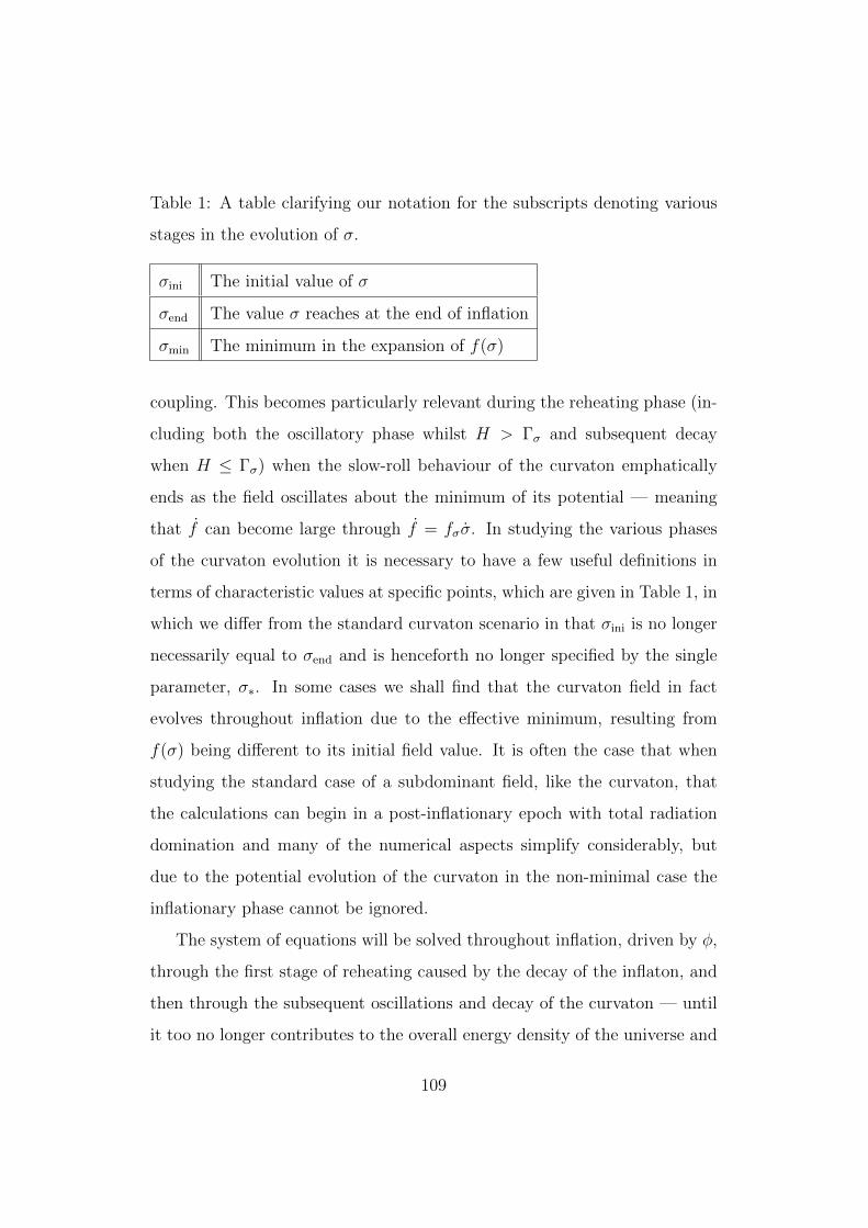
Table 1: A table clarifying our notation for the subscripts denoting various

stages in the evolution of σ.

σini The initial value of σ

σend The value σ reaches at the end of inflation

σmin The minimum in the expansion of f(σ)

coupling. This becomes particularly relevant during the reheating phase (in-

cluding both the oscillatory phase whilst H > Γσ and subsequent decay

when H ≤ Γσ) when the slow-roll behaviour of the curvaton emphatically

ends as the field oscillates about the minimum of its potential — meaning

that f can become large through f = fσσ. In studying the various phases

of the curvaton evolution it is necessary to have a few useful definitions in

terms of characteristic values at specific points, which are given in Table 1, in

which we differ from the standard curvaton scenario in that σini is no longer

necessarily equal to σend and is henceforth no longer specified by the single

parameter, σ∗. In some cases we shall find that the curvaton field in fact

evolves throughout inflation due to the effective minimum, resulting from

f(σ) being different to its initial field value. It is often the case that when

studying the standard case of a subdominant field, like the curvaton, that

the calculations can begin in a post-inflationary epoch with total radiation

domination and many of the numerical aspects simplify considerably, but

due to the potential evolution of the curvaton in the non-minimal case the

inflationary phase cannot be ignored.

The system of equations will be solved throughout inflation, driven by φ,

through the first stage of reheating caused by the decay of the inflaton, and

then through the subsequent oscillations and decay of the curvaton — until

it too no longer contributes to the overall energy density of the universe and

109

the curvature perturbation is finally frozen in. Studying the full evolution

like this requires a much greater range of scales, both physical and temporal,

to be tracked to sufficient accuracy that it results not only in complications

in writing the code, but also in very time consuming numerical integration

— the details of which will be looked at in Section 4.2. One key limitation

on the non-mimimal coupling should also be noted from the possibility that

σ can evolve during inflation, in that it requires the coupling to remain

sufficiently small so as not to allow the σ contribution to become significant

on inflationary scales — in which case the description of it as a curvaton or

even ‘curvaton-like’ field would be stretched and we’d very much be working

in a generic multi-field model.

To quantify this evolution of the curvaton during inflation, arising due to

the effective mass change caused by the explicit coupling to the Ricci scalar,

we can describe the evolution by considering Eq. (4.11) written instead in

terms of the e-fold number, N , and assuming slow-roll,

(3− ε)σ′ ≈ − VσH2

+ 3α(σ − σmin)(2− ε). (4.46)

If we then make the simplifying assumption that the mass of the curvaton is

small enough for the Vσ/H2 term (∝ m2

σ/m2φ) to be neglected, which is true

via the definition of the curvaton, this leaves

σ′ = 3α2− ε3− ε

(σ − σmin), (4.47)

which can be integrated to give

σ ∝ e3α 2−ε3−εN . (4.48)

Going further still, it is reasonable in many cases to assume that ε is small

throughout the relevant period of inflation and so in the limit that ε→ 0 we

110

are left with

σ ∝ e2αN , (4.49)

which is precisely what is observed in the numerics, a few examples of which

can be seen in Figure 18.

4.2 Numerics

Similarly to Section 3.4 we reformulate our second order differential equations

as first order equations written in terms of efold number, N , as follows,

y′0 = y1,

y′1 = (3− ε)y1 −VφH2− Γφy1

H,

y′2 = y3,

y′3 = (3− ε)y3 −VσH2

+fσR

2H2− Γσy3

H,

y′4 = −4y4 + ΓφHy21 + ΓσHy

23,

y′5 = 0, (4.50)

at background level (Equations (4.10) and (4.11))— where y5 was reserved

for possible matter decays to be included too and where the decays are only

‘switched on’ at the relevant times in the evolution. Here, we otherwise have

y0 = φ, y1 = φ′, y2 = σ, y3 = σ′ and y4 = ργ. Along with the background

equations we also require the perturbations — both of the fields and their

gravitational counterparts — and the now somewhat complicated expressions

for Ψ′′ coming from Eq. (4.8), δσ′′ and δf ′′ — which all depend on one

another. Continuing in terms of N , this can be achieved first by breaking

111

the expression for δf ′′ down into two parts in the following way,

δf ′′ = (fσδσ)′′ = fσσσσ′2δσ + 2fσσσ

′δσ′ + fσσσ′′δσ + fσδσ

′′

= δf ′′part1 + fσδσ′′, (4.51)

where δf ′′part1 denotes every other term within the expansion excluding the

one explicitly written. We can do the same then with the expansion of Ψ′′

to give

Ψ′′ = Ψ′′part1 +δf ′′

2f

= Ψ′′part2 +fσδσ

′′

2f, (4.52)

in which Ψ′′part2 has been updated to absorb the new terms from δf ′′part1 in the

last step too. Finally, we see in Eq. (4.19) that we can expand δR to reveal

the dependence on Ψ′′. Inputting the above expression for this into the δσ′′

equation finally gives us an equation we can evaluate numerically, which no

longer revolves around so many interdependencies. Such that we now have

δσ′′ = δσ′′part1 − 3Ψ′′fσ

= δσ′′part2 − 3Ψ′′part2fσ −3f 2

σδσ′′

2f, (4.53)

which can be rearranged to give

δσ′′ =δσ′′part2 − 3Ψ′′part2fσ

1 + 3f2σ

2f

, (4.54)

in which the terms contained within δσ′′part2 and Ψ′′part2 can be readily found

from their respective full expressions, after tracing the previous work back.

So for the perturbation equations we are left with the following, all repeated

112

four times as described in the earlier numerics section,

y′6 = y7

y′7 = (ε− 4)y7 +δf ′

f− δff ′

f 2+ (2ε− 3)

(y6 −

δf

f

)+

1

2f

[y1y9 + y3y11

− (y21 + y2

3)

(y6 −

δf

f

)− Vφy8

H2− Vσy10

H2− 2

(y6 −

δf

f

)(f ′′ − εf)′

− f ′(y7 + 2y6 − 2

δf

f

)− δf

f

(y4

3H2+y2

1 + y23

2− V

H2− εf ′ − f ′′ + 2f ′

)− (ε− 2)δf ′ + fσσσy

23y10 + fσσy3y11 + fσσy10

((ε− 3)y3 −

VσH2

+fσ

2H2− Γσy3

H

)+ fσσy3y11 +

k2

a2

δf

H2+

y12

3H2

]+fσδσ

′′

2f

y′8 = y9

y′9 =

(ε− 3− Γφ

H

)y9 −

(k2

a2+ Vφφ

)y8

H2+

(4y7 −

δf

f+δff ′

f 2

)y1

− 2

H2

(y6 −

δf

f

)(Vφ +HΓφ)− Vφσ

y′10 = y11

y′11 =1

1 + 3f2σ

2f

[(ε− 3− Γφ

H

)y11 −

(k2

a2− fσσR

2+ Vσσ

)y10

H2

+

(4y7 −

δf

f+δff ′

f 2

)y3 −

2

H2

(y6 −

δf

f

)(Vσ +HΓσ)− Vφσy8

H2

−(

12y7 −k2

a2H2

(y6 +

δf

f

)+ 3

(y7 −

δf ′

f+δff ′

f 2

)− 3εy7 + 3Ψ′′part2

)fσ

]

y′12 = −4y12 + 4y4

(y7 −

δf ′

f+δff ′

f 2

)− 2

k2

a2

(y7 + y6 −

δf

f

)

+ 2HΓφ

y1y9 +y2

1

(y6 − δf

f

)2

+ 2HΓσ

y3y11 +y2

3

(y6 − δf

f

)2

y′13 = 0 (4.55)

113

where the subscripts 7 and 8 relate to the Ψ′′ equation, 8–11 to δφ′′ and δσ′′

respectively and 12 and 13 to the energy densities of radiation and matter

(the latter of which we ignore and therefore set to zero).

We set the initial conditions for each mode, k, such that k∗ = 50ainiHini

by first running through the background up to the end of inflation (when

ε = 1), using this to ascertain the appropriate field value for the inflaton,

φini. The initial conditions of the perturbations are then set to the Bunch-

Davies vacuum (for one field, whilst the other field takes an initial value of

zero — see Section 3.4 for details — and vice versa) at this point and the

full code is run. The time parameter, N , is set to be equal to zero at horizon

exit and our results are plotted against this. When working in these units

the scale of aini becomes arbitrary as results can be scaled afterwards. We

choose aini = 1.0

The code is split into four sections, each solved successively with the end

values to each one used as the initial conditions in the next, with tolerance

parameters altered accordingly as the scales decrease throughout the sections:

1. Inflation: This covers the period from N = 0 through to when the

inflaton crosses the minimum of the potential and begins to oscillate,

at which point we move on to the next stage by switching on the de-

cay. This causes no inconsistencies as the decay rate is typically much

smaller than the dominant friction term, 3Hφ, at this point.

2. Inflaton decay: Covering the period through the first part of reheat-

ing, but before the secondary field has begun to decay, we now set

Γφ 6= 0. This continues until the curvaton, σ, has also dropped from its

value at the end of inflation (which occurs when H ≈ mσ) and oscillates

about its minimum.

114

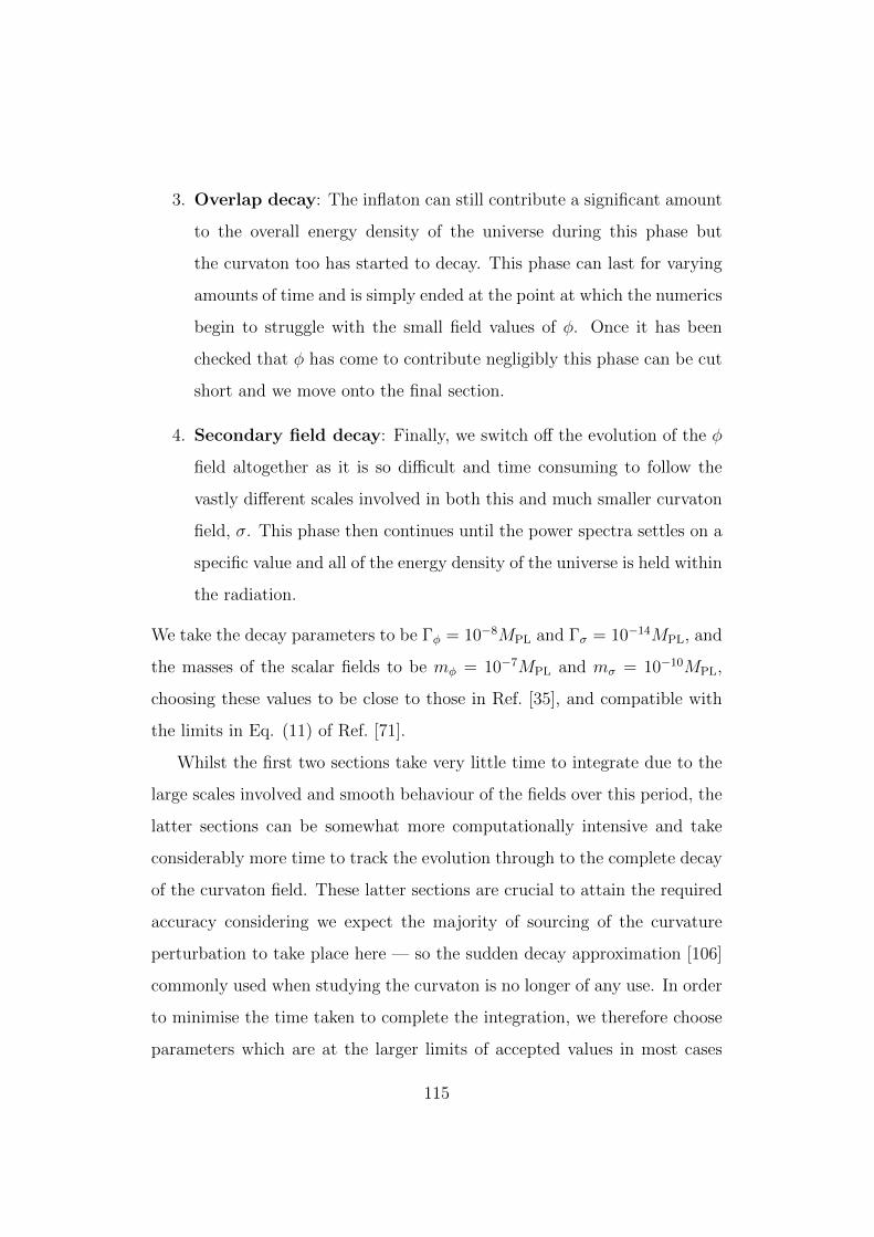
3. Overlap decay: The inflaton can still contribute a significant amount

to the overall energy density of the universe during this phase but

the curvaton too has started to decay. This phase can last for varying

amounts of time and is simply ended at the point at which the numerics

begin to struggle with the small field values of φ. Once it has been

checked that φ has come to contribute negligibly this phase can be cut

short and we move onto the final section.

4. Secondary field decay: Finally, we switch off the evolution of the φ

field altogether as it is so difficult and time consuming to follow the

vastly different scales involved in both this and much smaller curvaton

field, σ. This phase then continues until the power spectra settles on a

specific value and all of the energy density of the universe is held within

the radiation.

We take the decay parameters to be Γφ = 10−8MPL and Γσ = 10−14MPL, and

the masses of the scalar fields to be mφ = 10−7MPL and mσ = 10−10MPL,

choosing these values to be close to those in Ref. [35], and compatible with

the limits in Eq. (11) of Ref. [71].

Whilst the first two sections take very little time to integrate due to the

large scales involved and smooth behaviour of the fields over this period, the

latter sections can be somewhat more computationally intensive and take

considerably more time to track the evolution through to the complete decay

of the curvaton field. These latter sections are crucial to attain the required

accuracy considering we expect the majority of sourcing of the curvature

perturbation to take place here — so the sudden decay approximation [106]

commonly used when studying the curvaton is no longer of any use. In order

to minimise the time taken to complete the integration, we therefore choose

parameters which are at the larger limits of accepted values in most cases

115

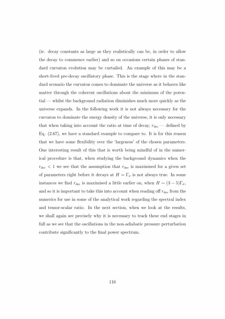
(ie. decay constants as large as they realistically can be, in order to allow

the decay to commence earlier) and so on occasions certain phases of stan-

dard curvaton evolution may be curtailed. An example of this may be a

short-lived pre-decay oscillatory phase. This is the stage where in the stan-

dard scenario the curvaton comes to dominate the universe as it behaves like

matter through the coherent oscillations about the minimum of the poten-

tial — whilst the background radiation diminishes much more quickly as the

universe expands. In the following work it is not always necessary for the

curvaton to dominate the energy density of the universe, it is only necessary

that when taking into account the ratio at time of decay, rdec — defined by

Eq. (2.67), we have a standard example to compare to. It is for this reason

that we have some flexibility over the ‘largeness’ of the chosen parameters.

One interesting result of this that is worth being mindful of in the numer-

ical procedure is that, when studying the background dynamics when the

rdec < 1 we see that the assumption that rdec is maximised for a given set

of parameters right before it decays at H = Γσ is not always true. In some

instances we find rdec is maximised a little earlier on, when H ∼ (3 − 5)Γσ,

and so it is important to take this into account when reading off rdec from the

numerics for use in some of the analytical work regarding the spectral index

and tensor-scalar ratio. In the next section, when we look at the results,

we shall again see precisely why it is necessary to track these end stages in

full as we see that the oscillations in the non-adiabatic pressure perturbation

contribute significantly to the final power spectrum.

116

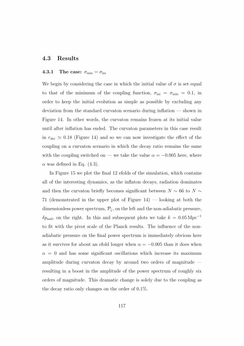
4.3 Results

4.3.1 The case: σmin = σini

We begin by considering the case in which the initial value of σ is set equal

to that of the minimum of the coupling function, σini = σmin = 0.1, in

order to keep the initial evolution as simple as possible by excluding any

deviation from the standard curvaton scenario during inflation — shown in

Figure 14. In other words, the curvaton remains frozen at its initial value

until after inflation has ended. The curvaton parameters in this case result

in rdec ' 0.18 (Figure 14) and so we can now investigate the effect of the

coupling on a curvaton scenario in which the decay ratio remains the same

with the coupling switched on — we take the value α = −0.005 here, where

α was defined in Eq. (4.3).

In Figure 15 we plot the final 12 efolds of the simulation, which contains

all of the interesting dynamics, as the inflaton decays, radiation dominates

and then the curvaton briefly becomes significant between N ∼ 66 to N ∼

71 (demonstrated in the upper plot of Figure 14) — looking at both the

dimensionless power spectrum, Pζ , on the left and the non-adiabatic pressure,

δpnad, on the right. In this and subsequent plots we take k = 0.05 Mpc−1

to fit with the pivot scale of the Planck results. The influence of the non-

adiabatic pressure on the final power spectrum is immediately obvious here

as it survives for about an efold longer when α = −0.005 than it does when

α = 0 and has some significant oscillations which increase its maximum

amplitude during curvaton decay by around two orders of magnitude —

resulting in a boost in the amplitude of the power spectrum of roughly six

orders of magnitude. This dramatic change is solely due to the coupling as

the decay ratio only changes on the order of 0.1%.

117

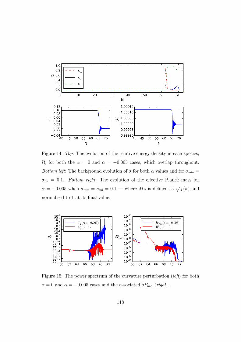
Figure 14: Top: The evolution of the relative energy density in each species,

Ωi for both the α = 0 and α = −0.005 cases, which overlap throughout.

Bottom left: The background evolution of σ for both α values and for σmin =

σini = 0.1. Bottom right: The evolution of the effective Planck mass for

α = −0.005 when σmin = σini = 0.1 — where MP is defined as√f(σ) and

normalised to 1 at its final value.

Figure 15: The power spectrum of the curvature perturbation (left) for both

α = 0 and α = −0.005 cases and the associated δPnad (right).

118

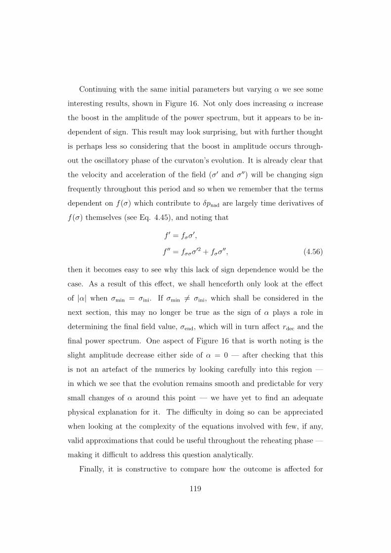
Continuing with the same initial parameters but varying α we see some

interesting results, shown in Figure 16. Not only does increasing α increase

the boost in the amplitude of the power spectrum, but it appears to be in-

dependent of sign. This result may look surprising, but with further thought

is perhaps less so considering that the boost in amplitude occurs through-

out the oscillatory phase of the curvaton’s evolution. It is already clear that

the velocity and acceleration of the field (σ′ and σ′′) will be changing sign

frequently throughout this period and so when we remember that the terms

dependent on f(σ) which contribute to δpnad are largely time derivatives of

f(σ) themselves (see Eq. 4.45), and noting that

f ′ = fσσ′,

f ′′ = fσσσ′2 + fσσ

′′, (4.56)

then it becomes easy to see why this lack of sign dependence would be the

case. As a result of this effect, we shall henceforth only look at the effect

of |α| when σmin = σini. If σmin 6= σini, which shall be considered in the

next section, this may no longer be true as the sign of α plays a role in

determining the final field value, σend, which will in turn affect rdec and the

final power spectrum. One aspect of Figure 16 that is worth noting is the

slight amplitude decrease either side of α = 0 — after checking that this

is not an artefact of the numerics by looking carefully into this region —

in which we see that the evolution remains smooth and predictable for very

small changes of α around this point — we have yet to find an adequate

physical explanation for it. The difficulty in doing so can be appreciated

when looking at the complexity of the equations involved with few, if any,

valid approximations that could be useful throughout the reheating phase —

making it difficult to address this question analytically.

Finally, it is constructive to compare how the outcome is affected for

119

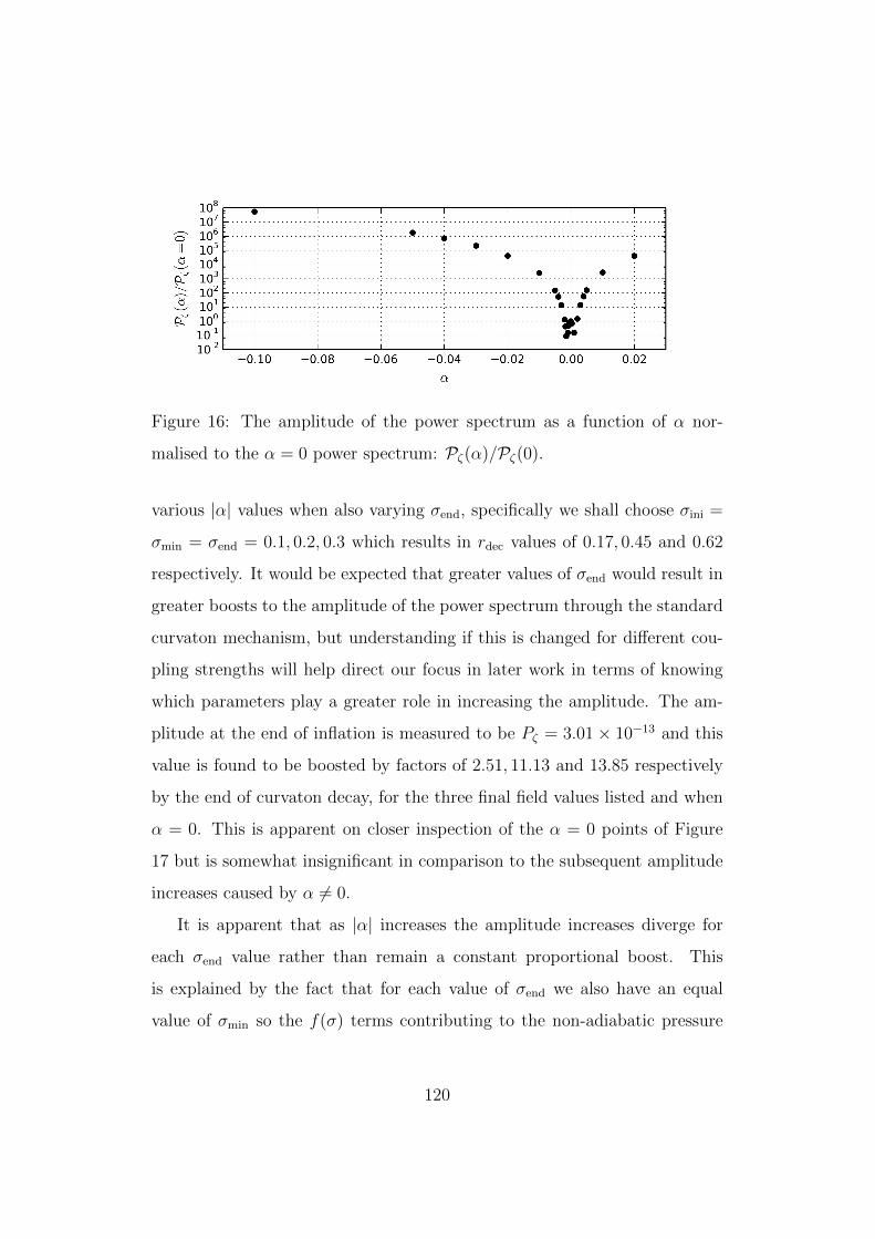
Figure 16: The amplitude of the power spectrum as a function of α nor-

malised to the α = 0 power spectrum: Pζ(α)/Pζ(0).

various |α| values when also varying σend, specifically we shall choose σini =

σmin = σend = 0.1, 0.2, 0.3 which results in rdec values of 0.17, 0.45 and 0.62

respectively. It would be expected that greater values of σend would result in

greater boosts to the amplitude of the power spectrum through the standard

curvaton mechanism, but understanding if this is changed for different cou-

pling strengths will help direct our focus in later work in terms of knowing

which parameters play a greater role in increasing the amplitude. The am-

plitude at the end of inflation is measured to be Pζ = 3.01× 10−13 and this

value is found to be boosted by factors of 2.51, 11.13 and 13.85 respectively

by the end of curvaton decay, for the three final field values listed and when

α = 0. This is apparent on closer inspection of the α = 0 points of Figure

17 but is somewhat insignificant in comparison to the subsequent amplitude

increases caused by α 6= 0.

It is apparent that as |α| increases the amplitude increases diverge for

each σend value rather than remain a constant proportional boost. This

is explained by the fact that for each value of σend we also have an equal

value of σmin so the f(σ) terms contributing to the non-adiabatic pressure

120

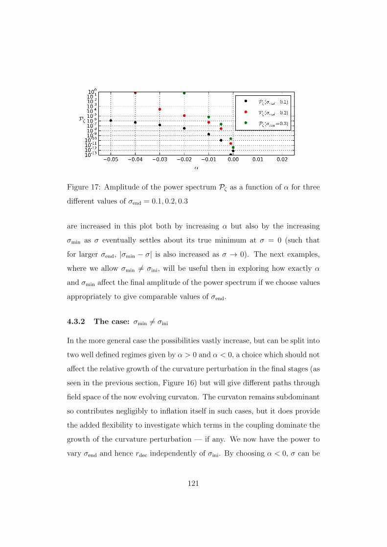
Figure 17: Amplitude of the power spectrum Pζ as a function of α for three

different values of σend = 0.1, 0.2, 0.3

are increased in this plot both by increasing α but also by the increasing

σmin as σ eventually settles about its true minimum at σ = 0 (such that

for larger σend, |σmin − σ| is also increased as σ → 0). The next examples,

where we allow σmin 6= σini, will be useful then in exploring how exactly α

and σmin affect the final amplitude of the power spectrum if we choose values

appropriately to give comparable values of σend.

4.3.2 The case: σmin 6= σini

In the more general case the possibilities vastly increase, but can be split into

two well defined regimes given by α > 0 and α < 0, a choice which should not

affect the relative growth of the curvature perturbation in the final stages (as

seen in the previous section, Figure 16) but will give different paths through

field space of the now evolving curvaton. The curvaton remains subdominant

so contributes negligibly to inflation itself in such cases, but it does provide

the added flexibility to investigate which terms in the coupling dominate the

growth of the curvature perturbation — if any. We now have the power to

vary σend and hence rdec independently of σini. By choosing α < 0, σ can be

121

pulled towards its local minimum prior to decay whilst α > 0 has the opposite

effect — pushing it away. This second case soon becomes problematic for

values of α ≥ 0.05 due to the exponential increase in the field value shown in

Eq. (4.49) — leading to possible curvaton domination during inflation and,

beyond that, problems in the numerics in as σ →∞. Due to the symmetry

in α this need not be too concerning as we can investigate the effects of α

itself still using negative values alone, the primary benefit of positive α values

comes in being able to alter the trajectory of σ in a few controllable cases to

demonstrate that the results continue to be independent of sign, which can

be done by choosing varying values for σini and then matching them up with

α values that give comparable values of σend to the negative case.

In the final paragraph of the previous section, it was hinted at that the

value of σmin seems to dominate the boost in the curvature perturbation

over the value of σend and we can now confirm this — being most simply

demonstrated in Figure 18. This plot shows results from two cases, both with

σmin = 0.1 but now with differering initial values, given by σini = 0.1 and 0.3

respectively. α is allowed to run over the values used in the σini = σmin case

looked at previously which now gives various values of σend in the σini = 0.3

case as 0 > α > −0.03 results in 0.3 > σend > 0.1, while α < −0.03 gives

σend = 0.1 (as can be seen in the right hand side of Figure 18), whilst for the

σini = 0.1 case there remains no evolution. The left hand side of Figure 18

shows that for larger values of α the final amplitudes of the power spectra

converge but for smaller values there remains a significant difference. This

can be explained by the role that σend plays in that these values of α have not

been given enough time for the fields to evolve to the same final σ value —

but it can be seen that the difference between each amplitude is subdominant

in comparison to the much larger increases visible as α increases. This will

122

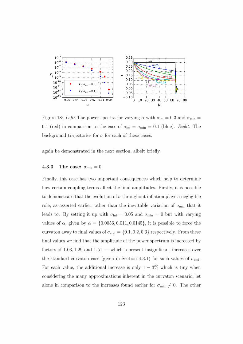
Figure 18: Left: The power spectra for varying α with σini = 0.3 and σmin =

0.1 (red) in comparison to the case of σini = σmin = 0.1 (blue). Right: The

background trajectories for σ for each of these cases.

again be demonstrated in the next section, albeit briefly.

4.3.3 The case: σmin = 0

Finally, this case has two important consequences which help to determine

how certain coupling terms affect the final amplitudes. Firstly, it is possible

to demonstrate that the evolution of σ throughout inflation plays a negligible

role, as asserted earlier, other than the inevitable variation of σend that it

leads to. By setting it up with σini = 0.05 and σmin = 0 but with varying

values of α, given by α = 0.0056, 0.011, 0.0145, it is possible to force the

curvaton away to final values of σend = 0.1, 0.2, 0.3 respectively. From these

final values we find that the amplitude of the power spectrum is increased by

factors of 1.03, 1.29 and 1.51 — which represent insignificant increases over

the standard curvaton case (given in Section 4.3.1) for such values of σend.

For each value, the additional increase is only 1 − 3% which is tiny when

considering the many approximations inherent in the curvaton scenario, let

alone in comparison to the increases found earlier for σmin 6= 0. The other

123

important aspect of this test is that it demonstrates categorically that σmin

plays the dominant role in the growth of the amplitude of the power spectrum,

as we continue to vary both α and σend and yet still get essentially standard

curvaton results since |σ − σmin| is now small during the oscillatory phase.

4.4 Some concluding remarks

In this Chapter, the stabilisation of the Planck mass has been considered

via a secondary field that is non-minimally coupled to gravity and plays a

negligible role during inflation itself. The work has been done in the Jordan

frame in order to treat the decays and reheating in the standard way and

the evolution of the scale invariant power spectrum has been tracked via the

non-adiabatic pressure perturbation — which is also frame independent. The

work was primarily numerical due to the complexity of the equations and the

lack of reasonable approximations in such a case, but this has not retarded

investigations into how exactly the primordial power spectrum is affected by

the late-stabilisation of the Planck mass.

It had previously been shown that such a coupling could induce changes in

the final power spectrum via additional terms in the non-adiabatic pressure

perturbation feeding into the curvature perturbation on super-horizon scales

[86] but the effect had yet to be quantified. Here it has been shown that

the terms proportional to f, f and f can play a significant role in increasing

the amplitude as the coupled curvaton-like field oscillates and decays — with

the quickly varying motion of the field feeding in through the then relatively

large f and f terms in particular. The actual increase in the amplitude is

much larger than might have been expected for relatively small changes in

the Planck mass, varying by many orders of magnitude for variations of the

Planck mass of roughly 0.01− 1%.

124

Due to the insignificance of the secondary field throughout inflation, the

relatively small amount of evolution imparted in some cases by the coupling

and the tiny variation in Planck mass, the spectral index linked to the curva-

ton field alone remains unchanged from the standard case (which equates to

a value of ns ' 0.98) and so we can proceed to investigate how the observed

spectral index is then found from the non-minimally coupled case. Using the

same parameterisation as in the standard curvaton case, the effect of this am-

plitude boost can then be linked to the spectral index, ns and tensor-scalar

ratio, rTS by Eq. (2.80) and [107], which is

Pζ = P(φ)ζ + P(σ)

ζ = (1 +R)P(φ)ζ , (4.57)

where

R =P(σ)ζ

P(φ)ζ

. (4.58)

This gives

ns − 1 = −2ε+ 2ησ −4ε− 2ηφ

1 +Rand rTS =

16ε

1 +R, (4.59)

using the usual definitions of the slow roll parameters, evaluated at horizon

crossing. It is clear that these two important observational quantities depend

only on the final ratio, R, and not the mechanism by which the curvature

perturbation is sourced — placing constraints on the values some of our

parameters can take according to the latest Planck data [73]. It is relatively

easy to see, taking Figure 15 as an example, that even for values of α =

−0.005 and σmin = 0.1 we find R ∼ 107 (by comparing the final amplitude of

the power spectrum to that seen prior to curvaton decay, at N ∼ 65) in which

case we are very much in the regime of the pure-curvaton limit in terms of

ns and rTS — which is already at odds with observational data. As such, it

125

remains to be seen whether fundamental theories of particle physics will give

rise to such a simple model similar to this which can be readily constrained

from the work above.

126

5 Conclusions and a future direction

There are currently an abundance of models of inflation available to cosmolo-

gists that still remain viable in the face of increasingly precise measurements

of the the cosmos — both from the first moments after the beginning of

time and in the current accelerating epoch. Some such descriptions of the

universe are motivated phenomenologically, some experimentally and others

purely from theoretical considerations such as those that result from higher

energy theories such as string theory, many of which have distinctive pre-

dictions in their observational signatures. It is important to understand the

features and problems with each class of model and to accurately predict

their observational signatures in order to eventually rule them out as real

data comes in and knowledge about our universe on the largest of scales in-

creases — with the aim of finally narrowing the vast array of options down

to (perhaps optimistically) a single viable theory of the cosmos.

In this thesis a wide range of such models have been considered, rang-

ing from the theoretical non-canonical couplings and scalar-tensor theories

considered in Chapters 3 and 4 to the phenomenological descriptions of re-

heating used in Chapter 4 and, soon, in this chapter too. These models

have been studied both analytically and numerically in attempts to find a

balance between understanding the physical interpretations of the various

results found whilst maintaining an accuracy only available via numerical

simulations. In Chapter 3, an approximation of the power spectra was found

for both canonical and non-canonical models of inflation and compared to

the numerics to ascertain the accuracy of such simplifications. The approxi-

mation went to second order in the slow-roll parameters, extending the work

done previously to the non-canonical case with the aim of gaining greater

127

insight into the importance of such newly defined non-canonical equivalents

to the slow-roll parameters, namely ξ21 and ξ2. We studied both the curvature

power spectrum, the isocurvature power spectrum and kept a close eye on

the interaction between the two that leads to the growth of the curvature

perturbation. In this work we found an improved analytical approximation,

even in the canonical-case when it came to certain potentials, over previous

work [66] and a vast improvement over the accuracy of the first order ap-

proximations used in non-canonical studies prior to this work. Not only this,

but our approximation also takes into account the possibility of higher order

coupling terms — allowing greater accuracy when considering couplings of

the form eβφn

where n > 1. The great advantage of such improved analytical

approximations is the understanding of which aspects of a model dominate

in their contributions to the final curvature power spectra, and we have been

able to clearly study this by simply removing various terms in the expressions

to see how greatly they affect the final results.

In Chapter 4, we studied how a curvaton-like field would be affected by

non-minimally coupling it to gravity — effectively allowing the gravitational

constant to vary until after inflation has ended. The work was done entirely in

the Jordan frame so as to ensure that the description of various decays could

be kept as simple as possible and we found some surprising results. Whilst

the spectral index and tensor-scalar ratio remain consistent with those of a

standard curvaton scenario we find a significant change in the amplitude of

the power spectrum for such non-minimally coupled models, owing to the

presence of terms proportional to the time dependence of the coupling, f(σ),

in the non-adiabatic pressure perturbation. It has long been known that the

non-adiabatic pressure perturbation can source the curvature perturbation

(in a frame independent manner) but the inclusion of these additional terms

128

( ˙f(σ), ¨f(σ)), particularly during the oscillatory motion of the curvaton re-

heating phase, vastly increased the magnitude of the sourcing to the extent

that a variation of the Planck mass of less than 1% can lead to an increase

in the magnitude of the curvature power spectrum of over 103. We have

also shown that the primary cause of this is not due to the evolution of the

curvaton (and hence, Planck mass) during inflation — which has next to no

effect due to the dominance of the inflaton’s behaviour at this time — but

rather it comes from the values of α and σmin in the coupling itself.

So far, we have considered some of the simpler multi-field models, models

of inflation with a non-canonical coupling — linking the fields themselves

together, and finally, models of inflation with one of the fields coupled to

gravity. It has been repeatedly demonstrated that such couplings and mod-

ifications to standard inflationary scenarios regularly throw up new and in-

teresting possibilities along with important changes to the observational sig-

natures of interest today, none more so than example of the late stabilisation

of the Planck mass in Chapter 4 which also demonstrates the importance of

understanding the post inflationary behaviour of the universe as the main

effects of the coupling only come to light during reheating. But why stop

there? There are two natural extensions to this work:

1. Look more carefully at the reheating phase and how it might be affected

by taking preheating into account. When considering the form of δpnad

in Chapter 4 it is difficult to see the amplitude increase being changed

in qualitative terms — as it seems well explained as to where it would

come from in the reheating phase (relating to f , f etc.) — but that is

not to say that quantitative changes could not be found. It could well

be interesting to even investigate how preheating affects the decay of

the inflaton, never mind the curvaton decay, and subsequent curvaton

129

decay ratios.

2. Further extend the gravitational coupling by including higher order

gravitational terms — such as the Gauss-Bonnet term.

We will focus on the second of these points, for now, before then showing

how the first point becomes even more important in such scenarios as the

dynamics of inflation and the subsequent reheating are dramatically altered.

5.1 A Gauss-Bonnet encore

So what is Gauss-Bonnet inflation and why is it useful? There has been some

interest in Gauss-Bonnet terms which are derived from superstring theory as

one of the simplest correction terms to the lowest order effective action [164]

as they can help in efforts to explain the late time acceleration of the universe

and also manage avoid the initial Big Bang singularity [165]. This term is

defined by,

R2GB = RµνρσR

µνρσ − 4RµνRµν +R2, (5.1)

and enters the action (shown here with a single field, but easily extended to

multiple fields) via the additional term in

S =

∫d4x√−g[R

2− 1

2gµν∂µφ∂νφ− V (φ)− 1

2ξ(φ)R2

GB + Lint

], (5.2)

where the coupling to the field, φ is given by ξ(φ).

A significant amount of interest has come about due to the fact that a

Gauss-Bonnet term included with some very general inflationary potentials

can lead to non-oscillatory (NO) behaviour in what would normally be the

reheating phase at the end of inflation — which may give rise to simple models

of quintessential inflation in which the late time acceleration of the universe

130

is explained by the same field that causes the inflationary expansion in the

first place [166, 167]. In order to investigate such models further it is first

necessary to understand a few things about inflation itself (and the governing

equations of motion) along with the transition out of an inflationary epoch in

such scenarios — both in the case of standard models where normal reheating

can still occur and in NO models.

5.1.1 The equations of motion

With the inclusion of the Gauss-Bonnet term, the field equations take the

following form [168],

φ+ 3Hφ+ Vφ + 12ξφH2(H +H2) = 0, (5.3)

along with the Friedmann equations,

3H2 =φ2

2+ V (φ) + 12ξH3 and (5.4)

H = − φ2

2+ 2H2ξ + 2Hξ

(2H −H2

). (5.5)

It is here that we come across the first problem in numerically evaluating

these equations — the standard method of calculating the Hubble parameter

from the background Klein-Gordon equation no longer works due to addi-

tional term including H on the right hand side of Eq. (5.4). As such, it

becomes necessary to integrate Eq. (5.5) alongside the Klein-Gordon equa-

tion which makes the numerics potentially somewhat more involved and oc-

casionally problematic, as we shall come to later. In the subsequent sections,

we will follow convention and introduce a new coupling parameter, α, which

is defined in terms of the potential and coupling term together. Given some

functions, for example a simple power law potential and inverse power law

131

coupling,

V (φ) = V0φp and ξ(φ) = ξ0φ

−q, (5.6)

we can define α as,

α =4V0ξ0

3. (5.7)

5.1.2 Reheating in Gauss-Bonnet inflation

It has already been mentioned that in some cases, possibly being what makes

these models attractive, the inflaton fails to oscillate at the end of inflation

and as such reheating cannot occur in the usual way. Whether or not this

is the case, interesting questions arise regarding the nature of reheating and

precisely how it might be affected. Should the inflaton oscillate, would we

find modifications to the reheating temperature both in terms of perturbative

reheating and preheating and would the power spectra be affected in a similar

way to the late stabilisation of the gravitational constant in the previous

Chapter? Does the inflaton decay completely or can some remnant remain

and still be responsible for the dark energy observed today — without causing

problems with the intermediate expansion history of the universe?

In NO models, many of the same questions remain about the intermediate

expansion history but a new method entirely is required to reheat the universe

in the first place — and this can be done in a number of ways, which shall

be summarised here. The first option is gravitational reheating described by

[169, 170, 171] in which massless particles are created due to the expansion

of space-time [172]. The major drawback of this reheating mechanism is that

it is relatively inefficient in comparison to the mechanisms discussed next.

Despite the particle production being so inefficient, it can still work as at this

stage in the evolution of the universe the inflaton energy density is dominated

132

by the kinetic contribution rather than the potential contribution that had

driven inflation to this point (ρφ ∼ φ/2) and as such, scales proportional to

a−6 in comparison to the radiation which scales as a−4. So despite being sub-

dominant initially it does not take long for the universe to become dominated

by the decay products. Another option is instant preheating [173] — which

also no longer requires a minimum of the potential to be effective and is

much more efficient than gravitational reheating [174]. If it is assumed that

the inflaton interacts with another scalar field, χ, via the interaction term

given in Eq. (1.51) it can be shown that in many situations preheating can

be completed not after numerous oscillations, but in the first instant of the

term becoming important. Much like if a regular, oscillatory scenario was

cut off at the moment the first decay products appear. The key to this

effect is to allow the χ particles to decay quickly into fermions — but not

before their energy density has grown by up to 2 orders of magnitude in

comparison to a standard preheating scenario due to the continued rolling of

the inflaton field [175]. This is an attractive mechanism due to the efficiency

and simplicity of the idea, but may require a certain amount of fine tuning

in order to result in realistic models of the universe. The final option, and

the one most thoroughly considered here, is to return to the curvaton. This

allows us to study the effects of introducing radiation (and matter) in NO

models without the need to further couple the Gauss-Bonnet inflaton field

— with predictable effects due to the widely studied nature of the curvaton

itself both by other authors and earlier in this thesis.

5.1.3 Observational constraints

To begin this short section, we take the following expressions from [176] in

order to later calculate the spectral index and tensor-scalar ratio in slow-roll

133

Gauss-Bonnet inflation,

ns = −2ε1 −2ε1ε2 − δ1δ2

2ε1 − δ1

,

rTS = 8(2ε1 − δ1), (5.8)

where,

ε1 =Q

2

VφV,

ε2 = −Q(VφφVφ− VφV

+Qφ

Q

),

δ1 = −4Q

3ξφV,

δ2 = −Q(ξφφξφ

+VφV

+Qφ

Q

), (5.9)

and

Q ≡ VφV

+4V ξφ

3. (5.10)

These will be useful in quickly determining if the inflationary model itself

is favoured or not in comparison to current data, prior to considering whether

the behaviour through reheating constrains the model. The two other (closely

linked) aspects of each model that shall be focused on here is whether or not a

potential and coupling allow for the inflaton to become sub-dominant during

a radiation dominated epoch — choosing to loosely define this as Ωφ < 0.2

at the upper end of realistic constraints [177] — and then whether or not it

can eventually regain its dominance and help explain dark energy. It should

be noted that the precise constraints on Ωφ are still up for debate, see [178]

and [179] for opposing ends of the spectrum.

5.1.4 A few example models

We shall continue to follow [176] in their choice of models, with a couple of

variations, and give some results that demonstrate the main properties we

134

have found. We begin with a potential and coupling defined by

V (φ) = V0φp and ξ(φ) = ξ0φ

−q, (5.11)

where we initially take p = q = 2 but the results are equally applicable to

p = q = 4. In such a situation, even taking a relatively massive curvaton

(mσ = mφ/100) with an unreasonably large decay rate (Γσ = mσ/10) we find

that it is difficult, if not impossible, to find a situation in which the curvaton

or radiation dominates for any period of time. With α = 0, returning to the

standard case, this results in a curvaton decay ratio of ∼ 0.45 (although it

should be noted that it is hard to compare this to when α 6= 0 due to the

usual oscillations occurring) whereas with α = 10−4, 10−3 or 10−2 we find

this ratio consistently reducing, with the produced radiation even more sub-

dominant. An example case, indicative of results for every combination thus

far attempted, using α = 10−2, is given in Figure 19 where we see that Ωγ

maximally and only temporarily reaches 0.01. When looking at the energy

densities themselves, we see that the coupled inflaton field continues to lose

energy until it approaches equality with the curvaton field before leveling

off and continuing to dominate — not what would be expected if this was

behaving as a kinetic-dominated field, losing energy faster than radiation.

Considering, now, an exponential coupling of the form,

ξ(φ) = ξ0e−qφ, (5.12)

along with the same quadratic potential as before and using some parameter

choices that fit well with observations of the spectral index and tensor-scalar

ratio — namely, α = 0.03 and q = 0.2 . We find that for this potential the

field oscillates as normal and completely decays away, although it is difficult

to numerically track the field for long after radiation domination occurs due

to the steep drop off in its energy density causing quite a discrepancy between

135

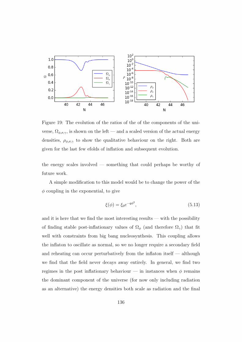
Figure 19: The evolution of the ratios of the of the components of the uni-

verse, Ωφ,σ,γ, is shown on the left — and a scaled version of the actual energy

densities, ρφ,σ,γ to show the qualitative behaviour on the right. Both are

given for the last few efolds of inflation and subsequent evolution.

the energy scales involved — something that could perhaps be worthy of

future work.

A simple modification to this model would be to change the power of the

φ coupling in the exponential, to give

ξ(φ) = ξ0e−qφ2

, (5.13)

and it is here that we find the most interesting results — with the possibility

of finding stable post-inflationary values of Ωφ (and therefore Ωγ) that fit

well with constraints from big bang nucleosynthesis. This coupling allows

the inflaton to oscillate as normal, so we no longer require a secondary field

and reheating can occur perturbatively from the inflaton itself — although

we find that the field never decays away entirely. In general, we find two

regimes in the post inflationary behaviour — in instances when φ remains

the dominant component of the universe (for now only including radiation

as an alternative) the energy densities both scale as radiation and the final

136

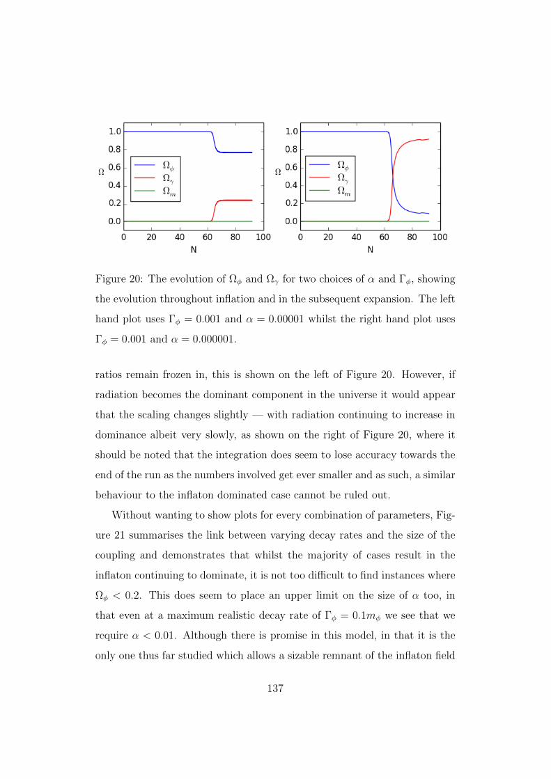
Figure 20: The evolution of Ωφ and Ωγ for two choices of α and Γφ, showing

the evolution throughout inflation and in the subsequent expansion. The left

hand plot uses Γφ = 0.001 and α = 0.00001 whilst the right hand plot uses

Γφ = 0.001 and α = 0.000001.

ratios remain frozen in, this is shown on the left of Figure 20. However, if

radiation becomes the dominant component in the universe it would appear

that the scaling changes slightly — with radiation continuing to increase in

dominance albeit very slowly, as shown on the right of Figure 20, where it

should be noted that the integration does seem to lose accuracy towards the

end of the run as the numbers involved get ever smaller and as such, a similar

behaviour to the inflaton dominated case cannot be ruled out.

Without wanting to show plots for every combination of parameters, Fig-

ure 21 summarises the link between varying decay rates and the size of the

coupling and demonstrates that whilst the majority of cases result in the

inflaton continuing to dominate, it is not too difficult to find instances where

Ωφ < 0.2. This does seem to place an upper limit on the size of α too, in

that even at a maximum realistic decay rate of Γφ = 0.1mφ we see that we

require α < 0.01. Although there is promise in this model, in that it is the

only one thus far studied which allows a sizable remnant of the inflaton field

137

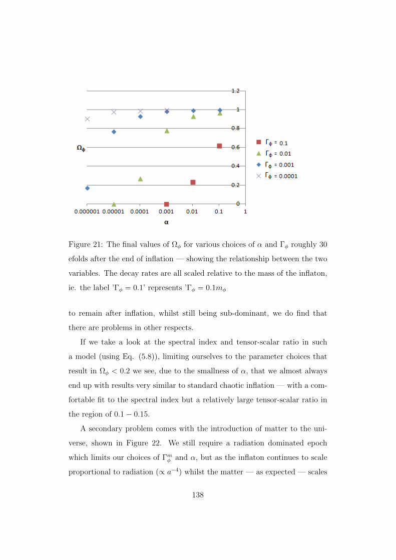
Figure 21: The final values of Ωφ for various choices of α and Γφ roughly 30

efolds after the end of inflation — showing the relationship between the two

variables. The decay rates are all scaled relative to the mass of the inflaton,

ie. the label ’Γφ = 0.1’ represents ’Γφ = 0.1mφ

to remain after inflation, whilst still being sub-dominant, we do find that

there are problems in other respects.

If we take a look at the spectral index and tensor-scalar ratio in such

a model (using Eq. (5.8)), limiting ourselves to the parameter choices that

result in Ωφ < 0.2 we see, due to the smallness of α, that we almost always

end up with results very similar to standard chaotic inflation — with a com-

fortable fit to the spectral index but a relatively large tensor-scalar ratio in

the region of 0.1− 0.15.

A secondary problem comes with the introduction of matter to the uni-

verse, shown in Figure 22. We still require a radiation dominated epoch

which limits our choices of Γmφ and α, but as the inflaton continues to scale

proportional to radiation (∝ a−4) whilst the matter — as expected — scales

138

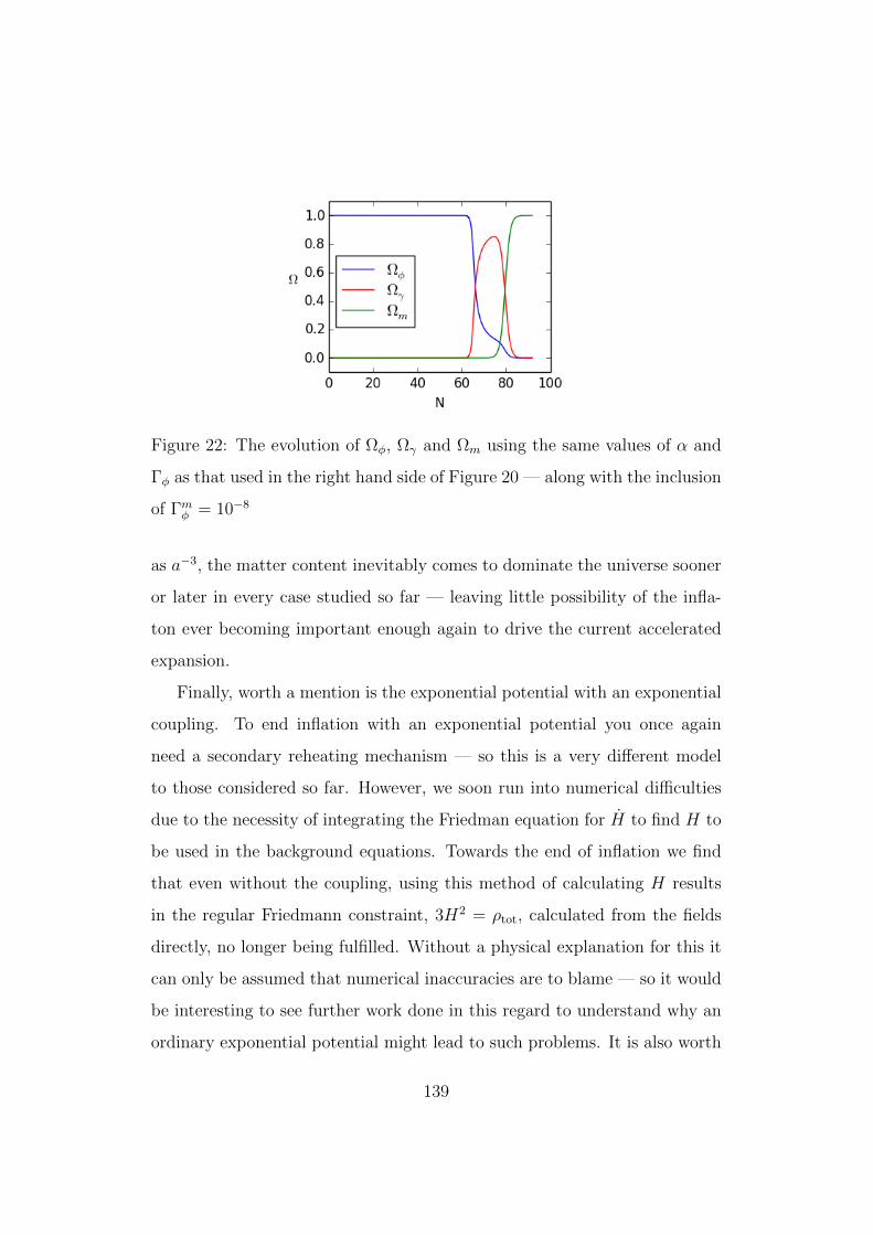
Figure 22: The evolution of Ωφ, Ωγ and Ωm using the same values of α and

Γφ as that used in the right hand side of Figure 20 — along with the inclusion

of Γmφ = 10−8

as a−3, the matter content inevitably comes to dominate the universe sooner

or later in every case studied so far — leaving little possibility of the infla-

ton ever becoming important enough again to drive the current accelerated

expansion.

Finally, worth a mention is the exponential potential with an exponential

coupling. To end inflation with an exponential potential you once again

need a secondary reheating mechanism — so this is a very different model

to those considered so far. However, we soon run into numerical difficulties

due to the necessity of integrating the Friedman equation for H to find H to

be used in the background equations. Towards the end of inflation we find

that even without the coupling, using this method of calculating H results

in the regular Friedmann constraint, 3H2 = ρtot, calculated from the fields

directly, no longer being fulfilled. Without a physical explanation for this it

can only be assumed that numerical inaccuracies are to blame — so it would

be interesting to see further work done in this regard to understand why an

ordinary exponential potential might lead to such problems. It is also worth

139

noting that this is not usually a problem, as without a Gauss-Bonnet coupling

one can calculate H from the fields to use in the background equations, but

the discrepancy must be understood in the uncoupled case in order to proceed

with the additional terms.

To summarise, a number of papers find reason to be optimistic with

some of the models considered here in terms of linking inflation to dark

energy/quintessence via a Gauss-Bonnet interaction. Most do so via an ana-

lytical approach using generalisations of behaviour such as assuming a period

of kination once inflation ends and reheating occurs or simply by introducing

a radiation component artificially. When we considered the full numerical

treatment of this with a more realistic, albeit simple method of reheating,

we have soon seen that the post-inflationary behaviour of the coupled field,

whether oscillatory or not, is much less predictable than perhaps would be

anticipated. It appears that the field loses energy due to the expansion of

space at different rates depending on the other background components —

which makes it important for future work to be done looking further into

this to understand why this is. Other avenues are also opened up via the

inclusion of different reheating mechanisms, other simple potentials and/or

couplings and further checks on whether parameters that result in realistic

post-inflationary expansion histories also align well with observational con-

straints from inflation itself [180]. Finally, it remains to be seen just how

much fine tuning is required in these models in order to find a completely

realistic description of the universe, but this can only come once the above

points are better understood.

140

A Appendix

A.1 Time dependence of the slow-roll parameters

We begin with a look at the time dependence of ε. By taking the derivative

of the usual definition (ε = −H/H2) we find that

ε = − H

H2+ 2

H2

H3, (A.1)

where H itself can be written as

H = −σσ

= 3Hσ2 + Vσσ. (A.2)

Using the expression, σ2 = 2H2ε, we can then simply express this partially

in slow-roll parameters, leaving a term ∝ Vσ/σ which can itself be expanded

(via a slightly lengthy calculation) as

Vσσ

= −3H −Hε+Hησσ +Hξ1s2θc

2θ. (A.3)

Putting all of these together, we come to the final expression:

ε = 2Hε(2ε− ησσ − ξ1s2θcθ). (A.4)

Next, we need to find the ηIJ parameters. To do this, we will need to use the

relation (found by a long winded but relatively simple bit of trigonometry),

θ = −H(ησs + ξ1sθc

2θ

), (A.5)

as it will come in handy in a good number of the efforts to find the time

derivatives. We start by differentiating the definition of ηIJ and, for clarity,

jump straight into a specific example — the isocurvature parameter ηss,

ηIJ =VIJ3H2

,

˙ηss = −2VssH

3H3+

˙Vss3H2

, (A.6)

141

The first term on the right hand side of Eq. (A.6) can easily be found via the

definition of ε just below (Eq. (1.25)) and ηIJ (Eq. (1.78)) but the second

term is slightly more challenging, requiring the use of the definition,

Vss = sin2 θVφφ − 2 sin θ cos θe−bVφχ + e−2b cos2 θVχχ. (A.7)

Differentiating this and following some algebra we arrive at

˙Vss = 2θ(−Vσs) + σ(Vσss + 2 cos2(θ)bφe

−b(sin θVφχ − cos θe−bVχχ)). (A.8)

Now, using Eq. (A.5) and expanding Eq. (A.6) using the usual slow roll

definitions, we can show that

˙ηss = 2Hεηss −Hασss

+1

3H2

[−2Vσsθ + σ

(2 cos2(θ)bφe

−b(sin θVφχ − cos θe−bVχχ))]

= 2Hεηss + 2ησs(Hησs +Hξ1sθc2θ)− 2Hc2

θsθξ1ησs − 2Hc3θξ1ηss −Hασss

= 2Hεηss + 2Hη2σs − 2Hc3

θξ1ηss −Hασss, (A.9)

where a new higher order parameter has been defined as:

αIJK ≡VσVIJKV 2

. (A.10)

Following identical working, it can also be shown that

˙ησσ = 2Hεησσ − 2Hεησs − 2Hησσξ1s2θcθ − 4Hησsξ1sθc

2θ −Hασσσ, (A.11)

˙ησs = 2Hεησs +Hησsησσ −Hησsηss − 2Hηssξ1sθc2θ −Hησsξ1cθ −Hασσs.

(A.12)

142

The equivalent first order non-canonical slow-roll parameter, ξ1, can be ex-

panded as follows for its time derivative:

ξ1 =bφε√

2ε+√

2εbφφφ

=4Hbφε

2

√2ε−√

2Hbφεησσ√ε

−√

2Hbφεξ1s2θcθ√

ε+√

2εbφφσcθ

= 2Hεξ1 −Hξ1ησσ −Hξ21s

2θcθ + 2Hεbφφcθ

= 2Hεξ1 −Hξ1ησσ −Hξ21s

2θcθ +Hξ2cθ. (A.13)

The second order non-canonical slow-roll parameter, ξ2, can be neglected

in these time derivative calculations as all time dependence will be third

order in nature — beyond what is needed here.

A.2 Evaluating f(x) and g(x)

A.2.1 f(x) — the first order function

Breaking down the asymptotic form of the Hankel functions into

H(1)µ (x) = Jµ(x) + iNµ(x), (A.14)

where Jµ(x) is the Bessel function and Nµ(x) is the Neumann function, then

the derivatives of Jµ and Nµ with respect to µ are,

dJµdµ

= −(1/2x)µ Ψ (µ+ 1)

Γ (µ+ 1)+

(x/2)µ ln (x/2)

Γ (µ+ 1),

dNµ

dµ=i (x/2)−µ Ψ (1− µ)

Γ (1− µ) sin (π µ)− i (x/2)−µ cos (π µ) π

Γ (1− µ) (sin (π µ))2 −i (x/2)−µ ln (x/2)

Γ (1− µ) sin (π µ),

(A.15)

where Ψ is the digamma function defined by

Ψ(y) =d

dyln Γ(y) =

Γ′(y)

Γ(y). (A.16)

143

We now evaluate these derivatives at µ = 3/2 to find:

dJµdµ

∣∣∣∣µ=3/2

= −√

2x3/2 (8/3− γ − 2 ln (2))

3√π

+

√2x3/2 ln (x/2)

3√π

,

dNµ

dµ

∣∣∣∣µ=3/2

=i√

2 (2− γ − 2 ln (2))√πx3/2

− i√

2 ln (x/2)√πx3/2

. (A.17)

in which we have γ which is known as the Euler-Mascheroni constant (≈

0.577). The original Hankel function also needs evaluating here, as

H(1)3/2 =

√2x3/2

3√π−√

2√πx3/2

. (A.18)

Now with the definition of f(x) in Eq. (3.69) we get,

f(x)|3/2 =− 1

3(x3 + 3i)

(8x3 − 3x3γ − 3x3 ln(2)− 3x3 ln(x)

− 18i+ 9iγ + 9i ln(2) +9i ln(x)) , (A.19)

which can be multiplied through by the conjugate of the denominator to give,

f(x) =−x3 + 3 i

3x6 + 27

(8x3 − 3x3γ − 3x3 ln (2)− 3x3 ln (x)

−18 i+ 9 iγ + 9 i ln (2) + 9 i ln (x)) , (A.20)

the real components of which are

Re[f(x)] =−8/3x6 + x6γ + x6 ln (2) + 18− 9 γ − 9 ln (2)− 9 ln (x)

x6 + 9,

(A.21)

which can be evaluated in the limit x→ 0 as,

f(x→ 0) = −γ − ln (2) + 2− ln (x) (A.22)

A.2.2 g(x) — the second order function

Following the same method, but with somewhat lengthier calculations we

can arrive at an equally necessary evaluation of g(x). Taking the second

144

derivatives of the Bessel and Neumann functions,

d2Jµdµ2

=(1/2x)µ (Ψ (µ+ 1))2

Γ (µ+ 1)− 2

(1/2x)µ ln (1/2x) Ψ (µ+ 1)

Γ (µ+ 1)

− (1/2x)µ Ψ (1, µ+ 1)

Γ (µ+ 1)+

(1/2x)µ (ln (1/2x))2

Γ (µ+ 1),

d2N2µ

dµ=i (1/2x)−µ (Ψ (1− µ))2

Γ (1− µ) sin (π µ)− 2 i (1/2x)−µ Ψ (1− µ) cos (π µ) π

Γ (1− µ) (sin (π µ))2

− 2 i (1/2x)−µ ln (1/2x) Ψ (1− µ)

Γ (1− µ) sin (π µ)− i (1/2x)−µ Ψ (1, 1− µ)

Γ (1− µ) sin (π µ)

+2 i (1/2x)−µ (cos (π µ))2 π2

Γ (1− µ) (sin (π µ))3 +2 i (1/2x)−µ ln (1/2x) cos (π µ) π

Γ (1− µ) (sin (π µ))2

+i (1/2x)−µ π2

Γ (1− µ) sin (π µ)+i (1/2x)−µ (ln (1/2x))2

Γ (1− µ) sin (π µ)(A.23)

We now evaluate these derivatives at µ = 3/2 to find:

d2Jµdµ2

∣∣∣∣µ=3/2

= −√

2x3/2

54√π

[9π2 − 18 γ2 − 36 γ ln (2)− 36 ln (x) γ − 18 (ln (2))2

−36 ln (x) ln (2)− 18 (ln (x))2 + 96 γ

+96 ln (2) + 96 ln (x)− 208]

d2Nµ

dµ2

∣∣∣∣µ=3/2

=i√

2 (2− γ − 2 ln (2))2

√πx3/2

− 2 i√

2 ln (1/2x) (2− γ − 2 ln (2))√πx3/2

− i√

2 (4 + 1/2π2)√πx3/2

+iπ3/2

√2

x3/2+i√

2 (ln (1/2x))2

√πx3/2

.

(A.24)

Lastly, we need to calculate the one component of g(x) remaining, the term

in Eq. (3.70) given by,

Re

1

H(1)3/2(x)

d2H(1)µ (x)

dµ2

∣∣∣∣∣µ=3/2

, (A.25)

145

which for the moment shall be informally denoted by H ′′/H. So the real

part, evaluated at µ = 3/2 is

H ′′

H=

−1

18x6 + 162

(−36x6γ ln (2)− 36x6 ln (x) γ − 36x6 ln (x) ln (2)− 18x6γ2

−18x6 (ln (2))2 + 9x6π2 − 18x6 (ln (x))2 − 208x6 + 96x6γ

+96x6 ln (2) + 96x6 ln (x)− 162 γ2 + 648 γ − 162 (ln (x))2

−324 ln (x) γ − 324 γ ln (2)− 162 (ln (2))2 + 648 ln (x)

+648 ln (2)− 324 ln (x) ln (2)− 81π2), (A.26)

which can be evaluated in the limit x→ 0 to give

H(x→ 0)′′

H(x→ 0)= 2 γ ln (2) + (ln (2))2 − 4 ln (2) + 1/2 π2 − 4 γ + γ2 − (ln (x))2

− 2 ln (x) γ + 4 ln (x)− 2 ln (x) ln (2) (A.27)

Now with the definition of g(x), and using some of the calculations in the

previous section — for calculating f(x), we get,

6g(x) = 16 + 24 γ ln (2) + 12 (ln (2))2 − 44 ln (2) + 3 π2 − 44 γ + 12 γ2

+ 24 ln (x) γ + 24 ln (x) ln (2)− 44 ln (x) + 12 (ln (x))2 ,

(A.28)

in which we have multiplied by 6 purely for ease of notation later on.

146

References

[1] C. van de Bruck and M. Robinson, JCAP 1408 (2014) 024

doi:10.1088/1475-7516/2014/08/024 [arXiv:1404.7806 [astro-ph.CO]].

[2] C. van de Bruck, A. J. Christopherson and M. Robinson, Phys.

Rev. D 91 (2015) 12, 123503 doi:10.1103/PhysRevD.91.123503

[arXiv:1503.06490 [astro-ph.CO]].

[3] A. Einstein, ”On the electrodynamics of moving bodies”. Annalen der

Physik 17, 891 (1905).

[4] A. Einstein, ”The Field Equations of Gravitation”. Preussische

Akademie der Wissenschaften, Sitzungsberichte, 1915 (part 2), 844847

[5] Friedmann, A. 1922, Zs. f. Phys., 10, 377.

[6] Sudbury, A., ”Quantum mechanics and the particles of nature”. Cam-

bridge University Press; Cambridge (UK) ,(1986); ISBN 0 521 25891

X.

[7] Hubble, E., ”A Relation between Distance and Radial Velocity among

Extra-Galactic Nebulae”. Proceedings of the National Academy of Sci-

ences of the United States of America, Volume 15, Issue 3, pp. 168-173,

(1929)

[8] A. G. Riess et al. [Supernova Search Team Collaboration], Astron. J.

116 (1998) 1009 doi:10.1086/300499 [astro-ph/9805201].

[9] S. Perlmutter et al. [Supernova Cosmology Project Collaboration], As-

trophys. J. 517 (1999) 565 doi:10.1086/307221 [astro-ph/9812133].

147

[10] P. A. R. Ade et al. [Planck Collaboration], arXiv:1303.5062 [astro-

ph.CO].

[11] A. A. Penzias and R. W. Wilson, Astrophys. J. 142 (1965) 419.

doi:10.1086/148307

[12] A. H. Guth, Phys. Rev. D 23 (1981) 347. doi:10.1103/PhysRevD.23.347

[13] A. D. Linde, Phys. Lett. B 108 (1982) 389. doi:10.1016/0370-

2693(82)91219-9

[14] P. A. R. Ade et al. [Planck Collaboration], arXiv:1303.5086 [astro-

ph.CO].

[15] W. Y. Wong, A. Moss and D. Scott, Mon. Not. Roy. Astron. Soc. 386,

1023 (2008) [arXiv:0711.1357 [astro-ph]].

[16] S. Seager, D. D. Sasselov and D. Scott, Astrophys. J. 523, L1 (1999)

[astro-ph/9909275].

[17] P. J. E. Peebles, Astrophys. J. 153 (1968) 1.

[18] J. C. Mather, E. S. Cheng, R. A. Shafer, C. L. Bennett, N. W. Boggess,

E. Dwek, M. G. Hauser and T. Kelsall et al., Astrophys. J. 354, L37

(1990).

[19] J. L. Puget, A. Abergel, J. P. Bernard, F. Boulanger, W. B. Burton,

F. X. Desert and D. Hartmann, Astron. Astrophys. 308 (1996) L5.

[20] G. Hinshaw et al. [WMAP Collaboration], Astrophys. J. Suppl. 148

(2003) 135 doi:10.1086/377225 [astro-ph/0302217].

[21] M. Tegmark, A. de Oliveira-Costa and A. Hamilton, Phys. Rev. D 68

(2003) 123523 doi:10.1103/PhysRevD.68.123523 [astro-ph/0302496].

148

[22] E. Komatsu et al. [WMAP Collaboration], Astrophys. J. Suppl. 192

(2011) 18 [arXiv:1001.4538 [astro-ph.CO]].

[23] J. B. Peterson, J. E. Carlstrom, E. S. Cheng, M. Kamionkowski,

A. E. Lange, M. Seiffert, D. N. Spergel and A. Stebbins, astro-

ph/9907276.

[24] J. A. Tauber , “The Planck Mission,” Advances in Space Research. 34

(2004) 3

[25] Planck Collaboration. “Planck. The Scientific Program”

http://www.rssd.esa.int/SA/PLANCK/docs/Bluebook-ESA-SCI

[26] L. P. L. Colombo, E. Pierpaoli and J. R. Pritchard, Mon. Not. Roy.

Astron. Soc. 398 (2009) 1621 [arXiv:0811.2622 [astro-ph]].

[27] P. A. R. Ade et al. [Planck Collaboration], Astron. Astrophys. 571

(2014) A22 doi:10.1051/0004-6361/201321569 [arXiv:1303.5082 [astro-

ph.CO]].

[28] P. Peter and J.-P. Uzan, Primordial Cosmology, Oxford Graduate Texts.

2009.

[29] Brustein, R. Review of Smalll Field Models of Inflation. [online] Acces-

sible at: http://hep.physics.uoc.gr/cosmo10/talks/smallfieldCRETE10

[30] A. R. Liddle and S. M. Leach, Phys. Rev. D 68 (2003) 103503 [astro-

ph/0305263].

[31] A. R. Liddle and D. H. Lyth, Cosmological Inflation and Large-Scale

Structure, Cambridge University Press, Cambridge, 2000.

149

[32] A. D. Dolgov, Phys. Rept. 222 (1992) 309. doi:10.1016/0370-

1573(92)90107-B

[33] L. F. Abbott, E. Farhi and M. B. Wise, Phys. Lett. B 117 (1982) 29.

doi:10.1016/0370-2693(82)90867-X

[34] R. Allahverdi, R. Brandenberger, F. Y. Cyr-Racine and A. Mazumdar,

Ann. Rev. Nucl. Part. Sci. 60 (2010) 27 [arXiv:1001.2600 [hep-th]].

[35] I. Huston and A. J. Christopherson, arXiv:1302.4298 [astro-ph.CO].

[36] J. H. Traschen and R. H. Brandenberger, Phys. Rev. D 42 (1990) 2491.

doi:10.1103/PhysRevD.42.2491

[37] L. Kofman, A. D. Linde and A. A. Starobinsky, Phys. Rev. Lett. 76

(1996) 1011 [hep-th/9510119].

[38] D. Boyanovsky, H. J. de Vega, R. Holman and J. F. J. Salgado, In *Paris

1996, String theory in curved space times* 260-280 [astro-ph/9609007].

[39] D. Boyanovsky, M. D’Attanasio, H. J. de Vega, R. Holman and D.-

S. Lee, Phys. Rev. D 52 (1995) 6805 [hep-ph/9507414].

[40] Baumann, D. ”Reheating after Inflation”.

http://www.damtp.cam.ac.uk/user/db275/TEACHING/INFLATION/Reheating.pdf

[accessed Mar 15].

[41] Richards, John Alan. Analysis of periodically time-varying systems.

Berlin: Springer-Verlag, 1983.

[42] Verhulst, F., 2008.Perturbation Analysis of Parametric Reso-

nance. http://www.staff.science.uu.nl/ verhu101/Parametric.pdf. [ac-

cessed Mar 15]

150

[43] D. T. Son, Phys. Rev. D 54 (1996) 3745 [hep-ph/9604340].

[44] P. R. Anderson, C. Molina-Paris, D. Evanich and G. B. Cook, Phys.

Rev. D 78 (2008) 083514 [arXiv:0801.0730 [hep-ph]].

[45] H. Kurki-Suonio, 2011. Cosmological Perturbation Theory.

Lecture course: University of Helsinki [2010]. Online at:

http://www.helsinki.fi/ hkurkisu/CosPer.pdf

[46] A. Riotto, “Inflation and the theory of cosmological perturbations,” hep-

ph/0210162.

[47] H. V. Peiris et al. [WMAP Collaboration], Astrophys. J. Suppl. 148

(2003) 213 doi:10.1086/377228 [astro-ph/0302225].

[48] P. A. R. Ade et al. [Planck Collaboration], arXiv:1502.02114 [astro-

ph.CO].

[49] Josan, A.S., “Constraints on the power spectrum of primordial pertur-

bations from small-scale structure”, Thesis - University of Nottingham

(2010)

[50] J. Lesgourgues, 2006. Inflationary Cosmology. Lecture course at

LAPTH, Annecy-Le-Vieux, France.

[51] A. Ashoorioon, C. van de Bruck, P. Millington and S. Vu, Phys. Rev. D

90 (2014) 10, 103515 [arXiv:1406.5466 [astro-ph.CO]].

[52] M. J. Mortonson and U. Seljak, JCAP 1410 (2014) 10, 035

[arXiv:1405.5857 [astro-ph.CO]].

151

[53] P. A. R. Ade et al. [BICEP2 Collaboration], Phys. Rev. Lett. 112 (2014)

24, 241101 doi:10.1103/PhysRevLett.112.241101 [arXiv:1403.3985

[astro-ph.CO]].

[54] R. Easther, J. Frazer, H. V. Peiris and L. C. Price, Phys. Rev. Lett. 112

(2014) 161302 [arXiv:1312.4035 [astro-ph.CO]].

[55] D. Wands, Lect. Notes Phys. 738 (2008) 275 [astro-ph/0702187

[ASTRO-PH]].

[56] J. Meyers and E. R. M. Tarrant, Phys. Rev. D 89 (2014) 6, 063535

[arXiv:1311.3972 [astro-ph.CO]].

[57] B. A. Bassett, S. Tsujikawa and D. Wands, Rev. Mod. Phys. 78 (2006)

537 [astro-ph/0507632].

[58] E. J. Copeland, A. R. Liddle, D. H. Lyth, E. D. Stewart and D. Wands,

Phys. Rev. D 49 (1994) 6410 [astro-ph/9401011].

[59] A. R. Liddle, A. Mazumdar and F. E. Schunck, Phys. Rev. D 58 (1998)

061301 [astro-ph/9804177].

[60] C. Gordon, D. Wands, B. A. Bassett and R. Maartens, Phys. Rev. D 63

(2001) 023506 doi:10.1103/PhysRevD.63.023506 [astro-ph/0009131].

[61] S. Groot Nibbelink and B. J. W. van Tent, Class. Quant. Grav. 19

(2002) 613 [hep-ph/0107272].

[62] S. A. Kim and A. R. Liddle, Phys. Rev. D 74 (2006) 023513 [astro-

ph/0605604].

[63] M. Grana, Phys. Rept. 423 (2006) 91 [hep-th/0509003].

152

[64] F. Denef, M. R. Douglas and S. Kachru, Ann. Rev. Nucl. Part. Sci. 57

(2007) 119 [hep-th/0701050].

[65] G. Shiu and J. Xu, Phys. Rev. D 84, 103509 (2011) [arXiv:1108.0981

[hep-th]].

[66] A. Avgoustidis, S. Cremonini, A. C. Davis, R. H. Ribeiro, K. Turzynski

and S. Watson, JCAP 1202, 038 (2012) [arXiv:1110.4081 [astro-ph.CO]].

[67] C. Gordon, D. Wands, B. A. Bassett and R. Maartens, Phys. Rev. D 63

(2001) 023506 [astro-ph/0009131].

[68] F. Di Marco, F. Finelli and R. Brandenberger, Phys. Rev. D 67 (2003)

063512 [astro-ph/0211276].

[69] Z. Lalak, D. Langlois, S. Pokorski and K. Turzynski, JCAP 0707 (2007)

014 [arXiv:0704.0212 [hep-th]].

[70] D. H. Lyth and D. Wands, Phys. Lett. B 524 (2002) 5 [hep-ph/0110002].

[71] N. Bartolo and A. R. Liddle, Phys. Rev. D 65 (2002) 121301 [astro-

ph/0203076].

[72] K. Enqvist, R. N. Lerner and O. Taanila, JCAP 1112 (2011) 016

[arXiv:1105.0498 [astro-ph.CO]].

[73] C. T. Byrnes, M. Corts and A. R. Liddle, Phys. Rev. D 90 (2014) 2,

023523 [arXiv:1403.4591 [astro-ph.CO]].

[74] D. Langlois and F. Vernizzi, Phys. Rev. D 70 (2004) 063522 [astro-

ph/0403258].

[75] K. Dimopoulos, K. Kohri, D. H. Lyth and T. Matsuda, JCAP 1203

(2012) 022 [arXiv:1110.2951 [astro-ph.CO]].

153

[76] T. Moroi, T. Takahashi and Y. Toyoda, Phys. Rev. D 72 (2005) 023502

[hep-ph/0501007].

[77] V. F. Mukhanov and P. J. Steinhardt, Phys. Lett. B 422 (1998) 52

[astro-ph/9710038].

[78] F. Di Marco and F. Finelli, Phys. Rev. D 71 (2005) 123502 [astro-

ph/0505198].

[79] K. Y. Choi, L. M. H. Hall and C. van de Bruck, JCAP 0702 (2007) 029

[astro-ph/0701247].

[80] J. Lachapelle and R. H. Brandenberger, JCAP 0904 (2009) 020

[arXiv:0808.0936 [hep-th]].

[81] Jordan, Pascual. ”Formation of the Stars and Development of the Uni-

verse.” Nature 164.4172 (1949): 637-640.

[82] Brans, Carl, and Robert H. Dicke. ”Mach’s principle and a relativistic

theory of gravitation.” Physical Review 124.3 (1961): 925.

[83] V. Faraoni, Phys. Rev. D 53 (1996) 6813 [astro-ph/9602111].

[84] M. P. Hertzberg, JHEP 1011 (2010) 023 [arXiv:1002.2995 [hep-ph]].

[85] A. A. Starobinsky, S. Tsujikawa and J. Yokoyama, Nucl. Phys. B 610

(2001) 383 [astro-ph/0107555].

[86] D. I. Kaiser and A. T. Todhunter, Phys. Rev. D 81 (2010) 124037

[arXiv:1004.3805 [astro-ph.CO]].

[87] Y. Fujii and K. Maeda, The Scalar-Tensor Theory of Gravitation (New

York: Cambridge University Press, 2003

154

[88] D. I. Kaiser, Phys. Rev. D 81 (2010) 084044 [arXiv:1003.1159 [gr-qc]].

[89] P. Peter, arXiv:1303.2509 [astro-ph.CO].

[90] Christopherson, A. J., 2011. Applications of Cosmological Perturbation

Theory [Thesis]. http://arxiv.org/abs/1106.0446

[91] C. Uggla and J. Wainwright, Gen. Rel. Grav. 45 (2013) 643

[arXiv:1203.4790 [astro-ph.CO]].

[92] K. Nakamura, Adv. Astron. 2010 (2010) 576273 [arXiv:1001.2621 [gr-

qc]].

[93] Durrer, R., 2004. Cosmological Perturbation Theory.

http://theory.physics.unige.ch/ durrer/courses/syros.pdf

[94] V. Acquaviva, N. Bartolo, S. Matarrese and A. Riotto, Nucl. Phys. B

667 (2003) 119 [astro-ph/0209156].

[95] Kodama, Hideo, and Misao Sasaki. ”Cosmological perturbation theory.”

Progress of Theoretical Physics Supplement 78 (1984): 1-166.

[96] K. A. Malik and D. Wands, Class. Quant. Grav. 21 (2004) L65 [astro-

ph/0307055].

[97] A. J. Christopherson, K. A. Malik and D. R. Matravers, Phys. Rev. D

83 (2011) 123512 [arXiv:1008.4866 [astro-ph.CO]].

[98] Mukhanov, Viatcheslav F., Hume A. Feldman, and Robert Hans Bran-

denberger. ”Theory of cosmological perturbations.” Physics Reports

215.5 (1992): 203-333.

155

[99] C. Baccigalupi, 2015. Linear Cosmological Perturbations and Cosmic

Microwave Background Anisotropies [Lectures: SISSA, Trieste, Italy].

Available online at: http://people.sissa.it/ bacci/work/lectures/SISSA,

[100] J. M. Bardeen, Phys. Rev. D 22 (1980) 1882.

[101] J. c. Hwang and H. Noh, Phys. Lett. B 495 (2000) 277

doi:10.1016/S0370-2693(00)01253-3 [astro-ph/0009268].

[102] J. C. Hwang and H. Noh, Phys. Rev. D 73 (2006) 044021

doi:10.1103/PhysRevD.73.044021 [astro-ph/0601041].

[103] D. Langlois and S. Renaux-Petel, JCAP 0804 (2008) 017

[arXiv:0801.1085 [hep-th]].

[104] D. Wands, K. A. Malik, D. H. Lyth and A. R. Liddle, Phys. Rev. D

62 (2000) 043527 [astro-ph/0003278].

[105] K. A. Malik and D. Wands, Phys. Rept. 475 (2009) 1 [arXiv:0809.4944

[astro-ph]].

[106] D. H. Lyth, C. Ungarelli and D. Wands, Phys. Rev. D 67 (2003) 023503

[astro-ph/0208055].

[107] K. Enqvist and T. Takahashi, JCAP 1310 (2013) 034 [arXiv:1306.5958

[astro-ph.CO]].

[108] J. Fonseca and D. Wands, JCAP 1206 (2012) 028 [arXiv:1204.3443

[astro-ph.CO]].

[109] D. Wands, N. Bartolo, S. Matarrese and A. Riotto, Phys. Rev. D 66

(2002) 043520 [astro-ph/0205253].

156

[110] K. Enqvist, S. Nurmi and G. I. Rigopoulos, JCAP 0810 (2008) 013

[arXiv:0807.0382 [astro-ph]].

[111] K. Enqvist, D. G. Figueroa and R. N. Lerner, JCAP 1301 (2013) 040

[arXiv:1211.5028 [astro-ph.CO]].

[112] T. Markkanen and A. Tranberg, JCAP 1211 (2012) 027

[arXiv:1207.2179 [gr-qc]].

[113] S. Tsujikawa, D. Parkinson and B. A. Bassett, Phys. Rev. D 67 (2003)

083516 [astro-ph/0210322].

[114] C. T. Byrnes, K. Y. Choi and L. M. H. Hall, JCAP 0810 (2008) 008

[arXiv:0807.1101 [astro-ph]].

[115] J. Elliston, D. J. Mulryne, D. Seery and R. Tavakol, JCAP 1111 (2011)

005 [arXiv:1106.2153 [astro-ph.CO]].

[116] S. Cremonini, Z. Lalak and K. Turzynski, Phys. Rev. D 82 (2010)

047301 [arXiv:1005.4347 [hep-th]].

[117] J. Garcia-Bellido and D. Wands, Phys. Rev. D 52, 6739 (1995) [gr-

qc/9506050].

[118] A. A. Starobinsky and J. Yokoyama, gr-qc/9502002.

[119] D. Wands, K. A. Malik, D. H. Lyth and A. R. Liddle, Phys. Rev. D

62 (2000) 043527 doi:10.1103/PhysRevD.62.043527 [astro-ph/0003278].

[120] Kofman, L. A. and Linde, A. D., Generation of density perturbations

in inflationary cosmology, Nuclear Phys. B 282 (1987) 555–588.

[121] D. Wands and J. Garcia-Bellido, Helv. Phys. Acta 69 (1996) 211 [astro-

ph/9608042].

157

[122] D. Langlois, Phys. Rev. D 59 (1999) 123512

doi:10.1103/PhysRevD.59.123512 [astro-ph/9906080].

[123] N. Bartolo, S. Matarrese and A. Riotto, Phys. Rev. D 64 (2001) 083514

doi:10.1103/PhysRevD.64.083514 [astro-ph/0106022].

[124] C. T. Byrnes and D. Wands, Phys. Rev. D 74 (2006) 043529

doi:10.1103/PhysRevD.74.043529 [astro-ph/0605679].

[125] S. Cremonini, Z. Lalak and K. Turzynski, JCAP 1103 (2011) 016

doi:10.1088/1475-7516/2011/03/016 [arXiv:1010.3021 [hep-th]].

[126] W. Hu, Phys. Rev. D 84 (2011) 027303

doi:10.1103/PhysRevD.84.027303 [arXiv:1104.4500 [astro-ph.CO]].

[127] Starobinsky, A., Multicomponent de Sitter (Inflationary) Stages and

the Generation of Perturbations, JETP Lett. 42 (1985). 152-155.

[128] M. Sasaki and E. D. Stewart, Prog. Theor. Phys. 95 (1996) 71

doi:10.1143/PTP.95.71 [astro-ph/9507001].

[129] H. C. Lee, M. Sasaki, E. D. Stewart, T. Tanaka and S. Yokoyama,

JCAP 0510 (2005) 004 doi:10.1088/1475-7516/2005/10/004 [astro-

ph/0506262].

[130] N. S. Sugiyama, E. Komatsu and T. Futamase, Phys. Rev. D 87 (2013)

2, 023530 doi:10.1103/PhysRevD.87.023530 [arXiv:1208.1073 [gr-qc]].

[131] R. N. Greenwood, D. I. Kaiser and E. I. Sfakianakis, Phys. Rev. D 87,

no. 6, 064021 (2013) [arXiv:1210.8190 [hep-ph]].

[132] D. I. Kaiser, E. A. Mazenc and E. I. Sfakianakis, Phys. Rev. D 87, no.

6, 064004 (2013) [arXiv:1210.7487 [astro-ph.CO]].

158

[133] D. I. Kaiser and E. I. Sfakianakis, Phys. Rev. Lett. 112, 011302 (2014)

[arXiv:1304.0363 [astro-ph.CO]].

[134] J. White, M. Minamitsuji and M. Sasaki, JCAP 1207 (2012) 039

[arXiv:1205.0656 [astro-ph.CO]]

[135] J. Garriga and V. F. Mukhanov, Phys. Lett. B 458 (1999) 219 [hep-

th/9904176].

[136] R. Gwyn, M. Rummel and A. Westphal, JCAP 1312 (2013) 010

[arXiv:1212.4135 [hep-th]].

[137] X. Chen, M. x. Huang, S. Kachru and G. Shiu, JCAP 0701 (2007) 002

[hep-th/0605045].

[138] P. Franche, R. Gwyn, B. Underwood and A. Wissanji, Phys. Rev. D

81 (2010) 123526 [arXiv:0912.1857 [hep-th]].

[139] Makino, Nobuyoshi, and Misao Sasaki. ”The density perturbation in

the chaotic inflation with non-minimal coupling.” Progress of Theoreti-

cal Physics 86.1 (1991): 103-118.

[140] C. van de Bruck and L. E. Paduraru, Phys. Rev. D 92 (2015) 8, 083513

doi:10.1103/PhysRevD.92.083513 [arXiv:1505.01727 [hep-th]].

[141] Sasaki, M., Large Scale Quantum Fluctuations in the Inflationary Uni-

verse, Prog. Theor. Phys. 76.

[142] Mukhanov, V., Quantum theory of gauge-invariant cosmological per-

turbations, Sov. Phys. JETP 67.

[143] C. Gordon and P. M. Saffin, JCAP 1308 (2013) 021 doi:10.1088/1475-

7516/2013/08/021 [arXiv:1304.5229 [hep-th]].

159

[144] A. Ashoorioon, H. Firouzjahi and M. M. Sheikh-Jabbari, JCAP 1005

(2010) 002 doi:10.1088/1475-7516/2010/05/002 [arXiv:0911.4284 [hep-

th]].

[145] H. Kodama, K. Kohri and K. Nakayama, Prog. Theor. Phys. 126

(2011) 331 doi:10.1143/PTP.126.331 [arXiv:1102.5612 [astro-ph.CO]].

[146] S. Clesse, Phys. Rev. D 83 (2011) 063518

doi:10.1103/PhysRevD.83.063518 [arXiv:1006.4522 [gr-qc]].

[147] A. A. Abolhasani, H. Firouzjahi and M. H. Namjoo, Class.

Quant. Grav. 28 (2011) 075009 doi:10.1088/0264-9381/28/7/075009

[arXiv:1010.6292 [astro-ph.CO]].

[148] T. S. Bunch and P. C. W. Davies, Proc. Roy. Soc. Lond. A 360 (1978)

117. doi:10.1098/rspa.1978.0060

[149] C. M. Will, Living Rev. Rel. 17 (2014) 4 [arXiv:1403.7377 [gr-qc]].

[150] P. J. Mohr, B. N. Taylor and D. B. Newell, Rev. Mod. Phys. 84 (2012)

1527 doi:10.1103/RevModPhys.84.1527 [arXiv:1203.5425 [physics.atom-

ph]].

[151] T. Moroi and T. Takahashi, Phys. Lett. B 522 (2001) 215 [Erratum-

ibid. B 539 (2002) 303] [hep-ph/0110096].

[152] P. J. Steinhardt and C. M. Will, Phys. Rev. D 52 (1995) 628 [astro-

ph/9409041].

[153] L. Perivolaropoulos and C. Sourdis, Phys. Rev. D 66 (2002) 084018

[hep-ph/0204155].

160

[154] J. Martin, C. Ringeval and V. Vennin, Phys. Dark Univ. (2014)

[arXiv:1303.3787 [astro-ph.CO]].

[155] A. R. Liddle and D. H. Lyth, Cambridge, UK: Univ. Pr. (2000) 400 p

[156] K. A. Malik and D. Wands, JCAP 0502 (2005) 007 [astro-ph/0411703].

[157] G. I. Rigopoulos and E. P. S. Shellard, Phys. Rev. D 68 (2003) 123518

[astro-ph/0306620].

[158] A. J. Christopherson and K. A. Malik, Phys. Lett. B 675 (2009) 159

[arXiv:0809.3518 [astro-ph]].

[159] J. Garcia-Bellido and D. Wands, Phys. Rev. D 53 (1996) 5437 [astro-

ph/9511029].

[160] B. A. Bassett, D. I. Kaiser and R. Maartens, Phys. Lett. B 455 (1999)

84 [hep-ph/9808404].

[161] B. A. Bassett, F. Tamburini, D. I. Kaiser and R. Maartens, Nucl. Phys.

B 561, 188 (1999) [hep-ph/9901319].

[162] B. A. Bassett, C. Gordon, R. Maartens and D. I. Kaiser, Phys. Rev. D

61 (2000) 061302 [hep-ph/9909482].

[163] I. Huston and A. J. Christopherson, Phys. Rev. D 85 (2012) 063507

[arXiv:1111.6919 [astro-ph.CO]].

[164] Z. K. Guo and D. J. Schwarz, Phys. Rev. D 80, 063523 (2009)

[arXiv:0907.0427 [hep-th]].

[165] I. Antoniadis, J. Rizos and K. Tamvakis, Nucl. Phys. B 415 (1994) 497

[hep-th/9305025].

161

[166] B. M. N. Carter and I. P. Neupane, JCAP 0606 (2006) 004 [hep-

th/0512262].

[167] E. J. Chun, S. Scopel and I. Zaballa, JCAP 0907 (2009) 022

[arXiv:0904.0675 [hep-ph]].

[168] Z. K. Guo and D. J. Schwarz, Phys. Rev. D 81 (2010) 123520

[arXiv:1001.1897 [hep-th]].

[169] K. Dimopoulos and J. W. F. Valle, Astropart. Phys. 18 (2002) 287

[astro-ph/0111417].

[170] K. Dimopoulos and J. W. F. Valle, Astropart. Phys. 18 (2002) 287

doi:10.1016/S0927-6505(02)00115-9 [astro-ph/0111417].

[171] C. Pallis, Nucl. Phys. B 751 (2006) 129 [hep-ph/0510234].

[172] H. Tashiro, T. Chiba and M. Sasaki, Class. Quant. Grav. 21 (2004)

1761 [gr-qc/0307068].

[173] G. N. Felder, L. Kofman and A. D. Linde, Phys. Rev. D 60 (1999)

103505 [hep-ph/9903350].

[174] A. H. Campos, H. C. Reis and R. Rosenfeld, Phys. Lett. B 575 (2003)

151 [hep-ph/0210152].

[175] G. N. Felder, L. Kofman and A. D. Linde, Phys. Rev. D 59 (1999)

123523 [hep-ph/9812289].

[176] P. X. Jiang, J. W. Hu and Z. K. Guo, Phys. Rev. D 88 (2013) 123508

[arXiv:1310.5579 [hep-th]].

[177] T. Koivisto and D. F. Mota, Phys. Rev. D 75 (2007) 023518 [hep-

th/0609155].

162

[178] R. Bean, S. H. Hansen and A. Melchiorri, Phys. Rev. D 64 (2001)

103508 [astro-ph/0104162].

[179] E. J. Copeland, M. Sami and S. Tsujikawa, Int. J. Mod. Phys. D 15

(2006) 1753 [hep-th/0603057].

[180] S. Koh, B. H. Lee, W. Lee and G. Tumurtushaa, Phys. Rev. D 90

(2014) 6, 063527 [arXiv:1404.6096 [gr-qc]].

163