Embed Size (px)
Citation preview
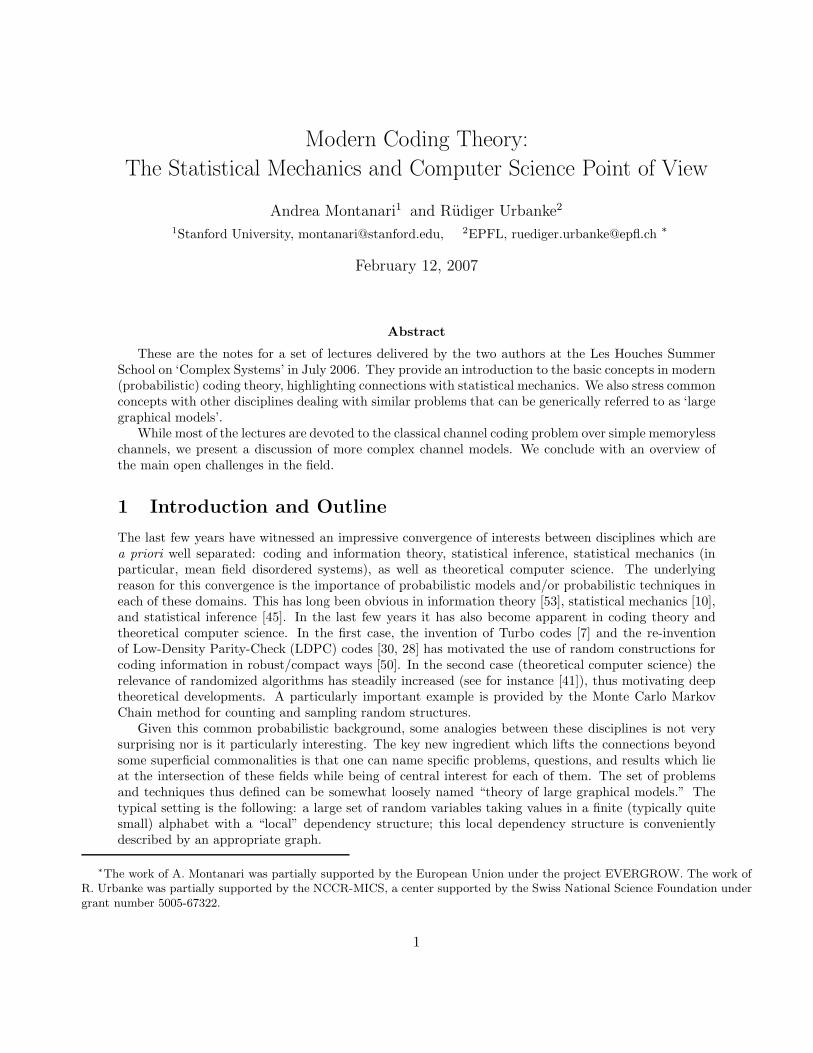
Modern Coding Theory:
The Statistical Mechanics and Computer Science Point of View
Andrea Montanari1 and Rudiger Urbanke2
1Stanford University, [email protected], 2EPFL, [email protected] ∗
February 12, 2007
Abstract
These are the notes for a set of lectures delivered by the two authors at the Les Houches SummerSchool on ‘Complex Systems’ in July 2006. They provide an introduction to the basic concepts in modern(probabilistic) coding theory, highlighting connections with statistical mechanics. We also stress commonconcepts with other disciplines dealing with similar problems that can be generically referred to as ‘largegraphical models’.
While most of the lectures are devoted to the classical channel coding problem over simple memorylesschannels, we present a discussion of more complex channel models. We conclude with an overview ofthe main open challenges in the field.
1 Introduction and Outline
The last few years have witnessed an impressive convergence of interests between disciplines which area priori well separated: coding and information theory, statistical inference, statistical mechanics (inparticular, mean field disordered systems), as well as theoretical computer science. The underlyingreason for this convergence is the importance of probabilistic models and/or probabilistic techniques ineach of these domains. This has long been obvious in information theory [53], statistical mechanics [10],and statistical inference [45]. In the last few years it has also become apparent in coding theory andtheoretical computer science. In the first case, the invention of Turbo codes [7] and the re-inventionof Low-Density Parity-Check (LDPC) codes [30, 28] has motivated the use of random constructions forcoding information in robust/compact ways [50]. In the second case (theoretical computer science) therelevance of randomized algorithms has steadily increased (see for instance [41]), thus motivating deeptheoretical developments. A particularly important example is provided by the Monte Carlo MarkovChain method for counting and sampling random structures.
Given this common probabilistic background, some analogies between these disciplines is not verysurprising nor is it particularly interesting. The key new ingredient which lifts the connections beyondsome superficial commonalities is that one can name specific problems, questions, and results which lieat the intersection of these fields while being of central interest for each of them. The set of problemsand techniques thus defined can be somewhat loosely named “theory of large graphical models.” Thetypical setting is the following: a large set of random variables taking values in a finite (typically quitesmall) alphabet with a “local” dependency structure; this local dependency structure is convenientlydescribed by an appropriate graph.
∗The work of A. Montanari was partially supported by the European Union under the project EVERGROW. The work ofR. Urbanke was partially supported by the NCCR-MICS, a center supported by the Swiss National Science Foundation undergrant number 5005-67322.
1

In this lecture we shall use “modern” coding theory as an entry point to the domain. There are severalmotivations for this: (i) theoretical work on this topic is strongly motivated by concrete and well-definedpractical applications; (ii) the probabilistic approach mentioned above has been quite successful and hassubstantially changed the field (whence the reference to modern coding theory); (iii) a sufficientlydetailed picture exists illustrating the interplay among different view points.
We start in Section 2 with a brief outline of the (channel coding) problem. This allows us to introducethe standard definitions and terminology used in this field. In Section 3 we introduce ensembles ofcodes defined by sparse random graphs and discuss their most basic property – the weight distribution.In Section 4 we phrase the decoding problem as an inference problem on a graph and consider theperformance of the efficient (albeit in general suboptimal) message-passing decoder. We show how theperformance of such a combination (sparse graph code and message-passing decoding) can be analyzedand we discuss the relationship of the performance under message-passing decoding to the performanceof the optimal decoder. In Section 5 we briefly touch on some problems beyond coding, in order toshow as similar concept emerge there. In particular, we discuss how message passing techniques can besuccessfully used in some families of counting/inference problems. In Section 6 we show that several ofthe simplifying assumptions (binary case, symmetry of channel, memoryless channels) are convenient inthat they allow for a simple theory but are not really necessary. In particular, we discuss a simple channelwith memory and we see how to proceed in the asymmetric case. Finally, we conclude in Section 7 witha few fundamental open problems.
To readers who would like to find current contributions on this topic we recommend the IEEETransactions on Information Theory. A considerably more in-depth discussion can be found in the twoupcoming books Information, Physics and Computation [36] and Modern Coding Theory [50]. Standardreferences on coding theory are [6, 9, 26] and very readable introductions to information theory can befound in [12, 20]. Other useful reference sources are the book by Nishimori [44] as well as the book byMacKay [29].
2 Background: The Channel Coding Problem
The central problem of communications is how to transmit information reliably through a noisy (andthus unreliable) communication channel. Coding theory aims at accomplishing this task by adding aproperly designed redundancy to the transmitted message. This redundancy is then used at the receiverto reconstruct the original message despite the noise introduced by the channel.
2.1 The Problem
In order to model the situation described above we shall assume that the noise is random with someknown distribution.1 To keep things simple we shall assume that the communication channel admits asinput binary symbols x ∈ {0, 1}, while the output belongs to some finite alphabet A. We denote theprobability of observing the output y ∈ A given that the input was x ∈ {0, 1} by Q(y|x). The channelmodel is defined by the transition probability matrix
Q = {Q(y|x) : x ∈ {0, 1}, y ∈ A} . (2.1)
Of course, the entries of this matrix must be non-negative and normalized in such a way that∑
y Q(y|x) =1. It is convenient to have a few simple examples in mind. We refer to Fig. 1 for an illustration of thechannel models which we introduce in the following three examples.
Example 1: The binary symmetric channel BSC(p) is defined by letting A = {0, 1} and Q(0|0) =Q(1|1) = 1−p; the normalization then enforces Q(1|0) = Q(0|1) = p. In words, the channel “flips”the input bit with probability p ∈ [0, 1]. Since flips are introduced for each bit independently we
1It is worth mentioning that an alternative approach would be to consider the noise as ‘adversarial’ (or worst case) undersome constraint on its intensity.
2

0 0
11
1−p
1−p
p
p
1−p
p
p
1−p00
11
*
0 0
111−p
1
p
Figure 1: Schematic description of three simple binary memoryless channels. From left to right: binarysymmetric channel BSC(p), binary erasure channel BEC(ǫ), and Z channel ZC(p).
say that the channel is memoryless. Except for an example in Section 6.2 all channels which weconsider are memoryless.
Example 2: The binary erasure channel BEC(ǫ) is defined by A = {0, 1, ∗} and Q(0|0) = Q(1|1) =1 − ǫ while Q(∗|0) = Q(∗|1) = ǫ. In words, the channel input is erased with probability ǫ and it istransmitted correctly otherwise.
Example 3: The Z-channel ZC(p) has an output alphabet A = {0, 1} but acts differently on input0 (that is transmitted correctly) and 1 (that is flipped with probability p). We invite the readerto write the transition probability matrix.
Since in each case the input is binary we speak of a binary-input channel. Since further in all models eachinput symbol is distorted independently from all other ones we say that the channels are memoryless.It is convenient to further restrict our attention to symmetric channels: this means that there is aninvolution on A (i.e. a mapping ι : A → A such that ι ◦ ι = 1) so that Q(y|0) = Q(ι(y)|1). (E.g.,if A = R then we could require that Q(y|0) = Q(−y|1).) This condition is satisfied by the first twoexamples above but not by the third one. To summarize these three properties one refers to such modelsas BMS channels.
In order to complete the problem description we need to formalize the information which is tobe transmitted. We shall model this probabilistically as well and assume that the transmitter hasan information source that provides an infinite stream of i.i.d. fair coins: {zi; i = 0, 1, 2, . . .}, withzi ∈ {0, 1} uniformly at random. The goal is to reproduce this stream faithfully after communicating itover the noisy channel.
Let us stress that, despite its simplification, the present setting contains most of the crucial andchallenges of the channel coding problem. Some of the many generalizations are described in Section 6.
2.2 Block Coding
The (general) coding strategy we shall consider here is block coding. It works as follows:
• The source stream {zi} is chopped into blocks of length L. Denote one such block by z, z =(z1, . . . , zL) ∈ {0, 1}L.
• Each block is fed into an encoder. This is a map F : {0, 1}L → {0, 1}N , for some fixed N > L (theblocklength). In words, the encoder introduces redundancy in the source message. Without loss ofgenerality we can assume F to be injective. It this was not the case, even in the absence of noise,we could not uniquely recover the transmitted information from the observed codeword.
• The image of {0, 1}L under the map F is called the codebook, or sometimes the code, and it willbe denoted by C. The code contains |C| = 2L strings of length N called codewords. These are thepossible channel inputs. The codeword x = F(z) is sent through the channel, bit by bit.
3
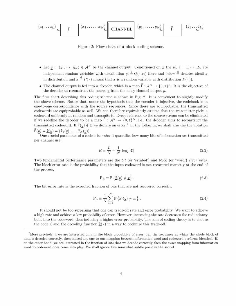
F CHANNEL F(z1 . . . zL) (x1 . . . . . . xN ) (y1 . . . . . . yN ) (z1 . . . zL)
Figure 2: Flow chart of a block coding scheme.
• Let y = (y1, · · · , yN) ∈ AN be the channel output. Conditioned on x the yi, i = 1, · · · , L, are
independent random variables with distribution yid= Q(· |xi) (here and below
d= denotes identity
in distribution and xd= P ( · ) means that x is a random variable with distribution P ( · )).
• The channel output is fed into a decoder, which is a map F : AN → {0, 1}L. It is the objective ofthe decoder to reconstruct the source z from the noisy channel output y.
The flow chart describing this coding scheme is shown in Fig. 2. It is convenient to slightly modifythe above scheme. Notice that, under the hypothesis that the encoder is injective, the codebook is inone-to-one correspondence with the source sequences. Since these are equiprobable, the transmittedcodewords are equiprobable as well. We can therefore equivalently assume that the transmitter picks acodeword uniformly at random and transmits it. Every reference to the source stream can be eliminatedif we redefine the decoder to be a map F : AN → {0, 1}N , i.e., the decoder aims to reconstruct the
transmitted codeword. If F(y) 6∈ C we declare an error.2 In the following we shall also use the notation
F(y) = x(y) = (x1(y), . . . , xN (y)).One crucial parameter of a code is its rate: it quantifies how many bits of information are transmitted
per channel use,
R ≡ L
N=
1
Nlog2 |C| . (2.2)
Two fundamental performance parameters are the bit (or ‘symbol’) and block (or ‘word’) error rates.The block error rate is the probability that the input codeword is not recovered correctly at the end ofthe process,
PB ≡ P{x(y) 6= x
}. (2.3)
The bit error rate is the expected fraction of bits that are not recovered correctly,
Pb ≡ 1
N
N∑
i=1
P{xi(y) 6= xi
}. (2.4)
It should not be too surprising that one can trade-off rate and error probability. We want to achievea high rate and achieve a low probability of error. However, increasing the rate decreases the redundancybuilt into the codeword, thus inducing a higher error probability. The aim of coding theory is to choosethe code C and the decoding function x( · ) in a way to optimize this trade-off.
2More precisely, if we are interested only in the block probability of error, i.e., the frequency at which the whole block ofdata is decoded correctly, then indeed any one-to-one mapping between information word and codeword performs identical. If,on the other hand, we are interested in the fraction of bits that we decode correctly then the exact mapping from informationword to codeword does come into play. We shall ignore this somewhat subtle point in the sequel.
4

2.3 Decoding
Given the code there is a simple (although in general not computationally efficient) prescription for thedecoder. If we want to minimize the block error rate, we must chose the most likely codeword,
xB(y) ≡ argmaxx
P{X = x|Y = y} . (2.5)
To minimize the bit error rate we must instead return the sequence of most likely bits,
xbi (y) ≡ arg max
xi
P{Xi = xi|Y = y} . (2.6)
The reason of these prescriptions is the object of the next exercise.
Exercise 1: Let (U, V ) be a pair of discrete random variables. Think of U as a ‘hidden’ variableand imagine you observe V = v. We want to understand what is the optimal estimate for U givenV = v. Show that the function v 7→ u(v) that minimizes the error probability P(u) ≡ P {U 6= u(V )}is given by
u(v) = argmaxu
P {U = u|V = v} . (2.7)
It is instructive to explicitly write down the conditional distribution of the channel input given theoutput. We shall denote it as µC,y(x) = P{X = x|Y = y} (and sometimes drop the subscripts C and yif they are clear from the context). Using Bayes rule we get
µC,y(x) =1
Z(C, y)
N∏
i=1
Q(yi|xi) IC(x) , (2.8)
where IC(x) denotes the code membership function (IC(x) = 1 if x ∈ C and = 0 otherwise).According to the above discussion, decoding amounts to computing the marginals (for symbol MAP)
or the mode3 (for word MAP) of µ( · ). More generally, we would like to understand the properties ofµ( · ): is it concentrated on a single codeword or spread over many of them? In the latter case, are theseclose to each other or very different? And what is their relationship with the transmitted codeword?
The connection to statistical mechanics emerges in the study of the decoding problem [56, 51]. Tomake it completely transparent we rewrite the distribution µ( · ) in Boltzmann form
µC,y(x) =1
Z(C, y)e−EC,y(x) , (2.9)
EC,y(x) =
{−∑N
i=1 logQ(yi|xi), if x ∈ C ,+∞, otherwise .
(2.10)
The word MAP and bit MAP rule can then be written as
xB(y) = arg minxEC,y(x) , (2.11)
xbi (y) = arg max
xi
∑
xj :j 6=i
µC,y(x) . (2.12)
In words, word MAP amounts to computing the ground state of a certain energy function, and bitMAP corresponds to computing the expectation with respect to the Boltzmann distribution. Noticefurthermore that µ( · ) is itself random because of the randomness in y (and we shall introduce furtherrandomness in the choice of the code). This is analogous to what happens in statistical physics ofdisordered systems, with y playing the role of quenched random variables.
3We recall that the mode of a distribution with density µ( · ) is the value of x that maximizes µ(x).
5

2.4 Conditional Entropy and Free Energy
As mentioned above, we are interested in understanding the properties of the (random) distributionµC,y( · ). One possible way of formalizing this idea is to consider the entropy of this distribution.
Let us recall that the (Shannon) entropy of a discrete random variable X (or, equivalently, of itsdistribution) quantifies, in a very precise sense, the ‘uncertainty’ associated with X .4 It is given by
H(X) = −∑
x
P(x) log P(x) . (2.13)
For two random variables X and Y one defines the conditional entropy of X given Y as
H(X |Y ) = −∑
x,y
P(x, y) log P(x|y) = Ey
{−∑
x
P(x|Y ) log P(x|Y )
}. (2.14)
This quantifies the remaining uncertainty about X when Y is observed.Considering now the coding problem. Denote by X the (uniformly random) transmitted codeword
and by Y the channel output. The right-most expression in Eq. (2.14) states that H(X|Y ) is theexpectation of the entropy of the conditional distribution µC,y( · ) with respect to y.
Let us denote by νC(x) the probability that a uniformly random codeword in C takes the value x atthe i-th position, averaged over i. Then a straightforward calculation yields
H(X|Y ) = − 1
|C|∑
x,y
N∏
i=1
Q(yi|xi) log
{1
Z(C, y)
N∏
i=1
Q(yi|xi)
}, (2.15)
= −N∑
x,y
νC(x)Q(y|x) logQ(y|x) + Ey logZ(C, y) . (2.16)
The ‘type’ νC(x) is usually a fairly straightforward characteristic of the code. For most of the examplesconsidered below we can take νC(0) = νC(1) = 1/2. As a consequence the first of the terms above istrivial to compute (it requires summing over 2|A| terms).
On the other hand the second term is highly non-trivial. The reader will recognize the expectationof a free energy, with y playing the role of a quenched random variable.
The conditional entropyH(X|Y ) provides an answer to the question: how many codewords is µC,y( · )spread over? It turns out that about eH(X|Y ) of them carry most of the weight.
2.5 Shannon Theorem and Random Coding
As mentioned above, there exists an obvious tradeoff between high rate and low error probability. In hiscelebrated 1948 paper [53], Shannon derived the optimal error probability-vs-rate curve in the limit oflarge blocklengths. In particular, he proved that if the rate is larger than a particular threshold, thenthe error probability can be made arbitrarily small. The threshold depends on the channel and it iscalled the channel capacity. The capacity of a BMS channel (measured in bits per channel use) is givenby the following elementary expression,
C(Q) =H(X) −H(X |Y )
=1 +∑
y
Q(y|0) log2
{Q(y|0)
Q(y|0) +Q(y|1)
}.
For instance, the capacity of a BSC(p) is C(p) = 1−h2(p), (where h2(p) = −p log2 p−(1−p) log2(1−p) isthe entropy of a Bernoulli random variable of parameter p) while the capacity of a BEC(ǫ) is C(ǫ) = 1−ǫ.As an illustration, the capacity of a BSC(p) with flip probability p ≈ 0.110028 is C(p) = 1/2: such achannel can be used to transmit reliably 1/2 bit of information per channel use.
4For a very readable account of information theory we recommend [12].
6

Theorem 2.1 (Channel Coding Theorem). For any BMS channel with transition probability Q andR < C(Q) there exists a sequence of codes CN of increasing blocklength N and rate RN → R whose block
error probability P(N)B → 0 as N → ∞.
Vice versa, for any R > C(Q) the block error probability of a code with rate at least R is boundedaway from 0.
The prove of the first part (‘achievability’) is one of the first examples of the so-called ‘probabilisticmethod’. In order to prove that there exists an object with a certain property (a code with smallerror probability), one constructs a probability distribution over all potential candidates (all codesof a certain blocklength and rate) and shows that a random element has the desired property withnon-vanishing probability. The power of this approach is in the (meta-mathematical) observation thatrandom constructions are often much easier to produce than explicit, deterministic ones.
-0.6
-0.4
-0.2
0
0.2
0.4
0.6
0.8
0 0.1 0.2 0.3 0.4 0.5 0.6 0.7 0.8 0.9 1
δ
δGV
?
R− 1 + h2(δ)
Figure 3: Exponential growth rate for the expected distance enumerator ENx(0)(nδ) within the randomcode ensemble.
The distribution over codes proposed by Shannon is usually referred to as the random code (or,Shannon) ensemble, and is particularly simple. One picks a code C uniformly at random among all codesof blocklength N and rate R. More explicitly, one picks 2NR codewords as uniformly random points in
the hypercube {0, 1}N . This means that each codeword is a string of N fair coins x(α) = (x(α)1 , . . . , x
(α)N )
for5 α = 1, . . . , 2NR.Once the ensemble is defined, one can estimate its average block error probability and show that it
vanishes in the blocklength for R < C(Q). Here we will limit ourselves to providing some basic ‘geometric’intuition of why a random code from the Shannon ensemble performs well with high probability.6
Let us consider a particular codeword, say x(0), and try to estimate the distance (from x(0)) at which
5The reader might notice two imprecisions with this definition. First, 2NR is not necessarily an integer: one should ratheruse ⌈2NR⌉ codewords, but the difference is obviously negligible. Second, in contradiction with our definition, two codewordsmay coincide if they are independent. Again, only an exponentially small fraction of codewords will coincide and they can beneglected for all practical purposes.
6Here and in the rest of the lectures, the expression with high probability means ‘with probability approaching one asN → ∞’
7

other codewords in C can be found. This information is conveyed by the distance enumerator
Nx(0)(d) ≡ #{x ∈ C\x(0) such that d(x, x(0)) = d
}, (2.17)
where d(x, x′) is the Hamming distance between x and x′ (i.e., the number of positions in which xand x′ differ). The expectation of this quantity is the number of codewords different from x(0) (that is(2NR − 1)) times the probability that any given codeword has distance d from x(0). Since each entry isindependent and different with probability 1/2, we get
ENx(0)(d) = (2NR − 1)1
2N
(N
d
).= 2N [R−1+h2(δ)] , (2.18)
where δ = d/N and.= denotes equality to the leading exponential order.7
The exponent R − 1 + h2(δ) is plotted in Fig. 3. For δ sufficiently small (and R < 1) this exponentis negative. Its first zero, to be denoted as δGV(R), is called the Gilbert-Varshamov distance. For anyδ < δGV(R) the expected number of codewords of distance at most Nδ from x(0) is exponentially smallin N . It follows that the probability to find any codeword at distance smaller than Nδ is exponentiallysmall in N .
Vice-versa, for d = Nδ, with δ > δGV(R), ENx(0)(d) is exponentially large in N . Indeed, Nx(0)(d)
is a binomial random variable, because each of the 2NR − 1 codewords is at distance d independentlyand with the same probability. As a consequence, Nx(0)(d) is exponentially large as well with highprobability.
The bottom line of this discussion is that, for any given codeword x(0) in C, the closest other codewordis, with high probability, at distance N(δGV(R) ± ε). A sketch of this situation is provided in Fig. 4.
δGV
codewords
x(0)
Figure 4: Pictorial description of a typical code from the random code ensemble.
Let us assume that the codeword x(0) is transmitted through a BSC(p). Denote by y ∈ {0, 1}N thechannel output. By the law of large numbers d(x, y) ≈ Np with high probability. The receiver tries toreconstruct the transmitted codeword from y using word MAP decoding. Using Eq. (2.10), we see that
the ‘energy’ of a codeword x(α) (or, in more conventional terms, its log-likelihood) is given by
E(x(α)) = −N∑
i=1
logQ(yi|xi) = −N∑
i=1
{I(yi = x
(α)i ) log(1 − p) + I(yi 6= x
(α)i ) log p
}(2.19)
= NA(p) + 2B(p)d(x(α), y) , (2.20)
7Explicitly, we write fN
.= gN if 1
Nlog fN/gN → 0.
8

where A(p) ≡ − log p and B(p) ≡ 12 log(1 − p)/p. For p < 1/2, B(p) > 0 and word MAP decoding
amounts to finding the codeword x(α) which is closest in Hamming distance to the channel output y. Bythe triangle inequality, the distance between y and any of the ‘incorrect’ codewords is & N(δGV(R)−p).For p < δGV(R)/2 this is with high probability larger than the distance from x(0).
The above argument implies that, for p < δGV(R)/2, the expected block error rate of a random codefrom Shannon’s ensemble vanishes as N → ∞. Notice that the channel coding theorem promises insteadvanishing error probability whenever R < 1 − h2(p), that is (for p < 1/2) p < δGV(R). The factor 2 ofdiscrepancy can be recovered through a more careful argument.
Without entering into details, it is interesting to understand the basic reason for the discrepancybetween the Shannon Theorem and the above argument. This is related to the geometry of high dimen-sional spaces. Let us assume for simplicity that the minimum distance between any two codewords in C
is at least N(δGV(R)−ε). In a given random code, this is the case for most codeword pairs. We can theneliminate the pairs that do not satisfy this constraint, thus modifying the code rate in a negligible way(this procedure is called expurgation). The resulting code will have minimum distance (the minimumdistance among any two codewords in C) d(C) ≈ NδGV(R).
Imagine that we use such a code to communicate through a BSC and that exactly n bits are flipped.By the triangular inequality, as long as n < d(C)/2, the word MAP decoder will recover the transmittedmessage for all error patterns. If on the other hand n > d(C)/2, there are error patterns involving n bitssuch that the word-MAP decoder does not return the transmitted codeword. If for instance there existsa single codeword x(1) at distance d(C) = 2n− 1 from x(0), any pattern involving n out of the 2n − 1
such that x(0)i 6= x
(1)i , will induce a decoding error. However, it might well be that most error patterns
with the same number of errors can be corrected.Shannon’s Theorem points out that this is indeed the case until the number of bits flipped by the
channel is roughly equal to the minimum distance d(C).
3 Sparse Graph Codes
Shannon’s Theorem provides a randomized construction to find a code with ‘essentially optimal’ rate vserror probability tradeoff. In practice, however, one cannot use random codes for communications. Juststoring the code C requires a memory which grows exponentially in the blocklength. In the same veinthe optimal decoding procedure requires an exponentially increasing effort. On the other hand, we cannot use very short codes since their performance is not very good. To see this assume that we transmitover the BSC with parameter p. If the blocklength is N then the standard deviation of the number oferrors contained in a block is
√Np(1 − p). Unless this quantity is very small compared to Np we have
to either over-provision the error correcting capability of the code so as to deal with the occasionallylarge number of errors, waisting transmission rate most of the time, or we dimension the code for thetypical case, but then we will not be able to decode when the number of errors is larger than the average.This means that short codes are either inefficient or unreliable (or both).
The general strategy for tackling this problem is to introduce more structure in the code definition,and to hope that such structure can be exploited for the encoding and the decoding. In the next sectionwe shall describe a way of introducing structure that, while preserving Shannon’s idea of random codes,opens the way to efficient encoding/decoding.
There are two main ingredients that make modern coding work and the two are tightly connected.The first important ingredient is to use codes which can be described by local constraints only. Thesecond ingredient is to use a local algorithm instead of an high complexity global one (namely symbolMAP or word MAP decoding). In this section we describe the first component.
3.1 Linear Codes
One of the simplest forms of structure consists in requiring C to be a linear subspace of {0, 1}N . Onespeaks then of a linear code. For specifying such a code it is not necessary to list all the codewords. In
9
fact, any linear space can be seen as the kernel of a matrix:
C ={x ∈ {0, 1}N : Hx = 0
}, (3.1)
where the matrix vector multiplication is assumed to be performed modulo 2. The matrix H is calledthe parity-check matrix. It has N columns and we let M < N denote its number of rows. Withoutloss of generality we can assume H to have maximum rank M . As a consequence, C is a linear space ofdimension N −M . The rate of C is
R = 1 − M
N. (3.2)
The a-th line in Hx = 0 has the form (here and below ⊕ denotes modulo 2 addition)
xi1(a) ⊕ · · · ⊕ xik(a) = 0. (3.3)
It is called a parity check.
x
x
x
x
xx
x
1
57
3
4
6
2
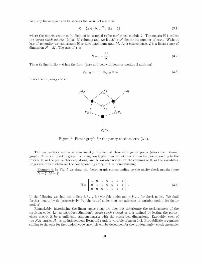
Figure 5: Factor graph for the parity-check matrix (3.4).
The parity-check matrix is conveniently represented through a factor graph (also called Tannergraph). This is a bipartite graph including two types of nodes: M function nodes (corresponding to therows of H, or the parity-check equations) and N variable nodes (for the columns of H, or the variables).Edges are drawn whenever the corresponding entry in H is non-vanishing.
Example 4: In Fig. 5 we draw the factor graph corresponding to the parity-check matrix (hereN = 7, M = 3)
H =
1 0 1 0 1 0 1
0 1 1 0 0 1 1
0 0 0 1 1 1 1
. (3.4)
In the following we shall use indices i, j, . . . for variable nodes and a, b, . . . for check nodes. We shallfurther denote by ∂i (respectively, ∂a) the set of nodes that are adjacent to variable node i (to factornode a).
Remarkably, introducing the linear space structure does not deteriorate the performances of theresulting code. Let us introduce Shannon’s parity-check ensemble: it is defined by letting the parity-check matrix H be a uniformly random matrix with the prescribed dimensions. Explicitly, each ofthe NM entries Hai is an independent Bernoulli random variable of mean 1/2. Probabilistic argumentssimilar to the ones for the random code ensemble can be developed for the random parity-check ensemble.
10

The conclusion is that random codes from this ensemble allow to communicate with arbitrarily smallblock error probability at any rate R < C(Q), where C(Q) is the capacity of the given BMS channel.
Unfortunately, linearity is not sufficient to guarantee that a code admits a low-complexity decodingalgorithm. In particular, the algorithm which we discuss in the sequel works well only for codes that canbe represented by a sparse parity-check matrix H (i.e. a parity check matrix with O(N) non-vanishingentries). Notice that a given code C has more than one representation of the form (3.1). A priori onecould hope that, given a uniformly random matrix H, a new matrix H
′ could be built such that H′ is
sparse and that its null space coincides with the one of H. This would provide a sparse representation ofC. Unfortunately, this is the case only for a vanishing fraction of matrices H, as shown by the exercisebelow.
Exercise 2: Consider a linear code C, with blocklength N , and dimension N −M (as a linearspace). Prove the following sequence of arguments.
(i) The total number of binary N ×M parity-check matrices is 2NM .
(ii) Each code C has 2(M
2 )∏Mi=1
(2i − 1
)distinct N ×M parity-check matrices H.
(iii) The number of such matrices with at most aN non-zero entries is∑aN
i=0
(NM
i
)≤ 2NMh2(a/(N−M)).
(iv) Conclude from the above that, for any given a, the fraction of parity-check matrices H thatadmit a sparse representation in terms of a matrix H
′ with at most aN ones, is of order e−Nγ
for some γ > 0.
With an abuse of language in the following we shall sometimes use the term ‘code’ to denote a paircode/parity-check matrix.
3.2 Low-Density Parity-Check Codes
Further structure can be introduced by restricting the ensemble of parity-check matrices. Low-densityparity-check (LDPC) codes are codes that have at least one sparse parity-check matrix.
Rather than considering the most general case let us limit ourselves to a particularly simple familyof LDPC ensembles, originally introduced by Robert Gallager [19]. We call them ‘regular’ ensembles.An element in this family is characterized by the blocklength N and two integer numbers k and l, withk > l. We shall therefore refer to it as the (k, l) regular ensemble). In order to construct a randomTanner graph from this ensemble, one proceeds as follows:
1. DrawN variable nodes, each attached to l half-edges andM = Nl/k (we neglect here the possibilityof Nl/k not being an integer) check nodes, each with k half edges.
2. Use an arbitrary convention to label the half edges form 1 to Nl, both on the variable node sideas well as the check node side (note that this requires that Mk = Nl).
3. Choose a permutation π uniformly at random among all permutations overNl objects, and connecthalf edges accordingly.
Notice that the above procedure may give rise to multiple edges. Typically there will be O(1) multipleedges in a graph constructed as described. These can be eliminated easily without effecting the perfor-mance substantially. From the analytical point of view, a simple choice consists in eliminating all theedges (i, a) if (i, a) occurs an even number of times, and replacing them by a single occurrence (i, a) ifit occurs an odd number of times.
Neglecting multiple occurrences (and the way to resolve them), the parity-check matrix correspondingto the graph constructed in this way does include k ones per row and l ones per column. In the sequelwe will keep l and k fixed and consider the behavior of the ensemble as N → ∞. This implies that thematrix has only O(N) non-vanishing entries. The matrix is sparse.
For practical purposes it is important to maximize the rate at which such codes enable one tocommunicate with vanishing error probability. To achieve this goal, several more complex ensembleshave been introduced. As an example, one simple idea is to consider a generic row/column weightdistribution (the weight being the number of non-zero elements), cf. Fig. 6 for an illustration. Suchensembles are usually referred to as ‘irregular’, and were introduced in [27].
11

︸ ︷︷ ︸degree 2 checks
︸ ︷︷ ︸degree 3 checks
︸ ︷︷ ︸degree dmax checks
degree 2 variables︷ ︸︸ ︷degree 3 variables︷ ︸︸ ︷ degree dmax variables︷ ︸︸ ︷
permutation π
Figure 6: Factor graph of an irregular LDPC code. Variable nodes and function nodes can have any degreebetween 2 and dmax. Half edges on the two sides are joined through a uniformly random permutation.
3.3 Weight Enumerator
As we saw in Section 2.5, the reason of the good performance of Shannon ensemble (having vanishingblock error probability at rates arbitrarily close to the capacity), can be traced back to its minimumdistance properties. This is indeed only a partial explanation (as we saw errors could be correctedwell beyond half its minimum distance). It is nevertheless instructive and useful to understand thegeometrical structure (and in particular the minimum distance properties) of typical codes from theLDPC ensembles defined above.
Let us start by noticing that, for linear codes, the distance enumerator does not depend upon thereference codeword. This is a straightforward consequence of the observation that, for any x(0) ∈ C
the set x(0) ⊕ C ≡ {x(0) ⊕ x : x ∈ C} coincides with C. We are therefore led to consider the distanceenumerator with respect to the all-zero codeword 0. This is also referred to as the weight enumerator,
N (w) = # {x ∈ C : w(x) = w } , (3.5)
where w(x) = d(x, 0) is the number of non-zero entries in x.Let us compute the expected weight enumerator N (w) ≡ EN (w). The final result is
N (w) =(lw)!(F − lw)!
F !
(N
w
)coeff[qk(z)M , zlw] . (3.6)
Here, F = Nl = Mk denotes the number of edges in the Tanner graph, qk(z) ≡ 12 [(1+z)k+(1−z)k], and,
given a polynomial p(z) and an integer n, coeff[p(z), zn] denotes the coefficient of zn in the polynomialp(z).
We shall now prove Eq. (3.6). Let x ∈ {0, 1}N be a binary word of length N and weight w. Noticethat Hx = 0 if and only if the corresponding factor graph has the following property. Consider allvariable nodes i such that xi = 1, and color in red all edges incident on these nodes. Color in blue allthe other edges. Then all the check nodes must have an even number of incident red edges. A littlethought shows that N (w) is the number of ‘colored’ factor graphs having this property, divided by thetotal number of factor graphs in the ensemble.
A valid colored graph must have wl red edges. It can be constructed as follows. First choose wvariable nodes. This can be done in
(Nw
)ways. Assign to each node in this set l red sockets, and to
each node outside the set l blue sockets. Then, for each of the M function nodes, color in red an evensubset of its sockets in such a way that the total number of red sockets is E = wl. The number of waysof doing this is8 coeff[qk(z)M , zlw]. Finally we join the variable node and check node sockets in such away that colors are matched. There are (lw)!(F − lw)! such matchings out of the total number of F !corresponding to different elements in the ensemble.
8This is a standard generating function calculation, and is explained in Appendix A.
12

0
0.1
0.2
0.3
0.4
0.5
0.6
0 0.2 0.4 0.6 0.8 1
φ(ω
)
ω
0
0.1
0.2
0.3
0.4
0.5
0.6
0 0.2 0.4 0.6 0.8 1
φ(ω
)
ω
-0.010-0.0050.0000.005
0.00 0.02 0.04-0.010-0.0050.0000.005
0.00 0.02 0.04-0.010-0.0050.0000.005
0.00 0.02 0.04
Figure 7: Logarithm of the expected weight enumerator for the (3, 6) ensemble in the large blocklengthlimit. Inset: small weight region. Notice that φ(ω) < 0 for ω < ω∗ ≈ 0.02: besides the ‘all-zero’ word thereis no codeword of weight smaller than Nω∗ in the code with high probability.
Let us compute the exponential growth rate φ(ω) of N (w). This is defined by
N (w = Nω).= eNφ(ω) . (3.7)
In order to estimate the leading exponential behavior of Eq. (3.6), we set w = Nω and estimate thecoeff[. . . , . . . ] term using the Cauchy Theorem,
coeff[qk(z)M , zwl
]=
∮qk(z)M
zlw+1
dz
2πi=
∮exp
{N [
[l
klog qk(z) − lω log z
]}dz
2πi. (3.8)
Here the integral runs over any path encircling the origin in the complex z plane. Evaluating the integralusing the saddle point method we finally get N (w)
.= eNφ, where
φ(ω) ≡ (1 − l)h(ω) +l
klog qk(z) − ωl log z , (3.9)
and z is a solution of the saddle point equation
ω =z
k
q′k(z)
qk(z). (3.10)
The typical result of such a computation is shown in Fig. 7. As can be seen, there exists ω∗ > 0 suchthat φ(ω) < 0 for ω ∈ (0, ω∗). This implies that a typical code from this ensemble will not have anycodeword of weight between 0 and N(ω∗ − ε). By linearity the minimum distance of the code is atleast ≈ Nω∗. This implies in particular that such codes can correct any error pattern over the binarysymmetric channel of weight ω∗/2 or less.
Notice that φ(ω) is an ‘annealed average’, in the terminology of disordered systems. As such, itcan be dominated by rare instances in the ensemble. On the other hand, since logNN (Nω) = Θ(N)is an ‘extensive’ quantity, we expect it to be self averaging in the language of statistical physics. Inmathematics terms one says that it should concentrate in probability. Formally, this means that thereexists a function ΦN (ω) that is non-random (i.e., does not depend upon the code) and such that
limN→∞
P {|logNN (Nω) − ΦN (ω)| ≥ Nδ} = 0 . (3.11)
13

Further we expect that ΦN (ω) = Nφq(ω) + o(N) as N → ∞. Despite being rather fundamental, boththese statements are open conjectures.
The coefficient φq(ω) is the growth rate of the weight enumerator for typical codes in the ensembles.In statistical mechanics terms, it is a ‘quenched’ free energy (or rather, entropy). By Jensen inequalityφq(ω) ≤ φ(ω). A statistical mechanics calculation reveals that the inequality is strict for general (irreg-ular) ensembles. On the other hand, for regular ensembles as the ones considered here, φq(ω) = φ(ω):the annealed calculation yields the correct exponential rate. This claim has been supported rigorouslyby the results of [47, 3, 31].
Let us finally comment on the relation between distance enumerator and the Franz-Parisi potential[18], introduced in the study of glassy systems. In this context the potential is used to probe the structureof the Boltzmann measure. One considers a system with energy function E(x), a reference configurationx0 and some notion of distance between configurations d(x, x′). The constrained partition function isthen defined as
Z(x0, w) =
∫e−E(x) δ(d(x0, x) − w) dx . (3.12)
One then defines the potential ΦN (ω) as the typical value of logZ(x0, w) when x0 is a random config-uration with the same Boltzmann distribution and w = Nω. Self averaging is expected to hold heretoo:
limN→∞
Px0 { |logZ(x0, Nω) − ΦN (ω)| ≥ Nδ } = 0 . (3.13)
Here N may denote the number of particles or the volume of the system and Px0 { · · · } indicates prob-ability with respect to x0 distributed with the Boltzmann measure for the energy function E(x0).
It is clear that the two ideas are strictly related and can be generalized to any joint distribution of Nvariables (x1, . . . , xN ). In both cases the structure of such a distribution is probed by picking a referenceconfiguration and restricting the measure to its neighborhood.
To be more specific, the weight enumerator can be seen as a special case of the Franz-Parisi potential.It is sufficient to take as Boltzmann distribution the uniform measure over codewords of a linear codeC. In other words, let the configurations be binary strings of length N , and set E(x) = 0 if x ∈ C, and= ∞ otherwise. Then the restricted partition function is just the distance enumerator with respect tothe reference codeword, which indeed does not depend on it.
4 The Decoding Problem for Sparse Graph Codes
As we have already seen, MAP decoding requires computing either marginals or the mode of the condi-tional distribution of x being the channel input given output y. In the case of LDPC codes the posteriorprobability distribution factorizes according to underlying factor graph G:
µC,y(x) =1
Z(C, y)
N∏
i=1
Q(yi|xi)
M∏
a=1
I(xi1(a) ⊕ · · · ⊕ xik(a) = 0) . (4.1)
Here (i1(a), . . . , ik(a)) denotes the set of variable indices involved in the a-th parity check (i.e., thenon-zero entries in the a-th row of the parity-check matrix H). In the language of spin models, the termsQ(yi|xi) correspond to an external random field. The factors I(xi1(a) ⊕ · · · ⊕ xik(a) = 0) can instead beregarded as hard core k-spins interactions. Under the mapping σi = (−1)xi , such interactions dependon the spins through the product σi1(a) · · ·σik(a). The model (4.1) maps therefore onto a k-spin modelwith random field.
For MAP decoding, minimum distance properties of the code play a crucial role in determining theperformances. We investigated such properties in the previous section. Unfortunately, there is no knownway of implementing MAP decoding efficiently. In this section we discuss two decoding algorithms that
14
0
0.2
0.4
0.6
0.8
1
0.016 0.020 0.024 0.028 0.032
PB
p
N=10000N=20000N=40000
0
0.01
0.02
0.03
0.04
0.05
0.016 0.020 0.024 0.028 0.032
U*
p
N=10000N=20000N=40000
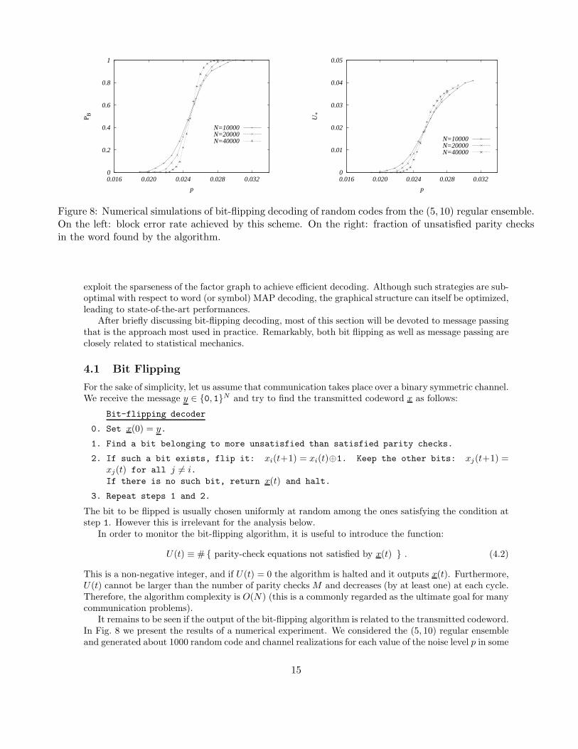
Figure 8: Numerical simulations of bit-flipping decoding of random codes from the (5, 10) regular ensemble.On the left: block error rate achieved by this scheme. On the right: fraction of unsatisfied parity checksin the word found by the algorithm.
exploit the sparseness of the factor graph to achieve efficient decoding. Although such strategies are sub-optimal with respect to word (or symbol) MAP decoding, the graphical structure can itself be optimized,leading to state-of-the-art performances.
After briefly discussing bit-flipping decoding, most of this section will be devoted to message passingthat is the approach most used in practice. Remarkably, both bit flipping as well as message passing areclosely related to statistical mechanics.
4.1 Bit Flipping
For the sake of simplicity, let us assume that communication takes place over a binary symmetric channel.We receive the message y ∈ {0, 1}N and try to find the transmitted codeword x as follows:
Bit-flipping decoder
0. Set x(0) = y.
1. Find a bit belonging to more unsatisfied than satisfied parity checks.
2. If such a bit exists, flip it: xi(t+1) = xi(t)⊕1. Keep the other bits: xj(t+1) =xj(t) for all j 6= i.If there is no such bit, return x(t) and halt.
3. Repeat steps 1 and 2.
The bit to be flipped is usually chosen uniformly at random among the ones satisfying the condition atstep 1. However this is irrelevant for the analysis below.
In order to monitor the bit-flipping algorithm, it is useful to introduce the function:
U(t) ≡ # { parity-check equations not satisfied by x(t) } . (4.2)
This is a non-negative integer, and if U(t) = 0 the algorithm is halted and it outputs x(t). Furthermore,U(t) cannot be larger than the number of parity checks M and decreases (by at least one) at each cycle.Therefore, the algorithm complexity is O(N) (this is a commonly regarded as the ultimate goal for manycommunication problems).
It remains to be seen if the output of the bit-flipping algorithm is related to the transmitted codeword.In Fig. 8 we present the results of a numerical experiment. We considered the (5, 10) regular ensembleand generated about 1000 random code and channel realizations for each value of the noise level p in some
15
U(x)
x
transmittedp < pbf
pbf < p < pc
pc < p
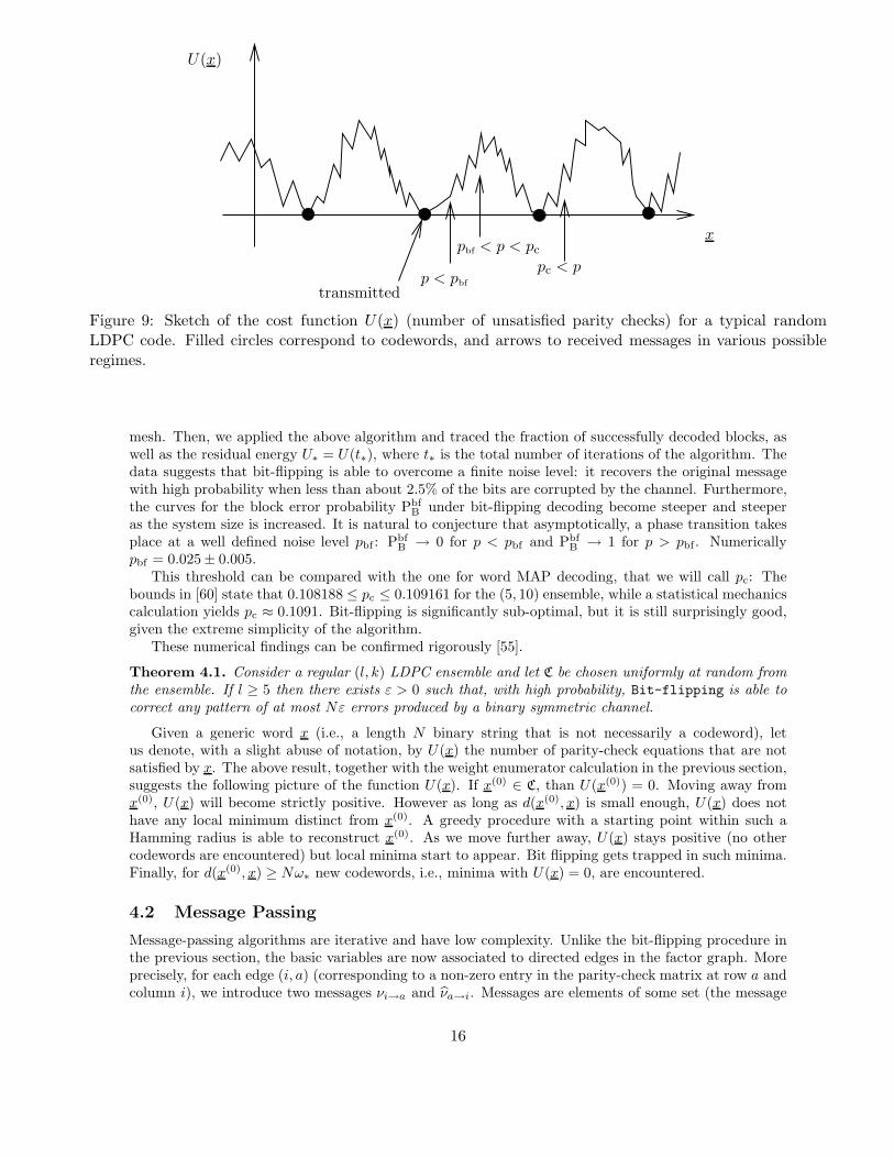
Figure 9: Sketch of the cost function U(x) (number of unsatisfied parity checks) for a typical randomLDPC code. Filled circles correspond to codewords, and arrows to received messages in various possibleregimes.
mesh. Then, we applied the above algorithm and traced the fraction of successfully decoded blocks, aswell as the residual energy U∗ = U(t∗), where t∗ is the total number of iterations of the algorithm. Thedata suggests that bit-flipping is able to overcome a finite noise level: it recovers the original messagewith high probability when less than about 2.5% of the bits are corrupted by the channel. Furthermore,the curves for the block error probability Pbf
B under bit-flipping decoding become steeper and steeperas the system size is increased. It is natural to conjecture that asymptotically, a phase transition takesplace at a well defined noise level pbf : Pbf
B → 0 for p < pbf and PbfB → 1 for p > pbf . Numerically
pbf = 0.025± 0.005.This threshold can be compared with the one for word MAP decoding, that we will call pc: The
bounds in [60] state that 0.108188 ≤ pc ≤ 0.109161 for the (5, 10) ensemble, while a statistical mechanicscalculation yields pc ≈ 0.1091. Bit-flipping is significantly sub-optimal, but it is still surprisingly good,given the extreme simplicity of the algorithm.
These numerical findings can be confirmed rigorously [55].
Theorem 4.1. Consider a regular (l, k) LDPC ensemble and let C be chosen uniformly at random fromthe ensemble. If l ≥ 5 then there exists ε > 0 such that, with high probability, Bit-flipping is able tocorrect any pattern of at most Nε errors produced by a binary symmetric channel.
Given a generic word x (i.e., a length N binary string that is not necessarily a codeword), letus denote, with a slight abuse of notation, by U(x) the number of parity-check equations that are notsatisfied by x. The above result, together with the weight enumerator calculation in the previous section,suggests the following picture of the function U(x). If x(0) ∈ C, than U(x(0)) = 0. Moving away fromx(0), U(x) will become strictly positive. However as long as d(x(0), x) is small enough, U(x) does nothave any local minimum distinct from x(0). A greedy procedure with a starting point within such aHamming radius is able to reconstruct x(0). As we move further away, U(x) stays positive (no othercodewords are encountered) but local minima start to appear. Bit flipping gets trapped in such minima.Finally, for d(x(0), x) ≥ Nω∗ new codewords, i.e., minima with U(x) = 0, are encountered.
4.2 Message Passing
Message-passing algorithms are iterative and have low complexity. Unlike the bit-flipping procedure inthe previous section, the basic variables are now associated to directed edges in the factor graph. Moreprecisely, for each edge (i, a) (corresponding to a non-zero entry in the parity-check matrix at row a andcolumn i), we introduce two messages νi→a and νa→i. Messages are elements of some set (the message
16

j a
b k
a j
Figure 10: Graphical representation of message passing updates.
alphabet) that we shall denote by M. Depending on the specific algorithm, M can have finite cardinality,or be infinite, for instance M = R. Since the algorithm is iterative, it is convenient to introduce a time
index t = 0, 1, 2, . . . and label the messages with the time at which they are updated: ν(t)i→a and ν
(t)a→i
(but we will sometimes drop the label below).The defining property of message-passing algorithms is that the message flowing from node u to v
at a given time is a function of messages entering u from nodes w distinct from v at the previous timestep. Formally, the algorithm is defined in terms of two sets of functions Φi→a( · ), Ψa→i( · ), that definethe update operations at variable and function nodes as follows
ν(t+1)i→a = Φi→a({ν(t)
b→i; b ∈ ∂i\a}; yi) , ν(t)a→i = Ψa→i({ν(t)
j→a; j ∈ ∂a\i}) . (4.3)
Notice that messages are updated in parallel and that the time counter is incremented only at variablenodes. Alternative scheduling schemes can be considered but we will stick to this for the sake ofsimplicity. After a pre-established number of iterations, the transmitted bits are estimated using allthe messages incoming at the corresponding nodes. More precisely, the estimate at function i is definedthrough a new function
x(t)i (y) = Φi({ν(t)
b→i; b ∈ ∂i}; yi) . (4.4)
A graphical representation of message passing updates is provided in Fig. 10.A specific message-passing algorithm requires the following features to be specified:
1. The message alphabet M.
2. The initialization {ν(0)i→a}, {ν
(0)i→a}.
3. The update functions {Φi→a( · )}, {Ψa→i( · )}.4. The final estimate functions {Φi( · )}.The most prominent instance of a message-passing algorithm is the Belief Propagation (BP) algo-
rithm. In this case the messages ν(t)i→a(xi) and ν
(t)a→i(xi) are distributions over the bit variables xi ∈ {0, 1}.
The message ν(t)a→i(xi) is usually interpreted as the a posteriori distributions of the bit xi given the in-
formation coming from edge a→ i. Analogously, νi→a(xi) is interpreted as the a posteriori distributionof xi, given all the information collected through edges distinct from (a, i). Since the messages normal-ization (explicitly νi→a(0) + νi→a(1) = 1) can be enforced at any time, we shall neglect overall factorsin writing down the relation between to messages (and correspondingly, we shall use the symbol ∝).
BP messages are updated according to the following rule, whose justification we will discuss in thenext section
ν(t+1)i→a (xi) ∝ Q(yi|xi)
∏
b∈∂i\a
ν(t)b→i(xi) , (4.5)
ν(t)a→i(xi) ∝
∑
{xj}
I(xi ⊕ xj1 ⊕ · · · ⊕ xjk−1= 0)
∏
j∈∂a\i
ν(t)j→a(xj) , (4.6)
17

j
b
i
a
ub→jhi→a
Figure 11: Factor graph of a regular LDPC code, and notation for the belief propagation messages.
where we used (i, j1, . . . , jk−1) to denote the neighborhood ∂a of factor node a. After any number ofiterations the single bit marginals can be estimated as follows
ν(t+1)i (xi) ∝ Q(yi|xi)
∏
b∈∂i
ν(t)b→i(xi) . (4.7)
The corresponding MAP decision for bit i (sometimes called ‘hard decision’, while νi(xi) is the ‘softdecision’) is
x(t)i = argmax
xi
ν(t)i (xi) . (4.8)
Notice that the above prescription is ill-defined when νi(0) = νi(1). It turns out that it is not reallyimportant which rule to use in this case. To preserve the 0 − 1 symmetry, we shall assume that the
decoder returns x(t)i = 0 or = 1 with equal probability.
Finally, as initial condition one usually takes ν(−1)a→i ( · ) to be the uniform distribution over {0, 1}
(explicitly ν(−1)a→i (0) = ν
(−1)a→i (1) = 1/2).
Since for BP the messages are distributions over binary valued variables, they can be described by asingle real number, that is often chosen to be the bit log-likelihood:9
hi→a =1
2log
νi→a(0)
νi→a(1), ua→i =
1
2log
νa→i(0)
νa→i(1). (4.9)
We refer to Fig. 11 for a pictorial representation of these notations. We further introduce the channellog-likelihoods
Bi =1
2log
Q(yi|0)Q(yi|1)
. (4.10)
The BP update equations (4.5), (4.6) read in this notation
h(t+1)i→a = Bi +
∑
b∈∂i\a
u(t)b→i , u
(t)a→i = atanh
{ ∏
j∈∂a\i
tanhh(t)j→a
}. (4.11)
In this language the standard message initialization would be u(−1)a→i = 0. Finally, the overall log-likelihood
at bit i is obtained by combining all the incoming messages in agreement with Eq. (4.7). One thus getsthe decision rule
x(t)i =
{0 if Bi +
∑b∈∂i u
(t)b→i > 0,
1 if Bi +∑
b∈∂i u(t)b→i < 0.
(4.12)
9The conventional definition of log-likelihoods does not include the factor 1/2. We introduce this factor here for uniformitywith the statistical mechanics convention (the h’s and u’s being analogous to effective magnetic fields).
18

Notice that we did not commit to any special decision if Bi +∑
b∈∂i u(t)b→i = 0. To keep complete
symmetry we’ll establish that the decoder returns 0 or 1 with equal probability in this case.
4.3 Correctness of Belief Propagation on Trees
The justification for the BP update equations (4.5), (4.6) lies in the observation that, whenever the
underlying factor graph is a tree, the estimated marginal ν(t)i (xi) converges after a finite number of
iterations to the correct one µi(xi). In particular, under the tree assumption, and for any t sufficiently
large, x(t)i (y) coincides with the symbol MAP decision.
In order to prove this statement, consider a tree factor graph G. Given a couple of adjacent nodesu, v, denote by G(u → v) the subtree rooted at the directed edge u → v (this contains all that can bereached from v through a non-reversing path whose first step is v → u). If i is a variable index and aa parity-check index, let µi→a( · ) be the measure over x = {xj : j ∈ G(i → a)}, that is obtained byretaining in Eq. (4.1) only those terms that are related to nodes in G(i→ a):
µi→a(x) =1
Z(i→ a)
∏
j∈G(i→a)
Q(yi|xi)∏
b∈G(i→a)
I(xi1(b) ⊕ · · · ⊕ xik(b) = 0) . (4.13)
The measure µa→i( · ) is defined analogously for the subtree G(a→ i). The marginals µi→a(xi) (respec-tively µa→i(xi)) are easily seen to satisfy the recursions
µi→a(xi) ∝ Q(yi|xi)∏
b∈∂i\a
µb→i(xi) , (4.14)
µa→i(xi) ∝∑
{xj}
I(xi ⊕ xj1 ⊕ · · · ⊕ xjk−1= 0)
∏
j∈∂a\i
µj→a(xj) , (4.15)
which coincide, apart from the time index, with the BP recursion (4.5), (4.6). That such recursionsconverges to {µi→a(xi), µa→i(xi)} follows by induction over the tree depth.
In statistical mechanics equations similar to (4.14), (4.15) are often written as recursions on theconstrained partition function. They allow to solve exactly models on trees. However they have beenoften applied as mean-field approximation to statistical models on non-tree graphs. This is often referredto as the Bethe-Peierls approximation [8].
The Bethe approximation presents several advantages with respect to ‘naive-mean field’ [61] (thatamounts to writing ‘self-consistency’ equations for expectations over single degrees of freedom). Itretains correlations among degrees of freedom that interact directly, and is exact on some non-emptygraph (trees). It is often asymptotically (in the large size limit) exact on locally tree-like graphs. Finally,it is quantitatively more accurate for non-tree like graphs and offers a much richer modeling palette.
Within the theory of disordered systems (especially, glass models on sparse random graphs), Eqs. (4.14)and (4.15) are also referred to as the cavity equations. With respect to Bethe-Peierls, the cavity ap-proach includes a hierarchy of (‘replica symmetry breaking’) refinements of such equations that aim atcapturing long range correlations [37]. This will briefly described in Section 5.
We should finally mention that several improvements over Bethe approximation have been developedwithin statistical physics. Among them, Kikuchi’s cluster variational method [24] is worth mentioningsince it motivated the development of a ‘generalized belief propagation’ algorithm, which spurred a lotof interest within the artificial intelligence community [61].
4.4 Density Evolution
Although BP converges to the exact marginals on tree graphs, this says little about its performanceson practical codes such as the LDPC ensembles introduced in Section 3. Fortunately, a rather precisepicture on the performance of LDPC ensembles can be derived in the large blocklength limit N → ∞.
19
The basic reason for this is that the corresponding random factor graph is locally tree-like with highprobability if we consider large blocklengths.
Before elaborating on this point, notice that the performance under BP decoding (e.g., the bit errorrate) is independent on the transmitted codeword. For the sake of analysis, we shall hereafter assumethat the all-zero codeword 0 has been transmitted.
Consider a factor graph G and let (i, a) be one of its edges. Consider the message ν(t)i→a sent by the
BP decoder in iteration t along edge (i, a). A considerable amount of information is contained in the
distribution of ν(t)i→a with respect to the channel realization, as well as in the analogous distribution for
ν(t)a→i. To see this, note that under the all-zero codeword assumption, the bit error rate after t iterations
is given by
P(t)b =
1
n
n∑
i=1
P
{Φi({ν(t)
b→i; b ∈ ∂i}; yi) 6= 0
}. (4.16)
Therefore, if the messages ν(t)b→i are independent, then the bit error probability is determined by the
distribution of ν(t)a→i.
Rather than considering one particular graph (code) and a specific edge, it is much simpler to take
the average over all edges and all graph realizations. We thus consider the distribution a(N)t ( · ) of ν
(t)i→a
with respect to the channel, the edges, and the graph realization. While this is still a quite difficultobject to study rigorously, it is on the other hand possible to characterize its large blocklength limit
at( · ) = limN a(N)t ( · ). This distribution satisfies a simple recursion.
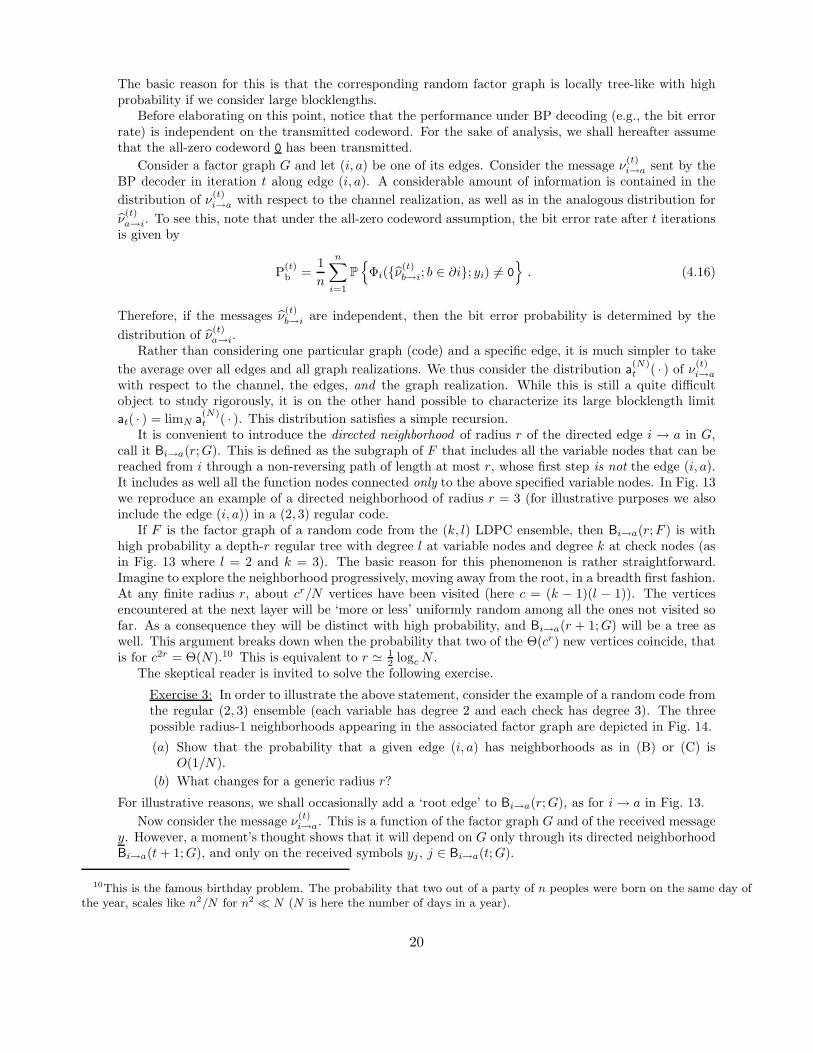
It is convenient to introduce the directed neighborhood of radius r of the directed edge i → a in G,call it Bi→a(r;G). This is defined as the subgraph of F that includes all the variable nodes that can bereached from i through a non-reversing path of length at most r, whose first step is not the edge (i, a).It includes as well all the function nodes connected only to the above specified variable nodes. In Fig. 13we reproduce an example of a directed neighborhood of radius r = 3 (for illustrative purposes we alsoinclude the edge (i, a)) in a (2, 3) regular code.
If F is the factor graph of a random code from the (k, l) LDPC ensemble, then Bi→a(r;F ) is withhigh probability a depth-r regular tree with degree l at variable nodes and degree k at check nodes (asin Fig. 13 where l = 2 and k = 3). The basic reason for this phenomenon is rather straightforward.Imagine to explore the neighborhood progressively, moving away from the root, in a breadth first fashion.At any finite radius r, about cr/N vertices have been visited (here c = (k − 1)(l − 1)). The verticesencountered at the next layer will be ‘more or less’ uniformly random among all the ones not visited sofar. As a consequence they will be distinct with high probability, and Bi→a(r + 1;G) will be a tree aswell. This argument breaks down when the probability that two of the Θ(cr) new vertices coincide, thatis for c2r = Θ(N).10 This is equivalent to r ≃ 1
2 logcN .The skeptical reader is invited to solve the following exercise.
Exercise 3: In order to illustrate the above statement, consider the example of a random code fromthe regular (2, 3) ensemble (each variable has degree 2 and each check has degree 3). The threepossible radius-1 neighborhoods appearing in the associated factor graph are depicted in Fig. 14.
(a) Show that the probability that a given edge (i, a) has neighborhoods as in (B) or (C) isO(1/N).
(b) What changes for a generic radius r?
For illustrative reasons, we shall occasionally add a ‘root edge’ to Bi→a(r;G), as for i→ a in Fig. 13.
Now consider the message ν(t)i→a. This is a function of the factor graph G and of the received message
y. However, a moment’s thought shows that it will depend on G only through its directed neighborhoodBi→a(t+ 1;G), and only on the received symbols yj , j ∈ Bi→a(t;G).
10This is the famous birthday problem. The probability that two out of a party of n peoples were born on the same day ofthe year, scales like n2/N for n2 ≪ N (N is here the number of days in a year).
20

0.05
0.10
0.15
0.20
-10 0 10 20 30 40
0.05
0.10
0.15
0.20
-10 0 10 20 30 40
0.05
0.10
0.15
0.20
-10 0 10 20 30 40
0.05
0.10
0.15
0.20
-10 0 10 20 30 40
0.05
0.10
0.15
0.20
-10 0 10 20 30 40
0.05
0.10
0.15
0.20
-10 0 10 20 30 40
0.05
0.10
0.15
0.20
-10 0 10 20 30 40
0.05
0.10
0.15
0.20
-10 0 10 20 30 40
0.05
0.10
0.15
0.20
-10 0 10 20 30 40
0.05
0.10
0.15
0.20
-10 0 10 20 30 40
Figure 12: Evolution of the probability density functions of h(t) an u(t+1) for an irregular LDPC code usedover a gaussian channel. From top to bottom t = 0, 5, 10, 50, and 140.
21

i
a
Figure 13: A radius 3 directed neighborhood Bi→a(3;G).
i
a
i
a
i
a
(A) (B) (C)
Figure 14: The three possible radius–1 directed neighborhoods in a random factor graph from the regular(2, 3) graph ensemble.
In view of the above discussion, let us consider the case in which Bi→a(t+1;G) is a (k, l)-regular tree.We further assume that the received symbols yj are i.i.d. with distribution Q(y|0), and that the updaterules (4.3) do not depend on the edge we are considering (i.e., Φi→a( · ) = Φ( · ) and Ψi→a( · ) = Ψ( · )independent of i, a).
Let ν(t) be the message passed through the root edge of such a tree after t BP iterations. Since the
actual neighborhood Bi→a(t+1;G) is with high probability a tree, ν(t)i→a
d→ ν(t) as N → ∞. The symbold→ denotes convergence in distribution. In other words, for large blocklengths, the message distributionafter t iterations is asymptotically the same that we would have obtained if the graph were a tree.
Consider now a (k, l)-regular tree, and let j → b an edge directed towards the root, at distance dfrom it. It is not hard to realize that the message passed through it after r−d−1 (or more) iterations isdistributed as ν(r−d−1). Furthermore, if j1 → b1 and j2 → b2 are both directed upwards and none belongsto the subtree rooted at the other one, then the corresponding messages are independent. Together withEq. (4.3), these observation imply that
ν(t+1) d= Φ(ν
(t)1 , . . . , ν
(t)l−1; y) , ν(t) d
= Ψ(ν(t)1 , . . . , ν
(t)k−1) . (4.17)
Here ν(t)1 , . . . , ν
(t)l−1 are i.i.d. copies of ν(t), and ν
(t)1 , . . . , ν
(t)k−1 i.i.d. copies of ν(t). Finally, y is a received
22
symbol independent from the previous variables and distributed according to Q(y|0).Equations (4.17), or the sequence of distributions that they define, are usually referred to as density
evolution. The name is motivated by the identification of the random variables with their densities(even if these do not necessarily exist). They should be parsed as follows (we are refer here to the firstequation in (4.17); an analogous phrasing holds for the second): pick l − 1 i.i.d. copies ν(t) and y with
distribution Q(y|0), compute Φ(ν(t)1 , . . . , ν
(t)l−1; y). The resulting quantity will have distribution ν(t+1).
Because of this description, they are also called ‘recursive distributional equations’.Until this point we considered a generic message passing procedure. If we specialize to BP decoding,
we can use the parametrization of messages in terms of log-likelihood ratios, cf. Eq. (4.9), and use theabove arguments to characterize the limit random variables h(t) and u(t). The update rules (4.11) thenimply
h(t+1) d= B + u
(t)1 + · · · + u
(t)l−1 , u(t) d
= atanh{tanhh
(t)1 · · · tanhh
(t)k−1
}. (4.18)
Here u(t)1 , . . . , u
(t)l−1 are i.i.d. copies of u(t), h
(t)1 , . . . , h
(t)k−1 are i.i.d. copies of h(t), and B = 1
2 log Q(y|0)Q(y|1) ,
where y is independently distributed according to Q(y|0). It is understood that the recursion is initiatedwith u(−1) = 0.
Physicists often write distributional recursions explicitly in terms of densities. For instance, the firstof the equations above reads
at+1(h) =
∫ l−1∏
b=1
dat(ub) dp(B) δ
(h−B −
l−1∑
b=1
ub
), (4.19)
where at( · ) denotes the density of u(t), and p( · ) the density of B. We refer to Fig. 12 for an illustrationof how the densities at( · ), at( · ) evolve during the decoding process.
In order to stress the importance of density evolution notice that, for any continuous function f(x),
limN→∞
E
{ 1
N
N∑
i=1
f(h(t)i→a)
}= E{f(h(t))} , (4.20)
where the expectation is taken with respect to the code ensemble. Similar expressions can be obtainedfor functions of several messages (and are particularly simple when such message are asymptotically
independent). In particular11, if we let P(N,t)b be the expected (over an LDPC ensemble) bit error rate
for the decoding rule (4.12), and let P(t)b = limN→∞ P
(N,t)b be its large blocklength limit. Then
P(t)b = P
{B + h
(t)1 + · · · + h
(t)l < 0
}+
1
2P{B + h
(t)1 + · · · + h
(t)l = 0
}, (4.21)
where h(t)1 , . . . , h
(t)l are i.i.d. copies of h(t).
4.5 The Belief Propagation Threshold
Density evolution would not be such an useful tool if it could not be simulated efficiently. The ideais to estimate numerically the distributions of the density evolution variables {h(t), u(t)}. As already
discussed this gives access to a number of statistics on BP decoding, such as the bit error rate P(t)b after
t iterations in the large blocklength limit.A possible approach consists in representing the distributions by samples of some fixed size. Within
statistical physics this is sometimes called the population dynamics algorithm (and made its first ap-pearance in the study of the localization transition on Cayley trees [46]). Although there exist more
11The suspicious reader will notice that this is not exactly a particular case of the previous statement, because f(x) = I(x <0) + 1
2I(x = 0) is not a continuous function.
23

0.00
0.05
0.10
0.15
0.20
0.00 0.05 0.10 0.15 0.20
Pb
p
0.00
0.05
0.10
0.15
0.20
0.00 0.05 0.10 0.15 0.20
Pb
p
0.00
0.05
0.10
0.15
0.20
0.00 0.05 0.10 0.15 0.20
Pb
p
0.00
0.05
0.10
0.15
0.20
0.00 0.05 0.10 0.15 0.20
Pb
p
0.00
0.05
0.10
0.15
0.20
0.00 0.05 0.10 0.15 0.20
Pb
p
0.00
0.05
0.10
0.15
0.20
0.00 0.05 0.10 0.15 0.20
Pb
p
0.00
0.05
0.10
0.15
0.20
0.00 0.05 0.10 0.15 0.20
Pb
p
0.00
0.05
0.10
0.15
0.20
0.00 0.05 0.10 0.15 0.20
Pb
p
0.0
0.3
0.6
0.0 0.1 0.20.0
0.3
0.6
0.0 0.1 0.20.0
0.3
0.6
0.0 0.1 0.20.0
0.3
0.6
0.0 0.1 0.20.0
0.3
0.6
0.0 0.1 0.20.0
0.3
0.6
0.0 0.1 0.20.0
0.3
0.6
0.0 0.1 0.20.0
0.3
0.6
0.0 0.1 0.2
0.00
0.05
0.10
0.15
0.20
0.00 0.05 0.10 0.15 0.20
Pb
p
0.00
0.05
0.10
0.15
0.20
0.00 0.05 0.10 0.15 0.20
Pb
p
0.00
0.05
0.10
0.15
0.20
0.00 0.05 0.10 0.15 0.20
Pb
p
0.00
0.05
0.10
0.15
0.20
0.00 0.05 0.10 0.15 0.20
Pb
p
0.00
0.05
0.10
0.15
0.20
0.00 0.05 0.10 0.15 0.20
Pb
p
0.00
0.05
0.10
0.15
0.20
0.00 0.05 0.10 0.15 0.20
Pb
p
0.00
0.05
0.10
0.15
0.20
0.00 0.05 0.10 0.15 0.20
Pb
p
0.00
0.05
0.10
0.15
0.20
0.00 0.05 0.10 0.15 0.20
Pb
p
0.0
0.3
0.6
0.0 0.1 0.20.0
0.3
0.6
0.0 0.1 0.20.0
0.3
0.6
0.0 0.1 0.20.0
0.3
0.6
0.0 0.1 0.20.0
0.3
0.6
0.0 0.1 0.20.0
0.3
0.6
0.0 0.1 0.20.0
0.3
0.6
0.0 0.1 0.20.0
0.3
0.6
0.0 0.1 0.2
Figure 15: The performances of two LDPC ensembles as predicted by a numerical implementation ofdensity evolution. On the left, the (3, 6) regular ensemble. On the right, an optimized irregular ensemble.Dotted curves refer (from top to bottom) to t = 0, 1, 2, 5, 10, 20, 50 iterations, and bold continuous lines
to the limit t→ ∞. In the inset we plot the expected conditional entropy EH(Xi|ν(t)i ).
efficient alternatives in the coding context (mainly based on Fourier transform, see [49, 48]), we shalldescribe population dynamics because it is easily programmed.
Let us describe the algorithm within the setting of a general message passing decoder, cf. Eq. (4.17).Given an integer N ≫ 1, one represent the messages distributions with two samples of size N : P(t) =
{ν(t)1 , . . . , ν
(t)N }, and P(t) = {ν(t)
1 , . . . , ν(t)N }. Such samples are used as proxy for the corresponding
distributions. For instance, one would approximate an expectation as
Ef(ν(t)) ≈ 1
NN∑
i=1
f(ν(t)i ) . (4.22)
The populations are updated iteratively. For instance P(t+1) is obtained from P(t) by generating
ν(t+1)1 , . . . , ν
(t+1)N independently as follows. For each i ∈ [N ], draw indices b1(i), . . . , bl(i) indepen-
dently and uniformly at random from [N ], and generate yi with distribution Q(y|0). Then compute
ν(t+1)i = Φ({ν(t)
bn(i)}; yi) and store it in P(t+1).
An equivalent description consists in saying that we proceed as if P(t) exactly represents the distri-bution of u(t) (which in this case would be discrete). If this was the case, the distribution of h(t+1) wouldbe composed of |A| · N l−1 Dirac deltas. In order not to overflow memory, the algorithm samples Nvalues from such a distribution. Empirically, estimates of the form (4.22) obtained through populationdynamics have systematic errors of order N−1 and statistical errors of order N−1/2 with respect to theexact value.
In Fig. 15 we report the results of population dynamics simulations for two different LDPC ensembles,
with respect to the BSC. We consider two performance measures: the bit error rate P(t)b and the bit
conditional entropy H(t). The latter is defined as
H(t) = limN→∞
1
N
N∑
i=1
EH(Xi|ν(t)i ) , (4.23)
and encodes the uncertainty about bit xi after t BP iterations. It is intuitively clear that, as the algorithm
24

l k R pd Shannon limit
3 4 1/4 0.1669(2) 0.21450183 5 2/5 0.1138(2) 0.14610243 6 1/2 0.0840(2) 0.11002794 6 1/3 0.1169(2) 0.1739524
Table 1: Belief propagation thresholds for a few regular LDPC ensembles.
progresses, the bit estimates improve and therefore P(t)b and H(t) should be monotonically decreasing
functions of the number of iterations. Further, they are expected to be monotonically increasing functionsof the crossover probability p. Both statement can be easily checked on the above plots, and can beproved rigorously as well.
Since P(t)b is non-negative and decreasing in t, it has a finite limit
PBPb ≡ lim
t→∞P
(t)b , (4.24)
which is itself non-decreasing in p. The limit curve PBPb is estimated in Fig. 15 by choosing t large
enough so that P(t)b is independent of t within the numerical accuracy.
Since PBPb = PBP
b (p) is a non-decreasing function of p, one can define the BP threshold
pd ≡ sup{p ∈ [0, 1/2] : PBP
b (p) = 0}. (4.25)
Analogous definitions can be provided for other channel families such as the BEC(ǫ). In general, thedefinition (4.25) can be extended to any family of BMS channels BMS(p) indexed by a real parameterp ∈ I, I ⊆ R being an interval (obviously the sup will be then taken over p ∈ I). The only conditionis that the family is ‘ordered by physical degradation’. We shall not describe this concept formally, butlimit ourselves to say that that p should be an ‘honest’ noise parameter, in the sense that the channelworsen as p increases.
Analytical upper and lower bounds can be derived for pd. In particular it can be shown that it isstrictly larger than 0 (and smaller than 1/2) for all LDPC ensembles with minimum variable degree atleast 2. Numerical simulation of density evolution allows to determine it numerically with good accuracy.In Table 4.5 we report the results of a few such results.
Let us stress that the threshold pd has an important practical meaning. For any p < pd one canachieve arbitrarily small bit error rate with high probability by just picking one random code from theensemble LDPC and using BP decoding and running it for a large enough (but independent of theblocklength) number of iterations. For p > pd the bit error rate is asymptotically lower bounded byPBP
b (p) > 0 for any fixed number of iterations. In principle it could be that after, let’s say na, a > 0iterations a lower bit error rate is achieved. However simulations show quite convincingly that this isnot the case.
In physics terms the algorithm undergoes a phase transition at pd. At first sight, such a phasetransition may look entirely dependent on the algorithm definition and not ‘universal’ in any sense. Aswe will discuss in the next section, this is not the case. The phase transition at pd is somehow intrinsic tothe underlying measure µ(x), and has a well studied counterpart in the theory of mean field disorderedspin models.
Apart from the particular channel family, the BP threshold depends on the particular code ensemble,i.e. (for the case considered here) on the code ensemble. It constitutes therefore a primary measureof the ‘goodness’ of such a pair. Given a certain design rate R, one would like to make pd as large aspossible. This has motivated the introduction of code ensembles that generalize the regular ones studiedhere (starting from ‘irregular’ ones). Optimized ensembles have been shown to allow for exceptionally
25

good performances. In the case of the erasure channel, they allowed to saturate Shannon’s fundamentallimit [27]. This is an important approach to the design of LDPC ensembles.
Let us finally mention that the BP threshold was defined in Eq. (4.25) in terms of the bit error rate.One may wonder whether a different performance parameter may yield a different threshold. As long as
such parameter can be written in the form 1N
∑i f(h
(t)i ) this is not the case. More precisely
pd = sup{p ∈ I : h(t) d→ +∞
}, (4.26)
where, for the sake of generality we assumed the noise parameter to belong to an interval I ⊆ R. Inother words, for any p < pd the distribution of BP messages becomes a delta at plus infinity.
4.6 Belief Propagation versus MAP Decoding
So far we have seen that detailed predictions can be obtained for the performance of LDPC ensemblesunder message passing decoding (at least in the large blocklength limit). In particular the thresholdnoise for reliable communication is determined in terms of a distributional recursion (density evolution).This recursion can in turn be efficiently approximated numerically, leading to accurate predictions forthe threshold.
It would be interesting to compare such predictions with the performances under optimal decodingstrategies. Throughout this section we shall focus on symbol MAP decoding, which minimizes the biterror rate, and consider a generic channel family {BMS(p)} ordered12 by the noise parameter p.
Given an LDPC ensemble, let P(N)b be the expected bit error rate when the blocklength is N . The
MAP threshold pc for such an ensemble can be defined as the largest (or, more precisely, the supremum)
value of p such that limN→∞ P(N)b = 0. In other words, for any p < pc one can communicate with
an arbitrarily small error probability, by using a random code from the ensemble, provided N is largeenough.
By the optimality of MAP decoding, pd ≤ pc. In coding theory some techniques have been developedto prove upper and lower bounds on pc [19, 52]. In particular it is easy to find ensembles for which thereexist a gap between the two thresholds (namely pd < pc strictly). Consider for instance (k, l) regularensembles with a fixed ratio l/k = 1−R. It is then possible to show that, as k, l → ∞, the BP thresholdgoes to 0 while the MAP threshold approaches the Shannon limit.
This situation is somewhat unsatisfactory. The techniques used to estimate pd and pc are completelydifferent. This is puzzling since the two thresholds can be extremely close and even coincide for someensembles. Furthermore, we know that pd ≤ pc by a general argument (optimality of MAP decoding),but this inequality is not ‘built in’ the corresponding derivations. Finally, it would be interesting to havea sharp estimate for pc.
It turns out that a sharp characterization of pc can be obtained through statistical mechanics tech-niques [42, 58, 38]. The statistical mechanics result has been proved to be a rigorous upper bound forgeneral code ensembles, and it is conjectured to be tight [39, 35].
The starting point is to consider the conditional entropy of the channel input x given the output y,HN (X |Y ). As shown in Eq. (2.16) this is given by the expectation of the log partition function appearingin Eq. (4.1) (apart from a trivial additive factor).
Let fN = EHN (X |Y )/N denote the entropy density averaged over the code ensemble. Intuitivelyspeaking, this quantity allows to estimate the typical number of inputs with non-negligible probabilityfor a given channel output. If fN is bounded away from 0 as N → ∞, the typical channel outputcorresponds to an exponential number of (approximately) equally likely inputs. If on the other handfN → 0, the correct input has to be searched among a sub-exponential number of candidates. This leadsus to identify13 the MAP threshold as the largest noise level such that fN → 0 as N → ∞.
12Such that the channel worsen as p increases. Examples are the binary symmetric or binary erasure channels.
13A rigorous justification of this identification can be obtained using Fano’s inequality.
26

The Bethe free energy provides a natural way to approximate log-partition functions on sparse graphs.It is known to be exact if the underlying graph is a tree and its stationary points are in correspondencewith the fixed points of BP. In statistical physics terms, it is the correct variational formulation for theBethe Peierls approximation. In random systems which are locally tree like, it is normally thought toprovide the correct N → ∞ limit unless long range correlations set in. These are in turn describedthrough ‘replica symmetry breaking’ (see below).
As many mean field approximations, the Bethe approximation can be thought of as a way of writingthe free energy as a function of a few correlation functions. More specifically, one considers the single-variable marginals {bi(xi) : i ∈ {1, . . . , N}}, and the joint distributions of variables involved in acommon check node {ba(xa) : a ∈ {1, . . . ,M}}. In the present case the Bethe free energy reads
FB(b) = −N∑
i=1
∑
xi
bi(xi) logQ(yi|xi) + (4.27)
+M∑
a=1
∑
xa
ba(xa) log ba(xa) −N∑
i=1
(|∂i| − 1)∑
xi
bi(xi) log2 bi(xi) .
The marginals {bi( · )}, {ba( · )} are regarded as variables. They are constrained to be probability distri-butions (hence non-negative) and to satisfy the marginalization conditions
∑
xj, j∈∂a\i
ba(xa) = bi(xi) ∀i ∈ ∂a ,∑
xi
bi(xi) = 1 ∀i . (4.28)
Further, in order to fulfill the parity-check constraints ba(xa) must be forced to vanish unless xia(1) ⊕· · · ⊕ xia(k) = 0 (as usual we use the convention 0 log 0 = 0). Since they do not necessarily coincide withthe actual marginals of µ( · ), the {ba}, {bi} are sometimes called beliefs.
Approximating the log-partition function − logZ(y) requires minimizing the Bethe free energy FB(b).The constraints can be resolved by introducing Lagrange multipliers, that are in turn expressed in termsof two families of real valued messages u ≡ {ua→i}, h = {hi→a}. If we denote by Pu(x) the distributionof a bit x whose log likelihood ratio is u (in other words Pu(0) = 1/(1+e−2u), Pu(1) = e−2u/(1+e−2u)),the resulting beliefs read
ba(xa) =1
zaIa(x)
∏
j∈∂a
Phj→a(xj) , bi(xi) =
1
ziQ(yi|xi)
∏
a∈∂i
Pua→i(xi) , (4.29)
where we introduced the shorthand Ia(x) to denote the indicator function for the a-th parity check beingsatisfied. Using the marginalization conditions (4.28) as well as the stationarity of the Bethe free energywith respect to variations in the beliefs, one obtains the fixed point BP equations
hi→a = Bi +∑
b∈∂i\a
ub→i , ua→i = atanh
∏
j∈∂a\i
tanhhj→a
. (4.30)
These in turn coincide for with the fixed point conditions for belief propagation, cf. Eqs. (4.11).The Bethe free energy can be written as a function of the messages by plugging the expressions (4.29)
into Eq. (4.27). Using the fixed point equations, we get
FB(u, h) =∑
(ia)∈E
log
[∑
xi
Pua→i(xi)Phi→a
(xi)
]− (4.31)
−N∑
i=1
log
[∑
xi
Q(yi|xi)∏
a∈∂i
Pua→i(xi)
]−
M∑
a=1
log
∑
xa
Ia(x)∏
i∈∂a
Phi→a(xi)
.
27

We are interested in the expectation of this quantity with respect to the code and channel realization,
in the N → ∞ limit. We assume that messages are asymptotically identically distributed ua→id=
u, hi→ad= h, and that messages incoming in the same node along distinct edges are asymptotically
independent. Under these hypotheses we get the limit
limN→∞
1
NEFB(u, u) = −φu,h +
∑
y
Q(y|0) log2Q(y|0) , (4.32)
where
φu,h ≡ −lEu,h log2
[∑
x
Pu(x)Ph(x)
]+ EyE{ui} log2
[∑
x
Q(y|x)Q(y, 0)
l∏
i=1
Pui(x)
]−
+l
kE{hi} log2
[∑
x1...xk
Ia(x)
k∏
i=1
Phi(xi)
]. (4.33)
Notice that the random variables u, h are constrained by Eq. (4.30), which must be fulfilled in dis-tributional sense. In other words u, h must form a fixed point of the density evolution recursion (4.18).Given this proviso, if the above assumptions are correct and the Bethe free energy is a good approxima-tion for the log partition function one expects the conditional entropy per bit to be limN→∞ fN = φu,h.This guess is supported by the following rigorous result.
Theorem 4.2. If u, h are symmetric random variables satisfying the distributional identity ud=
atanh{∏k−1
i=1 tanhhi
}, then
limN→∞
fN ≥ φu,h . (4.34)
It is natural to conjecture that the correct limit is obtained by optimizing the above lower bound,i.e.
limN→∞
fN = supu,h
φu,h , (4.35)
where, once again the sup is taken over the couples of symmetric random variables satisfying ud=
atanh{∏k−1
i=1 tanhhi
}. In fact it is easy to show that, on the fixed point, the distributional equation
hd= B +
∑l−1a=1 ua must be satisfied as well. In other words the couple u, h must be a density evolution
fixed point.This conjecture has indeed been proved in the case of communication over the binary erasure channel
for a large class of LDPC ensembles (including, for instance, regular ones).The expression (4.35) is interesting because it bridges the analysis of BP and MAP decoding. For
instance, it is immediate to show that it implies pd ≤ pc.
Exercise 4: This exercise aims at proving the last statement.
(a) Recall that u, h = +∞ constitute a density evolution fixed point for any noise level. Showthat φh,u = 0 on such a fixed point.
(b) Assume that, if any other fixed point exists, then density evolution converges to it (this canindeed be proved in great generality).
(c) Deduce that pd ≤ pc.
Evaluating the expression (4.35) implies an a priori infinite dimensional optimization problem. Inpractice good approximations can be obtained through the following procedure:
1. Initialize h, u to a couple of symmetric random variables h(0), u(0).
28

l k R pc Shannon limit
3 4 1/4 0.2101(1) 0.21450183 5 2/5 0.1384(1) 0.14610243 6 1/2 0.1010(2) 0.11002794 6 1/3 0.1726(1) 0.1739524
Table 2: MAP thresholds for a few regular LDPC ensembles and communication over the BSC(p).
2. Implement numerically the density evolution recursion (4.18) and iterate it until an approximatefixed point is attained.
3. Evaluate the functional φu,h on such a fixed point, after enforcing ud= atanh
{∏k−1i=1 tanhhi
}
exactly.
The above procedure can be repeated for several different initializations u(0), h(0). The largest of thecorresponding values of φu,h is then picked as an estimate for limN→∞ fN .
While his procedure is not guaranteed to exhaust all the possible density evolution fixed points, itallows to compute a sequence of lower bounds to the conditional entropy density. Further, one expectsa small finite number of density evolution fixed points. In particular, for regular ensembles and p > pd,a unique (stable) fixed point is expected to exist apart from the no-error one u, h = +∞. In Table 4.6we present the corresponding MAP thresholds for a few regular ensembles.
For further details on these results, and complete proofs, we refer to [39]. Here we limit ourselves toa brief discussion why the conjecture (4.35) is expected to hold from a statistical physics point of view.
The expression (4.35) corresponds to the ‘replica symmetric ansatz’ from the present problem. Thisusually breaks down if some form of long-range correlation (‘replica symmetry breaking’) arises in themeasure µ( · ). This phenomenon is however not expected to happen in the case at hand. The technicalreason is that the so-called Nishimori condition holds for µ( · ) [38]. This condition generally holds for alarge family of problems arising in communications and statistical inference. While Nishimori conditiondoes not provide an easy proof of the conjecture (4.35), it implies a series of structural properties ofµ( · ) that are commonly regarded as incompatible with replica symmetry breaking.
Replica symmetry breaking is instead necessary to describe the structure of ‘metastable states’ [17].This can be loosely described as very deep local minima in the energy landscape introduced in Section 4.1.Here ‘very deep’ means that Θ(N) bit flips are necessary to lower the energy (number of unsatisfiedparity checks) when starting from such minima. As the noise level increases, such local minima becomerelevant at the so called ‘dynamic phase transition’. It turns out that the critical noise for this phasetransition coincides with the BP threshold pd. In other words the double phase transition at pd and pc
is completely analogous to what happens in the mean field theory of structural glasses (see for instanceParisi’s lectures at this School). Furthermore, this indicates that pd has a ‘structural’ rather than purelyalgorithmic meaning.
5 Belief Propagation Beyond Coding Theory
The success of belief propagation as an iterative decoding procedure has spurred a lot of interest in itsapplication to other statistical inference tasks.
A simple formalization for this family of problems is provided by factor graphs. One is given a factorgraph G = (V, F,E) with variable nodes V , function nodes F , and edges E and considers probability
29

a b
c
d
e
x
x
x
x
x
1
2
3
5
4
Figure 16: Factor graph representation of the satisfiability formula (5.5). Circle correspond to variablesand squares to clauses. Edges are represented as dashed line if the variable is negated in the correspondingclause.
distributions that factorize accordingly
µ(x) =1
Z
∏
a∈F
ψa(x∂a) . (5.1)
Here the variables xi take values in a generic finite alphabet X , and the compatibility functions ψa :X ∂a → R+ encode dependencies among them. The prototypical problem consists in computing marginalsof the distribution µ( · ), e.g.,
µi(xi) ≡∑
x∼i
µ(x) . (5.2)
Belief propagation can be used to accomplish this task in a fast and distributed (but not necessarilyaccurate) fashion. The general update rules read
ν(t+1)i→a (xi) ∝
∏
b∈∂i\a
ν(t)b→i(xi) , ν
(t)a→i(xi) ∝
∑
{xj}
ψa(x∂a)∏
j∈∂a\i
ν(t)j→a(xj) . (5.3)
Messages are then used to estimate local marginals as follows
ν(t+1)i (xi) ∝
∏
b∈∂i
ν(t)b→i(xi) . (5.4)
The basic theoretical question is of course to establish a relation, if any between µi( · ) and νi( · ).As an example, we shall consider satisfiability [23]. Given N Boolean variables xi, i ∈ {1, . . . , N},
xi ∈ {True, False}, a formula is the logical expression obtained by taking the AND of M clauses. Eachclause is the logical OR of a subset of the variables or their negations. As an example, consider theformula (here xi denotes the negation of xi)
(x1 ∨ x2 ∨ x4)∧(x1 ∨ x2)∧(x2 ∨ x4 ∨ x5)∧(x1 ∨ x2 ∨ x5)∧(x1 ∨ x3 ∨ x5) . (5.5)
An assignment of the N variables satisfies the formula if, for each of the clause, at least one of theinvolved literals (i.e. either the variables or their negations) evaluates to True.
A satisfiability formula admits a natural factor graph representation where each clause is associatedto a factor node and each variable to a variable node. An example is shown in Fig. 16. Admitting thatthe formula has at least one satisfying assignment, it is natural to associate to a F the uniform measure
30

over such assignments µF (x). It is easy to realize that such a distribution takes the form (5.1) wherethe compatibility function ψa(x∂a) takes value 1 if the assignment x satisfies clause a and 0 otherwise.
Satisfiability, i.e., the problem of finding a solution to a satisfiability formula or proving that it isusatisfiable, is one of the prototypical NP-complete problems. Given a satisfiability formula, computingmarginals with respect to the associated distribution µF ( · ) is relevant for tasks such as counting thenumber of solutions of F or sampling them uniformly. These are well known #-P complete problems.14
The currently best algorithms for solving random instances for the K-SAT problem are based on avariant of BP, which is called survey propagation [11, 33, 11].
5.1 Proving Correctness through Correlation Decay
A simple trick to bound the error incurred by BP consists in using the correlation decay properties[1, 57] of the measure µ( · ). Let i ∈ {1, . . . , N} be a variable index and denote by xt the set of variablessitting on nodes at distance t from i. Further, denote by x≥t the set of variables whose distance from iis at least t. Then the local structure of the probability distribution (5.1)
µi(xi) =∑
x≥t
µ(xi|x≥t)µ(x≥t) =∑
xt
µ(xi|xt)µ(xt) . (5.6)
Let Bi(t) denote the subgraph induced by nodes whose distance from i is at most t, and ∂Bi(t) itsboundary (nodes whose distance from i is exactly t). Further, for any j ∈ ∂Bi(t) let a(j) be the uniquefunction nodes inside Bi(t) that is adjacent to j. It is intuitively clear that belief propagation computesthe marginal at i as if the graph did not extend beyond Bi(t). More precisely, if the initial condition
ν(0)i→a(xi) is properly normalized, then we have the exact expression
ν(t)i (xi) =
∑
xt
µ(xi|xt)∏
j∈∂Bi(t)
ν(0)j→a(j)(xj) . (5.7)
As a consequence of Eq. (5.6) and (5.7) we have
|µi(xi) − ν(t)i (xi)| ≤ sup
xt,x′
t
|µ(xi|xt) − µ(xi|x′t)| . (5.8)
This provides an upper bound on the error incurred by BP when computing the marginal of xi base onthe local structure of the underlying graph in terms of the influence of far away variables. To make thingsfully explicit, assume that the graph has girth15 g and that supxt,x′
t|µ(xi|xt)−µ(xi|x′t)| ≤ exp(−κt) for
some positive κ. This implies
|µi(xi) − ν(t)i (xi)| ≤ e−κg/2 . (5.9)
As an example of such error estimates, we shall consider random k-satisfiability [16]. This is astandard model to generate ‘synthetic’ satisfiability formulae. It amounts to picking a formula uniformlyat random among all the ones including N variables and M = Nα k-clauses (a k-clause is a clause thatinvolve exactly k distinct variables). We shall of course limit to k ≥ 2, the case k = 1 being trivial.
Consider a uniformly random variable node in the factor graph associated to a random formula, andits depth-t neighborhood Bi(t). Proceeding as in the previous section it is not hard to show that, forany fixed t, Bi(t) is with high probability (as N → ∞) a tree. An appropriate model the distributionof such a tree, is given by the tree ensemble T∗(t) described as follows. For t = 0, it is the graphcontaining a unique variable node. For any t ≥ 1, start by a single variable node (the root) and add
ld= Poisson(kα) clauses, each one including the root, and k−1 new variables (first generation variables).
14The notation #-P refers to the hardness classification for counting problems.
15Recall that the girth of a graph is the length of its shortest cycle.
31

For each one of the l clauses, the corresponding literals are non-negated or negated independently withequal probability. If t ≥ 2, generate an independent copy of T∗(t− 1) for each variable node in the firstgeneration and attach it to them.
Assume that, for a typical random tree formula T(t), the marginal distribution of the variable at theroot is weakly dependent on the values assigned at the boundary. Following the above lines, one can usethis fact to prove that BP computes good approximations for the marginals in a random k-SAT formula.In fact it turns out that an estimate of the form16
ET(t) supx
t,x′
t
|µ(xi|xt) − µ(xi|x′t)| ≤ e−κt (5.10)
can be proved if the clause density α stays below a threshold αu(k) that is estimated to behave asαu(k) = 2 log k
k [1 + ok(1)].While we refer to the original paper [40] for the details of the proof we limit ourselves to noticing
that the left hand side of Eq. (5.10) can be estimated efficiently using a density evolution procedure.This allows to estimate the threshold αu(k) numerically. Consider in fact the log-likelihood (here we areidentifying {True,False} with {+1,−1})
h(t)(xt) =1
2log
µ(+1|xt)
µ(−1|xt). (5.11)
This quantity depends on the assignment of the variables on the boundary, xt. Since we are interestedon a uniform bound over the boundary, let us consider the extreme cases
h(t)
= maxxt
h(t)(xt) , h(t) = minxt
h(t)(xt) . (5.12)
It is then possible to show that the couple (h(t), h(t)) obeys a recursive distributional equation that, as
mentioned, can be efficiently implemented numerically.
6 Belief Propagation Beyond the Binary Symmetric Channel
So far we have considered mainly the case of transmission over BMS channels, our reference examplebeing the BSC. There are many other channel models that are important and are encountered in practicalsituations. Fortunately, it is relatively straightforward to extend the previous techniques and statementsto a much larger class, and we review a few such instances in this section.
6.1 Binary Memoryless Symmetric Channels
In order to keep the notation simple, we assumed channel output to belong to a finite alphabet A. In ourmain example, the BSC, we had A = {0, 1}. But in fact all results are valid for a wider class of binarymemoryless symmetric (BMS) channels. One can prove that there is no loss of generality in assumingthe output alphabet to be the real line R (eventually completed with R = R ∪ {±∞}).
Let y = (y1, . . . , yN ) be the vector of channel outputs on input x = (x1, . . . , xN ). For a BMS the
input is binary, i.e. x ∈ {0, 1}N . Further the channel is memoryless, i.e. the probability density of
getting y ∈ RN
at output when the input is x, is
Q(y|x) =
N∏
t=1
Q(yt|xt).
16Here the sup is taken over assignments xt, x′
tthat can be extended to solutions of T(t).
32

Finally, the symmetry property can be written without loss of generality, as Q(yt|xt = 1) = Q(−yt|xt =0).
One of the most important elements in this class is the additive white Gaussian noise (AWGN)channel, defined by
yt = xt + zt , t ∈ {1, . . . , N} ,
where the sequence {zt} is i.i.d. consisting of Gaussian random variables with mean zero and varianceσ2. It is common in this setting to let xi take values in {+1,−1} instead of {0, 1} as we have assumedso far. The AWGNC transition probability density function is therefore
Q(yt|xt) =1√
2πσ2e−
(y−x)2
2σ2 .
The AWGNC is the basic model of transmission of an electrical signal over a cable (here the noise isdue to thermal noise in the receiver) and it is also a good model of a wireless channel in free space (e.g.,transmission from a satellite).
Although the class of BMS channels is already fairly large, it is important in practice to go beyondit. The extension to the non-binary case is quite straightforward and so we will not discuss it in detail.The extension to channels with memory or the asymmetric case are more interesting and so we presentthem in the subsequent two sections.
6.2 Channels With Memory
Loosely speaking, in a memoryless channel the channel acts on each transmitted bit independently. Ina channel with memory, on the other hand, the channel acts generally on the whole block of input bitstogether. An important special case of a channel with memory is if the channel can be modeled as aMarkov chain, taking on a sequence of “channel states.” Many physical channels posses this propertyand under this condition the message-passing approach can still be applied. For channels with memorythere are two problems. First, we need to determine the capacity of the channel. Second, we need todevise efficient coding schemes that achieve rates close to this capacity. It turns out that both problemscan be addressed in a fairly similar framework. Rather than discussing the general case we will look ata simple but typical example.
Let us start by computing the information rate/capacity of channels with memory, assuming thatthe channel has a Markov structure. As we discussed in Section 2.5 in the setting of BMS channels, thechannel capacity can be expressed as the difference of two entropies, namely as H(X)−H(X |Y ). Here,X denotes the binary input and Y denotes the observation at the output of the channel whose input isX . Given two random variables X , Y , this entropy difference is called the mutual information and istypically denoted by I(X ;Y ) = H(X) −H(X ;Y ).
A general channel, is defined by a channel transition probability Q(yN1 |xN
1 ) (here and below xN1
denotes the vector (x1, . . . , xN )). In order to define a joint distribution of the input and output vectors,we have to prescribe a distribution on the channel input, call it p(xN
1 ). The channel capacity is obtainedby maximizing the mutual information over all possible distributions of the input, and eventually takingthe N → ∞ limit. In formulae
C(Q) = limN→∞
supp( · )
I(XN1 ;Y N
1 )/N .
For BMS channels it is possible to show that the maximum occurs for the uniform prior: p(xN1 ) = 1/2N .
Under this distribution, I(XN1 ;Y N
1 )/N is easily seen not to depend on N and we recover the expressionin Sec. 2.5.
For channels with memory we have to maximize the mutual information over all possible distributionsover {0, 1}N (a space whose dimension is exponential in N), and take the limit N → ∞. An easier task is
33

to choose a convenient input distribution p( · ) and then compute the corresponding mutual informationin the N → ∞ limit:
I = limN→∞
I(XN1 ;Y N
1 )/N . (6.1)
Remarkably, this quantity has an important operational meaning. It is the largest rate at which we cantransmit reliably across the channel using a coding scheme such that the resulting input distributionmatches p( · ).
To be definite, assume that the channel is defined by a state sequence {σt}t≥0, taking values in afinite alphabet, such that the joint probability distribution factors in the form
p(xn1 , y
n1 , σ
n0 ) = p(σ0)
n∏
i=1
p(xi, yi, σi | σi−1). (6.2)
We will further assume that the transmitted bits (x1, ·, xN ) are iid uniform in {0, 1}. The factor graphcorresponding to (6.2) is shown in Fig. 17. It is drawn in a somewhat different way compared tothe factor graphs we have seen so far. Note that in the standard factor graph corresponding to thisfactorization all variable nodes have degree two. In such a case it is convenient not to draw the factorgraph as a bipartite graph but as a standard graph in which the nodes correspond to the factor nodesand the edges correspond to the variable nodes (which have degree two and therefore connect exactly twofactors). Such a graphical representation is also known as normal graph or as Forney-style factor graph(FSFG), in honor of Dave Forney who introduced them [15]. Let us now look at a concrete example.
σ0 σ1 σ2 σ3 σn−1 σn
x1 x2 x3 xn
p(σ0)p(x1, y1, σ1 | σ0)
p(x2, y2, σ2 | σ1)p(x3, y3, σ3 | σ2)
p(xn, yn, σn | σn−1)
Figure 17: The FSFG corresponding to (6.2).
Example 5:[Gilbert-Elliott Channel] The Gilbert-Elliot channel is a model for a fading channel,i.e., a channel where the quality of the channel is varying over time. In this model we assume thatthe channel quality is evolving according to a Markov chain. In the simplest case there are exactlytwo states, and this is the original Gilbert-Elliott channel (GEC) model. More precisely, considerthe two-state Markov chain depicted in Fig. 18. Assume that {Xt}t≥1 is i.i.d., taking values in{±1} with uniform probability.
G B
g
g
bb
Figure 18: The Gilbert-Elliott channel with two states.
The channel is either in a good state, denote it by G, or in a bad state, call it B. In either statethe channel is a BSC. Let the crossover probability in the good state be ǫG and in the bad state
34

be ǫB, with 0 ≤ ǫG < ǫB ≤ 1/2. Let P be the 2 × 2 matrix
P =
(g bg b
)
which encodes the transition probabilities between the states (the columns indicate the presentstate and the rows the next state). Define the steady state probability vector p = (pG, pB), i.e., thevector which fulfills PpT = pT . This means that in steady state the system spends a fraction pG ofthe time in state G and a fraction pB of the time in state B. If we consider e.g. the state G thenthe detailed balance condition reads pGg = pBb. From this we get p = (b/(g+ b), g/(g + b)). Moregenerally, let us assume that we have s states, s ∈ N, and that the channel in state i, i ∈ [s], isthe BSC(ǫi). Let P be the s× s matrix encoding the transition probabilities between these states.Let p denote the steady-state probability distribution vector. If (I − PT + E) is invertible then adirect check shows that p = e(I − PT + E)−1, where e is the all-one vector of length s, I is thes× s identity matrix and E is the s× s all-one matrix.
Note that the state sequence is ergodic as long as the Markov chain is irreducible (i.e. there is apath of strictly positive probability from any state to any other state) and aperiodic (i.e. therethere exists such a path for any number of steps large enough). In the original Gilbert-Elliot modelthis is true as long as 0 < g, b < 1.
Consider the computation of the maximal rate at which we can transmit reliably. We have
I(XN1 ;Y N
1 ) = H(Y N1 ) −H(Y N
1 |XN1 ).
Let us see how we can compute limN→∞H(Y N1 )/N . Because of the ergodicity assumption on the state
sequence, − 1N log p(yN
1 ) converges with probability one to limN→∞H(Y N1 )/N . It follows that if we can
compute − 1N log p(yN
1 ) for a very large sequence, then with high probability the value will be close tothe desired entropy rate. Instead of computing p(yN
1 ), let us compute p(σN , yN1 ). From this we trivially
get our desired quantity by summing,
p(yN1 ) =
∑
σN
p(σN , yN1 ).
Note that
p(σN , yN1 ) =
∑
xN ,σN−1
p(xN , σN−1, σN , yN1 )
=∑
xN ,σN−1
p(xN , σN , yN | σN−1)︸ ︷︷ ︸kernel
p(σN−1, yN−11 )
︸ ︷︷ ︸message
. (6.3)
From this we see that p(σN , yN1 ) can be computed recursively. In fact this recursion corresponds to
running the BP message-passing rules on the factor graph depicted in Fig. 17 (which is a tree): denotethe message which is passed along the edge labeled by σN by νN (σN ). Then according to the BPmessage-passing rules we have
νN (σN ) =∑
xN ,σN−1
p(xN , σN , yN | σN−1) νN−1(σN−1).
If we compare this to the recursion stated in (6.3) we see that these two recursions are identical. Inother words, νN (σN ) = p(σN , y
N1 ), so that
limN→∞
H(Y N1 )/N = − lim
N→∞log(∑
σN
νN (σN ))/N. (6.4)
35

From a practical perspective it is typically more convenient to pass normalized messages νN (σN ) so that∑σ νN (σN ) = 1. The first message ν0(σ0) = p(σ0) is already a probability distribution and, hence,
normalized, ν0(σ0) = ν0(σ0). Compute ν1(σ1) and let λ1 =∑
σ1ν1(σ1). Define ν1(σ1) = ν1(σ1)/λ1.
Now note that by definition of the message-passing rules all subsequent messages in the case of rescalingdiffer from the messages which are sent in the unscaled case only by this scale factor. Therefore, if λi
denotes the normalization constant by which we have to divide at step i so as to normalize the messagethen νN (σN ) = νN (σN )/(
∏Ni=1 λi). It follows that
limN→∞
H(Y N1 )/N = − lim
N→∞log(∑
σN
αN (σN ))/N
= − limN→∞
log(( N∏
i=1
λi
)∑
σN
αN (σN ))/N = lim
N→∞
( N∑
i=1
log(λi))/N.
It remains to compute H(Y N1 | XN
1 ). We write H(Y N1 | XN
1 )/N = H(Y N1 , XN
1 )/N − H(XN1 )/N .
The second part is trivial since the inputs are i.i.d. by assumption so that H(XN1 )/N = 1. For the
term H(Y N1 , XN
1 )/N we use the same technique as for the computation of H(Y N1 )/N . Because of
the ergodicity assumption on the state sequence, − 1N log p(yN
1 , xN1 ) converges with probability one to
limN→∞H(Y N1 , XN
1 )/N . We write p(yN1 , x
N1 ) =
∑σN
p(σN , yN1 , x
N1 ) and use the factorization
p(σN , yN1 , x
N1 ) =
∑
σN−1
p(σN−1, σN , yN1 , x
N1 )
=∑
σN−1
p(xN , σN , yN | σN−1)︸ ︷︷ ︸kernel
· p(σN−1, yN−11 , xN−1
1 )︸ ︷︷ ︸
message
.
In words, we generate a random instance XN1 and Y N
1 and run the BP algorithm on the FSFG shownin Fig. 17 assuming that both Y N
1 and XN1 are ‘quenched.’ Taking the logarithm, multiplying by minus
one and normalizing by 1/N gives us an estimate of the desired entropy.Now that we can compute the maximal rate at which we can transmit reliably, let us consider coding.
The symbol MAP decoder is
xi(y) = argmaxxip(xi | yN
1 )
= argmaxxi
∑
{xj , j 6=i}
p(xN1 , y
N1 , σ
N0 )
= argmaxxi
∑
{xj , j 6=i}
p(σ0)
N∏
j=1
p(xj , yj, σj | σj−1)IC(xN1 ).
In words, the FSFG in Fig. 17 describes also the factorization for the message-passing decoder if we addto it the factor nodes describing the definition of the code. As always, this factor graph together withthe initial messages stemming from the channel completely specify the message-passing rules, except forthe message-passing schedule. Let us agree that we alternate one round of decoding with one round ofchannel estimation. No claim as to the optimality of this scheduling rule is made.
Notice that the correlations induced by the markovian structure of the channel are in general shortranged in time. This is analogous to what happens with a one-dimensional spin model, whose correlationlength is always finite (at non-zero temperature). A good approximation to the above message passingschedule is therefore obtained by a ‘windowed’ decodes. This means that the state at time t is estimatedonly of the basis of observations between time t−R and t+R, for some finite R.
Assuming windowed decoding for channel estimation, it is not hard to show that after a fixed numberof iterations, the decoding neighborhood is again asymptotically tree-like. In the case of the GEC thechannel symmetry can be used to reduce to the all-zero codeword. Therefore, we can employ thetechnique of density evolution to determine thresholds and to optimize the ensembles.
36

0.1
0.2
0.3
-10 0 10 20 30 40 50 60 70
1
2
-5 -4 -3 -2 -1 0 1 2 3 4 5
0.1
0.2
0.3
-10 0 10 20 30 40 50 60 70
1
2
-5 -4 -3 -2 -1 0 1 2 3 4 5
0.1
0.2
0.3
-10 0 10 20 30 40 50 60 70
1
2
-5 -4 -3 -2 -1 0 1 2 3 4 5
0.1
0.2
0.3
-10 0 10 20 30 40 50 60 70
1
2
-5 -4 -3 -2 -1 0 1 2 3 4 5
Figure 19: Density evolution for the GEC at iteration 1, 2, 4, and 10. The left pictures show the densitiesof the messages which are passed from the code towards the part of the FSFG which estimates the channelstate. The right hand side shows the density of the messages which are the estimates of the channel stateand which are passed to the FSFG corresponding to the code.
Example 6:[GEC: State Estimation] For the case of transmission over the GEC the iterativedecoder implicitly also estimates the state of the channel. Let us demonstrate this by means ofthe following example. We pick a GEC with three states. Let
P =
0.99 0.005 0.020.005 0.99 0.020.005 0.005 0.96
,
which has a steady state probability vector of p ≈ (0.4444, 0.4444, 0.1112). Finally, let the channelparameters of the BSC in these three states be (ǫ1, ǫ2, ǫ3) ≈ (0.01, 0.11, 0.5). This corresponds to
an average error probability of ǫavg =∑3
i=1 piǫi ≈ 0.108889. Using the methods described above,the capacity of this channel (assuming uniform inputs) can be computed to be equal to C ≈ 0.583bits per channel use. This is markedly higher than 1 − h(ǫavg) ≈ 0.503444, which is the capacityof the BSC(ǫavg). The last channel is the channel which we experience if we ignore the Markovstructure.
Fig. 19 shows the evolution of the densities for an optimized ensemble of rate r ≈ 0.5498. Thepictures on the right correspond to the messages which are passed from the part of the factor
37

graph which estimates the state towards the part of the factor graph which describes the code.These messages therefore can be interpreted as the current estimate of the state the channel isin at a given point in time. Note that after 10 iterations 5 clear peaks emerge. These peaks areat ± log(0.99/0.01) ≈ ±4.595, ± log(0.9/0.1) ≈ ±2.197, ± log(0.5/0.5) = 0. They correspond tothe received likelihoods in the three possible channel states. In other words, the emergence of thepeaks shows that at this stage the system has identified the channel states with high reliability.This is quite pleasing. Although the channel state is not known to the receiver and can not beobserved directly, in the region where the iterative decoder works reliably it also automaticallyestimates the channel state with high confidence.
Although we only looked a very particular example it is quite typical of the general situation: aslong as the channel memory can be described by a Markov chain the factor graph approach applies andwe can use message-passing schemes to construct efficient coding schemes [14, 4, 21, 22, 25, 43].
6.3 Asymmetric Channels - The Z Channel
Let us now consider the second generalization, namely the case of non-symmetric channels.Consider the channel depicted on the right of Fig. 1. For obvious reasons it is called the Z channel
(ZC). This channel has binary input and it is memoryless but it is not symmetric. Nevertheless, essen-tially the same type of analysis which we performed in Section 4 can be applied to this case as well.Symmetry is therefore a nice property to have but it is not essential.
Consider the capacity of this channel. Since the channel is not symmetric the capacity is not neces-sarily given by the mutual information between channel input and channel output for a uniform inputdistribution of the input. We must instead maximize the mutual information over the input distribu-tion. Since the channel is memoryless, it can be assumed that the input is given by a sequence of i.i.d.bernoulli variables. Assuming that p(xi = 0) = α, the output distribution is
(p(yi = 0), p(yi = 1)) = (αp, 1 − αp),
so that the mutual information Iα(X ;Y ) for a fixed α is equal to
Iα(X ;Y ) = H(Y ) −H(Y | X) = h(αp) − αh(p). (6.5)
Some calculus reveals that the optimal choice of α is
α(p) =pp/p
1 + ppp/p, (6.6)
so thatCZC(p) = h(α(p)p) − α(p)h(p).
Fig. 20 compares CZC(p) with Iα= 12(X ;Y ), i.e., it compares the capacity with the transmission rate
which is achievable with uniform input distribution. This is important and surprising – only little islost by insisting on an uniform input distribution: the rate which is achievable by using a uniform inputdistribution is at least a fraction 1
2e ln(2) ≈ 0.924 of capacity over the entire range of p (with equalitywhen p approaches one). Even more fortunate, from this perspective the Z channel is the extremal case[32, 54]: the information rate of any binary-input memoryless channel when the input distribution isthe uniform one is at least a fraction 1
2e ln(2) of its capacity. From the above discussion we concludethat, when dealing with asymmetric channels, not much is lost if we use a binary linear coding scheme(inducing a uniform input distribution).
Consider the density evolution analysis. Because of the lack of symmetry we can no longer makethe all-one codeword assumption. Therefore, it seems at first that we have to analyze the behavior ofthe decoder with respect to each codeword. Fortunately this is not necessary. First note that, since weconsider an ensemble average, only the type of the codeword matters. More precisely, let us say that acodeword has type τ if the fraction of zeros is τ . For x ∈ C, let τ(x) be its type. Let us assume that we
38

0.0 ǫ
Figure 20: Comparison of CZC(p) (solid curve) with Iα= 12(X;Y ) (dashed curve), both measured in bits.
use an LDPC ensemble whose dominant type is one-half. This means that “most” codewords containroughly as many zeros as one. Although it is possible to construct degree-distributions which violatethis constraint, “most” degree distributions do fulfill it. Under this assumption there exists some strictlypositive constant γ such that
P{τ(x) 6∈ [1/2 − δ/
√n, 1/2 + δ/
√n]}≤ e−δ2γ , (6.7)
where the probability is with respect to a uniformly random codeword x. We can therefore analyze theperformance of such a system in the following way: determine the error probability assuming that thetype of the transmitted codeword is “close” to the typical one. Since sublinear changes in the type donot figure in the density analysis, this task can be accomplished by a straightforward density evolutionanalysis. Now add to this the probability that the type of a random codeword deviates significantlyfrom the typical one. The second term can be made arbitrarily small (see right hand side of (6.7)) bychoosing δ sufficiently large.
We summarize: if we encounter a non-symmetric channel and we are willing to sacrifice a smallfraction of capacity then we can still use standard LDPC ensembles (which impose a uniform inputdistribution) to transmit at low complexity. If it is crucial that we approach capacity even closer, a moresophisticated approach is required. We can combine LDPC ensembles with non-linear mappers whichmap the uniform input distribution imposed by linear codes into a non-uniform input distribution atthe channel input in order to bring the mutual information closer to capacity. For a detailed discussionon coding for the Z-channel we refer the reader to [34, 59, 5].
7 Open Problems
Let us close by reviewing some of the most important open challenges in the channel coding problem.
7.1 Order of Limits
Density evolution computes the limit
limt→∞
limN→∞
E[P(N,t)b ].
In words we determined the limiting performance of an ensemble under a fixed number of iterations asthe blocklength tends to infinity and then let the number of iterations tend to infinity. As we have seen,this limit is relatively easy to compute. What happens if the order of limits is exchanged, i.e., how doesthe limit
limN→∞
limt→∞
E[P(N,t)b ]
39

behave? This limit is closer in spirit to the typical operation in practice: for each fixed length the BPdecoder continues until no further progress is achieved. We are interested in the limiting performanceas the blocklength tends to infinity.
For the BEC it is known that the two limits coincide. If we combine this with the fact that for theBEC the performance is a monotone function in the number of iterations (any further iteration can onlymake the result better) then we get the important observation that regardless of how we take the limit(jointly or sequentially), as long as both the blocklength as well as the number of iterations tend toinfinity we get the same result. From a practical perspective this is comforting to know: it shows thatwe can expect a certain robustness of the performance with respect to the details of the operation.
It is conjectured that the same statement holds for general BMS channels. Unfortunately, no proofis known.
7.2 Finite-Length Performance
The threshold gives an indication of the asymptotic performance: for channel parameters which arebetter than the threshold sufficiently long codes allow transmission at an arbitrarily low probability ofbit error. If, on the other hand, we transmit over a channel which has a parameter that is worse than thethreshold then we can not hope to achieve a low probability of error. This is an important insight butfrom a practical perspective we would like to know how fast the finite-length performance approaches thisasymptotic limit. There can be many different ensembles that all have the same asymptotic performancebut that might have a substantially different finite-length behavior. Can we predict which one we shouldchoose a priori without having to resort to simulations? The typical convergence of the performance tothe asymptotic limit is shown in Fig. 21. The points correspond to simulation results whereas the solidcurves correspond to a general scaling conjecture [2]. Roughly speaking, this scaling conjecture statesthat around the threshold the error probability behaves as follows: Let the channel be parameterizedby ǫ with increasing ǫ indicating a worsening of the channel. Let ǫd be the BP threshold, and definez =
√n(ǫ− ǫd). Then for z fixed and n tending to infinity we have
PB(n, ǫ) = Φ (z/α)(1 + o(1)
),
where Φ( · ) is the error function (i.e. Φ(x) is the probability that a standard normal random variable issmaller than x), and α is a constant which depends on the channel as well as on the channel.
For the BEC this scaling law has been shown to be correct [2]. In fact, even a refined version is
known [13]: define z =√n(ǫ− ǫd + βn− 2
3 ) where β is a constant depending on the ensemble. Then forz fixed and n tending to infinity we have
PB(n, ǫ) = Q (z/α)(1 +O
(n−1/3
)).
For general channels on the other hand the problem is largely open. If proved to be correct, finitelength scaling laws could be used as a tool for an efficient finite-length optimization.
7.3 Capacity-Achieving Codes
For the most part we have taken the point of view that we are given an ensemble of codes and a familyof channels and we would like to determine the performance of this combination. For instance, themost fundamental question is to determine the threshold noise for such a code/decoder combination.Hopefully this threshold is close to the best possible as determined by Shannon’s capacity formula.
But we can take a more active point of view. Given a family of channels how should we choose theensemble in order for the threshold noise to be as high as possible. In other words, can we approach thecapacity of the channel?
For the BSC this question has been answered by Luby, Mitzenmacher, Shokrollahi, Spielman, andSteman in [27]. These authors showed that by a suitable choice of the degree distribution one can
40

0.06 0.065 0.07 0.075 0.08 0.085
10-4
10-3
10-2
10-1
ǫ
PB
ǫd
Figure 21: Performance of the BP decoder for the (3, 6)-regular ensemble when transmission takes placeover the BSC. The block lengths are n = 2i, i = 10, · · · , 20. The dots correspond to simulations. For mostsimulation points the 95% confidence intervals are smaller than the dot size. The lines correspond to theanalytic approximation based on scaling laws.
approach the capacity arbitrarily closely. More precisely, in order to approach capacity up to a fractionδ the average degree has to grow like log(1/δ) and this is the best possible. For general channels it isnot known whether capacity can be achieved. Although the resolution of this problem will most likelyonly have a small practical implication it is without doubt the most important open theoretical problemin this area.
A A Generating Function Calculation
We want to compute the number of ways of picking n distinct objects from M groups each containingk objects, in such a way that the number of selected elements in each group is even. Let us denote thisnumber by Cn. The result of this computation is used in Section 3.3, where we claimed the result to beCn = coeff[qk(z)M , zn] (in that case n = lw).
First notice that given m1, . . . ,mM all even, the number of ways of choosing m1 objects from thefirst group, m2 from the second, etc is
(k
m1
)(k
m2
)· · ·(
k
mM
). (A.1)
The desired number Cn is the sum of this quantity over the even numbers m1, · · · ,mn such thatm1, . . . ,mM ∈ {0, . . . k} and m1 + · · · +mM = n. The corresponding generating function is
C(z) ≡kM∑
n=0
Cnzn =
even∑
m1...mn
(k
m1
)(k
m2
)· · ·(
k
mM
)zm1 · · · zmN , (A.2)
the sum being restricted over even integers m1, . . . ,mM ∈ {0, . . . k}. We now notice that the sumfactorizes yielding
C(z) =
{∑
meven
(k
m
)zm
}M
= qk(z)M , (A.3)
which proves the claim.
41

Acknowledgments
We would like to thank Jean-Philippe Bouchaud and Marc Mezard for organizing the 2006 SummerSchool on Complex Systems in Les Houches. We would also like to thank Cyril Measson and ChristineNeuberg with their help in creating Fig. 19.
References
[1] D. Aldous and J. M. Steele, The Objective Method: Probabilistic Combinatorial Optimizationand Local Weak Convergence, in Probability on discrete structures, H. Kesten, ed., Springer, NewYork, 2004.
[2] A. Amraoui, A. Montanari, T. Richardson, and R. Urbanke, Finite-length scaling foriteratively decoded LDPC ensembles, in Proc. 41th Annual Allerton Conference on Communication,Control and Computing, Monticello, IL, 2003.
[3] O. Barak and D. Burshtein, Lower bounds on the spectrum and error rate of LDPC codeensembles, in Proc. of the IEEE Int. Symposium on Inform. Theory, Adelaide, Australia, September4–9 2005, pp. 42–46.
[4] G. Bauch, H. Khorram, and J. Hagenauer, Iterative equalization and decoding in mobilecommunications systems, in Proceedings of GLOBECOM, 1997.
[5] A. Bennatan and D. Burshtein, Iterative decoding of LDPC codes over arbitrary discrete-memoryless channels, in Proceedings of the 41-st Allerton Conference on Communication, Control,and Computing, Monticello, IL, Oct. 2003, pp. 1416–1425.
[6] E. R. Berlekamp, Algebraic Coding Theory, Aegean Park Press, 1984.
[7] C. Berrou, A. Glavieux, and P. Thitimajshima, Near Shannon limit error-correcting codingand decoding, in Proceedings of ICC’93, Geneve, Switzerland, May 1993, pp. 1064–1070.
[8] H. A. Bethe, Statistical theory of superlattices, Proc. Roy. Soc. London A, 150 (1935), pp. 552–558.
[9] R. E. Blahut, Theory and Practice of Error Control Codes, Addison-Wesley, 1983.
[10] L. E. Boltzmann, Vorlesungen uber Gastheorie, J.A. Barth, Leipzig, 1896.
[11] A. Braunstein, M. Mezard, and R. Zecchina, Survey propagation: algorithm for satisfiability.arXiv:cond-math/cond-mat/0212002.
[12] T. M. Cover and J. A. Thomas, Elements of Information Theory, Wiley, New York, 1991.
[13] A. Dembo and A. Montanari, Finite size scaling for the core of large random hypergraphs.Xarch:math.PR/0702007, 2007.
[14] C. Douillard, A. Picart, M. Jezequel, P. Didier, C. Berrou, and A. Glavieux, Iterativecorrection of intersymbol interference: Turbo-equalization, European Trans. on Commun., 6 (1995),pp. 507–511.
[15] G. D. Forney, Jr., Codes on graphs: Normal realizations, IEEE Trans. Inform. Theory, 47 (2001),pp. 520–548.
[16] J. Franco and M. Paull, Probabilistic analysis of the Davis-Putnam procedure for solving sat-isfiability, Discrete Appl. Math, 5 (1983), pp. 77–87.
[17] S. Franz, M. Leone, A. Montanari, and F. Ricci-Tersenghi, Dynamic phase transition fordecoding algorithms, Phys. Rev. E, 22 (2002), p. 046120.
[18] S. Franz and G. Parisi, Recipes for metastable states in spin glasses, J. Physique I, 5 (1995),p. 1401.
[19] R. G. Gallager, Low-density parity-check codes, IRE Transactions on Information Theory, 8(1962), pp. 21–28.
42

[20] , Information theory and reliable communication, Wiley, 1968.
[21] J. Garcia-Frias and J. D. Villasenor, Combining hidden Markov source models and parallelconcatenated codes, IEEE Communications Letters, 1 (1997), pp. 111–113.
[22] , Turbo decoders for Markov channels, IEEE Commun. Lett., 2 (1998), pp. 257–259.
[23] M. R. Garey and D. S. Johnson, Computers and Intractability: A Guide to the Theory ofNP-Completeness, W. H. Freeman & Co., New York, 1979.
[24] R. Kikuchi, A theory of cooperative phenomena, Phys. Rev., 81 (1951), pp. 988–1003.
[25] F. R. Kschischang and A. W. Eckford, Low-density parity-check codes for the gilbert-elliotchannel, in Proc. 41th Annual Allerton Conference on Communication, Control and Computing,Monticello, IL, 2003.
[26] S. Lin and D. J. Costello, Jr., Error Control Coding, Prentice-Hall, 2nd ed., 2004.
[27] M. Luby, M. Mitzenmacher, A. Shokrollahi, D. A. Spielman, and V. Stemann, Practicalloss-resilient codes, in Proceedings of the 29th annual ACM Symposium on Theory of Computing,1997, pp. 150–159.
[28] D. J. C. MacKay, Good error correcting codes based on very sparse matrices, IEEE Trans. Inform.Theory, 45 (1999), pp. 399–431.
[29] D. J. C. MacKay, Information Theory, Inference & Learning Algorithms, Cambridge UniversityPress, Cambridge, 2002.
[30] D. J. C. MacKay and R. M. Neal, Good codes based on very sparse matrices, in Cryptographyand Coding. 5th IMA Conference, C. Boyd, ed., no. 1025 in Lecture Notes in Computer Science,Springer, Berlin, 1995, pp. 100–111.
[31] N. Macris, Correlation inequalities: a useful tool in the theory of LDPC codes, in Proc. of theIEEE Int. Symposium on Inform. Theory, Adelaide, Australia, Sept. 2005, pp. 2369 – 2373.
[32] E. E. Majani and H. Rumsey, Jr., Two results on binary-input discrete memoryless channels,in Proc. of the IEEE Int. Symposium on Inform. Theory, June 1991, p. 104.
[33] E. Maneva, E. Mossel, and M. J. Wainwright, A new look at survey propagation and itsgeneralizations, in SODA, Vancouver, Canada, 2005.
[34] R. J. McEliece, Are turbo-like codes effective on nonstandard channels?, IEEE inform. TheorySoc. Newslett., 51 (2001), pp. 1–8.
[35] C. Measson, A. Montanari, T. Richardson, and R. Urbanke, The Generalized Area The-orem and Some of its Consequences. submitted to IEEE IT, 2005.
[36] M. Mezard and A. Montanari, Information, Physics and Computation, Clarendon Press -Oxford, 2007. to be published.
[37] M. Mezard and G. Parisi, The bethe lattice spin glass revisited, Eur. Phys. J. B, 20 (2001),p. 217.
[38] A. Montanari, The glassy phase of Gallager codes, Eur. Phys. J. B, 23 (2001), pp. 121–136.
[39] , Tight bounds for LDPC and LDGM codes under MAP decoding, IEEE Trans. Inform. Theory,51 (2005), pp. 3221–3246.
[40] A. Montanari and D. Shah, Counting good truth assignments of random k-sat formulae, inSODA, New Orleans, USA, Jan. 2007, pp. 1255–1264.
[41] R. Motwani and P. Raghavan, Randomized Algorithms, Cambridge University Press, Cam-bridge, 1995.
[42] T. Murayama, Y. Kabashima, D. Saad, and R. Vicente, Statistical physics of regular low-density parity-check error-correcting codes, Phys. Rev. E, 62 (2000), p. 1577.
[43] C. Neuberg, Gilbert-Elliott channel and iterative decoding. EPFL, Semester Project (Supervisor:Cyril Meason), 2004.
43

[44] H. Nishimori, Statistical Physics of Spin Glasses and Information Processing, Oxford UniversityPress, Oxford, 2001.
[45] J. Pearl, Fusion, propagation, and structuring in belief networks, Artificial Intelligence, 29 (1998),pp. 241–288.
[46] P. W. A. R. Abou-Chacra and D. J. Thouless, A selfconsistent theory of localization, J. PhysC, 6 (1973), p. 1734.
[47] V. Rathi, On the asymptotic weight and stopping set distribution of regular LDPC ensembles,IEEE Trans. Inform. Theory, 52 (2006), pp. 4212–4218.
[48] T. Richardson and H. Jin, A new fast density evolution, in Proc. of the IEEE Inform. TheoryWorkshop, Monte Video, Uruguay, Feb. 2006. pp. 183–187.
[49] T. Richardson and R. Urbanke, The capacity of low-density parity check codes under message-passing decoding, IEEE Trans. Inform. Theory, 47 (2001), pp. 599–618.
[50] , Modern Coding Theory, Cambridge University Press, 2007. to be published.
[51] P. Rujan, Finite temperature error-correcting codes, Phys. Rev. Lett., 70 (1993), pp. 2968–2971.
[52] I. Sason and S. Shamai, Performance Analysis of Linear Codes under Maximum-LikelihoodDecoding: A Tutorial, vol. 3 of Foundations and Trends in Communications and Information Theory,NOW, Delft, the Netherlands, July 2006.
[53] C. E. Shannon, A mathematical theory of communication, Bell System Tech. J., 27 (1948), pp. 379–423, 623–656.
[54] N. Shulman and M. Feder, The uniform distribution as a universal prior, IEEE Trans. Inform.Theory, 50 (2004), pp. 1356–1362.
[55] M. Sipser and D. A. Spielman, Expander codes, IEEE Trans. Inform. Theory, 42 (1996),pp. 1710–1722.
[56] N. Sourlas, Spin-glass models as error-correcting codes, Nature, 339 (1989), pp. 693–695.
[57] S. Tatikonda and M. Jordan, Loopy belief propagation and Gibbs measures, in Proc. Uncertaintyin Artificial Intell., Alberta, Canada, Aug. 2002, pp. 493–500.
[58] J. van Mourik, D. Saad, and Y. Kabashima, Critical noise levels for LDPC decoding, PhysicalReview E, 66 (2002).
[59] C.-C. Wang, S. R. Kulkarni, and H. V. Poor, Density evolution for asymmetric memorylesschannels, IEEE Trans. Inform. Theory, 51 (2005), pp. 4216–4236.
[60] G. Wiechman and I. Sason, On the parity-check density and achievable rates of LDPC codes formemoryless binary-input output-symmetric channels, in Proc. of the Allerton Conf. on Commun.,Control and Computing, Monticello, IL, USA, September 28–30 2005, pp. 1747–1758.
[61] J. S. Yedidia, W. T. Freeman, and Y. Weiss, Constructing free energy approximations andgeneralized belief propagation algorithms, IEEE Trans. Info.Theory, 51 (2005), pp. 2282–2313.
44