Embed Size (px)
Citation preview
Modern Control SystemEKT 308
• General Introduction • Introduction to Control System• Brief Review - Differential Equation - Laplace Transform
Course Assessment
• Lecture 3 hours per week Number of units 3
• Final Examination 50 marks• Class Test 1 10 marks• Class Test 2 10 marks• Mini Project 15 marks• Assignment/Quiz 15 marks
Course Outcomes
• CO1: : The ability to obtain the mathematical model for electrical and mechanical systems and solve state equations.
• CO2: : The ability to perform time domain analysis with response to test inputs and to determine the stability of the system.
• CO3: The ability to perform frequency domain analysis of linear system and to evaluate its stability using frequency domain methods.
• CO4: The ability to design lag, lead , lead-lag compensators for linear control systems.
Text Book References
• Dorf, Richard C., Bishop, Robert H., “Modern Control Systems”, Pearson, Twelfth Edition, 2011
• Nise , Norman S. , “Control Systems Engineering”, John Wiley and Sons , Fourth Edition, 2004.
• Kuo B.C., "Automatic Control Systems", Prentice Hall, 8th Edition, 1995
• Ogata, K, "Modern Control Engineering"Prentice Hall, 1999
• Stanley M. Shinners, “Advanced Modern Control System Theory and Design”, John Wiley and Sons, 2nd Edition. 1998
What is a Control System ?
• A device or a set of devices• Manages, commands, directs or
regulates the behavior of other devices or systems.
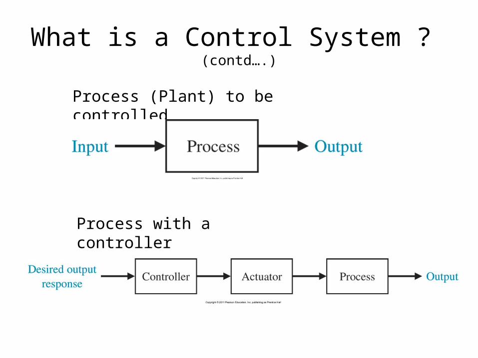
What is a Control System ? (contd….)
Process (Plant) to be controlled
Process with a controller
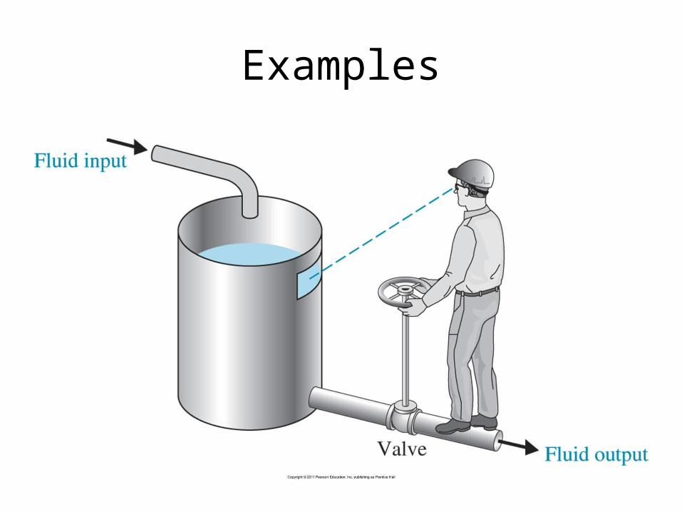
Examples
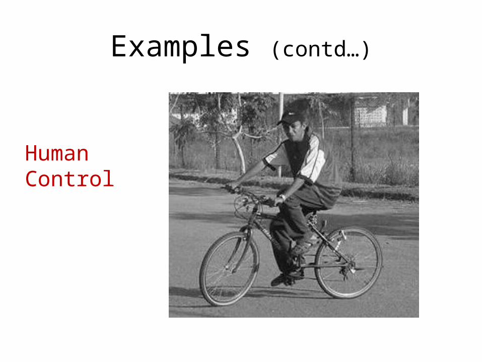
Examples (contd…)
Human Control
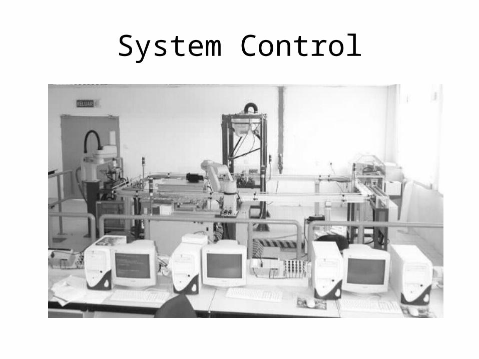
System Control
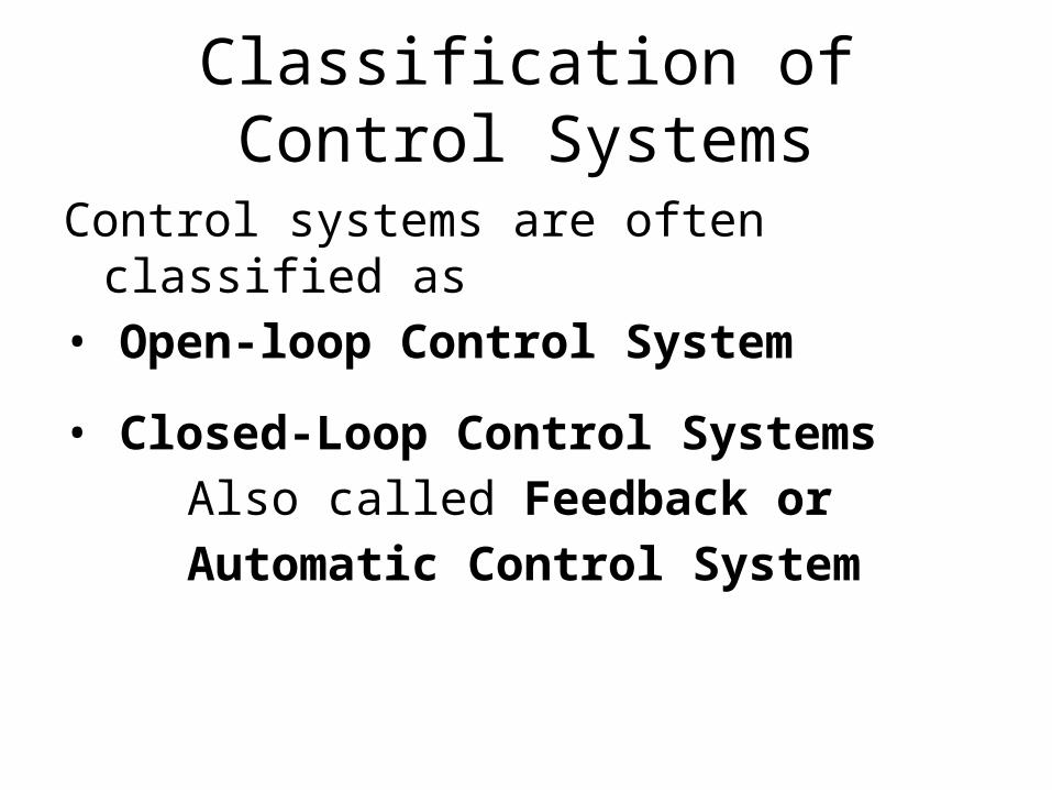
Classification of Control Systems
Control systems are often classified as• Open-loop Control System
• Closed-Loop Control Systems Also called Feedback or Automatic Control System
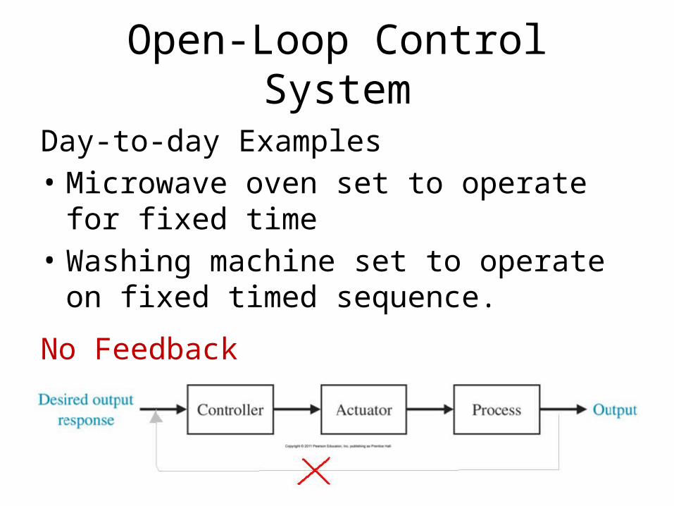
Open-Loop Control System
Day-to-day Examples• Microwave oven set to operate for fixed time• Washing machine set to operate on fixed
timed sequence.
No Feedback
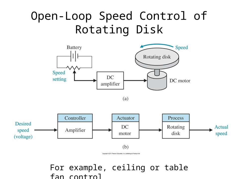
Open-Loop Speed Control of Rotating Disk
For example, ceiling or table fan control
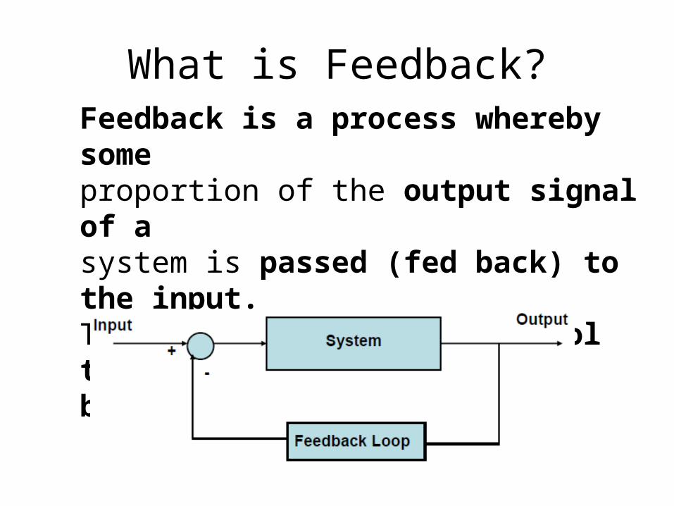
What is Feedback?Feedback is a process whereby someproportion of the output signal of asystem is passed (fed back) to the input.This is often used to control the dynamicbehavior of the System
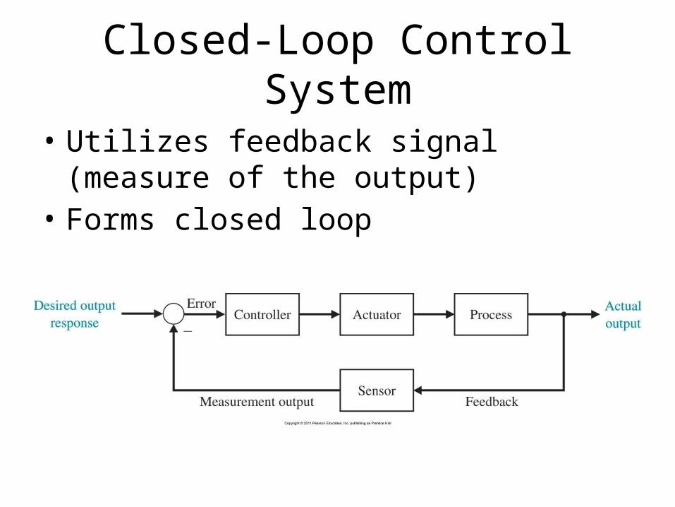
Closed-Loop Control System
• Utilizes feedback signal (measure of the output)
• Forms closed loop
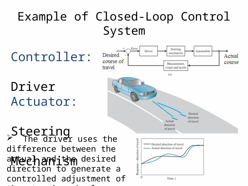
Example of Closed-Loop Control System
Controller: DriverActuator: Steering Mechanism
The driver uses the difference between the actual and the desired direction to generate a controlled adjustment of the steering wheel
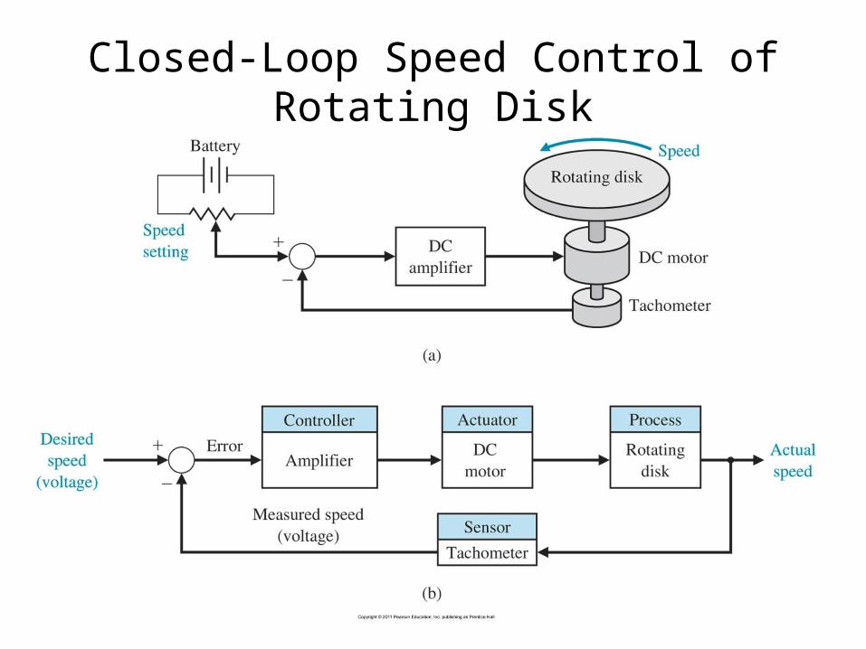
Closed-Loop Speed Control of Rotating Disk
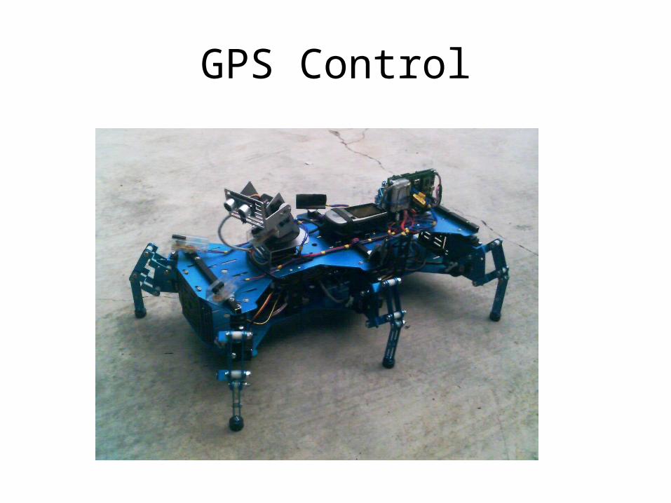
GPS Control
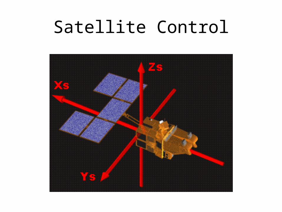
Satellite Control
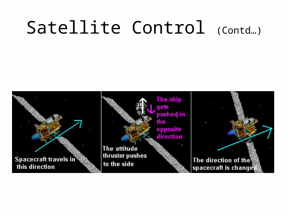
Satellite Control (Contd…)
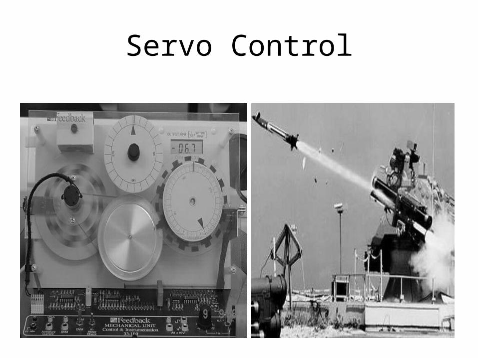
Servo Control
Introduction to Scilab
• Scilab • Xcos
Differential Equation
0..... 011
1
1
adx
dya
dx
yda
dx
yda
n
n
nn
n
n
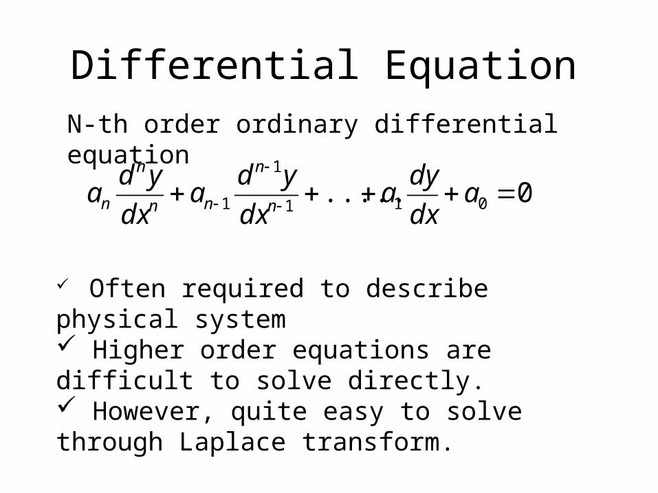
N-th order ordinary differential equation
Often required to describe physical system Higher order equations are difficult to solve directly. However, quite easy to solve through Laplace transform.
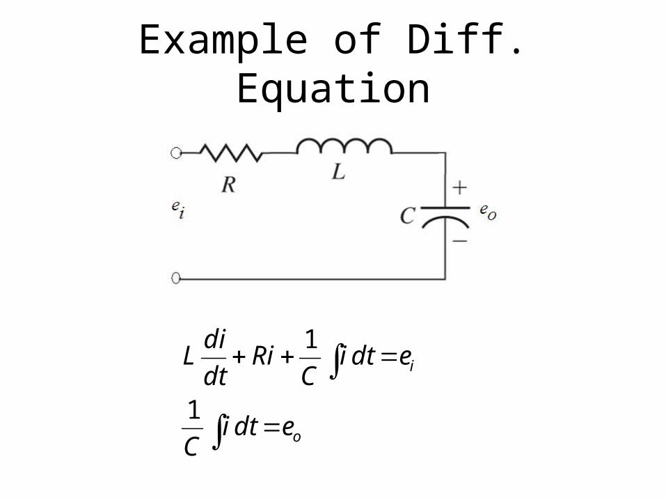
Example of Diff. Equation
o
i
edtiC
edtiC
Ridt
diL
1
1
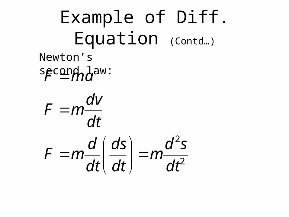
Example of Diff. Equation (Contd…)
Newton’s second law:
2
2
dt
sdm
dt
ds
dt
dmF
dt
dvmF
maF
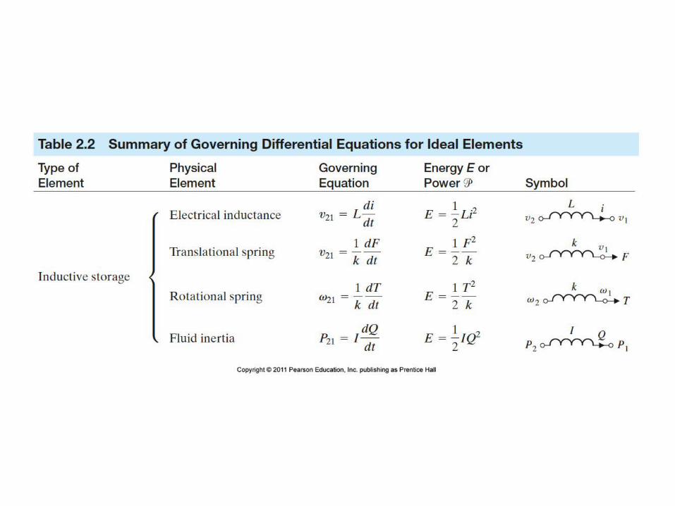
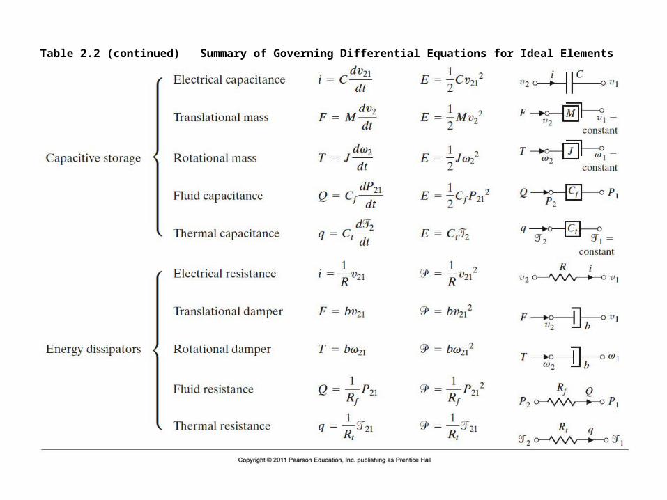
Table 2.2 (continued) Summary of Governing Differential Equations for Ideal Elements

Laplace Transform
• A transformation from time (t) domain to complex frequency (s) domain
Laplace Transform is given by
)}({)()(0
tfLdtetfsF st
frequency.complex a is Where, js
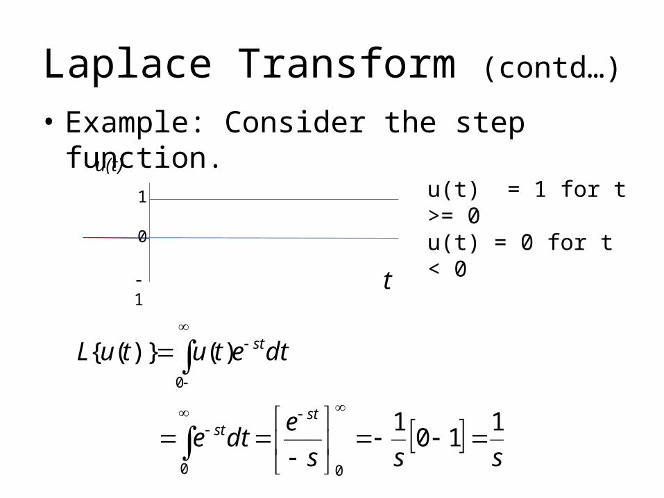
Laplace Transform (contd…)
• Example: Consider the step function.
t
u(t)
1
0
-1
sss
edte
dtetutuL
stst
st
110
1
)()}({
00
0
u(t) = 1 for t >= 0u(t) = 0 for t < 0
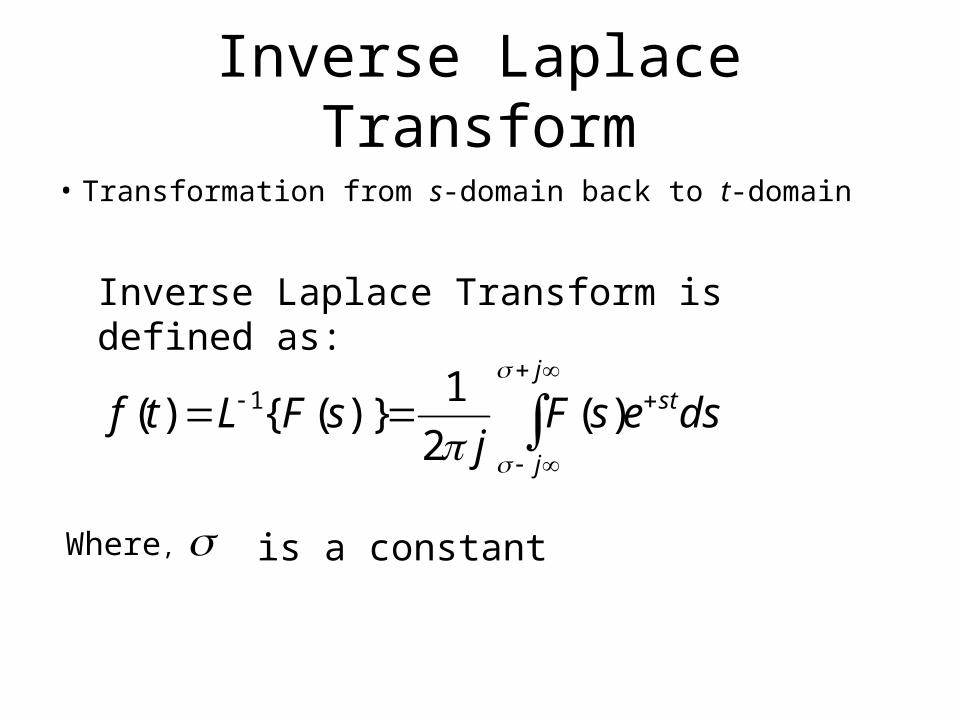
Inverse Laplace Transform
• Transformation from s-domain back to t-domain
Inverse Laplace Transform is defined as:
j
j
stdsesFj
sFLtf
)(
2
1)}({)( 1
Where, is a constant
Laplace Transform Pairs
• Laplace transform and its inverse are seldom calculated through equations.
• Almost always they are calculated using look-up tables.
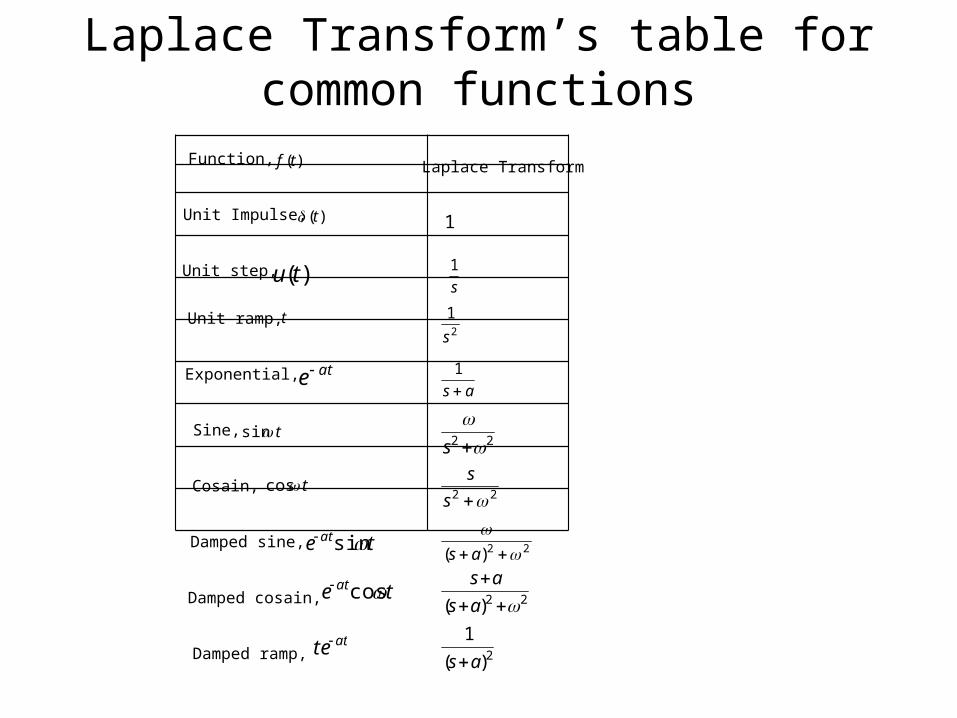
Laplace Transform’s table for common functions
Function, )(tf Laplace Transform
Unit Impulse, )(t 1
Unit step, )(tus
1
Unit ramp, t
Exponential, ate
Sine, tsin
Cosain, tcos
Damped sine, te at sin
Damped cosain, te at cos
Damped ramp, atet
2
1
s
as 1
22 s
22 s
s
22)(
as
22)( as
as
2)(
1
as
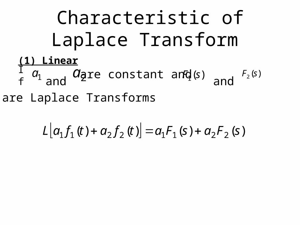
Characteristic of Laplace Transform
(1) Linear
1a 2a )(1 sF )(2 sFIf and are constant and and
are Laplace Transforms
)()()()( 22112211 sFasFatfatfaL
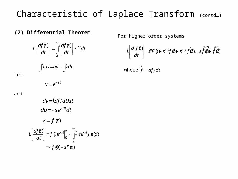
Characteristic of Laplace Transform (contd…)
(2) Differential Theorem
0
)()(dte
dt
tdf
dt
tdfL st
Let duvvudvu
steu
and
dtdtdfdv
dtesdu st .
)(tfv
)()0(
)()()(
00
ssFf
dttfseetfdt
tdfL stst
For higher order systems
)1()2(21 )0()0(.....)0()0()(
)(
nnnnn
n
n
ffsfsfssFsdt
tfdL
where dtdff
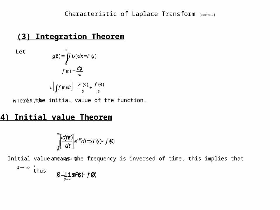
Characteristic of Laplace Transform (contd…)
(3) Integration Theorem
Let)()()(
0
sFdxxftg
dt
dgtf )(
s
f
s
sFdttfL
)0()()(
where )0(f is the initial value of the function.
(4) Initial value Theorem
)0()()(
0
fssFdtedt
tdf st
Initial value means 0t
and as the frequency is inversed of time, this implies that
s , thus)0()(lim0 fssF
s
Characteristic of Laplace Transform (contd…)
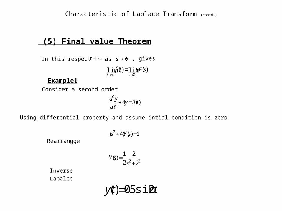
(5) Final value Theorem
t 0sIn this respect as , gives
)(lim)(lim0
ssFtfst
Example1Consider a second order
)(42
2
tydt
yd
Using differential property and assume intial condition is zero
1)()4( 2 sYsRearrangge
22 2
2
2
1)(
ssY
Inverse Lapalce
tty 2sin5.0)(
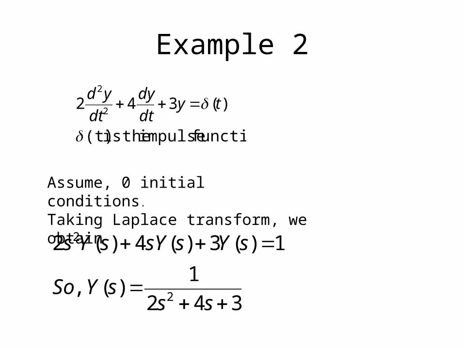
Example 2
function impulse theis (t)
)(3422
2
tydt
dy
dt
yd
Assume, 0 initial conditions.
Taking Laplace transform, we obtain
342
1)( ,
1)(3)(4)(2
2
2
sssYSo
sYssYsYs
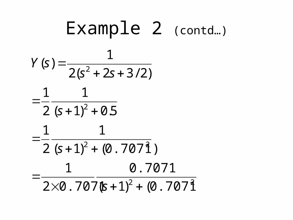
Example 2 (contd…)
22
22
2
2
0.7071)()1(
0.7071
0.70712
1
0.7071)()1(
1
2
1
5.0)1(
1
2
1
)2/32(2
1)(
s
s
s
sssY
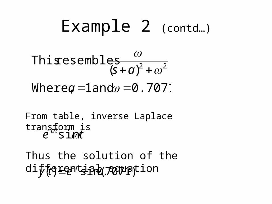
Example 2 (contd…)
0.7071 and 1 Where,
)( resembles This
22
a
as
From table, inverse Laplace transform is
te at sin
Thus the solution of the differential equation)7071.0sin()( tety t
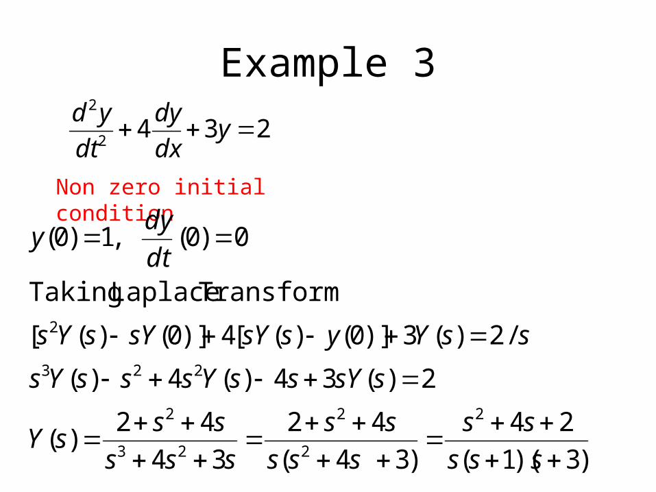
Example 3234
2
2
ydx
dy
dt
yd
Non zero initial condition
)3)(1(
24
)34(
42
34
42)(
2)(34)(4)(
/2)(3)]0()([4)]0()([
Transform Laplace Taking
0)0(,1)0(
2
2
2
23
2
223
2
sss
ss
sss
ss
sss
sssY
ssYssYsssYs
ssYyssYsYsYs
dt
dyy
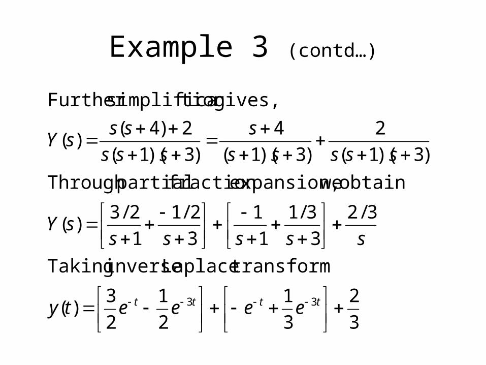
Example 3 (contd…)
3
2
3
1
2
1
2
3)(
transformLaplace inverse Taking
3/2
3
3/1
1
1
3
2/1
1
2/3)(
obtain weexpansion,fraction partialThrough
)3)(1(
2
)3)(1(
4
)3)(1(
2)4()(
gives,tion simplificaFurther
33
tttt eeeety
ssssssY
sssss
s
sss
sssY
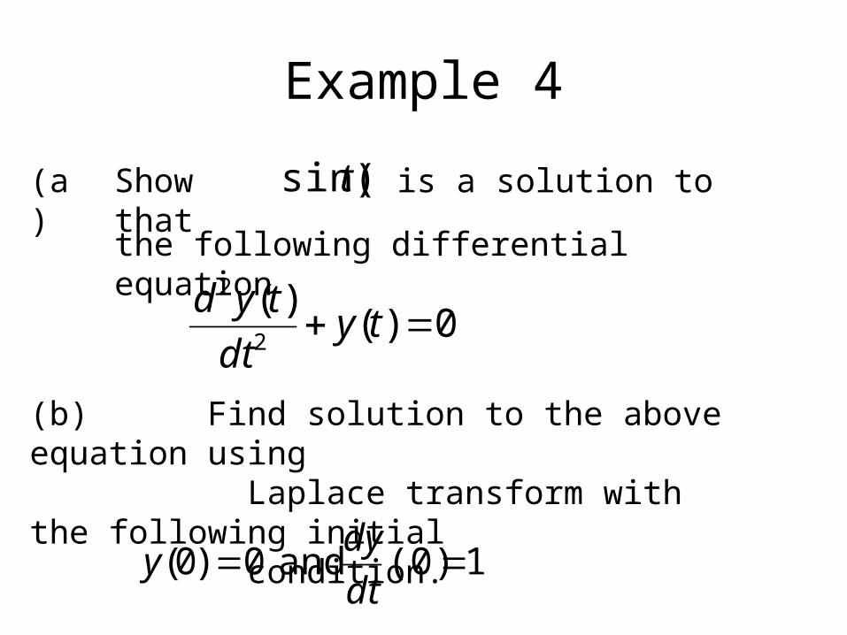
Example 4
Show that )sin(t is a solution to
the following differential equation
0)()(
2
2
tydt
tyd
(a)
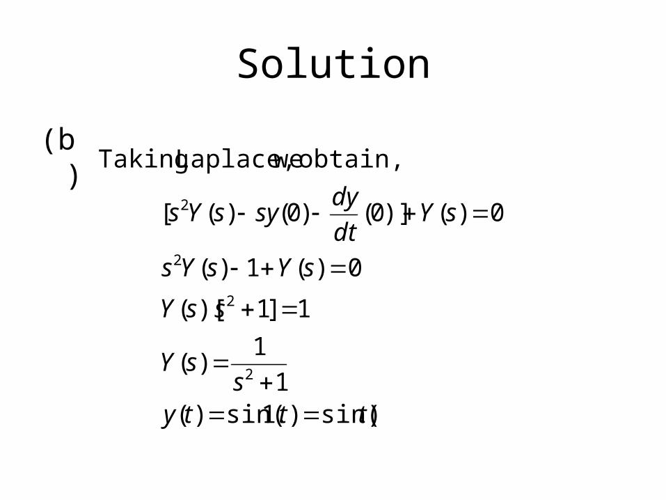
(b) Find solution to the above equation using Laplace transform with the following initial condition.
1(0) and 0)0( dt
dyy
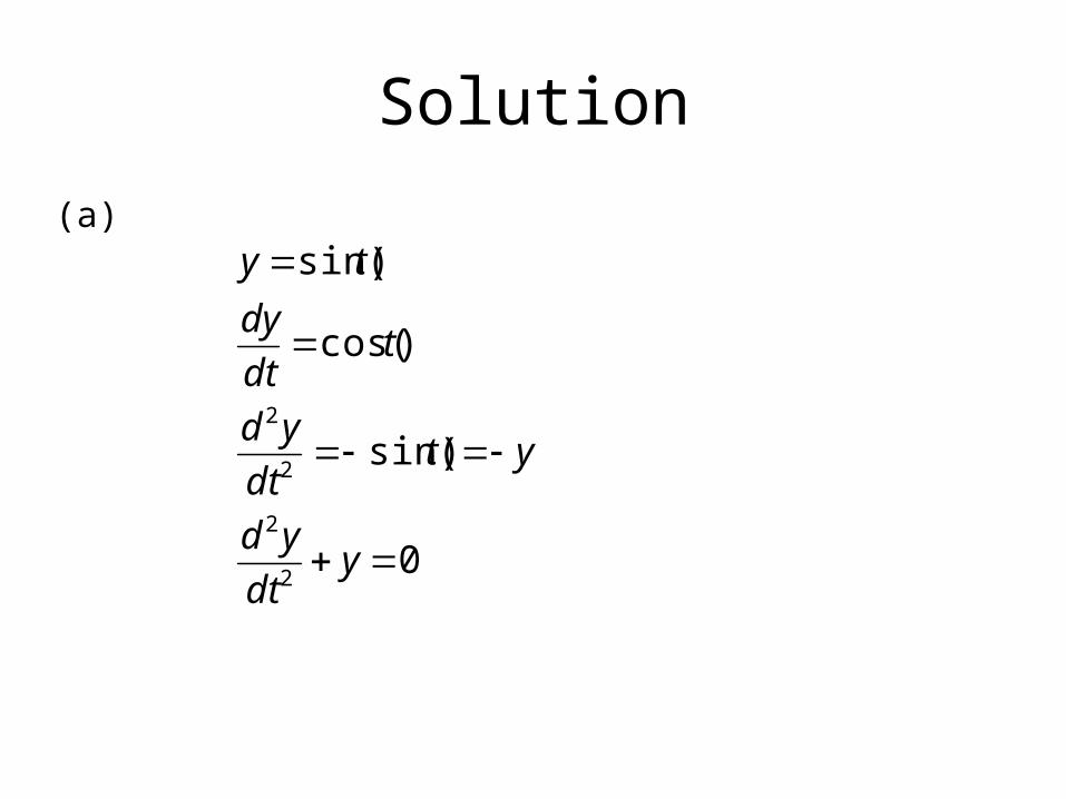
Solution
(a)
0
)sin(
)cos(
)sin(
2
2
2
2
ydt
yd
ytdt
yd
tdt
dy
ty
Solution
(b)
)sin().1sin()( 1
1)(
1]1)[(
0)(1)(
0)()]0()0()([
obtain, weLaplace, Taking
2
2
2
2
tttys
sY
ssY
sYsYs
sYdt
dysysYs