Federal Reserve Bank of Minneapolis Research Department Staff Report 376 August 2006

Modern Macroeconomics in Practice: How Theory Is Shaping Policy* V. V. Chari

University of Minnesota and Federal Reserve Bank of Minneapolis Patrick J. Kehoe

Federal Reserve Bank of Minneapolis and University of Minnesota ABSTRACT __________________________________________________________________________

Theoretical advances in macroeconomics made in the last three decades have had a major influence on macroeconomic policy analysis. Moreover, over the last several decades, the United States and other countries have undertaken a variety of policy changes that are precisely what macroeconomic theory of the last 30 years suggests. The three key developments that have shaped macroeconomic policy analysis are the Lucas critique of policy evaluation due to Robert Lucas, the time inconsistency critique of discre-tionary policy due to Finn Kydland and Edward Prescott, and the development of quantitative dynamic stochastic general equilibrium models following Finn Kydland and Edward Prescott. _____________________________________________________________________________________

*We thank Kathy Rolfe and Joan Gieseke for excellent editorial assistance. The views expressed herein are those of the authors and not necessarily those of the Federal Reserve Bank of Minneapolis or the Federal Reserve System.

Over the last three decades, macroeconomic theory and the practice of macroeconomics

by economists have changed significantly—for the better. Macroeconomics is now firmly

grounded in the principles of economic theory. These advances have not been restricted to the

ivory tower. Over the last several decades, the United States and other countries have undertaken

a variety of policy changes that are precisely what macroeconomic theory of the last 30 years

suggests.

The evidence that these theoretical advances have had a significant effect on the practice

of policy is often hard to see for policymakers and advisers who are involved in the hurly-burly

of day-to-day policymaking, but easy to see if one steps back and takes a longer-term perspec-

tive. Examples of the effects of theory on the practice of policy include increased central bank

independence, adoption of inflation targeting and other rules to guide monetary policy, increased

reliance on consumption and labor taxes instead of capital income taxes, and increased aware-

ness of the costs of policies that distort labor markets.

Three key developments in academic macroeconomics have shaped macroeconomic pol-

icy analysis: the Lucas critique of policy evaluation due to Robert Lucas (1976), the time incon-

sistency critique of discretionary policy due to Finn Kydland and Edward Prescott (1977), and

the development of quantitative dynamic stochastic general equilibrium models following Finn

Kydland and Edward Prescott (1982).1 Lucas argued that economic theory implies that prefer-

ences and technology are invariant to the rule describing policy but that decision rules describing

private agents’ behavior are not. In a series of graphic examples, he showed that then standard

policy analyses which presumed invariance of decision rules lead to dramatically undesirable

policy prescriptions. Kydland and Prescott argued that a regime in which policymakers set state-

2

contingent rules once and for all is better than a discretionary regime in which policymakers se-

quentially choose policy optimally given their current situation.

The practical effect of the Lucas critique is that both academic and policy-oriented ma-

croeconomists now take policy analyses seriously only if they are based on quantitative general

equilibrium models in which the parameters of preferences and technologies are reasonably ar-

gued to be invariant to policy. The time inconsistency critique has been a major influence on the

practice of central banking and fiscal policymaking over the last 30 years.

The quantitative general equilibrium models that were developed in response to the Lucas

critique have become increasingly sophisticated over time, including models with financial mar-

ket imperfections, sticky prices and other monetary nonneutralities, imperfect competition, in-

complete markets, and other frictions. (See Cooley, 1995.) These models have yielded four ro-

bust properties of optimal monetary and fiscal policies under commitment:

1. Monetary policy should be conducted so as to keep nominal interest rates and inflation

rates low.

2. Tax rates on labor and consumption should be roughly constant over time.

3. Capital income taxes should be roughly zero.

4. Returns on debt and taxes on assets should fluctuate to provide insurance against adverse

shocks.

Macroeconomists have also been profitably applying the basic tools of general equilib-

rium theory, computational techniques, and a deep understanding of key features of the data to a

wide area of phenomena outside of narrowly defined macroeconomics. These include income

differences across countries, fertility behavior across time and countries, the dynamics of the size

distribution of firms, and the efficiency costs of the welfare state. A good illustration of this kind

3

of work is the study of differences in labor market performance between the United States and

Europe. Although work of this kind has not yet directly affected policy, it will once its policy

lessons, carefully grounded in theory and data analysis, are clearly communicated to policymak-

ers and the public.

Here we have focused on the role of theory shaping policy. In practice, of course, causal-

ity runs in both directions. Theorists often work on problems motivated by specific policy ques-

tions and specific experiences. Policymakers’ mind-sets and attitudes are influenced, perhaps

subconsciously, by apparently remote developments in theory. Nevertheless, the most straight-

forward reading of developments in macroeconomic policy is that they were strongly influenced

by developments in macroeconomic theory.

Modern Theoretical Developments

Expectations and Macroeconomic Policy Analysis

The Lucas critique led economists to understand that people’s decision rules change

when the way policy is conducted changes. Lucas (1976) forcefully argued that the question

“How should policy be set today?” was ill-posed. In most situations, people’s current decisions

depend on their expectations of what future policies will be. Those expectations depend, in part,

on how people expect policymakers to behave. Macroeconomists now agree, therefore, that any

sensible policy analysis must include a clear specification of how a current choice of policy will

shape expectations of future policies.

To see more concretely why analyzing policy requires specifying how policy will be set

in the future, consider two examples. First, consider a monetary authority deciding on monetary

policy for today. This authority needs to forecast how variables such as inflation and output will

behave now and in the future, which means that it must forecast private behavior in the future.

4

But the decisions of private actors depend on their expectations about future monetary policy. If

private actors expect tight monetary policy in the future, they will react to current price and wage

pressures in one way; if they expect to lose monetary policy in the future, they will react differ-

ently. Thus, the monetary authority cannot predict how the economy will respond to a policy de-

cision today unless it can also predict how people’s expectations of future monetary policy will

change as a result of the current decisions. The monetary authority also needs to predict how its

own behavior will change in the future as a result of its current actions.

Next, consider a fiscal authority deciding how to tax capital income. This authority needs

to forecast how output, investment, and other variables will respond to its decisions. Investment

decisions, for example, depend on investors’ expectations of future tax rates. If investors expect

future tax rates to be low, then they’ll invest more today; if high, then less today. Consequently,

the fiscal authority cannot predict how investment will respond, for example, to a tax cut today

unless it knows how people’s expectations of future tax rates will change as a result of the cut.

The fiscal authority also needs to predict how its own future behavior will change as a result of

its current actions.

With this concern over expectations in mind, macroeconomists now agree that a coherent

framework for the design of economic policy consists of three parts: a model to predict how peo-

ple will behave under alternative policies, a welfare criterion to rank the outcomes of alternative

policies, and a description of how policies will be set in the future.

A commitment regime is the easiest environment to describe how future policies are set.

In such a regime, all policies for today, tomorrow, the day after, and so on are set today and can-

not be changed. These policies could be contingent on various events that might occur in the fu-

ture. The model can then be used to predict the consequences of various plans for policy and can

5

be used to find the optimal plan. This procedure has its origins in the public finance tradition

stemming from Ramsey (1927), so this sequence of optimal policies is referred to as Ramsey

policies and their associated outcomes as Ramsey outcomes.

Time Inconsistency Problem

The Lucas (1976) critique addressed situations in which expectations of future policies

affect current decisions. The Lucas critique thus leads naturally to thinking about policy evalua-

tion as comparing alternative sets of rules that describe policy both now and in the future. In

practice, of course, societies may not be able to commit to future policies. In a series of graphic

examples, Kydland and Prescott (1977) (soon followed by Calvo, 1978; Fischer, 1980) analyzed

policies with and without commitment and showed that Ramsey policies are often time inconsis-

tent; that is, outcomes with commitment are different from those without commitment. Their ex-

amples suggest that time inconsistency problems arise when people’s current decisions depend

on expectations of future policies. Since people’s decisions have been made by the time the fu-

ture date arrives, the government often has an incentive to renege on the Ramsey policies.

To better understand this problem, consider again examples from monetary and fiscal

policy. The monetary policy example is motivated by the work of Kydland and Prescott (1977)

and Barro and Gordon (1983). Assume that at the beginning of each period, wage setters choose

nominal wages so as to attain a target level of real wages. The monetary authority then chooses

the inflation rate. If inflation is higher than wage setters expected, then real wages are lower than

the target level, firms demand more labor, and output is higher than its natural rate (which is its

level when real wages are at their target level). The monetary authority wants to maximize soci-

ety’s welfare, which is increasing in output and decreasing in inflation. As output increases, the

natural assumption is that the marginal benefits of increases in output fall because of diminishing

6

marginal utility. We assume in addition that as inflation increases, the marginal costs of increases

in inflation rise. This assumption holds in many general equilibrium models.

To see that there is a time inconsistency problem in this setup, consider the best outcomes

under commitment, the Ramsey outcomes. We think of commitment as a situation in which at

the beginning of time society prescribes a rule for the conduct of monetary policy in all periods.

The monetary authority then simply implements the rule. The best rule under commitment pre-

scribes zero inflation in all periods. Under this rule, real wages are equal to their target level. To

see why zero inflation is optimal, consider a rule that prescribes positive inflation. Wage setters

anticipate positive inflation and set their nominal wages to be appropriately higher. Under this

policy, real wages are still at their target level, output is unaffected, but inflation is positive.

Clearly this outcome is worse than one under a policy that prescribes zero inflation.

Consider next outcomes with no commitment. We think of no commitment as a situation

in which in each period the monetary authority chooses policy optimally given the nominal

wages that wage setters have already chosen. In the resulting outcome, called the static discre-

tionary outcome, inflation is necessarily positive while output is at its natural rate. To see why

inflation is necessarily positive, suppose, by way of contradiction, that inflation rates are zero so

that wage setters set their wages anticipating zero inflation. Once the nominal wages are set,

however, the monetary authority will deviate and generate inflation in order to raise output.

Hence, inflation must be positive. To see why output is at its natural rate, note that wage setters

rationally anticipate the actions of the monetary authority so that real wages are at their target

level. In the static discretionary outcome, inflation is at a high enough level so that the marginal

cost of deviating to an even higher inflation rate is equal to the marginal benefit of increased

output.

7

In the case of fiscal policy, a good example of the time inconsistency problem is based on

Kydland and Prescott (1977). Consider a model in which the government needs to raise revenue

from proportional taxes on capital and labor income to finance a given amount of government

spending. Under commitment, society chooses a rule for setting tax rates in all periods, and the

fiscal authority implements the rule. At any instant, the stock of capital is given by past invest-

ment decisions; however, the supply of labor can be changed relatively quickly. The key influ-

ence on investment decisions that determine the capital stock in the future is the after-tax return

expected in the future, whereas the key influence on labor supply decisions is the current after-

tax wage rate. So the government’s best policy for current tax rates is to tax capital at high rates

and labor at low rates. This policy does not distort capital supply decisions, since the capital

stock is fixed and irreversible in that capital goods cannot be directly converted into consumption

goods. The policy also ensures that labor supply is not distorted much, since the tax rates on la-

bor are low. For future tax rates, the best policy is to commit to set low rates on capital to stimu-

late investment and to raise the rest of the needed revenue with higher rates on labor.

Consider next the outcomes with no commitment. In each period, the fiscal authority still

has an incentive to tax capital income heavily, since the capital stock is fixed, and to tax labor in-

come lightly to avoid distorting labor supply. Without commitment, however, investors today ra-

tionally expect that high taxes on capital income will continue into the future—since such taxes

are preferred in each time period—and investment will be low. In equilibrium, the capital stock

is smaller than it would be under commitment, and both output and welfare are correspondingly

lower than they would be under commitment.

The message of examples like these is that discretionary policymaking has only costs and

no benefits, so that if government policymakers can be made to commit to a policy rule, society

8

should make them do so. Our examples have no shocks. In stochastic environments the optimal

policy rule is contingent on the shocks that affect the economy. A standard argument against

commitment and for discretion is that specifying all the possible contingencies in a rule made

under commitment is extremely difficult, and discretion helps policymakers respond to unspeci-

fied and unforeseen emergencies. This argument is less convincing than it may seem. Every pro-

ponent of rule-based policy recognizes the necessity of escape clauses in the event of unforeseen

emergencies or extremely unlikely events. These escape clauses will, of course, reintroduce a

time inconsistency problem, but in a more limited form. Almost by definition, deviations from

such rules will occur rarely; hence, the time inconsistency problem arising from the escape

clauses will be small. Commitment to a rule with escape clauses is not unworkable.

What can be done to ameliorate the time inconsistency problem short of commitment? A

superficially attractive approach is to pass legislation requiring the monetary or the fiscal author-

ity to abide by rules. This approach is more problematic than it may seem. In most macroeco-

nomic environments with time inconsistency problems, given an initially established rule, all

members of society (or a large majority) would like to deviate from it. Legislatures will have a

strong incentive to allow the monetary or fiscal authority to deviate from the established rule. To

be effective, therefore, attempts to ameliorate the time inconsistency problem must impose costs

on policymakers of deviating from the earlier agreed-upon rules.

The most widely studied ways to impose such costs rely on either reputation or trigger

strategy mechanisms. Such mechanisms can lead to better outcomes under discretion than the

static discretionary outcomes. Indeed, if policymakers discount the future sufficiently little, these

mechanisms can lead policymakers to choose the Ramsey outcomes.

9

Our illustration of such mechanisms draws on Chari, Kehoe, and Prescott’s (1989) analy-

sis of the Kydland and Prescott (1977) and Barro and Gordon (1983) monetary policy example.

Consider the following trigger strategy mechanism in an infinite horizon version of this example.

In this mechanism, as long as the monetary authority has chosen the Ramsey policies in the past,

wage setters expect it to continue to do so; however, if the monetary authority has ever deviated

from the Ramsey policies, wage setters expect it to choose the static discretionary policies for-

ever in the future. With these beliefs of private agents, the monetary authority understands that if

it unexpectedly inflates, it gets a current gain from the associated rise in output but a loss in all

future periods equal to the difference in welfare between the static discretionary outcome and the

Ramsey outcome. In this situation, if the monetary authority discounts the future sufficiently lit-

tle, then it will not deviate. Although the use of trigger strategy mechanisms is appealing, one

difficulty is that many outcomes can result from trigger strategies, and how society will coordi-

nate on a good outcome is not obvious.

Another device for ameliorating the time inconsistency problem is to delegate policy to

an independent authority (Rogoff, 1985). One notion of what it means for an authority to be in-

dependent is that society faces large costs to dismiss the authority and replace it with another.

We illustrate this device in the Kydland and Prescott (1977) monetary policy example, modified

to include potential policymakers who differ in terms of their aversion to inflation. Suppose the

appointed policymaker is extremely averse to inflation. After wage setters have chosen their

nominal wages, this policymaker finds engineering a surprise inflation very costly. Wage setters

anticipate this behavior, and the outcome is low inflation and output at its natural rate.

Note that if dismissing the authority is not costly, the delegation device is not effective.

The authority will be dismissed after wage setters have set their nominal wages, and an authority

10

more representative of society will be appointed. Wage setters will anticipate this behavior, and

the outcomes will simply be the static discretionary outcomes. Making it costly to dismiss the au-

thority essentially makes it costly for society to deviate from some set of rules and, hence, intro-

duces a specific form of commitment.

Yet another device for ameliorating the time inconsistency problem is to set up institu-

tions that ensure that policies cannot be implemented until several periods after they are chosen.

To see the advantage of such implementation lags, recall the fiscal policy example. There, with-

out commitment, the optimal policy is to set the tax rate of capital income high, since the capital

stock is determined entirely by past investment decisions, and to set the tax rate on labor income

low, since labor supply decisions are determined primarily by current tax rates. Suppose that the

fiscal authority still chooses tax rates on capital and labor income, but that now these tax rates

can only be implemented several periods after they are chosen. Under such institutions, choosing

a high tax rate on capital income will tend to reduce investment, at least until the implementation

date, and will lead to a corresponding reduction in the capital stock. In this environment, the de-

lay in implementation means that policymakers are forced to confront at least part of the distor-

tions arising from high capital taxation.

Optimal Rules and Monetary Policy

Macroeconomists can now tell policymakers that to achieve optimal results, they should design

institutions that minimize the time inconsistency problem by promoting a commitment to policy

rules. However, to what particular policies should policymakers commit themselves? For many

macroeconomists considering this question, quantitative general equilibrium models have be-

come the workhorse model, and they turn out to offer surprisingly sharp answers. Macroecono-

mists now generally agree on four properties that optimal policies should have and on when

11

qualifications of those properties are appropriate. One of the four properties applies to monetary

policy; the other three, primarily to fiscal policy.

Optimal Rules for Monetary Policy

In the area of monetary policy, the optimal rule is to set policy so that nominal interest

rates and inflation will be low. This result is due to the celebrated work of Milton Friedman

(1969), which it has been defended and supplemented by more recent work based on standard

public finance principles.

Friedman’s argument stems from an analysis of the forces determining money-holding

decisions. Money has benefits to individuals and therefore to society by reducing the costs of

making transactions. From each individual’s perspective, the opportunity cost of money is the

forgone nominal interest that could be obtained by investing it instead. From society’s perspec-

tive, the opportunity cost of producing money is close to zero. Thus, society should conduct

monetary policy so that the nominal interest rate equals the opportunity cost of producing money

and is therefore close to zero. This recommendation for monetary policy is known as the Fried-

man rule. (This rule should not be confused with a k-percent rule for monetary aggregates also

advocated by Friedman.) This recommendation holds in both deterministic and stochastic envi-

ronments.

An alternative way to implement the Friedman rule is to pay interest on money. Although

it may be technologically difficult to pay interest on currency, it is possible to pay interest on

checking accounts and other means of making transactions. This reasoning suggests that elimi-

nating policies that limit interest payments on demand deposits, such as Regulation Q, move us

closer to the Friedman rule.

12

Phelps (1973) made what looked at first like a compelling argument that a nominal inter-

est rate close to zero is unlikely to be optimal in practice. He noted that if government revenue

must be raised through distorting taxes, the optimal policy is actually to tax all goods, including

the liquidity services derived from holding money, so that the optimal interest rate is substan-

tially greater than zero. Chari, Christiano, and Kehoe (1996) showed, however, that for a class of

economies consistent with the growth facts on the absence of long-term trends in the ratio of out-

put to real balances, a nominal interest rate close to zero is in fact optimal, even if government

revenue must be raised through distorting taxes. For such economies, money acts like an inter-

mediate good, and for well-known public finance reasons, taxing intermediate goods is not opti-

mal.

An intuitive way to think about the Friedman rule’s prescription that the nominal interest

rate be zero is that it prescribes that the risk-adjusted real rate of return on money should be the

same as the (risk-adjusted) real rate of return on other assets. In a deterministic environment no

risk adjustments are needed, so that the Friedman rule implies deflation at the real interest rate.

Some economists have interpreted the Friedman rule as always requiring deflation at the real in-

terest rate. Chari, Christiano, and Kehoe (1996), however, showed that this interpretation is mis-

taken by showing that in a plausible parameterized stochastic environment, even though the op-

timal nominal interest rate is still zero, there is no deflation. Indeed, under the optimal policy the

inflation rate is roughly zero because money turns out to be a hedge against real fluctuations,

paying out relatively more in bad times and relatively less in good times. Indeed, money turns

out to be enough of a hedge so that even at zero inflation, its risk-adjusted real rate of return

equals that on other assets.

13

We turn now to some qualifications. In some well-known macroeconomic models, posi-

tive nominal interest rates are optimal. Typically, in these models, if the government had a rich

enough set of fiscal instruments, then a zero nominal interest rate would be optimal, but positive

nominal interest rates can make sense if the set of instruments available to the government is re-

stricted.

Positive nominal interest rates are optimal in sticky price models with nominal prices or

wages set in a staggered fashion and in which the government is restricted to uncontingent nomi-

nal debt and uncontingent consumption taxes. Absent such stickiness, even when the government

is so restricted, zero nominal interest rates are optimal and volatile inflation is used to make

nominal debt mimic real state contingent debt (Chari, Christiano, and Kehoe, 1991). If nominal

prices or wages are set in a staggered fashion, then such inflation volatility is costly because fluc-

tuations in inflation induce undesirable fluctuations in relative prices. In this setting, optimal

monetary policy trades off two desirable goals. One is to maintain price stability to avoid the

misallocations induced by fluctuations in relative prices. The other goal is to minimize the social

waste of using inefficient methods of conducting transactions. Not surprisingly in this setting,

optimal monetary policy involves a compromise between positive interest rates to reduce infla-

tion and promote price stability and a nominal interest rate of zero (Benigno and Woodford,

2003; Khan, King and Wolman, 2003; Siu, 2004; Schmitt-Grohé and Uribe, 2004). The undesir-

able fluctuations in relative prices can be avoided if either state-contingent debt or state-

contingent consumption taxes are available (Correia, Nicolini, and Teles, 2004).

Another set of environments in which positive nominal interest rates are optimal has a re-

stricted set of assets available to share risk among individuals. In this setting, lump-sum transfers

financed by printing money redistribute income from the temporarily rich to the temporarily

14

poor. The reason is that inflation imposes a larger tax on those who hold more money and, in this

setting, households who hold more money are the temporarily rich. Such transfers provide a form

of risk sharing and therefore help raise welfare. Optimal monetary policy trades off the benefits

of risk sharing against the social waste of using inefficient methods of conducting transactions,

and that involves a positive nominal interest rate (Levine, 1991). Here, also, a rich enough set of

fiscal policy instruments can provide a partial remedy, risk sharing, and allow the monetary au-

thority to follow the Friedman rule (da Costa and Werning, 2003).

Thus, modern macroeconomic theory argues that positive nominal interest rates are opti-

mal only if the set of instruments available to the government is restricted. Since this situation is

highly likely in practice, optimal monetary policy involves a compromise between the goals of

zero nominal interest rates and other goals. The robust finding is not that nominal interest rates

should be literally zero but that nominal interest rates and inflation rates should be low.

The practical definition of low interest rates and inflation rates is a subject of continuing

discussion, particularly because of biases in measuring inflation rates due to quality changes. Al-

though no consensus has emerged on the definition of low inflation, most macroeconomists

agree that a sustained inflation in excess of 3 percent per year is unacceptably high.

The Evolution of Monetary Policy

Over the last three decades, a variety of specific monetary policy proposals consistent

with macroeconomic theory’s developments have been debated and implemented around the

world. Central bankers and other monetary policymakers have begun to concentrate on price sta-

bility and inflation control as their main objectives. Many countries have changed their institu-

tional frameworks for monetary policymaking in an apparent recognition of the time inconsis-

tency problem. These changes have emphasized the importance of characteristics key to mini-

15

mizing that problem—credibility, transparency, and accountability—as well as clear statements,

or rules, about the objectives of monetary policy and the methods by which that policy will re-

spond to varying circumstances. All these changes point to a shift in the world toward the rule-

based method of policymaking which is prescribed by modern macroeconomic theory.

Two kinds of institutional changes are especially evident in the practice of monetary pol-

icy. Central banks have become substantially more independent of the political authorities, and

to an increasing extent, the charters of central banks have emphasized the primacy of inflation

targeting and price stability.

An extensive empirical literature has argued that central bank independence helps reduce

inflation rates without any adverse consequences on output. Figure 1, which reproduces Figure

1A from Alesina and Summers (1993), shows that countries with more independent central

banks tend to have lower inflation rates. Alesina and Summers (1993) also show that countries

with more independent central banks do not suffer in terms of output performance. One interpre-

tation of these findings is that institutions that promote central bank independence ameliorate the

time inconsistency problem. Under this interpretation, the findings in the literature support the

key feature of the Kydland and Prescott (1977) example: reducing the time inconsistency prob-

lem ameliorates inflation but has no effect on output.

Bernanke et al. (1999) have argued that inflation targeting is moving toward a rule-based

regime. Their idea (p. 24) is that “inflation targeting requires an accounting to the public of the

projected long run implications of its short run policy actions.” This accounting can help amelio-

rate the time inconsistency problem by ensuring that the long-run implications of short-run pol-

icy actions are explicitly taken into account in the policymaking process.

16

In practice, inflation targeting often involves setting bands of acceptable inflation rates.

(See, for example, Bernanke and Mishkin 1997.) In theoretical models without private informa-

tion, optimal policy does not involve setting bands, but rather involves specifying exactly what

the monetary authority should do in every state. In this sense, such models imply that the mone-

tary authority should have no discretion. Athey, Atkeson, and Kehoe (2005) construct a model in

which the monetary authority has private information about the economy and show that the op-

timal policy allows for limited discretion in that it specifies acceptable ranges for inflation and

gives the monetary authority complete discretion within those ranges. In this way, Athey, At-

keson, and Kehoe provide a theoretical rationale for the type of inflation targeting often seen in

practice.

Perhaps the most vivid example of both the movement toward independence and the

movement toward a rule-based method of policymaking is to be found in the charter of the Euro-

pean Central Bank (ECB). Article 105 of the treaty establishing the central bank states that “the

primary objective” of the European System of Central Banks (ESCB) shall be to “maintain price

stability.” Article 107 of the treaty emphasizes and protects the independence of the central bank

by mandating that “neither the ECB, nor a national central bank, nor any member of their deci-

sion-making bodies shall seek or take instructions from Community institutions or bodies, from

any government of a Member State or from any other body.” Furthermore, the Maastricht Treaty

and the Stability and Growth Pact contain provisions restricting fiscal policies in the member

countries in order to make the pursuit of price stability easier.2 The change in the conduct of

European monetary policy is especially marked for countries other than Germany in the Euro-

pean monetary union.

17

Over the last 20 years, monetary policy in the United Kingdom has also moved in the di-

rection of greater independence as well as toward rule-based policymaking. After experiencing a

major exchange rate crisis, the United Kingdom adopted a form of inflation targeting in October

1992. In May 1997 (and subsequently formalized by the Bank of England Act of 1998), the Bank

of England gained operational independence from the government. The Bank of England is now

specifically required primarily to pursue price stability and only secondarily to make sure that its

policies are consistent with the growth and employment objectives of the government. The gov-

ernment periodically sets an inflation target, currently 2 percent, and the central bank is given

broad freedom in achieving this target. As part of the inflation target, the government also sets

ranges for acceptable fluctuations in inflation. If inflation moves outside its target range, the cen-

tral bank is required to report on the causes for this deviation, the corrective policy action the

central bank plans to take, and the time period within which inflation is expected to return to its

target range.

The movement toward rule-based monetary policy is widespread. By 2002, 22 countries

had adopted monetary frameworks that emphasize inflation targeting (Truman, 2003). The fol-

lowing countries are listed by the date in which inflation targeting was adopted (and in some

cases readopted): in 1989, New Zealand; in 1990, Chile; in 1991, Canada and Israel; in 1992, the

United Kingdom; in 1993, Australia, Finland, and Sweden; in 1995, Spain and Mexico; in 1997,

Czech Republic and Israel (again); in 1998, Poland and Korea; in 1999, Brazil, Chile (again),

and Colombia; in 2000, Thailand and South Africa; in 2001, Hungary, Iceland, and Norway; in

2002, Peru and the Philippines. These countries have all openly published their inflation targets

and have described their monetary framework as one of targeting inflation. Clearly, inflation tar-

18

geting is worldwide; the countries range from developed economies to emerging market econo-

mies. The number of countries adopting targeting inflation is growing over time.

The first country to adopt inflation targeting, New Zealand, has gone the furthest in set-

ting up a rule-based regime. Before 1989, monetary policy in New Zealand was far from being

rule-based. As Nicholl and Archer (1992, p. 316) describe:

New Zealand experienced double digit inflation for most of the period since the first oil

shock. Cumulative inflation (on a Consumer Price Index (CPI) basis) between 1974 and

1988 (inclusive) was 480 percent. . . . Throughout the period, monetary policy faced mul-

tiple and varying objectives which were seldom clearly specified, and only rarely consis-

tent with achievement of inflation reduction.

In 1989, the government of New Zealand adopted legislation mandating that the objective of the

central bank be to maintain a stable general level of prices. The government and the governor of

the central bank must agree to a policy target, which specifies an acceptable range for inflation.

Since the act was adopted, the inflation rate has fallen considerably and has been well below 5

percent per year over the last decade or so.

Figure 2 displays the inflation experiences for four countries—the United Kingdom, New

Zealand, Canada, and Sweden—that have adopted inflation targeting. The four panels of Figure

2 show the inflation rates before and after the date of the inflation targeting regime, marked by a

vertical line. The bands in the figure following the adoption of the inflation targeting regime de-

pict ranges of inflation as specified in the regime. Although the countries did not always remain

within the target range for inflation after adopting inflation targeting, inflation fell substantially

in all the countries after the adoption of inflation targeting. The literature contains ongoing con-

19

troversy about whether this decline was solely due to inflation targeting, but also offers substan-

tial consensus that inflation targeting played an important role in the decline.

Even in countries that have not explicitly adopted inflation targeting, the institutional

framework for the conduct of monetary policy has changed in a way consistent with modern

macroeconomic theory. In the United States, for example, the central bank has been moving to-

ward openness and targeting for the last 25 years. The Full Employment and Balanced Growth

Act of 1978 (commonly referred to as the Humphrey-Hawkins Full Employment Act) required

the Federal Reserve Board of Governors to report periodically to Congress on the planned course

of monetary policy. Furthermore, the Federal Reserve Board has changed some policies in ways

that increase transparency. For example, the minutes of Federal Open Market Committee

(FOMC) meetings are now released substantially sooner than they used to be, and the FOMC’s

decisions regarding its interest rate target are now released immediately after the meeting. A

large academic literature motivated by Taylor (1993) has argued that the Fed has effectively

moved toward a rule-based regime and is therefore well placed to solve the time inconsistency

problem.

Although the changes in the practice of monetary policy documented above cannot be de-

finitively linked to the recent theoretical developments in macroeconomics, the most straightfor-

ward explanation for these changes is that they are due to the identification of the time inconsis-

tency problem by macroeconomic theorists.

Optimal Rules and Fiscal Policy

The macroeconomics and public finance literature on proportional tax systems is based on an

analysis that taxes distort two key types of decisions: the static trade-off between consumption

and leisure and the intertemporal trade-off between current and future consumption.

20

Taxes on both labor income and consumption distort the static trade-off. When people

contemplate working for an extra hour in the market, they balance the disutility of the extra work

against the utility from the extra consumption they will have as a result. An extra hour of work at

pre-tax wage w yields extra after-tax income of (1 )l w− τ and allows additional after-tax con-

sumption of (1 ) /(1 )l cw− τ + τ , where lτ is the tax rate on labor income and cτ is the tax rate on

consumption. This balancing act implies that the distortion of taxes on the labor supply is sum-

marized by the tax-induced labor wedge ,τ defined so that 1 (1 ) /(1 ).l c− τ = − τ + τ Notice that

consumption taxes distort the static trade-off in much the same way as do taxes on labor income.

A tax on capital income reduces the return to savings and clearly distorts the intertempo-

ral trade-off. A constant capital income tax can easily be shown to be equivalent to an increasing

sequence of consumption taxes. A pattern of consumption taxes that rise over time raises the

price of future consumption relative to current consumption and therefore also distorts the in-

tertemporal trade-off. Interestingly, constant consumption taxes do not change the relative price

of consumption over time and thus do not distort the intertemporal trade-off.

Principles and Properties of Optimal Tax Systems

The problem of designing optimal fiscal policy is to raise the needed amount of revenue

while distorting the static and the intertemporal trade-offs as little as possible. Studies of optimal

fiscal policy have argued that optimal policies should be based on two principles. First, similar

goods should be taxed at similar rates. More specifically, the consumption of commodities that

enter preferences and production technologies in similar ways should be distorted in similar

ways. Second, if preferences are homothetic in commodities and separable from labor, then all

commodities should be taxed at a uniform rate.

21

These principles can be applied to dynamic stochastic economies, such as those com-

monly modeled in the macroeconomics literature, by reinterpreting each commodity as the con-

sumption good at a different date and state. The first principle—similar goods, similar taxes—

implies that the optimal policy is to distort the static trade-off in the same way at all dates and

states. To apply the second principle, note that in most quantitative general equilibrium models,

preferences are assumed to be homothetic in consumption at different dates and separable from

labor. Since uniform commodity taxation is optimal with these assumptions, it follows that the

intertemporal trade-off should not be distorted.

In dynamic stochastic environments, one tax system that is consistent with these princi-

ples and with the requirement that the present value of the government budget be balanced at

each state has three properties. First, tax rates on labor and consumption should be roughly con-

stant over time. Second, capital income taxes should be roughly zero. Third, returns on debt and

taxes on assets should fluctuate so as to balance the government’s budget in a present value sense

at each state.

To see how the first two properties follow from the principles, note that when labor and

consumption tax rates are constant, the static trade-off is distorted in the same way in all dates

and states. When capital income taxes are zero, the intertemporal trade-off is not distorted.

The third property follows from the requirement that the government budget stay bal-

anced in a present value sense and is a useful feature of dynamic stochastic models: the intertem-

poral trade-off does not depend on the pattern of returns on debt and taxes across states but only

on an appropriately weighted average of taxes across states. To maintain the government budget

balance while keeping tax rates on labor and consumption constant in a stochastic environment

and not distorting the intertemporal trade-off, some other source of revenue must fluctuate. Ap-

22

propriately designed state-contingent returns on debt or state-contingent taxes on assets are such

a source of revenue. To see how state-contingent returns on debt can be such a source of reve-

nue, consider a policy that issues debt with low returns when revenue needs are high and issues

debt with high returns when revenue needs are low. This policy can ensure that the government

budget is balanced in a present value sense at each state even though taxes on consumption, labor

income, and capital income are roughly the same both across time and states. Note that under this

policy, the government is insuring itself against fluctuations in revenues and expenditures.

One concern raised with this analysis is that state-contingent government debt is rarely

observed in practice. But this concern is exaggerated because there are several ways to implicitly

make returns on government debt state-contingent. One is to issue nominal debt and let inflation

rates be high when revenue needs are high and low when revenue needs are low. Under this pol-

icy, nominal debt that does not appear to be contingent becomes state-contingent in real terms

(Lucas and Stokey, 1983; Lucas, 1986). A second implicit way to make returns on government

debt state-contingent is to issue uncontingent debt at many different maturities and then use the

fluctuations in the term structure of interest rates to induce the needed fluctuations in the present

value of government debt (Angeletos, 2002). A third way is to combine uncontingent debt with

fluctuating consumption taxes in order to induce the needed fluctuations in the value of govern-

ment debt measured in units of consumption. This approach, however, requires offsetting fluc-

tuations in labor income taxes to ensure that the distortions in the static trade-off remain roughly

constant (Correia, Nicolini, and Teles, 2003). A fourth way is to have capital income be taxed

when revenue needs are high and subsidized when revenue needs are low (Chari, Christiano, and

Kehoe, 1994). Note that it is essential that the tax system subsidize capital income when revenue

23

needs are low in order to ensure that the taxation when revenue needs are high does not introduce

an intertemporal distortion.

When none of these ways of making government debt state-contingent are available,

keeping the static trade-off roughly constant is impossible. Then, as Barro (1979) and Aiyagari et

al. (2002) have pointed out, labor income taxes will have a random walk flavor. Others have ar-

gued, however, that this characteristic does not survive in the long run (Werning, 2005).

The Practice of Fiscal Policy

The practice of fiscal policy has not yet changed as dramatically as monetary policy in

response to macroeconomic theory’s changes. Modern macroeconomists apparently still have

much work to do to communicate the policy implications of their theoretical research. One key

insight in particular deserves special emphasis: for optimal economic results, fiscal policies must

minimize intertemporal distortions. The evidence continues to grow that such distortions can

have large effects on aggregate outcomes.

Intertemporal distortions can arise not only from explicit taxes on capital income but also

from other sources. For example, the prospect of an expropriation of capital acts like a tax on

capital income in terms of the incentives to invest. So does political corruption that distorts the

production of investment goods.

One illustration of the role of the intertemporal distortions in accounting for the enor-

mous variability in incomes across countries is due to Chari, Kehoe, and McGrattan (1997).

They found that intertemporal distortions can account for most of the observed differences in per

capita income across countries. Their argument has two parts: per capita income variation across

countries is due to variations in capital-output ratios across countries, and variations in capital-

output ratios are due to variations in intertemporal distortions. Building on the work of Mankiw,

24

Romer, and Weil (1992), the first part of the argument uses an aggregate production function that

has physical capital, organization capital, and labor as inputs, with the share of income going to

each factor of production equal to one-third. If technology is the same across countries and

physical capital and organization capital are subject to the same distortions, then the log of out-

put per worker relative to the mean of the log of output per worker in the world can be shown to

be equal to twice the log of the capital-output ratio relative to the mean of the log of the world

capital-output ratio.3 Figure 3, taken from Chari, Kehoe, and McGrattan (1997), plots the rela-

tionship between the relative log of output per worker against twice the relative capital-output ra-

tios. Clearly, variations in capital-output ratios play an important role in accounting for varia-

tions in output per worker across countries.

In the second part of their argument, Chari, Kehoe, and McGrattan (1997) noted that the

relative price of investment to consumption goods affects intertemporal decisions. They assumed

that variations in this relative price across countries occur because of distortions emanating from

a variety of government policies. Under this assumption, this relative price can be used to meas-

ure the intertemporal distortions directly. They found that variations in these distortions across

countries can account for most of the variations in capital-output ratios across countries and that,

within a country, fluctuations in the distortions can produce the type of development miracles

and disasters seen in the data. In this sense, countries that have adopted policies that minimize in-

tertemporal distortions have been successful and those that have not done so have been unsuc-

cessful.

As the importance of the role of the intertemporal distortions becomes more widely rec-

ognized, minimizing such distortions may be adopted as a standard fiscal policy focus in coun-

25

tries of all sizes. If so, theory predicts that poor countries will have a better chance of becoming

rich.

There is some evidence that developed countries are beginning to recognize the impor-

tance of intertemporal distortions in affecting economic performance. For example, capital in-

come tax rates in the United States have fallen over the last two decades. Table 1, from Gravelle

(2004), displays effective marginal tax rates on U.S. capital income and shows that these tax

rates have fallen from 47 percent in the 1950s to 28 percent in the 2000s. More recently, in the

United States capital gains tax rates and dividend tax rates have been reduced, and tax-preferred

savings accounts have been expanded considerably.

One reason capital income has historically been taxed heavily may be the time inconsis-

tency problem of fiscal policy. The fact that capital income taxes have been falling could be in-

terpreted as indirect evidence that societies and policymakers have begun to understand the time

inconsistency problem and have begun to make changes to address it.

Quantitative general equilibrium models have begun to make inroads in the analysis of

tax policy. Although such models have not yet proved to be helpful in analyzing the role of fiscal

policy over the business cycle, they are now an often-used workhorse in the analysis of fiscal

policy over the longer term. For example, in response to a request from the President’s Advisory

Panel on Tax Reform to analyze the consequences of tax reform proposals, “the Treasury De-

partment used variants of three standard economic growth models to estimate the dynamic re-

sponse associated with the Panel’s reform options . . . a neoclassical growth model, an overlap-

ping generations (OLG) life-cycle model, and a Ramsey growth model” (Report of the Presi-

dent’s Advisory Panel, 2005, p. 224).

26

Extending the Bounds of Macroeconomics

Macroeconomic theorists have long focused on frictions in the labor market as a source and

propagation mechanism for business cycles. Over the last few years, a significant focus of mac-

roeconomic research has been the effects of government policies on the secular trends of labor

markets. The distinguishing feature of this research is that it is based on quantitative general

equilibrium models along the lines inspired by Kydland and Prescott (1982). Although the work

in this area has not yet progressed to definitive policy prescriptions, it is beginning to offer pow-

erful insights into what may have caused some problems in labor markets and what sorts of pol-

icy changes might be part of the solutions.

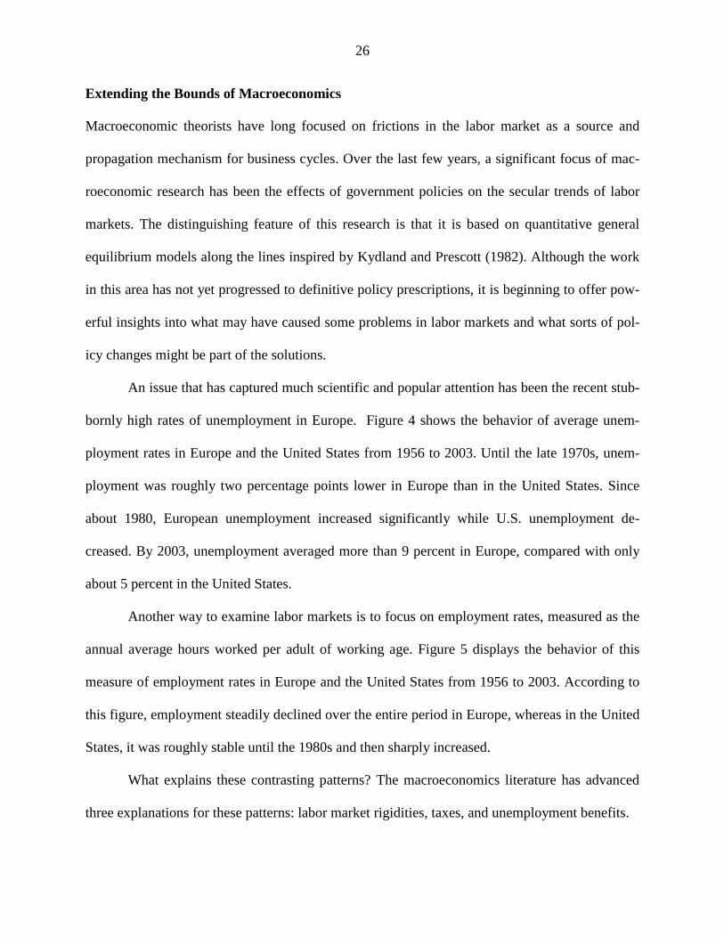
An issue that has captured much scientific and popular attention has been the recent stub-

bornly high rates of unemployment in Europe. Figure 4 shows the behavior of average unem-

ployment rates in Europe and the United States from 1956 to 2003. Until the late 1970s, unem-

ployment was roughly two percentage points lower in Europe than in the United States. Since

about 1980, European unemployment increased significantly while U.S. unemployment de-

creased. By 2003, unemployment averaged more than 9 percent in Europe, compared with only

about 5 percent in the United States.

Another way to examine labor markets is to focus on employment rates, measured as the

annual average hours worked per adult of working age. Figure 5 displays the behavior of this

measure of employment rates in Europe and the United States from 1956 to 2003. According to

this figure, employment steadily declined over the entire period in Europe, whereas in the United

States, it was roughly stable until the 1980s and then sharply increased.

What explains these contrasting patterns? The macroeconomics literature has advanced

three explanations for these patterns: labor market rigidities, taxes, and unemployment benefits.

27

Labor Market Rigidities

One widely held view is that labor markets are much more rigid in Europe than in the

United States. For example, European legal employment protections that make it difficult to fire

workers are typically more stringent than those in the United States. Hopenhayn and Rogerson’s

(1993) general equilibrium model points to two opposing forces of firing costs on unemploy-

ment: the costs make firms more reluctant to fire workers, thereby reducing unemployment; but

at the same time they make firms more reluctant to hire workers in the first place, thereby raising

unemployment. The overall effect is ambiguous and depends on the details of the microeconomic

shocks affecting individual firms’ employment decisions. Using cross-country evidence, Nickell

(1997) finds that the effect of hiring costs is also ambiguous.

Although the effect of firing costs on unemployment is ambiguous, the effect on produc-

tivity in the Hopenhayn and Rogerson (1993) model is not. Firing costs tend to inhibit the effi-

cient reallocation of labor to more productive firms and thereby reduce aggregate productivity.

Thus, this model implies that welfare can be raised by reducing firing costs. Note that if workers

cannot borrow against future earnings to invest in general human capital, then firing costs may

provide incentives for firms to invest in such capital and thus raise productivity, as in the models

of Acemoglu and Pischke (1999) and Chari, Restuccia, and Urrutia (2005).

Taxes

Prescott (2002) and Rogerson (2005) have pointed to differences in taxes as a key source

of the differences in European and U.S. labor market experiences. To study this possibility, the

discipline of general equilibrium theory is essential, because the effect of taxes on labor market

outcomes depends not only on how tax revenue is raised but also, as Rogerson (2005) empha-

sizes, on how it is used. A tax has both a substitution effect that reduces the incentive to work

28

and an income effect that increases the incentive to work, but the way in which tax revenue is

spent can alter the income effects.

To see why the details of how tax revenues are spent are important, suppose first that the

revenue is used to provide public goods that are poor substitutes for private consumption. Then,

as long as the utility function has near unit elasticity of substitution between consumption and

leisure, the income and substitution effects nearly cancel so that labor supply effects of taxes are

approximately zero. Hence, to a first approximation, the public good expenditures crowd out pri-

vate consumption dollar for dollar. Suppose next that the revenue is either transferred back to

private citizens in a lump-sum fashion or, equivalently, used to purchase private goods for citi-

zens. Then taxes have only a substitution effect—because the expenditures offset the income ef-

fect—and labor supply falls.

Prescott (2002) cleverly sidestepped these issues by noting that in a general equilibrium

model, the details of the expenditures are captured by their effects on consumption. Prescott be-

gan his analysis by noting that in a general equilibrium model with a stand-in household, the

first-order condition determining labor supply equates the marginal rate of substitution between

consumption and leisure to the after-tax marginal product of labor. Given consumption and the

capital stock, this condition thus implies a relation between employment and the tax-induced la-

bor wedge. In this approach, the details of how government revenues are spent play a role in de-

termining labor supply only through its effects on consumption and the capital stock.

Assuming that both the utility function and the production function have unit elasticity of

substitution, and using long-term averages to pin down share parameters, Prescott showed that

this simple theory works surprisingly well in accounting for employment observations for the G-

7 countries for the 1970s and the 1990s. With these functional form assumptions, the marginal

29

rate of substitution is proportional to /(1 )c l− , where c denotes consumption and l the fraction of

time in market work, whereas the after-tax marginal product of labor is proportional to

(1 ) / ,y l− τ so that the consumption-to-output ratio, / ,c y summarizes the effects of the details of

expenditures as well as other aspects of the model, such as capital income taxes. Table 2 is re-

produced from Prescott (2002). The closeness between the predictions of his simple model and

the data is remarkable.

The Prescott analysis works well in a comparison of the early 1970s and the mid-1990s,

in part because tax policies clearly changed dramatically during this time. Using his analysis to

compare the 1950s and the 1970s, however, does not work as well. Evidence of large changes in

tax rates from the 1950s to the 1970s is hard to find, even though Figure 5 shows a sustained de-

cline in employment rates over this period. As Prescott has acknowledged, his analysis likewise

does not work well for the Scandinavian countries that have both high tax rates and high em-

ployment.

Rogerson (2005) has built on Prescott’s analysis to allow for secular shifts from agricul-

ture and industry toward services. Rogerson argued that changes in taxes and in industry compo-

sition can account for the bulk of observed differences in employment between Europe and the

United States.

These analyses focus on the division of time between market work and all forms of non-

market activities—including both unemployment and being out of the labor force. As such, these

analyses have sharp implications for the behavior of the employment rate. Since they do not dis-

tinguish between search activities and other nonmarket activities that lead households to be clas-

sified as out of the labor force, they are silent about differences in unemployment rates between

Europe and the United States.

30

Unemployment Benefits

One possible reason for why the unemployment rate is higher in Europe than in the

United States is that unemployment benefits are more generous in Europe. A reasonable conjec-

ture is that this greater generosity leads to higher unemployment rates by making workers more

reluctant to accept job offers. The problem with this conjecture is that it seems contradicted by

facts; in the 1960s and 1970s, unemployment benefits were much more generous in Europe than

in the United States, while unemployment rates were lower in Europe than in the United States.

Ljungqvist and Sargent (1998) developed a model that focuses on the division of time between

market work and the search activities of unemployed workers while abstracting from considera-

tions of nonmarket activities other than search. They showed that in the 1960s and 1970s, more

generous unemployment benefits, together with higher firing costs, led Europe to have lower un-

employment rates than in the United States, whereas in the 1980s, the same benefits and firing

costs led to the opposite relationship.

The key difference between the earlier and later periods is that microeconomic turbu-

lence, measured as fluctuations in individual worker productivities, has increased over time in

both Europe and the United States (see Gottschalk and Moffitt, 1994). As microeconomic turbu-

lence increases, more workers find themselves in low-productivity jobs as well as in unemploy-

ment. If unemployment benefits are generous, as they are in Europe, then unemployed workers’

reservation wages fall by only a small amount as turbulence increases, and the flow of workers

out of unemployment does not change much. Hence, with increased microeconomic turbulence,

the overall unemployment rate rises. If unemployment benefits are meager, as they are in the

United States, then workers’ reservation wages fall sharply as turbulence increases, and the out-

31

flow from unemployment rises nearly one-for-one with the inflow. Hence, the unemployment

rate does not change much.

The Ljungqvist and Sargent (1998) model assumes that workers are risk-neutral, in which

case unemployment compensation has no benefits and is costly because it distorts the search de-

cision. As the model stands, the policy implication is that government-provided unemployment

benefits should be eliminated. With risk aversion and imperfections in private markets for unem-

ployment insurance, unemployment insurance has benefits that need to be weighed against the

induced distortions in search decisions. A growing literature has begun to analyze these trade-

offs (for example, Atkeson and Lucas, 1992; Hopenhayn and Nicolini, 1997; Shimer and Wern-

ing, 2005).

In our view, explanations of patterns in European and American labor markets based on

labor market rigidities, taxes, and unemployment benefits all have plausible appeal, but the quan-

titative importance of each has not been definitively established.

Conclusion

Here we have argued that macroeconomic theory has had a profound and far-reaching effect on

the institutions and practices governing monetary policy and is beginning to have a similar effect

on fiscal policy. The marginal social product of macroeconomic science is surely large and

growing rapidly.

Those economists caught up in the frenzy of day-to-day policymaking often view their

colleagues who toil in the ivory towers of academe as having no power to affect practical policy

and those economists who whisper in the ears of presidents and Congress members as having the

ability to dramatically affect policy. The truth, as we have argued, is very far from this view. The

course of practical policy is affected primarily by the institutions we devise and how well presi-

32

dents and Congress members understand economic trade-offs. The day-to-day economic adviser

is useful to the extent that the adviser can educate policymakers about trade-offs, but is largely

irrelevant otherwise. It is easy to see why those economists caught up in the whirlwind of day-

to-day policymaking miss the dramatic changes in policy that result from slow, secular changes

in institutions, practices, and mind-sets.

The toilers in academe are uniquely placed to develop analyses of institutions and to edu-

cate the public and policymakers about economic trade-offs. The essence of our argument is that,

at least in macroeconomics, these toilers have delivered large returns to society over the last sev-

eral decades.

33

Notes 1The use of dynamic general equilibrium models in macroeconomics has a long tradition

dating back, at least, to Robert Solow (1956).

2Note that these practical concerns are consistent with the work of Sargent and Wallace

(1985), who emphasized that monetary and fiscal policy are linked by a single government

budget constraint, so that responsible monetary policy is impossible without responsible fiscal

policy.

3With a production function of the form 1 ,y Ak lα −α= it is straightforward to show that

1

log log log .1 1

y kA

l y

α⎛ ⎞ = +⎜ ⎟ − α − α⎝ ⎠

Using the assumption that A is the same across countries, removing means, and setting α = 2/3

gives the relationship described in the text.

34

References

Acemoglu, Daron and Jörn-Steffen Pischke. 1999. “The Structure of Wages and In-

vestment in General Training.” Journal of Political Economy. June, 107:3, pp. 539–72.

Aiyagari, S. Rao, Albert Marcet, Thomas J. Sargent and Juha Seppälä. 2002. “Op-

timal Taxation without State-Contingent Debt.” Journal of Political Economy. December, 110:6,

pp. 1220–4.

Alesina, Alberto and Lawrence H. Summers. 1993. “Central Bank Independence and

Macroeconomic Performance: Some Comparative Evidence.” Journal of Money, Credit, and

Banking. May, 25:2, pp. 151–62.

Angeletos, George-Marios. 2002. “Fiscal Policy with Noncontingent Debt and the Op-

timal Maturity Structure.” Quarterly Journal of Economics. August, 117:3, pp. 1105–31.

Athey, Susan, Andrew Atkeson, and Patrick J. Kehoe. 2005. “The Optimal Degree of

Discretion in Monetary Policy.” Econometrica. September, 73:5, pp. 1431–75.

Atkeson, Andrew and Robert E. Lucas Jr. 1992. “On Efficient Distribution with Pri-

vate Information.” Review of Economic Studies. July, 59:200, pp. 427–53.

Barro, Robert J. 1979. “On the Determination of the Public Debt.” Journal of Political

Economy. October, 87:5, pp. 940–71.

Barro, Robert J. and David Gordon. 1983. “Rules, Discretion and Reputation in a

Model of Monetary Policy.” Journal of Monetary Economics. July, 1983, 12:1, pp. 101–21.

Benigno, Pierpaolo and Michael Woodford. 2003. “Optimal Monetary and Fiscal Pol-

icy: A Linear-Quadratic Approach.” National Bureau of Economic Research Working Paper No.

9905, August.

35

Bernanke, Ben S., Thomas Laubach, Frederic S. Mishkin and Adam S. Posen. 1999.

Inflation Targeting: Lessons from the International Experience. Princeton, N.J.: Princeton Uni-

versity Press.

Bernanke, Ben S. and Frederic S. Mishkin. 1997. “Inflation Targeting: A New Frame-

work for Monetary Policy?” Journal of Economic Perspectives. Spring, 11:2, pp. 97–116.

Calvo, Guillermo A. 1978. “On the Time Consistency of Optimal Policy in a Monetary

Economy.” Econometrica. November, 46:6, pp. 1411–28.

Chari, V. V., Lawrence J. Christiano and Patrick J. Kehoe. 1991. “Optimal Fiscal

and Monetary Policy: Some Recent Results.” Journal of Money, Credit, and Banking. August,

23:3, pp. 519–39.

Chari, V. V., Lawrence J. Christiano and Patrick J. Kehoe. 1994. “Optimal Fiscal

Policy in a Business Cycle Model.” Journal of Political Economy. August, 102:4, pp. 617–52.

Chari, V. V., Lawrence J. Christiano and Patrick J. Kehoe. 1996. “Optimality of the

Friedman Rule in Economies with Distorting Taxes.” Journal of Monetary Economics. April,

37:2, pp. 203–23.

Chari, V. V., Patrick J. Kehoe and Ellen McGrattan. 1997. “The Poverty of Nations:

A Quantitative Investigation.” Research Department Staff Report 204, Federal Reserve Bank of

Minneapolis.

Chari, V. V., Patrick J. Kehoe and Edward C. Prescott. 1989. “Time Consistency and

Policy.” In Modern Business Cycle Theory, edited by Robert Barro, 265-305, Cambridge, Mass.:

Harvard University Press.

Chari, V. V., Diego Restuccia and Carlos Urrutia. 2005. “On-the-Job Training, Lim-

ited Commitment, and Firing Costs.” Working Paper, Federal Reserve Bank of Minneapolis.

36

Cooley, Thomas, F. 1995. Frontiers of Business Cycle Research. Princeton, N.J.: Prince-

ton University Press.

Correia, Isabel, Juan Pablo Nicolini and Pedro Teles. 2004. “Optimal Fiscal and

Monetary Policy: Equivalence Results.” Working Paper, Bank of Portugal.

da Costa, Carlos and Iván Werning. 2003. “On the Optimality of the Friedman Rule

with Heterogeneous Agents and Non-Linear Income Taxation.” Mimeo, University of Chicago.

Fischer, Stanley. 1980. “Dynamic Inconsistency, Cooperation, and the Benevolent, Dis-

sembling Government.” Journal of Economic Dynamics and Control. February, 2:1, pp. 93–107.

Friedman, Milton. 1969. “The Optimum Quantity of Money.” In The Optimum Quantity

of Money and Other Essays. Chicago: Aldine, pp. 1–50.

Gottschalk, Peter and Robert Moffitt. 1994. “The Growth of Earnings Instability in the

U.S. Labor Market.” Brookings Papers on Economic Activity. 1994:2, 217–72.

Gravelle, Jane G. 2004. “Historical Effective Marginal Tax Rates on Capital Income.”

Congressional Research Service Report for Congress. January 12.

Hopenhayn, Hugo A. and Juan Pablo Nicolini. 1997. “Optimal Unemployment Insur-

ance.” Journal of Political Economy. April, 105:2, pp. 412–38.

Hopenhayn, Hugo and Richard Rogerson. 1993. “Job Turnover and Policy Evaluation:

A General Equilibrium Analysis.” Journal of Political Economy. October, 101:5, pp. 915–38.

Khan, Aubhik, Robert G. King and Alexander L. Wolman. 2003. “Optimal Monetary

Policy.” Review of Economic Studies. October, 70:247, pp. 825–60.

Kydland, Finn E. and Edward C. Prescott. 1977. “Rules Rather than Discretion: The

Inconsistency of Optimal Plans.” Journal of Political Economy. June, 85:3, pp. 473–91.

37

Kydland, Finn E. and Edward C. Prescott. 1982. “Time to Build and Aggregate Fluc-

tuations.” Econometrica. November, 50:6, pp. 1345–70.

Levine, David K. 1991. “Asset Trading Mechanisms and Expansionary Policy.” Journal

of Economic Theory. June, 54:1, pp. 148–64.

Ljungqvist, Lars and Thomas J. Sargent. 1998. “The European Unemployment Di-

lemma.” Journal of Political Economy. June, 106:3, pp. 514–50.

Lucas, Robert E., Jr. 1976. “Econometric Policy Evaluation: A Critique.” Journal of

Monetary Economics. Supplementary Series, 1:2, pp. 19–46.

Lucas, Robert E., Jr. 1986. “Principles of Fiscal and Monetary Policy.” Journal of

Monetary Economics. July, 17:1, pp. 117–34.

Lucas, Robert E., Jr. and Nancy L. Stokey. 1983. “Optimal Fiscal and Monetary Pol-

icy in an Economy without Capital.” Journal of Monetary Economics. July, 12:1, pp. 55–93.

Mankiw, N. Gregory, David Romer and David N. Weil. 1992. “A Contribution to the

Empirics of Economic Growth.” Quarterly Journal of Economics. May, 107:2, pp. 407–37.

Nicholl, Peter W. E. and David J. Archer. 1992. “An Announced Downward Path for

Inflation.” Reserve Bank Bulletin. 55:4, pp. 315–23. New Zealand Reserve Bank.

Nickell, Stephen. 1997. “Unemployment and Labor Market Rigidities: Europe versus

North America.” Journal of Economic Perspectives. Summer, 11:3, pp. 55–74.

Phelps, Edmund. 1973. “Inflation in the Theory of Public Finance.” Swedish Journal of

Economics. March, 75, pp. 67–82.

Prescott, Edward C. 2002. “Richard T. Ely Lecture: Prosperity and Depression.” Ameri-

can Economic Review. May, 92:2, pp. 1–15.

38

Ramsey, Frank P. 1927. “A Contribution to the Theory of Taxation.” Economic Jour-

nal. March, 37:145, pp. 47–61.

“Report of the President’s Advisory Panel on Federal Tax Reform.” November 2005.

Washington, D.C.: Government Printing Office.

Rogerson, Richard. 2005. “Structural Transformation and the Deterioration of European

Labor Market Outcomes.” Mimeo, Arizona State University.

Rogoff, Kenneth. 1985. “The Optimal Degree of Commitment to an Intermediate Mone-

tary Target.” Quarterly Journal of Economics. November, 100:4, pp. 1169–89.

Sargent, Thomas J. and Neil Wallace. 1985. “Some Unpleasant Monetarist Arithme-

tic.” Federal Reserve Bank of Minneapolis Quarterly Review. Winter, 9:1, pp. 15–31.

Schmitt-Grohé, Stephanie and Martín Uribe. 2004. “Optimal Fiscal and Monetary

Policy under Sticky Prices.” Journal of Economic Theory. February, 114:2, pp. 198–230.

Shimer, Robert and Iván Werning. 2005. “Liquidity and Insurance for the Unem-

ployed.” National Bureau of Economic Research Working Paper No. 11689.

Siu, Henry E. 2004. “Optimal Fiscal and Monetary Policy with Sticky Prices.” Journal

of Monetary Economics. April, 51:3, pp. 575–607.

Solow, Robert, M. 1956. “A Contribution to the Theory of Economic Growth.” Quar-

terly Journal of Economics. 70:1, pp. 65–94.

Strotz, Robert H. 1955. “Myopia and Inconsistency in Dynamic Utility Maximization.”

Review of Economic Studies. 23:3, pp. 165–80.

Taylor, John B. 1993. “Discretion versus Policy Rules in Practice.” Carnegie-Rochester

Conference Series on Public Policy. December, 39, pp. 195–214.

39

Truman, Edwin M. 2003. Inflation Targeting in the World Economy. Washington, D.C.:

Institute for International Economics.

Weichenrieder, Alfons J. 2005. “(Why) Do We Need Corporate Taxation?” CESifo

Working Paper No. 1495, July. Institute for Economic Research, Munich, Germany.

Werning, Iván. 2005. “Tax Smoothing with Redistribution.” Working paper, Massachu-

setts Institute of Technology.

Table 1

Effective U.S. Marginal Tax Rates

on Capital Income, 1953–2003

Time Period % 1953–59 47.3 1960s 35.8 1970s 41.3 1980s 35.3 1990s 30.5 2000–03 28.3

Source: Gravelle (2004)

Table 2

G-7 Countries’ Predicted and Actual Labor Supply Employment*

Labor Supply in 1970–74 Country

Tax rate τ

Consumption-Output Ratio

c/y

Actual

Predicted Germany .52 .66 24.6 24.6

France .49 .66 24.4 25.4

Italy .41 .66 19.2 28.3

Canada .44 .72 22.2 25.6

United Kingdom .45 .77 25.9 24.0

Japan .25 .60 29.8 35.8

United States .40 .74 23.5 26.4

Source: Prescott (2002) *Hours worked per week per person aged 15–64

Figure 1Central Bank Independence vs. Inflation

Measures of Central Bank Independence vs. Average Rates of Inflation in 16 Countries, 1973–88

BEL

NZ

SPA

ITA

UKDEN

FRA/NOR/SWEAUS

JAP

NETCAN

US

SWIGER

2

3

4

5

6

7

8

9

0.5 1 1.5 2 2.5 3 3.5 4 4.5

Index of Central Bank Independence

Ave

rage

Infla

tion

Rat

e (%

)

Source: Alesina and Summers (1993)

Figure 2a United Kingdom

0

2

4

6

8

10

12

1980 1981 1982 1983 1984 1985 1986 1987 1988 1989 1990 1991 1992 1993 1994 1995 1996 1997

Inflation Targeting RegimeDiscretionary Regime

Source: Bernanke et al. (1999)

Figures 2Examples of Inflation in Discretionary and Targeting Regimes, 1980–98

InflationRate(%)

Bands for the Targets

Figure 2bNew Zealand

0

2

4

6

8

10

12

14

16

18

20

1980 1982 1984 1986 1988 1990 1992 1994 1996

Bands for the Targets

Inflation Targeting RegimeDiscretionary Regime

Source: Bernanke et al. (1999)

Figure 2cCanada

-2

0

2

4

6

8

10

12

14

1980 1981 1982 1983 1984 1985 1986 1987 1988 1989 1990 1991 1992 1993 1994 1995 1996 1997

Bands for the Targets

Inflation Targeting RegimeDiscretionary Regime

Source: Bernanke et al. (1999)

Figure 2d Inflation in Discretionary and Targeting Regimes—Sweden

-6

-2

2

6

10

14

18

1980 1981 1982 1983 1984 1985 1986 1987 1988 1989 1990 1991 1992 1993 1994 1995 1996 1997

Bands for the Targets

Inflation Targeting RegimeDiscretionary Regime

Source: Bernanke et al. (1999)

-4

-2

0

2

4

-4 -2 0 2 4

log(

Y/ L

) (re

lativ

e to

its

mea

n)

Source: Chari, Kehoe, and McGrattan (1997)

2 log (k /y ) (relative to its mean)

Figure 3The Relationship Between Capital-Output Ratios and Relative Income Levels

in 125 Countries During the Period 1950–85

RelativeOutput Ratio

Capital-Output Ratio

Figure 3 Note: If countries i = 1, . . . , I have an aggregate production function for aggregate output of the form 2/3 1/3 i i iY AK L= with common productivity parameter A and country-specific (broadly

measured) capital Ki and labor Li, then relative to their respective means, log ( / )i iK L −

2 log( / ).i iK Y

2

3

4

5

6

7

8

9

10

11

1956 1961 1966 1971 1976 1981 1986 1991 1996 2001

Figure 4Unemployment Rates

Source: Rogerson (2005)

Europe

United States

Unemploymentas % ofLabor Force

Figures 4–5Unemployment and Employment in Europe and the United States, 1956–2003

900

950

1000

1050

1100

1150

1200

1250

1300

1350

1400

1956 1961 1966 1971 1976 1981 1986 1991 1996 2001

Figure 5Average Annual Hours Worked

Source: Rogerson (2005)

United States

Europe

Hours