Embed Size (px)
Citation preview

Modern Space/Time Geostatistics Using River Distances: Theory and Applications for Water Quality Mapping
Eric S. Money
A dissertation submitted to the faculty of the University of North Carolina at Chapel Hill in partial fulfillment of the requirements for the degree of Doctor of Philosophy in
the Department of Environmental Sciences and Engineering.
Chapel Hill 2008
Approved by:
Marc L. Serre
Gregory W. Characklis
Kenneth H. Reckhow
Martin W. Doyle
Lawrence E. Band
D. Derek Aday

ii
© 2009 Eric S. Money
ALL RIGHTS RESERVED

iii
Abstract Eric S. Money
Modern Space/Time Geostatistics Using River Distances: Theory and Applications for Water Quality Mapping
(Under the direction of Dr. Marc L. Serre)
The Clean Water Act requires that state and local agencies assess all river
miles for potential impairments. However, due to the large number of river miles to
be assessed, as well as budget and resource limitations, many states cannot
feasibly meet this requirement. Therefore, there is a need for a framework that can
accurately assess water quality at un-monitored locations, using limited data
resources. Many researchers employ geostatistical techniques such as kriging and
Bayesian Maximum Entropy (BME) to interpolate values in areas where no data
exist. These techniques rely on the spatial and/or temporal autocorrelation between
existing data points to estimate at un-monitored locations. This autocorrelation is
traditionally a function of the Euclidean distance between those data points;
however, a Euclidean distance does not take into account that many water quality
variables may be spatially correlated due to the hydrogeography of the system.
The focus of this work is the development of a space/time geostatistical
framework for estimating and mapping water quality along river networks by using
river distances instead of the traditional Euclidean distance. The Bayesian
Maximum Entropy method of modern space/time geostatistics is modified and
extended to incorporate the use of river distances to improve the estimation of basin-
wide water quality. This new framework, termed river-BME, uses geostatistical

iv
models that integrate the use of permissible covariance functions with secondary
information along with river distance. Factors, such as network complexity, are
explored to determine the efficacy of using river-BME for water quality estimation.
Additionally, simulation experiments and three real world case studies provide a
broad application of this framework for a variety of basins and water quality
parameters, including dissolved oxygen, Escherichia coli, and fish tissue mercury.
Results show that the use of river-BME produces significantly more accurate
estimates of water quality at un-monitored locations than traditional Euclidean based
methods by more than 30%. Overall, this work provides a new tool for applying
modern space/time geostatistics using river distances. It has the potential to aid not
only future researchers but can ultimately provide environmental managers with the
information necessary to better allocate resources and protect ecological and human
health.

v
Acknowledgements
First and foremost I would like to thank my advisor, Marc Serre, for his
support, guidance, and mentorship during my tenure as a PhD student. Marc
provided me with the encouragement and skills necessary to succeed in this
sometimes long and arduous process. I will be forever grateful for his mentorship
and friendship.
I would also like to thank the members of my committee for providing great
insight and suggestions that have enhanced this body of work.
I am also grateful to the New Jersey Department of Environmental Protection
and the North Carolina Water Resources Research Institute for funding many
important aspects of this work. Without their support, much of this research may not
have been possible. I particularly would like to think Gail Carter for providing a great
deal of support to the projects with the state of New Jersey.
Last, but not least, I would like to thank my family and friends for their
encouragement and unyielding support throughout this process. Without them the
task of completing a PhD would have seemed much more daunting. I am privileged
to have had so many people support me during this process and I thank each and
every one of them.

vi
Table of Contents
List of Tables ............................................................................................................. xi List of Figures ........................................................................................................... xii Chapter
I. Introduction ................................................................................................. 1 II. Modern Space/Time Geostatistics Using River Distances: The Conceptual Framework ............................................................................... 6 2.1. Introduction .......................................................................................... 6 2.2. The Bayesian Maximum Entropy Framework ....................................... 6 2.2.1. The Stages of BME ................................................................... 7 2.2.2. The General Knowledge Base ................................................... 9 2.2.3. The Site-Specific Knowledge Base ......................................... 10 2.2.4. Bayesian Conditionalization .................................................... 12 2.3. Distance Metrics ................................................................................. 13 2.4. Covariance Models Using River Distances ........................................ 15 2.4.1. Isotropic River Covariance Models .......................................... 15 2.4.2. Flow-Weighted River Covariance Models ............................... 20 2.4.3. River Covariance Model Selection .......................................... 21 2.5. River Estimation and Mapping ........................................................... 23 2.5.1. Estimation Neighborhood Selection ........................................ 23

vii
2.5.2. Mapping River Estimates ........................................................ 25 2.6. Summary ........................................................................................... 26 III. Modern Space/Time Geostatistics Using River Distances: Numerical Implementation ......................................................................................... 27 3.1. Introduction ....................................................................................... 27 3.2. The River Algorithm ........................................................................... 27 3.3. The river-BME Framework ................................................................ 30 3.3.1. Development of New River Based Functions .......................... 30 3.3.2. Modification of Existing BME Functions .................................. 35 3.4. Efficacy of river-BME ......................................................................... 36 3.4.1. Parameter Choice ................................................................... 36 3.4.2. Data Density ............................................................................ 38 3.4.3. Measures of Network Complexity ............................................ 39 3.4.3.1. Branching Level .......................................................... 40 3.4.3.2. Meandering Ratio ....................................................... 43 3.5. Using river-BME in Simulated Case Studies .................................... 45 3.5.1. Case Study Using Data Simulated on a Synthetic Stream Reach ..................................................................................... 45 3.5.2. Cast Study Using Data Simulated on a Real River Network .. 48 IV. Modern Space/Time Geostatistics Using River Distances: A Case Study of Dissolved Oxygen ...................................................................... 51 4.1. Introduction ...................................................................................... 51 4.2. Materials and Methods .................................................................... 53 4.2.1. Study Area ............................................................................. 53 4.2.2. Dissolved Oxygen Data ......................................................... 55

viii
4.2.3. Space/Time Covariance Modeling Using River Distance ...... 56 4.2.4. Estimation of Dissolved Oxygen ............................................ 57 4.2.5. Assessment of Impaired River Miles ..................................... 59 4.3. Results and Discussion ................................................................... 60 4.3.1. Covariance of DO in New Jersey .......................................... 60 4.3.2. Euclidean vs. River Estimation .............................................. 63 4.3.3. River-BME Estimation of DO ................................................. 67 4.3.4. Impaired River Miles in the Raritan and Lower Delaware Basins ................................................................................... 68 V. Modern Space/Time Geostatistics Using River Distances: A Case Study of Turbidity and Escherichia coli .................................................... 72 5.1. Introduction ...................................................................................... 72 5.1.1. Fecal Indicator Bacteria in River Systems .............................. 72 5.1.2. Autocorrelation in E.coli .......................................................... 74 5.1.3. Turbidity and E.coli ................................................................. 75 5.2. Materials and Methods ..................................................................... 75 5.2.1. Data and Study Area .............................................................. 75 5.2.2. Generation of Soft Data .......................................................... 77 5.2.3. Integrating Hard and Soft Data ............................................... 78 5.2.4. Space/Time Covariance Modeling Using River Distance ....... 79 5.2.5. Comparing Euclidean and River Estimation ........................... 79 5.2.6. Estimation of E.coli ................................................................. 80 5.2.7. Assessment of Impaired River Miles ...................................... 81 5.3. Results and Discussion .................................................................... 82

ix
5.3.1. Covariance Analysis ............................................................... 82 5.3.2. Cross-validation Analysis ....................................................... 84 5.3.3. Assessment of Fecal Contamination in the Raritan Basin ...... 85 VI. Modern Space/Time Geostatistics Using River Distances: A Case Study of Fish Tissue Mercury ................................................................... 89 6.1. Introduction ...................................................................................... 89 6.1.1. Mercury in the Environment .................................................... 89 6.1.2. Autocorrelation of Fish Tissue Mercury .................................. 91 6.1.3. Factors Influencing the Bioaccumulation of Mercury .............. 92 6.2. Materials and Methods ..................................................................... 93 6.2.1. Data and Study Area .............................................................. 93 6.2.2. Generation of Soft Data from Multiple Sources ...................... 95 6.2.3. Integrating Hard and Soft Data ............................................... 97 6.2.4. Space/Time Covariance Models that Use River Distances .... 98 6.2.5. Comparing Euclidean and River Estimations ......................... 99 6.2.6. Estimation of Fish Tissue Hg ................................................ 100 6.2.7. Assessment of Impaired River Miles .................................... 100 6.3. Results and Discussion .................................................................. 101 6.3.1. Covariance Analysis ............................................................. 101 6.3.2. Cross-validation Analysis ..................................................... 103 6.3.3. Assessment of Fish Tissue Mercury ..................................... 105 VII. Concluding Remarks............................................................................. 110
Appendices ............................................................................................................ 114

x
Appendix A: Proof of Permissibility for Exponential Covariance Models Using River Distance ............................................................. 114 Appendix B: Mathematical Summary of Flow-weighted Covariance Models .................................................................................. 117 Appendix C: Flow-additive Functions ......................................................... 122 Appendix D: Movies Depicting Water Quality Trends Using river-BME ..... 126 Works Cited ........................................................................................................... 128

xi
List of Tables Table
3.1. Summary of new and modified functions integrated into the river-BME Framework ............................................................................................... 36 4.1. Water quality estimation studies using river covariance models .............. 52 4.2. Basic Statistics for monitored DO data (raw-mg/L) for the period January, 1990 – August, 2005 for the Raritan and Lower Delaware River basins in New Jersey ..................................................................... 56 4.3. Space/time covariance parameters for DO using a river metric ............... 61 4.4. Change in cross validation mean square error (MSE) for each basin. A negative change indicates a reduction in overall MSE (i.e. improvement) when using a river metric ........................................... 64 4.5. Seasonal Average Variation in Fraction (%) of River Miles More Likely than Not (MLTN) in Non-Attainment (probability of Violation > 50%) for 2002 .................................................. 69 4.6. Summer Fraction (%) of River Miles More Likely than Not (MLTN) in Non- Attainment (probability of Violation > 50%) for the period 2000-2005 (Summer = Jul- Sep) ............................................................. 69 5.1. E.coli space/time covariance model parameters ..................................... 83 6.1. Data summary for mercury and pH in the Cape Fear and Lumber Basins, 1990-2004 ................................................................................... 95 6.2. Cross-validation scenarios for fish tissue Hg estimates using river-BME and Euclidean-BME ................................................................ 99 6.3. FishHg space/time covariance model parameters ................................. 102 7.1. Summary of river-BME estimation studies ............................................. 111
xii
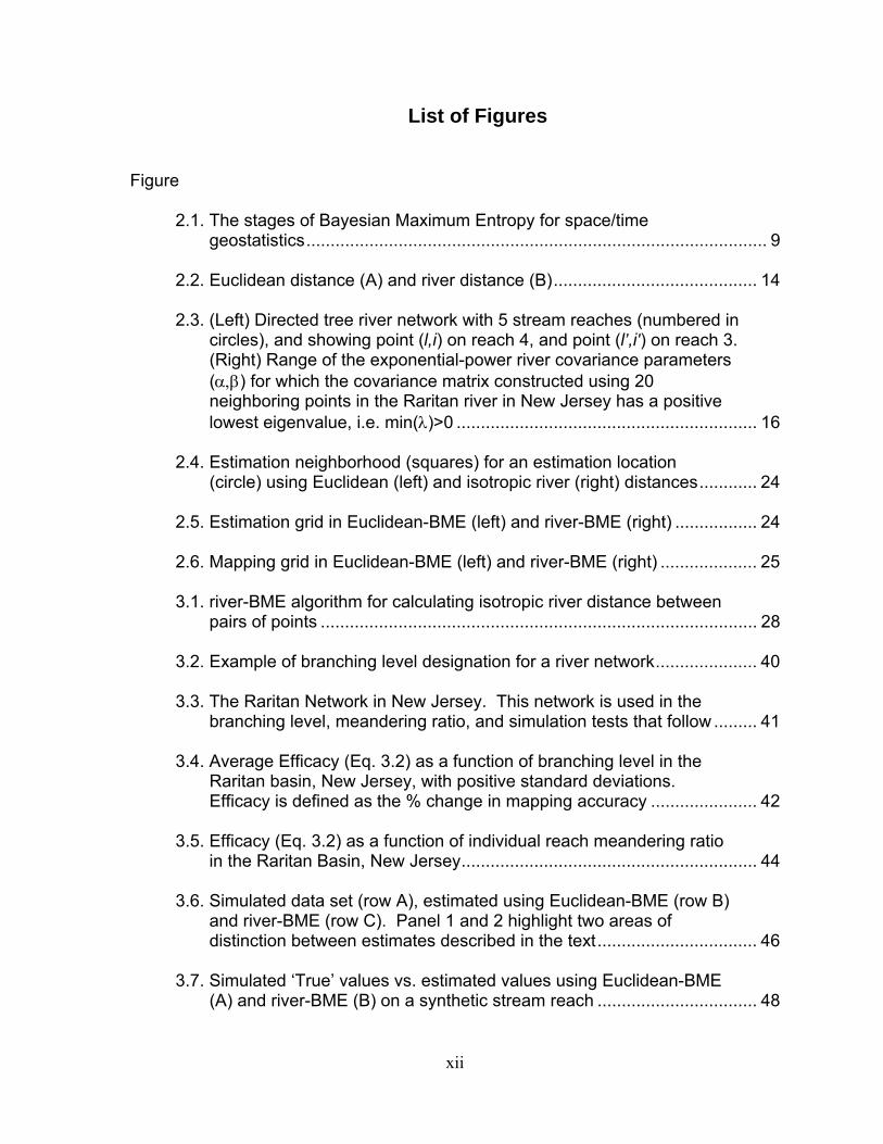
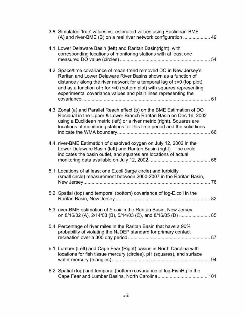
List of Figures
Figure
2.1. The stages of Bayesian Maximum Entropy for space/time geostatistics ............................................................................................... 9 2.2. Euclidean distance (A) and river distance (B) .......................................... 14 2.3. (Left) Directed tree river network with 5 stream reaches (numbered in circles), and showing point (l,i) on reach 4, and point (l’,i') on reach 3. (Right) Range of the exponential-power river covariance parameters () for which the covariance matrix constructed using 20 neighboring points in the Raritan river in New Jersey has a positive lowest eigenvalue, i.e. min()>0 .............................................................. 16 2.4. Estimation neighborhood (squares) for an estimation location (circle) using Euclidean (left) and isotropic river (right) distances ............ 24 2.5. Estimation grid in Euclidean-BME (left) and river-BME (right) ................. 24 2.6. Mapping grid in Euclidean-BME (left) and river-BME (right) .................... 25 3.1. river-BME algorithm for calculating isotropic river distance between pairs of points .......................................................................................... 28 3.2. Example of branching level designation for a river network ..................... 40 3.3. The Raritan Network in New Jersey. This network is used in the branching level, meandering ratio, and simulation tests that follow ......... 41 3.4. Average Efficacy (Eq. 3.2) as a function of branching level in the Raritan basin, New Jersey, with positive standard deviations. Efficacy is defined as the % change in mapping accuracy ...................... 42 3.5. Efficacy (Eq. 3.2) as a function of individual reach meandering ratio in the Raritan Basin, New Jersey ............................................................. 44 3.6. Simulated data set (row A), estimated using Euclidean-BME (row B) and river-BME (row C). Panel 1 and 2 highlight two areas of distinction between estimates described in the text ................................. 46 3.7. Simulated ‘True’ values vs. estimated values using Euclidean-BME (A) and river-BME (B) on a synthetic stream reach ................................. 48
xiii
3.8. Simulated ‘true’ values vs. estimated values using Euclidean-BME (A) and river-BME (B) on a real river network configuration .................... 49 4.1. Lower Delaware Basin (left) and Raritan Basin(right), with corresponding locations of monitoring stations with at least one measured DO value (circles) ................................................................... 54 4.2. Space/time covariance of mean-trend removed DO in New Jersey’s Raritan and Lower Delaware River Basins shown as a function of distance r along the river network for a temporal lag of =0 (top plot) and as a function of for r=0 (bottom plot) with squares representing experimental covariance values and plain lines representing the covariance ............................................................................................... 61 4.3. Zonal (a) and Parallel Reach effect (b) on the BME Estimation of DO Residual in the Upper & Lower Branch Raritan Basin on Dec 16, 2002 using a Euclidean metric (left) or a river metric (right). Squares are locations of monitoring stations for this time period and the solid lines indicate the WMA boundary ..................................................................... 66 4.4. river-BME Estimation of dissolved oxygen on July 12, 2002 in the Lower Delaware Basin (left) and Raritan Basin (right). The circle indicates the basin outlet, and squares are locations of actual monitoring data available on July 12, 2002.............................................. 68 5.1. Locations of at least one E.coli (large circle) and turbidity (small circle) measurement between 2000-2007 in the Raritan Basin, New Jersey .............................................................................................. 76 5.2. Spatial (top) and temporal (bottom) covariance of log-E.coli in the Raritan Basin, New Jersey ...................................................................... 82 5.3. river-BME estimation of E.coli in the Raritan Basin, New Jersey on 8/16/02 (A), 2/14/03 (B), 5/14/03 (C), and 8/16/05 (D) ....................... 85 5.4. Percentage of river miles in the Raritan Basin that have a 90% probability of violating the NJDEP standard for primary contact recreation over a 300 day period ............................................................. 87 6.1. Lumber (Left) and Cape Fear (Right) basins in North Carolina with locations for fish tissue mercury (circles), pH (squares), and surface water mercury (triangles) ......................................................................... 94 6.2. Spatial (top) and temporal (bottom) covariance of log-FishHg in the Cape Fear and Lumber Basins, North Carolina ..................................... 101

xiv
6.3. river-BME Fish Tissue Mercury estimates (ppm) in the Cape Fear and Lumber Basins on July 23, 1995 (A); July 2, 1999 (B); June 26, 2000 (C); and May 13, 2004 (D). Squares indicate locations of actual fish tissue measurements ........................................ 106 6.4. Percentage of river miles with fish tissue mercury median estimate exceeding Mercury Action Levels set by the FDA (top; 1.0ppm), North Carolina (middle; 0.4ppm), and the EPA (bottom; 0.3ppm) ................... 107 C.1. Example of a river with 5 reaches, indicating for each reach i the contributing watershed area ai within reach i, the total watershed area Ai at the downstream end of reach i, and the corresponding flow additive function (i) ............................................................................. 124

Chapter I: Introduction
The primary focus of this work is the application of river distances to the
geostatistical estimation of water quality along river networks. A substantial portion
of this research consists of the development of a river metric that can be
incorporated into the Bayesian Maximum Entropy methodology for the
spatiotemporal estimation and mapping of water quality. This is the first known
attempt to fully implement a river metric into the spatiotemporal estimation of water
quality for a series of parameters and across multiple basins. The overall hypothesis
is that by accounting for the river connectedness between data points, the
space/time estimation and mapping accuracy of basin-wide water quality can be
improved significantly.
There have been several studies that attempt to characterize surface water
quality using geostatistics. Many of these studies involve traditional kriging
techniques, or other interpolation and regression based methods with a Euclidean
distance (Rasmussen et al., 2005; Tortorelli and Pickup, 2006; Cressie et al., 2005;
Peterson and Urquhart, 2006). Cressie et al. (2005) and Peterson and Urquhart
(2006) consider the use of river distance but ultimately perform estimations using a
Euclidean approach. These studies raise additional questions about the effect of
using a river distance for water quality estimation. Therefore this research extends

2
previous work to compare geostatistical estimation of water quality using river and
Euclidean distances in a space/time framework.
Recent developments in geostatistics have begun to address both the spatial
and temporal variability as well (Stein 1986, Christakos 1992, Cressie 1993, Bogaert
1996, Kyriakidis and Journel 1999, Fuentes 2004, Kolovos et al. 2004, Akita et al.
2007). In the case of many water quality parameters, temporal variability plays a
key role in understanding the overall impact on a basin-wide system.
Spatiotemporal methods aim at rigorously modeling the spatial and temporal
variability inherent in data so as to produce more accurate estimates and
significantly reduce overall estimation error for a variety of environmental parameters
at unmonitored space/time locations using the generally sparse monitoring data
available.
One such method is the spatiotemporal Bayesian Maximum Entropy (BME)
method (Christakos 1990, 2000; Serre et al. 1998, Serre and Christakos, 1999).
This method has been successfully applied to a variety of environmental issues,
including air quality (Christakos and Serre, 2000; Christakos et al. 2004; Wilson and
Serre 2007), and epidemiology (Law et al. 2004, 2006). There have also been
several interesting studies that involve the BME estimation of water quality (Serre et
al. 2004, LoBuglio et al., 2007; Akita et al. 2007, Couillette et al., 2008). These
studies have shown that by using space/time BME we can produce more accurate
maps of water quality than those produced using a purely spatial analysis. In
addition, the BME method can rigorously process both actual measurements (hard
data) and measurements with some associated error (soft data), leading to more

3
accurate estimates than typical kriging methods that do not account for soft
information, as shown in several studies (Christakos and Serre, 2000; Lee, 2005;
Savelieva et al., 2005; Serre and Lee, 2006). These spatiotemporal studies use a
Euclidean metric because the water quality parameters considered so far had a
spatial distribution largely driven by processes (overland non point source pollution
and subsurface contamination, respectively) that are adequately described using
distances calculated across land. Akita et al. (2007) suggests, however, that for
other water quality parameters one should investigate whether a river metric is more
appropriate than the classical Euclidean measure.
There have been several recent studies regarding the use of non-Euclidean
distances and stream flow in water quality estimation, and the development of
corresponding permissible covariance models (Ver Hoef, 2006; Cressie et al., 2006;
Peterson and Urquhart, 2006; Curriero, 2006; Bailly et al., 2006; Bernard-Michel and
Fouquet, 2006; Peterson et al., 2007). Ver Hoef (2006), Cressie et al. (2006), and
Peterson et al. (2006) demonstrate the use of flow-weighted covariance models
using nitrates, change in DO, and dissolved organic carbon (DOC), respectively.
What these studies share, is their restriction to the spatial domain and absence of
soft information. Cressie et al. (2006) and Peterson and Urquhart (2006) also
compared Euclidean and flow-weighted covariance models, and found that the
Euclidean model performed better. Ver Hoef et al. (2006) found a flow-weighted
covariance model was more accurate. Various types of covariance functions (i.e.
spherical, Mariah) were examined as well; however, as Cressie et al. (2006) and Ver
Hoef et al. (2006) point out, only exponential covariance models were assumed

4
permissible when using river distance based on eigenvalue calculations of the
covariance matrix. However, an explicit mathematical proof of permissibility using
river distance for any covariance function is not reflected in these studies.
Therefore, this research provides a novel computational implementation of a
space/time estimation framework that uses demonstrably permissible river distance
and covariance for water quality applications involving both hard and soft
information. In addition, three case studies are presented that are the first
implementations of their kind using a river distance for space/time estimation of
water quality. Hence, this research is an examination of modern space/time
geostatistics using river distances.
The research is organized around three main themes. The first is the
description of the space/time geostatistical framework for estimation of water quality
parameters using river distances. The second is the numerical implementation of
river based functions within this framework. Third is the application of this
framework for real world water quality estimation and mapping.
Theme 1 is addressed in Chapter 2 and describes the Bayesian Maximum
Entropy framework in detail and the methodology used in this study to conduct a
comprehensive estimation and mapping of water quality using river distances. This
chapter provides a review of potential covariance models that use river distances,
with details regarding covariance permissibility and the ultimate selection of the river
covariance models that will be used throughout the remainder of this work.
Chapter 3 addresses theme 2, and describes the numerical implementation of river
based functions into the BME framework that will provide a useful geostatistical

5
library for future researchers interested in river based water quality estimations,
which will be referred to as river-BME throughout this work. This includes the
creation of an efficient river distance algorithm, new functions, as well as
modifications to existing functions which all have an effect on the way geostatistical
calculations are performed. In addition the efficacy of using river distances is
examined by determining the relationship between efficacy and network complexity,
parameter choice, and data density. Finally, a series of simulation experiments are
performed to test the numerical implementation of river-BME.
Chapters 4, 5, and 6 describe the implementation of this framework for real
world water quality applications, looking at a wide variety of parameters across
several types of basins. Chapter 4 examines dissolved oxygen in the Raritan and
Lower Delaware basins in New Jersey, where all data are treated as hard data.
Chapter 5 builds upon the work in Chapter 4, and is a study of fecal contamination in
the Raritan basin, New Jersey using not only hard data for Eschericia coli (E.coli),
but also incorporating secondary soft information in the form of turbidity
measurements. Chapter 6 uses river-BME for the estimation of fish tissue mercury
in the Cape Fear and Lumber basins in North Carolina, again looking at a
combination of hard and soft data and the effect this has on estimation accuracy.
This work concludes in Chapter 7, with a major summary of the results of the
three major application studies and a discussion of how the development and
implementation of river-BME will provide a new and efficient framework for more
accurately assessing water quality trends along river networks.

Chapter II: Modern Space/Time Geostatistics Using River Distances: The Conceptual Framework
2.1. Introduction
The field of geostatistics centers on the concept that points that are closer
together in space (or time) exhibit more similar physical/chemical/biological
characteristics than points that are farther apart. This concept, referred to as
autocorrelation, is a central component to the overall methodology employed in this
work. Because these autocorrelation functions are based on distance (both in
space and time), the choice of distance measure, particularly in a spatial context,
becomes extremely important. This chapter will introduce the major methodological
and conceptual underpinnings of the river-BME framework, including a discussion on
the traditional BME framework, types of distance metrics, covariance model
selection and permissibility, and finally the estimation and mapping concepts central
to working with river networks.
2.2. The Bayesian Maximum Entropy Framework
2.2.1. The Stages of BME

7
The BME method provides a rigorous mathematical framework to process a wide
variety of knowledge bases. These Knowledge Bases characterize the space/time
distribution and uncertainty in monitoring data available for various water quality
parameters, and are used to obtain a complete stochastic description of these
parameters at any unmonitored space/time point in terms of its posterior Probability
Density Distribution (PDF).
The theory of space/time random fields (S/TRF) provides a powerful construct
to represent the space/time variability and uncertainty associated with a water
quality parameter. Let us consider a modeling approach where the water quality
parameter can be modeled as (or transformed to) a homogeneous/stationary S/TRF
X(p), where p=(s,t) denote a space/time point at spatial location s=(s1,s2) and time t.
The BME framework is used to process the general and site-specific knowledge
bases about the S/TRF X(p) and estimate its value at un-sampled locations. The
general knowledge base characterizing the S/TRF X(p) includes its constant mean
and the homogeneous/stationary covariance between space/time points p and p’,
which can be expressed in terms of the spatial distance d(s,s’) between spatial
locations s and s’, and the time difference = |t-t’|. This dissertation, as a result,
explores the use of a river metric to obtain the distance d(s,s’). The mean of the
BME posterior PDF is generally selected as our estimator of water quality at some
estimation point, with the corresponding posterior variance describing the associated
estimation uncertainty.
The framework used throughout this analysis is based on the BME framework
as implemented in version 2.0b of the BMElib numerical library written using the

8
MATLAB R2000a programming platform and modified for river estimation (see
Chapter III). The distribution of water quality across space and time is generally
modeled as the sum of a non-random function m(p), and a homogeneous/stationary
residual space/time random field (S/TRF) X(p) modeling the space/time variability
and uncertainty associated with the difference between water quality parameter and
the non-random function m(p),. The non-random function m (p) may provide, for
example, a model for the known spatial and temporal trends often seen in water
quality variables. The site-specific knowledge includes both hard data (e.g.
monitoring data measured without error) and soft data (i.e. data with associated
measurement error). By way of summary, BME uses the maximization of a Shannon
measure of information entropy and an operational Bayesian updating rule to
process the general and site specific knowledge bases, and obtain the posterior
PDF describing water quality concentration at any un-sampled point of the river
network. The BME method for modern space/time geostatistics was introduced by
Christakos (1990), and a detailed description of the conceptual underpinnings of the
BME framework follows, while it’s BMElib numerical implementation is described in
Serre et al. (1998), Serre and Christakos (1999) and Christakos et al (2002).
In the special case where only hard data are considered (e.g. when
measurement errors are small enough that they can be neglected), then the BME
method yields the best estimators of linear geostatistics known as the simple,
ordinary and universal kriging methods. The BMElib package implements concepts
of composite space/time analysis (i.e. composite space/time metrics and
neighborhood search, non separable space/time covariance models, etc.) that result

9
in better geostatistical functions for linear space/time kriging than those provided by
classical geostatistics software where time is included as merely another spatial
dimension (Christakos et al., 2002; BMElib, 2008). Figure 2.1 summarizes the
components of the traditional BME methodology. A more in depth look at each of
these steps is presented in the following sections.
Fig. 2.1: The Stages of Bayesian Maximum Entropy for Space/Time Geostatistics
It should be noted that there are criticisms related to the use of BME in
science applications. Many of these criticisms stem from the use of Bayes theorem
in the integration step of the BME methodology. However, as described in
Christakos (1990) and Christakos et al. (2002) the integration stage is a generalized
use of Bayesian conditionalization and when using only hard data, results in kriging
estimates similar to estimates in non-Bayesian approaches. The reader is referred
to Christakos et al. (2002) for further information about these approaches and how
BME allows for a comparison of these approaches.
2.2.2. The General Knowledge Base

10
As noted earlier, the BME framework is dependent upon the integration of
knowledge bases (KB) to develop an accurate representation of the natural system
under investigation. The general knowledge base, G-KB, can be expressed in terms
of general stochastic equations:
)()()(
)()(
mapGmapmapmap
mapmap
fgdxg
xgph
(2.1)
where g and h ( = 0,1,….,N) are sets of known functions of map (values) and
pmap (coordinates), and N is the number of moment equations considered. Gf refers
to the pdf associated with the general knowledge with the left side of the equation
representing the stochastic expectations of the fields involved. The g ’s are chosen
such that the expectations, h , can be calculated from field data or other types of
general knowledge (Christakos et al., 2002).
There are a variety of general knowledge bases that can be considered in the
BME framework. These include statistical correlation functions (means,
covariances, variograms, multiple-point moments, non-linear statistics, etc.) as well
as scientific models (physical laws, biological theories, etc.). For this work, we
derive our general knowledge base from statistical correlation functions, including
the mean trend and covariance, as well as information gained from empirical
relationships. These are described in detail in Chapters 4-6. The stage of the BME

11
analysis concerned with processing the G-KB is known as the prior (structural)
stage, which will be described later.
2.2.3. The Site-Specific Knowledge Base Unlike the general KB, the site-specific knowledge base, S-KB, consists of
values measured at a specific location in space and time, and can be either hard or
soft data. Hard data represent measurements obtained using methodologies or
instrumentation that are considered accurate with an error that is either very small or
can reasonably be ignored for the mapping analysis. The hard data available at a
set of n points can be expressed as follows:
hard = (n) (2.2)
Soft data, on the other hand, denote data that has been obtained from
uncertain observations that can be expressed in terms of interval values,
probabilistic statements, etc. As will be shown in Chapters 5 and 6, incorporating
soft data can significantly increase the mapping accuracy of water quality at un-
monitored locations when combined with existing hard data. Christakos and Serre
(2000a,b) utilized both types of data when examining mortality and temperature, as
well as particulate matter and showed improved maps when accounting for hard and
soft data. With respect to water quality, LoBuglio et al. (2006) showed that using
model predictions as soft data can improve the estimation of water quality. There
are two types of soft data employed in this work. The first is interval soft data where

12
a value, xsoft, is known be between some upper and lower bound, ui and li,
respectively (Eq. 2.3).
Prob ][ isofti uxl =1 (2.3)
In addition to the interval type, probabilistic soft data can also be used to
incorporate information provided by secondary variables used as proxies for the
primary variable of interest (see Chapters 5, 6). This type of information can be
expressed in terms of the probability that the random variable xsoft representing
water quality at some soft data point is less than a cutoff value soft. This results in a
cumulative distribution function, Fs constructed on the basis of the site-specific
knowledge (Eq. 2.3).
Fs (soft) = Prob softx[ soft] (2.4)
This stage of the BME analysis concerned with organizing the site-specific
knowledge into hard and soft data is referred to as the meta-prior (specificatory)
stage.
2.2.4 Bayesian Conditionalization The final stage of the BME analysis is referred to as the posterior or
integration stage. During this stage of the analysis, given the site-specific
knowledge available, the general knowledge based pdf, Gf , is updated by means of

13
a Bayesian conditionalization rule that leads to the BME posterior pdf for any
mapping location, pk as follows:
Kf ( pkA
ff mapGsofts )()( (2.5)
where K is the total knowledge considered (G-KB S-KB), A =
)()( dataGsoftsk ffd
is the normalization constant, and sf is the pdf of site-
specific data, dependent on the type used (see Eq. 2.2-2.4). As Christakos et al.
(2002) notes, the BME approach offers a substantial improvement – compared to
classical Bayesian conditionalization methods – by making sure that a physical
connection has been taken into consideration at the G-KB stage. For a complete
description of the Bayesian conditionalization approach in light of BME, as well as
other approaches, the reader is referred to Christakos (2000) and Christakos et al.
(2002). Once Kf is calculated, estimation maps are derived based typically on the
mode or the mean of the posterior pdf.
2.3. Distance Metrics
As noted earlier, distance calculations are an essential component to a river-
based geostatistical framework used to estimate water quality at un-monitored
points. The way we calculate distances affects correlation functions (such as the
covariance), as well as the selection of an estimation neighborhood. The term

14
metric is used to describe a distance that meets the following criteria for spatial
points s, s’, and s”
d(s, s’) ≥ 0 (non-negativity) (2.6)
d(s, s’) = 0 if and only if s = s’ (identity)
d(s, s’) = d(s’, s) (symmetry)
d(s, s’) ≤ d(s, s”) + d(s”, s’) (triangle inequality)
Euclidean distance and isotropic river distance (as described below) both meet the
qualifications of a metric, therefore the term ‘metric’ and ‘distance’ are used
interchangeably throughout this work.
There are a variety of distance measures to consider when dealing with water
quality parameters along river networks. Figure 2.2 describes the types examined in
this work.
Fig. 2.2: Euclidean Distance (A) and River Distance (B)

15
The first to consider is the Euclidean metric (Fig. 2.2a). This is the traditional
distance metric used within the BME framework and other common geostatistical
techniques. A Euclidean distance is best defined ‘as the crow flies’ or straight-line
distance in any direction. The other distance to consider is the river distance (Fig.
2.2b), which corresponds to the shortest distance along the river between the two
points of interests. We consider these two distances in the next section and examine
the impact each may have on the existing space/time framework. One cannot
simply substitute a non-Euclidean distance in the calculations of correlation
functions, as this can lead to non-permissible covariance functions. Therefore,
before river-BME can be established and tested, potential covariance models must
be examined for permissibility using the river distance. Section 2.4 provides this
examination as well as the details regarding the ultimate covariance function
selection used in the application of river-BME to water quality estimation.
2.4. Covariance Models Using River Distances
2.4.1. Isotropic River Covariance Models Consider the case of a river network that can be represented by a directed
tree of river reaches with zero width. This representation is highly adequate for
downstream combining stream networks with somewhat narrow reaches; however it
is not highly adequate for wider water bodies such as connected estuaries or lakes
(Curriero, 2006). The river network is made up of reaches connected at confluence
nodes. Each river reach is identified by a unique index i (Fig. 3), and we let V be the

16
set of all river reach indexes; V={1,2,…n}, where n is the total number of individual
reaches. An i=1 will denote by convention the downstream-most river reach. The
downstream end of the downstream-most reach is the outlet of the river network.
The longitudinal coordinate l of a point on the river network is defined as the length
of the continuous line connecting the outlet to that point along the river network (by
convention, negative l values represent fictitious locations downstream of the outlet).
A point r=(s,l,i) on the river network is uniquely identified by either its spatial
coordinate s; or its river coordinate (l,i) identifying the longitudinal coordinate l and
the reach index i where the point is located (see Fig. 2.3).
Fig. 2.3: (Left) Directed tree river network with 5 stream reaches (numbered in circles), and showing point (l,i) on reach 4, and point (l’,i') on reach 3. (Right) Range of the exponential-power river covariance parameters () for which the covariance matrix constructed using 20 neighboring points in the Raritan river in New Jersey has a positive lowest eigenvalue, i.e. min()>0.
A non-negative real-valued function d(r,r’) is a metric if it verifies the
properties of a metric (Eq. 2.6) for all r, r’, r”. We denote dE(r,r’) and dR(r,r’) as the
Euclidean distance and river distance, respectively, as defined in the previous
section. It can be easily shown that both the Euclidean and river distances verify the
properties of a metric.
(l,i=4)
(l’,i'=3)l’
l
Flow
5
4 3
2
1

17
We let X(r) be a random field representing the value taken by a water quality
parameter X at location r. The covariance between X(r) and X(r’) is a real-valued
function of r and r’ that we denote as cov(r,r’). By isotropic river covariance models
we refer to the class of permissible models that can be expressed as a function of
the distance between the points r and r’, i.e. cov(r,r’)=c(d(r,r’)). It is well known
(Christakos, 1992; Cressie, 1993, Stein, 1999) that permissible covariance functions
must verify the positive definiteness condition, which for isotropic river covariance
models can be expressed as
n
k
n
kkkkk dcqq
1 1''' 0))(( rr (2.7)
for all choices of n river points rk and real numbers qk, k=1,..,n (the above condition
comes from the fact that
n
k
n
kkkkk
n
kkk qqXq
1 1'''
1
0)cov())(var( rrr ). Some
covariance functions are known to be permissible when using the Euclidean
distance, such as the following exponential power model (Stein, 1999; Curriero,
2006)
cov(r,r’)=exp(-(dE(r,r’)/ar)), 0<2 (2.8)
where ar is the covariance range. This model corresponds to the usual exponential
and Gaussian models when =1 and =2, respectively. Other models (spherical,
etc.) are also permissible using the Euclidean metric. However, as demonstrated in
Curriero (2006), permissibility of a covariance function with the Euclidean distance

18
does not ensure permissibility with other distances, even if such distances verify the
properties of a metric, therefore caution should be used when using covariance
functions with the river distance.
Ver Hoef et al. (2006) propose an appealing method to construct permissible
covariance functions for river networks. Using their approach, we define the random
variable X(l,i) at longitudinal coordinate l along reach i as the moving-average of a
white noise random process W(u,j) defined at longitudinal coordinate u<l along
reach j downstream of reach i. Let Vi(u) be the set of reaches at longitudinal
coordinate u that are flow-connected to reach i. By convention, if u=+∞ we let Vi(u)
be the set of leaf reaches upstream of reach i, and if u=-∞ we let Vi(u) be the outlet
reach. Note that if u>l where l is the longitudinal coordinate of a point on reach i,
then Vi(u) may contain more than one reach index. However, if u<l, then Vi(u)={j} is
a singleton containing the index of the unique reach at longitudinal coordinate u
downstream of i. Using this notation X(l,i) can be written as
X(l,i) =
l
i uVuWlugdu ))(,()( (2.9)
where g(u- l) is a moving average function defined on R1. As indicated in Ver Hoef et
al. (2006), by choosing a moving average function that is exponentially decaying
away from 0, i.e. g(h)= 2 exp(-|h|), the moving average construction leads to a valid
covariance function of exponential type that is a function of the river distance, i.e.

19
cov(r,r’)=exp(-dR(r,r’)) (2.10)
An overview of how to obtain this result has already been provided by Ver
Hoef et al. (2006) and Ver Hoef and Peterson (2008), therefore we only provide the
detailed proof of this result in Appendix A. We note that while the exponential power
model is valid for 0<2 for the Euclidean distance, that model has only be shown
to be valid for the river distance when =1.
The most appropriate distance for a given water quality parameter may be a
combination of the Euclidean and river distances. We may therefore define a
composite Euclidean-river distance as
d(r,r’)=dR(r,r’)+(-1)dE(r,r’), 01 (2.11)
which can easily be shown to verify the properties of a metric. Using d(r,r’), we then
propose the following isotropic exponential-power river covariance model
cov(r,r’)=exp(-(d(r,r’)/ar)), 01 and 0<2 (2.12)
which has not been proposed in this form in earlier works. This covariance model is
permissible for any directed tree river network for (=0,]0,2]) and (=1,=1).
Additionally, for a particular river of interest, this covariance model may be valid for
other values of [0,1] and ]0,2], which can be verified numerically by checking
that the lowest eigenvalue of any covariance matrix used in the estimation of water

20
quality is non-negative. Fig. 3 depicts the range of () values for which the lowest
eigenvalue is positive, i.e. min()>0, for 20 points randomly selected along an actual
river network. As can be seen from this figure, there is a large range of permissible
() values.
Hence a composite Euclidean-river distance has been developed that can be used
for a variety of water quality parameters. Using an isotropic exponential-power river
covariance model, it is shown that this model is permissible for any directed tree
river network for (=0,]0,2]) and (=1,=1), and provides a river-specific
numerical test to check whether the model is permissible using other choices of
[0,1] and ]0,2].
2.4.2. Flow-weighted River Covariance Models Another important class of permissible covariance models for directed tree
river networks are covariance functions that use flow and river distance (Ver Hoef et
al., 2006; Cressie et al. 2006; Peterson et al., 2006; Peterson et al., 2007; Bernard-
Michel and Fouquet, 2006, see Appendix B for mathematical details of their work
using a unified mathematical notation), which we refer to as flow-weighted
covariance models, and which can be written as
cov(r,r’)= )',( ii c1(dR(r,r’)) (2.13)
where the real valued function c1(.) can be any permissible covariance function in R1
(e.g. such that it is the Fourier transform of a non-negative bounded function in R1,

21
Christakos, 1992), and (i,i’) is a real number between 0 and 1 expressing the
amount of flow connection between reach i and i’ such that (i,i’)=0 if they are not
flow-connected, (i,i’)=1 if they are on the same reach, and
)('
1)',(uVi l
ii for u>l.
The above flow-connected covariance model was first derived by Ver Hoef et al.
(2006). Cressie et al. (2006) subsequently proposed that the flow connection
between reach i and an upstream reach i’ can be defined as (i,i’)=(i’)/(i)
where (i) is a function that increases in the direction of flow. In that case, the
property
)('
1)',(uVi l
ii u>l is verified if and only if (i) is a flow additive function,
i.e. such that if two reaches i’ and i" combine into reach i, then (i')+(i")=(i). As
shown in Appendix C various additive functions can be used to obtain (i), including
flow discharges if these are available, watershed areas (Ver Hoef et al. 2006;
Peterson and Urquhart, 2006; Peterson et al., 2007; Bernard-Michel and Fouquet,
2006), or simply an additive stream-order number (Cressie et al., 2006).
2.4.3. River Covariance Model Selection
Flow-weighted covariance models do not belong to the class of isotropic river
covariance models because the flow connection term cannot be reduced to a
function of the distance between points. Their obvious advantage is that they
incorporate flow-connectivity in the model of autocorrelation. However, as noted by
Peterson and Urquhart (2006), setting the covariance to zero when points are not
flow-connected may be a hindrance if very few monitoring sites are flow-connected,
because in that case the number of data points in the estimation neighborhood is

22
drastically reduced, leading to less informed estimation maps than those produced
using an isotropic river covariance model. In addition, by assuming correlation
between some points to be zero, the underlying assumption is that there is no
across-land influence acting on the system. In the case of water quality, variables
such as land use and precipitation may act on a river system in a more uniform
manner, meaning that even though some points may not be connected by flow
within a river network, they may still be jointly influenced by other basin wide
variables. Hence purely flow-connected covariance models may not be appropriate.
However; these models should be used when a large fraction of the monitoring
samples are flow-connected, and when other across-land influences can be deemed
negligible. Recent exciting work by Bailly et al. (2006) may allow us to extend the
class of flow-connected covariance models to include models allowing some
autocorrelation between points that are not flow-connected (with conditional
independence to common downstream points). Therefore, the river-BME framework
applied in this work is limited to exponential isotropic covariance models. This
provides us with a computationally efficient methodology to compare river-BME with
existing geostatistical methodologies using Euclidean distance. Equation 2.14 is an
example space/time covariance function.
333
2221
3exp
3exp
3exp
3exp)()(),(
trtr aa
rc
aa
rcrcrc
(2.14)

23
where r is chosen to be either the Euclidean or river distance. This model consists of
3 structures where c1…c3 are calculated portions of the total variance and
correspond to the coefficients of each structure (i.e. c1 for structure 1, c2 for structure
2…). The first term of each structure is the spatial component, while the second
term relates to the temporal component of the covariance. The variables ar and at
are the spatial and temporal ranges for each structure. Other than the initial nugget,
the spatial component of the remaining structures is exponential, which as shown
above is permissible for any directed tree river network for the Euclidean and river
distances, and therefore the overall model is permissible because it corresponds to
nested space/time separable permissible covariance functions (Kolovos et al.,
2004). The final component of the framework to develop consists of the estimation
and mapping concepts for water quality variables across space and time and along
river networks.
2.5. River Estimation and Mapping
2.5.1. Estimation Neighborhood Selection As shown in the previous section, the way distance is measured influences
the correlation models that serve as the basis for estimation of water quality along
river networks. These models provide us with the information to estimate variables
at un-monitored locations. In order to estimate at these locations, an estimation
neighborhood must be established. It is from this neighborhood that site-specific
knowledge is integrated with our general knowledge about the correlation between
data points. Therefore, the selection of this neighborhood is very important to the

24
accuracy of the estimation at un-monitored locations. Figure 2.4 depicts the
differences in neighborhood selection determined by the way distance is calculated.
The left side of the figure shows how a Euclidean distance establishes the
estimation neighborhood in Euclidean-BME by searching for data points within a
specified distance along radii in all directions, with the center (circle) being the
location where we would like to estimate a value. This leads to a circular
neighborhood containing data points 2, 4, and 5. However, in the river-BME
framework we use the river distance. The estimation neighborhood is restricted to
the river network and the resulting data points used for the estimation at the un-
monitored location are points 1 and 2. Based on the values of these data points, the
estimation at the un-monitored location could be very different depending on the
distance (Euclidean versus river) used.
Fig. 2.4: Estimation neighborhood (squares) for an estimation location (circle) using Euclidean (left) and isotropic river (right) distances. The estimation locations within the S/TRF are generally established using a square
grid of estimation points covering the study area of interest (Fig. 2.5 left). In the
case of river networks, however, the estimation grid must consist of points that are
associated with the river network itself (Fig. 2.5 right).

25
Fig. 2.5: Estimation grid in Euclidean-BME (Left) and river-BME (Right). 2.5.2. Mapping River Estimates
Once the estimates have been calculated, they are mapped to a surface
depicting the spatial trends. In Euclidean-BME, this requires establishing a mapping
grid consisting of equidistant points, generally at a finer resolution than the
estimation grid and interpolating a colored surface across the spatial dimension (Fig.
2.6 left). In river-BME, a mapping grid must be established using points along the
river network, along with a few outlying points (Fig. 2.6 right).
Fig. 2.6: Mapping grid in Euclidean-BME (Left) and river-BME (Right)

26
These outlying grid points are given the same value as the closest point on
the river network and are used to establish the color gradient. Since the river
network is generally represented by a line feature made up of individual points,
establishing a color gradient is not feasible; however, by creating a small buffer
around each individual reach, we can then ‘fill in’ this buffer with the appropriate
value in order to visualize the river-BME estimates in their original context (See
Chapters 4, 5, and 6 for example figures).
2.6. Summary
This chapter has been devoted to establishing the geostatistical concepts
used in the application of river distances for the estimation and mapping of water
quality. Figure 2.1 summarizes the components of the Euclidean-BME
methodology. With the establishment of river-BME, these components do not
change; however many of the conceptual underpinnings of this methodology,
including the covariance modeling, the estimation, and the mapping procedures,
have been refined to incorporate river distances. Now that the conceptual
framework for river-BME has been developed, the next step is to numerically
integrate these concepts into the existing BME framework, resulting in a new tool for
researchers to compare traditional geostatistical methods using Euclidean distances,
with those using a river distance. Chapter 3 discusses the numerical implementation
of these river-based functions and how they are integrated into the traditional BME
framework.

Chapter III: Modern Space/Time Geostatistics Using River Distances: Numerical Implementation
3.1. Introduction
This chapter describes, in detail, the numerical implementation of river based
functions to create a new library of geostatistical tools for estimating water quality
along river networks. This new library, river-BME, is an extension of the traditional
BME framework outlined in the previous chapters. River-BME consists of all of the
traditional BME methodologies plus new river based functions outlined below. A
series of simulation tests are performed to examine the functionality and efficacy of
using river-BME in the geostatistical estimation of water quality. These results
provide the basis for using river-BME in the real world applications that follow in
Chapters 4, 5, and 6.
3.2. The River Algorithm
There are a variety of tools that can calculate the distance between two points
along a network. Hydrology tools exist within commercially available geographic
information systems (GIS) such as ArcGIS and the Geographic Resources Analysis

28
Support System (GRASS). However, the BME framework is currently implemented
in the MATLAB programming language, containing specific functions that must work
seamlessly with any new river based functions; therefore, to increase computational
efficiency an algorithm was developed to calculate river distances between pairs of
points within the BME library of functions. This algorithm, shown in Figure 3.1, relies
on a measure of river complexity termed the branching level (BL) (see § 3.4) which
is defined as a number starting at 1 for the most downstream reach of the network,
and increasing by 1 going upstream each time a reach is divided into two upstream
reaches.
Fig. 3.1: river-BME algorithm for calculating isotropic river distances between pairs of points

29
Because we are working with actual networks, obtaining a completely connected
network of reaches is an important first step. These files are usually line shapefiles
created for GIS platforms and can come from a variety of sources, including state
and local government or the National Hydrography Dataset (NHD, 2008). The NHD
can provide the user with a tremendous amount of information related to each river
reach, including basin contributions, flow characteristics, etc. Pre-processing of any
given river network occurs within ArcGIS, where these line shapefiles are converted
to interchange files (.e00) for input into the BME framework within MATLAB.
Once in MATLAB, river reach segments are checked for downstream upstream
connectivity relative to the basin outlet, which is defined as the most downstream
point of reach 1. All lines are re-organized into river reaches, which are defined as
single continuous polylines connecting river reach segments that approximately
delineate the centerline of a stream between its upstream and downstream
confluence nodes. Each river reach is identified by a unique ID. These re-organized
sets of unique river reaches are then saved as the “organized” networks to continue
with the analysis.
The organized networks are then used to obtain the river topology for each
basin using the branching level convention defined earlier. The topology file
describing the reaches making up a river basin consists of four columns, which are
(1) the unique reach ID; (2) the reach branching level; (3) the downstream reach ID;
and (4) the reach length (i.e. the linear length of the reach).
Using this information each hard or soft data point is associated with the underlying
river network by ‘snapping’ the data’s geographical location to the closest polyline

30
point making up one of the river network reaches. The resulting ‘river’ space/time
coordinate of each point is stored in a file consisting of 5 columns, which are (1) the
x spatial coordinate (e.g. Easting or longitude) of the point; (2) its y spatial
coordinate (e.g. Northing or latitude); (3) the unique ID of the reach onto which the
point was snapped; (4) the linear distance from the data point on that reach to its
downstream node, and; (5) the time of measurement. Then following the steps of
the algorithm presented in figure 3.1, a river distance is calculated between any set
of points. Many of these steps required the development of new functions within the
BME framework, as well as the modification of some existing functions to accept
other types of distance measures. It is these functions that make up the new river-
BME framework.
3.3. The river-BME Framework
3.3.1. Development of New River based Functions The traditional BME functions reside in a numerical library referred to as
BMElib. A complete description of BMElib and associated space/time functions are
described in Christakos et al. (2002). River-BME, as noted, is an extension of this
library to include a variety of new and modified functions for use with river distances.
The riverlib directory within BMElib contains all of the new river based functions,
while existing functions that were modified retain their same name, but include
additional input parameters to specify the type of distance to be used in the analysis.
The first new function introduced takes as input an un-organized river network
made up of (not necessarily connected) river segments, and re-organizes that

31
network into a set of connected stream reaches with an associated river topology.
The MATLAB syntax for this function, named ‘getRiverTopology.m’, is as follows:
[riverReaches,riverTopology,infoval,infoMsg]=
getRiverTopology(riverReachesRaw,sRiverOutlet,distanceTolerance)
The first input (riverReachesRaw) consists of a cell array describing the un-organized
river network, where each cell consists of the geographic coordinates that make up
an individual river segment. This input has generally been pre-processed in ArcGIS
and converted to an interchange file format (.e00); however the river segments may
not correspond to whole stream reaches defined as the river reach between two
stream confluence nodes. These are typically recorded in latitude/longitude decimal
degrees. Therefore the number of cells is equal to the number of total un-organized
river segments that make up the un-organized network. The second input
(sRiverOutlet) is the geographic location of the river outlet (i.e. the most
downstream point of the network). Finally, an optional distance tolerance
(distanceTolerance) can be specified which will search the specified distance
around reach endpoints to determine any issues with connectivity between reaches.
If two endpoints are within the specified tolerance, then those points will be matched
to connect the two reaches. This parameter is used to capture any small breaks in
the continuity of the network that typically occurs in digitized line shapefiles. Caution
should be used here since a large distance tolerance may connect two distant
reaches that in reality are not connected. The output of this function should be
plotted and matched against the original shapefile to spot any irregularities. The

32
outputs of this function include the set of organized river reaches (riverReaches)
consisting of stream reaches made up of points oriented upstreamdownstream,
and such that river segments consisting of broken fragments between two
confluence nodes are merged into a single stream reach, and the river topology
(riverTopology) described in the previous section.
The next riverlib function converts the space/time coordinates of any set of
points into river coordinates. The MATLAB syntax for this function, named
‘cartesian2riverProj.m’, is as follows:
[c1]=cartesian2riverProj(riverReaches,ch,pTolerance)
It should be noted here, that a space/time coordinate consists of the geographic
location of a point and its time. This could be the time of a measurement for
hard/soft data points, or the time of estimation for the estimation points making up a
mapping grid. Points that need to be converted include any hard and soft data
points, and the estimation points. The inputs for this function include the organized
‘riverReaches’ output from the ‘getRiverTopology.m’ function, the set ‘ch‘ of
space/time coordinates for the points to be converted, and a distance tolerance
‘pTolerance‘. The distance specified is the maximum distance between seed
points along the river network. Seed points are defined as equidistant points added
to the organized river reaches in order to ‘snap’ points that might not be directly on
the network. Locational mismatch is a common occurrence when trying to align
points to line features. Therefore, the geographical location of the points (i.e. their
longitude/latitude) are modified to equal the geographic location of the closest seed

33
point on the river network, if the original data point does not initially fall on the given
network and is known to be a part of that network. The output of this function is a
set of river coordinates ‘c1’ with the same length as the original input set of points.
As described in the previous section, these river coordinates contain the space/time
location, reach ID, and length from each point to its respective downstream node.
Another function developed for the river-BME framework uses the outputs
from the previous two functions to calculate the river distance between any pairs of
points using the algorithm described in figure 3.1. The MATLAB syntax of this
function, named ‘coord2distRiver.m’, is as follows:
[rD]=coord2distRiver(c1,riverTopology)
The specific inputs to this function include the set of river coordinates ‘c1‘ from the
‘cartesian2riverProj.m’ function, and the ‘riverTopology’ obtained from the
‘getRiverTopology.m’ function. The output ‘rD’ is a river distance matrix with the
distance calculated for all combinations of points.
Another function that uses the outputs from ‘getRiverTopology.m’ is the
‘getRiverStats.m’ function. The MATLAB syntax for this function, named
‘getRiverStats.m’ is as follows:
[rS] = getRiverStats(riverReaches,riverTopology,basinfile)
The inputs includes the organized river reaches (riverReaches) and river topology
(riverTopology) variables generated by the topology function (getRiverTopology.m),

34
as well as a boundary file (basinfile) for the basin of interest. The output is a
vector of five relevant statistics pertaining to the river network under investigation.
These include the total number of organized reaches, total river network length,
average meandering ratio (MR), maximum branching level (BL), and river ratio. MR,
BL, and river ratio can all be considered measures of network complexity, and these
concepts are discussed in detail in § 3.4.1.
The final group of new functions deals with the visualization aspect of river-
BME. The ‘plotRiverNetwork.m’ function uses the organized river reaches and river
topology as input and produces a map of the river network depicting the river
topology depending on the scheme chosen by the user. A simple map of the river
network can be created, or each reach can be labeled with its unique reach ID
(scheme = 1), length (scheme = 2), downstream reach ID (scheme = 3), or
branching level (scheme = 4). The syntax for this function is:
plotRiverNetwork(riverReaches,riverTopology,plotscheme)
The second visualization function, and final function in the riverlib directory,
discretizes the river network into equidistant grid points for use as a set of estimation
points. The inputs include the organized river reaches from ‘getRiverTopology.m’
and a user-specified separation distance which determines the distance between
each estimation point along the river network. The result is a river grid which must
then be inputted into the ‘cartesian2riverProj.m’ function to assign each river
estimation point an appropriate set of river coordinates for use in the subsequent
35
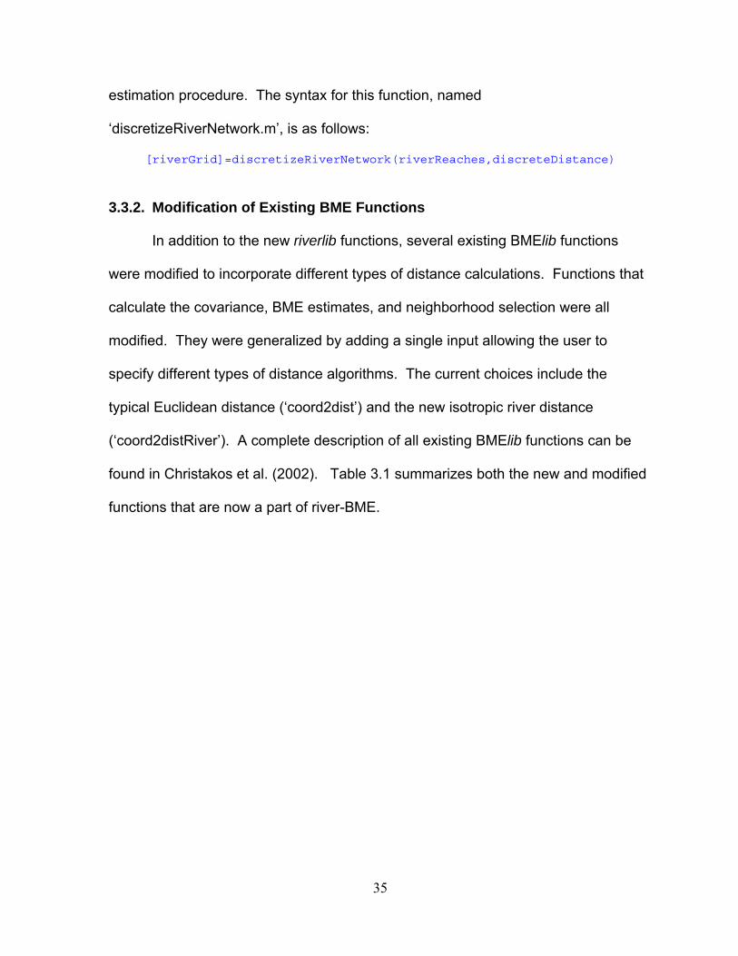
estimation procedure. The syntax for this function, named
‘discretizeRiverNetwork.m’, is as follows:
[riverGrid]=discretizeRiverNetwork(riverReaches,discreteDistance)
3.3.2. Modification of Existing BME Functions In addition to the new riverlib functions, several existing BMElib functions
were modified to incorporate different types of distance calculations. Functions that
calculate the covariance, BME estimates, and neighborhood selection were all
modified. They were generalized by adding a single input allowing the user to
specify different types of distance algorithms. The current choices include the
typical Euclidean distance (‘coord2dist’) and the new isotropic river distance
(‘coord2distRiver’). A complete description of all existing BMElib functions can be
found in Christakos et al. (2002). Table 3.1 summarizes both the new and modified
functions that are now a part of river-BME.

36
Table 3.1: Summary of new and modified functions integrated into the river-BME framework
riverlib PROCESSING Functions
getRiverTopology Obtains the topology for a given network, this includes branching level, reach length, and reach IDs
getRiverStats Calculates total # of reaches, total reach length, Meandering Ratio, Branching Level, and River Ratio
riverlib DISTANCE Functions coord2distRiver Uses the river algorithm to calculate isotropic
river distances between pairs of points cartesian2riverProj Translates traditional space/time locations into
river space/time locations riverlib VISUALIZATION Functions
plotRiverNetwork Produces a picture of a river network including the river topology
discretizeRiverNetwork Produces an equidistant river estimation/mapping grid from a set of river reaches
BMElib MODIFIED Functions
pairsindex Finds pairs of points separated by a given distance interval
coord2K Produces a covariance/variogram matrix from coordinates
coord2Kinterface Interface for calling coord2K
simuchol Generates simulated values
stcov Calculates the space/time covariance for pairs of points
neighbors Selects the hard data estimation neighborhood
probaneighbors Selects the soft data estimation neighborhood
BMEprobaMomentsXvalidation Performs a cross-validation estimation
BMEprobaMoments Calculates BME estimates at a set of space/time locations
3.4. Efficacy of river-BME
3.4.1. Parameter Choice There are a variety of factors that can influence whether the use of a river
distance is appropriate when estimating water quality. These range from the type of
water quality variable, the density of data points, to the complexity of the network.
The first thing to consider when deciding between using a river distance as opposed

37
to more traditional Euclidean distance, is the actual variable under investigation.
Water quality is inherently influenced by both in-stream processes and overland
processes that affect the spatial and temporal distribution of these variables on a
basin-wide scale. If it is determined through empirical evidence that a particular
variable is primarily influenced by factors outside the constraints of a river network,
then using a river distance may not be an accurate representation of the physical
and chemical processes in the true system. For example, tetrachloroehtylene (PCE)
is a widely detected volatile organic compound in water systems. However,
according to several studies, PCE contamination in surface waters is heavily
influenced by leaching from groundwater, storm runoff, and other non-point sources
(Lopes and Bender, 1998; Moran et al., 2002; Akita et al., 2008). These
mechanisms are adequately characterized using Euclidean distances and may
therefore not be constrained by the river network. In this case, a river distance may
not improve the accuracy of water quality estimation and mapping. On the other
hand, variables such as mercury in fish tissue are primarily restricted to the water
column and therefore autocorrelation between fish samples is dependent on the
network configuration. In this case, the use of a river distance may significantly
improve overall estimation and mapping accuracy. In general, however, the
physical, chemical, and biological factors that contribute to the true spatiotemporal
trends of any given water quality parameter are complex. The system is affected by
numerous inputs, both in-stream and overland, therefore a generalized framework
that allows for multiple distance measures is an important contribution of this work.

38
3.4.2. Data Density Another factor to consider when using river distances is the spatial versus
temporal density of hard and soft data points available in the study area. If a
particular study area has very few data points arranged at large distances from one
another in space, then the autocorrelation functions and estimation maps may not be
affected significantly by the choice of a distance measure. In addition, if those same
points are temporally abundant (i.e. lots of measurements taken over time at few
sparse spatial locations), the spatiotemporal estimation neighborhood will be more
informed by (and therefore be biased towards) temporal neighbors rather than
spatial neighbors, causing any spatial distance metric to be less influential in the
BME estimation, and leading to maps that are not significantly different from one
another. However, even if the distance measure has little effect in these situations,
the use of the river-BME framework may still lead to overall better estimates in low
data density situations. A study by Chaplot et al. (2005) examined the effects of
spatial data density on the accuracy of various interpolation techniques on point
height data for digital elevation model (DEM) generation and found that kriging
estimates were more accurate for low data density areas. Other comparison studies
have shown similar results (Dirks et al., 1998; Kravchenko, 2003). Kriging is
considered a linear limiting case of the more general BME methodology (Christakos
and Li, 1998).

39
3.4.3. Measures of Network Complexity In addition to parameter choice and data density, another important
consideration is the geographical complexity of the river network itself. There are
numerous ways to classify basin complexity, including order, meandering ratio, and
drainage density (Strahler, 1952; Julien, 2002; Gordon et al., 2004; Reis, 2006).
This section focuses on a modification of order number we term branching level, and
meandering ratio. A series of tests were performed examining the relationship
between these measures of complexity and the efficacy of using the river distance
developed in this work. For this purpose, the efficacy, E, is defined as the
percentage change in mean square error (MSE) between river-BME (MSEr) and
Euclidean-BME (MSEe).
1001
e
r
MSE
MSEE where (3.1)
n
iobserveditrueier YY
nMSE
1
2,,/ )(
1 (3.2)
where n is the total number of points, and observeditruei YY ,, is the difference between
estimated values and measured values, or the estimation error. Therefore a positive
value for E is equal to the same percentage increase in mapping accuracy. For
example, if when comparing river estimates to Euclidean estimates, the MSEr is 1.0
and the MSEe is 2.0, then the MSE for river-BME is 50% smaller than that of
Euclidean-BME, which we say is resulting in an increase in efficacy of 50%, or

40
stated another way, the estimation accuracy increased by 50% when using a river
distance.
3.4.3.1. Branching Level
Branching level (BL) is similar to the ‘order number’ concept, with the
modification that the most downstream reach is assigned a BL = 1. Each time a
reach at a particular branching level divides into two reaches, the branching level
increases by 1. Figure 3.2 shows an example branching level classification.
Generally speaking, the higher the branching level, the more complex the network.
Figure 3.2: Example of branching level designation for a river network.
In order to test how branching level affects the efficacy of using a river distance over
a Euclidean distance, an actual river network was obtained and simulated values
were re-estimated using either river-BME or traditional BME. The network
configuration for the Raritan Basin in New Jersey was obtained from the New Jersey

41
Department of Environmental Protection (NJDEP) to serve as an example (Figure
3.3).
Figure 3.3: The Raritan Network in New Jersey. This network is used in the branching level, meandering ratio, and simulation tests that follow.
The network was divided into various sub-networks with differing branching
levels. There were a total of 32 different sub-networks, with BL = {1, 2, …, 32}.
Values were simulated using river distances on each sub-network individually and a
cross-validation performed using a Euclidean distance, to determine a MSE for
each. The cross-validation was repeated for the same simulated data using the river
distance. In addition each simulation procedure was repeated 14 times, with the
resulting average efficacy shown as a function of branching level in figure 3.4. The
bars represent the standard deviation among the 14 repeated measurements at
each branching level. The lower bounds are connected to provide a conservative
estimate of efficacy.

42
0
5
10
15
20
25
30
35
40
45
50
1 2 3 4 5 6 7 8 9 10 11 12 13 14 15 16 17 18 19 20 21 22 23 24 25 26 27 28 29 30 31 32
Branching Level
Eff
ica
cy
(%
)
Figure 3.4: Average Efficacy (Eq. 3.2) as a function of branching level in the Raritan basin, New Jersey, with positive standard deviations. Efficacy is defined as the % change in mapping accuracy.
Results of this cross-validation analysis suggest that at extremely low
branching levels, one can expect little change in mapping accuracy when using a
river metric. This is understandable since at very low branching levels the river
network corresponds essentially to a single reach, and as a result there are little
differences between the Euclidean distance and river distance between points.
However, as the branching level increases, the efficacy tends to increase until it
reaches a fairly constant plateau above a branching level of about 5. This cross
validation analysis indicates that using river distances should result in estimates that
are 10 to 45% more accurate than estimates obtained using Euclidean distances for
water quality parameters dominated by in-river processes on river networks with a
branching level greater than 5.
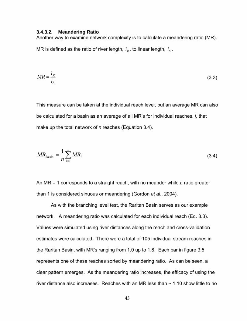
43
3.4.3.2. Meandering Ratio Another way to examine network complexity is to calculate a meandering ratio (MR).
MR is defined as the ratio of river length, Rl , to linear length, Sl .
S
R
l
lMR (3.3)
This measure can be taken at the individual reach level, but an average MR can also
be calculated for a basin as an average of all MR’s for individual reaches, i, that
make up the total network of n reaches (Equation 3.4).
n
iiba MR
nMR
1sin
1 (3.4)
An MR = 1 corresponds to a straight reach, with no meander while a ratio greater
than 1 is considered sinuous or meandering (Gordon et al., 2004).
As with the branching level test, the Raritan Basin serves as our example
network. A meandering ratio was calculated for each individual reach (Eq. 3.3).
Values were simulated using river distances along the reach and cross-validation
estimates were calculated. There were a total of 105 individual stream reaches in
the Raritan Basin, with MR’s ranging from 1.0 up to 1.8. Each bar in figure 3.5
represents one of these reaches sorted by meandering ratio. As can be seen, a
clear pattern emerges. As the meandering ratio increases, the efficacy of using the
river distance also increases. Reaches with an MR less than ~ 1.10 show little to no

44
difference in estimation accuracy when using a river distance. Like with branching
level, this can be expected because reaches with a low MR are essentially straight
lines, therefore any distance calculation along the river would be equal to a
Euclidean distance. However, as the MR increases, the mapping accuracy
increases significantly, by as much as 62% in reaches with extremely high MRs.
0
10
20
30
40
50
60
70
1.01 1.02 1.02 1.04 1.07 1.09 1.11 1.12 1.15 1.21 1.25 1.30 1.32 1.36 1.40 1.50 1.69 1.87
Meandering Ratio
Eff
icac
y (
%)
Figure 3.5: Efficacy (Eq. 3.2) as a function of individual reach meandering ratio in the Raritan Basin, New Jersey. From this analysis it is evident that many factors influence the efficacy of
using a river metric in the geostatistical estimation of water quality. Parameter
choice, data density, and network complexity all play a role in determining how well
river-BME will perform over the traditional space/time framework. Each of these
things should be considered when applying non-traditional distance metrics to
estimation along river networks. The last phase of the numerical implementation of
river-BME is to test its functionality in a series of simulation tests. The final section

45
in this chapter details the results of these tests and sets the stage for the application
of river-BME to real world applications.
3.5. Using river-BME in Simulated Case Studies
3.5.1. Case study using data simulated on a synthetic stream reach In order to validate the use of a river metric within the river-BME framework,
several simulation exercises were performed to gauge the effect a river distance
may have on the estimation and mapping of water quality. The simulation
experiments involved two scenarios. The first scenario involves simulated (i.e.
geostatistically generated) data on a synthetic stream reach. The synthetic stream
reach consists of an idealized sinusoidal curve with a high MR, which maximizes the
potential effects of river distances. Given this synthetic reach, the data are then
simulated using a geostatistical simulation algorithm that generates data having a
prescribed (known) covariance function using river distances. This leads to the
creation of a dataset of simulated (true) values, which can be separated into a
training set (used as monitoring data) and a validation set (where the estimation will
be performed using the training set). The monitoring data from the training set can
be used with river-BME to model the covariance using both distance metrics, as well
as for estimation at the points corresponding to the validation sets (where re-
estimated values obtained using the training set can be compared with the “true”
values in the validation set). Finally, cross-validation or validation statistics are
calculated to compare mean square error results obtained using both river and
Euclidean distance metrics.

46
Figure 3.6 depicts the estimation maps obtained using this simulation scenario. Row
A shows the data that were geostatistically generated and represents the ‘truth’. The
validation set selected from these simulated data consists of two rows of points, one
along the top of the reach, the other along the bottom (within the horizontal bars in
figure 3.6). The validation set values were then re-estimated using the remaining
(training set) data points. The re-estimation obtained using Euclidean distances is
shown in row B, while the re-estimation obtained using river distances is shown in
row C.
Figure 3.6: Simulated data set (row A), estimated using Euclidean-BME (row B) and river-BME (row C). Panel 1 and 2 highlight two areas of distinction between estimates described in the text.
As can be seen in figure 3.6, the Euclidean estimation (row B) creates clouds
of similar values that do not follow the pattern of the ‘true’ data shown on row A,

47
whereas the river (row C) estimated values follow more closely that pattern for this
synthetic stream reach. Panels 1 and 2 in figure 3.6 highlight areas where using the
river based estimation drastically outperforms the Euclidean-based estimation in
reproducing the ‘true’ dataset.
Figure 3.7 shows a scatter plot of simulated (‘true’) values versus estimated
values obtained using Euclidean -BME (panel A) or using river-BME (panel B). An
apparent reduction in scatter is visible when comparing panel A to panel B, leading
one to conclude that the river-BME framework produced more accurate estimates.
This is verified by calculating the MSE using both approaches. The MSEe
(Euclidean) = 0.4866 while the MSEr = 0.2334. One way to quantify the effect of
using river distances versus Euclidean distances is to calculate the efficacy defined
in Eq. (3.1). The efficacy calculated here indicates that the use of river-BME resulted
in a 52% improvement in estimation accuracy over the classical Euclidean-BME
approach.

48
Figure 3.7: Simulated ‘True’ values vs. estimated values using Euclidean-BME (A) and river-BME (B) on a synthetic stream reach.
3.5.2. Case study using data simulated on a real river network The second simulation scenario examines the efficacy of river-BME using a
simulated dataset generated on a real river network (instead of an idealized stream
reach). The real river network used in this case study consists, again, in the New
Jersey Raritan river network (figure 3.3). Simulated values were generated with a
geostatistical simulation method using river distances. Then these simulated values
were used in a cross validation analysis to obtain a MSE for both river-BME and
Euclidean-BME. As explained earlier, the MSE is calculated based on cross
validation errors consisting in the difference between each true value and the value
re-estimated based on its neighboring data. Figure 3.8 depicts the relative scatter
between true values and re-estimated values obtained using Euclidean-BME (panel
A) and river-BME (panel B). The MSE obtained using the data simulated on the
Raritan river basin were similar to those obtained in the previous section, with an

49
MSEe = 0.3030 and MSEr = 0.1624. This corresponds to a 46% improvement in
estimation accuracy (Eq. 3.1) when using river distances instead of Euclidean
distances.
Figure 3.8: Simulated ‘true’ values vs. estimated values using Euclidean-BME (A) and river-BME (B) on a real river network configuration.
Overall these results suggest that the use of a river distance can markedly
improve the estimation accuracy of water quality parameters that are governed by
in-stream processes . However, there are a number of factors that affect the
efficacy of using river-BME instead of Euclidean-BME, and simulated data and
synthetic river networks can only provide a partial examination of the efficacy of
river-BME. Therefore the following chapters provide three real world case studies
that examine the river-BME methodology as it relates to various water quality
parameters and in several real-world river networks. These case studies will provide
a more complete understanding of the differences between river-BME and

50
Euclidean-BME, and will establish the methodology for use in other real world
situations.

Chapter IV: Modern Space/Time Geostatistics Using River Distances: A Case Study of Dissolved Oxygen
4.1. Introduction
Understanding surface water quality is a critical step towards protecting
human health and ecological stability. Because of resource deficiencies and the
large number of river miles needing assessment, there is a need for a methodology
that can accurately depict river water quality where data do not exist. The objective
of this research is to implement such a methodology that incorporates a river metric
into the space/time analysis of dissolved oxygen data for two impaired river basins
using the river-BME framework describes in the previous chapters. We find that
using a river distance in a space/time context leads to an appreciable 10% reduction
in the overall estimation error, and results in maps of DO that are more realistic than
those obtained using an Euclidean distance. As a result river distance is used in the
subsequent non-attainment assessment of DO for two impaired river basins in New
Jersey.
The identification of impaired river segments is a significant requirement of
the federally implemented Clean Water Act (CWA) of 1972. The CWA requires
states to assess water quality and identify and report those segments that are
impaired for particular uses. Dissolved Oxygen (DO) content is one of the easiest
and most basic water quality parameters to measure and is a good indicator of

52
overall stream health. Because of resource deficiencies, budget constraints, and the
sheer number of river miles to be assessed, there is a need for cost efficient and
effective methods that can estimate DO for a large number of river miles using
limited monitoring data.
As mentioned previously, there have been several recent studies regarding
the use of non-Euclidean distances and stream flow in water quality estimation, and
the development of corresponding permissible covariance models (Ver Hoef, 2006;
Cressie et al., 2006; Peterson and Urquhart, 2006; Curriero, 2006; Bailly et al., 2006;
Bernard-Michel and Fouquet, 2006; Peterson et al., 2007). Ver Hoef (2006), Cressie
et al. (2006), and Peterson et al. (2006) demonstrate the use of flow-weighted
covariance models using nitrates, change in DO, and dissolved organic carbon
(DOC), respectively.
A summary of the most recent studies that compare Euclidean and river
covariance models is presented in Table 4.1.
Table 4.1: Water quality estimation studies using river covariance models
Study Water
Quality Parameter
Comparison % Change in MSE1
Model used in
Estimation
Cressie et al. (2006)
Change in DO
Euclidean vs. flow-weighted
Not Reported Euclidean
Peterson & Urquhart (2006)
DOC Euclidean vs. flow-weighted
Exponential Cov.: + 31.3% Spherical Cov: - 9.0% Mariah Cov.: + 32.4%
Euclidean
Ver Hoef et al.
(2006) Sulfate
Isotropic river vs. flow-weighted
Exponential Cov with Constant Mean.:
- 5.5% Flow-Weighted
1 % change in Mean Square Error (MSE). A negative value means that using a flow-weighted covariance model reduces prediction error.
The methods proposed in this work are based on geostatistical principle, most
notably the spatial autocorrelation between data points. They are not meant to take

53
the place of mechanistic and process-based models such as the traditional Streeter-
Phelps or the Qual2 models developed by EPA. Geostatistical models can
complement these existing methods by taking the outputs of these models and using
them as inputs into a geostatistical framework to create larger spatial and temporal
coverages of the parameter of interest, possibly leading to more accurate maps
(LoBuglio et al. 2007). This study attempts to look at only geostatistical models in
order to gain an understanding of the influences that distance measures have on our
ability to assess rivers for DO impairments. Future work will examine the use of
these models in combination with other mechanistic modeling approaches.
While the majority of studies have focused on purely spatial estimation
methods, this research will examine the use of a river metric in a composite
space/time analysis. Since very few studies have used a river metric to examine DO
in a spatial context, and even fewer have done such analysis in a space/time
context, the two objectives of this study are (1) to determine whether the use of a
river metric provides a better model for estimation of DO along a river network in a
space/time context, and (2) to apply the most appropriate space/time model to
estimate DO non-attainment for two impaired river basins based.
4.2. Materials and Methods
4.2.1. Study Area The two study watersheds are shown in Fig. 4.1 together with the locations of
stations that monitored DO at least once during the study period.

54
Figure 4.1: Lower Delaware Basin (left) and Raritan Basin(right), with corresponding locations of monitoring stations with at least one measured DO value (circles). Both areas are high priority basins for the state and have impairments related to
nutrients, sediments, micro-organisms, and DO. The state of New Jersey is divided
into 20 watershed management areas (WMA). The Raritan consists of three WMAs,
the North and South Branch, Millstone, and Lower Raritan. The land uses in both
basins are primarily urban or agricultural. Overall, the Raritan is 36% urban, 19%
agriculture, with the remaining divided between forest, wetland, and water. The
Lower Delaware is 46% urban and 21% agricultural. These classifications are based
on the 1995/97 Land Use/Land Cover designations by the State of New Jersey.
New Jersey has a generally moderate climate with cold winters and warm, humid
summers. These fluctuations in temperature play an important role in determining
the amount of available DO found in these basins. Additionally, both the Lower
Delaware and Raritan basins are geologically structured such that highlands situated
to the west (Raritan) and east (Lower Delaware) feed into flat, highly developed

55
areas near the basin outlets, where impervious surfaces exceed 50% in many
places (NJDEP, 2002). Urban development taking place in both of these basins
over the last two decades coupled with relatively little change in agricultural uses
produces a wide array of point and non-point sources in both regions. This leads to
increased nutrient levels from waste water discharge, urban runoff, and agricultural
runoff, and the potential for higher biological oxygen demand (BOD) and reduced
DO levels. According to the 2006 integrated water quality report, only 5% of
statewide impairments were due to dissolved oxygen, however, greater than 30% of
river miles went un-assessed due to insufficient data (NJDEP, 2006b). This is where
methods such as the one employed in this study become increasingly important.
4.2.2. Dissolved Oxygen Data DO data were obtained from two sources for the period beginning January 1,
1990 through August 1, 2005. The first source is the U.S. Geological Survey
(USGS) National Water Information System (NWIS). The second source is the
USEPA storage and retrieval (STORET) database. Often times these databases
report values with clarifying symbols accompanying them to signify uncertainty in the
measurement. Therefore, in order to use these values in the analysis, any value
reported as ’less than’ a particular value (i.e. containing a ‘<’ in the database) were
treated as equal to 50% of that value , and values reported as estimated (i.e.
containing an ‘E’ in the database) were treated as actual values. A summary of the
data are given in Table 4.2.

56
Table 4.2: Basic Statistics for monitored DO data (raw-mg/L) for the period January, 1990 – August, 2005 for the Raritan and Lower Delaware river basins in New Jersey
Parameter Raritan Basin Lower Delaware Basin # of Space/Time Data Points 1755 1855# of Monitoring Stations 65 47Mean (mg/L) 10.471 7.859Variance (mg/L) 7.061 5.359Skewness Coefficient -0.006 0.306Kurtosis Coefficient 2.462 2.437
4.2.3. Space/Time Covariance Modeling Using River Distance As noted in § 2.4 the exponential power model for covariances using isotropic
river distances has been proven permissible. Therefore, for this study and the
subsequent case studies, we are restricted to this class of covariance functions.
The flow-weighted covariance function is not considered here because very few
points during a given day of the study period are flow-connected, and as Peterson
and Urquhart (2006) suggest, using a flow-weighted covariance in this situation can
lead to less informative maps. This analysis uses a space/time random field
(S/TRF) X(p), where p=(r,t) is a space/time point, r is the spatial river coordinate and
t is time. The covariance cx(p,p’) of X(p) is said to be spatially isotropic/temporally
homogeneous if it can be expressed in terms of the spatial distance r=d(r,r’) and the
time difference =|t-t’|. Experimental values of the covariance for a spatial distance r
and temporal lag are obtained using a covariance statistical estimator on pairs of X
measurements approximately separated by the spatial distance r, and temporal lag
. The parameters of a covariance model are then adjusted until a best fit is found
between the model and experimental covariance values. The covariance model
used in this analysis is given by:

57
....3
exp3
exp)()(),(22
21
tr aa
rcrcrc
444
333
3exp
3exp
2cos
3exp
trtr aa
rc
aa
rc
(4.1)
where r is chosen to be either the Euclidean or river distance and is the nugget
coefficient in space or time . This model consists of 4 structures where c1…c4 are
calculated portions of the total variance and correspond to the coefficients of each
structure (i.e. c1 for structure 1, c2 for structure 2…). The first term of each structure
is the spatial component, while the second term relates to the temporal component
of the covariance. The variables ar and at are the spatial and temporal ranges for
each structure. Other than the initial nugget, the spatial component of the remaining
structures is exponential, which as shown above is permissible for any directed tree
river network for the Euclidean and river distances, and therefore the overall model
is permissible because it corresponds to nested space/time separable permissible
covariance functions (Kolovos et al., 2004). The temporal component is exponential
for structures 2 and 4, while structure 3 is a cosinusoidal function related to the
seasonal fluctuations often associated with DO. Further covariance details are
found in section 4.3.1.
4.2.4. Estimation of Dissolved Oxygen
The river-BME and Euclidean-BME methods were used to estimate DO at un-
sampled river locations. BME provides a rigorous mathematical framework to

58
process a wide variety of knowledge bases characterizing the space/time distribution
and monitoring data available for DO, and obtain a complete stochastic description
of DO at any unmonitored space/time point in terms of its posterior Probability
Distribution Function (PDF), as discussed in Chapter 2.
The distribution of DO across space and time is modeled as the sum of a
non-random function mDO(p) and an isotropic/stationary residual S/TRF X(p). The
spatial and temporal components of mDO(p) were obtained by exponential smoothing
of the time-averaged and spatially-averaged data, respectively. The non-random
function mDO(p) describes the modeled spatial and temporal trends of DO, while the
S/TRF X(p) captures the residual space/time variability and uncertainties.
The site specific knowledge includes both hard data (e.g. measured value) and soft
data (i.e. data with associated measurement error). By way of summary, BME uses
the maximization of a Shannon measure of information entropy and an operational
Bayesian updating rule to process the general and site specific knowledge bases,
and obtain the posterior PDF describing the DO concentration at any un-sampled
point of the river network (Christakos et al., 2002).
This research uses the special case where only hard data are considered (i.e. the
measurement errors are small or unidentified). In this case the BME method yields
the estimators of linear geostatistics known as the simple, ordinary and universal
kriging methods. This research, therefore, is based on a form of space/time linear
kriging.
In order to determine which of the Euclidean or river metrics was more
accurate for the assessment of DO in the study basins, a cross-validation procedure

59
was used. Each data point was removed sequentially and re-estimated using the
remaining space/time data points. The Mean Square Error (MSE) is calculated as
the sum of the squared differences between re-estimated and measured values.
The method with the lowest MSE is then used in the assessment of DO along
unmonitored rivers.
Using the selected distance metric within the river-BME framework we
estimate DO at equidistant estimation points (i.e. distributed at a fixed interval of 0.1
miles) along the Raritan and Lower Delaware river networks. Monitoring data are
treated as hard data because all measurements met the USGS or EPA data quality
standards. For each estimation point the hard data situated in its local space/time
neighborhood is selected, and the corresponding BME posterior PDF is calculated to
describe DO at that estimation point. The BME posterior PDF obtained at equidistant
points along the river network are then used to obtain estimated DO values, which
are used to produce maps of DO concentration, and delineate river miles that may
be impaired.
4.2.5. Assessment of Impaired River Miles
In order to better understand the seasonal pattern of DO impairment and
better quantify the probability of these impairments, a criterion-based space/time
assessment framework is employed to categorize the fraction of river miles meeting
certain probability thresholds, as discussed in Akita et al. (2007). These thresholds
give us the ability to classify the probability of violation of a standard for any
space/time estimation point based on its BME posterior PDF. The standard for DO

60
concentration was set at 7 mg/L, which is the standard used by NJDEP for FW-TP
streams (NJDEP, 2006a). Using this standard, the probability of violation at
space/time point p is then defined as the probability that the BME mean estimate is
> 7 mg/L, i.e.
Prob[Violation,p]=Prob[DO(p)>7.0mg/L] (4.2)
The fraction of river miles impaired during any given time period is calculated using
the fraction of equidistant estimation points for which the probability of violation is in
excess of some pre-selected probability threshold.
4.3. Results & Discussion
4.3.1. Covariance of DO in New Jersey
Fig. 4.2 shows the experimental covariance values (squares) obtained using
the mean trend removed DO data for the Raritan and Lower Delaware River Basins.
These estimates were then used to fit the non separable space/time covariance
model (Eq. 4.1). The sills c1,…, c4, spatial ranges ar2, ar3, ar4, and temporal ranges
at2, at3, at4 obtained are listed in Table 4.3, and the resulting model is shown as a
solid line in Fig. 4.2.
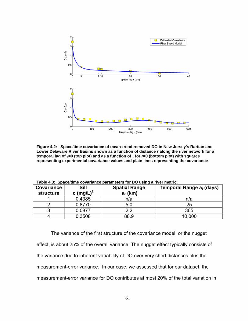
61
Figure 4.2: Space/time covariance of mean-trend removed DO in New Jersey’s Raritan and Lower Delaware River Basins shown as a function of distance r along the river network for a temporal lag of =0 (top plot) and as a function of for r=0 (bottom plot) with squares representing experimental covariance values and plain lines representing the covariance
Table 4.3: Space/time covariance parameters for DO using a river metric. Covariance structure
Sill c (mg/L)2
Spatial Range ar (km)
Temporal Range at (days)
1 0.4385 n/a n/a 2 0.8770 5.0 25 3 0.0877 2.2 365 4 0.3508 88.9 10,000
The variance of the first structure of the covariance model, or the nugget
effect, is about 25% of the overall variance. The nugget effect typically consists of
the variance due to inherent variability of DO over very short distances plus the
measurement-error variance. In our case, we assessed that for our dataset, the
measurement-error variance for DO contributes at most 20% of the total variation in

62
the data, which is within the upper bound indicated by the nugget effect. The
second structure of the covariance model contains a short range exponential spatial
component and a short range exponential temporal component. Fluctuations of DO
over this combination of short spatial ranges (5 km) and short temporal ranges (25
days) may be due to local sources of pollution acting over short spatial distances
(such as point pollution discharges leading to local increase of BOD and subsequent
reductions in DO over short distances) that either have intermittent pollution
discharge loading lasting just a few days, or are persistent but have an effect that is
altered intermittently by meteorology events lasting from a few days to a month (e.g.
rainfall events, or changes in temperature which significantly effects the oxygen
saturation of water). This accounts for nearly 50% of the overall variation. The third
structure of the covariance also contains a very short range exponential spatial
component but coupled with a medium range cosinusoidal hole temporal component
with a periodicity corresponding exactly to a calendar year. This covariance
structure contributes approximately 5% of the total variation in DO and corresponds
to processes acting seasonally. These processes are very localized geographically
as they act over distances of about 2.2 km, which may again include localized spikes
in BOD and subsequent DO depletion, as well as the natural variability in river
morphology and processes acting on DO over distances ranging from of 1 to 3 km.
The final covariance structure consists of a long range exponential component in
both space and time. The long spatial range of 88.9 km can be attributed to
characteristics and impacts from non-point source pollution from suburban
development and agricultural runoff that can affect long stretches of rivers at once.

63
What is interesting to note is that these fluctuations have a temporal range of about
10,000 days or 27.4 calendar years, which captures time scales corresponding to
long term effects of human activities and impact on the environment, as well as
climatic changes that may alter the air/water interface and oxygen equilibrium. It
should be recognized that there is a wider confidence interval for this temporal range
than for any of the other spatial or temporal ranges of our covariance model because
this temporal range of 27.4 years exceeds the duration of the time period for which
data are available (15 years). Nonetheless it is interesting to note that it is a very
large temporal range, which suggests that non-point source pollution over large
geographical areas may have an impact on DO that is lasting much longer than the
impact of point source pollutions. This may have the serious policy implication that,
while pollution prevention strategies may have quick responses in abating the effect
of point sources pollution, these strategies may face a much greater challenge in
abating rapidly the effect of non-point source pollution on the DO in the surface
waters of New Jersey.
4.3.2. Euclidean vs. River Estimation
A cross-validation was performed to examine the differences in estimation of
DO using a Euclidean versus a river distance. Table 4.4 summarizes the cross-
validation MSE obtained for each river basin using both distances.

64
Table 4.4: Change in cross validation mean square error (MSE) for each basin. A negative change indicates a reduction in overall MSE (i.e. improvement) when using a river metric.
Basin Euclidean MSE River MSE % Change in
MSE
Raritan 1.7381 1.5416 - 11.3%
Lower Delaware 1.3193 1.1836 - 10.3%
The use of a river metric resulted in 11.3% (Raritan) and 10.3% (Lower Delaware)
decrease in MSE. We note that the cross-validation points were at a distance from
their neighboring training data points corresponding to several times the average
spatial and temporal ranges. In this situation there isn’t as much contrast between
the Euclidean and river metrics as would be the case if the points were closer across
space. Hence, it is possible that the true gain in mapping accuracy is higher than the
10%-11% found. This is supported by other cross-validation analysis we conducted
using synthetic datasets (results not shown here). The approximately 10% reduction
in estimation error is appreciable because previous studies using river distance in an
estimation context found little difference between a Euclidean and river based model
and in some cases found a river distance to increase the prediction error (Ver Hoef
et al., 2006; Cressie et al. 2006; Peterson et al., 2006; Peterson et al., 2007).
The improvement in mapping accuracy is supported by our covariance
analysis. The variance weighted average of the Euclidean and river spatial ranges
were 9.7km and 20.4km, respectively. This means that DO levels are correlated over
much longer distances along the river network than across land. This is due in part
to the fact that a river meanders, so that the distance along two points is longer
along the river reach than across land. The ratio of river distance to straight-line
distance between two reach endpoints is known as the meandering ratio (MR).

65
However, even when we account for the meandering of the network, the range of
correlation between points along a river network is significantly higher than when
using a Euclidean metric. For example, the average (MR) for both the Lower
Delaware and Raritan basins is approximately 1.2. Factoring out this effect by
dividing the ratio of river range to Euclidean range (2.1) by the average MR (1.2)
gives us an adjusted ratio of river vs. Euclidean range of 1.8. This means that, in
practice, even after adjusting for meandering, the correlation along the river is still
1.8 times longer than across land.
While use of the river metric produces maps of DO that are more accurate
than those obtained using a Euclidean metric, one might ask whether these maps
are visually different. The visual difference can best be shown by comparing the DO
estimated in two areas of the Raritan Basin, as shown in Fig. 4.3. The maps
obtained using a Euclidean metric are shown on the left, while the maps obtained
using the river metric are shown on the right. The subfigure contains the zoomed in
portion of the northwestern Raritan basin corresponding to the North and South
Branch WMA to highlight two major differences when comparing metrics. Fig. 4.3(a)
depicts the zonal differences while Fig. 4.3(b) depicts the parallel reach effect.

66
Figure 4.3: Zonal (a) and Parallel Reach effect (b) on the BME Estimation of DO Residual in the Upper & Lower Branch Raritan Basin on Dec 16, 2002 using a Euclidean metric (left) or a river metric (right). Squares are locations of monitoring stations for this time period and the solid lines indicate the WMA boundary.
From Fig. 4.3(a) the differences in zonal influence that points have when using a
Euclidean vs. a river metric are apparent. This is directly connected to the
differences in covariance ranges. The river covariance has a longer variance
weighted spatial range, resulting in a larger zone of influence of data points along
the river. For the Euclidean metric this zone is circular in nature with a smaller range
than the zone of influence observed with the river metric, as can be seen by
comparing the right and left maps of Fig. 4.3(a). Fig. 4.3(b) depicts another
phenomenon along parallel reaches. When estimating the DO level at a point along
an unmonitored reach, a higher relative weight is assigned to a sample collected at a
point that is at a short distance along the river network, than at a point that is at a

67
short distance across land. So when considering the case shown in Fig. 4.3(b)
where two clearly different river branches are running in parallel of one another, we
see that the Euclidean map on the left tends to propagate information from the
monitoring data point across land, while the river map on the right constrains the
propagation of that information to the river branch where the sample was collected,
leading to a more realistic map where parallel branches have distinct water quality.
Given the monitoring data available in this study, the results support our hypothesis
that the river metric provides more accurate and realistic maps of DO across a river
network than maps obtained using a Euclidean metric. Based on this conclusion,
river distance was incorporated into the estimation of DO in the Raritan and Lower
Delaware River Basins for a subset of the study period (2000-2005) to improve our
assessment of the fraction of river miles not attaining the FW-TP standard for DO in
New Jersey.
4.3.3. River-BME Estimation of DO Using the river metric the BME posterior PDF was calculated describing DO
at estimation points distributed uniformly along all river miles of in the Raritan and
Lower Delaware Basins. Fig. 4.4 depicts the BME mean estimate of DO on June 12,
2002. This date is representative of a typical summer month where DO is at its
lowest in both basins. The darker areas highlight river miles where DO has fallen
below the New Jersey FW-TP standard of 7 mg/L. The inset highlights an area in
the southeast quadrant of the Raritan Basin, corresponding to the Millstone WMA
where a majority of river miles are impaired for DO during this time period.
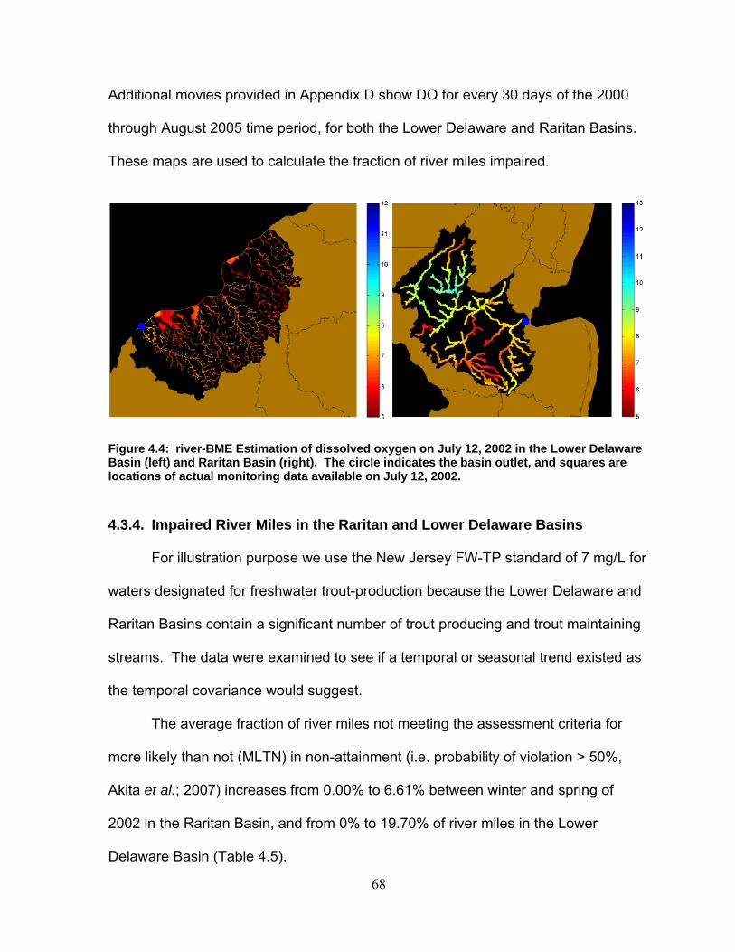
68
Additional movies provided in Appendix D show DO for every 30 days of the 2000
through August 2005 time period, for both the Lower Delaware and Raritan Basins.
These maps are used to calculate the fraction of river miles impaired.
Figure 4.4: river-BME Estimation of dissolved oxygen on July 12, 2002 in the Lower Delaware Basin (left) and Raritan Basin (right). The circle indicates the basin outlet, and squares are locations of actual monitoring data available on July 12, 2002.
4.3.4. Impaired River Miles in the Raritan and Lower Delaware Basins
For illustration purpose we use the New Jersey FW-TP standard of 7 mg/L for
waters designated for freshwater trout-production because the Lower Delaware and
Raritan Basins contain a significant number of trout producing and trout maintaining
streams. The data were examined to see if a temporal or seasonal trend existed as
the temporal covariance would suggest.
The average fraction of river miles not meeting the assessment criteria for
more likely than not (MLTN) in non-attainment (i.e. probability of violation > 50%,
Akita et al.; 2007) increases from 0.00% to 6.61% between winter and spring of
2002 in the Raritan Basin, and from 0% to 19.70% of river miles in the Lower
Delaware Basin (Table 4.5).

69
Table 4.5: Seasonal Average Variation in Fraction (%) of River Miles More Likely than Not (MLTN) in Non-Attainment (probability of Violation > 50%) for 2002
Season Fraction of Raritan
Impaired (% river miles)
Fraction of Lower Delaware Impaired (%
river miles) Winter (Jan-Mar) 0.00 0.00Spring (Apr-Jun) 6.61 19.70Summer (Jul-Sep) 23.47 57.92Fall (Oct-Dec) 0.00 0.04
In the summer of 2002, this fraction of impaired river miles increases even further, to
about 23% in the Raritan and about 58% in the Lower Delaware. Much of this
phenomenon can be related to temperature changes depending on season. In the
warmer months, water temperature is at its highest and therefore does not hold as
much oxygen as the colder water in the winter months. Because New Jersey, and
particularly the Raritan sit at higher latitudes, the water temperature drops drastically
in winter, leading to near 0% of river miles being impaired. Alternatively, the warmer
waters of the summer and spring can foster biological growth that consumes large
amounts of DO. This increase in BOD compounds the effects of higher
temperatures and leads to more river miles in non-attainment.
From 2000 to 2005, between about 8% to 58% of river miles were found to be
MLTN in non-attainment in the warmer summer months (Table 4.6).
Table 4.6: Average Summer Fraction (%) of River Miles More Likely than Not (MLTN) in Non- Attainment (probability of Violation > 50%) for the period 2000-2005 (Summer = Jul- Sep).
Date Fraction of Raritan
MLTN Impaired (% river miles)
Fraction of Lower Delaware MLTN
Impaired (% river miles) Summer 2000 6.86 10.03Summer 2001 14.21 57.00Summer 2002 23.47 57.92Summer 2003 12.68 13.77Summer 2004 12.44 34.01Summer 2005 19.40 43.87

70
The fraction of impaired river miles was highest in 2002, that fraction decreased in
2003 and 2004, but it increased again in the last year of our study period, 2005,
indicating that low DO may be an on-going problem in these basins. 2005 was also
the warmest summer on record in New Jersey and coupled with a drought, could
have contributed to the increase in impaired river miles. An analysis was also
conducted to determine the fraction of river miles highly likely in non-attainment (i.e.
probability of violation > 90%, Akita et al.; 2007). Based on this criterion, we found
that the Lower Delaware had a much higher fraction of river miles ascertained as
impaired than can be found in the Raritan. Over the study period, the Lower
Delaware had as much as 19% of river miles highly likely in non-attainment, while
the Raritan remained around 1.8%. DO itself is affected by a number of
environmental factors, including temperature, salinity, nutrient levels and biological
oxygen demand. One reason for explaining the larger percentage of impaired miles
in the Lower Delaware is the fact that not only is the percentage of urban area
larger, but the overall amount of agricultural land is also larger than that in the
Raritan, possibly contributing non-point source nutrient loading into adjacent
streams. Land cover and land use have shown to greatly impact the quality of
streams and rivers, especially in areas undergoing rapid conversion to more urban
development patterns (King et al., 2005; Chang, H. 2008).
One of the limitations of this approach is the exclusion of other parameters
that can be used to predict DO levels. DO is affected by the geochemistry of the
water, and therefore process-based models may provide additional information to
refine our geostatistical models. Additionally, this approach looks at only one class

71
of potential covariance functions, the exponential power model, other functions need
to be tested for permissibility when using river distance (isotropic or flow-weighted).
Finally, we use a partial cross-validation procedure to examine the predictive
capability of our model. Full model validation using measured DO will be useful for
further model refinement in future work.
These results suggest that continued DO monitoring is particularly critical in the
Lower Delaware basin to evaluate future trends in DO during the summer months.
There is more work needed, however, to identify the specific causes of low DO. The
DO maps generated provide a general basis to help begin the process of identifying
these causes.
Several conclusions can be drawn from the results of this study. First, our
implementation of a river distance metric in the BMElib package provides an efficient
and flexible tool for the space/time analysis of DO along river networks. Second,
application of river-BME to analyze DO in two river basins in New Jersey lead to
maps that are about 10% more accurate and appreciably more realistic than maps
obtained using the classical Euclidean distance. In addition it was found that after
adjusting for river meandering, the correlation of DO along the river is about 1.8
times longer than across land and DO non-attainment was worse in the Lower
Delaware, over more river miles and over a longer period of time than in the Raritan.
Finally, additional parameters, such as BOD, temperature, salinity, and nutrients
should be factored in to improve estimation accuracy at unmonitored locations.
Chapter V: Modern Space/Time Geostatistics Using River Distances: A Case Study of Turbidity and Escherichia coli
5.1. Introduction This chapter is again an investigation into the use of river-BME for real world
water quality applications. It builds upon the previous case study by incorporating
soft data into the analysis. This study will be the first use of river distances along
with the integration of hard and soft data for water quality estimation.
5.1.1. Fecal Indicator Bacteria in River Systems Escherichia coli (E.coli) is a widely used indicator of fecal contamination in
water bodies. External contact and subsequent ingestion of bacteria coming from
fecal contamination can lead to harmful health effects. Since E.coli data are
sometimes limited, the objective of this study is to use secondary information in the
form of turbidity to improve the assessment of E.coli at un-monitored locations. We
obtained all E.coli and turbidity monitoring data available from existing monitoring
networks for the 2000 – 2006 time period for the Raritan River Basin, New Jersey.
Using collocated measurements we developed a predictive model of E.coli from
turbidity data. Using this model, soft data are constructed for E.coli given turbidity
measurements at 739 space/time locations where only turbidity was measured.
Finally, the Bayesian Maximum Entropy (BME) method of modern space/time
73
geostatistics was used for the data integration of monitored and predicted E.coli data
to produce maps showing E.coli concentration estimated daily across the river basin.
The addition of soft data in conjunction with the use of river distances reduced
estimation error by about 30%. Furthermore, based on these maps, up to 35% of
river miles in the Raritan Basin had a probability of E.coli impairment greater than
90% on the most polluted day of the study period.
Fecal indicator bacteria (FIB) provide important health and ecological
information for many river basins. Although FIB’s themselves are not harmful, their
presence in streams suggests that pathogenic microorganisms might also be
present, leading to possible human health risks. Diseases and illnesses that can be
contracted in water with high fecal contamination include typhoid fever, hepatitis,
gastroenteritis, and dysentery (Mallin et al., 2000). The most commonly tested FIBs
are total coliforms, fecal coliforms, Escherichia coli (E.coli), and enterococci. E.coli
is a species of fecal coliform that is specific to fecal material from humans and other
warm blooded animals. Based on studies conducted by the Environmental
Protection Agency (EPA), E.coli is the best indicator of health risk from water contact
in recreational waters (USEPA, 2000). Therefore many states are now measuring
E.coli instead of total coliforms to assess streams for fecal contamination. However,
due to the limited scope of existing monitoring networks, budget limitations, and
manpower constraints, it is difficult to assess all river miles. The purpose of this
study is to examine the use of a modern spatiotemporal geostatistics technique,
known as Bayesian Maximum Entropy (BME), to statistically assess E.coli’s
presence in both monitored and un-monitored streams using not only existing E.coli

74
data but also integrating secondary information in the form of turbidity
measurements to further improve the mapping of basin-scale fecal indicators.
5.1.2. Autocorrelation in E.coli
Geostatistical techniques such as kriging rely on the fact that many natural
phenomenon exhibit spatial autocorrelation. Monitoring stations along the same
stream, for example, tend to report similar physical and chemical characteristics.
Kriging methods construct a regional model of correlation to estimate variables, such
as E.coli, at un-sampled locations based on data from sampled locations
(Delhomme, 1978; Cressie, 1990; Stein, 1999). Cokriging, subsequently, uses not
only the spatial correlation of a single variable, but also the correlations associated
with other environmental variables. There have been numerous examples of
cokriging for environmental variable estimation ranging from soil salinity, suspended
sediment, and rainfall, to regional stream quality (Darwish et al., 2007; Li et al.,
2006; Seo et al., 1990; Jager et al., 1990). It is most beneficial where the primary
variable is under-sampled with respect to the secondary variable, as is the case for
this study when examining E.coli and turbidity as secondary information. Generally
the inclusion of secondary information results in more accurate local predictions than
when considering a single variable alone (Darwish et al., 2007; Goovaerts, 1997).
A more general approach, and the approach used in this study, to estimating at un-
sampled locations is the BME method of modern space/time geostatistics
(Christakos and Li, 1998). As described in Chapter 2, this method accounts for both
spatial and temporal correlations between data points. The major component of this

75
study is to determine whether the use of river-BME along with turbidity as a
secondary variable, improves our estimation of E.coli for un-monitored stream
reaches.
5.1.3. Turbidity and E.coli
Turbidity is the measure of light attenuation in a water column. It is related to
E.coli concentration in that research has shown that FIBs are oftentimes associated
with particulate matter in the water column and transport of fecal bacteria via
suspended sediments is an important aquatic mechanism (Mallin et al., 2000; Sayler
et al., 1975). Often-times bacteria will settle out of the water column into the
sediment. The sediment can become entrained and allow the release of particulate
matter and the associated bacteria. Additionally, as bacteria concentration
increases, the amount of light absorbance in water also changes. Numerous studies
have examined the relationship between turbidity and E.coli and found significant
correlation between both parameters (Adams et al., 2007; Dorner et al., 2007; Vidon
et al., 2008; Reeves et al., 2004). Our study area contained a larger number of
measured turbidity values relative to E.coli, therefore turbidity was chosen as a
secondary variable.
5.2. Materials and Methods
5.2.1. Data and Study Area Like the previous case study, the area under investigation is the Raritan River
Basin in north-central New Jersey (Figure 5.1). The basin is 1100 square miles and

76
consists of 36% urban, 19% agriculture, 27% forest, and approximately 17%
wetland/water land uses. Approximately 1.2 million people live within this basin and
both fecal coliforms and turbidity have been cited as major resource concerns
(NJDEP, 2002). Water quality data for the Raritan Basin was obtained through the
National Water Information System (NWIS), maintained by the United States
Geological Survey (USGS) for the period January 1, 2000 – December 30th, 2007. A
total of 44 monitoring stations provided 579 space/time data points for measured
E.coli while 118 monitoring stations yielded 739 measurements of turbidity for the
study period. E.coli data were log-normally distributed with a mean of 5.4 log-colony
forming units (cfu)/100mL. Figure 5.1 summarizes the locations of E.coli and
turbidity measurements during the study period.
Figure 5.1: Locations of at least one E.coli (large circle) and turbidity (small circle) measurement between 2000-2007 in the Raritan Basin, New Jersey.

77
5.2.2. Generation of Soft Data One of the primary goals of this research is to introduce a secondary variable,
in the form of turbidity, to predict E.coli concentrations in areas where there are no
direct E.coli measurements. These predicted values are referred to as ‘soft’ data
because of the uncertainty associated with the predicted values. There are two
types of soft data employed in this study, probabilistic and interval. To construct the
probabilistic soft data, we used a total of 27 locations where both turbidity and E.coli
were measured. Using these collocated points a simple linear regression was
performed using log-transformed data to determine an initial correlation (r-squared =
0.54) which was consistent with other studies relating turbidity to E.coli or fecal
coliform concentration (Adams et al., 2007; Dorner et al., 2007; Vidon et al., 2008;
Reeves et al., 2004). Because of the limited number of collocated points and
relatively low values of turbidity represented, the final least squares predictive model
for E.coli is a continuous piecewise function containing the linear relationship along
with a polynomial model of order 2 to reduce overestimation of E.coli at extremely
high turbidity values :
Log-E.coli=
6.057.105.2
6.008.202.007.2 2
zz
zzz (5.1)

78
where log-E.coli is expressed in log-cfu/100mL, and log-turbidity (z) is expressed in
log-NTU. Using this relationship the log-E.coli prediction error variance was
calculated using the mean of the squared differences between predicted and
measured log-E.coli for a series of given windows of log-turbidity values. Finally, for
every space/time point where log-turbidity (but not necessarily log-E.coli) was
measured, a Gaussian probability distribution function (PDF) was constructed for
log-E.coli with a mean given by (1) and a variance corresponding to the prediction
error variance at the measured log-turbidity. This resulted in soft log-E.coli data of
Gaussian probabilistic type at 739 space/time points.
The uncertainty associated with the direct measurements of low levels of
E.coli was also accounted for. The data downloaded from the USGS uses the
membrane filtration (m-Tec) method for bacteria enumeration and several
intercalibration studies suggest 0.5 log as a working point to account for
measurement error (Noble et al., 2003; Griffith et al., 2003). Therefore, for any
measured log-E.coli < 2 log-cfu/100mL in this study, an interval soft datum was
introduced in the general form of equation (5.2). This resulted in an additional 15
soft data points.
Prob[a<log-E.coli<b]=1 (5.2)
5.2.3. Integrating Hard and Soft Data To integrate the soft data with the measured log-E.coli values and then
estimate at un-monitored locations, the BME method of modern space/time

79
geostatistics is used (see Chapter 2). As described in previous sections, both the
river-BME and Euclidean-BME procedure consists of defining the general knowledge
(i.e. covariance), site specific knowledge (i.e. monitoring data), and integrating the
two to calculate a posterior PDF (Eq. 2.5). In this case study, site specific
knowledge includes both hard data (e.g. measured values) and soft data (i.e. log-
E.coli predictions based on turbidity).
5.2.4. Space/Time Covariance Modeling Using River Distance As with the previous case study, a covariance model is selected that uses
river distances and we restrict our model choice to the exponential power model
since it has been shown to be permissible when using river distances (see Chapter
2, § 2.4, and Appendix A). In the case of log-E.coli in the Raritan Basin, considering
a spatial range equal to the area of the basin itself, on average only 1.6 data points
were flow-connected. Therefore an isotropic covariance model was chosen to
estimate log-E.coli in the Raritan Basin. The final model used in this study for the
space/time covariance of log-E.coli between space/time points p=(r,t) and p’=(r’,t’) is
cov(p,p’)=
333
222
111
3exp
3exp
3exp
3exp
3exp
3exp
trtrtr aa
hc
aa
hc
aa
hc
(5.3)
where t and t’ are times, and h=d(r,r’) and =|t-t’| are the spatial and temporal lags,
respectively. In this study we used either =0 (Euclidean distance) or =1 (river
distance).

80
5.2.5. Comparing Euclidean and River Estimations
A comparison was made between estimations using river distance, as
described above, and estimation using the typical Euclidean distance, alongside the
incorporation of soft data from measured turbidity. Cross-validation tests were
performed on three different scenarios to determine the best model for estimating
basin-wide log-E.coli. Scenario 1 used the measured log-E.coli data (i.e. the 15
interval soft data points and all the hard data) with the Euclidean distance. Scenario
2 contained the same data as scenario 1 except the river distance was used.
Scenario 3 built upon scenario 2 by adding in the turbidity data (incorporated as the
soft Gaussian data constructed using Eq. 1). The method with the lowest MSE was
then used in the assessment and estimation of E.coli for the entire Raritan Basin.
5.2.6. Estimation of E.coli
Using the selected distance metric within the BME framework we estimate
E.coli at equidistant estimation points (i.e. distributed at a fixed interval of 0.1km)
along the Raritan River Basin network. For each estimation point we select the hard
and soft log-E.coli data situated in its local space/time neighborhood, and calculate
the corresponding BME posterior PDF describing log-E.coli at that estimation point.
The variance of the BME posterior PDF provides an assessment of the estimation
uncertainty, while the back-log transform of the mean of the BME posterior PDF is
used as an approximation of the median estimator for E.coli concentrations. This is

81
then used to produce chloropleth maps of estimated E.coli concentration, and
delineate river miles that are more-likely-than-not impaired.
5.2.7. Assessment of Impaired River Miles In order to better understand the pattern of fecal contamination impairment
and better quantify the probability of these impairments, a criterion-based space/time
assessment framework is used to categorize the fraction of river miles meeting
certain probability thresholds, as discussed in Akita et al. (2007). These thresholds
give us the ability to classify the probability of violation of a standard for any
space/time estimation point based on the BME posterior PDF of log-E.coli. The
standard for E.coli concentration was set at 235cfu/100mL, which is the standard set
by NJDEP for primary contact recreation. Using this standard, the probability of
violation at space/time point p is defined as the probability that E.coli>235cfu/100mL,
i.e.
Prob.[Violation,p]=Prob.[E.coli(p)>235cfu/100mL] (5.4)
The fraction of river miles impaired on any given day of the study period is then
obtained by calculating the fraction of equidistant estimation points for which the
probability of violation (Eq. 5.4) is in excess of some pre-selected probability
threshold (e.g. 90%).

82
5.3. Results and Discussion
5.3.1. Covariance Analysis Figure 5.2 shows the covariance cX(h,) of log-E.coli obtained for the Raritan
Basin. The top panel displays cX(h,�0) which shows how the covariance varies as
a function of spatial lag h for a temporal lag equal to , while the bottom panel
displays cX(h,) which shows how the covariance varies as a function of temporal
lag for a zero spatial lag.
Figure 5.2: Spatial (top) and temporal (bottom) covariance of log-E.coli in the Raritan Basin, New Jersey.
Experimental covariance values estimated from data are shown with markers, while
the covariance models obtained by fitting Eq. 5.3 to the markers are shown with
lines. The covariance was calculated and modeled using both a Euclidean distance

83
(dashed line) and river distance (plain line). The covariance model parameters
obtained with the Euclidean and river distances are summarized in table 5.1.
Table 5.1: E.coli Space/Time Covariance Model Parameters
c1
(*)
ar1
(km) at1
(days) c2
(*)
ar2
(km) at2
(days) c3
(*)
ar3
(km) at3
(days)
Euclidean 1.35 30 80 1.08 100 200 0.27 200 500
River 1.35 40 80 1.08 300 200 0.27 400 500
(*) c1, c2, c3 are expressed in (log-cfu/100mL)2
The first structure of the covariance model (with parameters c01, ar1 and at1) is
similar for both Euclidean and river distance-based models, with 50% of the total
variability of log-E.coli being characterized by a fairly short range of 30-40km in
space and 80 days in time. This is not inconsistent with variability we would expect
from point-like sources of E.coli pollution that are not constant and therefore may
dissipate over a few months. The second and third structures of both Euclidean and
river covariance models indicate that the remaining 50% of variability in log-E.coli
levels is autocorrelated over longer distances and durations. As noted before, E.coli,
and fecal bacteria in general, is oftentimes associated with suspended sediment in
the water column. This sediment can travel longer distances along a river network
and it is hypothesized that E.coli associated with suspended sediment remains in the
water at high levels for a longer period of time than free bacteria. This phenomenon
is captured in the longer spatial and temporal ranges of the covariance models. In
the Euclidean based model, the longer range was between 100-200km in space and
200-500 days in time. Interestingly, for the river based-model, the spatial ranges
were anywhere from 1.5 to 2 times longer (300-400km), suggesting that by

84
accounting for the river connections between points, E.coli concentrations may
remain correlated over much longer distances than previously considered.
5.3.2. Cross-validation Analysis The cross-validation analysis outlined above resulted in mean square errors
of MSE1=2.87(log-cfu/100mL)2 for scenario 1, MSE2=2.57(log-cfu/100mL)2 for
scenario 2, and MSE3=1.99(log-cfu/100mL)2 for scenario 3. Comparing scenario 1 to
scenario 2 we see that by using river distances instead of Euclidean distances we
reduce the estimation error by about 10%, which is similar to the reduction found in a
previous study examining dissolved oxygen in the Raritan Basin (Money et al.,
2008). If we then add in soft log-E.coli data derived from measured turbidity
(scenario 3), there is an additional 24% decrease in estimation error. Therefore by
incorporating river distances along with soft data from turbidity, the estimation error
was reduced by 31% when compared to log-E.coli estimation using the typical
Euclidean distance and no secondary information. This is one of the first instances
in a space/time context that river distances and secondary information have been
combined to significantly reduce estimation error. As a result, the river-based
covariance model was deemed to be the most accurate representation of E.coli in
the Raritan Basin, and was used in the subsequent basin-wide estimation and
mapping of fecal contamination.

85
5.3.3. Assessment of Fecal Contamination in the Raritan Basin Median estimates of E.coli concentration were calculated for every day of the
study period between 2000-2007. A movie showing changes in these estimated
concentrations over time and space can be viewed in Appendix D. Figure 5.3
depicts the E.coli concentration for 4 different days of and is representative of many
of the days in this study. The squares indicate locations of monitoring stations with
measured E.coli values and the chloropleth map shows areas where the
concentration exceeds the single sample standard of 235cfu/100mL.
Figure 5.3: river-BME estimation of E.coli in the Raritan Basin, New Jersey on 8/16/02 (A), 2/14/03 (B), 5/14/03 (C), and 8/16/05 (D).

86
One can see from these maps and the animation that extremely high E.coli
concentrations (> 600cfu/100mL) can be found along the eastern side of the basin in
the North and South Branch and Lower Raritan watershed management areas
(WMA). Over the last half of the study period the Lower Raritan WMA remained
consistently contaminated with E.coli well above the state standard for contact
recreation. In addition, several hot spots could be identified in the upper Millstone
WMA that would appear and then dissipate, suggesting the occurrence of acute
point source contamination in those areas. It should also be noted that high E.coli
concentrations were estimated in many areas where no monitoring stations existed.
In these areas, additional monitoring strategies may be needed to capture potential
harmful levels of E.coli.
It is also important to assess the confidence in these estimations and
describe the probability that a particular river mile is impaired for E.coli. This
information is important for decision-makers and environmental managers when
deciding how to allocate resources and devise public warnings of fecal
contamination. Using the log-E.coli posterior PDF calculated at regularly spaced
estimation points along the Raritan, we calculated for each day of the study period
the percentage of river miles with a probability of impairment (Eq. 5.4) greater than
90%. Figure 5.4 depicts these results for a 300 day window of the study period.

87
Figure 5.4: Percentage of river miles in the Raritan Basin that have a 90% probability of violating the NJDEP standard for primary contact recreation over a 300 day period.
The x-axis is the day of estimation and the y-axis is the percentage of river
miles in the Raritan Basin that exceeded the standard with 90% confidence. The
fraction of river miles having a >90% probability of being impaired was highly
variable from one day to another, and reached a maximum of 35% on the most
polluted day of this time period.
Overall this study provides a unique spatiotemporal framework for
incorporating river distances and secondary information into the basin-wide
assessment of water quality. Accuracy has been improved by over 30% when
combining river distances and turbidity as an indicator of E.coli concentration. By
constructing our model in this way, we are better able to estimate E.coli along un-
monitored stream segments, thereby increasing the overall number of river miles
assessed and providing environmental managers with accurate maps that not only
show the spatial and temporal distribution of E.coli but that can also highlight areas

88
of concern, which can be useful when evaluating future monitoring strategies and
allocating resources.
89
Chapter VI: Modern Space/Time Geostatistics Using River Distances: A Case Study on Fish Tissue Mercury
6.1. Introduction This study continues to build on the previous applications of river-BME for
water quality estimation. As with the previous case studies, this chapter examines
the differences in estimation using either river-BME or Euclidean-BME. It extends
the analysis presented in Chapter 5 by incorporating multiple sources of soft data
(pH and surface water mercury) for the estimation and mapping of fish tissue
mercury in the Cape Fear and Lumber basins in North Carolina.
6.1.1. Mercury in the Environment
Mercury (Hg) is a naturally occurring substance that is present in air, water,
and sediments as a result of both anthropogenic and natural sources. Due to the
reactive chemical nature of mercury, it can change forms depending on the media it
comes into contact with. The mercury cycle has been developed to organize the
various avenues with which mercury can enter the environment (Morel et al., 1998).
Mercury is naturally present at ambient levels in the atmosphere. Additional
atmospheric mercury is due to emissions from volcanoes and fossil fuel burning.
This mercury undergoes photochemical oxidation and is deposited through
precipitation where it is then allowed to runoff into lakes and streams. Once in the
water, inorganic mercury will settle into the sediments, while some mercury remains
in the water column and is converted to methylmercury by bacteria present in the

90
water. Methylmercury is a highly toxic substance that is readily bioaccumulated by
aquatic organisms (Porcella, 1995). It is the bioaccumulated methylmercury that
poses the most risk to human health. The majority of mercury enters the human
body through fish consumption (USEPA, 1997a; 1997b). This poses a significant
risk because methylmercury can penetrate mammalian cells and alter cell division,
putting children and pregnant women at a much larger risk than the general
population. Methylmercury can affect the nervous system and in high doses can
affect the kidneys and cardiovascular system (Watras et al., 1998; National
Research Council, 2000). There have been numerous studies on mercury
distribution in ecosystems, including air (Mason et al., 1997; Fulkerson and Nnadi,
2006), surface water (Balogh et al., 1997; Sullivan and Mason, 1998), and fish tissue
(Kannan et al., 1998; Peterson and Sickle, 2007).
Many states and local agencies monitor fish tissue mercury and use this
information to issue consumption advisories for particular areas and species of fish.
Assessing the spatiotemporal trends of fish tissue mercury on a larger scale, based
on monitoring data is a difficult task. Inter-species variability, such as trophic level,
and intra-species variability such as size or age have an impact on the amount of
bioaccumulated mercury present in a system (Huckabee et al., 1979; MacCrimmon
et al., 1983; Cope et al., 1990; Wiener and Spry, 1996). In 2006, in the United
States alone, 38% of total lake acreage and 26% of all river miles had fish
consumption advisories (USEPA, 2007).
91
6.1.2. Autocorrelation of Fish Tissue Mercury
Geostatistical techniques such as kriging rely on the fact that many natural
phenomenon exhibit spatial autocorrelation. Kriging methods construct a regional
model of correlation to estimate variables at un-sampled locations based on data
from sampled locations (Delhomme, 1978; Cressie, 1990; Stein, 1999). Cokriging,
subsequently, uses not only the spatial correlation of a single variable, but also the
correlations associated with other environmental variables. There have been
numerous examples of cokriging for environmental variable estimation ranging from
soil salinity, suspended sediment, and rainfall, to regional stream quality (Darwish et
al., 2007; Li et al., 2006; Seo et al., 1990; Jager et al., 1990). It is most beneficial
where the primary variable is under-sampled with respect to the secondary variable.
Generally speaking, the inclusion of secondary information results in more accurate
local predictions than when considering a single variable alone (Darwish et al., 2007;
Goovaerts, 1997).
A more general approach, and the approach used in this study, to estimating
at un-sampled locations is the BME method of modern space/time geostatistics
(Christakos and Li, 1998). The BME method provides a rigorous mathematical
framework to process a wide variety of knowledge bases. These Knowledge Bases
characterize the space/time distribution and uncertainty in monitoring data available
for various water quality parameters, and are used to obtain a complete stochastic
description of these parameters at any unmonitored space/time point in terms of its
posterior Probability Density Distribution (PDF). The major component of this study

92
is to determine whether the use of river-BME along with several types of soft data
can improve our estimation of fish tissue mercury at un-sampled locations.
As noted before fish tissue mercury can vary significantly due to inter and
intra-species variability. Therefore, distinguishing between the natural
spatiotemporal trends and species specific trends can be difficult if the monitoring
data are heterogeneous (i.e. contains many different species). Wente (2004)
describes an interesting approach to this problem by developing a statistical model
for distinguishing trends in fish tissue mercury concentration using a combination of
covariance and multiple linear regression. This model serves as the basis for the
Environmental Mercury Mapping, Modeling, and Analysis (EMMMA) program (Hearn
et al., 2006). Although it is not the focus of this work, EMMMA results could be
integrated into the river-BME analysis, potentially leading to more accurate maps of
fish tissue mercury distribution. For our purposes, however, we are focusing on the
inclusion of river distances for the geostatistical estimation of fish tissue mercury to
understand its distribution on a basin scale and across several species. (see § 6.2).
6.1.3. Factors Influencing the Bioaccumulation of Mercury
A major contribution of this work is the incorporation of secondary variables in
the form of soft data that effect the concentration of mercury in fish tissue. A number
of studies have examined a variety of water quality variables and their relationship to
fish tissue mercury. Many found that one of the best predictors of fish tissue
mercury is pH (Grieb et al., 1990; Rose et al., 1999; Song et al., 2001; Sackett et al.,
2008). Low pH values have been shown to increase the amount of methylmercury

93
released from sediments, increasing its bioavailability (Ullrich et al., 2001; Miller and
Akagi, 1979). Oftentimes measurements such as pH are more readily available than
fish tissue samples, therefore it is a good candidate for generating soft data for fish
tissue mercury in areas where fish samples do not exist.
The majority of mercury enters from outside the water body, and ultimately a
large majority becomes associated with sediments; however, some mercury remains
in its elemental form in the water column, where it is directly transformed into
methylmercury by bacteria. Surface water measurements for mercury are typically
very scarce and difficult to measure, resulting in large datasets with values below the
detectable limit of the procedure being used. The USEPA (2001) suggests the use
of bioaccumulation factors (BAF), or the ratio of fish tissue mercury to water column
mercury (WCHg), to determine the appropriate levels of aqueous mercury that would
result in compliant fish tissue mercury concentrations. Minute concentrations of
aqueous mercury are capable of generating methylmercury at rates significant
enough to warrant consumption advisories (Southworth et al., 2004). Therefore,
this study incorporates additional soft data for fish tissue mercury derived directly
from surface water mercury measurements, rather than a BAF, which are more
reliable if site-specific.
6.2. Materials and Methods
6.2.1. Data and Study Area
The area under investigation is the Cape Fear and Lumber river basins in
eastern North Carolina. Both of these basins have ongoing fish consumption
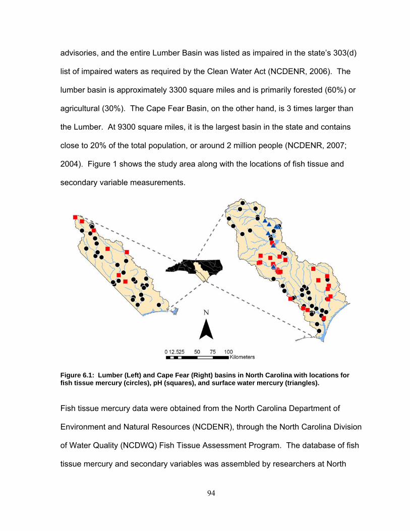
94
advisories, and the entire Lumber Basin was listed as impaired in the state’s 303(d)
list of impaired waters as required by the Clean Water Act (NCDENR, 2006). The
lumber basin is approximately 3300 square miles and is primarily forested (60%) or
agricultural (30%). The Cape Fear Basin, on the other hand, is 3 times larger than
the Lumber. At 9300 square miles, it is the largest basin in the state and contains
close to 20% of the total population, or around 2 million people (NCDENR, 2007;
2004). Figure 1 shows the study area along with the locations of fish tissue and
secondary variable measurements.
Figure 6.1: Lumber (Left) and Cape Fear (Right) basins in North Carolina with locations for fish tissue mercury (circles), pH (squares), and surface water mercury (triangles). Fish tissue mercury data were obtained from the North Carolina Department of
Environment and Natural Resources (NCDENR), through the North Carolina Division
of Water Quality (NCDWQ) Fish Tissue Assessment Program. The database of fish
tissue mercury and secondary variables was assembled by researchers at North

95
Carolina State University, and a complete description of this database can be found
in Sackett et al. (2008). Only those data within the Cape Fear and Lumber Basins
were used. Collocated pH data and fish tissue mercury were obtained from this
database and additional pH measurements were downloaded from the National
Water Information System through the United States Geological Survey (NWIS-
USGS). Surface water total mercury data included data collected by NCDWQ as
part of the Eastern Regional Mercury Study (NCDWQ, 2003, 2006), as well as
additional data from the NWIS. Any duplicate measurements were averaged to a
single value. Table 1 summarizes the data used in this study.
Table 1: Data summary for mercury and pH in the Cape Fear and Lumber basins, 1990-2004
Data Type # of Locations# of space/time data
points # collocated with
Fish Hg* Fish Hg 75 1663 - pH 33 356 143 Surface Water Hg**
7 80 35
*Independent from space/time data locations in column 3; **starts in 1995
6.2.2. Generation of Soft Data from Multiple Sources
The availability of secondary variables provides an opportunity to incorporate
additional soft data points for fish tissue mercury. Money et al. (2008) described the
general framework for generating soft data from secondary water quality variables
by creating E.coli soft data from turbidity measurements. However; that study
focused on only one source of soft data. In this study we incorporate two secondary
variables, pH and surface water mercury to generate probabilistic soft data and
combine them into one analysis.
There were a total of 143 points where both fish tissue mercury (FishHg) and
pH were measured. Using these collocated points, a simple regression analysis was

96
performed using log-transformed data to create a relationship of predicted FishHg
given pH (Eq. 6.1).
log-FishHg = -3.5 log-pH + 5.7 (6.1)
where log-FishHg is expressed in log-mg/kg (or ppm) and log-pH is in log-standard
units. Using this relationship the log-FishHg prediction error variance was calculated
using the mean of the squared differences between predicted and measured log-
FishHg for a series of given windows of log-pH values. Finally, for every space/time
point where log-pH (but not necessarily log-FishHg) was measured, a Gaussian
probability distribution function (PDF) was constructed for log-FishHg with a mean
given by (1) and a variance corresponding to the prediction error variance at the
measured log-turbidity. This resulted in soft log-FishHg data of Gaussian
probabilistic type at 356 space/time points.
There were a total of 35 points where both fish tissue Hg and water column
mercury (WCHg) were measured during the study period. Again, using these
collocated points, we constructed a simple relationship to predict fish tissue Hg using
log-transformed data.
log-FishHg = 0.25 log-Hgsw – 3.40 (6.2)
where log-FishHg is as above expressed in log-mg/kg (or ppm) and log-WCHg is
expressed in log-ng/L. For every space/time location where surface water mercury

97
was measured, a Gaussian probability distribution function was constructed for log-
FishHg with a mean given by (2) and variance corresponding to the prediction error
variance at the measured log-WCHg. This resulted in soft log-FishHg data of
Gaussian type at an additional 80 space/time locations.
The models shown in equations 6.1 and 6.2 are simplified expressions of a
complex system that has many potential secondary variables. As discussed earlier,
a variety of factors effect the concentration of mercury in fish tissue, however the
intent of this study is to examine how the addition of soft data in conjunction with a
river distance affects the estimation accuracy of fish tissue mercury, therefore a
simplified model was most appropriate. Future research will examine more complex
models for predicting fish tissue and examine ways to incorporate those model
predictions as soft information.
6.2.3. Integrating Hard and Soft Data
The site specific knowledge for log-FishHg comes from direct measurements
of fish tissue mercury (treated as hard data) and from secondary variables, pH and
surface water total mercury, which are used to construct soft data. The BME method
of modern space/time geostatistics (see Chapter 2-5) is used to integrate these hard
and soft data and obtain statistical estimates of log-FishHg at un-monitored
locations. As described in previous sections, both the Euclidean-BME and river-
BME procedures consist in defining the general knowledge (i.e. covariance) and site
specific knowledge (i.e. monitoring data), and integrating these two knowledge

98
bases to obtain a posterior PDF (Eq. 2.5) characterizing log-FishHg at any point on
the river.
6.2.4. Space/Time Covariance Models That Use River Distances
As with previous water quality studies using river-BME (Money et al., 2008a,
2008b), a covariance model is selected that uses either a Euclidean or river
distance. We restrict our model choice to the isotropic exponential power covariance
model since it has been shown to be permissible when using river distances (Ver
Hoef et al., 2006, Money et al., 2008a). Using this model, the covariance of log-
FishHg between space/time points p=(r,t) and p’=(r’,t’) is expressed as
cov(p,p’) =
222
111
3exp
3exp
3exp
3exp
trtr aa
hc
aa
hc
(6.3)
where t and t’ are times, h=d(r,r’) and =|t-t’| are the spatial and temporal lags,
respectively , and d(r,r’)=dR(r,r’)+(-1)dE(r,r’) (Eq. 2.11) is an -weighted
average of the Euclidean distance dE(r,r’) and the river distance dR(r,r’). In this study
we used either =0 (Euclidean distance) or =1 (river distance). For each value of
, the parameters (c1, ar1, at1, c2, ar2, at2) of the covariance model (6.3) are obtained
using a least square fitting between the covariance function and experimental
covariance values calculated from the hard log-FishHg data. An interpretation of
these parameters is provided in § 6.3.

99
6.2.5. Comparing Euclidean and River Estimations
A comparison was made between estimations using river distance, as
described above, and estimation using the typical Euclidean distance, alongside the
incorporation of soft data from measured pH and measured WCHg. A cross-
validation analysis was performed on five different scenarios to determine the best
model for estimating basin-wide log-FishHg. Scenario 1 used the measured log-
FishHg data with Euclidean-BME. Scenario 2 contained the same data as scenario
1 except river-BME was used. Scenario 3 built upon scenario 2 by adding in the pH
data (incorporated as the soft Gaussian data constructed using Eq. 1). Scenario 4
built upon scenario 2 by adding in Gaussian soft data from WCHg using equation 2.
Finally, scenario 5 combined the soft data from scenarios 3 and 4 into one analysis
using river-BME. The method with the lowest MSE was then used in the
assessment and estimation of FishHg for the Cape Fear and Lumber basins.
Table 6.2 summarizes each scenario.
Table 6.2: Cross-validation scenarios for Fish Tissue Hg estimates using River-BME and Euclidean-BME
Scenario Metric Used Hard Data Used Soft Data Used
I Euclidean Measured log-FishHg
-
II River Measured
log-FishHg -
III River Measured log-FishHg
Gaussian from log-pH
IV River Measured log-FishHg
Gaussian from log-Hgsw
V River Measured log-FishHg
Gaussian from log-Hgsw +
Gaussian from log-pH
6.2.6. Estimation of Fish Tissue Hg

100
Using the selected scenario within the BME framework we estimate log-
FishHg at equidistant estimation points (i.e. distributed at a fixed interval of 0.1km)
along the combined Cape Fear and Lumber network. For each estimation point we
select the hard and soft log-FishHg data situated in its local space/time
neighborhood, and calculate the corresponding BME posterior PDF describing log-
FishHg at that estimation point. The variance of the BME posterior PDF provides an
assessment of the estimation uncertainty, while the back-log transform of the mean
of the BME posterior PDF is used as an approximation of the median estimator for
FishHg concentrations. This is then used to produce chloropleth maps of estimated
FishHg concentration, and calculate the fraction of river miles that exceed specified
action levels.
6.2.7. Assessment of Impaired River Miles
The fraction of river miles impaired at any given time is calculated by
determining the fraction of equidistant estimation points that exceed a given action
level for fish tissue mercury. There are currently three different action levels for fish
tissue mercury. The Food and Drug Administration (FDA) has determined a
consumer action level of 1.0 ppm (or mg/kg) (FDA, 2001). The state of North
Carolina has declared a more stringent action level of 0.4 ppm (Williams, 2006). In
addition, the USEPA has set the most stringent mercury action level at 0.3 ppm
(USEPA, 2001). For the Cape Fear and Lumber basins, the fraction of total river
miles exceeding each of these threshold concentration values was calculated
independently.

101
6.3. Results and Discussion
6.3.1. Covariance Analysis
Figure 6.2 shows the covariance cX(h,) of log-FishHg obtained for the
Raritan Basin. The top panel displays cX(h, 0), which shows how the covariance
varies as a function of the spatial lag h for a temporal lag equal to zero, while the
bottom panel displays cX(h,), which shows how the covariance varies as a
function of temporal lag for a zero spatial lag.
Figure 6.2: Spatial (top) and temporal (bottom) covariance of log-FishHg in the Cape Fear and Lumber Basins, North Carolina. Experimental covariance values estimated from data are shown with markers, while
the covariance models obtained by fitting Eq. 6.3 to the markers are shown with
lines. The covariance was calculated and modeled using both a Euclidean distance

102
(dashed line) and river distance (plain line). The covariance model parameters
obtained with the Euclidean and river distances are summarized in table 6.3.
Table 6.3: FishHg Space/Time Covariance Model Parameters c1
(*)
ar1
(km) at1
(days) c2
(*)
ar2
(km) at2
(days)
Euclidean (=0) 0.38 58 685 0.0001 0.0001 6.16
River (=1) 0.30 111 1070 0.10 114 0.70
*c1 and c2 are expressed in log-ppm2
The first structure of the covariance model (with parameters c1, ar1 and at1)
explains approximately 75% of the overall variability in FishHg using river distance,
and nearly 100% of the variability when using Euclidean distance. The
corresponding spatial range of the first structure using river-BME is nearly double
the spatial range of the Euclidean-BME model. This suggests that by accounting for
river distance, fish tissue mercury is spatially more highly correlated than if the
constraints of the river network are not taken into account. Physically this can be
explained because fish are inherently restricted to following pathways that mimic the
river network configuration. As one would expect, if a Euclidean distance is used,
the correlation between fish can be lost over a short distance because fish do not
generally travel across land. Indeed, the spatial covariance range (ar1) indicates that
95% of the correlation in FishHg is lost after about 58km, compared to 111km when
taking river distance into account. Temporally, fish tissue mercury remains highly
correlated for a period of about 2-3 years. This is understandable given that

103
bioaccumulated mercury will change gradually over time, depending upon the age
and size structure of the fish community.
6.3.2. Cross-validation Analysis
The cross-validation analysis outlined in table 2 resulted in mean square
errors of MSE1 = 0.3050(log-ppm2) for scenario 1, MSE2 = 0.2556 (log-ppm2) for
scenario 2, MSE3 = 0.2480 (log-ppm2) for scenario 3, MSE4 = 0.2508 (log-ppm2) for
scenario 4, and MSE5 = 0.2487 (log-ppm2) for scenario 5. Using river-BME over
Euclidean-BME with only hard data reduced estimation error by (MSE1-
MSE2)/MSE1=16.2%. This is appreciably higher than what was obtained in previous
studies that examined river-BME for DO and E.coli. Those studies resulted in 10%-
11% decrease in error. Also when accounting for soft data from either pH or WCHg
independent of one another, an additional 2-3% reduction in estimation error was
found. Even though this is appreciably smaller than the reduction seen from soft
data in the E.coli study by Money et al. (2008), it is significant because relatively few
soft data points were available in this study. In the E.coli/turbidity study there were
over 700 additional soft data points added to the analysis, and covering a much
smaller land area. In this study, there were only ~300 additional soft data derived
from pH and only ~30 additional soft data points derived from WCHg. The reduction
in estimation error may be even further reduced if more data points can be included
for these secondary variables. The basin under investigation is also very large.
The land area of the Cape Fear and Lumber Basins combined is 4 times the size of
basins used in previous studies. Overall, when using river-BME with one source of

104
soft data (either pH or WCHg), there was an 18.7% reduction in estimation error
when compared to the Euclidean-BME without secondary data. This suggests that
accounting for the hydrogeography of the system as well as variables that affect the
bioaccumulation of mercury, will result in more accurate estimations of fish tissue
mercury at un-sampled locations.
One interesting finding is that when combining the two sources of soft data
(pH and WCHg) into a single estimation, there was no significant decrease in error
when compared to estimations calculated using the sources independently. Again,
one reason for this result is the number of soft data relative to the number of hard
data. There were over 1600 hard data space/time locations and approximately 400
soft data points used in the combined analysis, meaning that for any given
estimation point, the estimation neighborhood is more likely to contain hard data
points with more weight than any soft data point. Additionally, with the distribution of
WCHg measurements concentrated in a small area of the Northeastern Cape Fear
Basin (see figure 1), the estimation neighborhood will likely contain either soft data
from pH, or soft data from WCHg, but rarely would it contain both. This means that
more often than not, any decrease in estimation error can primarily be attributed to
the use of river distance, followed by the inclusion of either source of soft data, but
not both sources of soft data at the same time. Lange et al. (1993) suggested that
acidity may increase the methylation process, and generally speaking water column
total mercury increases the availability of mercury for methylation and subsequent
bioaccumulation in fish, which can explain why pH and WCHg, when considered

105
separately, lead to more accurate maps of FishHg. But it is also possible that pH and
surface water mercury may work together in the uptake of mercury into fish tissue.
For example, Chen et al. (2001) noted that the bioavailable speciation of Hg
and factors that bind with Hg depend on pH. Another possibility is that water column
total mercury is a source of methylmercury in the sediment, and pH may aid the
methylation of mercury at the sediment-water interface (Winfrey and Rudd, 1990).
However, the detailed mechanisms of how the combined effect of water column
mercury and pH affects methylmercury formation and bioaccumulation are still
largely unknown, and our spatially discontiguous datasets for pH and WCHg may
not capture their combined effect. This could help explain why the combination of
soft data from these two sources does not result in any additional decrease in
estimation error in our study.
6.3.4. Assessment of Fish Tissue Mercury
Median estimates of FishHg concentration were calculated every 180 days
over the study period between 1990-2004. A movie showing changes in fish tissue
mercury over space and time can be viewed in supplementary material. Figure 6.3
depicts the FishHg concentration for 4 sample days during the study period.

106
Figure 6.3: river-BME Fish Tissue Mercury estimates (ppm) in the Cape Fear and Lumber Basins on July 23, 1995 (A); July 2, 1999 (B); June 26, 2000 (C); and May 13, 2004 (D). Squares indicate locations of actual fish tissue measurements.
These estimates show that over the course of the study period a large proportion of
both basins had the potential for fish tissue mercury levels to be above both the EPA
and North Carolina action levels (0.3 and 0.4 ppm respectively). Only a small
fraction exceeded the FDA action level of 1.0ppm. Generally the Lumber basin
contained higher potential for contaminate fish over more of the basin and for a
longer period of time. This is reflected by the fact that the entire Lumber basin has
been listed as impaired for fish tissue mercury in the 2006 North Carolina Integrated
Water Quality report (NCDENR, 2007). The area of Jordan Lake in the northeastern

107
Cape Fear also contained high estimates of fish tissue mercury during several time
periods, however, very few actual samples were taken in this area during the study.
One can combine estimation maps and maps of error variance to provide state and
local agencies with a tool for designing future monitoring strategies and better
pinpointing fish consumption advisories in areas like Jordan Lake. Figure 6.4
summarizes the fraction of river miles impaired during the study period.
Figure 6.4: Percentage of river miles with fish tissue mercury median estimate exceeding Mercury Action Levels set by the FDA (top; 1.0ppm), North Carolina (middle; 0.4ppm), and the EPA (bottom; 0.3ppm).
The median estimate of fish tissue mercury exceeded the most stringent
action level of 0.3ppm in more than 90% of river miles for a majority of the study
period. There were more fluctuations in the percent of impaired river miles when the
action level was increased to the current North Carolina level of 0.4ppm; however,
over 50% of river miles had median estimates of fish tissue mercury exceeding
0.4ppm for almost the entire study period. In addition, during the years 1990-1994,
Percentage of river miles

108
between 1-4% of river miles had a median estimate of fish tissue mercury above
even the most lenient action level of 1.0ppm set by the FDA. Another small peak is
seen in 1998; however, at least with respect to the FDA, the majority of waters
remained below this action level, suggesting that measures to mediate mercury
inputs into streams and lakes may be taking effect. No river miles had a median
estimate of fish tissue mercury exceeding the FDA action level since 1999 according
to these results.
Overall this study examines a combination of knowledge sources that may
improve the estimation of fish tissue mercury concentrations in two large river basins
in North Carolina. Estimation maps were produced that were on average 18% more
accurate when accounting for river distance and the secondary variables pH and
water column total mercury. Both secondary variables contributed to an overall
decrease in estimation error, albeit small due to the limited amount of data points
available for these secondary variables. The use of river-BME in this study
contributed a majority of the reduction in estimation error and provides a good
framework for further decreases in estimation error with the addition of other
secondary factors in future work. Soft data from pH contributed as much error
reduction as soft data from surface water mercury. Generally pH data are much
more reliable and easier to measure, therefore state and local agencies may
consider using pH measurements to aid in the assessment of fish tissue mercury in
areas where samples may be scarce. However, this work demonstrates that water
column total mercury data, when available, can provide a valuable alternate source
of information to estimate fish tissue mercury levels. Overall, the framework

109
developed in this work can aid environmental managers in identifying important
bioaccumulation factors and areas where sampling and advisory resources can be
targeted.

Chapter VII: Concluding Remarks
The primary goal of this work was to establish a new framework for estimating
water quality along river networks, using modern space/time geostatistics with a river
distance. In order to achieve this goal the existing Bayesian Maximum Entropy
Framework was extended with new river-based functions and modified functions to
create the new river-BME framework. It was determined that there are several
factors that affect the efficacy of using river-BME for water quality assessments.
These included parameter choice, data density, and network complexity. Network
complexity plays a significant role in determining whether or not a river-based
approach is most appropriate. Both branching level and meandering ratio were
shown to impact the efficacy of using river-BME. Generally speaking, as network
complexity increases, the efficacy of river-BME increases over that of the classical
Euclidean-BME approach. In addition, simulation exercises confirmed that the
numerical implementation of river-BME was successful and established the
framework for use in real world applications.
The real world case studies provide a broad range of applications for using
river-BME. A variety of parameters and network configurations were examined to
illustrate the potential for river-BME to improve estimation accuracy over the
Euclidean based approach. It was hypothesized that by accounting for the
hydrogeography of a system, a noticeable decrease in estimation error would occur
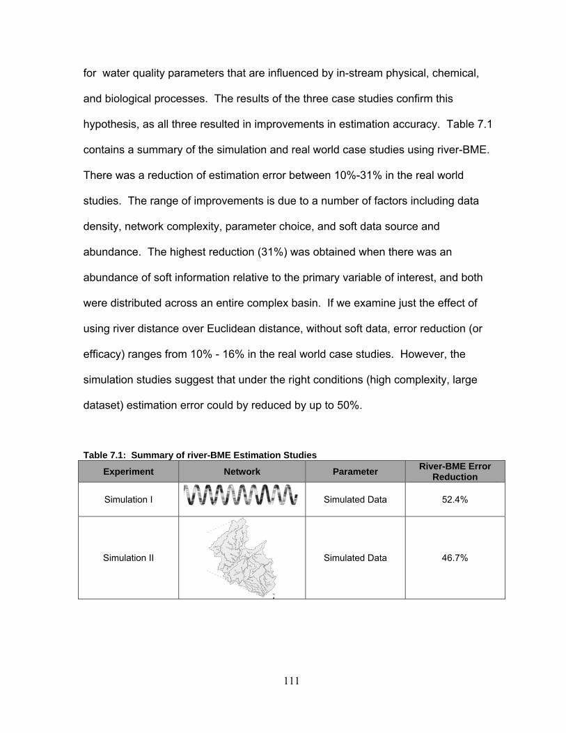
111
for water quality parameters that are influenced by in-stream physical, chemical,
and biological processes. The results of the three case studies confirm this
hypothesis, as all three resulted in improvements in estimation accuracy. Table 7.1
contains a summary of the simulation and real world case studies using river-BME.
There was a reduction of estimation error between 10%-31% in the real world
studies. The range of improvements is due to a number of factors including data
density, network complexity, parameter choice, and soft data source and
abundance. The highest reduction (31%) was obtained when there was an
abundance of soft information relative to the primary variable of interest, and both
were distributed across an entire complex basin. If we examine just the effect of
using river distance over Euclidean distance, without soft data, error reduction (or
efficacy) ranges from 10% - 16% in the real world case studies. However, the
simulation studies suggest that under the right conditions (high complexity, large
dataset) estimation error could by reduced by up to 50%.
Table 7.1: Summary of river-BME Estimation Studies
Experiment Network Parameter River-BME Error
Reduction
Simulation I
Simulated Data 52.4%
Simulation II Simulated Data 46.7%

112
Hard Data Dissolved Oxygen 11.3%
Hard Data Dissolved Oxygen 10.3%
Hard & Soft Data E.coli with soft data
from Turbidity 31.2%
Hard & Soft Data Fish Tissue Mercury with soft data from
pH & WCHg 18.7%
Hard & Soft Data Fish Tissue Mercury with soft data from
pH & WCHg 18.7%
Overall river-BME was able to significantly reduce water quality estimation
error along a variety of river networks and for a variety of parameters. There are
limitations, however, to this approach. First, the algorithm developed for this work
calculated isotropic river distance and does not take into account flow connectivity
between data points. Although the models presented can be generalized to include
a combination of Euclidean and river distance, and flow-weighted covariance models

113
are available and should be incorporated into future work. Second the covariance
functions used in the analysis were restricted to the spatial exponential power model
for =0 (Euclidean distance) and =1 (river distance), which has been proven
permissible for any river networks (see Appendix B). There are a variety of other
possible covariance functions that need to be examined for permissibility before they
can be used in a river-based geostatistical framework. In addition, more complex
models of environmental parameters (i.e. Qual2, EMMMA, CMAQ) can be used to
generate soft data, which may lead to even further improvements in estimation and
mapping of water quality.
Future research directions should examine the use of other types of models
to generate soft data in conjunction with river-BME. Also, more water quality
variables and additional networks with varying complexity need to be investigated for
the efficacy of using river-BME. This will help to establish a general library of
network and variable types and their associated efficacy, which will be an invaluable
tool to future researchers. Other potential extensions for river-BME include areas
where restricted network distances may play a role in the autocorrelation between
points (i.e. water distribution systems). The river-BME framework developed here is
a general tool that sets the stage for a multitude of research regarding
spatiotemporal trends in water quality along river networks. It will provide local,
state, and federal environmental managers with a framework for better targeting
resources, advising stake-holders, and informing the public of water quality trends
and impairments that may affect future ecological and human health.
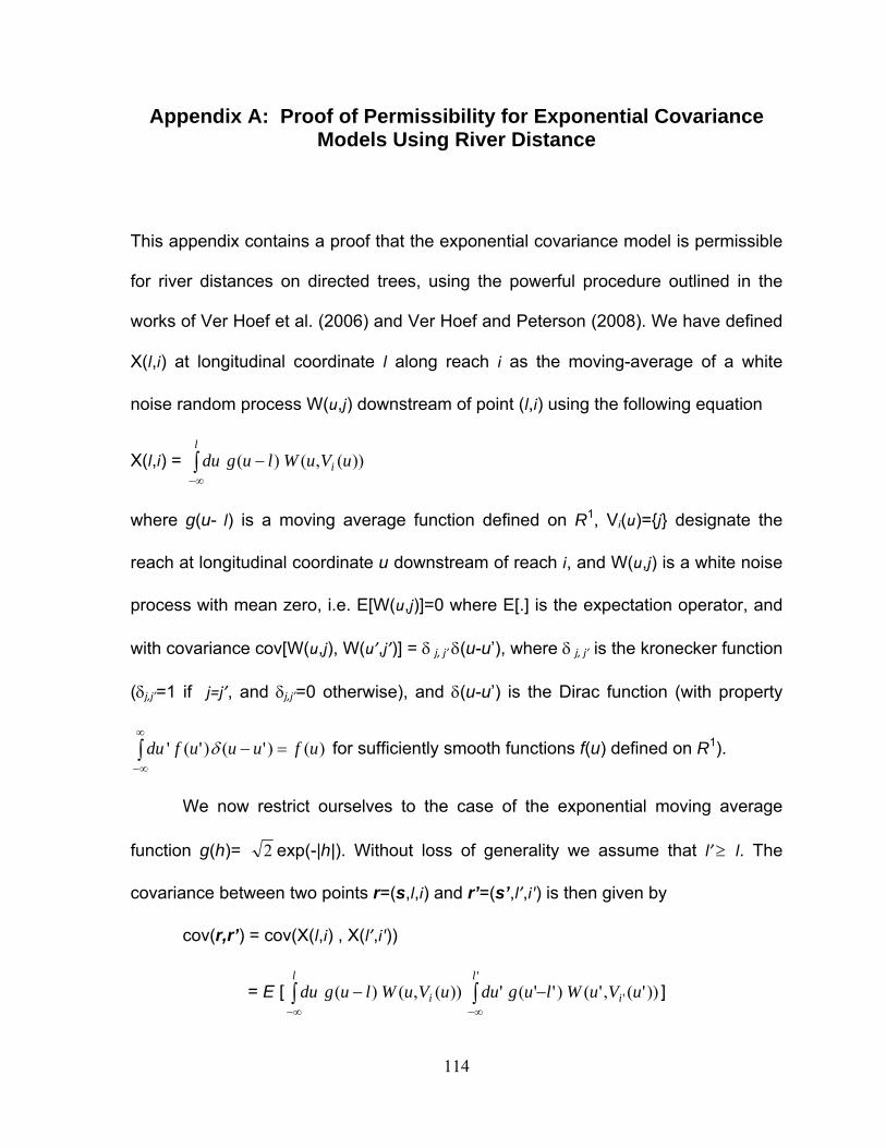
114
Appendix A: Proof of Permissibility for Exponential Covariance Models Using River Distance
This appendix contains a proof that the exponential covariance model is permissible
for river distances on directed trees, using the powerful procedure outlined in the
works of Ver Hoef et al. (2006) and Ver Hoef and Peterson (2008). We have defined
X(l,i) at longitudinal coordinate l along reach i as the moving-average of a white
noise random process W(u,j) downstream of point (l,i) using the following equation
X(l,i) =
l
i uVuWlugdu ))(,()(
where g(u- l) is a moving average function defined on R1, Vi(u)={j} designate the
reach at longitudinal coordinate u downstream of reach i, and W(u,j) is a white noise
process with mean zero, i.e. E[W(u,j)]=0 where E[.] is the expectation operator, and
with covariance cov[W(u,j), W(u’,j’)] = j, j’ (u-u’), where j, j’ is the kronecker function
(j,j’=1 if j=j’, and j,j’=0 otherwise), and (u-u’) is the Dirac function (with property
)()'()'(' ufuuufdu for sufficiently smooth functions f(u) defined on R1).
We now restrict ourselves to the case of the exponential moving average
function g(h)= 2 exp(-|h|). Without loss of generality we assume that l’ l. The
covariance between two points r=(s,l,i) and r’=(s’,l’,i') is then given by
cov(r,r’) = cov(X(l,i) , X(l’,i'))
= E [
l
i uVuWlugdu ))(,()(
'
' ))'(,'()''('l
i uVuWlugdu ]
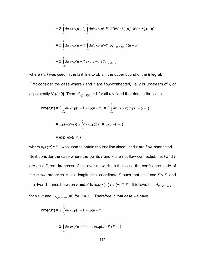
115
= 2
'
' ))]'(,'())(,([)''exp(')exp(l
ii
l
uVuWuVuWEluduludu
= 2
'
)'(),( )'()''exp(')exp('
l
uVuV
l
uuluduluduii
= 2 )(),( ')'exp()exp( uVuV
l
iiluludu
where l’ l was used in the last line to obtain the upper bound of the integral.
First consider the case where i and i’ are flow-connected, i.e. i' is upstream of i, or
equivalently Vi’(l)={i}. Then )(),( ' uVuV ii =1 for all u l and therefore in that case
cov(r,r’) = 2 )'exp()exp( luludul
= 2 ))'(exp()exp(0
llvvdv
= )2exp(2))'(exp(0
vdvll
= ))'(exp( ll
= exp(-dR(r,r’))
where dR(r,r’)= l’- l was used to obtain the last line since i and i’ are flow-connected.
Next consider the case where the points r and r’ are not flow-connected, i.e. i and i'
are on different branches of the river network. In that case the confluence node of
these two branches is at a longitudinal coordinate l” such that l” l and l” l’, and
the river distance between r and r’ is dR(r,r’)=( l- l”)+( l’- l”). It follows that )(),( ' uVuV ii =1
for u l” and )(),( ' uVuV ii =0 for l”<u l. Therefore in that case we have
cov(r,r’) = 2 )'exp()exp("
luludul
= 2 )'""exp()""exp("
lllullludul

116
= )"exp()"exp(2))"'()"(exp("
luludulllll
= exp(-dR(r,r’))
Hence we have shown that whether or not two points are flow-connected, their
covariance is exp(-dR(r,r’)). Since the covariance of the moving-average of a white
noise random process is a permissible covariance model (Ver Hoef et al., 2006),
then the exponential covariance is permissible with the river metric.

117
Appendix B: Mathematical Summary of Flow-weighted Covariance Models
The framework proposed in Ver Hoef et al (2006), and further used by
Cressie et al. (2006) and Ver Hoef and Peterson (2008) was a break-through to
obtain a large class of flow-weighted covariance models based on moving average
constructions. We refer the reader to their papers for an in-depth presentation of the
framework, but we provide here some mathematical steps using a slightly modified
notation that can then be compared with the alternate framework proposed by
Bernard-Michel and Fouquet (2006). Let’s define X(l,i) at longitudinal coordinate l
along reach i as the moving-average of a white noise random process W(u,j) on the
reaches upstream of point (l,i) using the following equation
X(l,i) =
l uVj
juWlugjidui
),()(),()(
where Vi(u) is the set of river reaches at longitudinal coordinate u upstream of reach
i, g(u- l) is a moving average function defined on R1, W(u,j) is a white noise process
with mean zero, and (i,j) is real number between 0 and 1 expressing the amount of
flow connection between reach i and j such that
)(
1),(uVj i
ji for u>l. The flow
connection between reach i and an upstream reach i' can be defined as the ratio
(i,i')=(i')/(i) where (i) is function that increases in the direction of flow. In that
case the property
)('
1)',(uVi l
ii u>l is verified if and only if (i) is a flow additive
function, i.e. such that if two reaches i’ and i" combine into reach i, then

118
(i')+(i")=(i). Flow discharges or watershed areas are physically meaningful
variables that can used to obtain (i) (see next section). The covariance between
two points r=(s,l,i) and r’=(s’,l’,i') is then given by
cov(r,r’) = cov(X(l,i) , X(l’,i'))
=E[
l uVj
juWlugjidui
),()(),()(
' )'(''
)','()''()','('l uVj
juWlugjidui
]
= ])','(),([)','(),()''(')(' )( )'(' '
l uVj uVjl
juWjuWEjijilugdulugdui i
=
' )( )'(''
', )'()','(),()''(')(l uVj uVj
jjl i i
uujijilugdulugdu
If r and r’ are not flow-connected, then )'(')( uVuV ii lu and '' lu , as a
result ', jj =0 )(uVj l and )'(' ' uVj l , so that the double summation is zero and
consequently cov(r,r’)=0. If r and r’ are flow-connected let us assume without loss of
generality that r is upstream of r’, i.e. l l’. Then using the property of the Dirac
function (
)()'()'(' ufuuufdu for sufficiently smooth functions f(u) defined on
R1) we obtain
cov(r,r’) =
l uVj uVjjj
i i
jijiluglugdu)( )(''
',)','(),()'()(
where l l’ was used in obtaining the lower bound of the integral. Since r and r’ are
flow-connected with r upstream of r’, it follows that )(')( uVuV ii lu , so that
the double summation reduces to a single summation as follow

119
cov(r,r’) =
l uVj i
jijiluglugdu)(
),'(),()'()(
Recall that (i', j)=(j)/(i'), (i, j)=(j)/(i) and
)(
1),(uVj i
ji for u>l, from which
we also get
)(
)()(uVj i
ij for u>l. Using these relationships it follows that
)',()'()(/)()'()(/)(),'(),()()(
iiiiiiijjijiuVjuVj ii
, which
when substituted in the equation above leads to
cov(r,r’) =
0
)'()()',( llvgvgduii
where the change of variable v=u‐l was used in the integral. Noting that dR(r,r’)=l‐l’
when r and r’ are flow-connected and l l’, and noting that (i,i')=0 when r and r’
are not flow-connected, then a permissible model for the covariance between r and
r’ (whether they are flow-connected or not) is given by
cov(r,r’) = )',( ii C1( dR(r,r’) )
where dR(r,r’)=|l‐l’| is the river distance between r and r’, and C1( . ) is the class of
permissible covariance functions in R1 defined by C1(h)=
0
)()( hvgvgdu for any
suitable moving average functions g(v). This class of permissible covariance
functions includes for example the strikingly beautiful Mariah (Ver Hoef, 2006)
model.
De Fouquet and Bernard-Michel (2006) proposed a framework that can be
used to expand the class of permissible flow-weighted covariance models. Along the

120
lines of the framework they proposed, let us here define X(l,i) at longitudinal
coordinate l along reach i as
X(l,i) =
)(
)(),(iVj
j lYji
where Vi(∞) is the set of flow-connected leaf reaches (i.e. sources) upstream of
reach i, (i,j) [0,1] quantifies the flow connection between reach i and its source j
such that
)(
1),(iVj
ji , and Yj(l) are independent zero mean random processes on
R1 with covariance cov(Yi(l),Yi(l’))=c1(h), h=|l‐l’|, where c1(h) may be any permissible
covariance function in R1 (i.e. such that it is the Fourier transform of a non-negative
bounded function in R1). The covariance between two points r=(s,l,i) and r’=(s’,l’,i')
is then given by
cov(r,r’) =
)( )('
)','(),('i iVj Vj
jiji cov(Yj(l),Yj’(l’))
If r and r’ are not flow-connected, then )(')( ii VV , as a result
cov(Yj(l),Yj’(l’))=0 )( iVj and )(' ' iVj , so that cov(r,r’)=0. If r and r’ are flow-
connected, assuming without loss of generality that r is upstream of r’, i.e. l l’, we
have
cov(r,r’) =
)(
1',)('
|)'(|)','(),('i iVj
jjVj
llcjiji
=
)(
1 |)'(|),'(),(iVj
llcjiji
= |)'(|)',( 1 llcii

121
Noting that (i,i')=0 when r and r’ are not flow-connected, we obtain that a
permissible model for the covariance between r and r’ (whether they are flow-
connected or not) is given by
cov(r,r’) = )',( ii c1( dR(r,r’) )
where c1( . ) can be any one dimensional permissible covariance function, which
includes the functions C1( . ) obtained with the moving average construction.

122
Appendix C: Flow-additive Functions
As described in Appendix B, the flow connection between reach i and an upstream
reach i’ can be defined as the ratio (i,i’)=(i’)/(i) where (i) is a flow additive
function, i.e. such that if two reaches i’ and i" combine into reach i, then
(i')+(i")=(i). We show here that the framework developed by Ver Hoef at al.
(2006) to quantify flow-connection provides a flexible method to construct the flow
additive function (i). Using their approach, let’s define the flow weight of a reach i’
as (i') such that if reaches i' and i" combine at a river junction, then (i')+(i")=1.
Using this variable, Ver Hoef at al. (2006) originally defined the flow connection
between reach i and an upstream reach i’ as (i,i’)= ',iiBj
j , where Bi,i’ is the set of
reaches in the flow-path Between reaches i and i’, exclusive of the downstream
reach i and inclusive of the upstream reach i'. This construction is equivalent to
defining the flow additive function as
(i)= iBj
j,1
,
where B1,i is the set of reaches in the flow-path between the river outlet (on a river
reach numbered 1 by convention) and reach i. Then it follows immediately that
(i,i’)=(i’)/(i)=
i
i
Bjj
Bjj
,1
',1
=
i
iii
Bjj
Bjj
Bjj
,1
',,1
=
',iiBjj ,
which, after taking its square-root, leads to the multiplier )',( ii = ',iiBj
j defined
in Ver Hoef et al. (2006) equation for flow-connected covariance models.

123
The weight of each combining reach can be calculated using a physically meaningful
parameter that increases in the direction of flow. Examples include watershed area,
discharge, cumulated river length, precipitation, pollution loading, etc. Let us denote
the value of this parameter at the downstream end of any reach i as Ai, and let ai be
the contribution within reach i, such that if reaches i’ and i" combine into reach i,
then Ai=Ai’+Ai”+ai. Using this parameter we can define the weights of combining
reaches i’ and i" as i’=Ai’/(Ai’+Ai”) and i"=Ai"/(Ai’+Ai”), respectively, which satisfies
i’+i"=1. The resulting flow additive function is then given by
(i)= iBj
j.1
=
iBj jCj
j
AA
A
.1 )(
=
iBj jDjD
j
aA
A
.1 )()(
where C(j) is the reach Combining with reach j, and D(j) is the reach immediately
Downstream of reaches j and C(j); so that AD(j)=Aj+AC(j)+aD(j). As can be seen in the
example of Fig. C1, the construction shown allows us to account for the contribution
of watershed area (or discharge, cumulated river length, etc.) within each reach.

124
Figure C1: Example of a river with 5 reaches, indicating for each reach i the contributing watershed area ai within reach i, the total watershed area Ai at the downstream end of reach i, and the corresponding flow additive function (i).
A simplified construction might consist in setting ai=1 for each leaf reaches, and
setting the contribution of non-leaf reaches to zero, i.e. aD(i)=0 i>1. In this case Ai
corresponds to the additive stream-order number used in Cressie et al. (2006), and
the flow additive function simplifies to (i)= Ai/A1. For illustration purposes, this
corresponds to setting a5=a4=a3=1 and a2=a1=0 in the example of Fig. C1, resulting in
the stream-order numbers A5=A4=A3=1, A2=2 and A1=3, and in the flow additive
function values (5)=1/3, (4)=1/3, (3)=1/3, (2)=2/3, (1)=1. This construction
provides a convenient way to obtain flow-connectivity if no information is available
Flow
11
2
22
5)5(aA
A
aA
A
a4
A4= a4
24)4(A
A
A
A
a2
A2= A4+A5+a2
2)2(
A
A
a3
A3= a3
3)3(A
A
a1
A1= A2+A3+a1
a5 A5= a5

125
about the contribution of watershed area (or discharge, cumulated river length, etc.)
within each reach.
Another simplification consists in weighting each reach equally, i.e. (i)=1/2 i>1,
which leads to (i)= iBj ,1
21 . This would correspond to using (5)=1/4, (4)=1/4,
(3)=1/2, (2)=1/2, (1)=1 in the example of Fig. C1, which is a slightly different
representation of flow-connectivity than that of based on stream-order number.

126
Appendix D: Movies Depicting Water Quality Trends Using river-BME
This appendix contains links to the animations of water quality for the case
studies in Chapters 4, 5, and 6. Each link will take you to a webpage where you can
view the movies in any web browser.
Chapter 4 Animations: Dissolved Oxygen
Movie 4.1 depicts monthly space/time trends of Dissolved Oxygen in the
Lower Delaware Basin, New Jersey: 2000-2005
http://www.unc.edu/depts/case/BMElab/studies/DO_NJ/RiverEstimate2000-2005_LowDel.gif
Movie 4.2 depicts monthly space/time trends of Dissolved Oxygen in the
Raritan Basin, New Jersey: 2000-2005
http://www.unc.edu/depts/case/BMElab/studies/DO_NJ/RiverEstimate2000-2005_Raritan.GIF
Chapter 5 Animations: Escherichia Coli
Movie 5.1 depicts daily space/time trends of E.coli in the Raritan Basin, New Jersey
for April and May, 2003.
http://www.unc.edu/depts/case/BMElab/studies/EC_NJ/Raritan_Ecoli_AprilMay2003.GIF

127
Chapter 6 Animations: Fish Tissue Mercury
Movie 6.1 depicts the biannual concentration of fish tissue mercury in the Cape Fear
and Lumber river basins, North Carolina: 1990-2004
http://www.unc.edu/depts/case/BMElab/studies/HgFish_NC/CapefearLumber_HgFish_2months.GIF

128
Works Cited
Adams, P.D., Hollabaugh, C.L., Harris, R.R. Environmental Assessment of the
Chattahoochee River in West Georgia: Relationships Between Flow and Sediment and Bacteria. Geological Society of America Annual Meeting. Denver, October 28-31, 2007.
Akita, Y., G. Carter, and M.L. Serre. 2007. Spatiotemporal non-attainment assessment of surface water tetrachloroethene in New Jersey, Journal of Environmental Quality, Vol. 36, no.2. Bailly, J-S, P. Monestiez, and P. Lagacherie. 2006. Modelling spatial variability
along drainage networks with geostatistics. Math. Geology, 38(5): 515-539. Bernard-Michel, C. and C. de Fouquet 2006. Construction of valid covariances along a hydrographic network. Application to specific water discharge on the Moselle Basin, in E. Pirard, A. Dassargues, and H.-B. Havenith, editors, Proceedings of IAMG'2006 - XIth International Congress for Mathematical Geology, Liège, Sep 3 - 8, CD S13_03, 4p, ISBN 978-2-9600644-0-7.
Balogh, S. J., Meyer, M. L. and Johnson, D. K. 1997, Mercury and suspended sediment loadings in the lower Minnesota River, Environ. Sci. Technol. Vol. 31, pp. 198–202.
BMElib: Bayesian Maximum Entropy Library for Space/Time Geostatistics. Version
2.0b for MATLAB. http://www.unc.edu/depts/case/BMELIB/ Bogaert, P. 1996. Comparison of kriging techniques in a space-time context. Math. Geology, Vol. 28, no.1, pp. 73-86. Chang, H. 2008. Spatial analysis of water quality trends in the Han River basin,
SouthKorea. Water Research 42: 3285-3304.
Chaplot V., Darboux F., Bourennane H., Leguedois S., Silvera N., Phachomphon K. 2006. Accuracy of interpolation techniques for the derivation of digital elevation models in relation to landform types and data density (2006) Geomorphology, Vol. 77, no.1-2, pp. 126-141.
Chen, Y., N. Belzile, and J. M. Gunn. 2001. Antagonistic effect of selenium on
mercury assimilation by fish populations near sudbury metal smelters? Limnology and Oceanography Vol. 46, no. 7, pp. 1814-1818.
Christakos G. 1990. A Bayesian/maximum-entropy view on the spatial estimation problem. Math. Geology, Vol. 22, no. 7, 763-776.

129
Christakos g. 1992. Random field models in Earth Sciences. Academic Press, San Diego. 474p. Christakos G. 2000. Modern spatiotemporal geostatistics. Oxford Univ. press, New York, 2nd edition (2001). Christakos, G. and X.Y. Li. 1998. Bayesian maximum entropy analysis and mapping:
A farewell to kriging estimators? Math. Geol. Vol. 30, pp. 435-462. Christakos, G. and M L. Serre. 2000. BME Analysis Of Particulate Matter
Distributions In North Carolina, Atmospheric Environment, Vol. 34, pp. 3393-3406.
Christakos G., P. Bogaert, and M.L. Serre. 2002. Temporal GIS: advanced functions for field-based applications. Springer, New York. 217p. Christakos, G., A. Kolovos, M.L. Serre, and F. Vukovich. 2004. Total ozone mapping by integrating data bases from remote sensing instruments and
empirical models, IEEE Trans. on Geosc. and Rem. Sensing, Vol. 42, no.5, pp. 991-1008.
Cope, W.G., Wiener, J.G., and Rada, R.G., 1990, Mercury accumulation in yellow perch in Wisconsin seepage lakes— Relation to lake characteristics: Environ. Tox. And Chem., no. 9, p. 931-940.
Coulliette, A.D., E.S. Money, M.L. Serre, R.T. Noble (2008) Space/Time Analyses of
Fecal Pollution and Rainfall in an eastern North Carolina Estuary, Environmental Science & Technology, submitted.
Cressie, N. The Origins of Kriging. Math. Geol. 1990. Vol. 22, No.3, p 239-252.
Cressie, N.A.C. 1993. Statistics for spatial data: John Wiley & Sons, New York, rev. ed., 900p. Cressie, N., J. Frey, B. Harch, M.Smith. 2006. Spatial Prediction on a River
Network. Journal of Agricultural Biological And Environmental Statistics, Vol. 11, no.2, pp.127-150.
Curriero, F. C. 2006. On the use of non-Euclidean distance measures in
geostatistics. Math. Geology Vol. 38, no.8, pp. 907-925. Darwish, Kh. M., Kotb M.M., Ali R. Mapping Soil Salinity Using Collocated Cokriging
in Bayariya, Oasis, Egypt. Proceedings of the 5th International Symposium on Spatial Data Quality. ITC Enschede, The Netherlands. June 13-15, 2007.
Delhomme, J.P. Kriging in the Hydrosciences. Advances in Water Res. 1978. Vol.

130
1, No.5, p 251-266. Dirks K.N., Hay J.E., Stow C.D., Harris D. High-resolution studies of rainfall on
Norfolk Island Part II: Interpolation of rainfall data (1998) Journal of Hydrology, Vol. 208, no. 3-4, pp. 187-193.
Dorner, S.M., Anderson W.B., Huck, P.M., Gaulin T., Candon H.L., Slawson R.M.,
Payment, P. Pathogen and Indicator Variability in a Heavily Impacted Watershed. Journal of Water & Health. 2007. Vol. 5, No.2; p 241-257.
FDA, 2001 Food and Drug Administration (FDA). 2001. FDA consumer advisory.
Available:http//www.fda.gov/bbs/topics/ANSWERS/2000/advisory.html. Fuentes, M. 2004. Testing for separability of spatiotemporal covariance functions. Journal of Statistical Planning and Inference. 136(2):447-466. Fulkerson M, FN Nnadi. 2006. Predicting mercury wet deposition in Florida: A
simple approach. Atmos. Environ. Vol. 40, no. 21, pp. 3962-3968. Goovaerts, P. Geostatistics for Natural Resources Evaluation. Oxford University
Press: London. 1997. Gordon, Nancy D.; Thomas A. McMahon; Christopher J. Gippel; Rory J. Nathan.
2004. Stream Hydrology:an Introduction for Ecologists:Second Edition. John Wiley and Sons: pp. 183-184
Grieb, T.M., Driscoll C.T., Gloss S.P., Shofield C.S., Bowie G.L., Porcella D.B.
1990. Factors affecting mercury accumulation in fish in the upper Michigan peninsula. Environ. Tox. And Chem. Vol. 9, pp. 919-930.
Griffith, J.F., Aumand, L.A., Lee, I.M., Mcgee C.D., Othman, L.L., Ritter, K.J.,
Walker, O.K., Weisberg, S.B. Comparison and Verification of Bacterial Water Quality Indicator Measurement Methods Using Ambient Coastal Water Samples. Environ. Modeling and Assessment. Vol. 116, p 335-344.
Hearn, P.P., Wente, S.P., Donato, D.I., and Aguinaldo, J.J., 2006, "EMMMA: A web-
based system for environmental mercury mapping, modeling, and analysis", U.S. Geological Survey Open File Report 2006-1086, 13p.
Huckabee, J.W., Elwood, J.W., and Hildebrand, S.G., 1979, Accumulation of
mercury in freshwater biota, in Nriagu, J.O., ed., Biogeochemistry of Mercury in the Environment: Elsevier/North-Holland Biomedical Press, New York, pp. 277-302.

131
Jager, H. I., Sale, M.J., Schmoyer, R.L. 1990. Cokriging to Assess Regional Stream Quality in the Southern Blue Ridge Province. Water Resources Res. Vol. 26, No. 7, p 1401-1412.
Julien, P.Y. River Mechanics. Cambridge University Press, 40 W. 20th St., New
York, NY 10011-4211. 434 pp. 2002. ISBN 0-521-56284-8 Kannan K, RG Smith Jr., RF Lee, HL Windom, PT Heitmuller, JM Macauley, JK
Summers. 1998. Distiribution of total mercury and methylmercury in water, sediment, and fish from south florida estuaries. Archives of Environmental Contamination and Toxicology. Vol. 34, no.2, pp.109-118.
King, R.S., M.E. Baker, D.F. Whigham, D.E. Weller, T.E. Jordan, P.F. Kazyak, and
M.K. Hurd. 2005. Spatial considerations for linking watershed land cover to ecological indicators in streams. Ecological Applications, Vol. 15, pp. 137-153.
Kolovos, A., G. Christakos, D.T. Hristopulos, and M.L. Serre. 2004. Methods for generating non-separable spatiotemporal covariance models with potential environmental applications, Advances in Water Resources. Vol. 27, no.8, pp. 815-830. Kravchenko, A. N. 2003. Influence of Spatial Structure on Accuracy of Interpolation
Methods Soil Sci Soc Am J 67: pp. 1564-1571 Kyriakidis, P.C. and A.G. Journel. 1999. Geostatistical space-time models: a review. Math. Geology. Vol. 31, no. 6, pp. 651-684. Lange, T. R., H. E. Royals, and L. L. Connor. 1993. Influence of water chemistry on
mercury concentration in largemouth bass from Florida lakes. Transactions of the American Fisheries Society. Vol. 122, pp. 74-84.
Law D.C.G., M.L. Serre, G . Christakos, P.A. Leone, W.C. Miller. 2004. Spatial analysis and mapping of sexually transmitted diseases to optimize intervention and prevention strategies, Sexually Transmitted Infections, Vol. 80, pp. 294-299. Law, D.C.G., K. Bernstein, M.L. Serre, C.M. Schumacher, P.A. Leone, J.M. Zenilman, W.C. Miller, and A.M. Rompalo. 2006. Modeling an early syphilis outbreak through space and time using the bayesian maximum entropy approach, Annals of Epidemiology, Vol. 16, no.11, pp. 797-804. Lee, S.J. (2005) Models of Soft Data in Geostatistics and Their Application in
Environmental and Health Mapping, Ph.D. Dissertation, Dept. of

132
Environmental Sciences and Engineering, University of North Carolina at Chapel Hill, NC, USA.
Li Z., Zhang Y-K., Schilling K., Skopec M. Cokriging Estimation of Daily Suspended
Sediment Loads. Journal of Hydro. 2006. Vol. 327, p 389-398. LoBuglio, J.N., G.W. Characklis, M.L. Serre. 2007. Cost-effective water quality
assessment through the integration of monitoring data and modeling results, Water Resources Research. 2007. 43, W03435, doi:10.1029/2006WR005020
Lopes, T.J., and Bender, D.A., 1998 , Nonpoint sources of volatile organic
compounds in urban areas, in Source Water Assessment and Protection--A Technical Conference, Dallas, Tex., April 28-30, 1998 [Proceedings]: Fountain Valley, National Water Research Institute, p. 199-200.
MacCrimmon, H.R., Wren, C.D., and Gots, B.L., 1983, Mercury uptake by lake trout,
Salvelinus namaycush, relative to age growth, and diet in Tadenac Lake with comparative data from other Precambrian Shield Lakes: Canadian Journal of Fisheries and Aquatic Sciences, no. 40, p. 114-120.
Mallin, M.A., K.E. Willams, E.C. Esham, and R.P. Lowe. 2000. Effect of Human
Development on Bacteriological Water Quality in Coastal Watersheds. Ecological Applications. Vol. 10, No. 4, 1047-1056.
Mason, R.P., Lawson, N.M., and Sullivan, K.A. 1997. Atmospheric deposition to
the Chesapeake Bay watershed-regional and local sources. Atmos. Environ., Vol. 31, No. 23, pp. 2531-3540.
Miller D.R., and Akagi H. 1979. pH affects mercury distribution, not methylation.
Ecotoxicol Environ Saf. Vol. 3, no.1, pp. 36-38. Money, E., Carter G.P., Serre, M.L. Using River Distance in the space/time
estimation of dissolved oxygen along two impaired river networks in New Jersey. Water Research. Accepted subject to minor revisions.
Money, E., Carter G.P., Serre, M.L. Covariance models for directed tree river
networks, UNC-BMElab Technical Report 2008-08, Department of Environmental Sciences and Engineering, University of North Carolina, Chapel Hill, NC, USA. 2008. 18p.
Morel F.M.M., Kraepiel A.M.L., Amyot M. 1998. The chemical cycle and
bioaccumulation of mercury. Annual Review of Ecology and Systematics. Vol. 29, pp. 543-566.

133
Moran, M.J., Rick M. Clawges, and John S. Zogorski, 2002 , Methyl tert-butyl ether in ground and surface water of the United States, inDiaz, A.F., and Drogos, D.L., eds., Oxygenates in Gasoline(Symposium Series 799): Washington, D.C., American Chemical Society, p. 2-16.
NHD. 2008. National Hydrography Dataset. http://nhd.usgs.gov National Research Council. 2000. Toxicological effects of methylmercury.
Committee on the Toxicological Effects of methylmercury, Board on Environmental Studies and Toxicology, Commission on Life Sciences. National Academy Press, Washington D.C.
NJDEP (New Jersey Dept. of Environmental Protection). 2002. Raritan Basin:
Portrait of a Watershed. Raritan Basin Watershed Project, New Jersey Water Supply Authority, Watershed Management Programs. New Jersey Dept. of Environmental Protection.
NJDEP. 2006a. Surface Water Quality Standards. Title 7, New Jersey Administrative Code. N.J.A.C. 7:9B. NJDEP. 2006b. New Jersey 2006 integrated water quality monitoring and
assessment report. Water Monitoring and Standards, New Jersey Dept. Of Env. Protection.
NCDENR (North Carolina Department of Environment and Natural Resources).
2004. Cape Fear Basinwide Assessment. Basinwide Assessment Report. Division of Water Quality, Environmental Sciences Section.
NCDENR. 2006. North Carolina Water Quality Assessment and Impaired Waters
List (2006 Integrated 303(d) and 303(b) reports). NCDENR Division of Water Quality, Planning Section.
NCDENR. 2007. Lumber River Basinwide Assessment. Basinwide Assessment
Report. North Carolina Department of Environment and Natural Resources, Division of Water Quality, Environmental Sciences Section.
NCDWQ (North Carolina Division of Water Quality). 2004. 2002/2003 Eastern
Regional Mercury Study summary. Modeling/TMDL Unit. NCDWQ. 2006. Eastern Regional Mercury Study Extension Report.
Modeling/TMDL Unit. Noble, R.T., Weisberg, S.B., Leekaster, M.K., Mcgee, C.D., Ritter, K., Walker, K.O.,

134
Vainik, P.M. Comparison of Beach Water Quality Indicator Measurement Methods. Environ. Modeling and Assessment. 2003. Vol. 81, p 301-312.
Peterson SA, JV Sickle. 2007. Mercury concentration in fish from streams and
rivers throughout the western United States. Environmental Science & Technology, Vol. 41, no.1, pp. 58-65.
Peterson E.E., Merton A.A., Theobald D.M. & Urquhart N.S. 2006. Patterns in
spatial autocorrelation in stream water chemistry. Environmental Monitoring and Assessment Vol. 121, pp. 569-594.
Peterson, E.E., and N.S. Urquhart. 2006. Predicting water quality impaired stream segments using landscape-scale data and a regional geostatistical
model: a case study in Maryland. Environmental Monitoring and Assessment, Vol. 121, pp. 613-636. Peterson, E.E., Theobold D. & Ver Hoef, J.M. 2007. Geostatistical modeling on
stream networks: developing valid covariance matrices based on hydrologic distance and stream flow. Freshwater Biology Vol. 52, pp. 267-279.
Porcella, D.B., 1995, Aquatic biogeochemistry and mercury cycling model (MCM), in National Forum on Mercury in Fish Proceedings, U.S. Environmental Protection Agency, Office of Water, EPA 823-R-95-002, 211p.
Rasmussen, T.J., A.C. Ziegler, P.P. Rasmussen. 2005. Estimation of constituent concentrations, densities, loads, and yields in lower Kansas River, northeast Kansas, using regression models and continuous water-
quality monitoring, January 2000 through December 2003. USGS Scientific Investigation Reports: 2005-5165. 126p. Reeves, R.L., Grant, S.B., Mrse, R.D., Oancea, C.M.C., Sanders, B.F., Bochm, A.B.
2004. Scaling and Management of fecal indicator bacteria in runoff from coastal urban watershed in southern California. Environ. Sci. Technol. Vol. 38, pp 2637-2648.
Reis A.H. Constructal view of scaling laws of river basins.
2006. Geomorphology, Vol. 78, no. 3-4, pp. 201-206. Rose J., Hutcheson M.S., West C.W., Pancorbo O., Hulme K., Cooperman A.,
DeCesare G., Isaac R., Screpetis A. 1999. Fish mercury distribution in Massachusetts, USA lakes. Environ. Tox. And Chem. Vol. 18, No. 7, pp. 1370-1379.
Sackett, D.K., D.D. Aday, J.A. Rice, W.G. Cope. 2008. A state-wide assessment of
mercury dynamics in North Carolina waterbodies and fish. In review.

135
Savelieva, E., V. Demyanov, M. Kanevski, M.L. Serre, and G. Christakos. 2005. BME-Based Uncertainty Assessment of the Chernobyl Fallout, Geoderma, Vol. 128, pp. 312-324.
Sayler, G.S., Nelson J.D., Justice A., Colwell R.R. 1975. Distribution and
Significance of Fecal Indicator Organisms in the upper Chesapeake Bay. Applied Micro. Vol. 30, pp. 625-638.
Seo, D.J., Krajewski, W.F., Azimi-Zonooz, A., Bowles, D.S. 1990. Stochastic
Interpolation of Rainfall Data from Rain Gauges and Radar Using Cokriging. Water Resources Res. Vol. 26, No. 5, pp. 915-924.
Serre M.L., P. Bogaert, G. Christakos. 1998. Computational investigations of Bayesian maximum entropy spatiotemporal mapping. In: Buccianti A,
Nardi G., Potenza R (eds) IAMG98, Proceed. Of 4th Annual Conference of the International Association for Mathematical Geology 1:117-122, De Frede Editore, Naples, Italy. Serre, M. L., and G. Christakos. 1999. Modern geostatistics: computational BME in the light of uncertain physical knowledge--the equus beds study, Stochastic Environmental Research and Risk Assessment, Vol. 13, no.1, pp.
1-26. Serre, M.L., G. Carter, and E. Money. 2004. Geostatistical space/time estimation of water quality along the raritan river basin in New Jersey, in C.T. Miller, M.W. Farthing, W.G. Gray, and G.F. Pinder, editors, Computational Methods in Water Resources 2004 International Conference, Elsevier, 2:1839-1852. Serre, M.L, and S.J. Lee (2006) Risk Mapping of Subsurface Arsenic in New
England using Measurement Error Model and Secondary Soil-pH Data, Eric Pirard et. al., editors, Proceedings of IAMG 2006-XIth International Congress for Mathematical Geology, ISBN 978-2-9600644-0-7.
Song, S.S., Warren-Hick J., Keating D., Moore R.J., Teed R.S. 2001. A predictive
model of mercury fish tissue concentrations for the southeastern United States. Environ. Sci. Technol., Vol 35, no. 5, pp. 941-947.
Southworth, G.R., Peterson M.J., Bogle M.A. 2004. Bioaccumulation factors for
mercury in stream fish. Environmental Practice. Vol. 6, pp. 135-143. Stein, M. 1986. A simple model for spatial-temporal processes. Water Resources Research. Vol. 22, no. 13, pp. 2107-2110. Stein, M.L. 1999. Interpolation of Spatial Data: Some Theory for Kriging, Springer,
New York, 247p.
136
Strahler, A. N. 1952. Hypsometric (area altitude) analysis of erosional topology.
Geological Society of America Bulletin, 63, 1117 - 1142. Sullivan KA, RP Mason. 1998. The concentration and distribution of Mercury in
the Lake Michigan. The Science of the Total Environment, Vol. 213, no. 1, pp. 213-228.
Tortorelli, R.L. and B.E. Pickup. 2006. Phosphorus concentrations, loads, and yields in the Illinois River basin, Arkansas and Oklahoma, 2000–2004. USGS Scientific Investigation Reports: 2006-5175, 38p. Ullrich, S. M., T. W. Tanton, and S.A. Abdrashitova. 2001. Mercury in the aquatic
environment: A review of factors affecting methylation. Critical reviews in environmental science and technology ,Vol. 31, no.3, pp. 241-293.
USEPA (United States Environmental Protection Agency). 1997a. Mercury study
report to congress Vol. VII: Characterization of human health and wildlife risks from mercury exposure in the United States. Air Quality Planning and Standards, Research, and Development, USEPA, EPA-452/R-97-009, Washington, DC.
USEPA (United States Environmental Protection Agency). 2000. Guide to
Monitoring Water Quality. Section 5.11 Fecal Bacteria.
USEPA (United States Environmental Protection Agency). 2001. Notice of availability of water quality criterion for the protection of human health: methylmercury. Federal Register Vol. 66, no. 5, pp. 1334-1359.
USEPA (United States Environmental Protection Agency). 2007. 2005/2006
National listing of fish advisories. Office of Water. USEPA. EPA-823-F-07-003, Washington, DC.
Ver Hoef, J.M., Peterson E.E., Theobold D. 2006. Spatial statistical models that
use flow and stream distance. Environmental and Ecological Statistics 13: 449-464.
Ver Hoef, J.M., Peterson E.E. Submitted in 2008. A moving average approach for spatial statistical models of stream networks, Journal American Statistical Association. Accepted subject to minor revisions.
Vidon, P., Tedesco, L.P., Wilson, J., Campbell M.A., Casey L.R. Direct and Indirect
Hydrological Controls on E.coli Concentration and Loading in Midwestern Streams. Journal of Env. Qual. 2008. Vol. 37, pp. 1761-1768.
Water on the Web. 2004. Understanding Water Quality Parameters: Dissolved

137
Oxygen. http://waterontheweb.org/under/waterquality/oxygen.html accessed on Feb. 24, 2007. Watras CJ, RC Back, S Halvorsen, RJ Hudson, KA Morrison, SP Wente. 1998.
Bioaccumulation of mercury in pelagic freshwater food webs. Sci Total Environ. Vol. 219, No.2-3, pp. 183-208.
Wente, S.P., 2004, "A statistical model and national data set for partitioning fish-
tissue mercury concentration variation between spatiotemporal and sample characteristic effects", U.S. Geological Survey Scientific Investigation Report 2004-5199, 15p.
Wiener, J.G., and Spry, D.J., 1996, Toxicological significance of mercury in
freshwater fish, in Beyer, W.N., Heinz, G.H., and Redmon-Norwood, A.W., eds., Environmental Contaminants in Wildlife—Interpreting Tissue Concentrations: Lewis Publ., Boca Raton, Fla., p. 297-339.
Williams, L.K. 2006. Health effects of methylmercury and North Carolina’s advice
on eating fish. North Carolina Dept. of Health and Human Services. Occupational and Environmental Epidemiology Branch.
Wilson, S., M.L. Serre. 2007. Examination of atmospheric ammonia levels near hog CAFOs, homes, and schools in eastern NC. Atmospheric Environment, Vol. 41, no. 23, pp. 4977-4987. Winfrey, M.R., and Rudd, J.W.M. 1990. Environmental factors affecting the
formation of methylmercury in low pH lakes. Environ. Tox. And Chem. Vol. 9, no. 7, pp. 853-869.