Embed Size (px)
Citation preview
Modern Spectral and Physical Interference Correction in Inductively Coupled Plasma Optical Spectroscopy
Christine Rivera
Product Specialist
Agilent Technologies
Page 1 1
ICP-OES Quantitative Analysis - a Relative Technique
Standards solutions prepared with a known concentration are required to quantitatively relate measured response of the element in the working standard to the measured response of an element in a test solution.
The assumption:
• Measured working standard response for each element is related to the response of the element measured in the test solution which correlates to the concentration of the element in the test solution.
The assumption is only true when the standard solution and test solution are identical (mineral content, viscosity, polyatomic structures).
• Frequently, this is not the case.
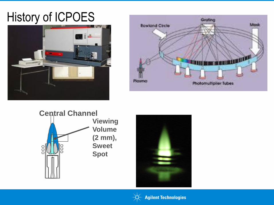
History of ICPOES
Viewing
Volume
(2 mm),
Sweet
Spot
Central Channel
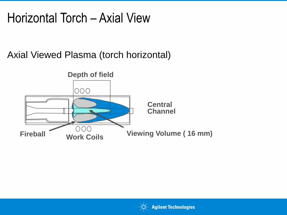
Horizontal Torch – Axial View
Axial Viewed Plasma (torch horizontal)
Depth of field
Viewing Volume ( 16 mm)
CentralChannel
Fireball Work Coils
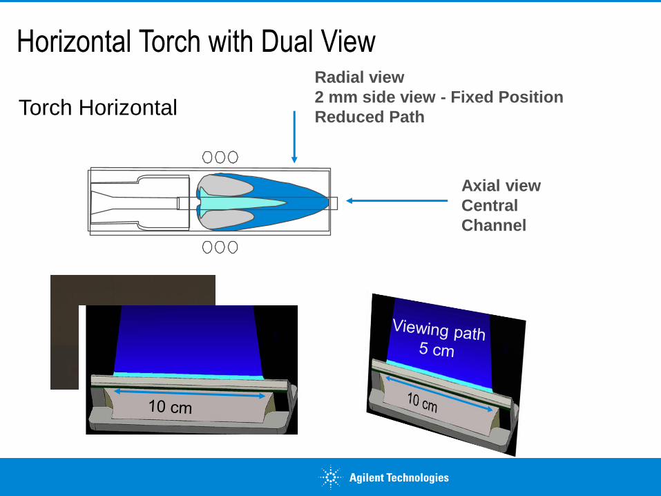
Horizontal Torch with Dual View
Torch Horizontal
Axial view
Central
Channel
Radial view
2 mm side view - Fixed Position
Reduced Path

Wavelength Separation
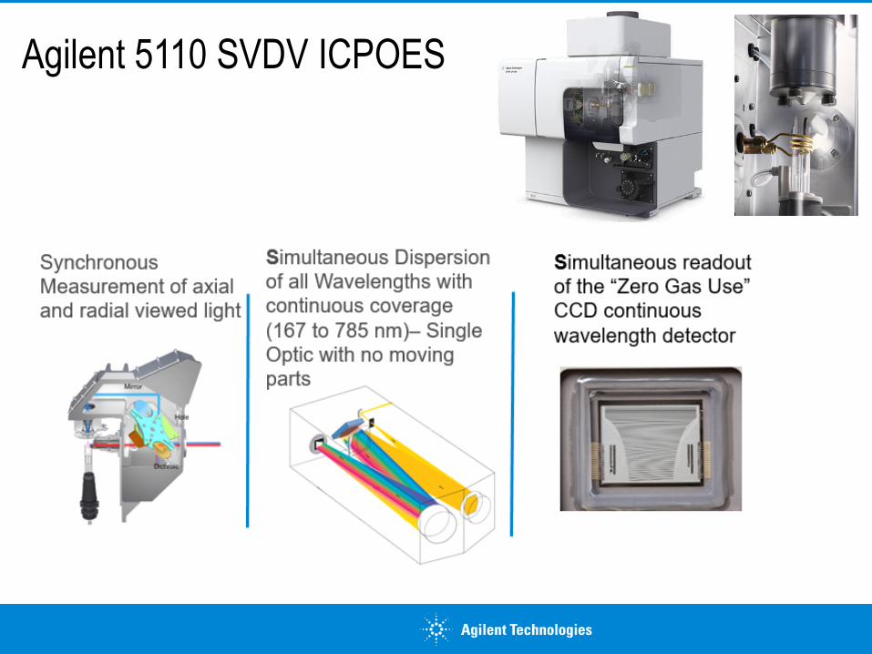
Agilent 5110 SVDV ICPOES
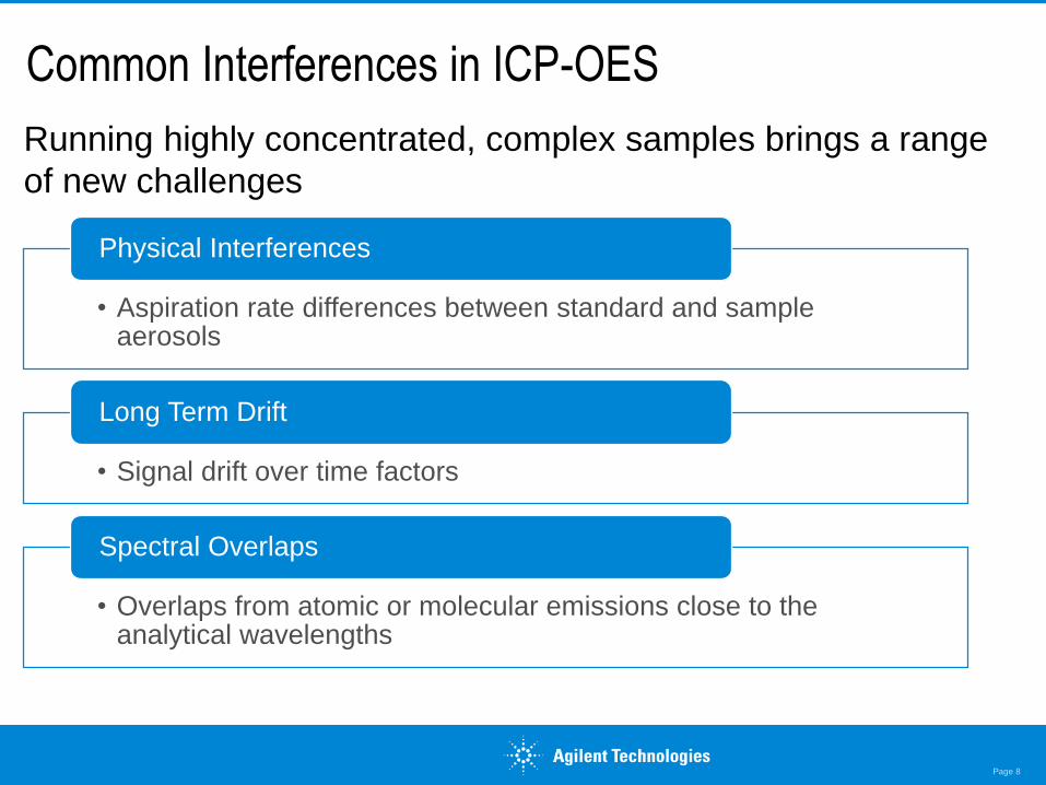
Common Interferences in ICP-OES
Running highly concentrated, complex samples brings a range
of new challenges
Page 8
• Aspiration rate differences between standard and sample aerosols
Physical Interferences
• Signal drift over time factors
Long Term Drift
• Overlaps from atomic or molecular emissions close to the analytical wavelengths
Spectral Overlaps
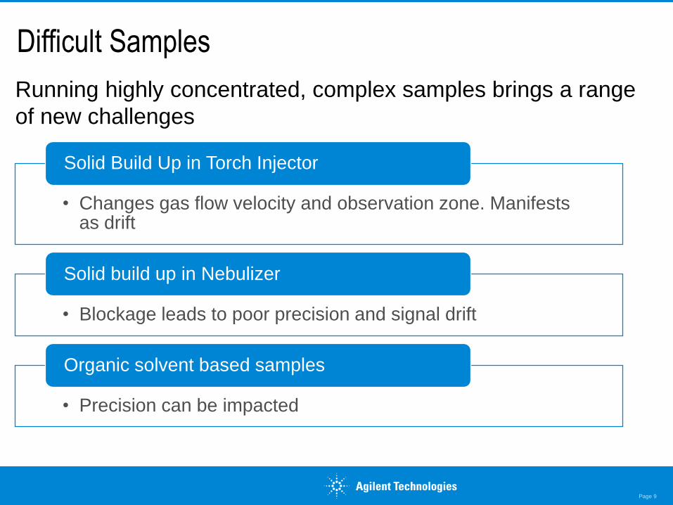
Difficult Samples
Running highly concentrated, complex samples brings a range
of new challenges
Page 9
• Changes gas flow velocity and observation zone. Manifests as drift
Solid Build Up in Torch Injector
• Blockage leads to poor precision and signal drift
Solid build up in Nebulizer
• Precision can be impacted
Organic solvent based samples
Physical Interferences – Particle Blockage
Blockage of sample introduction system• Results from high levels of particles in samples
- Blockage can be partial or can be full.
Blockage results in:• Suppressed emission response compared to standard response
- Short and long term drift.
• Enhanced emission response compared to standard response
- Partial blockage reduces solvent to the plasma which can increase response for elements which require hot plasma conditions for ionization.
• Poor precision (% RSD)
• Not always easy to detect
- Requires microscopic examination of the sample introduction system.
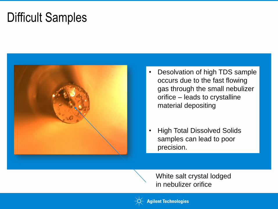
Difficult Samples
• Desolvation of high TDS sample
occurs due to the fast flowing
gas through the small nebulizer
orifice – leads to crystalline
material depositing
• High Total Dissolved Solids
samples can lead to poor
precision.
White salt crystal lodged
in nebulizer orifice
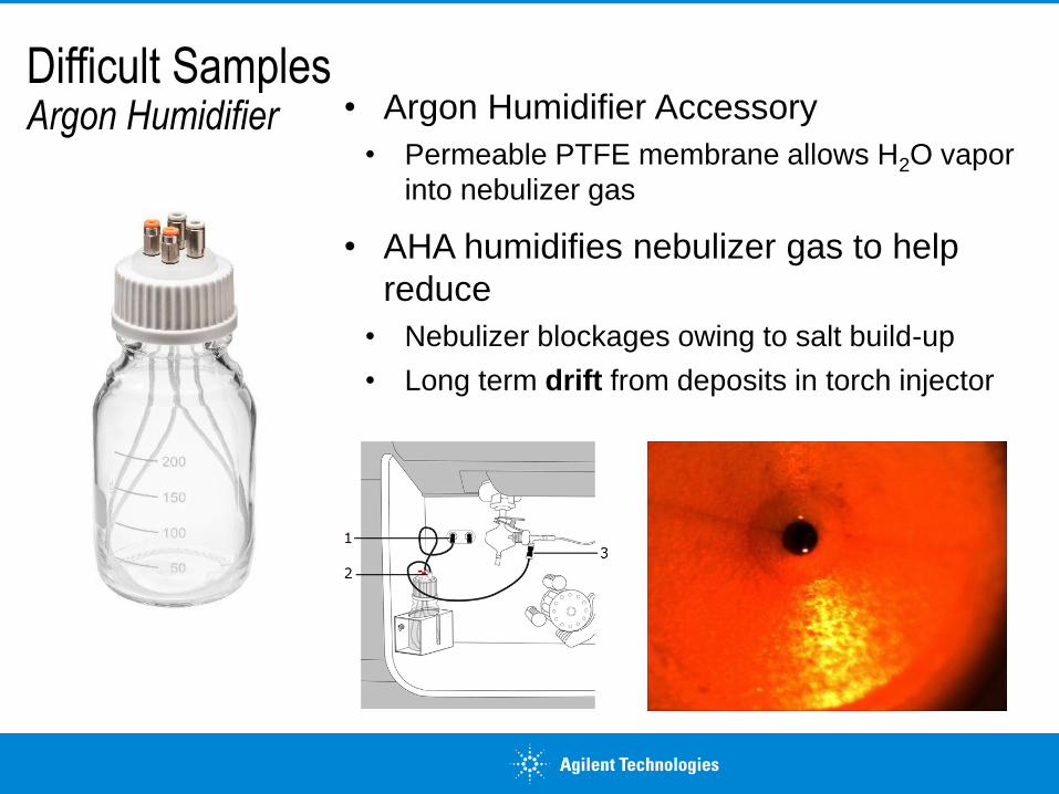
Difficult Samples Argon Humidifier • Argon Humidifier Accessory
• Permeable PTFE membrane allows H2O vapor
into nebulizer gas
• AHA humidifies nebulizer gas to help
reduce
• Nebulizer blockages owing to salt build-up
• Long term drift from deposits in torch injector
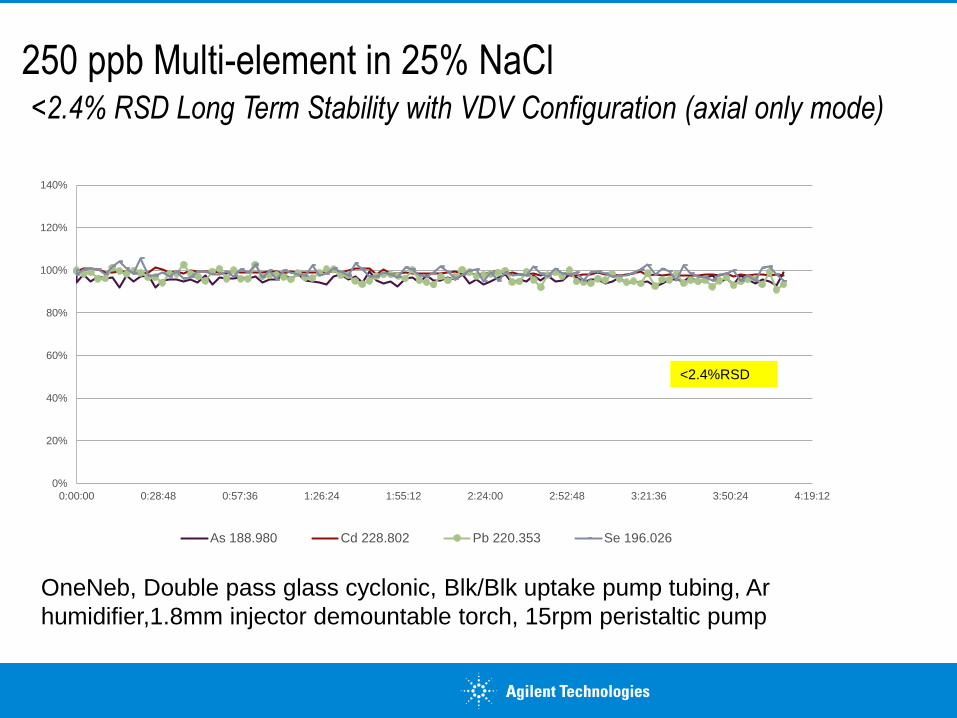
250 ppb Multi-element in 25% NaCl<2.4% RSD Long Term Stability with VDV Configuration (axial only mode)
0%
20%
40%
60%
80%
100%
120%
140%
0:00:00 0:28:48 0:57:36 1:26:24 1:55:12 2:24:00 2:52:48 3:21:36 3:50:24 4:19:12
As 188.980 Cd 228.802 Pb 220.353 Se 196.026
<2.4%RSD
OneNeb, Double pass glass cyclonic, Blk/Blk uptake pump tubing, Ar
humidifier,1.8mm injector demountable torch, 15rpm peristaltic pump
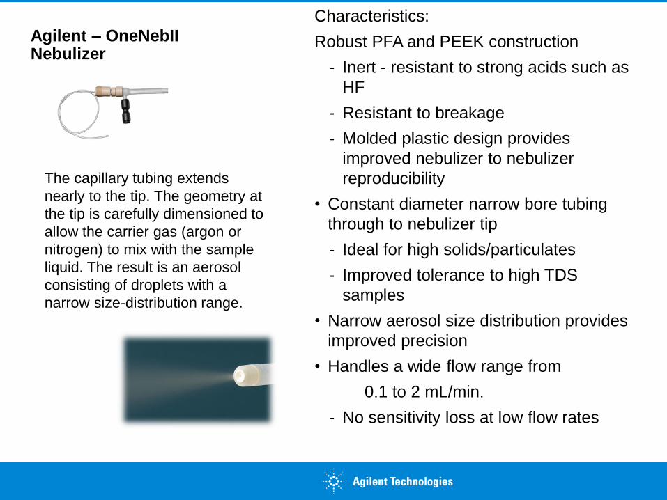
Agilent – OneNebIINebulizer
The capillary tubing extends
nearly to the tip. The geometry at
the tip is carefully dimensioned to
allow the carrier gas (argon or
nitrogen) to mix with the sample
liquid. The result is an aerosol
consisting of droplets with a
narrow size-distribution range.
Characteristics:
Robust PFA and PEEK construction
- Inert - resistant to strong acids such as
HF
- Resistant to breakage
- Molded plastic design provides
improved nebulizer to nebulizer
reproducibility
• Constant diameter narrow bore tubing
through to nebulizer tip
- Ideal for high solids/particulates
- Improved tolerance to high TDS
samples
• Narrow aerosol size distribution provides
improved precision
• Handles a wide flow range from
0.1 to 2 mL/min.
- No sensitivity loss at low flow rates
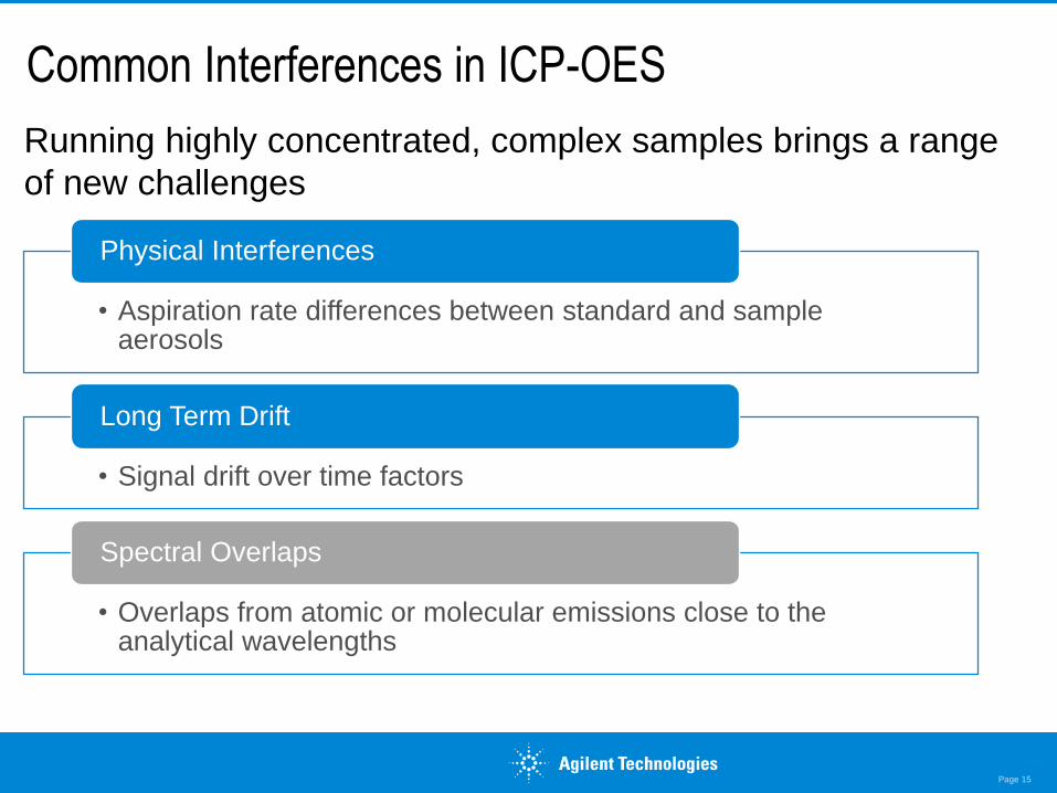
Common Interferences in ICP-OES
Running highly concentrated, complex samples brings a range
of new challenges
Page 15
• Aspiration rate differences between standard and sample aerosols
Physical Interferences
• Signal drift over time factors
Long Term Drift
• Overlaps from atomic or molecular emissions close to the analytical wavelengths
Spectral Overlaps
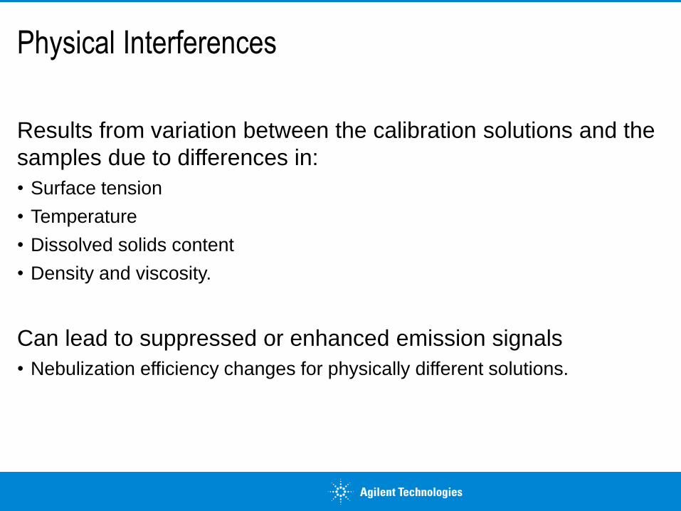
Physical Interferences
Results from variation between the calibration solutions and the
samples due to differences in:
• Surface tension
• Temperature
• Dissolved solids content
• Density and viscosity.
Can lead to suppressed or enhanced emission signals
• Nebulization efficiency changes for physically different solutions.
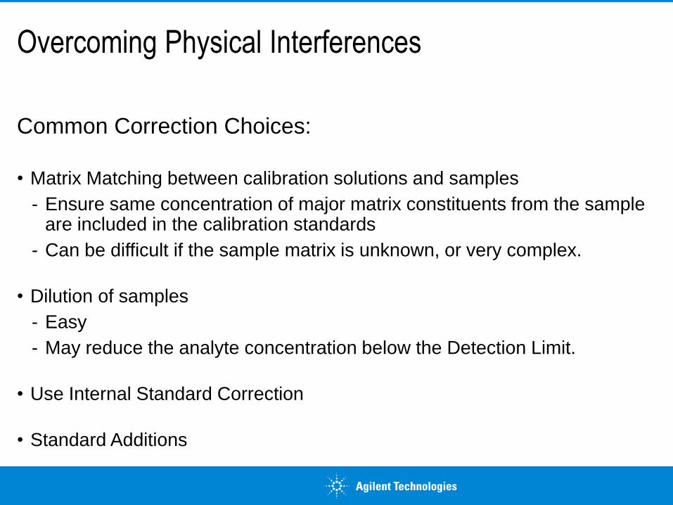
Overcoming Physical Interferences
Common Correction Choices:
• Matrix Matching between calibration solutions and samples
- Ensure same concentration of major matrix constituents from the sample are included in the calibration standards
- Can be difficult if the sample matrix is unknown, or very complex.
• Dilution of samples
- Easy
- May reduce the analyte concentration below the Detection Limit.
• Use Internal Standard Correction
• Standard Additions
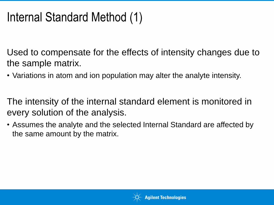
Internal Standard Method (1)
Used to compensate for the effects of intensity changes due to
the sample matrix.
• Variations in atom and ion population may alter the analyte intensity.
The intensity of the internal standard element is monitored in
every solution of the analysis.
• Assumes the analyte and the selected Internal Standard are affected by
the same amount by the matrix.
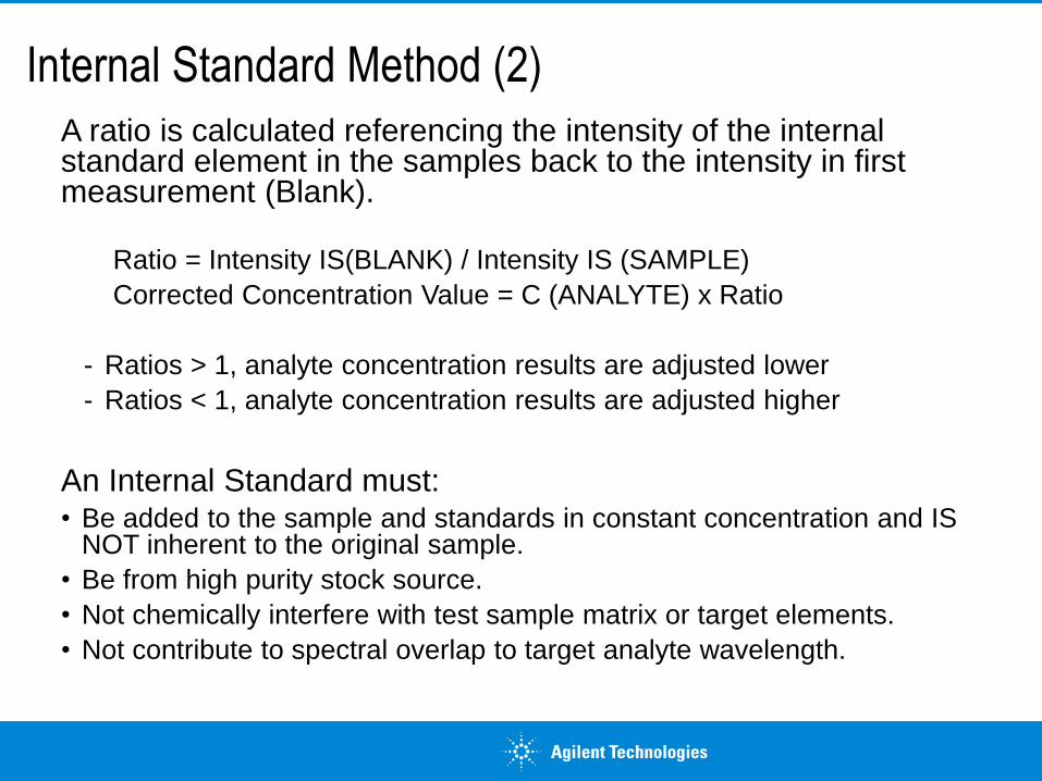
Internal Standard Method (2)
A ratio is calculated referencing the intensity of the internal standard element in the samples back to the intensity in first measurement (Blank).
Ratio = Intensity IS(BLANK) / Intensity IS (SAMPLE)
Corrected Concentration Value = C (ANALYTE) x Ratio
- Ratios > 1, analyte concentration results are adjusted lower
- Ratios < 1, analyte concentration results are adjusted higher
An Internal Standard must:• Be added to the sample and standards in constant concentration and IS
NOT inherent to the original sample.
• Be from high purity stock source.
• Not chemically interfere with test sample matrix or target elements.
• Not contribute to spectral overlap to target analyte wavelength.
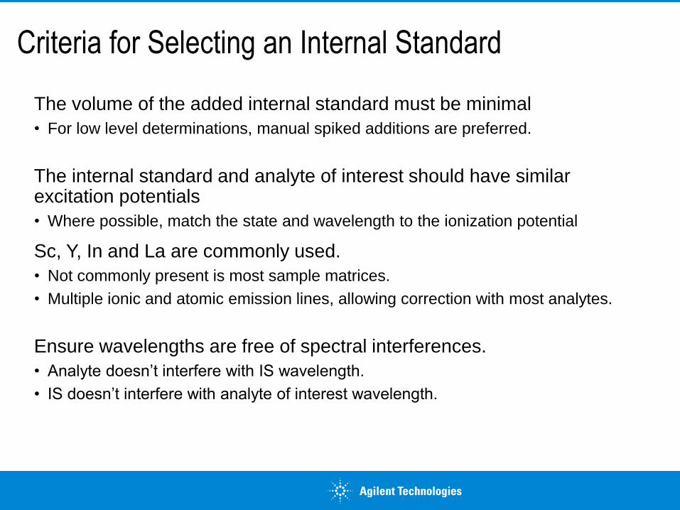
Criteria for Selecting an Internal Standard
The volume of the added internal standard must be minimal
• For low level determinations, manual spiked additions are preferred.
The internal standard and analyte of interest should have similar excitation potentials
• Where possible, match the state and wavelength to the ionization potential
Sc, Y, In and La are commonly used.
• Not commonly present is most sample matrices.
• Multiple ionic and atomic emission lines, allowing correction with most analytes.
Ensure wavelengths are free of spectral interferences.
• Analyte doesn’t interfere with IS wavelength.
• IS doesn’t interfere with analyte of interest wavelength.
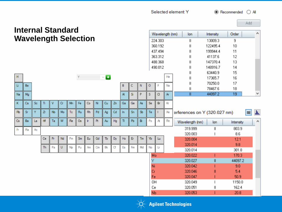
Internal Standard Wavelength Selection
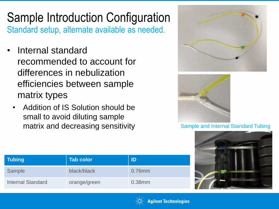
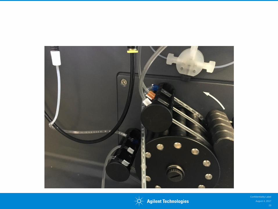
Sample Introduction ConfigurationStandard setup, alternate available as needed.
• Internal standard
recommended to account for
differences in nebulization
efficiencies between sample
matrix types
• Addition of IS Solution should be
small to avoid diluting sample
matrix and decreasing sensitivity Sample and Internal Standard Tubing
Tubing Tab color ID
Sample black/black 0.76mm
Internal Standard orange/green 0.38mm
August 4, 2017
Confidentiality Label
23
Internal Standard Monitoring without Addition
Argon is an effective internal standard when analyzing samples
1. With high concentrations of rare earth and other common
spectral overlapping elements
2. Where sensitivity cannot be jeopardized
- On-line addition is a dilution of all test solutions including the
standards.
- No dilution factor is applied as all test solutions are treated equally
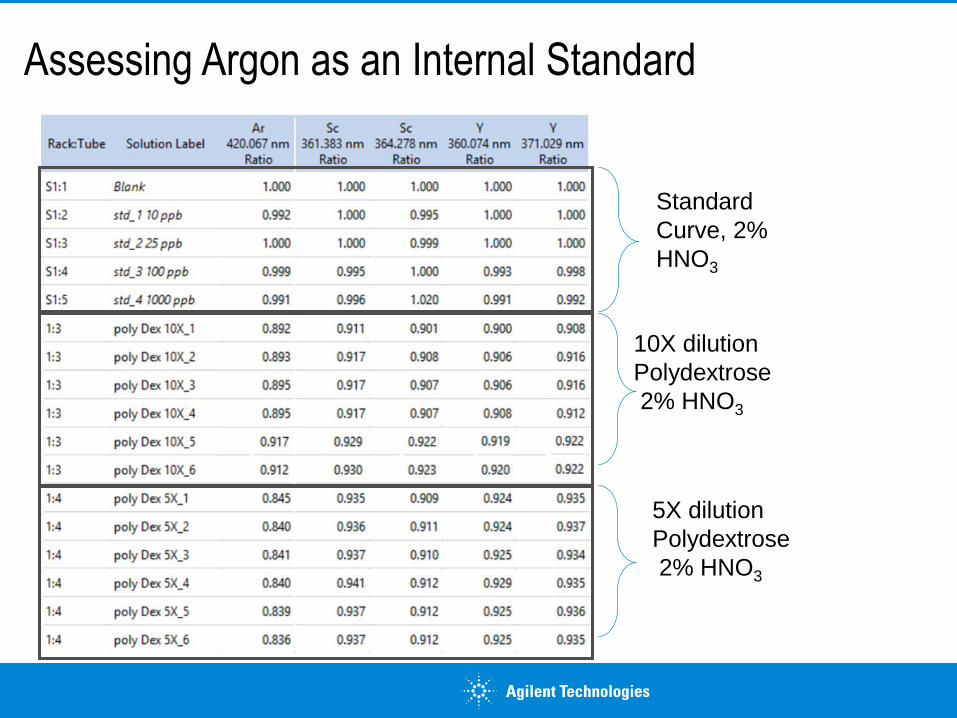
Assessing Argon as an Internal Standard
Standard
Curve, 2%
HNO3
10X dilution
Polydextrose
2% HNO3
5X dilution
Polydextrose
2% HNO3
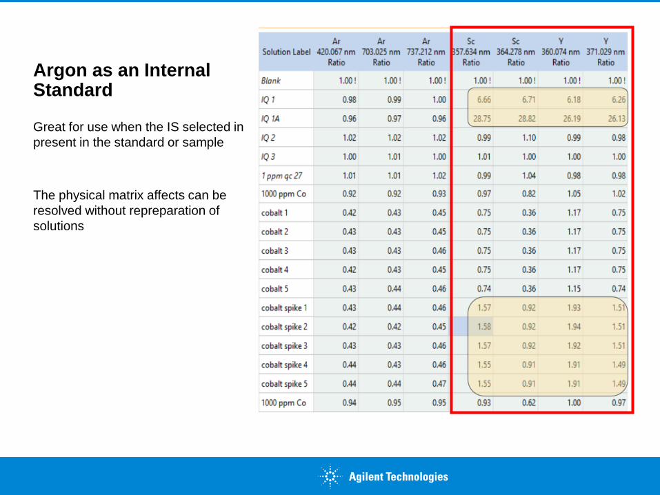
Argon as an Internal Standard
Great for use when the IS selected in
present in the standard or sample
The physical matrix affects can be
resolved without repreparation of
solutions
Interpretation of IS Results (2)
Internal standard ratio for samples
• Close to 1.00
A ratio is calculated referencing the intensity of the internal standard in the samples back to the intensity in first measurement (Blank)
- Ratio = IIS(BLANK) / IIS (SAMPLE)
When ratio is not 1.00, the intensity of the analyte being corrected is adjusted accordingly
- Corrected Concentration Value = C (ANALYTE) x Ratio
• Ratios > 1, the analyte concentration results are adjusted lower
• Ratios < 1, the analyte concentration results are adjusted higher
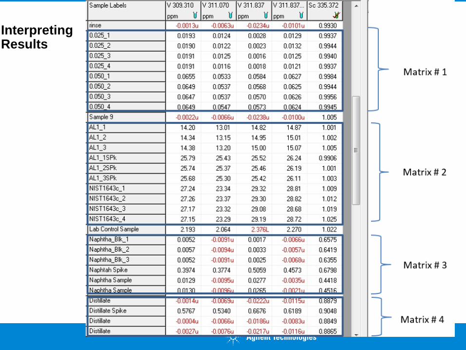
Interpreting Results
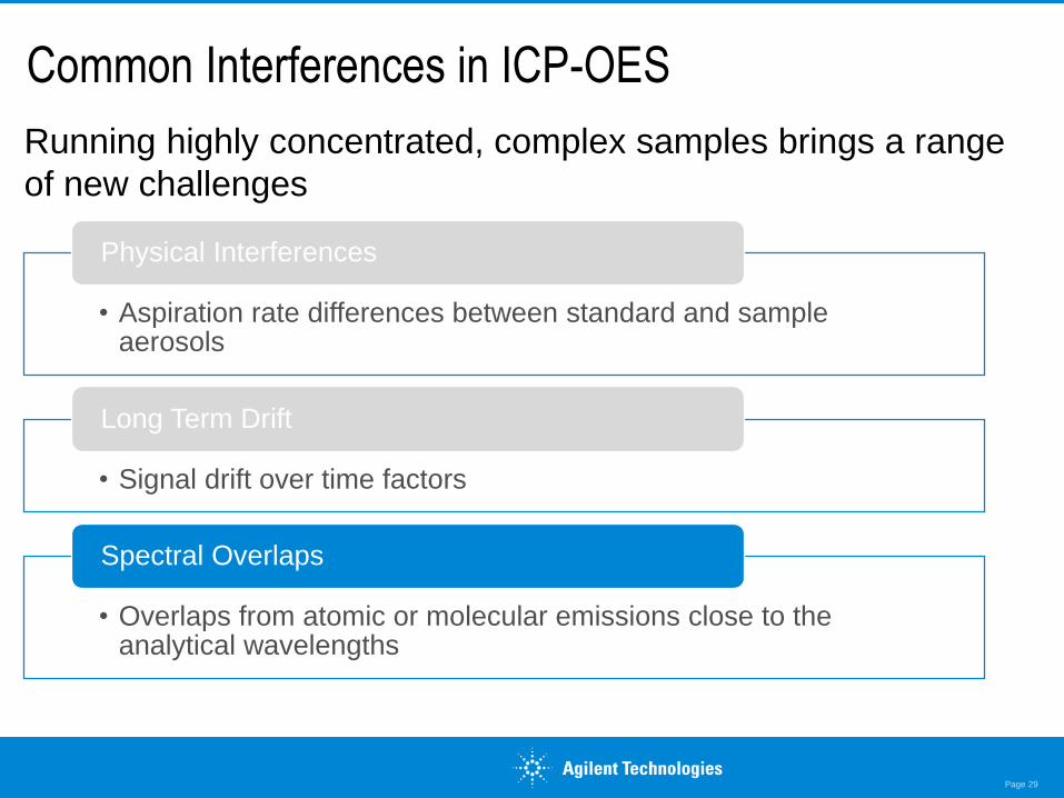
Common Interferences in ICP-OES
Running highly concentrated, complex samples brings a range
of new challenges
Page 29
• Aspiration rate differences between standard and sample aerosols
Physical Interferences
• Signal drift over time factors
Long Term Drift
• Overlaps from atomic or molecular emissions close to the analytical wavelengths
Spectral Overlaps
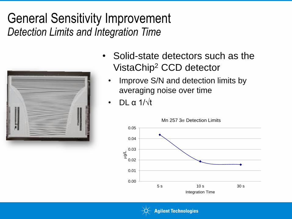
General Sensitivity ImprovementDetection Limits and Integration Time
• Solid-state detectors such as the
VistaChip2 CCD detector
• Improve S/N and detection limits by
averaging noise over time
• DL α 1/√t
0.00
0.01
0.02
0.03
0.04
0.05
5 s 10 s 30 s
mg/L
Integration Time
Mn 257 3s Detection Limits
280
300
320
340
360
380
400
420
440
460
1sec Read time
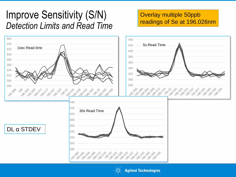
Improve Sensitivity (S/N)Detection Limits and Read Time
280
300
320
340
360
380
400
420
440
5s Read Time
280
300
320
340
360
380
400
420
440
30s Read Time
Overlay multiple 50ppb
readings of Se at 196.026nm
DL α STDEV
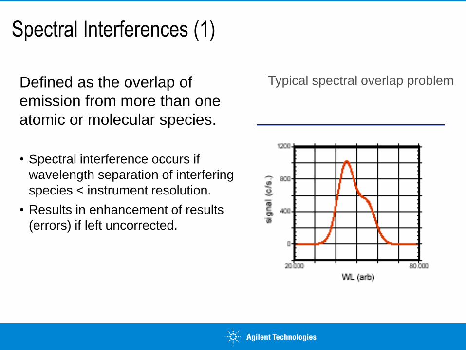
Spectral Interferences (1)
Defined as the overlap of
emission from more than one
atomic or molecular species.
• Spectral interference occurs if
wavelength separation of interfering
species < instrument resolution.
• Results in enhancement of results
(errors) if left uncorrected.
Typical spectral overlap problem
Spectral Interferences (2)
Spectral Interferences arise from
• Other elements present in the samples.
- Major matrix elements
- Elements with large number of intense lines in their spectra.
• Occasionally from plasma or solvent
- Such interferences are typically constant but degrade detection limits.
- Higher background signal and noise
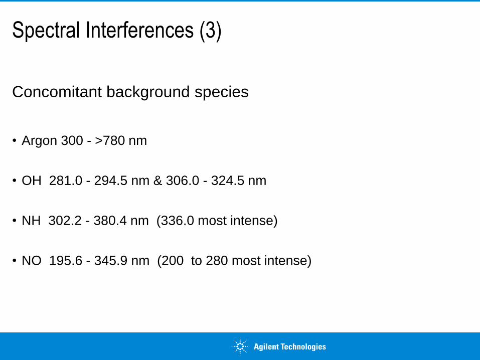
Spectral Interferences (3)
Concomitant background species
• Argon 300 - >780 nm
• OH 281.0 - 294.5 nm & 306.0 - 324.5 nm
• NH 302.2 - 380.4 nm (336.0 most intense)
• NO 195.6 - 345.9 nm (200 to 280 most intense)
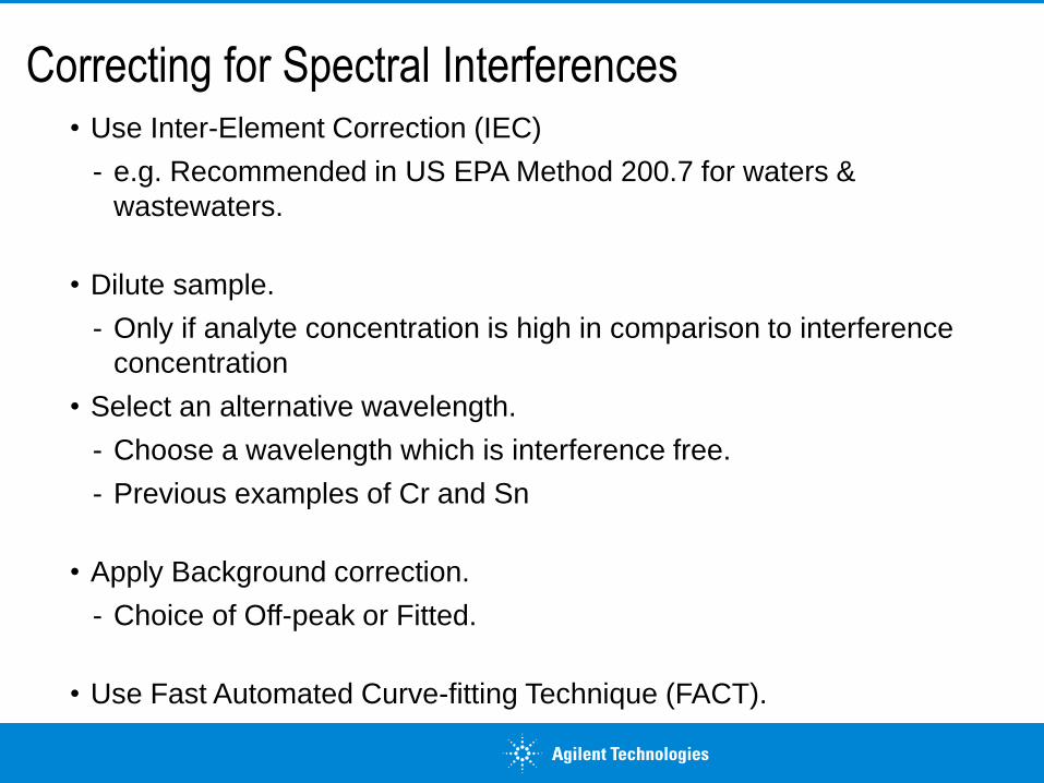
Correcting for Spectral Interferences• Use Inter-Element Correction (IEC)
- e.g. Recommended in US EPA Method 200.7 for waters &
wastewaters.
• Dilute sample.
- Only if analyte concentration is high in comparison to interference
concentration
• Select an alternative wavelength.
- Choose a wavelength which is interference free.
- Previous examples of Cr and Sn
• Apply Background correction.
- Choice of Off-peak or Fitted.
• Use Fast Automated Curve-fitting Technique (FACT).
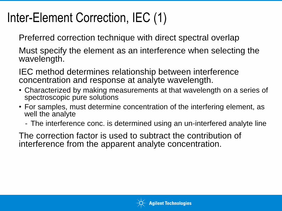
Inter-Element Correction, IEC (1)
Preferred correction technique with direct spectral overlap
Must specify the element as an interference when selecting the wavelength.
IEC method determines relationship between interference concentration and response at analyte wavelength.• Characterized by making measurements at that wavelength on a series of
spectroscopic pure solutions
• For samples, must determine concentration of the interfering element, as well the analyte
- The interference conc. is determined using an un-interfered analyte line
The correction factor is used to subtract the contribution of interference from the apparent analyte concentration.
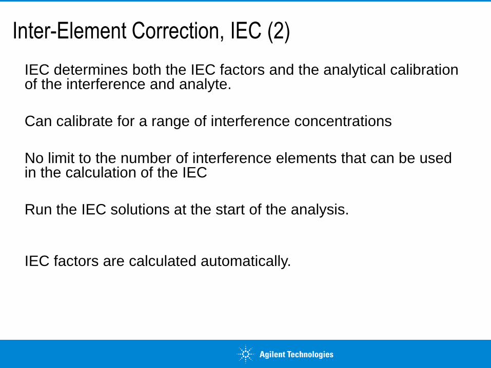
Inter-Element Correction, IEC (2)
IEC determines both the IEC factors and the analytical calibration of the interference and analyte.
Can calibrate for a range of interference concentrations
No limit to the number of interference elements that can be used in the calculation of the IEC
Run the IEC solutions at the start of the analysis.
IEC factors are calculated automatically.
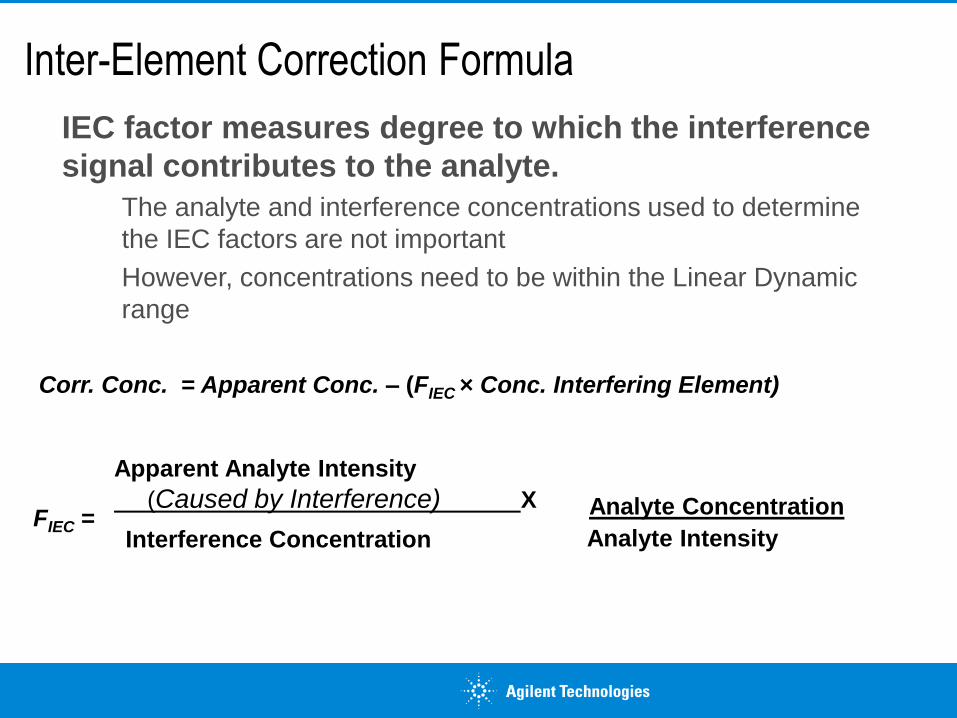
Inter-Element Correction Formula
Corr. Conc. = Apparent Conc. – (FIEC × Conc. Interfering Element)
FIEC =
IEC factor measures degree to which the interference
signal contributes to the analyte.
The analyte and interference concentrations used to determine
the IEC factors are not important
However, concentrations need to be within the Linear Dynamic
range
Apparent Analyte Intensity
(Caused by Interference) X
Interference Concentration
Analyte Concentration
Analyte Intensity
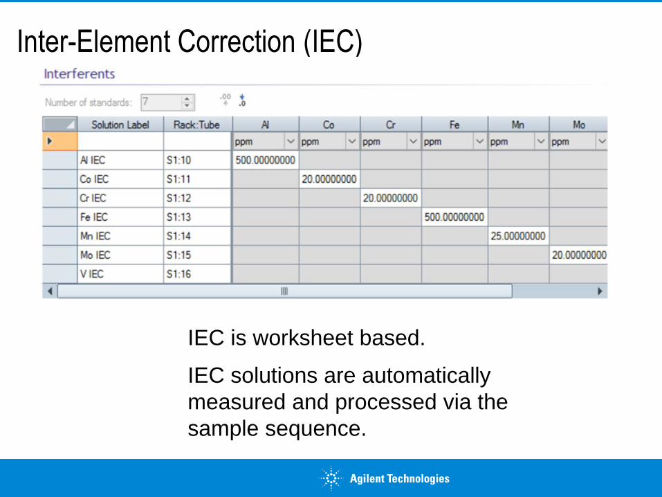
Inter-Element Correction (IEC)
IEC is worksheet based.
IEC solutions are automatically
measured and processed via the
sample sequence.
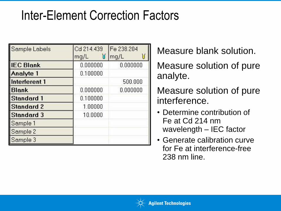
Inter-Element Correction Factors
Measure blank solution.
Measure solution of pure analyte.
Measure solution of pure interference.
• Determine contribution of Fe at Cd 214 nm wavelength – IEC factor
• Generate calibration curve for Fe at interference-free 238 nm line.
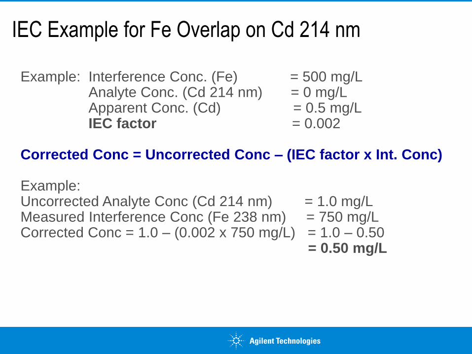
IEC Example for Fe Overlap on Cd 214 nm
Example: Interference Conc. (Fe) = 500 mg/LAnalyte Conc. (Cd 214 nm) = 0 mg/LApparent Conc. (Cd) = 0.5 mg/LIEC factor = 0.002
Corrected Conc = Uncorrected Conc – (IEC factor x Int. Conc)
Example: Uncorrected Analyte Conc (Cd 214 nm) = 1.0 mg/LMeasured Interference Conc (Fe 238 nm) = 750 mg/LCorrected Conc = 1.0 – (0.002 x 750 mg/L) = 1.0 – 0.50
= 0.50 mg/L
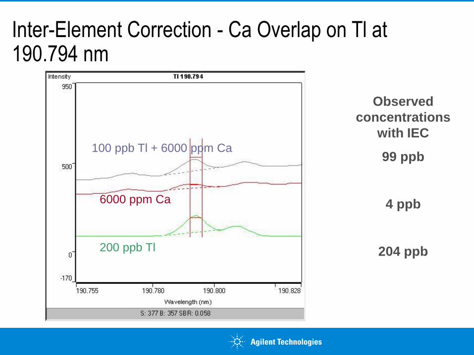
Inter-Element Correction - Ca Overlap on Tl at 190.794 nm
Observed
concentrations
with IEC
99 ppb
4 ppb
204 ppb200 ppb Tl
100 ppb Tl + 6000 ppm Ca
6000 ppm Ca
Disadvantages of IEC
Tedious and time-consuming work to calculate interference factors before actually running program
There could be more than one interference at the line of interest complicating the factors.
If any parameters in program are altered, the correction factors should be re-examined e.g.
- Pump rate, stabilization time, replicate read time, integration time
- ALL plasma parameters.
Factors are calculated based on the known concentration of the interfering elements.
- Best to work within the linear range of both the analyte and interference to avoid bias.
Internal Standard corrections (where used) must be applied BEFORE IEC factors are calculated.

Overcoming Background InterferencesBackground Correction
• Off-peak
- User selects background points.
Modern Corrections
Fitted
- Peak shaped functions will be fitted to the analyte peak.
• Fast Automated Curve-fitting Technique (FACT)
- Provides real-time spectral correction using Gaussian peak
models.
Select an alternate wavelength for measurement.
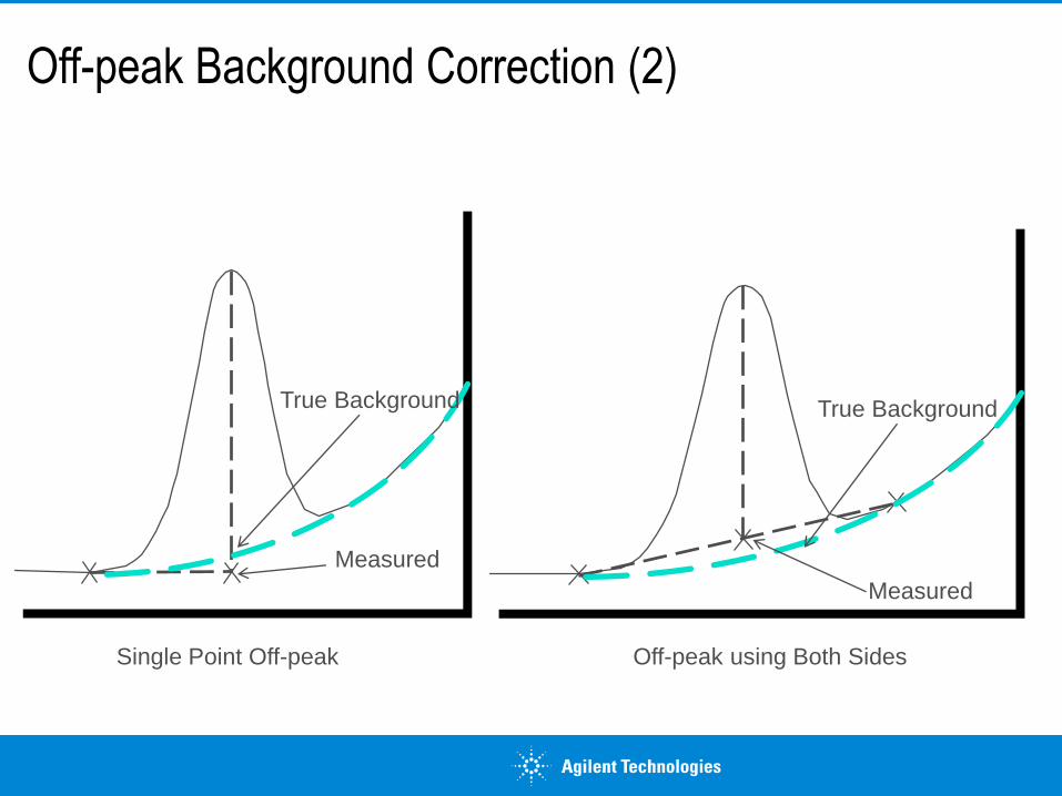
Off-peak Background Correction (2)
True Background
Single Point Off-peak Off-peak using Both Sides
True Background
Measured
Measured
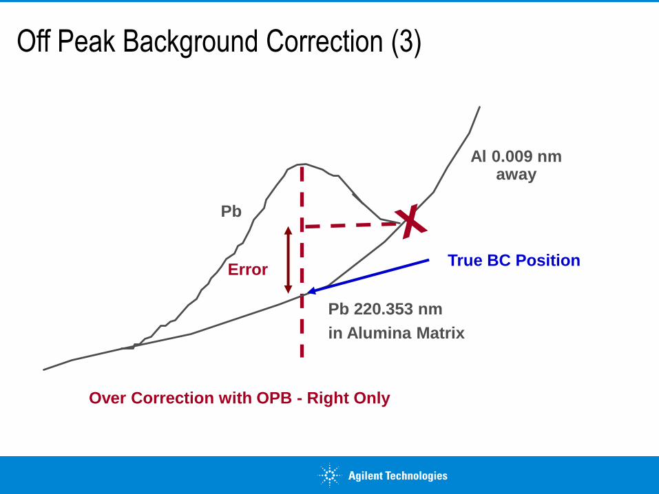
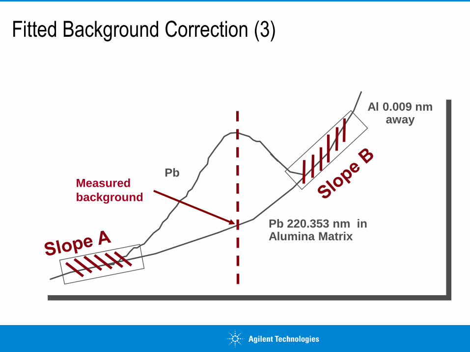
Off Peak Background Correction (3)
Pb 220.353 nm
in Alumina Matrix
Over Correction with OPB - Right Only
Pb
Al 0.009 nm away
True BC PositionError
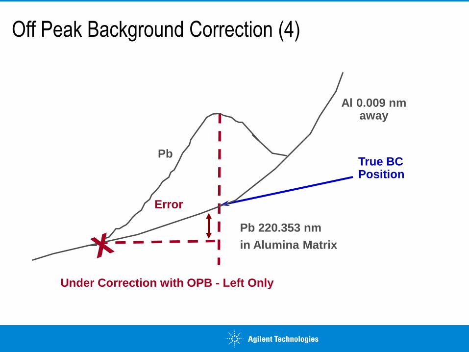
Off Peak Background Correction (4)
Pb 220.353 nm
in Alumina Matrix
Under Correction with OPB - Left Only
Pb
Al 0.009 nm away
True BC Position
Error
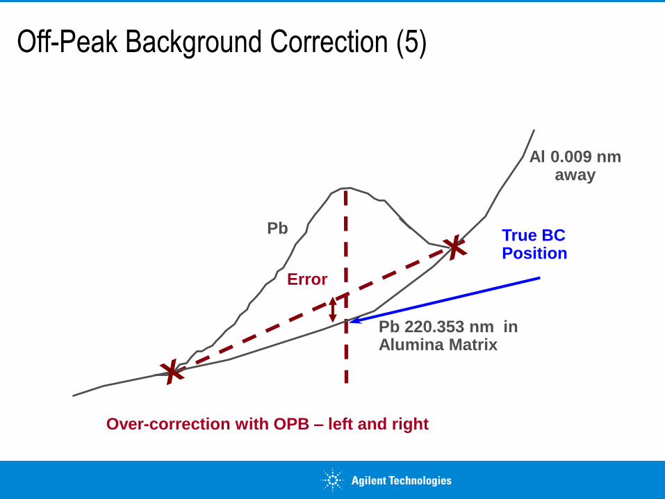
Off-Peak Background Correction (5)
Pb 220.353 nm in Alumina Matrix
Over-correction with OPB – left and right
Pb True BC Position
Al 0.009 nm away
Error
Fitted Background Correction (1)Works by creating a model for the measured spectrum.
Model is composed of:
• An offset component to model unstructured plasma background.
• A slope component to model wings of large distant peaks.
• Three Gaussian peak components to model
- Analyte peak
- Possible interference peak to the left
- Possible interference peak to the right.
• Uses an iterative procedure to estimate the width and positions of peaks.
• Combined with least squares technique to estimate the magnitudes of offset,
slope and peak heights.
• Once model has been fitted, the analyte peak component is removed from the
equation
- Model for background remains.
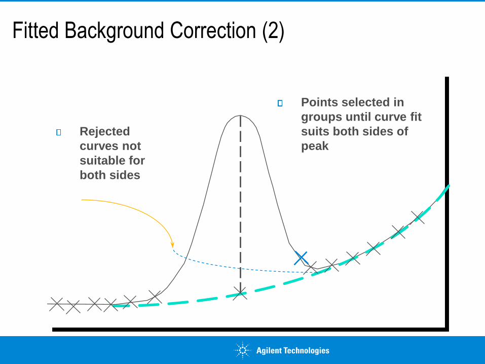
Fitted Background Correction (2)
Points selected in
groups until curve fit
suits both sides of
peak
Rejected
curves not
suitable for
both sides
Pb 220.353 nm in Alumina Matrix
Pb
Al 0.009 nm away
Fitted Background Correction (3)
Measured
background
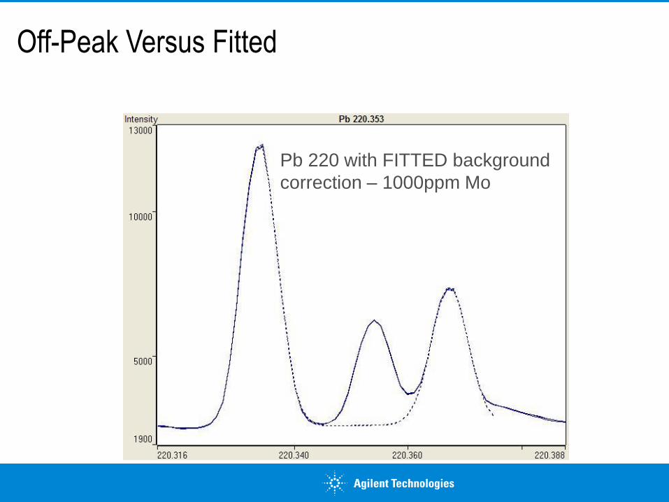
Off-Peak Versus Fitted
Pb 220 with FITTED background
correction – 1000ppm Mo
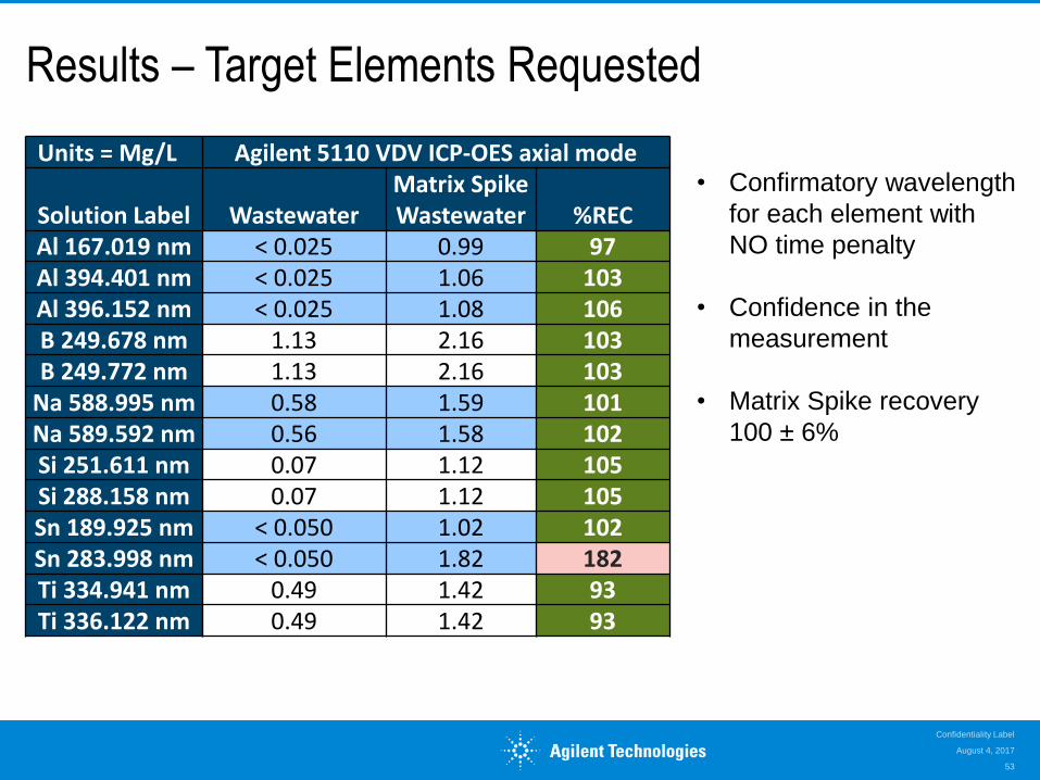
Results – Target Elements Requested
Units = Mg/L Agilent 5110 VDV ICP-OES axial mode
Solution Label WastewaterMatrix Spike Wastewater %REC
Al 167.019 nm < 0.025 0.99 97Al 394.401 nm < 0.025 1.06 103Al 396.152 nm < 0.025 1.08 106B 249.678 nm 1.13 2.16 103B 249.772 nm 1.13 2.16 103
Na 588.995 nm 0.58 1.59 101Na 589.592 nm 0.56 1.58 102Si 251.611 nm 0.07 1.12 105Si 288.158 nm 0.07 1.12 105Sn 189.925 nm < 0.050 1.02 102Sn 283.998 nm < 0.050 1.82 182Ti 334.941 nm 0.49 1.42 93Ti 336.122 nm 0.49 1.42 93
August 4, 2017
Confidentiality Label
53
• Confirmatory wavelength
for each element with
NO time penalty
• Confidence in the
measurement
• Matrix Spike recovery
100 ± 6%
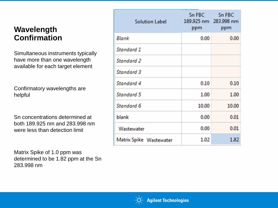
Wavelength Confirmation
Simultaneous instruments typically
have more than one wavelength
available for each target element
Confirmatory wavelengths are
helpful
Sn concentrations determined at
both 189.925 nm and 283.998 nm
were less than detection limit
Matrix Spike of 1.0 ppm was
determined to be 1.82 ppm at the Sn
283.998 nm
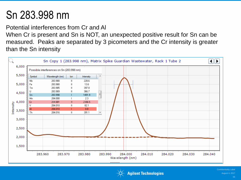
Sn 283.998 nm
August 4, 2017
Confidentiality Label
55
Potential interferences from Cr and Al
When Cr is present and Sn is NOT, an unexpected positive result for Sn can be
measured. Peaks are separated by 3 picometers and the Cr intensity is greater
than the Sn intensity
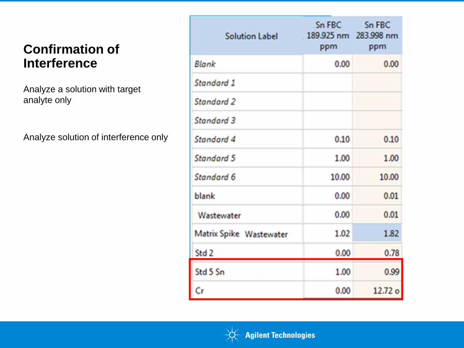
Confirmation of Interference
Analyze a solution with target
analyte only
Analyze solution of interference only
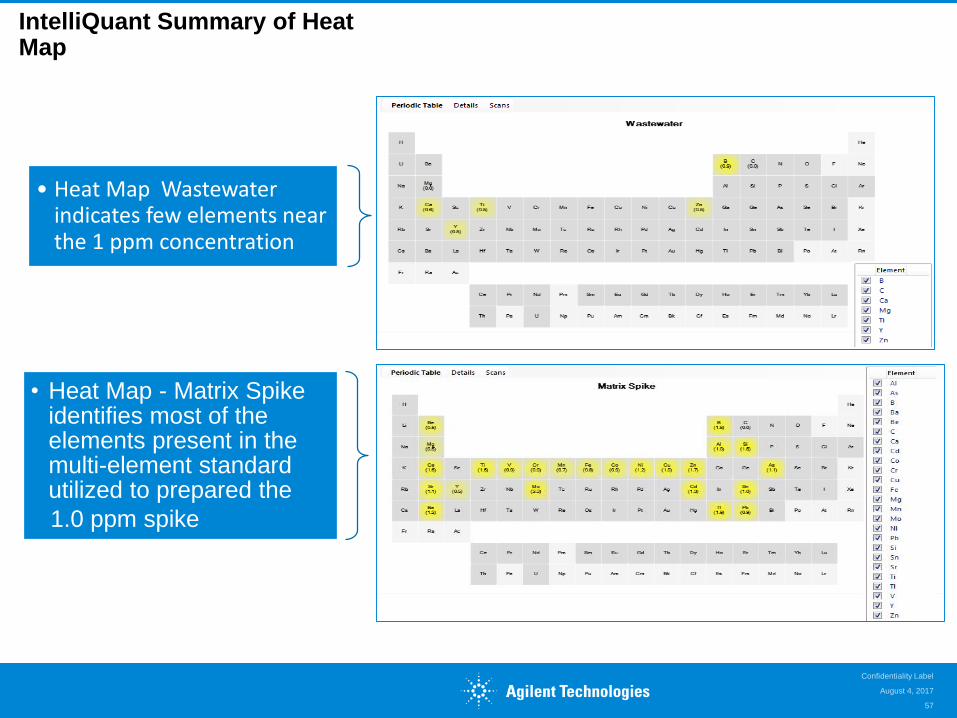
Guardian Wastewater
• Heat Map Wastewater indicates few elements near the 1 ppm concentration
Matrix spike (1 ppm)
• Heat Map - Matrix Spike identifies most of the elements present in the multi-element standard utilized to prepared the
1.0 ppm spike
IntelliQuant Summary of Heat Map
August 4, 2017
Confidentiality Label
57
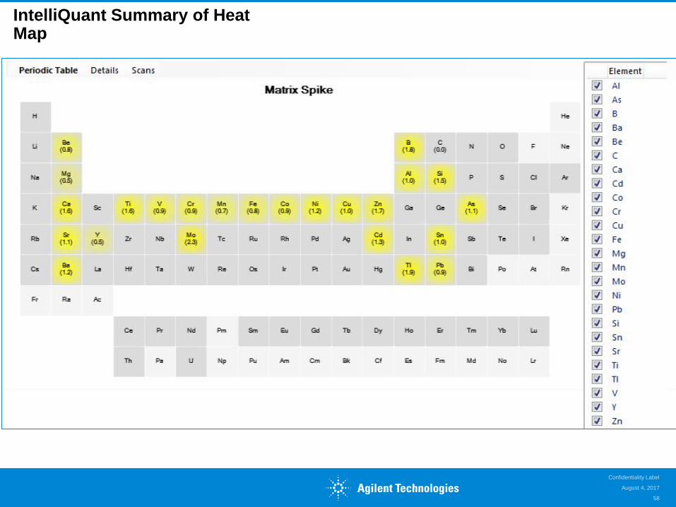
IntelliQuant Summary of Heat Map
August 4, 2017
Confidentiality Label
58
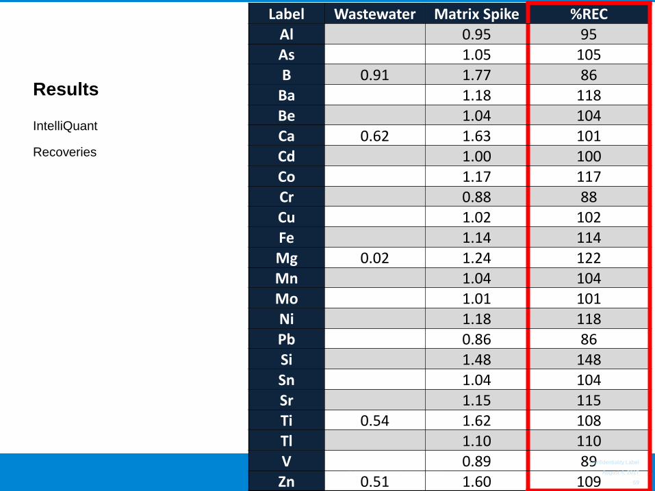
Results
Label Wastewater Matrix Spike %RECAl 0.95 95As 1.05 105B 0.91 1.77 86
Ba 1.18 118Be 1.04 104Ca 0.62 1.63 101Cd 1.00 100Co 1.17 117Cr 0.88 88Cu 1.02 102Fe 1.14 114Mg 0.02 1.24 122Mn 1.04 104Mo 1.01 101Ni 1.18 118Pb 0.86 86Si 1.48 148Sn 1.04 104Sr 1.15 115Ti 0.54 1.62 108Tl 1.10 110V 0.89 89Zn 0.51 1.60 109
IntelliQuant
Recoveries
August 4, 2017
Confidentiality Label
59
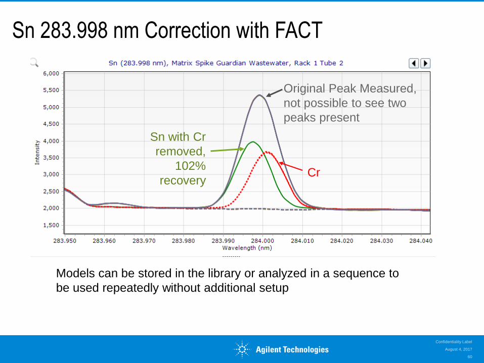
Sn 283.998 nm Correction with FACT
August 4, 2017
Confidentiality Label
60
Cr
Sn with Cr
removed,
102%
recovery
Original Peak Measured,
not possible to see two
peaks present
Models can be stored in the library or analyzed in a sequence to
be used repeatedly without additional setup
Removing Carbon Structures
Deconvolution can also be used to remove molecular, matrix
structures
Low UV wavelengths suffer from these overlaps, however,
there are no alternate wavelengths for use
As = 188.98 nm and 193.7 nm
Se = 196.096 nm
Tl = 190.794 nm, 276.789 nm
Sb = 206.834 nm, 217.582 nm
Pb = 220.353 nm
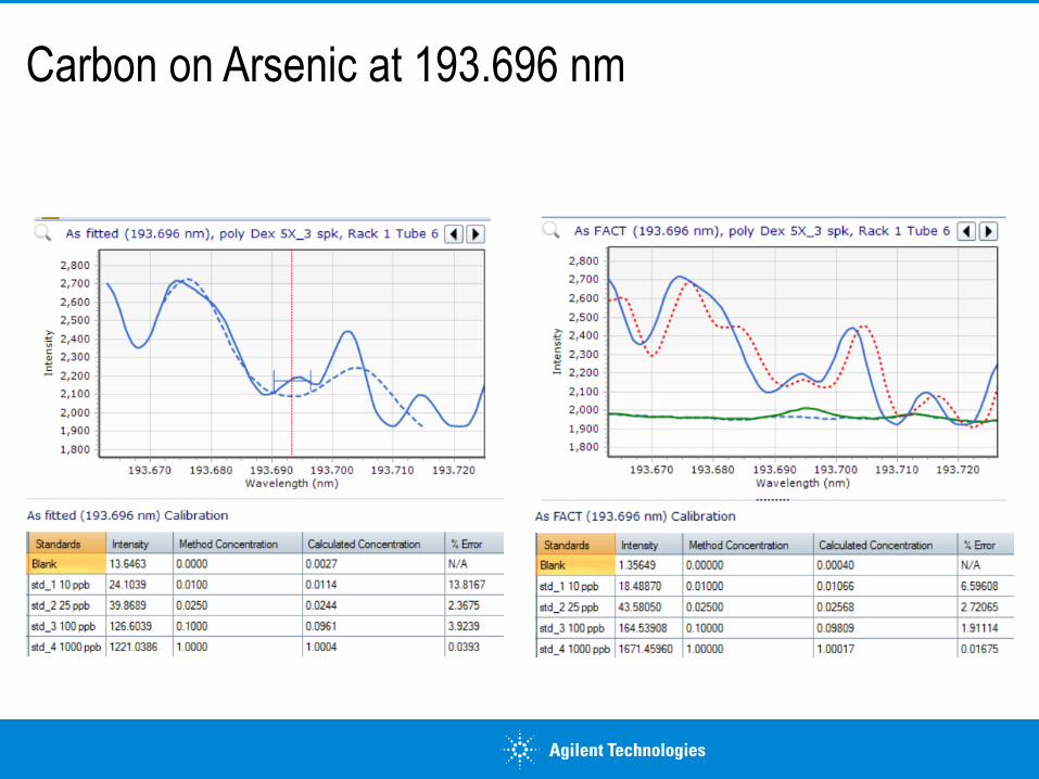
Carbon on Arsenic at 193.696 nm
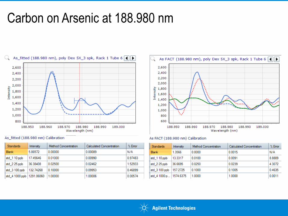
Carbon on Arsenic at 188.980 nm
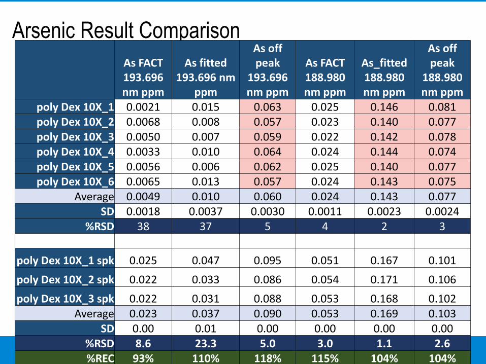
Arsenic Result Comparison
As FACT 193.696 nm ppm
As fitted 193.696 nm
ppm
As off peak
193.696 nm ppm
As FACT 188.980 nm ppm
As_fitted 188.980 nm ppm
As off peak
188.980 nm ppm
poly Dex 10X_1 0.0021 0.015 0.063 0.025 0.146 0.081poly Dex 10X_2 0.0068 0.008 0.057 0.023 0.140 0.077poly Dex 10X_3 0.0050 0.007 0.059 0.022 0.142 0.078poly Dex 10X_4 0.0033 0.010 0.064 0.024 0.144 0.074poly Dex 10X_5 0.0056 0.006 0.062 0.025 0.140 0.077poly Dex 10X_6 0.0065 0.013 0.057 0.024 0.143 0.075
Average 0.0049 0.010 0.060 0.024 0.143 0.077SD 0.0018 0.0037 0.0030 0.0011 0.0023 0.0024
%RSD 38 37 5 4 2 3
poly Dex 10X_1 spk 0.025 0.047 0.095 0.051 0.167 0.101
poly Dex 10X_2 spk 0.022 0.033 0.086 0.054 0.171 0.106
poly Dex 10X_3 spk 0.022 0.031 0.088 0.053 0.168 0.102Average 0.023 0.037 0.090 0.053 0.169 0.103
SD 0.00 0.01 0.00 0.00 0.00 0.00%RSD 8.6 23.3 5.0 3.0 1.1 2.6%REC 93% 110% 118% 115% 104% 104%
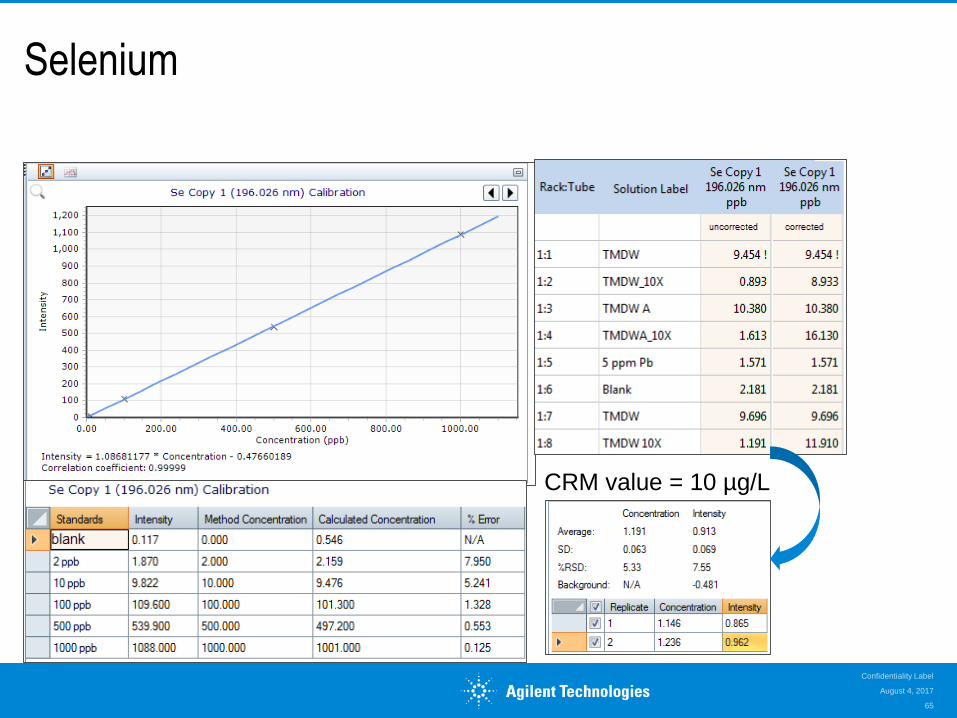
Selenium
August 4, 2017
Confidentiality Label
65
CRM value = 10 µg/L
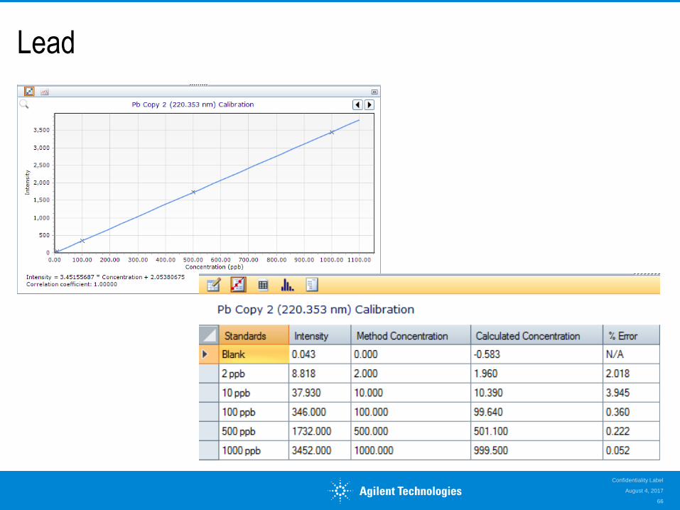
Lead
August 4, 2017
Confidentiality Label
66
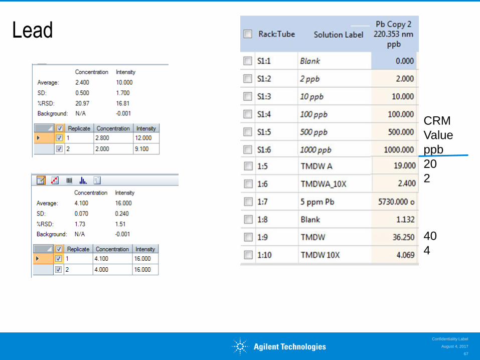
Lead
August 4, 2017
Confidentiality Label
67
CRM
Value
ppb
20
2
40
4
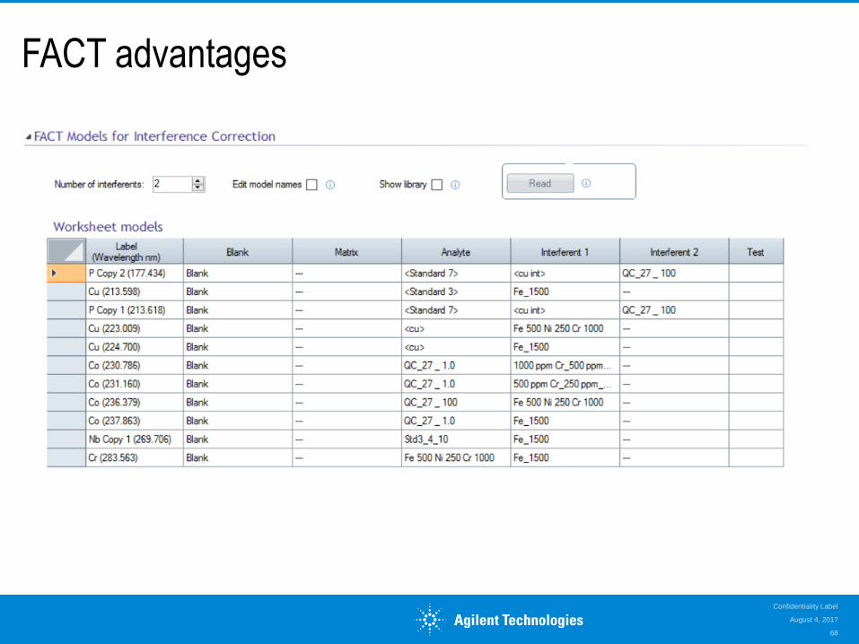
FACT advantages
FACT has a library
Any method can use the models in the library
August 4, 2017
Confidentiality Label
68
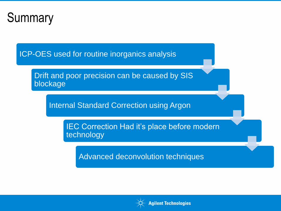
Summary
ICP-OES used for routine inorganics analysis
Drift and poor precision can be caused by SIS blockage
Internal Standard Correction using Argon
Advanced deconvolution techniques
IEC Correction Had it’s place before modern technology

Questions?
70